
Submitted:
13 October 2025
Posted:
14 October 2025
You are already at the latest version
Abstract
The wake characteristics of tidal turbines are significantly influenced by turbulence intensity (TI) and flow velocity in the marine environment. This study employs the Blade Element Momentum (BEM) -CFD method to model two-bladed horizontal tidal turbine wakes, simplifying the turbine geometry while ensuring computational efficiency. The numerical model, validated against experimental data, demonstrates reliable accuracy. Simulations were conducted for background TI levels of 2%, 6%, 10%, 14%, and 18%. Results indicate that wake regions initially expand and then contract, with the contraction point moving closer to the turbine as TI increases. At 2% TI, the wake influence region extends to an axial distance/diameter (X/D) ratio of 20, while at 18% TI, contraction begins at X/D = 4. Low TI results in more extensive low-speed regions, whereas high TI accelerates wake recovery. As TI increases, the wake's turbulence rapidly blends with the background, leading to a reduction in turbulence increments within the wake. Additionally, an analytical wake model for tidal turbines was developed, incorporating turbulence intensity into the formula. The predicted curve exhibited good agreement with the CFD data. This model enables a quick and efficient prediction of wake velocity changes under varying turbulence intensities.
Keywords:
tidal power
; computational fluid dynamics
; wake
; turbines
; blade element model
; experiment
1. Introduction
Tidal energy offers a clean and efficient alternative to fossil fuels due to its reliability, high energy density, predictability, and durability[1]. Over the past two decades, key terms in tidal energy research, such as "tidal turbine" and "wake"[2], highlight the importance of understanding turbine hydrodynamics and wake behavior for optimizing turbine array designs. The wake from upstream turbines influence the inflow conditions of downstream turbines, reducing water kinetic energy and increasing unsteady flow fluctuations[3]. Consequently, the hydrodynamic impact of turbine wakes critically affects the array layout and the overall power performance[4].
Generally, there are two primary methods for exploring the characteristics of turbine wakes: experimentation and numerical modeling. Simmons et al. used experimental methods, and demonstrate that higher flow speeds and turbulence at the turbine tips accelerate wake recovery[3]. Chen conducted wake experiment and found that the wake turbulence was strong and anisotropic[5].
Maganga, Fabrice, and several other researchers have conducted many numerical studies, where the turbine was modeled in its actual shape within the numerical model[6,7,8,9]. Due to the high computational demands of modeling turbines in their real shape, this approach is not suitable for large turbine arrays. As a result, simplified turbine models, such as the porous disk and Blade Element Momentum Theory (BEMT) models, have been proposed. These models approximate the turbine's impact on the flow without detailing the complex geometry of actual blades. This simplification preserves essential wake characteristics while significantly lowering computational costs, making it suitable for wake analysis and array optimization.
Chen and Myers used the porous disk model in laboratory experiments to study wake deficit and shear stress variations, their findings showed that wake velocity rapidly decreases due to momentum loss. In a two-row array, the far wake region (>4D downstream) exhibited a higher velocity deficit compared to a single disk[4,10,11].Batten developed a numerical actuator disk model to investigate the wake characteristics [12]. Shives coupled an actuator disk approach to predict turbine power performance, and the results showed the arrangement of turbine arrays is crucial for effective energy capture[13]. Churchfield modelled tidal turbine using rotating actuator lines to study wake and power performance of different tidal arrays[14].
Ambient turbulence intensity plays a significant role in turbine wake dynamics, influencing the wake's shape, length. Edmunds demonstrated that increased turbulence intensity in the rotor region, particularly near the wake boundary, improves momentum transfer downstream[15]. Gaurier and Mycek revealed that turbine wake recovers faster at higher turbulence [16,17], Nuernberg found that the turbulence intensity in the wake field first increases and then decreases [18]. While high ambient turbulence intensity appears to aid in wake recovery, Mycek’s study showed that the mean power performance of a single turbine is hardly influenced by varying turbulence intensity[17], with the main impact occurring on the inflow of downstream turbine arrays. High turbulence intensity may pose a challenge to the turbine's fatigue and safe. Vinod and Maganga both found that high turbulent intensity caused greater fluctuations in turbine thrust[19,20,21].
To achieve the industrial goals of tidal energy, optimizing the layout of turbine arrays in marine environments is a key objective. Similar to the Jensen model commonly used in wind energy, analytical models for tidal turbines have been developed to predict wake characteristics. These models can be effectively integrated with large-scale marine models such as FVCOM, and can be applied in turbine array optimization of marine sites.
Lam developed an analytical turbine wake model by modifying the Gaussian probability distribution equation, demonstrating strong predictive accuracy for wake velocity [22,23]. In addition to the wake model for horizontal axis turbines, Lam also developed an analytical wake model for vertical axis turbines[24]. Jordan studied different turbine arrays performance using the analytical model FLORIS in ocean model Thetis[25], Brutto developed a wake equation that can be applied in conjunction with Jensen's equation to predict wake velocity[26]. While the wake characteristics and analytical models have been studied by many researchers, the effect of turbulence intensity on wake shape and how to incorporate this influence into the analytical model still requires further investigation.
The aim of this work is to investigate the influence of turbulence intensity on wake dynamics and to develop an analytical wake model that incorporates the effects of turbulence intensity. Section II outlines the theoretical framework of the BEM-CFD numerical model. Section III validates the numerical model by comparing its predictions with experimental data. The numerical results demonstrate strong agreement with the experimental data. In Section IV, we investigate the influence of varying background turbulence intensities, from 2% to 18%, on the wake's expansion and range. Section V proposes an analytical wake model to predict the wake and compares it with CFD data. Finally, summarizes the key conclusions of this study.
2. CFD-BEM Coupled Model
The Blade Element Momentum (BEM) theory is a two-dimensional hydrofoil method widely used in the design of blades for wind and tidal turbines. Viterna and Myers applied BEM theory to the design of wind turbine and tidal turbine, respectively [27,28].
To improve computational efficiency, some researchers have successfully applied the BEM method to simplify tidal turbines in CFD numerical models. This approach simplifies the turbine by dividing the rotating plane into different annular sections, with each section calculated individually.
Guo and Masters both utilized a BEM-CFD numerical model to simplify the horizontal-axis tidal turbine and investigate the wake recovery and other associated characteristics[29,30]. In addition to horizontal-axis turbines, vertical-axis turbines can also be modeled using the BEM-CFD method [31]. Given the extensive research on BEM-CFD modeling of tidal turbine wakes[32,33,34], the theory has been thoroughly introduced in the literatures. This paper provides only a brief overview of the coupled BEM-CFD model.
The coupled BEM-CFD model represents the full turbine rotor geometry using the BEM method in the numerical domain, while the surrounding flow is governed by the Reynolds-averaged Navier–Stokes equations. The numerical simulations were conducted using ANSYS Fluent. The governing equations for momentum and mass conservation are presented below.
Mass conservation:
Momentum conservation:
Here, denotes the density of water, t represents time, is the velocity of the water averaged over time, is the spatial distance, is the mean pressure, is the Reynolds stress, which must be resolved using a turbulence model, is the viscosity, is the component of the gravitational acceleration, and is a source term added to the , y, or z momentum equations. The user-defined function of Fluent was used to define the added source term.
The resultant velocity of the blade element, , is based on BEM theory and a and b are the axial and tangential flow induction factors, respectively. When coupled with CFD, in this equation can be replaced by the local velocity and the tangential flow induction factor b can be calculated from the local velocities and , . The axial and tangential momentum loss terms of the disk region, which represent the turbine in the CFD domain are and , respectively.
Here, c is the length of the blade chord at radius r, r is the radius of the annular ring, e is the disk thickness, which equals 0.1–0.2 of the blade chord length[33], B is the number of blades, φ is the flow angle in the plane of rotation, Cl and Cd are the lift and drag coefficients of the hydrofoil, respectively, and Ft is the blade tip loss factor, which is expressed as:
where R is the turbine diameter.
A flowchart of the coupled model is shown in Figure 1.
2.1. Validation of the Numerical Model
The validation experiment was conducted in the circulating flume at the National Ocean Technology Center, Tianjin, China. A two-blade horizontal axis turbine was positioned at the center of the flume as shown in Figure 2. The dimensions of the flume were 70 m in length, 1.6 m in width, and 2 m in height.
The water depth was maintained at 1.2 m, and the incoming flow was set to 0.489 m/s. The turbine had a diameter of 0.8 m, with a geometric scale of 1:15. The incident flow velocity corresponded to a real-life velocity of 1.9 m/s.
The time-varying velocity components were measured using a NORTEC acoustic doppler velocimeter, which captures velocity data with high temporal resolution. The sampling frequency was set to 200 Hz. Four curves, labeled 01, 02, 03, and 04, are shown in Figure 2, with curve 01 representing the centerline. The adjacent measuring points for each line were spaced 20 cm apart, and the four lines were separated by 10 cm. Further experimental details can be referenced in the study by[35].
The numerical model was validated against experimental results. The domain of the numerical model matched that of the experimental setup, with the incoming velocity set to 0.489 m/s. The computational domain dimensions were 25 m × 1.6 m × 1.2 m. The CFD parameters are detailed in Table 1.
The results from the coupled numerical and experimental models are presented in Figure 3. The dots represent the experimental data, while the line depicts the simulation data. The equation for the deficit coefficient is provided in Eq. (7).
Here, is the free-stream flow velocity and is the wake velocity.
Table 2 presents the mesh independence results, showing the wake deficit at 8D downstream of centerline. Four cases were calculated in total, with δ representing the relative error, Δthe absolute error, and the experimental wake deficit at 8D being 0.20. The results indicate that as the number of mesh nodes increases, the wake deficit approaches the experimental results. The minimum deficit occurs in Case01, with 5.1 × 10⁶ mesh nodes, while the second closest result is Case02, with 6.3 × 10⁵ mesh nodes. For meshes coarser than case02, the error between simulation and experiment becomes relatively large.
Since the deficit between Case01 and Case02 is very small, the focus shifts to computational efficiency. The computational time for Case 02 is under 1 hour, whereas for Case 01, it is nearly 6 hours. Therefore, for both accuracy and efficiency, the mesh with 6.3 × 10⁵ nodes (Case 02) was selected for the subsequent analysis.
The experimental data indicate that the wake deficit decreases as the axial distance increases. The deficit coefficient around the centerline is larger than that behind the turbine tip. Specifically, the deficit of the centerline is 0.4 at 4 X/D (axial distance/diameter of turbine), 0.29 at 6 X/D, and 0.09 at 12 X/D; For curve 04, the deficit is 0.21 at 4 X/D, 0.18 at 6 X/D, and 0.08 at 12 X/D. The error analysis between the simulation data and the experimental data is presented in Table 3, where represents the relative error and represents the absolute error.
As the axial distance increases, both and decrease. The discrepancy between the numerical and experimental results is slightly larger at shorter axial distances. This difference may be attributed to the absence of swirling in the coupled model, which contrasts with the rotating blades of a real turbine. Consequently, the near-wake region exhibits a greater variance. However, as the axial distance increases, the impact of swirling diminishes, leading to improved agreement between the numerical and experimental models. Given that this coupled numerical model is intended primarily for large array studies, this level of agreement is considered acceptable.
2.2. Analysis of the Turbulence Intensity
We calculated five cases with varying background turbulence intensity (TI) values—2%, 6%, 10%, 14%, and 18%—using the numerical model. The background TI was defined in the velocity inlet boundary conditions of ANSYS Fluent. To study the influence region of the wake, the domain of the numerical model was set to 20 m × 4 m × 4 m, with an incident velocity of 2 m/s. All other parameters remained consistent with those of the validated numerical model.
Figure 4 illustrates the velocity contours for X/D ranging from −4 to 20 and Z/D ranging from −4 to 4, for turbulence intensities (TI) of 2% and 18%. In both cases, the wake regions expand. The low-speed area for TI = 2% is larger than that for TI = 18%, indicating that the water flow in the wake with TI = 18% recovers faster than that with TI = 2%. The extent of the contour lines under the same velocity conditions initially expands and then contracts.At X/D = 20, the 2.0 m/s contour line for TI = 2% is still expanding, while the 2.0 m/s contour line for TI = 18% is already contracting. This phenomenon is discussed in detail in the following section.
Figure 5 illustrates the TI contours for boundary conditions set at (a) 2% and (b) 18%. In Figure 5a, TI increases notably as water passes through the tidal turbine, decreasing as axial distance increases.Figure 5b demonstrates that the TI across the entire domain gradually diminishes with increasing axial distance. As water flows through the tidal turbine, TI experiences a significant increase; however, due to the higher background TI, the elevated TI induced by the wake gradually blends with it. The area exhibiting increased TI due to the wake is relatively limited, less distinct compared to the wake effects observed with a background TI of 2%.
The axial results along the centerline for each case were extracted from the numerical model and are depicted in Figure 6. Figure 6a displays the velocity deficit curve, while Figure 6b shows the TI curve. The deficit coefficient decreases with increasing axial distance and turbulence intensity. The velocity deficit curves for TI = 2% and TI = 6% exhibit close proximity. At X/D=2, the deficit ranges from 0.4–0.6, whereas at X/D = 20, it ranges from 0.15–0.02. This indicates that the turbine wake recovers more swiftly with higher TI.
Figure 6b depicts the TI curve along with the axial distance, showing a notable increase as water passes through the turbine, followed by a decrease with axial distance. The values of TI across all cases are quite similar initially, but distinctions become clearer with greater axial distances. Specifically, TI is approximately 27% at X/D = 2, ranging between 13% and 16% at X/D = 8, and between 8%–12% at X/D = 20.
Figure 7 displays the radial velocity results, illustrating how the influence region varies with changes in axial distance and TI. As axial distance increases, the velocity deficit diminishes under consistent TI conditions. The shapes of the radial deficit curves remain similar, with the primary distinction being the peak intensity around Z/D = 0. This peak decreases in magnitude as axial distance increases.
To discuss this phenomenon in detail, Figure 8 illustrates the influence region for each case where the deficit exceeds 0.05, showing variations with different TI and axial distances.
For background TI of 2%, the influence region ranges from -1.18 to 1.18 (Z/D) at X/D=4, expands to -1.20 to 1.20 (Z/D) at X/D=6, further to -1.25 to 1.25 (Z/D) at X/D=10, and reaches -1.28 to 1.28 (Z/D) at X/D=20, continuing to increase with axial distance.
At 6% background TI, the influence region spans from -1.18 to 1.18 (Z/D) at X/D=4, widens to -1.24 to 1.24 (Z/D) at X/D=10 and X/D=14, and narrows to -1.19 to 1.19 (Z/D) at X/D=20, initially increasing and then decreasing beyond X/D=14.
With 10% background TI, the influence region expands from X/D=4 to X/D=6 and contracts for X/D>8. For 18% background TI, the influence region contracts for X/D>4.
These observations highlight how the extent of the influence region varies with both axial distance and background turbulence intensity.
The range of the turbine wake initially expands and then contracts with increasing axial distance. This contraction starts at different locations depending on the TI values. As TI increases, the onset of wake contraction moves closer to the turbine.
Figure 9 presents the radial results of turbulent intensity (TI) for various cases. In Figure 9a, which depicts TI at an axial distance of X/D=4, the TI values at Z/D=0 (the centerline) across all cases are approximately 20%. As the wake region approaches the centerline, the TI values increase, with varying degrees depending on the background TI values. The magnitude of TI increase due to the turbine is more pronounced when the background TI is low.
Figure 9b displays the radial curve of turbulent intensity (TI) at an axial distance of X/D=10. The TI values at Z/D=0 for different cases range between 12% and 15%. At higher background TI values such as 18% or 14%, TI increases only slightly. When the background TI values are 2%, 6%, or 10%, the TI values around the centerline are similar. The heightened TI induced by the turbine gradually blends with the background TI in these cases.
Figure 9c illustrates the radial curve of turbulent intensity (TI) at X/D=20. Significant changes are observed primarily when the background TI is 2% or 6%. When the background TI values are 18%, 14%, or 10%, the TI values remain nearly unchanged. This suggests that the increase in TI caused by the turbine diminishes, and the TI of the wake becomes well mixed with the background TI at this location. As the background TI increases, the rate at which the wake-field TI mixes with the background TI accelerates.
2.2. Analytical Wake Model
Building upon the previous research, we studied the wake distribution formula for tidal stream turbines. Based on Lam’s formula, which is derived from a Gaussian probability distribution[22], we made improvements. The original study only considered specific turbulence intensities of 3%, 5%, 8%, and 15%, and developed separate wake distribution formulas for each turbulence intensity. In this study, we extended Lam’s approach by incorporating the turbulence intensity parameter into the formula. Compared to the original formula, the new formula includes three additional coefficients, namely a, b, and c, allowing the formula to reflect the influence of turbulence intensity in marine environments. The formula is expressed as follows:
Empirical equations incorporating turbulent intensity are proposed to predict the recovery of the minimum velocity as follows:
Considering that the axial distance between consecutive rows of tidal turbine arrays in the ocean is unlikely to be less than 4D, the above formula is applicable for axial distances greater than or equal to 4D.
The efflux velocity is:
The additional coefficient, incorporating turbulent intensity and axial distance, is:
In this study, the turbine’s CT=0.8 and V∞=2m/s,The comparison between the above formula and numerical simulations is shown in Figure 10.
Table 4 presents the comparison of errors between the analytical wake model and CFD data. Data within the radial distance range of -2R to 2R, with a 2D interval, and the axial distance range of 4D to 12D are selected. It can be observed that the R² value ranges from 0.7861 to 0.9944, and the RMSE ranges from 0.0022 to 0.0355. The proposed predictive formula in this study effectively predicts the variation in wake velocity field with different turbulence intensities.
3. Conclusions
This study investigates the influence of ambient turbulence intensity on the wake dynamics of tidal turbines using a coupled Blade Element Momentum and Computational Fluid Dynamics model. The primary objective was to understand how different levels of background TI affect wake shape, recovery, and interaction with the surrounding flow. The numerical model, validated against experimental data, demonstrates good agreement, thereby confirming its reliability.
1. Wake Influence Region and Turbulence Intensity: The wake influence region initially expands and then contracts as the background TI increases. The point at which contraction begins moves closer to the turbine with higher TI values. As background TI increases, the turbulent intensity within the wake merges more quickly with the surrounding flow, leading to a less pronounced increase in TI within the wake region and indicating faster homogenization with the background TI.
2. Wake Recovery and Velocity Deficit: Higher background TI significantly accelerates the wake recovery process, reducing the extent of low-speed areas. The velocity deficit decreases with increasing axial distance from the turbine, with the deficit around the centerline being higher compared to areas behind the turbine tip. This highlights the non-uniformity of wake recovery and emphasizes the role of background TI in wake dynamics.
3. Implications for Turbine Array Layouts: This study highlights the critical role of considering ambient turbulence intensity (TI) in the design and optimization of tidal turbine arrays. The proposed formula, which reflects the influence of varying turbulence intensities, can be conveniently applied to the study of wake interactions in turbine arrays. Higher TI affects wake dynamics, potentially influencing the overall efficiency and performance of the arrays. However, the impact of high turbulence intensity on the structural integrity of the turbines was not addressed in this study and warrants further investigation.
In summary, besides demonstrating that higher turbulence intensity enhances wake recovery, our study also reveals notable variations in the wake field structure under different turbulence intensities. As turbulence intensity increases, the expansion trend and the affected region of the wake become more pronounced. Beyond the widely studied wake velocity variations, we also investigated the overall turbulence intensity changes within the wake field. Furthermore, we propose a practical analytical wake model that can rapidly predict the wake velocity, providing a useful tool for future studies and applications. This paper provides new insights and tools for optimizing turbine array configurations and elucidating wake evolution mechanisms.
Author Contributions
Conceptualization, E.H. and H.W.; methodology, E.H.; software, E.H.; validation, E.H. and L.Z.; formal analysis, Y.L.; H.W. J.D. Y.W.; writing—original draft preparation, E.H.; writing—review and editing, Y.L. J.D. All authors have read and agreed to the published version of the manuscript.
Funding
This research was funded by the National Natural Science Foundation of China, grant number 42276228.
Acknowledgments
The authors declare no acknowledgements.
Conflicts of Interest
The authors declare no conflict of interest.
References
- Chowdhury, M.S.; Rahman, K.S.; Selvanathan, V.; Nuthammachot, N.; Suklueng, M.; Mostafaeipour, A.; Habib, A.; Akhtaruzzaman, M.; Amin, N.; Techato, K. Current trends and prospects of tidal energy technology. Environment, Development and Sustainability 2020, 23, 8179-8194. [CrossRef]
- Khojasteh, D.; Shamsipour, A.; Huang, L.; Tavakoli, S.; Haghani, M.; Flocard, F.; Farzadkhoo, M.; Iglesias, G.; Hemer, M.; Lewis, M.; et al. A large-scale review of wave and tidal energy research over the last 20 years. Ocean Engineering 2023, 282. [CrossRef]
- Simmons, S.M.; McLelland, S.J.; Parsons, D.R.; Jordan, L.-B.; Murphy, B.J.; Murdoch, L. An investigation of the wake recovery of two model horizontal-axis tidal stream turbines measured in a laboratory flume with Particle Image Velocimetry. Journal of Hydro-environment Research 2018, 19, 179-188. [CrossRef]
- Chen, Y.; Sun, J.; Lin, B.; Lin, J.; Guo, J. Spatial evolution and kinetic energy restoration in the wake zone behind a tidal turbine: An experimental study. Ocean Engineering 2021, 228. [CrossRef]
- Chen, Y.; Lin, B.; Lin, J.; Wang, S. Experimental study of wake structure behind a horizontal axis tidal stream turbine. Applied Energy 2017, 196, 82-96. [CrossRef]
- Maganga, F.; Pinon, G.; Germain, G.; Rivoalen, E. Wake properties characterisation of marine current turbines. In Proceedings of the 3rd International Conference on Ocean Energy, Bilbao, 2010.
- Fabrice, M.; Gr´egory, P.; Gr´egory, G.; Elie, R. Numerical characterisation of the wake generated by marine current turbines farm. icoe 2008.
- Jo, C.-H.; Lee, J.-H.; Rho, Y.-H.; Lee, K.-H. Performance analysis of a HAT tidal current turbine and wake flow characteristics. Renewable Energy 2014, 65, 175-182. [CrossRef]
- Liu, J.; Lin, H.; Purimitla, S.R. Wake field studies of tidal current turbines with different numerical methods. Ocean Engineering 2016, 117, 383-397. [CrossRef]
- Myers, L.E.; Bahaj, A.S. An experimental investigation simulating flow effects in first generation marine current energy converter arrays. Renewable Energy 2012, 37, 28-36. [CrossRef]
- Myers, L.E.; Bahaj, A.S. Experimental analysis of the flow field around horizontal axis tidal turbines by use of scale mesh disk rotor simulators. Ocean Engineering 2010, 37, 218-227. [CrossRef]
- Batten, W.M.; Harrison, M.E.; Bahaj, A.S. Accuracy of the actuator disc-RANS approach for predicting the performance and wake of tidal turbines. Philos Trans A Math Phys Eng Sci 2013, 371, 20120293. [CrossRef]
- Shives, M.; Crawford, C. Tuned actuator disk approach for predicting tidal turbine performance with wake interaction. International Journal of Marine Energy 2017, 17, 1-20. [CrossRef]
- Churchfield, M.J.; Li, Y.; Moriarty, P.J. A large-eddy simulation study of wake propagation and power production in an array of tidal-current turbines. Philos Trans A Math Phys Eng Sci 2013, 371, 20120421. [CrossRef]
- Edmunds, M.; Williams, A.J.; Masters, I.; Croft, T.N. An enhanced disk averaged CFD model for the simulation of horizontal axis tidal turbines. Renewable Energy 2017, 101, 67-81. [CrossRef]
- Gaurier, B.; Carlier, C.; Germain, G.; Pinon, G.; Rivoalen, E. Three tidal turbines in interaction: An experimental study of turbulence intensity effects on wakes and turbine performance. Renewable Energy 2020, 148, 1150-1164. [CrossRef]
- Mycek, P.; Gaurier, B.; Germain, G.; Pinon, G.; Rivoalen, E. Experimental study of the turbulence intensity effects on marine current turbines behaviour. Part I One single turbine. Renewable Energy 2014, 66, 729-746. [CrossRef]
- Nuernberg, M.; Tao, L. Three dimensional tidal turbine array simulations using OpenFOAM with dynamic mesh. Ocean Engineering 2018, 147, 629-646. [CrossRef]
- Maganga, F.; Germain, G.; King, J.; Pinon, G.; Rivoalen, E. Experimental study to determine flow characteristic effects on marine current turbine behaviour. In Proceedings of the 8th European Wave and Tidal Energy Conference, Uppsala, Sweden, 2009.
- Vinod, A.; Han, C.; Banerjee, A. Tidal turbine performance and near-wake characteristics in a sheared turbulent inflow. Renewable Energy 2021, 175, 840-852. [CrossRef]
- Vinod, A.; Banerjee, A. Performance and near-wake characterization of a tidal current turbine in elevated levels of free stream turbulence. Applied Energy 2019, 254, 1-17. [CrossRef]
- Lam, W.-H.; Chen, L.; Hashim, R. Analytical wake model of tidal current turbine. Energy 2015, 79, 512-521. [CrossRef]
- Lam, W.-H.; Chen, L. Equations used to predict the velocity distribution within a wake from a horizontal-axis tidal-current turbine. Ocean Engineering 2014, 79, 35-42. [CrossRef]
- Ma, Y.; Lam, W.H.; Cui, Y.; Zhang, T.; Jiang, J.; Sun, C.; Guo, J.; Wang, S.; Lam, S.S.; Hamill, G. Theoretical vertical-axis tidal-current-turbine wake model using axial momentum theory with CFD corrections. Applied Ocean Research 2018, 79, 113-122. [CrossRef]
- Jordan, C.; Dundovic, D.; Fragkou, A.K.; Deskos, G.; Coles, D.S.; Piggott, M.D.; Angeloudis, A. Combining shallow-water and analytical wake models for tidal array micro-siting. Journal of Ocean Engineering and Marine Energy 2022, 8, 193-215. [CrossRef]
- Brutto, O.A.L.; Nguyen, V.T.; Guillou, S.S.; Thiébot, J.; Gualous, H. Tidal farm analysis using an analytical model for the flow velocity prediction in the wake of a tidal turbine with small diameter to depth ratio. Renewable Energy 2016, 99, 347-359. [CrossRef]
- Viterna, L.A, Corrigan, R.D. Fixed pitch rotor performance of large horizontal axis wind turbines. In Large Horizontal-Axis Wind Turbines (NASA-CP-2230) 1982, 69-85.
- Myers, L.; Bahaj, A.S. Power output performance characteristics of a horizontal axis marine current turbine. Renewable Energy 2006, 31, 197-208. [CrossRef]
- Guo, Q.; Zhou, L.J.; Wang, Z.W. Comparison of BEM-CFD and full rotor geometry simulations for the performance and flow field of a marine current turbine. Renewable Energy 2015, 75, 640-648. [CrossRef]
- Masters, I.; Malki, R.; Williams, A.J.; Croft, T.N. The influence of flow acceleration on tidal stream turbine wake dynamics: A numerical study using a coupled BEM–CFD model. Applied Mathematical Modelling 2013, 37, 7905-7918. [CrossRef]
- Pucci, M.; Spina, R.; Zanforlin, S. Vertical-Axis Tidal Turbines: Model Development and Farm Layout Design. Energies 2024, 17. [CrossRef]
- Turnock, S.R.; Phillips, A.B.; Banks, J.; Nicholls-Lee, R. Modelling tidal current turbine wakes using a coupled RANS-BEMT approach as a tool for analysing power capture of arrays of turbines. Ocean Engineering 2011, 38, 1300-1307. [CrossRef]
- Bai, G.H.; Li, J.; Fan, P.F.; Li, G.J. Numerical investigations of the effects of different arrays on power extractions of horizontal axis tidal current turbines. Renewable Energy 2013, 53, 180-186. [CrossRef]
- M. E. Harrison, W.M.J.B., A. S. Bahaj. A Blade Element Actuator Disc Approach Applied to Tidal Stream Turbines. In Proceedings of the OCEANS 2010. IEEE, 2010, 2010.
- Hou, E.; Du, M.; Jiang, B.; Han, L.; Wu, G.; Wang, X. Study on characteristics of turbine wake and the effect of array arrangement. Proceedings of the Institution of Civil Engineers - Maritime Engineering 2021, 174, 112-123. [CrossRef]
Figure 1.
Flowchart of the blade element momentum (BEM) coupled model.
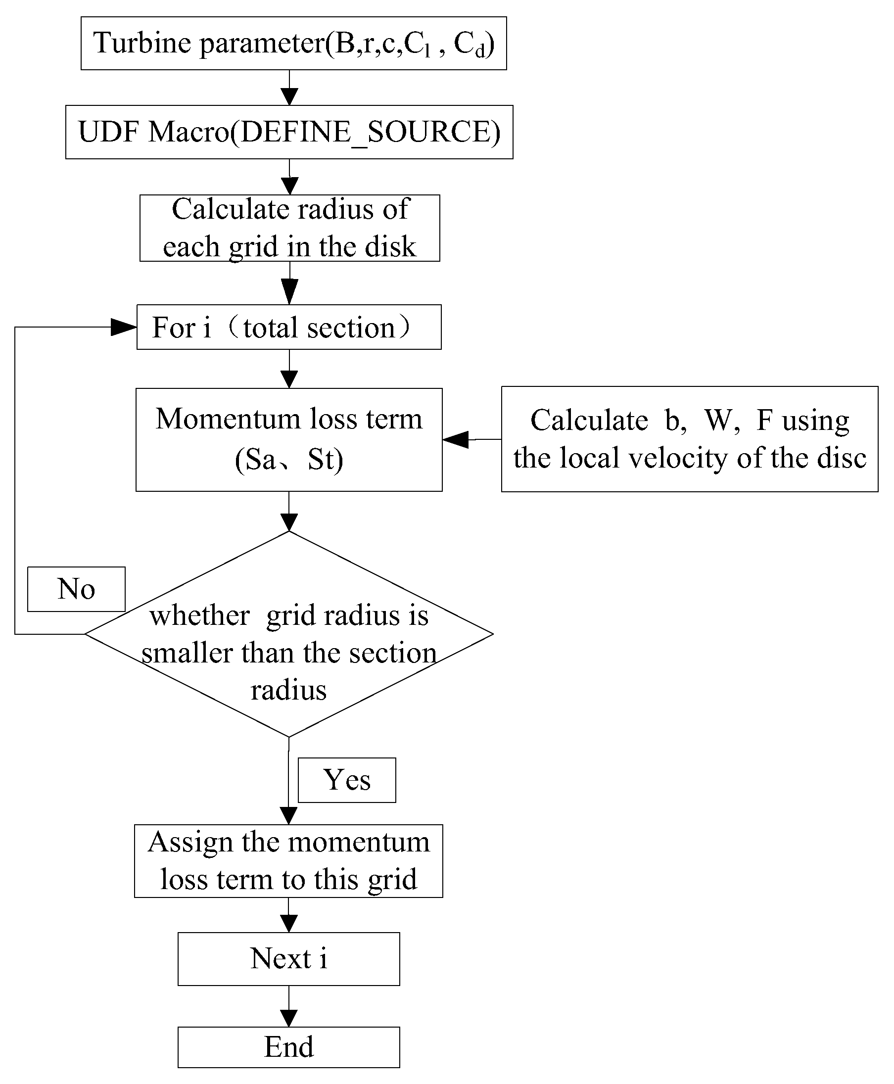
Figure 2.
Experimental turbine and measurement positions.
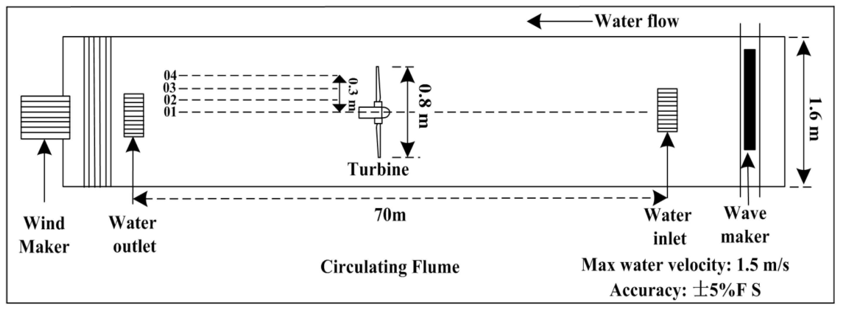
Figure 3.
Simulation and experimental results.
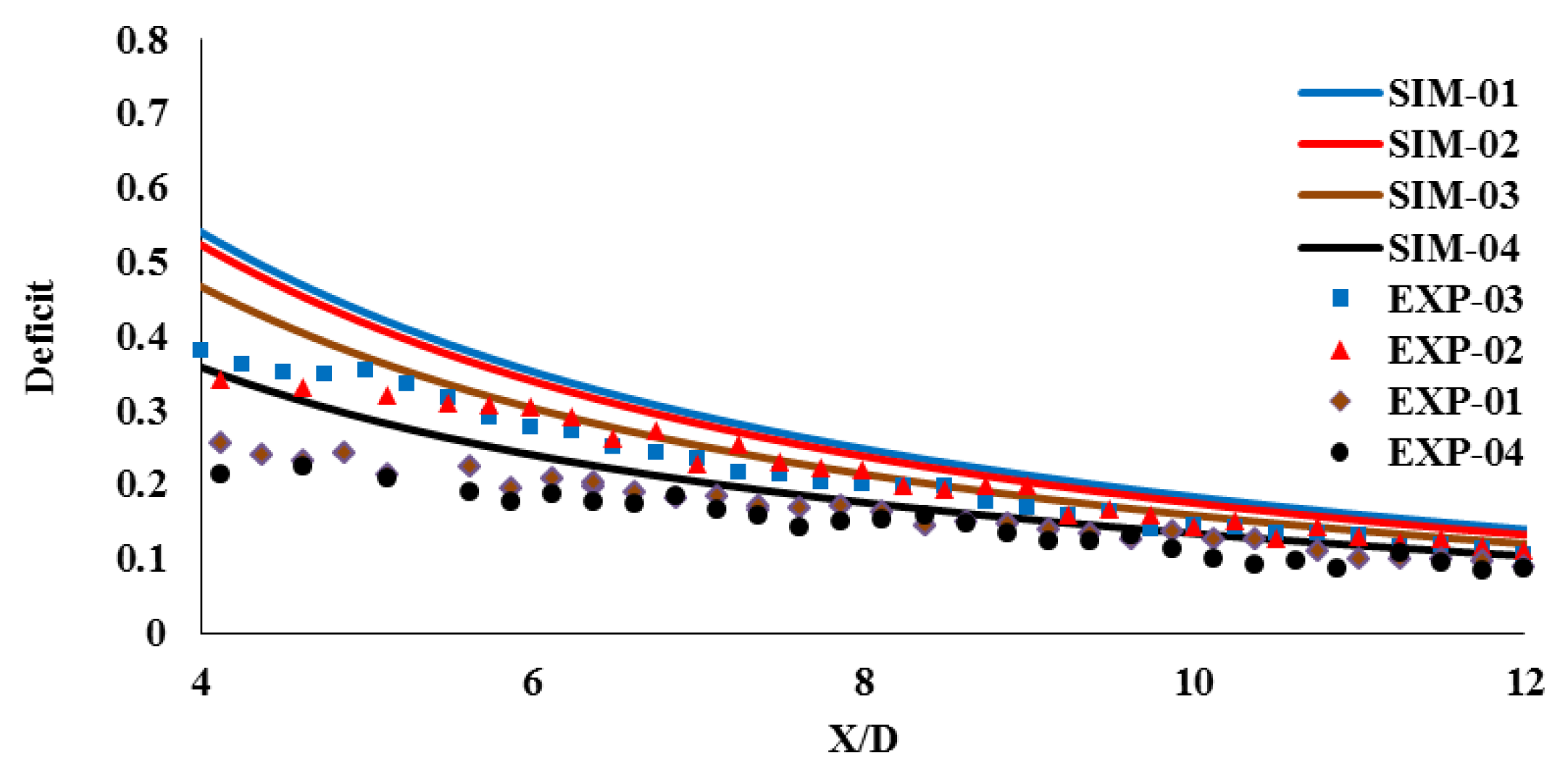
Figure 4.
Velocity contours for background turbulence intensity (TI) values of (a) 2% and (b) 18%.
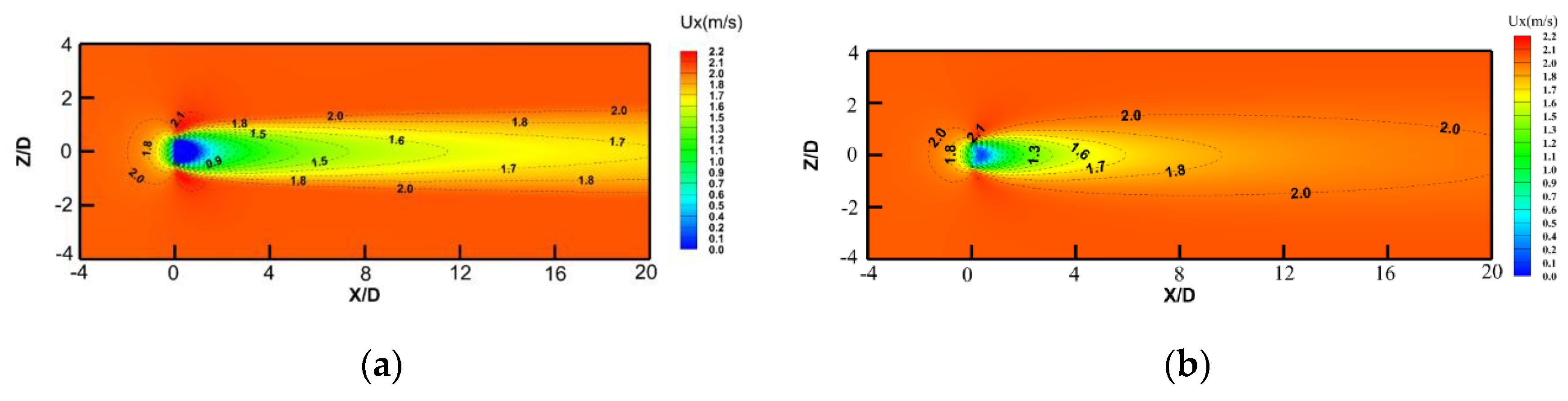
Figure 5.
TI contours for inlet background TI values of (a) 2% and (b) 18%.
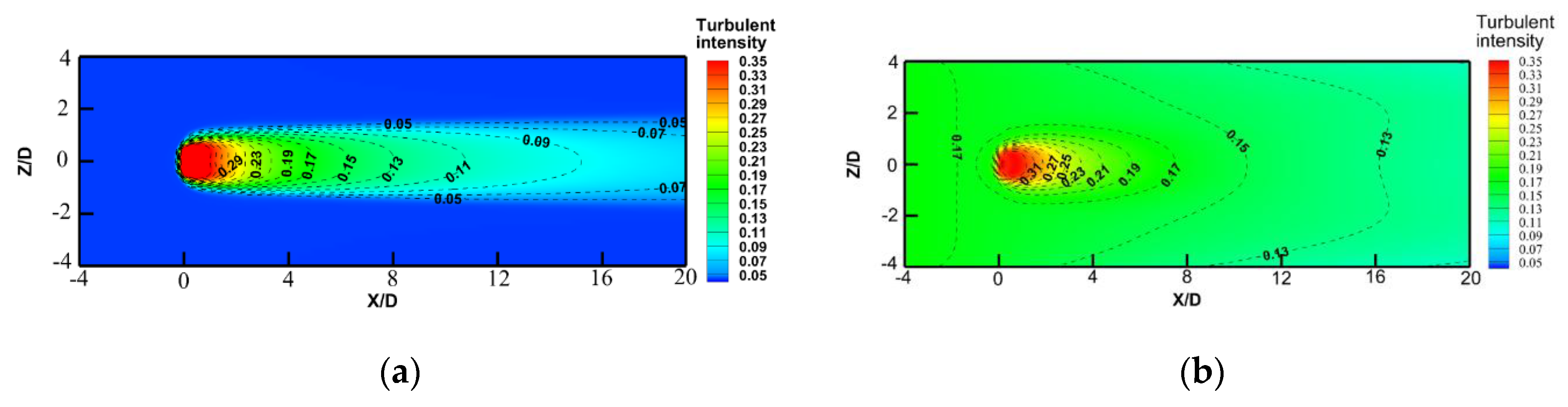
Figure 6.
Axial results for the centerline: (a) the velocity deficit and (b) the TI.
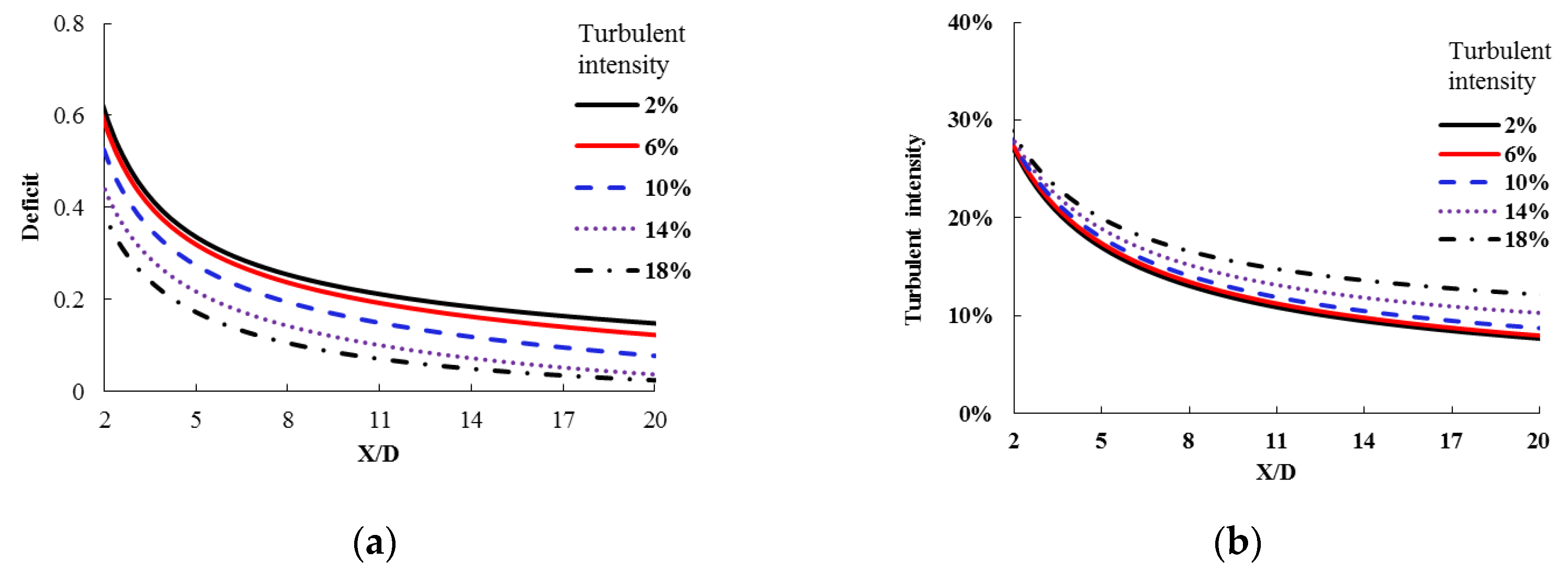
Figure 7.
Radial velocity deficit results: (a) X/D = 4, (b) X/D = 10, and (c) X/D = 20.
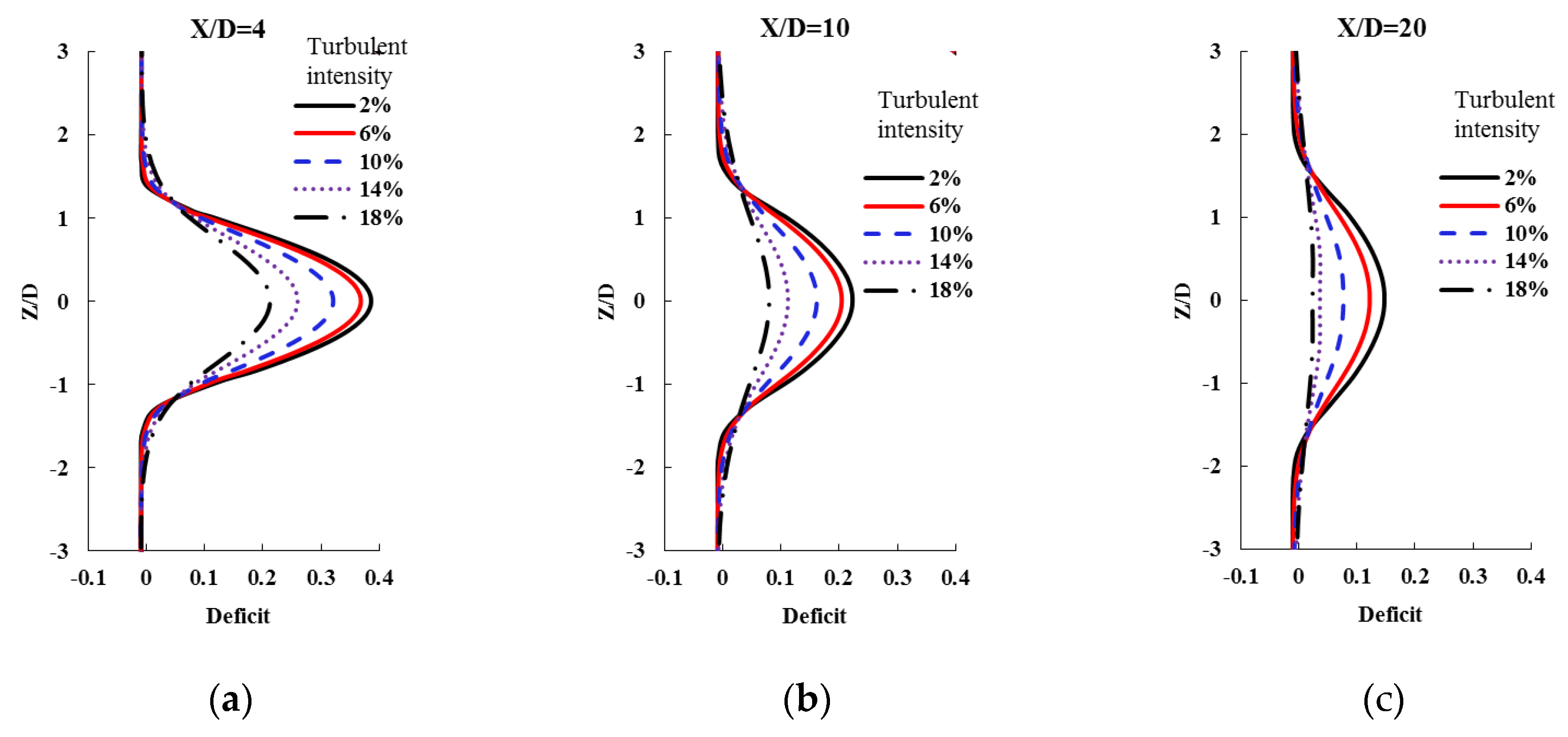
Figure 8.
Influence region (deficit > 0.05).
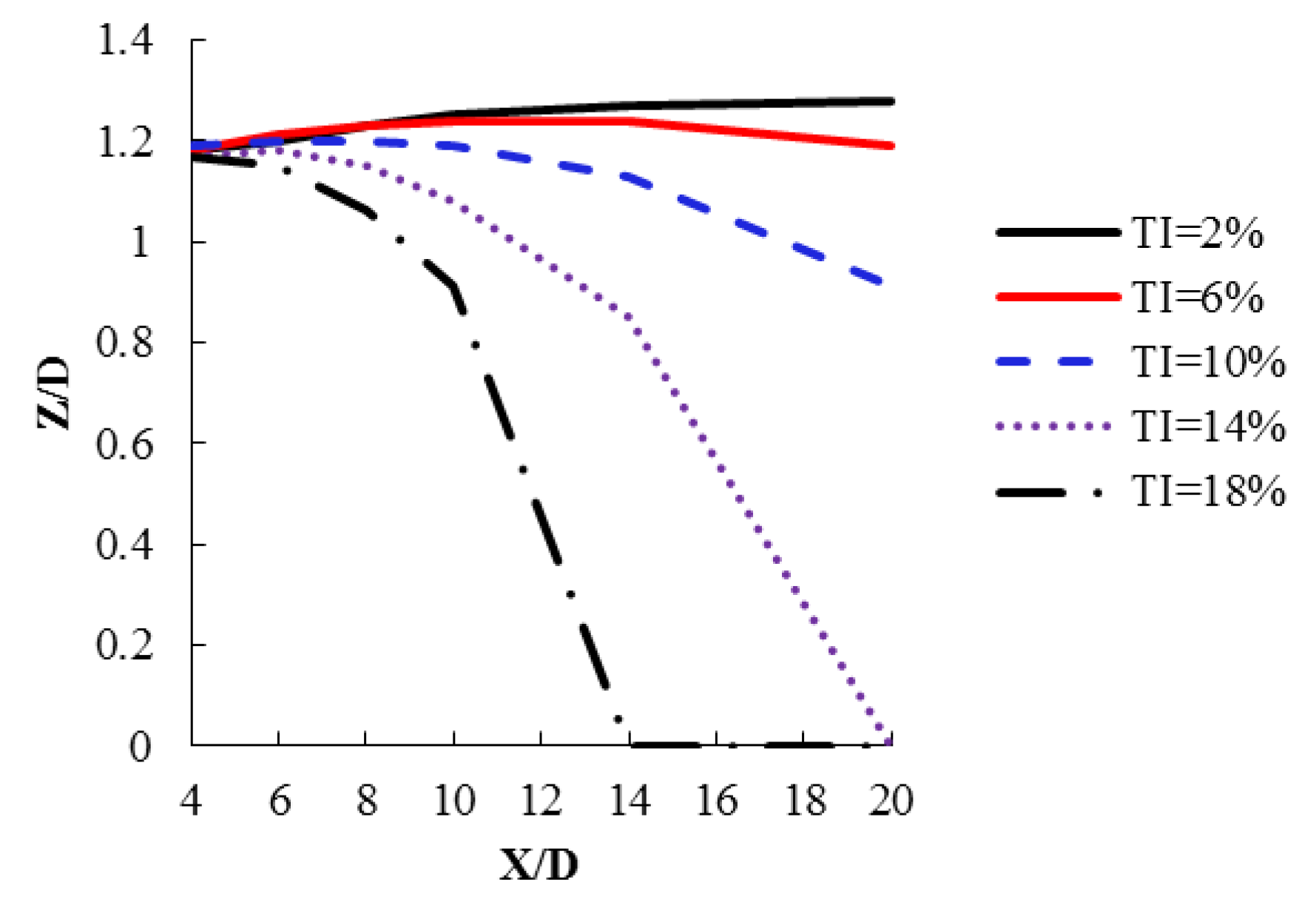
Figure 9.
Radial turbulent intensity results for (a) X/D = 4, (b) X/D = 10, and (c) X/D = 20.
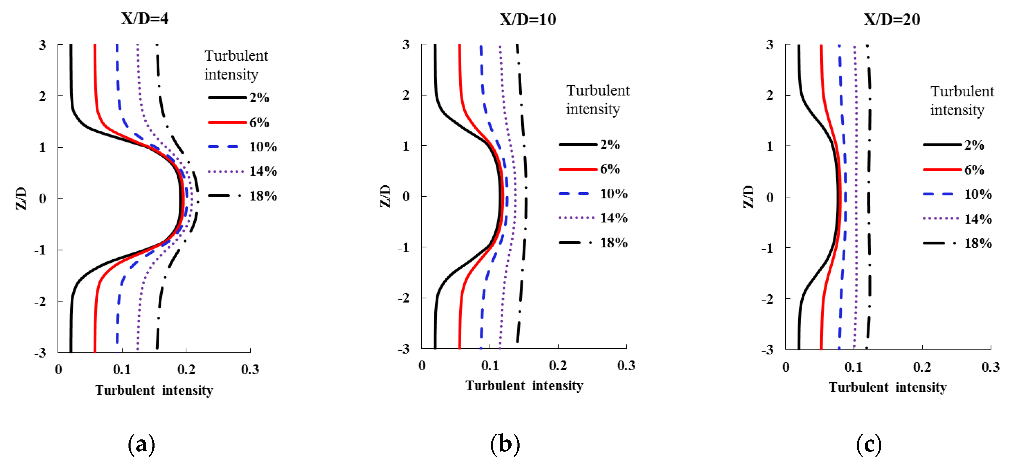
Figure 10.
Analytical wake model results against CFD data.
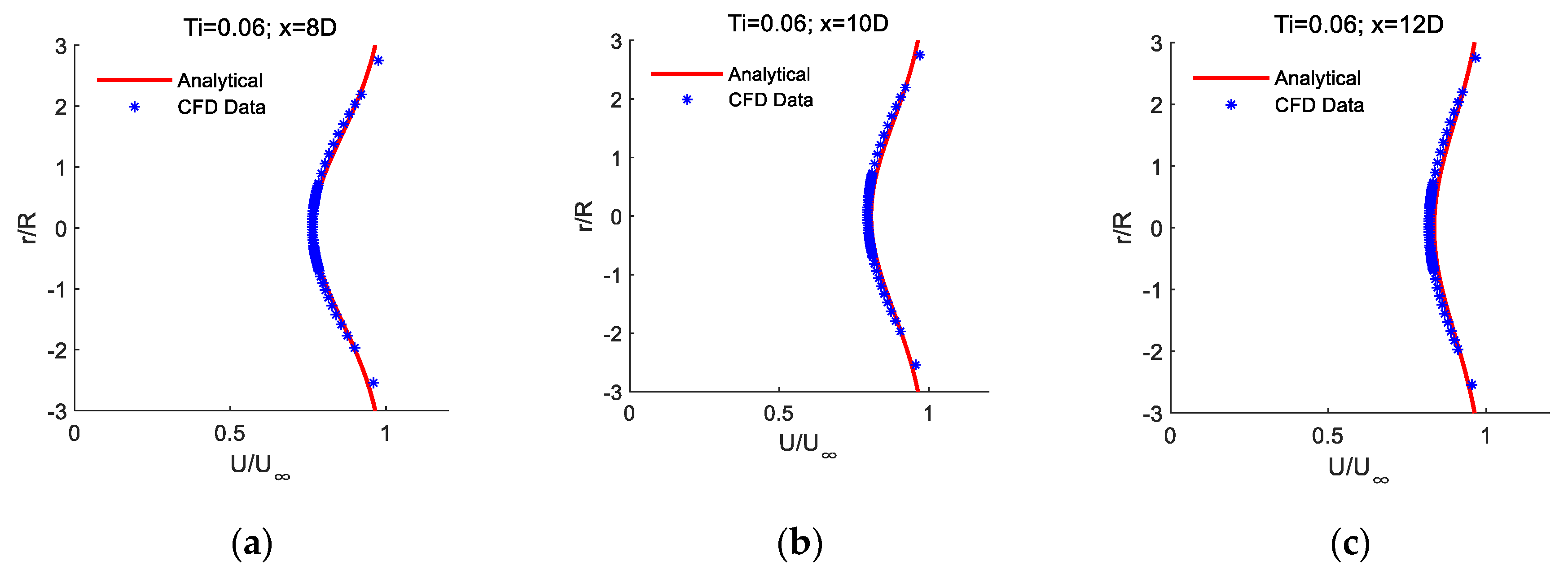

Table 1.
Computational fluid dynamic (CFD) model parameters.
| Parameter | Setting |
|---|---|
| Solver | Pressure-Based |
| Fluid of domain | Incompressible water |
| Turbulence model | SST |
| Time Solution | Steady |
| Inlet; Outlet | Velocity Inlet; Pressure Outlet |
| Top | Slip Wall |
| Bottom and Outside | Wall |
| Convergence criteria | Residual 1×10⁻³ |
Table 2.
Results of mesh independence study.
| Case | Number of mesh nodes | Deficit of centerline at 8D of simulation | ||
|---|---|---|---|---|
| 01 | 5.1*106 | 0.241 | 0.205 | 0.041 |
| 02 | 6.3*105 | 0.242 | 0.210 | 0.042 |
| 03 | 3.2*105 | 0.255 | 0.275 | 0.055 |
Table 3.
Error analysis.
| Line | Deficit(X/D=4) | Deficit(X/D=8) | Deficit(X/D=12) | |||||||||
|---|---|---|---|---|---|---|---|---|---|---|---|---|
| Sim | Exp | Sim | Exp | Sim | Exp | |||||||
| 01 | 0.53 | 0.38 | 0.39 | 0.15 | 0.24 | 0.2 | 0.20 | 0.04 | 0.14 | 0.11 | 0.27 | 0.03 |
| 02 | 0.51 | 0.35 | 0.46 | 0.16 | 0.24 | 0.22 | 0.09 | 0.02 | 0.13 | 0.11 | 0.18 | 0.02 |
| 03 | 0.46 | 0.26 | 0.77 | 0.2 | 0.21 | 0.18 | 0.17 | 0.03 | 0.12 | 0.09 | 0.33 | 0.03 |
| 04 | 0.35 | 0.22 | 0.59 | 0.13 | 0.19 | 0.15 | 0.27 | 0.04 | 0.11 | 0.09 | 0.22 | 0.02 |
Table 4.
Goodness of fit analysis.
| x/D | Ti = 0.02 | Ti=0.1 | Ti=0.14 | |||
|---|---|---|---|---|---|---|
| R2 | RMSE | R2 | RMSE | R2 | RMSE | |
| 4 | 0.9809 | 0.0030 | 0.9034 | 0.0355 | 0.9944 | 0.005 |
| 6 | 0.8209 | 0.0334 | 0.9927 | 0.0031 | 0.8788 | 0.0193 |
| 8 | 0.8386 | 0.0250 | 0.9865 | 0.0058 | 0.8765 | 0.0138 |
| 10 | 0.9586 | 0.0079 | 0.8958 | 0.0143 | 0.9717 | 0.0045 |
| 12 | 0.9807 | 0.0041 | 0.7861 | 0.0167 | 0.9810 | 0.0022 |
Disclaimer/Publisher’s Note: The statements, opinions and data contained in all publications are solely those of the individual author(s) and contributor(s) and not of MDPI and/or the editor(s). MDPI and/or the editor(s) disclaim responsibility for any injury to people or property resulting from any ideas, methods, instructions or products referred to in the content. |
© 2025 by the authors. Licensee MDPI, Basel, Switzerland. This article is an open access article distributed under the terms and conditions of the Creative Commons Attribution (CC BY) license (http://creativecommons.org/licenses/by/4.0/).
Copyright: This open access article is published under a Creative Commons CC BY 4.0 license, which permit the free download, distribution, and reuse, provided that the author and preprint are cited in any reuse.


