Submitted:
13 December 2025
Posted:
16 December 2025
You are already at the latest version
Abstract
Entropy appears in physics in many forms—thermal, quantum, informational, gravitational—yet its conceptual foundations remain disparate. We propose a unified definition of entropy grounded in global physical constraints. A constraint set C determines the admissible microstate region Γ(C), and the entropy is defined as S(C) = kBlnVol[Γ(C)]. This constraint–volume formulation applies uniformly to classical and quantum systems, to internal and external degrees of freedom, and to finite or continuous state spaces, without invoking coarse-graining, ensembles, or subjective information. Local interactions generically weaken global constraints such as coherence, correlations, gradients, and entanglement structure. We prove a structural Second Law: whenever constraints decay under dynamical evolution, C(t +∆t) ⊆ C(t), the entropy must increase. This mechanism explains thermodynamic irreversibility, decoherence, thermalization, and hydrodynamic mixing as manifestations of constraint erosion, while identifying integrable and symmetry-protected systems as the exceptional cases in which constraints persist. The framework clarifies how macroscopic entropy can grow evenwhenmicroscopic dynamics are reversible, and why time itself is not a form of entropy. Classical thermodynamic entropy, quantum von Neumann entropy, and black hole entropy all emerge as special cases of the same structural principle.
Keywords:
constraint–volume entropy
; global constraints
; constraint decay
; second law of thermodynamics
; irreversibility
; decoherence
; entanglement entropy
; Von Neumann entropy
; Boltzmann entropy
; thermalization
; quantum chaos
; hydrodynamic relaxation
; microscopic reversibility
; entropy production
1. Introduction
Entropy appears throughout physics in multiple forms.1 Each formulation is mathematically precise within its own domain, yet the physical meaning of “entropy” and the origin of the Second Law remain conceptually unsettled. Is entropy a measure of disorder, missing information, spatial mixing, quantum entanglement, coarse-graining, or something else? The existence of many definitions has encouraged the view that “entropy” is inherently context-dependent and must be reinterpreted in each subfield [7].
In this work we propose a unified conceptual and mathematical foundation for entropy based on a simple structural insight: every entropy notion in physics counts the number of microstates compatible with a given set of global physical constraints. These constraints may be internal (quantum coherence relations, entanglement structure, stabilizer conditions) or external (spatial gradients, macroscopic correlations, hydrodynamic fields), but they play the same logical role: each constraint restricts the allowable relationships among the system’s degrees of freedom, and the intersection of all surviving constraints determines the admissible microstate region.
Let C denote the system’s current global constraints. The associated admissible microstates form the region
where X is the full kinematic state space appropriate for the system [8,9]. The constraint volume
counts these microstates, and the entropy
measures the size of this constraint-defined region. This definition recovers the Boltzmann entropy (external macroscopic constraints), the von Neumann entropy (internal quantum constraints), coarse-grained entropies, and all standard equilibrium ensembles as special cases [8,10]. It does so without invoking subjective information, arbitrary coarse-graining, or preferred subsystem partitions.
A second key observation is dynamical. In physically realistic, non-integrable systems with local interactions, global constraints generically decay over time. Internal constraints—such as phase coherence and entanglement structure—are degraded by decoherence [11], scrambling, eigenstate thermalization [12,13], and quantum chaos [14]. External constraints—such as spatial correlations and macroscopic gradients—are weakened by mixing, diffusion, turbulence, and classical chaos [15]. Although integrable or symmetry-protected models preserve special constraint structures, these represent a measure-zero subset of Hamiltonians and do not describe generic matter.
For almost all physical systems, microscopic interactions enlarge the set of compatible microstates over time:
This purely structural implication is formalized as the Constraint Monotonicity Theorem. It yields an objective, model-independent form of the Second Law: entropy increases because local interactions erode global consistency relations.
This perspective resolves a longstanding conceptual misunderstanding: time is not entropy. Time orders physical states; entropy measures the volume of microstates compatible with the present constraint structure. Microscopic evolution (Hamiltonian or unitary) is reversible, and nothing in the definition of entropy requires monotonicity. Entropy growth is instead a contingent consequence of the generic weakening of global constraints, absent special symmetries or integrable structures [16].
The goal of this paper is to develop this constraint-based foundation for entropy in a precise and unified manner. Our main contributions are:
- We introduce a general definition of entropy as the logarithmic volume of microstates compatible with the system’s surviving global constraints, treating internal and external degrees of freedom on equal footing.
- We identify the dynamical mechanism responsible for entropy increase in realistic physical systems: local interactions generically weaken global constraints, thereby enlarging the admissible microstate region.
- We prove a structural Second Law (Constraint Monotonicity Theorem), demonstrating that constraint weakening necessarily increases entropy, independently of coarse-graining or subjective information.
- We recover classical thermodynamic entropy and equilibrium ensembles as limiting cases that emerge once internal coherence constraints have fully decayed.
- We show through explicit examples how the unified framework describes entropy increase in quantum systems (decoherence, entanglement decay), classical systems (mixing, diffusion), and hybrid systems (melting, turbulent relaxation).
- We clarify the conceptual distinction between time and entropy, showing that irreversibility arises from the erosion of global constraints rather than from any intrinsic temporal asymmetry.
The remainder of the paper is organized as follows. Section 2 defines global constraints and introduces the associated microstate sets. Section 3 presents the constraint-volume definition of entropy. Section 4 analyzes the physical mechanisms by which global constraints decay under generic local dynamics. Section 5 proves the Constraint Monotonicity Theorem. Section 6 shows how classical thermodynamics emerges as a special case. Section 7 applies the framework to quantum entropy and decoherence. Section 8 provides illustrative examples across internal, external, and hybrid systems. Section 9 discusses integrability and other exceptions. Section 10 clarifies why time is not entropy. We conclude in Section 11 with conceptual implications and future directions. Technical details are collected in the appendices.
2. Global Constraints as the Foundation of Entropy
Entropy, in every domain of physics, quantifies the size of the microstate space compatible with the macroscopic or mesoscopic conditions that the system currently satisfies [10]. These conditions—energy conservation, spatial organization, quantum coherence patterns, symmetries, topological relations, or environmental couplings—all take the mathematical form of constraints. This section formalizes the notion of a global constraint, explains its physical motivation, and introduces the associated microstate sets that will underlie the definition of entropy.
See Appendix A for the formal structure of constraints.
2.1. Global Constraints: Definition and Motivation
A physical system with degrees of freedom X (which may be classical, quantum, or hybrid) does not typically explore the entirety of its kinematic space. Its admissible configurations are restricted by a variety of global constraints, which may arise from physical laws, environmental couplings, or dynamical history [8].
These constraints fall into two broad categories:
Internal constraints.
These involve relations among internal, often non-spatial, degrees of freedom. Examples include:
Internal constraints determine which quantum states, reduced density matrices, stabilizer configurations, or internal polarization patterns the system may occupy. Decoherence and quantum chaos [14] typically degrade these constraints over time.
External constraints.
These involve relations among spatial or macroscopic degrees of freedom. Examples include:
- macroscopic density distributions or gradients,
- velocity fields and hydrodynamic profiles,
- geometric arrangements or spatial correlation structures,
- boundary conditions or conserved macroscopic moments,
- large-scale order (e.g. crystalline, liquid, or flocking structures).
External constraints describe the macroscopic organization of mass, energy, momentum, and spatial correlations. They are degraded by diffusion, mixing, turbulence, classical chaos, and hydrodynamic relaxation [15].
Despite appearing fundamentally different, both internal and external constraints share the same logical role: they restrict the admissible microstates of the system. It is this restriction—not the specific nature of the degrees of freedom—that entropy quantifies.
2.2. Constraint Sets and Admissible Microstates
Let X denote the kinematic microstate space of the system (phase space in the classical case, or a Hilbert space or operator algebra in the quantum case). A global constraint restricts the system to a subset of X. Multiple constraints narrow this subset via intersection [8].
Definition 1.
A constraint set C is a collection of global relations among the degrees of freedom of a physical system. The corresponding set of compatible microstates is
Thus:
- adding a new constraint shrinks ,
- removing a constraint enlarges ,
- and the admissible microstate space is fully determined by the intersection of all relations in C.
2.2.0.3. Examples.
- In a dilute classical gas, C may specify the total energy, particle number, and the absence of macroscopic gradients. Then is the usual microcanonical shell of phase space [8].
- In a quantum measurement scenario, C may encode the preserved branch structure or pointer observables. Removing internal coherence constraints enlarges to include decohered mixtures [11].
- In a many-body quantum system, C might impose stabilizer relations or entanglement conditions. Scrambling dynamics weaken these, enlarging the set of compatible density matrices.
- In a macroscopic fluid, C may include hydrodynamic simplifications or macroscopic organization. Turbulence and mixing degrade these constraints, enlarging .
This formalism applies uniformly across classical and quantum mechanics, with the only difference being the nature of the underlying space X.
2.3. Constraint Weakening and Physical Evolution
Physical dynamics typically act locally: interactions couple degrees of freedom within finite spatial range or finite circuit depth [9]. Such local interactions do not, in general, preserve global relations. Instead, they tend to weaken or destroy global constraints unless symmetry-protected.
Let denote the constraint set satisfied at time t. For generic, non-integrable systems, we typically have
meaning some global relations no longer hold at later times. This inclusion expresses the physical fact that global coherence, long-range organization, or macroscopic regularity are eroded by local microscopic interactions.
At the microscopic level, internal constraints are degraded by:
At the macroscopic level, external constraints are degraded by:
The only exceptions are highly structured, fine-tuned systems: many-body localized phases [17]. These systems preserve special global constraints but constitute a measure-zero subset of physically relevant models. In all realistic interacting systems, constraint weakening is the generic outcome of dynamical evolution.
This monotonic reduction of constraints will form the basis for the structural Second Law established in the next section.
For a formal treatment of constraint sets under dynamical evolution, see Appendix F.2.
2.4. Mathematical Assumptions and Scope
The structural results developed in this work rely on a small set of standard assumptions about state spaces, measures, and constraint sets. For clarity, we summarize them here.
1. Measurable state space.
2. Measurable constraints.
Each constraint c selects a measurable set , and constraint sets are countable families with admissible region
Measurability of intersections is assumed.
3. Finite or normalized admissible volume.
Whenever the absolute entropy
is used, we assume
For infinite-dimensional or continuous systems where volumes diverge, all physical quantities are defined either through:
- ratios of volumes (entropy differences),
- finite-volume regularization on spatial domains, or
- normalized reference measures (see Appendix C for details).
This guarantees that every logarithm appearing in the main text is well-defined.
4. Continuity under parameter perturbations.
5. Dynamical evolution of constraints.
For a measurable semigroup , dynamical updates of constraints are defined by pullback,
We assume that is measurable (and measure-preserving when required), ensuring that admissible volumes remain well-defined.
6. Asymptotic regions.
When analyzing long-time behavior, asymptotic constraint sets
are assumed nonempty and measurable (guaranteed when X is compact or when is mixing/ergodic with a unique invariant measure; see Appendix F).
7. Integrable systems as boundary cases.
Integrable systems are characterized by conserved quantities whose level sets have finite, nonzero measure; for such systems the admissible region is invariant, and remains constant.
These assumptions are mild, standard in statistical mechanics and quantum information theory, and sufficient to guarantee that all volume, entropy, and constraint-evolution relations appearing in the main text and appendices are mathematically well-defined.
3. Constraint–Volume Entropy
Entropy quantifies the size of the microstate set compatible with the system’s surviving global constraints [7,10]. Once a constraint set C and its admissible region are specified, the entropy follows directly from the volume of that region. This section introduces the formal definition and explains how it provides a unified foundation for every major notion of entropy in physics.
3.1. Definition of Constraint–Volume Entropy
Let X denote the kinematic microstate space of a physical system. Depending on context, X may be:
Given a constraint set C, the admissible microstate manifold is
Because constraints restrict the allowable relations among degrees of freedom, is generally a strict subset of X.
Definition 2
This definition is coordinate-free and physically objective: entropy depends only on the measure of the admissible region of state space, not on any particular parametrization. The volume measure is chosen to respect the symmetries of the underlying theory (Hamiltonian invariance in classical mechanics, unitary invariance in quantum theory), ensuring that reflects intrinsic physical structure.
Systems with many intact constraints have small admissible sets and therefore low entropy; systems in which constraints have weakened or been destroyed have large admissible sets and correspondingly high entropy.
For continuous or infinite-dimensional systems (e.g. classical fields or quantum fields), volumes require ultraviolet and infrared regularization. A systematic treatment is given in Appendix D (see also for field-theoretic background).
Figure 1 illustrates the geometry of constraint sets: as constraints decay under generic local dynamics, the admissible region expands and the constraint–volume entropy increases.
3.2. Relation to standard entropy notions
Although the expression resembles the familiar Boltzmann entropy, the definition given here is significantly more general and subsumes all major entropy concepts in physics.
Boltzmann entropy (classical external DOFs).
If C specifies macroscopic constraints such as fixed energy, volume, and particle number, then coincides with the corresponding energy shell or macrostate region of classical phase space. The constraint–volume entropy reduces to the usual Boltzmann entropy [19],
Gibbs–Shannon entropy.
von Neumann entropy (quantum internal DOFs).
When X is the space of density matrices and C encodes all linear constraints defining a given density operator (trace 1, positivity, specified reduced states), the constraint volume becomes the measure of all purifications or all internal states compatible with those constraints. In the continuum limit, this recovers von Neumann entropy [20].
Entanglement entropy.
If C specifies fixed reduced density matrices for subsystems or fixed entanglement constraints, then is the space of pure states with those marginals. Its volume reproduces the entanglement entropy of the subsystem, as established in geometric derivations of bipartite entanglement measures [3].
Coarse-grained and hydrodynamic entropy.
Macroscopic fields, such as density distributions or velocity profiles, define constraints on the microscopic configuration. The volume of microstates compatible with these fields yields the coarse-grained entropy used in nonequilibrium statistical mechanics and hydrodynamics [21].
Black-hole and horizon entropy.
Geometric horizon constraints restrict admissible spacetime or quantum gravitational microstates. The Bekenstein–Hawking entropy can be interpreted as the logarithm of the volume of microstates compatible with these geometric constraints [4,5], placing horizon entropy within the same framework.
Thus the constraint–volume entropy unifies classical, quantum, information-theoretic, and gravitational entropies within a single mathematical object: the volume of admissible microstates.
The subtleties associated with infinite-dimensional configuration spaces and their regularization are addressed in Appendix D.
3.3. Novelty of the Constraint–Volume Viewpoint
The novelty of the present framework is not the expression itself, which dates back to Boltzmann [19], but rather the recognition that entropy always counts microstates compatible with the system’s current global constraints, regardless of whether these constraints are:
- internal or external,
- quantum or classical,
- microscopic, mesoscopic, or macroscopic,
- spatial, algebraic, topological, or coherence-based.
In standard treatments, different entropies arise from different interpretations of and from different types of constraints: Boltzmann’s entropy uses macroscopic external constraints; von Neumann entropy uses subsystem constraints; entanglement entropy uses reduced state constraints; coarse-grained entropy uses spatial averaging constraints; and information-theoretic entropy uses probabilistic constraints [7,9].
Here all of these disparate notions are unified by the simple structural statement:
This viewpoint eliminates the need for:
It also sets the stage for the structural Second Law derived in the next section: since local interactions generically degrade global constraints, the admissible microstate volume grows monotonically, leading to the objective increase of entropy.
4. Dynamics: Why Global Constraints Decay
Global constraints encode nonlocal relations among the degrees of freedom of a system [22]. These relations may correspond to spatial organization, quantum coherence [11], entanglement patterns, stabilizer conditions, hydrodynamic fields [21], or symmetry constraints. Physical interactions, however, are typically local: they couple degrees of freedom only within finite spatial ranges or finite circuit depths [23]. Local interactions do not generically preserve global structure. Instead, they tend to weaken or destroy it unless protected by special symmetries. This section explains, in a unified manner, the dynamical mechanisms responsible for the generic decay of global constraints in both internal and external degrees of freedom.
Figure 2 illustrate how local dynamics disrupts constraints.
4.1. Internal Degrees of Freedom
Internal degrees of freedom include quantum phases, coherence relations, entanglement structure, reduced density matrices, stabilizer conditions, spin correlations, and algebraic relations among subsystem states. These internal constraints are highly sensitive to the system’s local dynamics [9].
For quantitative timescales governing the decay of these internal constraints, see Appendix E.
Decoherence.
A system interacting with an environment undergoes decoherence: phases between different pointer states are rapidly suppressed [11], reducing the set of compatible pure states. The constraint set loses coherence-based relations, and enlarges accordingly.
Entanglement scrambling.
Unitary evolution under generic many-body Hamiltonians spreads quantum information across the system. Initially localized correlations become delocalized, and subsystem constraints (fixed marginals or purity) are weakened.
Eigenstate Thermalization (ETH).
For non-integrable quantum systems, ETH implies that the reduced state of almost any late-time subsystem becomes indistinguishable from the microcanonical ensemble [12,13]. This corresponds to the loss of detailed internal correlations and the replacement of strict constraints with coarse macroscopic ones.
Quantum chaos.
Underlying both scrambling and ETH is quantum chaos: exponential sensitivity to perturbations and rapid mixing in Hilbert space [14]. Quantum chaos erodes fine-grained coherence constraints, increasing the admissible microstate volume.
In all these cases, internal constraints are fragile: even weak local interactions typically disrupt the relations defining them.
4.2. External Degrees of Freedom
External degrees of freedom include spatial distributions, density gradients, velocity fields, geometric ordering, macroscopic shapes, correlation structures, and momentum-space organization. Local microscopic interactions degrade these constraints through several universal dynamical mechanisms [15].
For quantitative timescales governing the decay of these external constraints, see Appendix E.
Diffusion and transport.
Particle collisions or hopping processes smear out spatial density gradients [24]. As diffusion acts, structured configurations become more uniform.
Mixing.
In classical Hamiltonian systems and deterministic flows, mixing dynamics exponentially stretch and fold phase-space volumes [15]. Macroscopic correlations are destroyed.
Turbulent cascades.
In fluid dynamics, turbulent cascades break down coherent macroscopic flow structures. Vorticity fields become randomized.
Hamiltonian chaos.
Chaotic Hamiltonian dynamics cause exponential divergence of trajectories, erasing simple spatial or momentum-space relations.
Gravitational relaxation.
In astrophysical systems, N-body interactions relax macroscopic structures toward virial equilibrium, erasing detailed correlations.
External constraints are robust at short times but generically decay under nonlinear interactions, transport processes, or chaotic flows.
4.3. Integrable and Symmetry-Protected Exceptions
Although global constraints generically decay, exceptions exist. These exceptions illuminate rather than undermine the mechanism behind constraint decay.
Integrable cases are detailed in Appendix B.
Integrable systems.
Classical integrable systems possess as many conserved quantities as degrees of freedom. Quantum integrable systems possess extensive sets of commuting integrals of motion. These additional constraints prevent mixing, scrambling, or thermalization.
Many-body localization (MBL).
In MBL phases, disorder induces an extensive set of quasi-local conserved quantities [17], preventing the spreading of entanglement.
Symmetry-protected or topologically protected subspaces.
Certain constraints cannot be broken by local interactions due to symmetry or topology.
Measure-zero character.
Integrable and protected systems constitute a measure-zero subset of Hamiltonians: perturbations typically break the additional constraints.
4.4. Unified Mechanism of Constraint Decay
Despite differences between internal and external degrees of freedom, the mechanism of constraint decay is universal:
Local interactions propagate information only within finite ranges and do not generically preserve global relations. Consequently, global constraints decay unless protected by special symmetries.
Internal constraints—coherence, entanglement structure, stabilizer relations—are eroded by scrambling, decoherence, and chaotic unitary dynamics. External constraints—spatial distributions, hydrodynamic fields, macroscopic gradients—are eroded by transport, mixing, turbulence, and classical chaos.
In both cases:
so the admissible microstate volume expands. This monotonicity forms the basis of the structural Second Law proven in the next section.
See Figure 3 for a schematic illustration.
5. The Constraint Monotonicity Theorem (The Second Law)
The central claim of this framework is that entropy increase in physical systems is a structural consequence of the weakening of global constraints under generic local dynamics. In this section we make this statement precise. The result does not depend on statistical assumptions, coarse-graining, or probabilistic interpretation [7]. It follows solely from the set-theoretic relation between constraint sets and the admissible microstate volumes that they define.
5.1. Statement of the Theorem
Let denote the set of global constraints satisfied by the system at time t, and let
be the corresponding admissible microstate set. The structural Second Law follows from the monotonicity of under constraint inclusion [25].
Theorem 5.1
(Constraint Monotonicity). If physical evolution from time t to time weakens the global constraint set, meaning
then the constraint–volume entropy satisfies
with equality if and only if the constraints are unchanged.
Before proving the theorem, it is useful to restate the inclusion condition in physical terms. The relation means that some global relations no longer hold at the later time. Equivalently, the system is compatible with a larger set of microstates than before.
A full proof of the monotonicity of constraint volumes is provided in Appendix F.1.
5.2. Proof of the Theorem
Proof.
If , then any microstate satisfying all constraints in C necessarily satisfies all constraints in . Thus the admissible microstate sets satisfy
Setting and yields the desired result. □
This completes the structural derivation of the Second Law: entropy cannot decrease when global constraints are weakened.
Details of the proofs are presented in Appendix F.
5.3. Interpretation and Physical Significance
The Constraint Monotonicity Theorem identifies the Second Law as an order-theoretic statement. It is not a probabilistic law, nor is it tied to coarse-graining or ignorance; instead, it expresses a purely mathematical relation:
Entropy increases precisely when the system becomes compatible with a strictly larger set of microstates.
Local microscopic interactions tend to destroy global relations, so in almost all realistic systems the constraint set weakens over time, and entropy correspondingly increases [22].
Appendix E analyzes the characteristic timescales associated with constraint decay and the resulting entropy production rates.
5.4. Corollaries
The theorem has several immediate and important consequences.
1. No coarse-graining is required.
The proof uses no approximation or averaging procedure. Entropy increase follows from the weakening of actual physical constraints, not from smoothing out fine details.
2. No subjective information is invoked.
Unlike informational interpretations of entropy, the present framework does not depend on an observer’s knowledge or ignorance [10]. The entropy is an objective property of the constraint structure.
3. The subsystem decomposition is irrelevant.
Because C is defined independently of any particular partitioning of the system, the entropy does not rely on tracing out degrees of freedom.
4. Reversibility vs. irreversibility.
5. Equality conditions.
The entropy is constant during intervals for which , i.e. when the dynamics preserve the constraint set. This occurs in integrable, many-body localized, or symmetry-protected systems and represents the precise boundary case of the Second Law [17].
5.5. Summary
The Constraint Monotonicity Theorem identifies the Second Law of thermodynamics as a mathematical consequence of two facts:
- (1)
- The system’s admissible microstate space is determined by its surviving global constraints.
- (2)
- Generic local interactions weaken global constraints over time, enlarging the admissible microstate space.
Entropy increase therefore arises universally in realistic physical systems, independently of coarse-graining, statistical assumptions, or subjective uncertainty. It is the structural signature of constraint decay. See Figure 4.
6. Classical Thermodynamics as a Special Case
The previous sections established entropy as the logarithmic volume of microstates consistent with the system’s global constraints. In general, these constraints involve both internal degrees of freedom (e.g., quantum coherence relations, entanglement structure) and external degrees of freedom (e.g., spatial correlations, macroscopic gradients). Classical thermodynamics corresponds to a regime in which all internal constraints have decayed, due to rapid decoherence and entanglement scrambling, while the remaining significant constraints are purely external and macroscopic.
In this section we show that, under these conditions, the constraint volume reduces to familiar expressions from equilibrium statistical mechanics [8], including the Boltzmann entropy [19], the microcanonical ensemble, and the canonical ensemble [10]. We also explain how hydrodynamic behavior emerges from constraint decay in macroscopic fields.
6.1. Reduction to Macroscopic External Constraints
Let denote internal coherence or entanglement constraints, and let denote macroscopic external constraints such as total energy, particle number, total momentum, or conserved spatial moments. In generic macroscopic systems, decoherence and quantum scrambling drive
leaving only external constraints relevant at thermodynamic timescales. Thus the full constraint set reduces to
Global correlations encoded in are far more robust than internal quantum constraints, but they too eventually decay through diffusion, mixing, and hydrodynamic relaxation.
In this regime the admissible microstate set is
and the constraint-volume entropy reduces to the Boltzmann entropy when specifies the usual macroscopic variables [19].
6.2. Recovery of the Boltzmann Entropy
Suppose specifies energy E, particle number N, volume V, and possibly total momentum P or angular momentum L. Then
is the classical energy shell of phase space, defined through Liouville’s measure [18]. The microcanonical volume is
Thus the constraint–volume entropy becomes
the standard Boltzmann entropy [19]. No coarse-graining or probabilistic assumptions are required: the external constraints directly determine the measure of admissible states.
6.3. Emergence of Equilibrium Ensembles
Equilibrium ensembles arise naturally from constraint weakening. As the system interacts weakly with an environment or a large reservoir, the constraint set changes:
- If both energy and particle number fluctuate with fixed means, gives the grand canonical ensemble.
- If spatial gradients decay, loses spatial-structure constraints, driving the system toward uniform equilibrium [21].
Formally, if the environment imposes weak constraints on mean values of observables ,
the maximum allowable constraint volume corresponds to the Gibbs distribution [8]
which is the unique state maximizing subject to the remaining constraints [10].
Thus classical equilibrium distributions are the maximizers of the constraint–volume entropy given the set of surviving macroscopic constraints.
6.4. Gas Expansion: Constraint Decay in External DOFs
A simple and illustrative example is the free expansion of a dilute gas initially confined to a subvolume of a larger container of volume . Let encode the spatial constraint that all particles are located within :
At early times the constraint is strong, and
is a small subset of the full phase space.
When the partition is removed, microscopic collisions and ballistic motion rapidly weaken the spatial constraint. After a characteristic diffusion time, the constraint set reduces to
and
is now the full microcanonical shell on the larger volume.
Because
the constraint–volume entropy increases by
the standard textbook result.
This example illustrates how classical thermodynamic irreversibility arises from the decay of spatial external constraints due to microscopic local interactions.
6.5. Hydrodynamic Relaxation and Constraint Decay
Nonequilibrium macroscopic fields such as density and velocity impose constraints on microscopic configurations:
Transport processes, mixing, and viscosity degrade these constraints, driving and toward homogeneous equilibrium values.
Hydrodynamically, this corresponds to the Navier–Stokes or diffusion equations, which monotonically reduce spatial gradients [21]. In the constraint–volume picture, this reduction corresponds to
and thus
Hydrodynamics therefore arises as the macroscopic manifestation of constraint decay in external degrees of freedom. Entropy increase in fluids, plasmas, and gases is the direct structural consequence of this decay.
A detailed analysis of hydrodynamic and mixing timescales appears in Appendix E.
6.6. Summary
Classical thermodynamics emerges naturally from the constraint–volume framework when internal coherence constraints have decayed and only macroscopic external constraints remain. In this limit the constraint–volume entropy reduces to the Boltzmann entropy, and equilibrium ensembles arise as maximizers of the entropy subject to the surviving external constraints. Hydrodynamic relaxation and macroscopic irreversibility correspond directly to the decay of external constraints under local microscopic dynamics. See Figure 5.
7. Quantum Entropy, Decoherence, and Internal DOFs
Quantum systems possess internal degrees of freedom—coherence phases, entanglement patterns, stabilizer relations, operator expectations, and subsystem correlations—that define global constraints on the quantum state [9]. In contrast to macroscopic spatial constraints, internal quantum constraints are highly fragile: they are rapidly degraded by environment coupling and decoherence [11,26], entanglement scrambling [12,13], and generic unitary dynamics in non-integrable many-body systems [27,28]. In this section we show how quantum entropy increase emerges directly from the weakening of these internal constraints.
We also show that subsystem entropy—including the von Neumann and entanglement entropies—arises as a special case of constraint–volume entropy. Appendix C discusses the von Neumann case in detail [29,30].
7.1. Quantum Constraints and Admissible States
Let X be the space of quantum states of a system, typically represented by density matrices on a Hilbert space [9,31]. A quantum constraint is any algebraic or geometric relation on that restricts the allowed set of states. Examples include:
- fixed expectation values: ,
- fixed reduced states: ,
- purity or rank constraints: ,
- coherence constraints: fixed off-diagonal elements,
- entanglement constraints: fixed Schmidt spectra or stabilizers [3].
Given a constraint set C, the admissible quantum states are
When internal constraints decay, enlarges and the constraint–volume entropy increases.
7.2. Decoherence as Constraint Decay
Decoherence is the process by which off-diagonal elements of the density matrix in a preferred basis are suppressed by coupling to an environment, a mechanism extensively analyzed in [11,26,32]. This corresponds to removing phase-coherence constraints.
Let denote the constraints enforcing fixed coherence phases between basis states. Before decoherence,
7.3. Entanglement Scrambling and Subsystem Entropy
Entanglement scrambling refers to the spread of initially localized quantum correlations throughout the system under generic many-body unitary dynamics. This phenomenon underlies quantum thermalization through ETH [12,13,28].
Let denote constraints fixing the reduced density matrix of a subsystem A:
These constraints specify which global states remain compatible with a fixed set of subsystem correlations.
Under generic non-integrable evolution [12,13,27],
because entanglement with B changes . Thus grows and the constraint–volume entropy increases.
When fixes subsystem purity or specific Schmidt coefficients, scrambling drives toward the thermal or Page-typical state, increasing the subsystem entropy [3]. Hence the usual growth of von Neumann entropy is a manifestation of the general structural theorem.
7.4. Loss of Purity as Constraint Removal
Pure states satisfy the stringent algebraic constraint
which restricts the state space to a measure-zero manifold of density matrices [9,33]. Under decoherence or system–environment coupling [11,32], the state becomes mixed:
and the purity constraint is removed:
This dramatically enlarges the admissible microstate set, because mixed states occupy exponentially larger volumes in the space of density operators [29].
Thus the transition from pure to mixed states, often described as loss of information, is precisely a weakening of algebraic constraints.
7.5. Subsystem Entropy as Constraint–Volume Entropy
Consider a bipartite system with Hilbert space . Fixing imposes the global constraint set
The admissible global states form the fiber
The geometry and induced measures of these fibers are well understood [29,30,34]. Their volumes scale as
where is the von Neumann entropy. Thus:
Subsystem (entanglement) entropy is exactly the constraint–volume entropy associated with fixing the reduced state.
This unifies quantum entanglement entropy with classical entropy within a single geometric definition.
7.6. Two-Qubit Example
To illustrate, consider two qubits in the maximally entangled Bell state. The global state is pure, and the reduced states have maximal entropy [3]. Environmental dephasing [32] destroys coherence, removing those internal constraints. Purity is lost, and the admissible microstate region expands. The subsystem entropies then evolve consistently with standard open-system dynamics [11,26,32].
7.7. Summary
Quantum entropy increase—including decoherence, loss of purity, growth of subsystem entropy, and entanglement decay—arises from the decay of internal global constraints. Thus quantum entropy fits seamlessly into the constraint–volume framework, and the structural Second Law applies equally to quantum and classical systems.
See Figure 6 for illustration.
8. Examples of Constraint Decay
The general mechanism of entropy increase established above is the weakening of global constraints under local physical dynamics. In this section we illustrate the framework with several canonical examples spanning quantum, classical, and gravitational systems. Each example demonstrates the same pattern:
- (1)
- Identify the initial global constraints .
- (2)
- Identify the physical mechanism that weakens them.
- (3)
- Show how the admissible microstate space expands.
- (4)
- Conclude that the constraint–volume entropy increases.
These examples jointly demonstrate that the constraint–decay mechanism is not limited to any specific domain of physics, but is a universal structural feature of dynamical systems with local interactions.
8.1. Example 1: Two-Qubit Entanglement Decay
Consider two qubits A and B initially prepared in the Bell state
a standard maximally entangled state. At , the constraint set includes:
- pure-state constraint: ,
- coherence constraint: fixed relative phase between 00 and 11,
- entanglement constraint: fixed Schmidt spectrum,
- subsystem constraint: .
Let qubit B undergo dephasing through a channel , a standard CPTP map generated by phase damping. This removes phase coherence and breaks the entanglement structure.
Thus
and hence
As coherence constraints and purity constraints weaken, the constraint–volume entropy increases monotonically.
8.2. Example 2: Mixing gas in a Box
Consider a gas initially confined to the left half of a box. At time , the global constraints include:
- spatial constraint: all particle positions lie in ,
- macroscopic density gradient: fixed density distribution,
- momentum-position correlations induced by the confinement.
A small aperture is opened at , and the particles disperse.
Collisions and free streaming break the spatial constraint, dilute the density gradient, and destroy the correlations characteristic of confinement.
Thus
The admissible microstate set expands from
to
The Boltzmann entropy increase for this process is therefore a direct special case of the constraint–volume formulation [19].
8.3. Example 3: Melting Crystal (Internal + External Constraint Loss)
A crystal at temperature possesses both:
- external constraints: periodic atomic positions forming a lattice with long-range order,
- internal constraints: quantized vibrational normal modes (phonons) with fixed coherence and phase relations.
As the temperature increases toward the melting point, two forms of constraint decay occur:
(1) External constraint decay.
Atomic positions deviate from lattice points, long-range correlations break down, and the subset of microstates satisfying lattice periodicity shrinks dramatically.
(2) Internal constraint decay.
Phonon modes lose coherent phase relations through anharmonic scattering and phonon–phonon interactions, weakening the internal mode constraints.
When melting completes, the crystal structure is completely lost:
and the admissible microstate volume increases from the measure-zero set of ordered configurations to the astronomically larger liquid-phase configuration space.
This example illustrates the simultaneous decay of internal and external constraints.
8.4. Example 4: Turbulent Relaxation
Consider an initially laminar fluid flow with a highly organized velocity field. The initial constraints include:
- global velocity–gradient relations,
- coherent vortex alignment,
- stable macroscopic invariants (e.g. large-scale helicity),
- absence of fine-scale vorticity structure.
As the Reynolds number increases, the flow becomes turbulent. Energy cascades from large to small scales, and vorticity twisting, stretching, and reconnection destroy the global coherence relations.
Thus the constraint set weakens:
The flow becomes compatible with a vastly larger set of velocity fields, especially those with fine-scale structure. The constraint–volume entropy grows monotonically until the flow reaches a statistically steady turbulent state.
This example shows that external continuum-field constraints obey the same structural monotonicity as discrete quantum constraints.
8.5. Example 5: Black Hole Entropy as Horizon Constraints
For a black hole of horizon area A, the Bekenstein–Hawking entropy
quantifies the number of microstates compatible with the existence of a smooth event horizon of area A [4].
In the constraint–volume framework:
Horizon constraint.
The horizon imposes a global geometric constraint:
consistent with the covariant treatment of black hole thermodynamics [35].
Constraint weakening through Hawking radiation.
As Hawking radiation reduces the horizon area,
Thus the microstate volume increases:
and the entropy grows accordingly.
Interpretation.
This connects black hole entropy directly to the constraint–volume formalism: the horizon enforces a global geometric relation whose weakening under Hawking emission enlarges the admissible solution space. Hence black hole thermodynamics is aligned with the same structural mechanism underlying all other entropy increases.
Summary
Each example—quantum decoherence, gas mixing, melting crystals, turbulent flows, and black hole evaporation—demonstrates the same pattern:
This unified explanation reveals constraint decay as the structural foundation of the Second Law across all physical regimes.
9. Exceptions: Integrability and Constraint Preservation
The structural Second Law established earlier shows that entropy increases whenever global constraints decay under local dynamics. However, certain special classes of physical systems preserve large sets of global constraints indefinitely. These systems do not violate the Second Law; rather, they realize the equality case of the Constraint Monotonicity Theorem:
In this section we identify the principal categories of such systems, clarify the sense in which they preserve constraints, and explain why their exceptional behavior does not contradict the general constraint–decay mechanism.
9.1. Integrable Hamiltonians
A classical or quantum Hamiltonian system is integrable if it possesses a complete set of independent conserved quantities in involution, with N equal to the number of degrees of freedom, as in the Liouville–Arnold theorem [36]. In quantum integrability, these conserved quantities may arise from commuting transfer matrices or Lax pairs [37].
These integrals of motion form a global constraint set,
whose defining relations are preserved exactly under the dynamics:
Thus the accessible region of phase space or state space is confined to an invariant torus or conserved manifold, and the constraint–volume entropy remains constant:
Interpretation.
Integrable systems lie precisely on the entropy-conserving boundary of the structural Second Law. Entropy does not increase because no global constraints decay. Thus integrability is not a violation of the Second Law, but a special degenerate case where constraints are preserved by symmetry rather than destroyed by generic interactions.
The precise conditions for constraint preservation in integrable systems are developed in Appendix F.3 and parallel the derivations of invariant tori in classical integrability [38].
9.2. Many-Body Localization (MBL)
Many-body localized systems preserve an extensive set of emergent quasi-local integrals of motion (“ℓ-bits”) [39,40]. Let denote these integrals. An MBL Hamiltonian satisfies
for all sites i, providing a large and stable constraint set,
These constraints prevent the system from thermalizing or scrambling, consistent with the original Basko–Aleiner–Altshuler formulation of MBL [41]. Thus for all t,
and because the constraints are unchanged, the constraint–volume entropy is constant:
Interpretation.
Many-body localization is an instance where internal global constraints are maintained by disorder-induced emergent symmetries. MBL systems are therefore entropy-stable rather than entropy-increasing, but this behavior is fully consistent with the monotonicity theorem.
9.3. Topological Phases and Stabilizer Codes
Topological phases of matter [42] and quantum error–correcting stabilizer codes [43] provide another family of systems where global constraints are protected, but for different reasons: they arise from topological, nonlocal orders rather than integrability.
Let the stabilizers define the code space or ground-state manifold, as in the toric code [44]. These impose the constraints
As long as the system remains below a threshold of thermal or environmental noise, these constraints are preserved:
Thus the admissible microstate space remains fixed and entropy does not increase:
Interpretation.
Topological constraints are stable because local perturbations cannot change the global topological sector. Hence these phases again realize the equality case of the structural Second Law.
9.4. Why These Exceptions Do Not Violate the Second Law
The Constraint Monotonicity Theorem states:
It does not assert that must happen for all systems. Instead, the theorem identifies entropy increase with constraint decay.
The exceptions are systems where is invariant.
Integrable, MBL, and topologically ordered systems preserve because:
- integrable systems have symmetries preventing constraint decay,
- MBL systems have emergent local integrals of motion resisting scrambling,
- topological phases protect global information from local noise.
Thus these systems do not satisfy the hypothesis of constraint weakening, and they naturally realize the boundary case of
The Second Law applies generically, not universally.
Entropy increase is a generic feature of local interacting systems with no protecting symmetries or disorder-induced integral structures. These exceptional systems are measure-zero in Hamiltonian or Liouvillian parameter space [45]. Any perturbation breaking the special structure will cause to decay and entropy to begin increasing.
9.5. Summary
Integrable dynamics, many-body localization, and topological stabilizer structures do not violate the Second Law in the constraint–volume picture. They represent special situations in which:
so the admissible microstate set does not expand and entropy remains constant. These cases lie exactly on the equality boundary of the structural Second Law. In all generic systems without symmetry protection or disorder-stabilized integrals of motion, local interactions necessarily degrade global constraints, and entropy increases.
10. Time Is Not Entropy
Entropy and time are often conflated in informal discussions of the Second Law. Because entropy tends to increase in closed macroscopic systems, it is sometimes suggested that entropy is time, or that the growth of entropy defines the direction or flow of time [46]. In the constraint–volume framework, this identification is neither necessary nor accurate. Time and entropy play fundamentally different roles:
- Time parametrizes the evolution of physical configurations according to microscopic dynamical laws (classical Hamiltonian flow or unitary quantum evolution) [38].
- Entropy is a functional of the system’s current global constraint set C, measuring the volume of microstates compatible with those constraints.
This section clarifies the distinction and shows why the Second Law should be understood as a structural statement about constraint decay, not as an identity between time and entropy.
10.1. Time as a Parameter of Dynamical Evolution
In both classical and quantum mechanics, time enters as a parameter in the dynamical equations:
In both cases, the microscopic dynamics are time-reversal invariant: for each trajectory or state , there exists a reversed trajectory or time-reversed state that is equally allowed by the equations of motion. Nothing in these equations requires entropy to increase or to play any distinguished role in defining time.
10.2. Entropy as a Functional of Constraints
Entropy in this framework is defined by
where C is the current global constraint set and is the corresponding admissible microstate space.
Crucially:
- S is a function of the constraint structure, not of time directly,
- Time enters only through the time-dependence of ,
- If is constant in time, then is constant, regardless of how time evolves [47].
Thus, time and entropy are conceptually orthogonal: time orders states, while entropy measures the size of the set of states compatible with the constraints those states satisfy.
10.3. Microscopic Reversibility and Macroscopic Irreversibility
The Constraint Monotonicity Theorem states that entropy increases when the constraint set weakens:
This is a one-way implication: it does not assert that such weakening must occur along every trajectory.
Microscopic reversibility remains intact:
- For any forward-time evolution from to there exists a time-reversed evolution from back to allowed by the microscopic equations [1].
- Along the reversed evolution, the constraint set may strengthen:leading to a decrease in entropy along that trajectory.
The fact that such entropy-decreasing trajectories exist is the content of Loschmidt-type objections to the Second Law [48,49]. In the constraint–volume framework, these trajectories correspond to fine-tuned evolutions in which global constraints are restored rather than degraded.
Macroscopic irreversibility is explained not by a fundamental asymmetry in the dynamical laws, but by the statistical unlikelihood of such fine-tuned trajectories [50]. For generic initial conditions evolving under local dynamics, global constraints monotonically decay, and entropy increases.
10.4. Entropy Under Time Reversal
Consider a forward evolution from time to :
By the monotonicity theorem, .
Now consider the time-reversed evolution, starting from the microstate at and running backwards to time . From the point of view of the reversed dynamics, the constraint set typically strengthens:
and the entropy decreases along this reversed trajectory.
Thus entropy can increase or decrease under time reversal, depending on the direction in which we follow the trajectory. This confirms that entropy does not define time; rather, it is a directional property of certain physically realized evolutions [46].
Appendix F.4 provides the derivation showing how entropy production arises despite reversible microscopic dynamics.
10.5. Low-Entropy Past and the Arrow of Time
The empirical fact that entropy has been increasing over cosmological and laboratory timescales reflects a contingent boundary condition: the early Universe and the initial states of laboratory systems began in configurations with highly restrictive global constraints and therefore low entropy [50].
Given such low-entropy initial conditions, generic local dynamics will monotonically weaken global constraints and increase entropy. This defines a thermodynamic arrow of time relative to the chosen initial conditions, not an intrinsic identity between entropy and time.
In the constraint–volume framework, the arrow of time emerges from:
- (1)
- an initial constraint set that is unusually strong (small ),
- (2)
- generic local dynamics that weaken for ,
- (3)
- the structural monotonicity .
Time itself, however, is simply the parameter t labeling the dynamical evolution; it has no entropy content.
10.6. Clarifying the Distinction with Examples
Spin-echo experiments.
In spin-echo protocols, an initially ordered spin configuration dephases (constraints decay, entropy increases) and then rephases under a carefully engineered pulse sequence [51]. Time runs forward throughout; entropy first rises, then falls. This shows explicitly that entropy is not identical to time.
Gas compression by external work.
A gas that has spread through a box (high entropy) can be quasi-statically compressed back into a smaller volume by external work, restoring constraints on spatial localization. Entropy decreases in this process, even though time flows forward [8].
Fine-tuned microscopic reversal.
In principle, if all particle velocities in a gas were exactly reversed, the gas would spontaneously recontract and recover its initial constraint structure, reducing entropy [48]. Such trajectories exist but are fantastically improbable.
In all these examples, time evolves uniformly, while entropy may increase, remain constant, or decrease, depending on whether constraints are weakened, preserved, or restored.
10.7. Summary
Time and entropy are fundamentally distinct concepts:
- Time parametrizes dynamical evolution and is symmetric in the microscopic equations.
- Entropy measures the volume of microstates compatible with the system’s global constraint set.
The Second Law, in its structural form, states that entropy increases when global constraints decay under generic local dynamics. This explains the observed thermodynamic arrow of time as a consequence of low-entropy initial conditions and typical dynamical behavior, not as an identity between time and entropy. Entropy is not time; it is a structural measure of constraint loss.
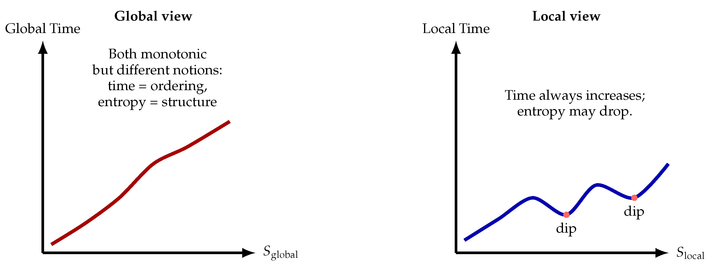
Figure 7.
Time is not entropy. Left: Globally, both time and entropy appear monotonic, but this does not imply identity: time is a relational ordering, while entropy measures the number of microstates compatible with global constraints. Right: Locally the distinction is explicit: entropy may rise or fall, while time always advances. Thus correlation does not imply equivalence.
11. Discussion
The constraint–volume formulation developed in this work provides a unified and conceptually clean foundation for entropy across classical, quantum, and gravitational settings. Similar unifying ambitions appear in earlier approaches to statistical mechanics and thermodynamics [8,10,50,52], but the present framework derives these notions structurally from constraint geometry itself. In this section we discuss the broader implications of the framework, clarify its relationship to existing notions of entropy, and show how it resolves several long-standing conceptual puzzles in thermodynamics, quantum information, and statistical mechanics.
11.1. Entropy as a Structural Property of Constraints
In traditional treatments, entropy is variously interpreted as:
These characterizations differ significantly in meaning and domain of applicability, contributing to persistent confusion about what entropy actually is. In this work we have shown that all these notions arise as special cases of a single structural quantity:
where C is the set of global physical constraints currently satisfied by the system. Entropy is thus an objective, physically grounded measure of the “size” of the admissible microstate space compatible with the system’s global relations.
This resolves longstanding debates about whether entropy is subjective, informational, or statistical [7]. Entropy in this formulation is purely structural: it depends only on the physical constraints that define the system, not on epistemic ignorance or coarse-graining conventions.
11.2. Relation to Jaynes and Maximum Entropy
Jaynes’ maximum-entropy principle posits that one should assign the probability distribution over microstates that maximizes Shannon entropy subject to known macroscopic constraints [10]. In our framework, Jaynes’ principle emerges naturally once one identifies C with the set of known global constraints:
Maximizing the Shannon or von Neumann entropy over this admissible set is equivalent to identifying a representative state that reflects the loss of all other constraints. Thus Jaynes’ variational principle is recovered as the operational rule for selecting a state when C is partially known.
However, the constraint–volume entropy itself is more fundamental: it measures the actual structural freedom of the system, regardless of what an observer knows.
11.3. Relation to Shannon and von Neumann Entropy
Shannon and von Neumann entropies arise from internal degrees of freedom and reflect the decay of internal algebraic constraints such as:
- coherence relations,
- entanglement structure,
- purity constraints,
- subsystem–environment correlations.
In the constraint–volume framework:
- Shannon entropy measures the logarithmic volume of classical distributions compatible with certain informational constraints.
- von Neumann entropy measures the logarithmic volume of quantum states compatible with fixed reduced density matrices or other operator constraints [9].
Thus both appear as special cases of when C fixes probability distributions or density matrices.
11.4. Relation to Decoherence and Emergent Classicality
Decoherence theory explains how quantum systems lose internal phase relations and acquire classical-like behavior via entanglement with their environments [11]. In our formulation, decoherence corresponds to a strict weakening of internal constraints:
as coherence relations and entanglement structures degrade. Thus the growth of subsystem entropy in decoherence is a direct instance of the structural Second Law.
The constraint–volume framework also clarifies the emergence of classical ensembles: they arise when internal quantum constraints have decayed sufficiently that only external macroscopic constraints remain, so the admissible states reduce to classical statistical distributions.
11.5. Relation to Eigenstate Thermalization (ETH)
The Eigenstate Thermalization Hypothesis states that generic, non-integrable quantum systems effectively “self-thermalize” because individual eigenstates already encode thermal correlation functions [12,13,27]. In the constraint–volume picture, ETH corresponds to:
- Generic Hamiltonians degrade internal correlation constraints via unitary scrambling.
- The constraint set becomes dominated by only a few macroscopic conserved quantities (energy, particle number).
- The admissible microstate set becomes essentially the microcanonical shell.
Thus ETH is the dynamical mechanism by which constraint decay removes all fine-grained structure, leaving only robust global conservation laws.
11.6. A Unified Foundation for Entropy
The structural constraint–volume formulation unifies:
- classical thermodynamic entropy,
- quantum entropy and entanglement entropy,
- decoherence-induced entropy growth,
- statistical entropy in probability theory,
- hydrodynamic entropy in continuum systems.
All are examples of the same principle:
This eliminates the need for multiple entropy definitions across physics.
11.7. Resolution of Long-Standing Conceptual Puzzles
This framework dissolves several persistent puzzles:
(1) Why does entropy increase if microscopic laws are reversible?
Because microscopic reversibility only implies that constraint-restoring trajectories exist, not that they are dynamically typical [49]. Generic interactions destroy global constraints; restoring them requires fine-tuning.
(2) Is coarse-graining essential?
No. Coarse-graining is epistemic [10]; constraint decay is physical and structural.
(3) What is the role of information?
Informational interpretations follow when C encodes informational constraints; in general, entropy is objective [7].
(4) Why do classical thermodynamic and quantum entanglement entropies share a form?
Because both quantify constraint loss in their respective state spaces.
(5) How does the arrow of time arise?
From low-entropy initial conditions [50] and the generic decay of global constraints—not from entropy defining time.
11.8. Uniqueness of the Constraint–Volume Framework
The present formulation raises a natural question: could there exist other equally general and physically meaningful definitions of entropy? Many well-established notions of entropy have been proposed—including the Shannon and Gibbs–Shannon entropies [2,10], the von Neumann entropy [20], coarse-grained Boltzmann entropy [1], entanglement entropy in quantum many-body systems [3], and geometric or gravitational entropies such as the Bekenstein–Hawking formula [4,5]. Each is mathematically precise within its domain, yet none provides a single structural principle that applies uniformly across classical, quantum, and gravitational regimes.
A genuinely unified entropy must satisfy several criteria: (i) applicability to classical and quantum systems, including continuous or infinite-dimensional state spaces; (ii) invariance under the natural symmetries of the theory (Liouville invariance [18] in classical mechanics, unitary invariance [9] in quantum mechanics); (iii) recovery of standard thermodynamic, information-theoretic, and quantum entanglement entropies; (iv) compatibility with reversible microscopic dynamics; and (v) independence from subjective information, coarse-graining prescriptions, or arbitrary subsystem decompositions [7].
Information-theoretic entropies depend on observer knowledge; coarse-grained formulations require privileged partitions of phase space; entanglement entropies rely on subsystem boundaries and do not apply outside quantum settings; and gravitational or holographic entropies apply only in special spacetime backgrounds. None of these approaches provides the structural generality or dynamical transparency required for a fully universal Second Law.
By contrast, the constraint–volume definition,
is determined solely by the measure-invariant size of the admissible state-space region defined by the system’s surviving global constraints. Constraints are the only structural mechanism that restricts the kinematic state space, and invariant measures are the only coordinate-free way of quantifying the size of such regions. Thus the constraint–volume entropy is, in an essential sense, the unique structural definition that satisfies all the criteria above. Furthermore, the structural Second Law derived in this paper follows directly from constraint weakening, without invoking coarse-graining, subjective ignorance, or special subsystem choices.
In this sense, while many forms of entropy appear throughout physics, the constraint–volume formulation is not merely one unifying perspective among others: it provides a structurally privileged and essentially unique foundation for all physical notions of entropy, spanning classical mechanics, quantum theory, statistical mechanics, and gravitation.
11.9. Summary
The constraint–volume picture reframes entropy as an objective measure of the size of the microstate space defined by the system’s global constraints. This perspective unifies classical, quantum, and gravitational entropy, while dissolving longstanding interpretive tensions surrounding information, coarse-graining, and irreversibility. By grounding entropy in constraint geometry rather than statistical assumptions, the framework provides a coherent foundation for the Second Law across all scales of physics.
12. Conclusions
In this work we have developed a unified, structural account of entropy based on the geometry of global physical constraints. The idea that constraints define admissible state spaces has deep roots in statistical mechanics [8,10], but the present framework elevates this idea to a fully general principle applicable to classical, quantum, and gravitational systems.
Local interactions, whether classical or quantum, generically degrade global constraints: coherent phases decay [11], correlations scramble [12,27], spatial gradients flatten, and geometric relations such as horizon area decrease [5]. This monotonic weakening of enlarges the admissible microstate set and yields the structural Second Law:
A key conceptual clarification is that time is not entropy [46,50]. Time parametrizes dynamical evolution; entropy measures the volume of microstates compatible with the system’s surviving constraints. The thermodynamic arrow of time arises from low-entropy initial conditions combined with the generic decay of global constraints, not from any identity between entropy and the temporal parameter.
The framework dissolves classical puzzles associated with irreversibility, coarse-graining, and information, while unifying classical thermodynamic entropy with quantum, statistical, and geometric notions of entropy. It provides a common structural basis for phenomena ranging from decoherence and entanglement growth to hydrodynamic relaxation and black hole thermodynamics.
Future work may explore quantitative rates of constraint decay, open- system generalizations, geometric structures arising in gauge theories, and applications to quantum thermodynamics and quantum error correction [9].
Overall, the constraint–volume formulation provides a coherent, unifying, and physically grounded understanding of entropy across all regimes of modern physics.
Author Contributions
Bin Li is the sole author
Funding
This research received no external funding
Abbreviations
The following abbreviations are used in this manuscript:
| DOF | degrees of freedom |
| GGE | generalized Gibbs ensembles |
| ETH | Eigenstate Thermalization |
Appendix A. Mathematical Structure of Constraint Sets
This appendix collects the basic structural properties of constraint sets and their associated admissible microstate spaces. The aim is to formalize the set-theoretic and measure-theoretic foundations underlying the main text and to highlight the order structure that ultimately leads to the Constraint Monotonicity Theorem. General background on measurable state spaces may be found in [25], and the geometry of the quantum state space is well reviewed in [33].
Appendix A.1. State Space, Constraints, and Admissible Sets
Let X denote the kinematic microstate space of a physical system. Depending on the domain, X may be:
- a classical phase space with symplectic structure [53],
- a configuration manifold with Riemannian metric,
- a Hilbert space (or its projective counterpart) of pure states [9],
- the convex set of density matrices endowed with a unitarily invariant measure [33],
- or a hybrid classical–quantum state space [31].
We assume throughout that is a measurable space with reference measure (e.g. Liouville measure in classical mechanics [53] or Hilbert–Schmidt measure in quantum theory [33]). The induced volume functional is
Definition A1
(Constraint). A constraint is any condition selecting a measurable subset of X. Formally, a constraint c corresponds to a set , and a microstate x satisfies c if and only if .
Examples include:
Definition A2
(Constraint set and admissible microstates). A constraint set C is a finite or countable family of constraints . The corresponding admissible microstates are
Appendix A.2. Order Structure on Constraint Sets
Constraint sets naturally form a partially ordered set under inclusion, a familiar notion from order theory and lattice theory [54].
Definition A3
(Partial order). For two constraint sets and , we write
if every constraint in is also contained in .
Lemma A4
(Monotonicity of admissible sets). If , then
Proof.
By definition,
Since , the intersection over the larger set of constraints () yields a subset of the intersection over , a standard property of set intersections [25]. □
Definition A5
(Entropy as an order-preserving functional). For any constraint set C whose admissible region satisfies
the constraint–volume entropy is defined as
Lemma A6
(Monotonicity of entropy). If , then
assuming .
Proof.
Immediate from Lemma A4 and monotonicity of measure under inclusion [25]. □
This result is the static version of the Constraint Monotonicity Theorem used in the main text.
Appendix A.3. Lattice Operations on Constraint Sets
For many applications, it is useful to place constraint sets in a lattice-theoretic framework [54].
Definition A7
(Meet and join). For constraint sets and , define:
- the meet:
- the join:
Their admissible microstate sets satisfy:
Such order-reversing relations between constraints and feasible regions are standard in convex analysis and statistical mechanics [55].
Appendix A.4. Topology and Continuity Considerations
In many cases, constraints depend continuously on parameters. Continuity of admissible regions under such variations can be formalized using the Vietoris topology or via weak convergence of measures [56]. Under mild regularity conditions, the volume functional is continuous in the constraint parameters. This justifies treating entropy as a smooth function of macroscopic variables in equilibrium thermodynamics [57].
Appendix A.5. Summary
The constraint–volume formulation rests on the following structural components:
- a measurable state space ,
- measurable constraint regions ,
- constraint sets C as collections of such constraints,
- admissible regions ,
- a volume functional inducing .
The partial order on constraint sets induces a reversed order on admissible microstate sets and an order-preserving entropy functional. These elements provide the structural foundation for the Constraint Monotonicity Theorem and the unified Second Law developed in the main text (see also Appendix F for technical proofs).
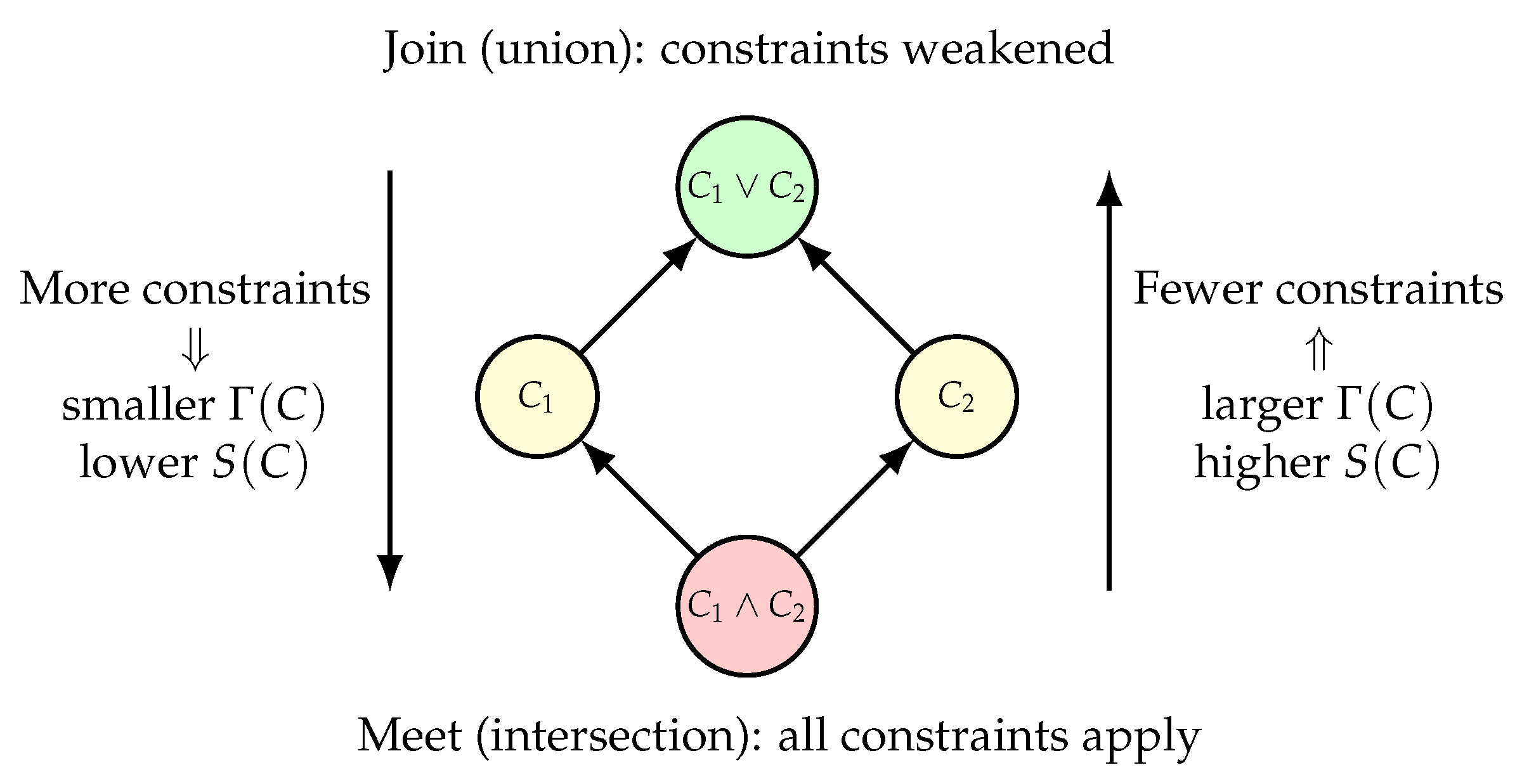
Figure A1 is a schematic illustration of a lattice structure of global constraints.
Figure A1.
Lattice structure of global constraint sets. The set of all constraint sets forms a partially ordered lattice with order relation meaning that contains fewer (weaker) constraints than C. The meet represents the combined constraint set (tighter constraints), while the join represents the weakened set retaining only the constraints common to both. Moving upward in the lattice corresponds to constraint decay, enlargement of the admissible microstate region , and an increase in the constraint–volume entropy .
Appendix B. Integrable Systems and Their Constraint Structure
Integrable systems play a distinguished role in the constraint–volume framework because they saturate the equality case of the Constraint Monotonicity Theorem. They possess extensive families of exactly conserved quantities, so the constraint set is time-independent and the entropy remains constant. Classical integrability is developed in standard references such as [53], and quantum integrability together with generalized Gibbs ensembles (GGE) is extensively reviewed in [28]. This appendix summarizes both cases in the language of constraint sets.
Appendix B.1. Classical Hamiltonian Integrability
Consider a classical Hamiltonian system with n degrees of freedom and canonical coordinates . The system is Liouville integrable if there exist n independent, globally defined integrals of motion
satisfying:
- (1)
- conservation under the flow:
- (2)
- mutual involution:
- (3)
- functional independence of the almost everywhere.
This is the standard Liouville–Arnold definition [53].
The conserved quantities define the constraint set
with admissible microstates
By the Liouville–Arnold theorem [53], each connected component of is diffeomorphic to an n-torus on which the motion is quasi-periodic. Under Hamiltonian time evolution,
so the admissible set and its volume are exactly preserved:
Thus classical integrable systems lie precisely on the entropy-preserving boundary of the structural Second Law.
Appendix B.2. Quantum Integrability and Conserved Operators
Quantum integrability has several definitions [58,59]. For lattice many-body systems, the most relevant characterization is the existence of an extensive family of mutually commuting conserved operators.
Let H act on a Hilbert space . A quantum system is integrable if there exists a family
such that:
- (1)
- (conservation),
- (2)
- (mutual commutativity),
- (3)
- the set is extensive and strongly constrains the dynamics [58].
Fixing their values defines the constraint set
with admissible states
Under unitary evolution,
and conservation implies
Hence
and the entropy is constant:
Quantum integrable systems therefore preserve global constraints exactly and do not exhibit generic entropy production.
Appendix B.3. Generalized Gibbs Ensembles (GGE)
A major insight in quantum integrability is that post-quench steady states are described not by canonical ensembles but by generalized Gibbs ensembles (GGE) [28,45]:
where the multipliers enforce
In the constraint–volume language, the GGE is the state of maximal von Neumann entropy over the admissible region :
Local equilibration may occur toward the GGE, but the global constraint set remains fixed. Thus the constraint–volume entropy does not increase: any growth in subsystem entropy arises solely from partial tracing, not from constraint decay.
Appendix B.4. Integrability as a Boundary of the Second Law
Within the constraint–volume framework, classical and quantum integrable systems share the same structural features:
- a large constraint set C that is exactly preserved,
- an invariant admissible set ,
- and a time-independent entropy .
Hence they satisfy
Any perturbation breaking integrability—for example, adding non-commuting terms to the Hamiltonian—reduces the constraint set:
and initiates the generic entropy growth described in the main text.
Appendix B.5. Summary
Classical and quantum integrable systems possess large, exactly conserved sets of global constraints. In the constraint–volume framework, they represent precisely the entropy-preserving boundary of the structural Second Law: the constraint set is invariant, the admissible microstate-space volume is fixed, and the entropy remains constant. Integrability thus acquires a clear geometric interpretation as the limiting case separating generic entropy-increasing dynamics from exceptional, symmetry-protected behavior.
Appendix C. Connection to von Neumann Entropy
In this appendix we show that the von Neumann entropy arises naturally as a special case of the constraint–volume entropy introduced in the main text. The central observation is that fixing a reduced density matrix or a set of quantum expectation values imposes a family of global algebraic constraints on the full state. The von Neumann entropy then coincides, up to an affine normalization, with the logarithmic volume of the admissible set of global states compatible with those constraints. This perspective connects directly to geometric analyses of quantum state space [30,33] and induced measures on density matrices [29].
Appendix C.1. Quantum State Space and Invariant Measures
Let be a d-dimensional Hilbert space. The convex set of density matrices,
admits several natural unitarily invariant measures. Two are especially relevant:
Either choice provides a well-defined volume functional on measurable subsets of , making the constraint–volume entropy fully applicable in the quantum setting.
Appendix C.2. Constraint Sets Defined by Fixed Reduced States
Consider a bipartite Hilbert space
Fix a reduced state on subsystem A. This fixes the global constraint
and the corresponding admissible global states form the fiber
The associated constraint–volume entropy is
Our goal is to show that reproduces the von Neumann entropy
up to an affine transformation that depends only on .
Appendix C.3. Volume of Fibers and Unitary Orbits
Let
be the spectral decomposition. All purifications of on form a single orbit under acting on subsystem B [60,61].
Moreover, the distribution of eigenvalues arising from partial traces of Haar-random pure states is described by induced Wishart ensembles [29]. These results imply that the measure of the fiber is determined solely by the eigenvalue spectrum .
Lemma A8
(Fiber-volume scaling). For fixed subsystem dimensions with , the volume of the constraint fiber satisfies
where the exponent depends on the choice of unitarily invariant measure (Hilbert–Schmidt, Bures, Haar–induced, etc.). The precise value of c does not affect the spectral functional form or the affine relation between the constraint–volume entropy and the von Neumann entropy; only the dependence on the eigenvalues is relevant for the comparison.
Proof
(Sketch). Using the induced-measure representation [29], density matrices with fixed reduced spectrum arise as partial traces of Haar-random purifications. The eigenvalue distribution of the reduced state is proportional to the monomial factor ; restricting attention to the fiber for fixed and integrating over the Haar orbit gives the stated dependence. □
Taking logarithms gives
Hence
Up to affine normalization, this has the same spectral dependence as the von Neumann entropy.
Appendix C.4. von Neumann Entropy as Constraint–Volume Entropy
Recall that
For fixed subsystem dimensions , the constraint–volume entropy satisfies
Thus the two quantities are related by an affine map:
Therefore the von Neumann entropy is precisely the spectral part of the constraint–volume entropy associated with fixing a reduced density matrix.
Appendix C.5. Interpretation
The structural interpretation is immediate:
The von Neumann entropy is (up to normalization) the logarithmic volume of the set of global states compatible with the reduced density matrix .
This provides a direct geometric meaning for quantum entropy:
- Fixing imposes global algebraic constraints.
- The admissible global states form the fiber .
- The volume of this fiber quantifies how many global states are compatible with .
- The von Neumann entropy is the corresponding logarithmic volume, up to a universal affine scaling.
Thus subsystem entropy, entanglement entropy, and the geometry of constraint fibers are unified under a single structural principle.
Appendix C.6. Summary
- Fixing a reduced density matrix defines a global constraint set on the full quantum state.
- The admissible states form a fiber whose volume depends only on the eigenvalues of .
- The logarithmic fiber-volume reproduces the von Neumann entropy up to an affine normalization.
- This gives a geometric and structural explanation for the universality of the von Neumann entropy in quantum theory.
Appendix D. Continuous Systems and Measure Issues
The definition of constraint–volume entropy,
is straightforward for finite-dimensional systems equipped with a finite reference measure. However, many physically important systems possess continuous or infinite-dimensional state spaces: classical fields, quantum fields, continuum fluids, or gravitational configurations. In such settings, naive configuration-space volumes are typically infinite or ill-defined, requiring careful measure-theoretic treatment [25]. This appendix summarizes standard techniques—regularization, renormalization, entropy densities, and Radon–Nikodym constructions— under which and the associated entropy remain well-defined and physically meaningful.
Appendix D.1. Sigma-Finite Measures and Relative Volumes
Let be a measure space representing a continuous phase space, configuration space, or field configuration manifold. Such measures are typically σ-finite rather than finite [25]. For a constraint set C, the admissible set may satisfy
rendering the absolute entropy formally undefined.
What is well-defined are:
- relative volumes between two constraint sets, and
- entropy differences.
Even if and diverge, the ratio
may exist and be independent of the chosen regularization. This parallels standard constructions in statistical field theory and quantum field theory, where only differences in free energies or entropies are meaningful and UV-finite [62].
Appendix D.2. Regularization of Configuration Spaces
For classical fields, fluids, and continuum systems, configuration space is infinite-dimensional. A standard approach introduces ultraviolet and infrared regulators:
- a lattice spacing a (UV cutoff),
- a finite spatial volume V (IR cutoff).
This yields a finite-dimensional configuration space equipped with a finite measure [63]. For a constraint set C, define the regulated admissible region and the finite volume
The continuum limit is analyzed via the scaling of
in precise analogy with thermodynamic and continuum limits in statistical mechanics and Euclidean QFT. If a finite limit exists (possibly after multiplicative or additive renormalization), then the entropy difference
is well-defined and physically meaningful.
Appendix D.3. Entropy Densities and Extensivity
For extended systems, absolute entropies diverge with spatial volume. The physically relevant object is the entropy density. Let be a region of linear size L and volume . Define
where is the admissible region restricted to .
Under standard assumptions of thermodynamic stability and subadditivity, one expects the extensivity relation
yielding an intensive entropy density
Entropy-density differences,
capture structural changes in constraint sets and coincide with thermodynamic entropy differences in macroscopic systems.
Appendix D.4. Relative Entropy and Radon–Nikodym Derivatives
In infinite-dimensional settings, it is often natural to consider weighted measures. If is absolutely continuous with respect to with Radon–Nikodym derivative , then
Define the weighted entropy
Differences of the form correspond to ratios of weighted volumes and include, as special cases, various notions of relative entropy. In quantum theory, this connects to Umegaki relative entropy [64,65] and more general modular-theoretic entropies in von Neumann algebras, which remain finite provided the support conditions are satisfied.
Appendix D.5. Field-Theoretic and Gravitational Examples
In field theory and quantum gravity, configuration-space volumes appear as functional integrals,
which require UV regularization and renormalization [62]. Constraints correspond to restricting the functional integral to configs satisfying boundary conditions, conserved charges, topological sectors, or geometric invariants. Entropy differences then become differences of regulated partition functions.
In gravitational thermodynamics, the Bekenstein–Hawking entropy is interpreted as the logarithmic volume of geometries with fixed horizon area, with divergences canceled by background subtraction or counterterms in the Euclidean path integral [35,66,67]. Within the constraint–volume framework, this corresponds to the entropy of a constrained configuration space of geometries.
Appendix D.6. Summary
For continuous and infinite-dimensional systems, the absolute volume is typically divergent. However, the structural content of constraint–volume entropy is fully preserved by focusing on:
- relative volumes between admissible sets,
- entropy differences and entropy densities,
- regulated and renormalized configuration-space measures.
Under standard regularization schemes—lattice discretization, momentum cutoffs, functional measure normalization—the constraint–volume framework remains mathematically well-defined and naturally aligned with statistical mechanics, quantum field theory, and gravitational thermodynamics.
Appendix E. Constraint Decay Timescales
The structural Second Law established in the main text is kinematic: it connects the weakening of global constraints to the monotonic growth of the constraint–volume entropy. To relate this structural principle to concrete physical relaxation phenomena, we now characterize the timescales over which different classes of constraints decay. These timescales connect the order-theoretic notion of constraint weakening to familiar dynamical quantities such as decoherence, scrambling, diffusion, mixing, and relaxation [11,32].
Appendix E.1. Constraint Decay and Dynamical Generators
Let X denote the system’s state space (classical or quantum). Time evolution is generated by a one-parameter group or semigroup , where is the dynamical generator:
Relevant examples include:
Given an initial constraint set , its time-evolved form is the pushforward:
Under generic local dynamics, weakens monotonically—expressed as —and approaches a limiting constraint set determined by exact conservation laws.
Appendix E.2. Constraint Decay Functions and Characteristic Times
Let be the long-time admissible set. Define the constraint decay function
For continuous or infinite-dimensional state spaces, the volumes in this ratio are understood to be computed either within a finite spatial region or with respect to a normalized reference measure, so that both numerator and denominator are finite and the ratio is well-defined. This quantity measures the fraction of asymptotically admissible microstates that already satisfy the constraints at time t.
Definition A9
(Constraint decay timescale). If is monotone with , the constraint decay timescale is defined implicitly by
for a fixed small (e.g. or ), in analogy with the familiar relaxation time in kinetic theory.
Different classes of constraints—internal coherence relations, spatial gradients, correlation structures, hydrodynamic fields—have their own distinct decay functions and characteristic timescales.
Appendix E.3. Internal Constraints: Decoherence and Scrambling Times
Internal quantum constraints (phase coherence, purity, stabilizer relations, entanglement structure) decay due to both the system Hamiltonian and environmental couplings. Two canonical timescales arise:
Appendix E.25.25.53. Decoherence time τ dec .
Constraints fixing coherence relations () degrade on timescales of order .
Appendix E.25.25.54. Scrambling time τ scr .
In chaotic many-body systems, local perturbations rapidly spread across the entire system, erasing fine-grained constraints. The scrambling time is controlled by the butterfly velocity or the maximal Lyapunov exponent [69,70]. It marks the timescale at which initially localized correlations have become effectively delocalized.
Thus internal constraint sets satisfy
Appendix E.4. External Constraints: Relaxation, Mixing, and Transport
External constraints (density profiles, geometric order, gradient structures, macroscopic flows) decay on timescales governed by continuum transport and chaotic dynamics:
Appendix E.26.26.55. Diffusive relaxation time.
For a conserved density satisfying , an inhomogeneity of characteristic length L relaxes on the timescale
a standard result from diffusion theory [71].
Appendix E.26.26.56. Hydrodynamic relaxation time.
Velocity gradients in fluids relax according to
where is the kinematic viscosity. Constraints fixing flow patterns or shear profiles degrade on this scale.
Appendix E.26.26.57. Mixing time.
In chaotic Hamiltonian systems or turbulent flows, mixing destroys coarse-grained spatial correlations at rates determined by Lyapunov exponents and Ruelle–Pollicott resonances [72]. Thus approaches on mixing timescales.
Appendix E.5. Entropy Production Rates and Decay Exponents
Define . When S is differentiable, its production rate is
Near equilibrium, constraint decay is typically exponential:
leading to
More generally, the decay exponents are governed by the spectral properties of the generator (Liouvillian, Lindbladian, Markov generator), paralleling relaxation theory and spectral-gap analyses in nonequilibrium statistical mechanics [73].
Appendix E.6. Summary
Constraint-decay timescales provide the operational bridge between the structural Second Law and empirically measured relaxation dynamics:
- Internal constraints decay on decoherence and scrambling timescales.
- External constraints relax on diffusive, hydrodynamic, and mixing timescales.
- Entropy production rates reflect the dominant decay exponents in the spectrum of the dynamical generator.
The structural Second Law remains purely kinematic: entropy increases whenever global constraints weaken. The timescales described here quantify how quickly this weakening occurs in realistic systems, linking the geometric theory of entropy to experimentally accessible relaxation phenomena.
Appendix F. Technical Proofs
This appendix provides the formal support for the structural results used in the main text. We establish the monotonicity of admissible regions under constraint weakening, derive the entropy monotonicity theorem, analyze the evolution of constraint sets under dynamical semigroups, and clarify the special role of integrable systems. Throughout, denotes a measurable state space with a -finite reference measure [74], and all constraint sets are measurable.
Appendix F.1. Monotonicity of Constraint Volumes
We begin with the order-theoretic structure underlying constraint sets.
Lemma A10
(Constraint Inclusion). Let and be constraint sets with . Then
Proof.
By definition,
If , then the intersection over contains all sets appearing in , hence . □
Lemma A11
(Volume Monotonicity). If , then
Proof.
By Lemma A10, . Monotonicity of measure yields the claim [74]. □
Theorem F.1 (Entropy Monotonicity).Theorem If , then
Proof.
Since , Lemma A11 directly implies the claim. □
This establishes the static form of the structural Second Law.
Appendix F.2. Constraint Sets Under Dynamical Evolution
Let be a measurable semigroup or group on X with generator (Hamiltonian vector field, Liouvillian, Lindbladian, or Markov generator) [73]. The evolution of constraint sets is defined by pullback:
To analyze their long-time behavior, we introduce the asymptotic constraint region.
Definition A12
(Asymptotic Constraint Set). A constraint set is asymptotic if
Lemma A13
(Existence of Asymptotic Region). If X is compact and is continuous, then
is nonempty, measurable, and invariant under .
Proof.
Nested intersections of nonempty closed subsets of a compact space are nonempty [75]. Measurability follows from the fact that closures of measurable sets are measurable. Invariance follows from
□
Theorem F.2 (Convergence to Asymptotic Region).Theorem If is mixing or ergodic with a unique invariant measure, then
Proof.
Thus non-integrable dynamics generically weaken constraints over time.
Appendix F.3. Integrability and Constraint Preservation
Integrable systems preserve large, non-decaying constraint sets [53].
Definition A14.
A system is integrable if it admits a family of invariants satisfying
whose joint level sets foliate X with positive measure.
Lemma A15
(Preservation of Integrable Constraints). If
then
Proof.
Since , x satisfies the constraints iff does. □
Theorem F.3 (Instability Under Perturbation).Theorem For small perturbations of an integrable system , integrable constraint sets persist only on a measure-zero subset of phase space, with typical constraint destruction occurring on timescales .
Proof.
By the Kolmogorov–Arnold–Moser (KAM) theorem [77], only invariant tori with Diophantine frequency vectors survive; their complement develops chaotic regions that break constraint preservation. □
Thus integrability corresponds precisely to the saturation case of the structural Second Law.
Appendix F.4. Entropy Production Under Reversible Dynamics
We now reconcile entropy growth with reversible microscopic evolution (Hamiltonian, unitary, or measure-preserving dynamics) [73,78].
Theorem F.4 (Irreversibility from Constraint Weakening).Theorem Let be invertible and measure-preserving. If constraints weaken,
then entropy increases:
Proof.
Reversibility implies for all measurable A. Constraint weakening enlarges the admissible region: . Thus the monotonicity of measure gives
and hence entropy increases. □
Thus entropy production stems from dynamical weakening of constraints, not from fundamental irreversibility in the microscopic laws.
Appendix F.5. Summary
This appendix establishes the formal backbone of the structural Second Law:
- Entropy is monotonic under constraint weakening.
- Admissible regions converge to asymptotic invariant sets under mixing or ergodic evolution.
- Integrable systems preserve constraint sets exactly but are unstable under generic perturbations.
- Entropy production is compatible with fully reversible microscopic dynamics.
These results provide rigorous support for the geometric, constraint-based formulation of entropy developed in the main text.
References
- L. Boltzmann, “On certain questions of the theory of gases,” Nature 51, 413 (1895).
- C. E. Shannon, “A mathematical theory of communication,” Bell Syst. Tech. J. 27, 379 (1948).
- D. N. Page, “Average entropy of a subsystem,” Phys. Rev. Lett. 71, 1291 (1993).
- J. D. Bekenstein, “Black holes and entropy,” Phys. Rev. D 7, 2333 (1973).
- S. W. Hawking, “Particle creation by black holes,” Commun. Math. Phys. 43, 199 (1975).
- G. J. Chaitin, “On the length of programs for computing finite binary sequences,” J. ACM 13, 547–569 (1966).
- L. Sklar, Physics and Chance, Cambridge University Press (1993).
- J. W. Gibbs, Elementary Principles in Statistical Mechanics, Yale University Press (1902).
- M. A. Nielsen and I. L. Chuang, Quantum Computation and Quantum Information, Cambridge University Press (2000).
- E. T. Jaynes, “Information theory and statistical mechanics,” Phys. Rev. 106, 620 (1957).
- W. H. Zurek, “Decoherence, einselection, and the quantum origins of the classical,” Rev. Mod. Phys. 75, 715–775 (2003).
- J. M. Deutsch, “Quantum statistical mechanics in a closed system,” Phys. Rev. A 43, 2046 (1991).
- M. Srednicki, “Chaos and quantum thermalization,” Phys. Rev. E 50, 888 (1994).
- M. V. Berry, “Regular and irregular semiclassical wavefunctions,” J. Phys. A 10, 2083 (1977).
- E. Ott, Chaos in Dynamical Systems, Cambridge University Press (2002).
- J. L. Lebowitz, “Boltzmann’s entropy and time’s arrow,” Physics Today 46(9), 32 (1993).
- R. Nandkishore and D. A. Huse, “Many-body localization,” Ann. Rev. Cond. Mat. Phys. 6, 15 (2015).
- J. Liouville, “Note on the variation of arbitrary constants,” J. Math. Pures Appl. 3, 342 (1838).
- L. Boltzmann, “On the relationship between the second law of the mechanical theory of heat and probability theory,” Sitzungsberichte der Kaiserlichen Akademie der Wissenschaften, 76, 373–435 (1877).
- J. von Neumann, Mathematische Grundlagen der Quantenmechanik, Springer (1932).
- L. D. Landau and E. M. Lifshitz, Fluid Mechanics, Pergamon Press (1959).
- In H. D. Zeh, The Physical Basis of the Direction of Time; Springer, 2007; H. D. Zeh, The Physical Basis of the Direction of Time, Springer (2007).
- E. H. Lieb and D. W. Robinson, “The finite group velocity of quantum spin systems,” Commun. Math. Phys. 28, 251–257 (1972).
- A. Einstein, “On the motion of small particles suspended in liquids,” Ann. Phys. 17, 549 (1905).
- In P. R. Halmos, Measure Theory; Springer, 1974; P. R. Halmos, Measure Theory, Springer (1974).
- E. Joos and H. D. Zeh, “The emergence of classical properties through environmental interaction,” Z. Phys. B 59, 223 (1985).
- M. Rigol et al., “Thermalization in isolated quantum systems,” Nature 452, 854 (2008).
- L. D’Alessio, Y. Kafri, A. Polkovnikov, and M. Rigol, “From quantum chaos to ETH,” Adv. Phys. 65, 239 (2016).
- K. Życzkowski and H.-J. Sommers, “Induced measures in mixed quantum states,” J. Phys. A 34, 7111 (2001).
- M. J. W. Hall, “Random quantum correlations and density operator distributions,” Phys. Lett. A 242, 123 (1998).
- A. Holevo, Statistical Structure of Quantum Theory, Springer (2001).
- H. P. Breuer and F. Petruccione, The Theory of Open Quantum Systems, Oxford University Press (2002).
- I. Bengtsson and K. Życzkowski, Geometry of Quantum States, 2nd ed., Cambridge University Press (2017).
- H.-J. Sommers and K. Życzkowski, “Bures volume of mixed quantum states,” J. Phys. A 36, 10083 (2003).
- R. M. Wald, “Black hole entropy is the Noether charge,” Phys. Rev. D 48, 3427 (1993).
- J. Liouville, “Note on the integration of differential equations of dynamics,” J. Math. Pures Appl. 20, 137 (1855).
- L. D. Faddeev and L. A. Takhtajan, Hamiltonian Methods in the Theory of Solitons, Springer (2007).
- V. I. Arnold, Mathematical Methods of Classical Mechanics, 2nd ed., Springer (1989).
- R. Nandkishore and D. A. Huse, “Many-body localization and thermalization in quantum statistical mechanics,” Ann. Rev. Condens. Matter Phys. 6, 15–38 (2015).
- R. Nandkishore and D. A. Huse, “Many-body localization and thermalization in quantum statistical mechanics,” Ann. Rev. Condens. Matter Phys. 6, 15–38 (2015).
- D. M. Basko, I. L. Aleiner, and B. L. Altshuler, “Metal–insulator transition in a weakly interacting many-electron system with localized states,” Ann. Phys. 321, 1126–1205 (2006).
- X.-G. Wen, Quantum Field Theory of Many-Body Systems, Oxford University Press (2016).
- D. Gottesman, Stabilizer Codes and Quantum Error Correction, Ph.D. thesis, Caltech (1997); arXiv:quant-ph/9705052.
- A. Y. Kitaev, “Fault-tolerant quantum computation by anyons,” Ann. Phys. 303, 2–30 (2003).
- M. Rigol et al., “Relaxation in a completely integrable system,” Phys. Rev. Lett. 98, 050405 (2007).
- H. Price, Time’s Arrow and Archimedes’ Point, Oxford University Press (1996).
- E. T. Jaynes, “Gibbs vs Boltzmann Entropies,” Am. J. Phys. 33, 391 (1965).
- J. Loschmidt, “Über den Zustand der Wärmegleichgewichts …,” Sitzungsberichte der Kaiserlichen Akademie der Wissenschaften 73, 128–142 (1876).
- J. L. Lebowitz, “Microscopic Reversibility and Macroscopic Behavior,” Physics Today 46(9), 32–38 (1993).
- R. Penrose, The Emperor’s New Mind, Oxford University Press (1989).
- E. L. Hahn, “Spin echoes,” Phys. Rev. 80, 580–594 (1950).
- L. Boltzmann, Lectures on Gas Theory, Cambridge Univ. Press (1896).
- V. I. Arnold, Mathematical Methods of Classical Mechanics, 2nd ed., Springer (1989).
- B. A. Davey and H. A. Priestley, Introduction to Lattices and Order, Cambridge University Press (2002).
- R. T. Rockafellar, Convex Analysis, Princeton University Press (1970).
- P. Billingsley, Convergence of Probability Measures, Wiley (1999).
- H. B. Callen, Thermodynamics and an Introduction to Thermostatistics, Wiley (1985).
- B. Sutherland, Beautiful Models, World Scientific (2004).
- V. E. Korepin et al., Quantum Inverse Scattering Method, Cambridge Univ. Press (1993).
- A. Uhlmann, “The transition probability in the state space of a *-algebra,” Rep. Math. Phys. 9, 273–279 (1976).
- R. Jozsa, “Fidelity for mixed quantum states,” J. Mod. Opt. 41, 2315–2323 (1994).
- J. Zinn-Justin, Quantum Field Theory and Critical Phenomena, Oxford Univ. Press (2002).
- K. G. Wilson and J. B. Kogut, “The renormalization group and the epsilon expansion,” Phys. Rep. 12, 75–199 (1974).
- H. Umegaki, “Conditional expectations in operator algebras,” Kodai Math. Sem. Rep. 14, 59 (1962).
- M. Ohya and D. Petz, Quantum Entropy and Its Use, Springer (1993).
- G. W. Gibbons and S. W. Hawking, “Action integrals and partition functions in quantum gravity,” Phys. Rev. D 15, 2752 (1977).
- A. Strominger and C. Vafa, “Microscopic origin of the Bekenstein–Hawking entropy,” Phys. Lett. B 379, 99 (1996).
- H. Risken, The Fokker–Planck Equation, 2nd ed., Springer (1989).
- Y. Sekino and L. Susskind, “Fast scramblers,” JHEP 10, 065 (2008).
- D. A. Roberts and D. Stanford, “Diagnosing chaos using four-point functions,” Phys. Rev. Lett. 115, 131603 (2015).
- J. Crank, The Mathematics of Diffusion, Oxford University Press (1975).
- L.-S. Young, “What are SRB measures?” Ann. Math. Studies 150 (2002).
- D. J. Evans and G. P. Morris, Statistical Mechanics of Nonequilibrium Liquids, Cambridge University Press (2008).
- V. I. Bogachev, Measure Theory, Vols. I–II, Springer (2007).
- J. R. Munkres, Topology, Prentice Hall (2000).
- P. Walters, An Introduction to Ergodic Theory, Springer (1982).
- J. Pöschel, “Integrability of Hamiltonian systems on Cantor sets,” Proc. ICM Vol. 2, 1531–1540 (2002).
- P. Gaspard, Chaos, Scattering, and Statistical Mechanics, Cambridge University Press (1998).
Figure 1.
Constraint geometry in state space. The full microstate space X is restricted by constraints , producing admissible regions . Their overlap is the set of microstates satisfying all constraints simultaneously. The smaller this region, the smaller the constraint–volume entropy .
Figure 1.
Constraint geometry in state space. The full microstate space X is restricted by constraints , producing admissible regions . Their overlap is the set of microstates satisfying all constraints simultaneously. The smaller this region, the smaller the constraint–volume entropy .
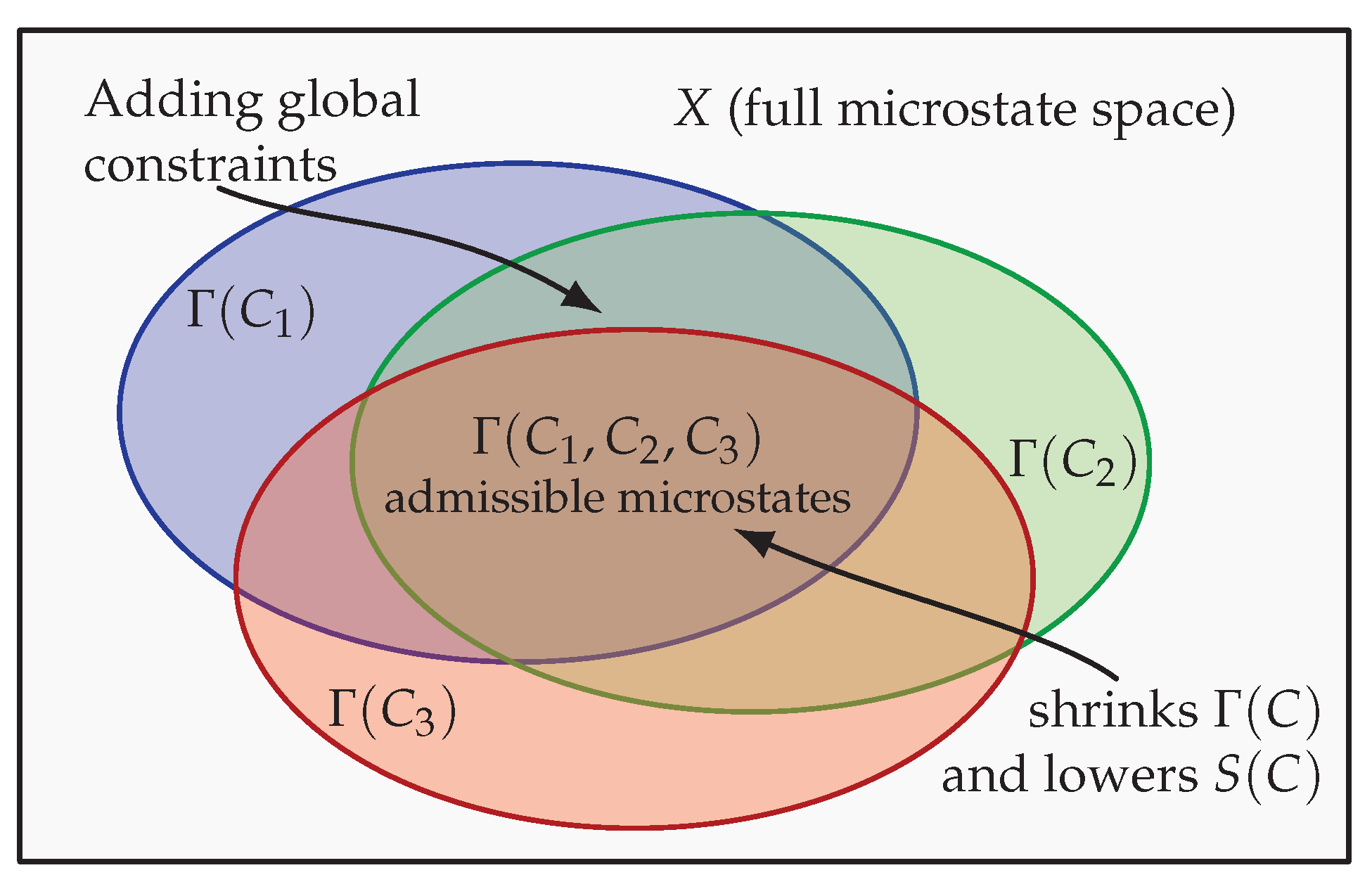
Figure 2.
Constraint decay under strictly local dynamics.Left: early universe or low-entropy states contain rich global non-separable constraints (entanglement, stabilizers, correlation structures). Middle: local interactions disrupt or decohere constraints but cannot create new global ones. Right: at late times the constraint network has largely decayed, increasing the number of compatible microstates and thus entropy. Locality ensures this decay is irreversible: global constraints can be destroyed but not created.
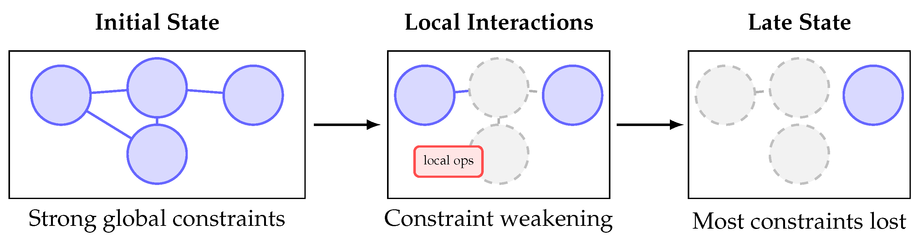
Figure 3.
Internal and external constraint decay. Left: Internal quantum constraints (coherence, entanglement, purity, stabilizers) represented as overlapping constraint circles. These constraints are fragile and rapidly destroyed by decoherence, scrambling, and quantum chaos. Right: External macroscopic constraints (density profiles, spatial correlations, hydrodynamic fields, gradients), represented as ellipses, decay slowly through diffusion, mixing, turbulence, and relaxation. Constraint decay enlarges the admissible region and increases entropy.
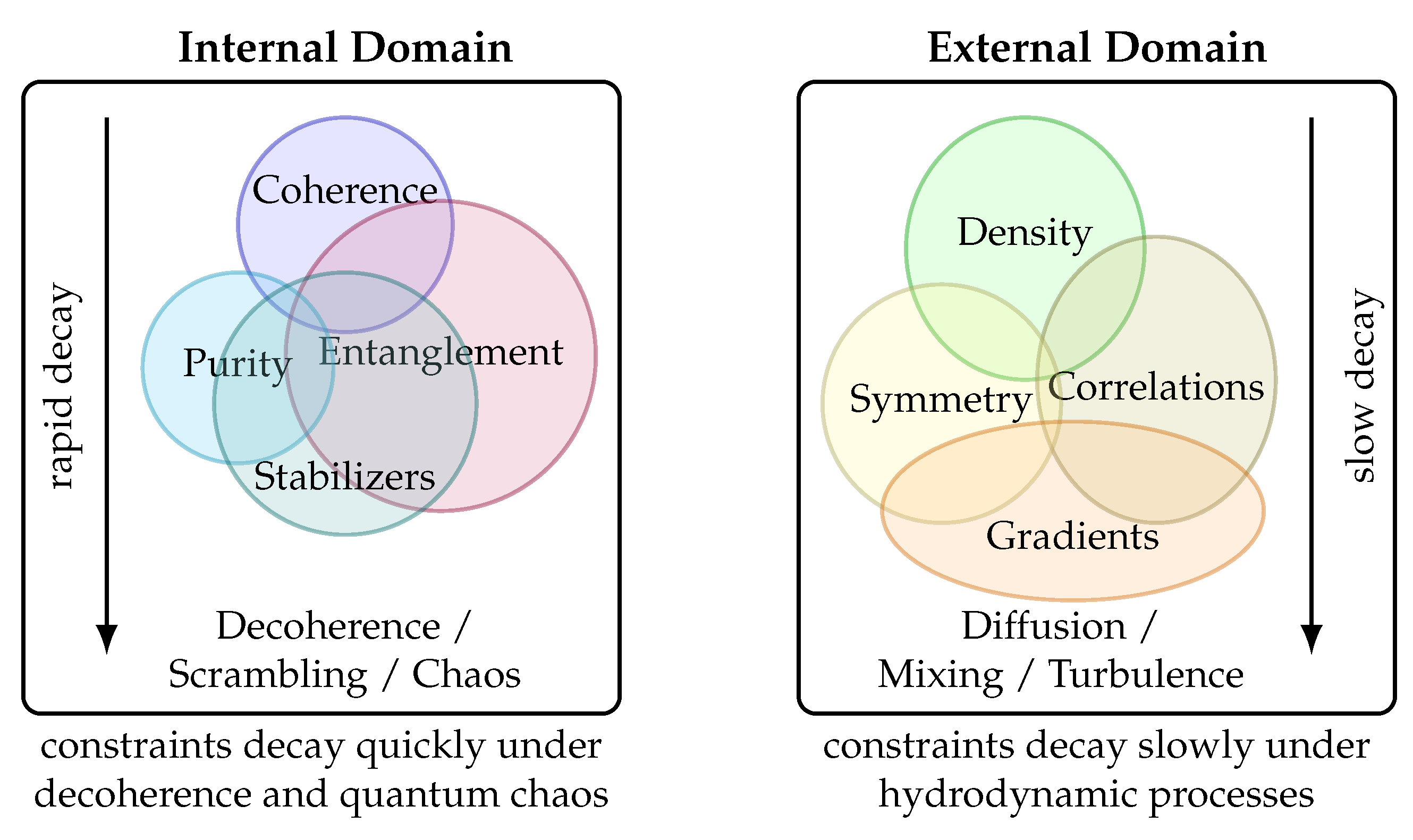
Figure 4.
Constraint decay enlarges the admissible microstate region. As global constraints weaken under generic local dynamics, the constraint sets satisfy . By monotonicity of admissible microstate sets, . The corresponding constraint–volume entropies obey , providing a geometric representation of the structural Second Law.
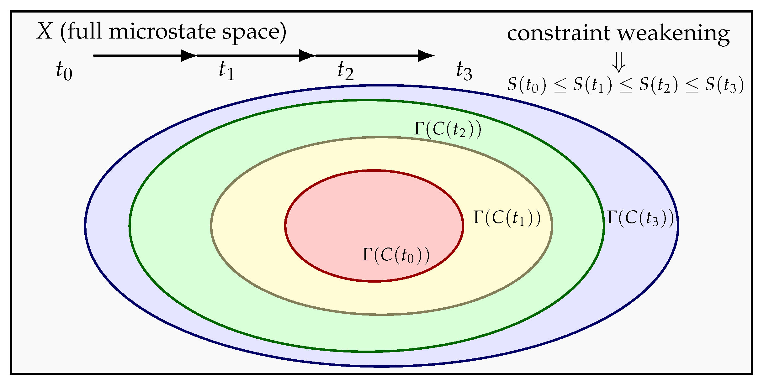
Figure 5.
Gas expansion as constraint loss. Initially the system satisfies a strong spatial constraint: all particles lie inside a subvolume . When the partition is removed, microscopic dynamics rapidly weaken this constraint, and the admissible microstate region expands to the full volume V. Because , the constraint–volume entropy increases by , reproducing the standard thermodynamic result without invoking coarse-graining.
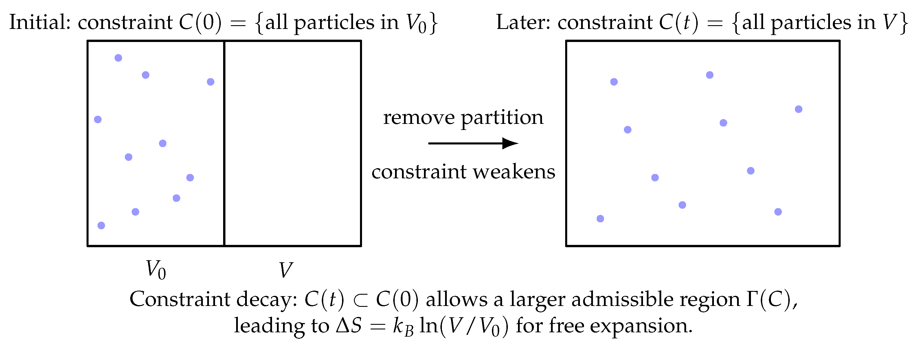
Figure 6.
Decoherence as decay of internal quantum constraints. Top-left: The initial Bell state is pure and has strong coherence constraints, visible as large off-diagonal terms in the density matrix. Centre: Interaction with an environment suppresses off-diagonal terms (loss of coherence), reduces purity, and destroys the entanglement constraint. Bottom-right: The final state is mixed and incoherent, with only diagonal components remaining. Constraint weakening enlarges the admissible quantum-state region and increases the constraint–volume entropy.
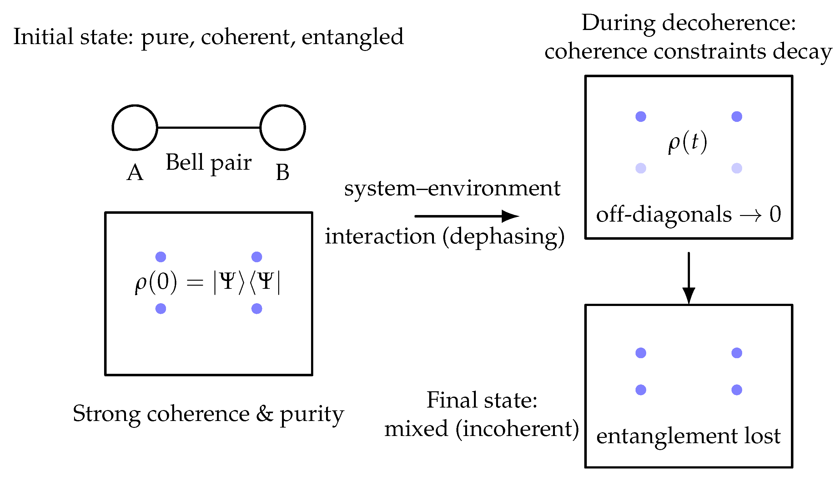
| 1 |
Disclaimer/Publisher’s Note: The statements, opinions and data contained in all publications are solely those of the individual author(s) and contributor(s) and not of MDPI and/or the editor(s). MDPI and/or the editor(s) disclaim responsibility for any injury to people or property resulting from any ideas, methods, instructions or products referred to in the content. |
© 2025 by the authors. Licensee MDPI, Basel, Switzerland. This article is an open access article distributed under the terms and conditions of the Creative Commons Attribution (CC BY) license (http://creativecommons.org/licenses/by/4.0/).
Copyright: This open access article is published under a Creative Commons CC BY 4.0 license, which permit the free download, distribution, and reuse, provided that the author and preprint are cited in any reuse.


