Time-Optimal Heliocentric Transfers With a Constant-Power, Variable-I_sp Engine

1. Introduction

While electric propulsion (EP) is traditionally valued for its propellant efficiency, future ambitious endeavors such as interplanetary logistics networks or rapid sample return missions will demand not just efficiency but speed [1,2,3]. For such missions, the design focus shifts from optimizing propellant mass to minimizing flight time, making the spacecraft’s power system the primary limiting factor [4]. Reducing transfer times from years to months propels interest in high-power propulsion systems, with gigawatt-class architectures representing a plausible long-term goal. Several pathways to this power scale are being explored, including advanced Nuclear Electric Propulsion (NEP) [5,6], next-generation deployable solar arrays [7], and beamed-energy concepts [8]. A common feature of these technologies is the ability to provide nearly constant power over long thrust arcs. This constant-power paradigm fundamentally alters the classic rocketry framework. Instead of the fixed exhaust velocity ($v_e$) of the Tsiolkovsky equation [9], the exhaust speed becomes a key control variable, allowing the engine to actively trade thrust for specific impulse. The Variable Specific Impulse Magnetoplasma Rocket (VASIMR) is an exemplary technology demonstrating this "constant-power throttling" over a wide operating range [10]. Such throttleability is compelling for the fast transfers that motivate our study, as recent optimization work confirms that varying the specific impulse during flight can significantly improve trip time [11]. In this paper, we develop the machinery to solve the time-optimal transfer problem in this high-power regime. We first derive an analytical solution for a 1D, gravity-free "brachistochrone" to build intuition. We then formulate the full planar Sun-field problem, derive two closed-form first integrals to simplify the dynamics, and present a robust numerical strategy to solve the resulting boundary-value problem. Our examples for a gigawatt-scale engine demonstrate Earth–Jupiter class transfers in a few months, frequently exploiting a solar Oberth maneuver.

2. Variable-$I_{sp}$ Rocket Model

Let $m\left(t\right)$ be the instantaneous mass ($m\ge m_{\mathrm{dry}}$) and $v_e\left(t\right)$ the exhaust speed. The propellant mass flow rate is the positive quantity ${\dot{m}}_f=-\dot{m}$. Neglecting plume inefficiencies, the thruster power P (constant) and thrust magnitude T are given by [12]:

$$P=\frac{1}{2}(-\dot{m})v_e^2,T=ma=(-\dot{m})v_e,$$

(1)

where a is the resulting thrust-induced acceleration magnitude. Eliminating $v_e$ gives a direct relationship between the mass flow rate and the vehicle’s acceleration:

$$\dot{m}=-{\displaystyle \frac{m^2{a}^2}{2P}}.$$

(2)

This equation forms the basis of our optimal control problem.

3. Exact Solution for the Free-Space Case $(\mu =0)$

With solar gravity absent ($\mu =0$), the translational degrees of freedom decouple. The problem simplifies to finding the minimum-time trajectory for a 1D drive from an initial state $(x,v)=(0,0)$ at $t=0$ to a final state $(x,v)=(L,0)$ at the final time $t_f$.

3.1. The Variational Method and the Hamiltonian

To find the optimal control history—in this case, the acceleration profile $a\left(t\right)$—we use the calculus of variations, specifically Pontryagin’s Maximum Principle (PMP) [13]. This powerful method converts the problem of minimizing a cost functional (like total time) into a problem of maximizing a new function, the Hamiltonian, at every point in time.

The Hamiltonian, $\mathcal{H}$, is constructed to package all essential information about the problem: the cost, the system dynamics, and the controls. The general formula is:

$$\mathcal{H}=L+{\lambda }^{\top }\mathbf{f}(\mathbf{x},\mathbf{u}),$$

(3)

where:

• L is the Lagrangian, or the instantaneous cost. For a minimum-time problem, the total cost is $J={\int }_0^{t_f}1dt$, so the instantaneous cost is simply $L=1$.
• $\mathbf{x}$ is the state vector, containing the variables that describe the system (e.g., position, velocity, mass).
• $\mathbf{u}$ is the control vector, containing the variables we can change to steer the system (e.g., acceleration).
• $\mathbf{f}(\mathbf{x},\mathbf{u})=\dot{\mathbf{x}}$ is the vector of state dynamics, describing how the system evolves.
• $\lambda$ is the costate vector, a set of auxiliary variables introduced by the PMP. Intuitively, each costate ${\lambda }_i\left(t\right)$ represents the sensitivity of the final cost to a small change in the state $x_i$ at time t. It is the "price" of that state variable.

3.2. Hamiltonian Construction for the Free-Space Case

We apply the principle from Section 3.1. First, we identify the components of the 1D problem:

• State vector:$\mathbf{x}={(x,v,m)}^{\top }$.
• Control variable:$u=a\left(t\right)$.
• State dynamics$\dot{\mathbf{x}}=\mathbf{f}(\mathbf{x},u)$:

  $$\begin{array}{cc}\hfill \dot{x}& =v,\hfill \end{array}$$

  (4)

  $$\begin{array}{cc}\hfill \dot{v}& =a,\hfill \end{array}$$

  (5)

  $$\begin{array}{cc}\hfill \dot{m}& =-{\displaystyle \frac{m^2{a}^2}{2P}}.\hfill \end{array}$$

  (6)
• Costate vector:$\lambda ={({\lambda }_x,{\lambda }_v,{\lambda }_m)}^{\top }$.

The term ${\lambda }^{\top }\dot{\mathbf{x}}$ in the Hamiltonian expands to:

$${\lambda }^{\top }\dot{\mathbf{x}}={\lambda }_x\dot{x}+{\lambda }_v\dot{v}+{\lambda }_m\dot{m}={\lambda }_{x}v+{\lambda }_{v}a-{\lambda }_m{\displaystyle \frac{m^2{a}^2}{2P}}.$$

Adding the Lagrangian $L=1$, we obtain the full Hamiltonian $\mathcal{H}$:

$$\mathcal{H}=1+{\lambda }_{x}v+{\lambda }_{v}a-{\lambda }_m{\displaystyle \frac{m^2{a}^2}{2P}}.$$

(7)

From this Hamiltonian, we derive the costate (adjoint) equations, given by $\dot{\lambda }=-\partial \mathcal{H}/\partial \mathbf{x}$:

$$\begin{array}{cc}\hfill {\dot{\lambda }}_x& =-{\displaystyle \frac{\partial \mathcal{H}}{\partial x}}=0,\hfill \end{array}$$

(8a)

$$\begin{array}{cc}\hfill {\dot{\lambda }}_v& =-{\displaystyle \frac{\partial \mathcal{H}}{\partial v}}=-{\lambda }_x,\hfill \end{array}$$

(8b)

$$\begin{array}{cc}\hfill {\dot{\lambda }}_m& =-{\displaystyle \frac{\partial \mathcal{H}}{\partial m}}={\lambda }_m{\displaystyle \frac{m{a}^2}{P}}.\hfill \end{array}$$

(8c)

3.3. Optimal Control and First Integrals

According to the PMP, the optimal control $a\left(t\right)$ must maximize the Hamiltonian at all times. We find it by setting $\partial \mathcal{H}/\partial a=0$:

$${\displaystyle \frac{\partial \mathcal{H}}{\partial a}}={\lambda }_v-{\lambda }_m{\displaystyle \frac{m^{2}a}{P}}=0\Rightarrow a\left(t\right)={\displaystyle \frac{P{\lambda }_v\left(t\right)}{{\lambda }_m\left(t\right)m^2\left(t\right)}}.$$

(9)

From the costate dynamics, we can extract two integrals of motion. First, (8a) directly implies:

$${\lambda }_x\left(t\right)=C_1=\mathrm{const}.$$

(10)

Substituting this into (8b) and integrating gives:

$${\lambda }_v\left(t\right)=-C_{1}t+C_2,$$

(11)

showing that the velocity costate is a linear function of time.

A second, less obvious, integral is found by examining the time derivative of the product ${\lambda }_m{m}^2$:

$$\begin{array}{cc}\hfill {\displaystyle \frac{d}{dt}}\left({\lambda }_m{m}^2\right)& ={\dot{\lambda }}_m{m}^2+{\lambda }_m\left(2m\dot{m}\right)\hfill \\ \hfill & =\left({\lambda }_m{\displaystyle \frac{m{a}^2}{P}}\right)m^2+{\lambda }_m\left(2m\left(-{\displaystyle \frac{m^2{a}^2}{2P}}\right)\right)\hfill \\ \hfill & ={\displaystyle \frac{{\lambda }_m{m}^3{a}^2}{P}}-{\displaystyle \frac{{\lambda }_m{m}^3{a}^2}{P}}=0.\hfill \end{array}$$

(12)

Thus, the product ${\lambda }_m\left(t\right)m^2\left(t\right)$ is constant throughout the trajectory:

$${\lambda }_m\left(t\right)m^2\left(t\right)=C_m=\mathrm{const}.$$

(13)

Substituting these integrals into the control law (9), we discover that the optimal acceleration profile must be linear in time:

$$a\left(t\right)={\displaystyle \frac{P}{C_m}}(-C_{1}t+C_2)=K_{1}t+K_0,$$

(14)

where $K_1=-P{C}_1/C_m$ and $K_0=P{C}_2/C_m$ are constants.

3.4. Deriving the Trajectory

We now determine the constants $K_1$ and $K_0$ by applying the boundary conditions. Let the final time be $t_f$. First, we integrate $a\left(t\right)$ to find the velocity $v\left(t\right)$:

$$v\left(t\right)={\int }_0^{t}a\left(\tau \right)d\tau +v\left(0\right)=\frac{1}{2}{K}_1{t}^2+K_{0}t.$$

(15)

Applying the final velocity condition $v\left(t_f\right)=0$:

$$\frac{1}{2}{K}_1{t}_f^2+K_0{t}_f=0\Rightarrow K_0=-\frac{1}{2}{K}_1{t}_f.$$

(16)

Substituting this back into $a\left(t\right)$ reveals its symmetric nature, a characteristic feature of such time-optimal "there-and-back" problems:

$$a\left(t\right)=K_{1}t-\frac{1}{2}{K}_1{t}_f=K_1(t-t_f/2).$$

(17)

Next, we integrate $v\left(t\right)$ to find the position $x\left(t\right)$:

$$x\left(t\right)={\int }_0^{t}v\left(\tau \right)d\tau +x\left(0\right)=\frac{1}{6}{K}_1{t}^3+\frac{1}{2}{K}_0{t}^2.$$

(18)

Applying the final position condition $x\left(t_f\right)=L$:

$$L=\frac{1}{6}{K}_1{t}_f^3+\frac{1}{2}{K}_0{t}_f^2.$$

(19)

Substituting $K_0=-{\displaystyle \frac{1}{2}}{K}_1{t}_f$ into the equation for L allows us to solve for $K_1$:

$$\begin{array}{cc}\hfill L& =\frac{1}{6}{K}_1{t}_f^3+\frac{1}{2}(-\frac{1}{2}{K}_1{t}_f)t_f^2\hfill \\ \hfill & =(\frac{1}{6}-\frac{1}{4})K_1{t}_f^3=-\frac{1}{12}{K}_1{t}_f^3.\hfill \end{array}$$

(20)

This gives $K_1=-12L/t_f^3$. Consequently, $K_0=-{\displaystyle \frac{1}{2}}(-{\displaystyle \frac{12L}{t_f^3}})t_f=6L/t_f^2$. The optimal acceleration is therefore:

$$a\left(t\right)={\displaystyle \frac{12L}{t_f^3}}\left({\displaystyle \frac{t_f}{2}}-t\right).$$

(21)

This corresponds to an initial acceleration phase, followed by a symmetric braking phase, with $a\left(t\right)$ crossing zero at mid-time. $t=t_f/2$. By substituting the constants back and simplifying, we obtain the full trajectory:

$$\begin{array}{cc}\hfill v\left(t\right)& ={\displaystyle \frac{6Lt}{t_f^2}}\left(1-{\displaystyle \frac{t}{t_f}}\right),\hfill \end{array}$$

(22)

$$\begin{array}{cc}\hfill x\left(t\right)& =L\left[3{\left(\frac{t}{t_f}\right)}^2-2{\left(\frac{t}{t_f}\right)}^3\right],\hfill \end{array}$$

(23)

which describes a cubic-in-time “S-curve” path.

3.5. Mass Evolution and Minimum Time

The mass evolution is governed by the separable differential equation (6). Integrating gives:

$$\begin{array}{cc}\hfill {\int }_{m_i}^{m\left(t\right)}{\displaystyle \frac{dm}{m^2}}& =-{\int }_0^t{\displaystyle \frac{a{\left(\tau \right)}^2}{2P}}d\tau \hfill \\ \hfill \Rightarrow {\displaystyle \frac{1}{m_i}}-{\displaystyle \frac{1}{m\left(t\right)}}& =-{\displaystyle \frac{1}{2P}}{\int }_0^{t}a{\left(\tau \right)}^{2}d\tau .\hfill \end{array}$$

(24)

The integral of $a{\left(t\right)}^2$ is:

$$\begin{array}{cc}\hfill {\int }_0^{t}a{\left(\tau \right)}^{2}d\tau & ={\int }_0^t{\left({\displaystyle \frac{12L}{t_f^3}}\right)}^2{\left({\displaystyle \frac{t_f}{2}}-\tau \right)}^{2}d\tau \hfill \\ \hfill & ={\displaystyle \frac{144L^2}{t_f^6}}{\left[-{\displaystyle \frac{1}{3}}{\left({\displaystyle \frac{t_f}{2}}-\tau \right)}^3\right]}_0^t\hfill \\ \hfill & ={\displaystyle \frac{48L^2}{t_f^6}}\left({\displaystyle \frac{t_f^3}{8}}-{\left({\displaystyle \frac{t_f}{2}}-t\right)}^3\right).\hfill \end{array}$$

(25)

Defining

$$f\left(s\right)=4s^3-6s^2+3s,$$

(26)

the mass relation becomes:

$${\displaystyle \frac{1}{m\left(t\right)}}-{\displaystyle \frac{1}{m_i}}={\displaystyle \frac{6L^{2}f(t/t_f)}{P{t}_f^3}}.$$

(27)

The total propellant consumed is found by setting $t=t_f$ (or $s=1$). If the entire propellant reserve is used, we have $m\left(t_f\right)=m_{\mathrm{dry}}$, which defines the minimum possible flight-time for the given distance L and mass fraction:

$$\Delta \equiv {\displaystyle \frac{1}{m_{\mathrm{dry}}}}-{\displaystyle \frac{1}{m_i}}$$

(28)

calculated as

$$\Delta ={\displaystyle \frac{6L^{2}f\left(1\right)}{P{T}_{min}^3}}={\displaystyle \frac{6L^2}{P{T}_{min}^3}}.$$

(29)

Solving for $T_{min}$ yields the final result:

$$T_{min}={\left[{\displaystyle \frac{6L^2}{P\Delta }}\right]}^{1/3}.$$

(30)

4. Transfers with a Finite Exhaust-Speed Ceiling

The linear-in-time acceleration profile from Section 3 is feasible only if the engine can raise its exhaust speed indefinitely, because $v_e\left(t\right)=2P/\left(m\left(t\right)a\left(t\right)\right)$ diverges when $a\left(t\right)\to 0$ at mid-time. A realistic thruster, however, is limited to a maximum effective exhaust speed $v_{e,max}$. This path constraint forces the optimal trajectory to switch the engine off once the required $v_e$ reaches the ceiling, producing the well-known boost-coast-brake structure [3,14].

This section derives the explicit solution for this case by adapting the unlimited solution. We introduce a coast phase and scale the acceleration profile to satisfy all physical constraints. The problem reduces to solving a single nonlinear equation for the optimal duration of the coast phase.

4.1. Setup and Scaled Trajectory

The trajectory consists of a burn, a coast, and a symmetric braking burn. We define a dimensionless switch fraction $\xi \equiv t_c/t_f\in (0,\frac{1}{2})$, where $t_c$ is the time when the engine is first shut down and $t_f$ is the total transfer time.

We adapt the acceleration profile from the unlimited case, $a_{\infty }\left(t\right)$ from (21), by scaling it with a constant throttle factor k. The powered phases now run from $t=0$ to $t_c$ and symmetrically at the end. The three unknowns (k, $t_f$, and $\xi$) are determined by the three physical constraints: total distance, total propellant, and the exhaust speed ceiling. The derivation uses the recurring polynomial $f\left(\xi \right)$ defined in (26), which is positive for $0<\xi <\frac{1}{2}$.

4.2. Derivation via Constraint Matching

Since the Pontryagin conditions are preserved on the powered arcs, the scaled linear-in-time profile with an inserted coast is an admissible PMP candidate; enforcing the three global constraints selects the optimal member of this family.

1.

Distance Closure

The total distance traveled, L, is the sum of distances covered during the first burn, the coast, and the final brake. Integrating the velocity profile for the scaled acceleration over the three segments and setting the sum to L uniquely determines the throttle scale k as a function of $\xi$:

$$k={\displaystyle \frac{1}{2f\left(\xi \right)}}.$$

(31)

2.

Propellant Closure

The total change in the inverse of mass, $\Delta$, must be consumed over the two symmetric powered phases. Integrating the mass-flow equation (2) using the scaled acceleration $a\left(t\right)=k{a}_{\infty }\left(t\right)$ gives:

$$\Delta =2{\int }_0^{t_c}{\displaystyle \frac{a{\left(t\right)}^2}{2P}}dt={\displaystyle \frac{k^2}{P}}{\int }_0^{t_c}{a}_{\infty }{\left(t\right)}^{2}dt.$$

(32)

Solving this for the total time $t_f$ and substituting $k=1/\left(2f\right(\xi \left)\right)$ yields the flight time as a function of the switch fraction:

$$t_f\left(\xi \right)={\left[{\displaystyle \frac{3L^2}{P\Delta f\left(\xi \right)}}\right]}^{1/3}.$$

(33)

3.

Exhaust Speed Ceiling

The final constraint is that the exhaust speed must not exceed its ceiling, $v_e\left(t\right)\le v_{e,max}$. The critical point is at the switch-off time $t=t_c$, where acceleration is lowest and mass has decreased. We impose the limit exactly at this point: $v_e\left(t_c\right)=2P/\left(m_{c}a\left(t_c\right)\right)=v_{e,max}$. The mass at this point, $m_c$, is the harmonic mean of the initial and dry masses, $m_c=2m_i{m}_{\mathrm{dry}}/(m_i+m_{\mathrm{dry}})$, since half the propellant is consumed. Substituting the expressions for $a\left(t_c\right)$, k, and $t_f\left(\xi \right)$ into this ceiling condition gives a single nonlinear equation for the optimal switch fraction ${\xi }_{★}$:

$$\begin{array}{cc}\hfill F\left(\xi \right)& =0,\mathrm{where}\hfill \end{array}$$

(34)

$$\begin{array}{cc}\hfill F\left(\xi \right)& \equiv \left(\frac{1}{2}-\xi \right)v_{e,max}-{\displaystyle \frac{P^{1/3}{L}^{1/3}f{\left(\xi \right)}^{1/3}}{3^{1/3}{\Delta }^{2/3}{m}_c}}.\hfill \end{array}$$

(35)

The function $F\left(\xi \right)$ is strictly decreasing on $0<\xi <\frac{1}{2}$, so if a root exists, it is unique.

4.3. Final Solution and Limiting Cases

The optimal transfer is found by solving the scalar equation $F\left(\xi \right)=0$ for the root ${\xi }_{★}\in (0,1/2)$ using any robust 1-D method. This value is then used in (33) to find the minimum transfer time.

Detecting whether the ceiling is active

If $F\left(\frac{1}{2}\right)\ge 0$, the ceiling is never touched. The optimal strategy is to never coast, and the minimum time is given by the unlimited-engine benchmark (30). Otherwise, a unique root ${\xi }_{★}$ exists, and the ceiling constraint is active.

Limiting Cases

• Unlimited engine. As $v_{e,max}\to \infty$, the root of $F\left(\xi \right)=0$ migrates to $\xi \to \frac{1}{2}$. In this limit, $f\left(\xi \right)\to 1/2$ and the flight time (33) collapses to the cubic root benchmark (30), recovering the solution from Section 3.
• Vanishing ceiling. When $v_{e,max}$ approaches the minimum useful value, $F\left(\xi \right)$ forces $\xi \to 0^{+}$. The two powered legs degenerate into instantaneous impulses separated by a long ballistic cruise, as intuition demands.

5. Full Planar Sun-Field Model

We now reinstate solar gravity ($\mu =G{M}_{\odot }$) and adopt polar coordinates $\mathbf{x}=(r,\theta )$ in the ecliptic. The control is the planar thrust acceleration${\mathbf{a}}_T=(a_r,a_{\theta })$ produced by the variable-$I_{sp}$ engine. The state vector and its dynamics are:

$$\begin{array}{cc}\hfill \dot{r}& =v_r,\hfill \end{array}$$

(36a)

$$\begin{array}{cc}\hfill \dot{\theta }& ={\displaystyle \frac{v_{\theta }}{r}},\hfill \end{array}$$

(36b)

$$\begin{array}{cc}\hfill {\dot{v}}_r& ={\displaystyle \frac{v_{\theta }^2}{r}}-{\displaystyle \frac{\mu }{r^2}}+a_r,\hfill \end{array}$$

(36c)

$$\begin{array}{cc}\hfill {\dot{v}}_{\theta }& =-{\displaystyle \frac{v_r{v}_{\theta }}{r}}+a_{\theta },\hfill \end{array}$$

(36d)

$$\begin{array}{cc}\hfill \dot{m}& =-{\displaystyle \frac{m^2}{2P}}\left(a_r^2+a_{\theta }^2\right).\hfill \end{array}$$

(36e)

5.1. Pontryagin Maximum Principle (PMP)

We again apply the variational framework from Section 3.1. For this time-optimal problem, the performance index is ${\displaystyle J={\int }_0^{t_f}\mathrm{d}t}$, meaning the Lagrangian is $L=1$. The components for the Hamiltonian construction are now:

• State vector:$\mathbf{x}={(r,\theta ,v_r,v_{\theta },m)}^{\top }$.
• Control vector:$\mathbf{u}={\mathbf{a}}_T={(a_r,a_{\theta })}^{\top }$.
• Costate vector:$\lambda ={({\lambda }_r,{\lambda }_{\theta },{\lambda }_{v_r},{\lambda }_{v_{\theta }},{\lambda }_m)}^{\top }$.

The Hamiltonian, $\mathcal{H}=1+{\lambda }^{\top }\dot{\mathbf{x}}$, must be maximized by the optimal control at all times. The dot product term ${\lambda }^{\top }\dot{\mathbf{x}}$ is constructed by multiplying each costate by its corresponding state derivative from (36):

$$\begin{array}{cc}\hfill {\lambda }^{\top }\dot{\mathbf{x}}=& {\lambda }_r{v}_r+{\lambda }_{\theta }{\displaystyle \frac{v_{\theta }}{r}}+{\lambda }_{v_r}\left({\displaystyle \frac{v_{\theta }^2}{r}}-{\displaystyle \frac{\mu }{r^2}}+a_r\right)\hfill \\ \hfill & +{\lambda }_{v_{\theta }}\left(-{\displaystyle \frac{v_r{v}_{\theta }}{r}}+a_{\theta }\right)-{\lambda }_m{\displaystyle \frac{m^2}{2P}}(a_r^2+a_{\theta }^2).\hfill \end{array}$$

(37)

Adding the Lagrangian $L=1$ gives the complete Hamiltonian for the sun-field model. For a minimum-time problem, the PMP asserts that along an optimal trajectory:

1.

The state and costates evolve according to Hamilton’s canonical equations: $\dot{\mathbf{x}}=\partial \mathcal{H}/\partial \lambda$ and $\dot{\lambda }=-\partial \mathcal{H}/\partial \mathbf{x}$.

2.

The optimal control ${\mathbf{a}}_T\left(t\right)$ maximizes $\mathcal{H}$ point-wise.

3.

The Hamiltonian remains constant and equal to zero: $\mathcal{H}\equiv 0$.

5.2. Optimal Control Law

To find the control that maximizes $\mathcal{H}$, we set the partial derivatives of the Hamiltonian with respect to the control variables $(a_r,a_{\theta })$ to zero:

$$\begin{array}{cc}\hfill {\displaystyle \frac{\partial \mathcal{H}}{\partial a_r}}& ={\lambda }_{v_r}-{\lambda }_m{\displaystyle \frac{m^2}{P}}{a}_r=0,\hfill \end{array}$$

(38a)

$$\begin{array}{cc}\hfill {\displaystyle \frac{\partial \mathcal{H}}{\partial a_{\theta }}}& ={\lambda }_{v_{\theta }}-{\lambda }_m{\displaystyle \frac{m^2}{P}}{a}_{\theta }=0.\hfill \end{array}$$

(38b)

This yields the optimal thrust acceleration vector:

$${\mathbf{a}}_T=k\left(t\right){\lambda }_v,\mathrm{where}{\lambda }_v\equiv {({\lambda }_{v_r},{\lambda }_{v_{\theta }})}^{\top },$$

(39)

and the time-varying gain factor is defined as

$$k\left(t\right)\equiv {\displaystyle \frac{P}{{\lambda }_m\left(t\right)m^2\left(t\right)}}.$$

(40)

The optimal thrust direction is parallel to the velocity costate vector ${\lambda }_v$. We now show that the gain factor $k\left(t\right)$ is, in fact, a constant of motion. Recent adaptive algorithms for low-thrust trajectory design exploit similar primer-vector structures to generate high-quality initial guesses for complex transfers [2].

5.3. Costate Equations and First Integrals

The costate dynamics are found from ${\dot{\lambda }}_i=-\partial \mathcal{H}/\partial x_i$:

$$\begin{array}{cc}\hfill {\dot{\lambda }}_r& ={\displaystyle \frac{{\lambda }_{\theta }{v}_{\theta }}{r^2}}+{\displaystyle \frac{{\lambda }_{v_r}{v}_{\theta }^2}{r^2}}-2{\lambda }_{v_r}{\displaystyle \frac{\mu }{r^3}}-{\lambda }_{v_{\theta }}{\displaystyle \frac{v_r{v}_{\theta }}{r^2}},\hfill \end{array}$$

(41a)

$$\begin{array}{cc}\hfill {\dot{\lambda }}_{\theta }& =-{\displaystyle \frac{\partial \mathcal{H}}{\partial \theta }}=0,\hfill \end{array}$$

(41b)

$$\begin{array}{cc}\hfill {\dot{\lambda }}_{v_r}& =-{\lambda }_r+{\lambda }_{v_{\theta }}{\displaystyle \frac{v_{\theta }}{r}},\hfill \end{array}$$

(41c)

$$\begin{array}{cc}\hfill {\dot{\lambda }}_{v_{\theta }}& =-{\displaystyle \frac{{\lambda }_{\theta }}{r}}-2{\lambda }_{v_r}{\displaystyle \frac{v_{\theta }}{r}}+{\lambda }_{v_{\theta }}{\displaystyle \frac{v_r}{r}},\hfill \end{array}$$

(41d)

$$\begin{array}{cc}\hfill {\dot{\lambda }}_m& =-{\displaystyle \frac{\partial \mathcal{H}}{\partial m}}={\lambda }_m{\displaystyle \frac{m}{P}}\left(a_r^2+a_{\theta }^2\right).\hfill \end{array}$$

(41e)

From these dynamics, we extract two first integrals.

• Rotational Symmetry

Equation (41b) arises because the Hamiltonian is independent of the absolute angle $\theta$ (a cyclic coordinate). This gives our first integral:

$$\begin{array}{|c|}\hline {\lambda }_{\theta }\left(t\right)=C_{\theta }=\mathrm{const}\\ \hline\end{array}.$$

(42)

• Mass–Costate Relationship

We find a direct relationship between mass m and its costate ${\lambda }_m$ by examining their rates of change. Using the chain rule, we have ${\displaystyle \frac{\mathrm{d}{\lambda }_m}{\mathrm{d}m}}={\displaystyle \frac{{\dot{\lambda }}_m}{\dot{m}}}$. Substituting from (41e) and (36)e:

$${\displaystyle \frac{\mathrm{d}{\lambda }_m}{\mathrm{d}m}}={\displaystyle \frac{{\lambda }_m\frac{m}{P}\left(a_r^2+a_{\theta }^2\right)}{-\frac{m^2}{2P}\left(a_r^2+a_{\theta }^2\right)}}={\displaystyle \frac{{\lambda }_{m}m}{-m^2/2}}=-2{\displaystyle \frac{{\lambda }_m}{m}}.$$

This is a separable first-order ordinary differential equation:

$${\displaystyle \frac{\mathrm{d}{\lambda }_m}{{\lambda }_m}}=-2{\displaystyle \frac{\mathrm{d}m}{m}}.$$

Integrating both sides yields $ln\left({\lambda }_m\right)=-2ln\left(m\right)+\mathrm{const}$, which upon exponentiation gives our second, crucial integral of motion:

$$\begin{array}{|c|}\hline {\lambda }_m\left(t\right)m^2\left(t\right)=C=\mathrm{const}\\ \hline\end{array}.$$

(43)

This relation holds for the entire trajectory.

• Constant Thrust Gain

Substituting the integral from (43) back into the definition of the gain factor (40), we find that it is constant:

$$k\left(t\right)={\displaystyle \frac{P}{{\lambda }_m\left(t\right)m^2\left(t\right)}}={\displaystyle \frac{P}{C}}\equiv k_T=\mathrm{const}.$$

(44)

The optimal control law (39) therefore simplifies to:

$${\mathbf{a}}_T\left(t\right)=k_T{\lambda }_v\left(t\right).$$

(45)

The thrust magnitude is proportional to the norm of the velocity costates, $\parallel {\lambda }_v\parallel$, and the proportionality factor $k_T$ is a constant determined by the boundary conditions. The discovery of this constant gain is a key analytical result, as it significantly simplifies the nature of the optimal control.

This completes the analytical formulation. The problem is reduced to a boundary-value problem governed by the seven differential equations for the state $(r,\theta ,v_r,v_{\theta })$ and non-constant costates $({\lambda }_r,{\lambda }_{v_r},{\lambda }_{v_{\theta }})$, with the control given by (45). A shooting method must find the initial values of the four costates $({\lambda }_r\left(0\right),C_{\theta },{\lambda }_{v_r}\left(0\right),{\lambda }_{v_{\theta }}\left(0\right))$ and the thrust constant $k_T$ that satisfy the specified final conditions at the optimal final time $t_f$.

6. Numerical Procedure

Solving the two-point boundary-value problem requires a numerical approach. We employ a two-stage strategy that combines a global search to find an initial, feasible trajectory with a local refinement process that uses a continuation method to precisely reach the desired target [3,11].

6.1. Objective Function

The core of the numerical method is an objective function, J, which quantifies the quality of a given trajectory. This function is minimized to find the optimal set of initial costate parameters. It incorporates penalties for violating physical constraints and errors for missing the target state. The function has two distinct forms depending on the optimization stage.

6.1.1. Global Search Objective

In the initial search phase, the goal is to find any valid transfer to a stable circular orbit, without a specific target location. The objective function, $J_{\mathrm{global}}$, is formulated to reward reaching a circular velocity in the outer solar system while penalizing physically unrealistic outcomes:

$$J_{\mathrm{global}}=w_f{\mathcal{P}}_f+w_r{\mathcal{P}}_r+w_v{\mathcal{E}}_v^2.$$

(46)

The terms are defined as:

• ${\mathcal{P}}_f$: A fuel penalty that applies a large constant value if the final mass $m_f$ drops below the dry mass $m_{\mathrm{dry}}$, effectively creating a hard constraint against using more fuel than available.
• ${\mathcal{P}}_r$: A radial position penalty, $max{(0,r_{\min }-r_f)}^2$, which discourages solutions that fail to travel a minimum distance $r_{\min }$ (e.g., 1.5 AU) from the Sun.
• ${\mathcal{E}}_v$: The velocity mismatch error at the final state. It measures the Euclidean distance between the final velocity vector ${\mathbf{v}}_f=(v_{r,f},v_{\theta ,f})$ and the required velocity for a circular orbit at the final radius $r_f$, given by ${\mathbf{v}}_{\mathrm{circ}}=(0,\sqrt{\mu /r_f})$. The squared error is ${\mathcal{E}}_v^2=v_{r,f}^2+{(v_{\theta ,f}-\sqrt{\mu /r_f})}^2$.
• $w_f,w_r,w_v$: Positive weighting constants that balance the contribution of each term.

6.1.2. Local Refinement Objective

Once an initial solution is found, the objective function is switched to a targeted version, $J_{\mathrm{local}}$, to steer the trajectory to a precise destination $(r_{\mathrm{des}},{\theta }_{\mathrm{des}})$:

$$J_{\mathrm{local}}=w_f{\mathcal{P}}_f+w_v{\mathcal{E}}_v^2+w_r{(r_f-r_{\mathrm{des}})}^2+w_{\theta }{({\theta }_f-{\theta }_{\mathrm{des}})}^2.$$

(47)

Here, the radial penalty ${\mathcal{P}}_r$ is removed, and two new terms are added to penalize deviations from the desired final radius $r_{\mathrm{des}}$ and true anomaly ${\theta }_{\mathrm{des}}$.

6.2. Two-Stage Optimization Strategy

6.2.1. Stage 1: Global Search

An initial, admissible solution is found by minimizing the global objective function (46). For this task, we use the differential_evolution algorithm from the SciPy library [15]. This robust, population-based method is well-suited for exploring the wide parameter space of the initial costates without getting trapped in local minima, thereby finding a good starting point for the next stage.

6.2.2. Stage 2: Continuation and Local Refinement

Starting from the solution found in Stage 1, which ends at a point $(r^{★},{\theta }^{★})$, we use a continuation (or homotopy) method to incrementally approach the final desired target $(r_{\mathrm{des}},{\theta }_{\mathrm{des}})$ [16]. The procedure is as follows:

1.

Set an intermediate target partway between the current known solution’s endpoint and the final desired endpoint.

2.

Perform a local optimization by minimizing the targeted objective function (47) using Powell’s method [17] (derivative-free) as implemented in scipy.optimize.minimize. The initial guess for the optimizer is the set of parameters from the previous successfully converged solution.

3.

If the optimizer converges to a high-precision solution, the new solution is accepted. The intermediate target is then advanced closer to the final destination, and the process repeats.

4.

If the optimizer fails to converge, it indicates the step to the new target was too large. The intermediate target is then moved back, typically halving the distance between the last successful endpoint and the current target, and the optimization is re-attempted.

• This adaptive stepping ensures that the local optimizer is always given a problem that is a small perturbation from a known good solution, guaranteeing robust convergence across the entire solution space until the final target is reached.

All simulations, optimization procedures, and figures were generated using the accompanying open-source Python implementation [18]. The repository includes the complete solver, plotting scripts, and resulting graphs of trajectories, fuel and acceleration magnitudes.

7. Results

The numerical procedure was applied to compute minimum-time transfers from a 1 AU circular orbit (representing Earth) to various target circular orbits. The targets are defined by their final radius and true anomaly relative to the starting position. A 1 GW engine was assumed with an initial vehicle mass of 3000 tons and a dry mass of 1000 tons.

Figure 1 and Figure 2 show the relationship between flight time and the orbital geometry. The flight times exhibit a U-shaped dependence on the final true anomaly, with a clear minimum for transfers that are neither direct short-arcs nor long-arcs. Similar behavior has been reported in recent multi-objective studies of variable-$I_{sp}$ maneuvers [11].

Figure 3 and Figure 5 show example trajectories. A key feature of these optimal paths is the inclusion of an Oberth maneuver. To gain orbital energy efficiently, the spacecraft first thrusts to lower its periapsis, making a close pass of the Sun. It then applies its main acceleration burn at maximum velocity near the Sun, which is far more effective at increasing orbital energy than thrusting in a higher orbit [19]. This is visible in the plots as an initial dip towards the Sun and a corresponding peak in the acceleration magnitude.

Table 1 and Table 2 present the resulting transfer times in days for a grid of targets. As expected, transfers to more distant orbits take longer. The notation ’N/A’ indicates that the transfer was not achievable with the given propellant load. This typically happens because there is a fixed constraint that cannot be overcome by continuous change of the initial conditions. Figure 5 shows trajectory very close to such a barrier, with very extreme Oberth maneuver around the Sun that cannot be extended further.

Figure 1. Flight times in days versus final true anomaly at arrival.

Figure 1. Flight times in days versus final true anomaly at arrival.

Figure 2. Flight times in days versus initial true anomaly at departure.

Figure 2. Flight times in days versus initial true anomaly at departure.

Figure 3. Example trajectory from $r=1$ AU, $\theta =0^{\circ }$ to $r=5$ AU, $\theta =273.1^{\circ }$ in 207 days. The trajectory includes a solar flyby (Oberth maneuver) to gain energy, which is apparent from the acceleration peak around day 50.

Figure 3. Example trajectory from $r=1$ AU, $\theta =0^{\circ }$ to $r=5$ AU, $\theta =273.1^{\circ }$ in 207 days. The trajectory includes a solar flyby (Oberth maneuver) to gain energy, which is apparent from the acceleration peak around day 50.

Figure 4. Example trajectory from $r=1$ AU, $\theta =0^{\circ }$ to $r=1.5$ AU, $\theta =34.7^{\circ }$ in 44 days. The trajectory is a very close analogy to the trajectories without gravity, demonstrating clear acceleration-deceleration pattern that is almost fully symmetric.

Figure 4. Example trajectory from $r=1$ AU, $\theta =0^{\circ }$ to $r=1.5$ AU, $\theta =34.7^{\circ }$ in 44 days. The trajectory is a very close analogy to the trajectories without gravity, demonstrating clear acceleration-deceleration pattern that is almost fully symmetric.

Figure 5. An example of a more extreme Oberth maneuver for a transfer to Jupiter’s orbit. The trajectory is from $r=1$ AU, $\theta =0^{\circ }$ to $r=5.2$ AU, $\theta =385.2^{\circ }$ and lasts 214 days.

Figure 5. An example of a more extreme Oberth maneuver for a transfer to Jupiter’s orbit. The trajectory is from $r=1$ AU, $\theta =0^{\circ }$ to $r=5.2$ AU, $\theta =385.2^{\circ }$ and lasts 214 days.

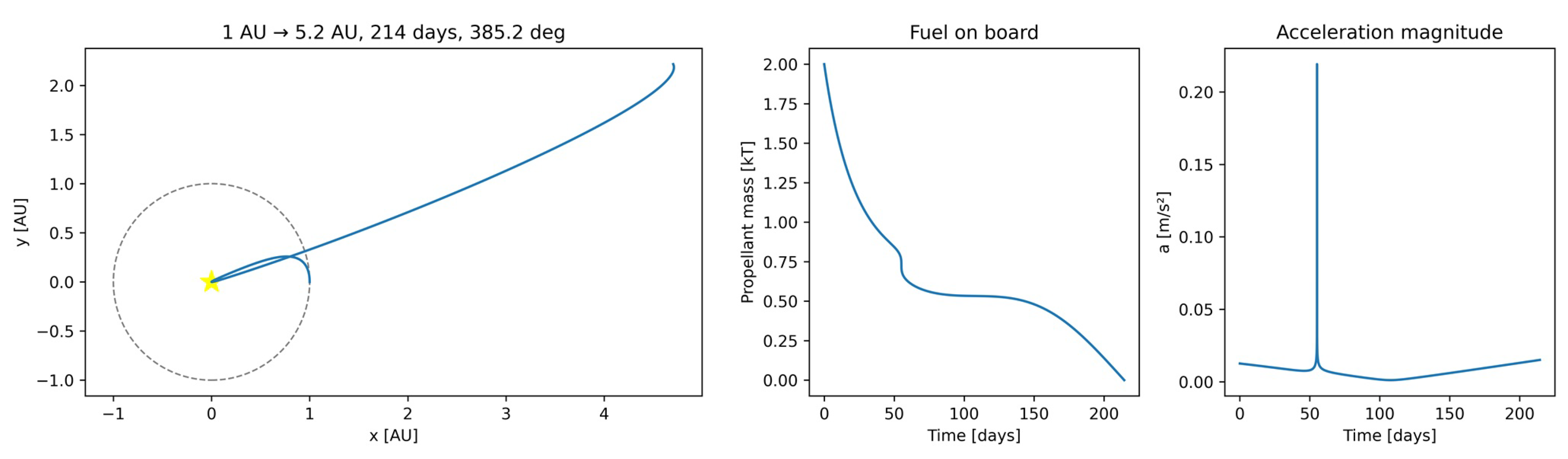
Table 3. Minimum transfer time (in days) to a circular orbit of 1 AU and final true anomaly (at rocket arrival).

True Anomaly	Origin Radius (AU)
(∘)	0.390	0.720	1.520	5.200	9.580	19.220	30.050
0	N/A	N/A	95.77	220.50	337.82	539.56	724.64
5	N/A	N/A	84.93	214.67	331.66	532.46	716.76
10	N/A	N/A	73.02	208.91	325.51	525.31	708.76
15	N/A	N/A	60.90	203.30	319.44	518.16	700.69
20	N/A	N/A	51.21	197.97	313.53	511.08	692.65
25	N/A	N/A	45.92	192.97	307.82	504.14	684.70
30	N/A	32.29	43.85	188.36	302.39	497.40	676.91
35	N/A	28.90	43.65	184.19	297.29	490.93	669.34
40	N/A	28.92	44.59	180.58	292.60	484.76	662.08
45	N/A	29.84	46.15	177.50	288.32	478.95	655.19
50	N/A	31.18	48.07	174.95	284.47	473.58	648.68
55	N/A	32.73	50.23	172.91	281.10	468.66	642.61
60	N/A	34.42	52.55	171.44	278.26	464.19	637.03
65	N/A	36.19	54.97	170.45	275.88	460.24	631.95
70	N/A	37.99	57.46	169.91	273.97	456.77	627.37
75	N/A	39.83	59.98	169.77	272.50	453.80	623.40
80	N/A	41.69	62.51	170.05	271.54	451.38	619.96
85	49.67	43.54	65.05	170.67	270.98	449.42	617.07
90	46.93	45.39	67.57	171.58	270.81	447.98	614.71
95	45.83	47.22	70.08	172.74	270.99	447.01	612.86
100	45.46	49.03	72.54	174.16	271.54	446.45	611.58
105	45.51	50.82	74.97	175.77	272.38	446.33	610.73
110	45.85	52.58	77.36	177.54	273.50	446.58	610.38
115	46.37	54.31	79.67	179.42	274.83	447.17	610.46
120	47.00	55.99	81.93	181.41	276.38	448.10	610.91
125	47.72	57.63	84.12	183.47	278.09	449.30	611.70
130	48.49	59.22	86.23	185.58	279.93	450.74	612.82
135	49.31	60.76	88.27	187.70	281.87	452.36	614.21
140	50.15	62.24	90.22	189.81	283.87	454.17	615.83
145	51.02	63.68	92.07	191.90	285.92	456.10	617.64
150	51.89	65.04	93.84	193.93	287.97	458.09	619.58
155	52.75	66.35	95.49	195.89	289.99	460.14	621.61
160	53.61	67.60	97.05	197.76	291.96	462.19	623.69
165	54.45	68.79	98.49	199.53	293.86	464.22	625.79
170	55.28	69.89	99.84	201.18	295.66	466.18	627.86
175	56.08	70.94	101.08	202.72	297.35	468.07	629.88
180	56.86	71.91	102.23	204.13	298.92	469.85	631.81
185	57.61	72.83	103.26	205.39	300.35	471.50	633.62
190	58.33	73.68	104.18	206.52	301.64	473.03	635.31
195	59.02	74.46	105.02	207.52	302.79	474.40	636.87
200	59.68	75.17	105.76	208.39	303.80	475.63	638.27
205	60.31	75.83	106.41	209.14	304.67	476.72	639.52
210	60.90	76.42	106.97	209.77	305.42	477.67	640.64
215	61.46	76.96	107.45	210.30	306.06	478.48	641.61
220	61.98	77.44	107.87	210.73	306.58	479.17	642.44
225	62.47	77.86	108.21	211.07	306.99	479.75	643.17
230	62.93	78.23	108.48	211.34	307.32	480.22	643.76
235	63.35	78.57	108.69	211.52	307.58	480.60	644.27
240	63.75	78.84	108.84	211.65	307.75	480.90	644.68
245	64.10	79.07	108.95	211.72	307.87	481.14	645.02
250	64.44	79.27	109.01	211.75	307.94	481.31	645.30
255	64.74	79.41	109.03	211.73	307.97	481.43	645.51
260	65.01	79.53	109.01	211.68	307.96	481.51	645.68
265	65.26	79.62	108.97	211.61	307.92	481.57	645.82
270	65.49	79.66	108.88	211.51	307.87	481.60	645.93
275	65.69	79.68	108.78	211.39	N/A	481.61	646.03
280	65.86	79.68	108.66	211.26	N/A	481.62	646.12
285	66.02	79.65	108.52	211.14	N/A	481.62	646.21
290	66.16	79.61	108.36	211.00	N/A	481.63	646.31
295	66.27	79.54	108.21	210.88	N/A	481.66	646.43
(∘)	0.390	0.720	1.520	5.200	9.580	19.220	30.050
300	66.38	79.47	108.04	210.75	N/A	481.71	646.57
305	66.47	79.37	107.87	210.65	N/A	481.78	646.75
310	66.56	79.27	107.70	210.56	N/A	481.89	646.96
315	66.63	79.17	107.54	210.49	N/A	482.04	647.22
320	66.70	79.07	107.39	210.44	N/A	482.24	647.54
325	66.76	78.97	107.25	210.43	N/A	482.48	647.93
330	66.83	78.89	107.13	210.45	N/A	482.79	648.38
335	66.90	78.80	107.03	210.51	N/A	483.16	648.91
340	66.99	78.74	106.97	210.60	N/A	483.61	649.55
345	67.08	78.70	106.94	210.75	N/A	484.14	650.27
350	67.19	78.70	106.94	210.96	N/A	484.76	651.11
355	67.32	78.73	107.00	211.22	N/A	485.47	652.06
360	67.48	78.82	107.10	211.54	N/A	486.28	653.13

Table 3. Minimum transfer time (in days) to a circular orbit of 1 AU and final true anomaly (at rocket arrival).

True Anomaly	Origin Radius (AU)
(∘)	0.390	0.720	1.520	5.200	9.580	19.220	30.050
0	N/A	N/A	95.77	220.50	337.82	539.56	724.64
5	N/A	N/A	84.93	214.67	331.66	532.46	716.76
10	N/A	N/A	73.02	208.91	325.51	525.31	708.76
15	N/A	N/A	60.90	203.30	319.44	518.16	700.69
20	N/A	N/A	51.21	197.97	313.53	511.08	692.65
25	N/A	N/A	45.92	192.97	307.82	504.14	684.70
30	N/A	32.29	43.85	188.36	302.39	497.40	676.91
35	N/A	28.90	43.65	184.19	297.29	490.93	669.34
40	N/A	28.92	44.59	180.58	292.60	484.76	662.08
45	N/A	29.84	46.15	177.50	288.32	478.95	655.19
50	N/A	31.18	48.07	174.95	284.47	473.58	648.68
55	N/A	32.73	50.23	172.91	281.10	468.66	642.61
60	N/A	34.42	52.55	171.44	278.26	464.19	637.03
65	N/A	36.19	54.97	170.45	275.88	460.24	631.95
70	N/A	37.99	57.46	169.91	273.97	456.77	627.37
75	N/A	39.83	59.98	169.77	272.50	453.80	623.40
80	N/A	41.69	62.51	170.05	271.54	451.38	619.96
85	49.67	43.54	65.05	170.67	270.98	449.42	617.07
90	46.93	45.39	67.57	171.58	270.81	447.98	614.71
95	45.83	47.22	70.08	172.74	270.99	447.01	612.86
100	45.46	49.03	72.54	174.16	271.54	446.45	611.58
105	45.51	50.82	74.97	175.77	272.38	446.33	610.73
110	45.85	52.58	77.36	177.54	273.50	446.58	610.38
115	46.37	54.31	79.67	179.42	274.83	447.17	610.46
120	47.00	55.99	81.93	181.41	276.38	448.10	610.91
125	47.72	57.63	84.12	183.47	278.09	449.30	611.70
130	48.49	59.22	86.23	185.58	279.93	450.74	612.82
135	49.31	60.76	88.27	187.70	281.87	452.36	614.21
140	50.15	62.24	90.22	189.81	283.87	454.17	615.83
145	51.02	63.68	92.07	191.90	285.92	456.10	617.64
150	51.89	65.04	93.84	193.93	287.97	458.09	619.58
155	52.75	66.35	95.49	195.89	289.99	460.14	621.61
160	53.61	67.60	97.05	197.76	291.96	462.19	623.69
165	54.45	68.79	98.49	199.53	293.86	464.22	625.79
170	55.28	69.89	99.84	201.18	295.66	466.18	627.86
175	56.08	70.94	101.08	202.72	297.35	468.07	629.88
180	56.86	71.91	102.23	204.13	298.92	469.85	631.81
185	57.61	72.83	103.26	205.39	300.35	471.50	633.62
190	58.33	73.68	104.18	206.52	301.64	473.03	635.31
195	59.02	74.46	105.02	207.52	302.79	474.40	636.87
200	59.68	75.17	105.76	208.39	303.80	475.63	638.27
205	60.31	75.83	106.41	209.14	304.67	476.72	639.52
210	60.90	76.42	106.97	209.77	305.42	477.67	640.64
215	61.46	76.96	107.45	210.30	306.06	478.48	641.61
220	61.98	77.44	107.87	210.73	306.58	479.17	642.44
225	62.47	77.86	108.21	211.07	306.99	479.75	643.17
230	62.93	78.23	108.48	211.34	307.32	480.22	643.76
235	63.35	78.57	108.69	211.52	307.58	480.60	644.27
240	63.75	78.84	108.84	211.65	307.75	480.90	644.68
245	64.10	79.07	108.95	211.72	307.87	481.14	645.02
250	64.44	79.27	109.01	211.75	307.94	481.31	645.30
255	64.74	79.41	109.03	211.73	307.97	481.43	645.51
260	65.01	79.53	109.01	211.68	307.96	481.51	645.68
265	65.26	79.62	108.97	211.61	307.92	481.57	645.82
270	65.49	79.66	108.88	211.51	307.87	481.60	645.93
275	65.69	79.68	108.78	211.39	N/A	481.61	646.03
280	65.86	79.68	108.66	211.26	N/A	481.62	646.12
285	66.02	79.65	108.52	211.14	N/A	481.62	646.21
290	66.16	79.61	108.36	211.00	N/A	481.63	646.31
295	66.27	79.54	108.21	210.88	N/A	481.66	646.43
(∘)	0.390	0.720	1.520	5.200	9.580	19.220	30.050
300	66.38	79.47	108.04	210.75	N/A	481.71	646.57
305	66.47	79.37	107.87	210.65	N/A	481.78	646.75
310	66.56	79.27	107.70	210.56	N/A	481.89	646.96
315	66.63	79.17	107.54	210.49	N/A	482.04	647.22
320	66.70	79.07	107.39	210.44	N/A	482.24	647.54
325	66.76	78.97	107.25	210.43	N/A	482.48	647.93
330	66.83	78.89	107.13	210.45	N/A	482.79	648.38
335	66.90	78.80	107.03	210.51	N/A	483.16	648.91
340	66.99	78.74	106.97	210.60	N/A	483.61	649.55
345	67.08	78.70	106.94	210.75	N/A	484.14	650.27
350	67.19	78.70	106.94	210.96	N/A	484.76	651.11
355	67.32	78.73	107.00	211.22	N/A	485.47	652.06
360	67.48	78.82	107.10	211.54	N/A	486.28	653.13

Table 4. Minimum transfer time (in days) to a circular orbit of 1 AU and initial true anomaly (at rocket departure).

True Anomaly	Origin Radius (AU)
(∘)	0.390	0.720	1.520	5.200	9.580	19.220	30.050
-100	46.94	N/A	137.22	281.20	401.02	604.64	789.45
-95	46.28	N/A	133.71	279.71	400.45	605.10	790.72
-90	45.79	N/A	130.04	277.91	399.53	605.19	791.59
-85	45.47	N/A	126.23	275.81	398.24	604.86	792.02
-80	45.48	N/A	122.29	273.35	396.55	604.09	791.99
-75	45.94	N/A	118.16	270.58	394.50	602.83	791.40
-70	47.06	N/A	113.88	267.49	392.03	601.11	790.28
-65	49.09	N/A	109.49	264.09	389.19	598.93	788.57
-60	51.87	N/A	104.93	260.40	385.96	596.20	786.30
-55	54.64	N/A	100.21	256.39	382.37	593.01	783.38
-50	56.91	N/A	95.40	252.12	378.37	589.32	779.89
-45	58.67	N/A	90.40	247.61	374.03	585.12	775.84
-40	60.08	42.22	85.27	242.85	369.36	580.46	771.21
-35	61.20	39.24	80.06	237.91	364.41	575.38	766.07
-30	62.11	36.39	74.72	232.81	359.17	569.87	760.34
-25	62.88	33.74	69.36	227.59	353.71	564.01	754.16
-20	63.51	31.37	64.05	222.28	348.05	557.81	747.56
-15	64.05	29.82	58.75	216.95	342.25	551.33	740.58
-10	64.50	28.85	53.84	211.66	336.37	544.62	733.26
-5	64.88	29.29	49.74	206.47	330.45	537.73	725.67
0	65.21	31.36	46.31	201.42	324.55	530.74	717.89
5	65.49	34.83	44.22	196.60	318.73	523.70	709.96
10	65.72	39.16	43.58	192.04	313.06	516.67	701.98
15	65.92	43.77	44.15	187.81	307.57	509.73	694.00
20	66.09	48.26	45.83	183.96	302.33	502.94	686.10
25	66.23	52.45	48.22	180.57	297.40	496.34	678.35
30	66.35	56.21	51.07	177.63	292.84	490.00	670.82
35	66.46	59.57	54.25	175.16	288.65	483.95	663.55
40	66.54	62.47	57.61	173.14	284.87	478.29	656.62
45	66.63	65.02	61.04	171.60	281.51	473.04	650.08
50	66.70	67.22	64.50	170.57	278.64	468.22	643.97
55	66.77	69.13	67.94	169.97	276.22	463.84	638.28
60	66.84	70.77	71.32	169.78	274.27	459.96	633.13
65	66.92	72.19	74.61	169.97	272.76	456.55	628.48
70	67.01	73.42	77.78	170.54	271.68	453.63	624.35
75	67.12	74.48	80.81	171.43	271.05	451.26	620.77
80	67.24	75.39	83.70	172.59	270.82	449.33	617.75
85	67.41	76.18	86.42	173.99	270.94	447.93	615.28
90	67.62	76.85	88.98	175.64	271.40	446.97	613.33
95	N/A	77.43	91.36	177.44	272.19	446.44	611.88
100	N/A	77.92	93.56	179.39	273.28	446.33	610.94
105	N/A	78.33	95.57	181.45	274.59	446.60	610.43
110	N/A	78.67	97.42	183.58	276.10	447.20	610.38
115	N/A	78.95	99.07	185.77	277.82	448.15	610.75
120	N/A	79.18	100.57	187.97	279.67	449.37	611.47
125	N/A	79.36	101.92	190.15	281.62	450.82	612.50
130	N/A	79.49	103.11	192.30	283.64	452.46	613.81
135	N/A	79.59	104.14	194.39	285.71	454.29	615.39
140	N/A	79.65	105.06	196.39	287.79	456.23	617.15
145	N/A	79.68	105.85	198.29	289.84	458.24	619.06
150	N/A	79.69	106.54	200.09	291.84	460.29	621.08
155	N/A	79.66	107.11	201.74	293.77	462.35	623.15
160	N/A	79.63	107.60	203.26	295.60	464.39	625.26
165	N/A	79.57	108.00	204.64	297.31	466.36	627.35
170	N/A	79.49	108.32	205.88	298.90	468.25	629.38
175	N/A	79.41	108.58	206.99	300.34	470.02	631.35
180	N/A	79.32	108.76	207.93	301.65	471.67	633.20
185	N/A	79.22	108.90	208.75	302.80	473.19	634.91
(∘)	0.390	0.720	1.520	5.200	9.580	19.220	30.050
190	N/A	79.12	108.98	209.46	303.82	474.54	636.50
195	N/A	79.02	109.02	210.05	304.69	475.76	637.95
200	N/A	78.93	109.03	210.52	305.45	476.84	639.25
205	N/A	78.85	108.99	210.92	306.08	477.77	640.40
210	N/A	78.77	108.93	211.22	306.59	478.57	641.40
215	N/A	78.72	108.84	211.44	307.01	479.25	642.26
220	N/A	78.70	108.73	211.59	307.34	479.81	643.01
225	N/A	78.71	108.60	211.70	307.59	480.28	643.64
230	N/A	78.76	108.46	211.74	307.76	480.64	644.17
235	N/A	78.87	108.30	211.74	307.88	480.93	644.60
240	N/A	79.06	108.15	211.71	307.94	481.17	644.95
245	N/A	N/A	107.97	211.64	307.97	481.33	645.24
250	N/A	N/A	107.81	211.56	307.96	481.44	645.47
255	N/A	N/A	107.65	211.45	307.92	481.52	645.64
260	N/A	N/A	107.49	211.33	307.87	481.57	645.79

Table 4. Minimum transfer time (in days) to a circular orbit of 1 AU and initial true anomaly (at rocket departure).

True Anomaly	Origin Radius (AU)
(∘)	0.390	0.720	1.520	5.200	9.580	19.220	30.050
-100	46.94	N/A	137.22	281.20	401.02	604.64	789.45
-95	46.28	N/A	133.71	279.71	400.45	605.10	790.72
-90	45.79	N/A	130.04	277.91	399.53	605.19	791.59
-85	45.47	N/A	126.23	275.81	398.24	604.86	792.02
-80	45.48	N/A	122.29	273.35	396.55	604.09	791.99
-75	45.94	N/A	118.16	270.58	394.50	602.83	791.40
-70	47.06	N/A	113.88	267.49	392.03	601.11	790.28
-65	49.09	N/A	109.49	264.09	389.19	598.93	788.57
-60	51.87	N/A	104.93	260.40	385.96	596.20	786.30
-55	54.64	N/A	100.21	256.39	382.37	593.01	783.38
-50	56.91	N/A	95.40	252.12	378.37	589.32	779.89
-45	58.67	N/A	90.40	247.61	374.03	585.12	775.84
-40	60.08	42.22	85.27	242.85	369.36	580.46	771.21
-35	61.20	39.24	80.06	237.91	364.41	575.38	766.07
-30	62.11	36.39	74.72	232.81	359.17	569.87	760.34
-25	62.88	33.74	69.36	227.59	353.71	564.01	754.16
-20	63.51	31.37	64.05	222.28	348.05	557.81	747.56
-15	64.05	29.82	58.75	216.95	342.25	551.33	740.58
-10	64.50	28.85	53.84	211.66	336.37	544.62	733.26
-5	64.88	29.29	49.74	206.47	330.45	537.73	725.67
0	65.21	31.36	46.31	201.42	324.55	530.74	717.89
5	65.49	34.83	44.22	196.60	318.73	523.70	709.96
10	65.72	39.16	43.58	192.04	313.06	516.67	701.98
15	65.92	43.77	44.15	187.81	307.57	509.73	694.00
20	66.09	48.26	45.83	183.96	302.33	502.94	686.10
25	66.23	52.45	48.22	180.57	297.40	496.34	678.35
30	66.35	56.21	51.07	177.63	292.84	490.00	670.82
35	66.46	59.57	54.25	175.16	288.65	483.95	663.55
40	66.54	62.47	57.61	173.14	284.87	478.29	656.62
45	66.63	65.02	61.04	171.60	281.51	473.04	650.08
50	66.70	67.22	64.50	170.57	278.64	468.22	643.97
55	66.77	69.13	67.94	169.97	276.22	463.84	638.28
60	66.84	70.77	71.32	169.78	274.27	459.96	633.13
65	66.92	72.19	74.61	169.97	272.76	456.55	628.48
70	67.01	73.42	77.78	170.54	271.68	453.63	624.35
75	67.12	74.48	80.81	171.43	271.05	451.26	620.77
80	67.24	75.39	83.70	172.59	270.82	449.33	617.75
85	67.41	76.18	86.42	173.99	270.94	447.93	615.28
90	67.62	76.85	88.98	175.64	271.40	446.97	613.33
95	N/A	77.43	91.36	177.44	272.19	446.44	611.88
100	N/A	77.92	93.56	179.39	273.28	446.33	610.94
105	N/A	78.33	95.57	181.45	274.59	446.60	610.43
110	N/A	78.67	97.42	183.58	276.10	447.20	610.38
115	N/A	78.95	99.07	185.77	277.82	448.15	610.75
120	N/A	79.18	100.57	187.97	279.67	449.37	611.47
125	N/A	79.36	101.92	190.15	281.62	450.82	612.50
130	N/A	79.49	103.11	192.30	283.64	452.46	613.81
135	N/A	79.59	104.14	194.39	285.71	454.29	615.39
140	N/A	79.65	105.06	196.39	287.79	456.23	617.15
145	N/A	79.68	105.85	198.29	289.84	458.24	619.06
150	N/A	79.69	106.54	200.09	291.84	460.29	621.08
155	N/A	79.66	107.11	201.74	293.77	462.35	623.15
160	N/A	79.63	107.60	203.26	295.60	464.39	625.26
165	N/A	79.57	108.00	204.64	297.31	466.36	627.35
170	N/A	79.49	108.32	205.88	298.90	468.25	629.38
175	N/A	79.41	108.58	206.99	300.34	470.02	631.35
180	N/A	79.32	108.76	207.93	301.65	471.67	633.20
185	N/A	79.22	108.90	208.75	302.80	473.19	634.91
(∘)	0.390	0.720	1.520	5.200	9.580	19.220	30.050
190	N/A	79.12	108.98	209.46	303.82	474.54	636.50
195	N/A	79.02	109.02	210.05	304.69	475.76	637.95
200	N/A	78.93	109.03	210.52	305.45	476.84	639.25
205	N/A	78.85	108.99	210.92	306.08	477.77	640.40
210	N/A	78.77	108.93	211.22	306.59	478.57	641.40
215	N/A	78.72	108.84	211.44	307.01	479.25	642.26
220	N/A	78.70	108.73	211.59	307.34	479.81	643.01
225	N/A	78.71	108.60	211.70	307.59	480.28	643.64
230	N/A	78.76	108.46	211.74	307.76	480.64	644.17
235	N/A	78.87	108.30	211.74	307.88	480.93	644.60
240	N/A	79.06	108.15	211.71	307.94	481.17	644.95
245	N/A	N/A	107.97	211.64	307.97	481.33	645.24
250	N/A	N/A	107.81	211.56	307.96	481.44	645.47
255	N/A	N/A	107.65	211.45	307.92	481.52	645.64
260	N/A	N/A	107.49	211.33	307.87	481.57	645.79

8. Conclusion

We combined analytic insight (two closed-form first integrals and a free-space benchmark solution) with a robust continuation strategy to solve the time-optimal transfer problem for a constant-power, variable-$I_{sp}$ engine. The method successfully generates high-performance trajectories, including those featuring Oberth maneuvers, for transfers out to the giant planets with a gigawatt-class engine. Recent developments in variable-$I_{sp}$ propulsion and adaptive low-thrust guidance algorithms [2,11] suggest that further improvements in mission performance are possible. Future work will extend this framework to three-dimensional rendezvous problems.

References

- Conway, B.A. (Ed.) Spacecraft Trajectory Optimization, Cambridge University Press: Cambridge, UK, 2010.
- Pino, B.P.; Howell, K.C. An energy-informed adaptive algorithm for low-thrust spacecraft cislunar trajectory design. In Proceedings of the AAS/AIAA Space Flight Mechanics Meeting, 2020; pp. AAS 20–579. [Google Scholar]
- Fogel, J.A.; Widner, M.; Williams, J.; Batcha, A. Multi-Impulse to Time Optimal Finite Burn Trajectory Conversion. Technical report, 2020; NASA Johnson Space Center. [Google Scholar]
- Mazouffre, S. Electric propulsion for satellites and spacecraft: established technologies and novel approaches. Plasma Sources Science and Technology 2016, 25, 033002. [Google Scholar] [CrossRef]
- Peakman, A.; Lindley, B. A review of nuclear electric fission space reactor technologies for achieving high-power output and operating with HALEU fuel. Progress in Nuclear Energy 2023, 163, 104815. [Google Scholar] [CrossRef]
- Scott, J.H. The Value Proposition of Multi-Megawatt Electric Power/Propulsion for the Human Exploration of Mars. In Proceedings of the International Astronautical Conference (IAC), 2019; p. number JSC-E-DAA-TN73357. [Google Scholar]
- Chang Díaz, F.R.; Carr, J.A.; Johnson, L.; Johnson, W.; Genta, G.; Maffione, P.F. Solar electric propulsion for human Mars missions. Acta Astronautica 2019, 160, 183–194. [Google Scholar] [CrossRef]
- Sheerin, T.F.; Petro, E.; Winters, K.; Lozano, P.; Lubin, P. Fast Solar System transportation with electric propulsion powered by directed energy. Acta Astronautica 2021, 179, 78–87. [Google Scholar] [CrossRef]
- Tsiolkovsky, K.E. Exploration of cosmic space by means of reaction devices, 1903. English translation; NASA TT F-243, 1965. [Google Scholar]
- Bering, E.A.; Longmier, B.W.; Ballenger, M.G.; Olsen, C.S.; Squire, J.P.; Chang Díaz, F.R. Performance studies of the VASIMR® VX-200. In Proceedings of the 49th AIAA Aerospace Sciences Meeting, Orlando, FL, 2011. [Google Scholar] [CrossRef]
- Di Pasquale, G.; Sanjurjo-Rivo, M.; Pérez Grande, D. A multi-objective variable-specific impulse maneuvers optimization methodology. Advances in Space Research 2024, 73, 20–30. [Google Scholar] [CrossRef]
- Sutton, G.P.; Biblarz, O. Rocket Propulsion Elements, 9th ed.; Wiley: New York, NY, 2017. [Google Scholar]
- Pontryagin, L.S.; Boltyanskii, V.G.; Gamkrelidze, R.V.; Mishchenko, E.F. The Mathematical Theory of Optimal Processes; Pergamon Press: Oxford, UK, 1962. [Google Scholar]
- Pontani, M. Optimal Space Trajectories with Multiple Coast Arcs Using Modified Equinoctial Elements. Journal of Optimization Theory and Applications 2021, 191, 545–574. [Google Scholar] [CrossRef]
- Storn, R.; Price, K. Differential evolution – a simple and efficient heuristic for global optimization over continuous spaces. Journal of Global Optimization 1997, 11, 341–359. [Google Scholar] [CrossRef]
- Allgower, E.L.; Georg, K. Numerical Continuation Methods: An Introduction; Springer: Berlin, Germany, 1990. [Google Scholar]
- Powell, M.J.D. An efficient method for finding the minimum of a function of several variables without calculating derivatives. The Computer Journal 1964, 7, 155–162. [Google Scholar] [CrossRef]
- Olšina, J. Time-Optimal Heliocentric Transfers With a Constant-Power, Variable-Isp Engine 2025. DOI:10.5281/zenodo.17521033. Code and data:. Available online: https://github.com/irigi/VariableISPRocketTrajectories. [CrossRef]
- Oberth, H. Die Rakete zu den Planetenr"aumen; R. Oldenbourg: Munich, Germany, 1923. English translation: The Rocket into Planetary Space. 1923. [Google Scholar]