
Submitted:
08 December 2025
Posted:
09 December 2025
You are already at the latest version
Abstract
The presented paper discusses and analyzes the methods for restoration of damaged stay rings and vanes of large Francis turbines. The focus is set on the crack damages that were also observed in stay vanes of Francis turbines in “Chaira” Pumped Hydro Energy Storage (PHES) plant, Hydro Unit 4 (HU4), where cracks occurred in all ten stay vanes. Additionally significant cavitation patches where noticed overall the front surface of the turbines stay vanes. Two approaches are examined in the study. The first approach for repairing adds material by welding over the damaged places, which are then polished. Although welding of damaged areas is a widespread method, some adverse effects are observed, mainly because of changes in the characteristics of the base metal and the impact of the high temperatures. The second approach is based on the removal of the damaged material till elimination of the cracks. Virtual models for computer simulation of both methods are prepared. These models are examined by structural mechanics and CFD analyses and compared. Final recommendations are proposed.
Keywords:
Francis turbines
; water flow investigation
; stay vanes restoration
; pumped hydro energy storage
1. Introduction
In Bulgaria, hydroelectric power plants are widespread, with the first one being built more than 120 years ago. Currently, hydroelectric power plants are particularly relevant for use in mixed role, i.e.,: Pumped Hydro-Electric Storage (PHES) plants. They are renewable energy sources, as they are either generators for electricity or powerful pumps, with the treated water being returned to reservoirs for reuse. One of the most powerful hydroelectric power plants in Europe is the PHES plant “Chaira”, build along the water cascade Belmeken – Sestrimo – Chaira. It is made up of four units with a total capacity of 864 MW as a generator and 788 MW in pumping mode. The integration of hydroelectric power plants into the country’s electricity transmission system is particularly relevant at a time when consumption in the system is strongly decreasing, and nuclear power plants and renewable energy sources continue to generate electricity.
Large Francis turbines, most often used in PHES plants, are subjected to high loads, high hydraulic pressures and accelerated wear of the working surfaces. These are most often the turbine blades, stay/guided vanes and covers. Rehabilitation and repair is mandatory during a certain time interval of operation. While the turbine blades and guided vanes are intended to be replaced, repair is difficult to implement for the stay vanes, covers and spiral casing. These are the elements that are subjected to intense wear, vibration, the occurrence of cracks, and cavitation causing surface destruction. Large Francis turbines in PHES plants are usually installed completely in concrete foundations and access for people and equipment to perform technological operations is highly difficult. Since this design constraint brings additional complexity and costs, many factors should be considered when deciding whether the stay vanes should be upgraded.
The company BBA Consultants published the article [1], which analyzes both the technical possibilities and the economic conditions for carrying out the repair of the stay vanes of large Francis turbines installed in a concrete foundation. In the paper two types of modifications of the damaged stay vanes are considered, i. e. re-profiling and adding extensions. Extensions could be made of steel or composites, depending on the needs and options offered by manufacturers performing the work. Each solution has both advantages and disadvantages. It is stated that the technical research necessary to make an informed decision must be detailed, thorough and carried out by qualified experts.
The modification of the stay vanes presents several technical challenges that require expert analysis. The potential increase in hydraulic efficiency associated with these modifications can justify the work from a financial point of view. However, the return on investment is usually higher for high-power units.
The aforementioned BBA Consultants company in its publication [2] presented the work carried out on the repair of the stay vanes, the spiral case and the covers a 125 MW Francis turbine in Turkey in 2021. Figure 1 and Figure 2 show the damages to the stay vanes and spiral casing after 10 years of operation. The stay vanes had lost thickness due to erosion. During a routine inspection, the surfaces had also been identified as being rough, resulting in a loss of efficiency and an increase in power consumption. The cause of roughness on the stay vanes was due to foreign matter (sand, silt, mud etc.) within the process [2]. The BBA Consultants recently completed a major turbine [1–3 repair project for a Hydroelectric Plant located in the Nueva Ecija province Central Luzon, The Philippines [3]. Two Francis turbines housed within the plant were suffering from corrosion, erosion due to cavitation in several key areas (Figure 3).
The experience gained in recent years, as well as the successfully implemented projects [1,2,3] for small and medium (175–200 MW) Francis turbines, do not give grounds to assume that the problems of repairing large PHES have been solved, especially for those around 800–1000 MW. The experience of the failure and repair of the PHES “Chaira” in Bulgaria [3,4,5], China [6], Canada [7] and many others prove the need for further research and experiments.
G.M. Shrum, BC Hydro largest facility in Canada [7] began operating in 1968 with ten turbine-generating units. Units 1 to 5 were installed in 1968 and 1969 with a capacity of 261 MW each. On March 2, 2008, the Unit 3 runner experienced a major failure. Except the runner many other components of the unit were damaged including stay and guided vanes. In Figure 4 shows guided vane damages uncovered after the runner failure. The skin plate of all 24 guided vanes had deep gouges on up to 75 percent of the metal surface. Cracks and surface damages of guided and stay vanes were repaired using welded plates and/or secured bolts. Heat treatment was applied to eliminate thermal stresses.
Large hydroelectric turbines are designed for many years of operation, due to the significant costs of design and production, environmental impact, their importance to the economy, difficulties in replacement and costly repairs. Resetting a large turbine to the original state or an upgrade with new hydraulic components is very costly or difficult to implement since, in case of a PHES plant, the unit is entirely placed in a concrete fundament. That is why the rehabilitation of the unit parts of a PHES plant is of vital importance, of which many papers in the scientific literature are published.
Bornard et al. [8] discussed the need and efficiency of the rehabilitation process for the large Francis hydro turbines. They proved that the gain in performance is significantly higher and could reach as much as 40% in output and up to 7% in efficiency, maximizing the return on investment of the rehabilitation project. In their paper they presented and analyzed the process of the existing water passages, identifying the hydraulic concerns and proposing adapted corrections to improve the performances.
Bornard et al. [8] discussed the need and efficiency of the rehabilitation process for the large Francis hydro turbines. They proved that the gain in performance is significantly higher and could reach as much as 40% in output and up to 7% in efficiency, maximizing the return on investment of the rehabilitation project. In their paper they presented and analyzed the process of the existing water passages, identifying the hydraulic concerns and proposing adapted corrections to improve the performances.
In [9] some aspects of the turbine hydraulic assessment and possible solutions to improve existing water passages in large Francis turbines are discussed. The aim of the authors is to increase the turbine capacity and revenues, eliminate cavitation erosion and the needs for repair, reduce the turbine instabilities and smooth unit regulation, and adapt the design to new operation conditions.
In [10] the experience of the company Alston in the hydro turbine rehabilitation field is discussed. Several specific cases encountered in the last few years in various hydro power stations of different countries are described. In the paper the stay vane profiles of a Francis turbine is modified in order to reduce their intrinsic losses, as well as to better suit with the guide vanes. Computational fluid dynamic calculations are applied for the stay vanes behavior improvement. In Figure 5 the effect of the optimization and improvement of the water flow and avoiding cavitation is shown.
Peng et al. [11] proposed a new methodology to reduce the vortex-induced vibration and improve the performance of the stay vane in a 200-MW Francis turbine. The optimization process was divided into two parts, i.e.,: diagnosis for the stay vane vibration based on field experiments and a finite element method for simulation and design. Finally, the optimized profile of a trailing edge was proposed for the stay vane. Verifications of the results using computational fluid dynamics simulations, structural analysis and fatigue analysis were performed to validate the optimized geometry.
In [12] the runner and the guided vanes of the Francis turbine were designed per the design head and flow rates available. Both the design and off-design conditions were simulated for the newly designed and existing turbines for comparison purposes. Cavitation performance of the new design was also determined. The authors claimed that the proposed methodology is applicable to any Francis type turbine and any PHES that needs rehabilitation.
Neto et al. [13] in there paper stated that the vortex-induced vibration in hydraulic turbines components (especially in stay vanes) is a well-known phenomenon it still remains challenging for operation and maintenance in the large hydro power plants. In their investigations of the stay vane cracks in a 250 MW Francis turbine in Brazil including an engineering study, structural and Computational Fluid Dynamics they analyzed the proper geometry modification of the stay vanes that could eliminate the periodic vortex induces vibrations. This modification was then implemented in the actual turbine stay vanes.
Zhang et al. [14] investigated the internal flow in a Francis Turbine for Comparing the Flow Noise of Different Operation Conditions. The study aimed to assist in the diagnosis of Francis turbine noise problems and their low-noise design. Umar et al. [15] experimentally investigated the flow performance of Francis turbines from a model to a prototype. They pretend that the methodology of their study can be generalized to other similar hydraulic turbines, especially prototype Francis turbines that lack experimental results.
According to the studies of publications in the scientific literature, established and reliable methods for restoration of the damaged areas of the stay vanes, the spiral casing and the upper and lower covers are material (steel) extension and re-profiling. The resent conclusions about the effectiveness of the methods for refurbishment these units of the Francis turbines was made in [1] and stated bellow.
Steel extensions are heavy to handle and require designing and installing a temporary monorail. They must also be adapted to existing and often irregular leading edge geometry. This may involve 3D laser measurements and tests with wooden mock-ups. Next, the heat generated by the welding process induces stresses in the stay vane and must be managed. Welding on a cast-iron stay vane is not recommended.
Re-profiling the stay vanes involves removing material from the leading or trailing edge, using either manual grinding or machining. Since stay vanes are typically under tension when the scroll case is watered, it’s necessary to validate that any local thinning will not compromise structural integrity. Care must also be taken to avoid exposing casting defects such as centerline shrinkage.
According to the authors [1] health and safety risks are present in all scenarios, particularly since the work is performed in a confined space where toxic emissions from welding gases or gouging can pose significant hazards.
In the present paper the methods for restoration of damaged stay rings and vanes of large Francis turbines are discussed. The focus is set on the crack damages that were also observed in stay vanes of Francis turbines in “Chaira” Pumped Hydro Energy Storage (PHES) plant, Hydro Unit 4 (HU4), where cracks occurred in all ten stay vanes. Additionally significant cavitation patches where noticed overall the front surface of the turbines stay vanes. Two approaches are examined in the study. The first approach for repairing adds material by welding over the damaged places, which are then polished. Although welding of damaged areas is a widespread method, some adverse effects are observed, mainly because of changes in the characteristics of the base metal and the impact of the high temperatures. The second approach is based on the removal of the damaged material till elimination of the cracks. Virtual models for computer simulation of both methods are prepared. These models are examined by structural mechanics and CFD analyses and compared. Final recommendations are proposed.
2. Materials and Methods
As presented in the section Introduction, the method of welding to restore the damaged sections of the stay vanes to their original shape leads to undesirable consequences. Such damages were observed to the turbines after the stay vanes repair of the PHES “Chaira”. Many studies [1,2,3,9,12,13] show that a good option is to clean the surface by removing the damaged metal. This leads to a change in the original shape of the stay vanes, which is assumed to lead to deterioration in the operational characteristics of the turbines. This section presents the methods for studying this influence, comparing them with the original operating characteristics at different loads in pumping and generator mode. The purpose of the study is to establish the influence of the geometry of the stay vanes on the power and torque of the working shaft.
Figure 6a shows the Francis turbine with the electric generator removed, showing the cover ring. Figure 6b shows the stay ring, stay and guided vanes that will be examined. Figure 7a shows a stay vane in its original shape, with the outlines of subsequent shape changes marked on it. Figure 7b shows a shape of the front face of the stay vane, corresponding to the initial removal of the damaged material. Figure 7c shows the final shape of the stay vane repaired.
The studies were carried out using modern methods of Computational Fluid Mechanics (CFD). In order to avoid errors due to differences in the computational mesh, the variants of the stay ring and vanes are represented as segments of their original shape. The computational mesh is the same for all three variants, and when the stay vanes are modified, the excess segments are transformed into fluid volumes.
The numerical model of the unit consists of 78,802,104 cells (Figure 8). A polyhedral mesh was used, which is particularly suitable for generating computational meshes for parts with complex geometry. In addition, polyhedral cells reduce the numerical error due to their higher quality compared to tetrahedral ones. The segmentation of the stay vanes leads to the creation of geometries with sharp edges at the separation points. This necessitates the use of a fine tetrahedral mesh, which is characterized by higher adaptability, but at the expense of lower quality. Figure 9 and Figure 10 show the generated meshes of the individual components. The type of computational mesh, the number of cells and their parameters are presented in Table 1 for each individual component. The mesh is densest around the contour of the stay vanes (Figure 10). A boundary mesh with 16 layers with the minimal height of the first layer of cells y = 200 µm was used. In Table 1 the inlet pressure Pin and outlet pressure Pout (the boundary conditions) for the generator and pump modes are presented.

Table 2.
The boundary conditions in generator and pump mode.
| Generator mode | Pump mode | ||
|---|---|---|---|
| Inlet pressure Pin (bar) | Outlet pressure Pout bar) | Inlet pressure Pin (bar) | Outlet mass flow rate Qout (kg/s) |
| 69.6 | 7 | 7 | 28 000 |
3. Results
3.1. Investigation of the Total Preasure of the Stay Vanes in Generator and Pump Modes
Figure 11 and Figure 12 the total pressure distribution around the modified area of the stay vanes in generator and pump mode respectively are shown. The numerical results are compared with the pressure distribution for the original form (Figure 11a) of the stay vanes (Variant 1). The data show that in turbine mode, the shortening of the stay vanes reduces the local pressures of the flow around the exit edge. The blue areas of the stay vane shape of Figure 11 (a) (Variant I) represent areas of lower pressure that can be potential sites for cavitation to develop. When the vanes are grind and polished, Figure 11b and Figure 11c (Variant II and III), these areas disappear, which leads to a reduction of the cavitation risk.
In the pump mode the opposite effect occurs. In Figure 12 (a) (Variant I) for the original shape it can be seen that the blue areas are replaced by red ones, which are an indicator of increased pressure. This shows that in pump mode for this red area of the stay vanes the pressure is higher which can lead to increase in hydraulic losses and mechanical torque. For the grinded stay vanes Variant II (Figure 12 b) the pressure is increased, while for the polished stay vanes Variant III (Figure 12 c) the pressure is lower and the red area almost vanishes.
3.2. Investigation of the Velosity Distribution Around the Stay and Guided Vanes in Generator and Pumpmodes
In this section the investigation of the velocity distribution in five planes perpendicular to the runner axis in generator mode are presented. In Figure 13 (a) the 3D shape of the stay and guided vanes, and the runner are shown. The planes (the lines in different colors) are located relative to the y-axis of the global coordinate system at positions -0.1 m, -0.05 m, 0 m, 0.05 m and 0.1 m. In Figure 13 (b) the plane Z – Y along the runner axes is presented. The aim is to assess the influence of the modified geometry of the stay vanes on the flow character through the flow section.
Further down, the investigations continue through a quantitative analysis of the velocity distribution around the stay vanes in generator mode (Figure 14, Figure 15, Figure 16, Figure 17, Figure 18, Figure 19, Figure 20, Figure 21, Figure 22 and Figure 23). The velocities are recorded along the contours of circles with diameters of 3650 mm and 4570 mm (Figure 13 a, b). This allows us to trace local accelerations, vortices and flow irregularities that affect the hydraulic losses and the torque of the runner. The largest differences in the flow characteristics are observed between Variant I (the initial form) and Variant III (the final form). The zones in which the flow changes occur are pointed out by red rectangles. This is the area between the trailing edge of the stay vanes and the trailing edge of the guided vanes. According to the flow picture, the shortening of the stay vanes leads to the formation of vortices. This effect becomes more visible after the addition of
the velocity formation of vortices. This effect becomes more visible after the addition of the velocity vectors (Figure 15, Figure 17, Figure 19, Figure 21 and Figure 23). The velocity distribution in five planes evenly spaced across the flow section shows that the velocity and flow character remain relatively uniform in height, without significant changes. This is typical of Francis turbines, since the flow in the flow section is largely axially symmetrical and the main changes in velocity and pressure are observed mainly in the flow direction.
The velocity distribution in pump mode is presented by the consequence of Figure 24, Figure 25, Figure 26, Figure 27, Figure 28, Figure 29, Figure 30, Figure 31, Figure 32 and Figure 33. The guided vanes create hydraulic resistance. Theoretically, this resistance can be reduced by increasing the maximum allowable opening angle of the guided vane. This change must be coordinated with the generator mode, since the increase in flow rate will affect the generator operation. The assessment of the velocity distribution around the stay vanes is more difficult due to the sharp change in the flow velocity after the guided vanes. For this purpose, velocity vectors (in black) have been added to track local accelerations and vortices. They clearly show that the flow hits the guided vanes after leaving the runner blades following their outline. This is a shock flow. After the flow overcomes the resistance of the guided vane, vortices are formed, clearly visible in the instantaneous flow pictures shown in the figures. For a complete description of the flow, a transient analysis is required, in which the instantaneous flow patterns are preserved for a certain time step. Since the purpose of the present analysis is to evaluate the influence of the geometry of the stay vanes, the available information is quite sufficient to show that the flow after the guided vanes is unstable in the pumping mode. Therefore, the pressure differences along the contour of the stay vanes are due not to the different shape of the columns, but to the current position of the formed vortices after the guided vanes. This shows that the influence of the shape of the stay vanes on the flow is insignificant compared to the influence of the non-uniform flow.
The hypothesis can be confirmed by quantitative analysis of the velocity distribution around the stay vanes. For this purpose, the velocity was recorded along the contours of circles with diameters of 3650 mm and 4570 mm (Figure 13 a, b), covering the area around the columns. The circles were projected onto the five planes perpendicular to the rotor axis. The results are presented in a polar coordinate system in Figure 34 and Figure 35 for generator mode and in Figure 36 and Figure 37 for pump mode. The characteristics resemble the shape of a star. The average velocities along the contour of each circle are summarized in Table 3, Table 4, Table 5 and Table 6. The data for the generator mode show that the flow is significantly more uniform.
The relative difference C [m/s] between the minimum and maximum average velocity is shown in Table 7, Table 8, Table 9 and Table 10. In pump mode (Figure 36 and Figure 37) the velocity field is noticeably more uneven. The contours are more distorted, and the imbalance between the minimum and maximum average values reaches 15.11% for the circles with a diameter of 3650 mm and 39.87% for 4570 mm. This clearly confirms the presence of instabilities and vortex formation after the guided vanes, which affect the local pressure and lead to increased hydraulic losses.
Figure 38 shows the process of convergence of the results (computation of the torques) in dependence on the iterative procedure of the numerical integration process. As can be seen, the characteristics of the three variants reach close points of convergence in both pumping and generator mode. The maximum relative difference is calculated between the variant with the smallest value and the variant with the largest value of the three, and in generator mode it is about 0.7%, and in pumping mode about 3.5%.
The results of the numerical analysis show that the geometry of the stay vanes has little effect on the energy characteristics of the unit. In generator mode, shortening the columns leads to a reduction in the low-pressure zones and a more uneven flow, without any significant differences in torque (below 1%). In this mode, the modification can be considered favorable from the point of view of cavitation risk.
In the pumping mode the process is more complex. There is a more uneven flow and larger fluctuations in the average velocity along the contour as the result of the strongly pronounced vortex formation after the guided vanes. This vortex flow dominates the influence of the geometry of the stay vanes, which makes it difficult to unambiguously assess the effect of their shortening. Therefore, it cannot be categorically concluded that the modification is unfavorable. Its influence is not dominant to the instabilities caused by the guided device.
4. Discussion
In summary, the analysis confirms the form of the guided vanes is decisive for the flow behavior, especially in pumping mode, while the shape of the stay vanes is of secondary importance.
Shortening the stay vanes does not impair the operation in generator mode, but on the contrary, it contributes to the reduction of low pressure zones and, accordingly, to the risk of cavitation. In pumping mode, the observed instabilities are mainly due to the vortex formation after the guided vanes, and not to the shape of the stay vanes, which means that the change in geometry does not have a decisive negative impact on the flow characteristics. In addition, the technical and economic argument remains fully valid, since shortening represents an easier and more cost-effective way to remove the compromised areas compared to their restoration by welding.
Author Contributions
Conceptualization, G.T. and K.K.; methodology, G.T., K.K. and Y.S.; software, B.Z.; validation, I.K. and Y.S.; formal analysis, G.T.; investigation, K.K. and B.Z.; resources, Y.S.; data curation, B.Z. and Y.S.; writing—original draft preparation, K.K.; writing—review and editing, G.T. and K.K.; visualization, Y.S., B.Z. and RI; supervision, I.K.; project administration, G.T. and I.K.; funding acquisition, I.K.; editing, consultation and review E.Z. All authors have read and agreed to the published version of the manuscript.
Data Availability Statement
The data presented in this study are available on request from the corresponding author. The data are not publicly available due to their relation to public funding specifics.
Conflicts of Interest
The authors declare no conflicts of interest.
References
- Payette, Félix-Antoine. Stay vanes refurbishment: factors to consider in decision makingр. 06 Aug 2024. Available online: https://www.bbaconsultants.com/publications/stay-vanes-refurbishment-factors-to-consider-in-decision-making.
- Restoration of Turbine Stay Ring and Vanes with Belzona, Application: CEP-Centrifugal Pumps, Hydroelectric Power Plant, Turkey. November 2021. Available online: https://khia.belzona.com/khia/Restoration_of_Turbine_Stay_Ring_and_Vanes_with_Belzona.
- Belzona Distributor in The Philippines Carries out Francis Turbine Repair Project. Available online: https://blog.belzona.com/belzona-solutions-keep-the-water-flowing-with-francis-turbine-repair-and-protection-project/.
- Todorov, G.; Kralov, I.; Kamberov, K.; Sofronov, Y.; Zlatev, B. Failure mechanisms of stay vanes in a PHES Francis turbine unit. Proceeding of the 13th International Scientific Conference “TechSys 2024”—Engineering, Technologies and Systems, Plov-div, Bulgaria, 18 May 2024. [Google Scholar]
- Todorov, G.; Kralov, I.; Kamberov, K.; Zahariev, E.; Sofronov, Y.; Zlatev, B. An Assessment of the Embedding of Francis Turbines for Pumped Hydraulic Energy Storage. Water 2024, 16, 2252. [Google Scholar] [CrossRef]
- Todorov, G.; Kralov, I.; Kamberov, K.; Sofronov, Y.; Zlatev, B.; Zahariev, E. Investigation and Identification of the Causes of the Unprecedented Accident at the “Chaira” Pumped Hydroelectric, Energy Storage. Water 2024, 16, 3393. [Google Scholar] [CrossRef]
- Liu, Xin; Luo, Yongyao; Wang, Zhengwei. A review on fatigue damage mechanism in hydro turbines. Renewable and Sustainable Energy Reviews 2016, 54, 1–14. [Google Scholar] [CrossRef]
- Finnegan, Peter F.; Bartkowiak, James A.; Deslandes, Luc. Repairing a Failed Turbine: The Story of Returning G.M. Shrum Unit 3 to Service, November 1, 2009. Available online: https://www.renewableenergyworld.com/hydro-power/canadian-hydro-repairing/.
- Bornard, Laurent; Debeissat, F; Labrecque, Yves; Sabourin, Michel. Turbine hydraulic assessment and optimization in rehabilitation projects. IOP Conference Series Earth and Environmental Science 2014, 22, 012033. [Google Scholar] [CrossRef]
- Bernard, Michel; Michel, COUSTON; Michel, SABOURIN; Maryse, FRANCOIS. Hydro turbines rehabilitation. In L’Encyclopédie de l’Énergie, Hydraulic; 3 January 2016. [Google Scholar]
- Peng, lin; Zhou, Jianzhong; Zhang, Chu; Li, Ruhai. An Intelligent Optimization Method for Vortex-Induced Vibration Reducing and Performance Improving in a Large Francis Turbine. Energies 2017, 10, 1901. [Google Scholar] [CrossRef]
- Celebioglu, Kutay; Aradag, Selin; Aylı, Ece; Altintaş, Burak. Rehabilitation of Francis Turbines of Power Plants with Computational Methods. Hittite Journal of Science & Engineering 2018, 5, 37–48. [Google Scholar] [CrossRef]
- D’Agostini Neto, Alexandre; Gissoni, Humberto; Gonçalves, Manuel; Cardoso, Rogério; Jung, Alexander; Meneghini, Julio. Engineering diagnostics for vortex-induced stay vanes cracks in a Francis turbine. IOP Conference Series: Earth and Environmental Science 49(Issue 7). [CrossRef]
- Zhang, T; He, G; Guang, W; Lu, J. Investigation of the Internal Flow in a Francis Turbine for Comparing the Flow Noise of Different Operation Conditions, MDPI. Water 2023, 15, 3461. [Google Scholar] [CrossRef]
- Umar, B. M; Huang, X; Wang, Z. Experimental Flow Performance Investigation of Francis Turbines from Model to Prototype. Applied Sciences 2024, 14, 7461. [Google Scholar] [CrossRef]
Figure 1.
A damaged stay vane.
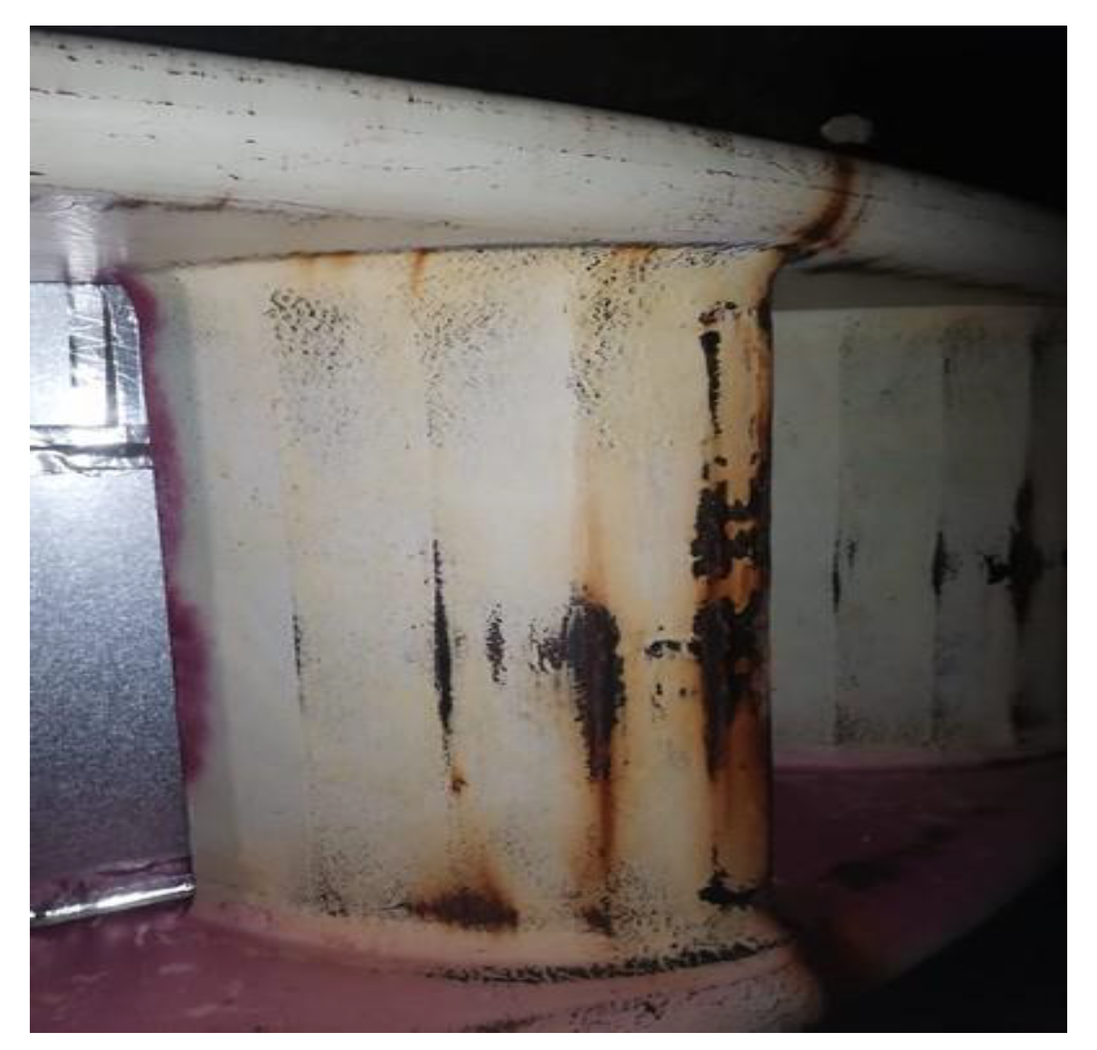
Figure 2.
A damaged cover.
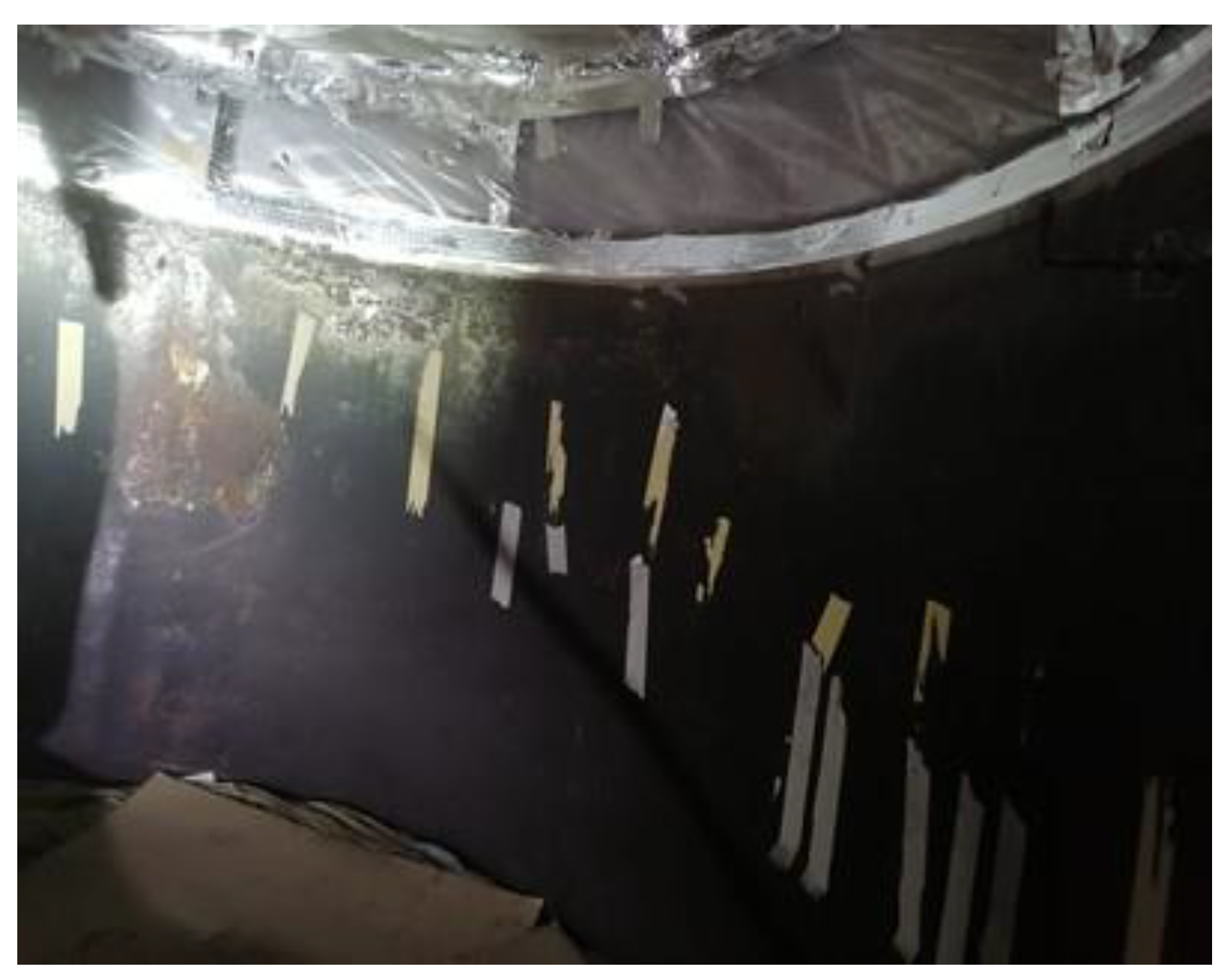
Figure 3.
Corrosion/erosion to the spiral casing and stay vanes.
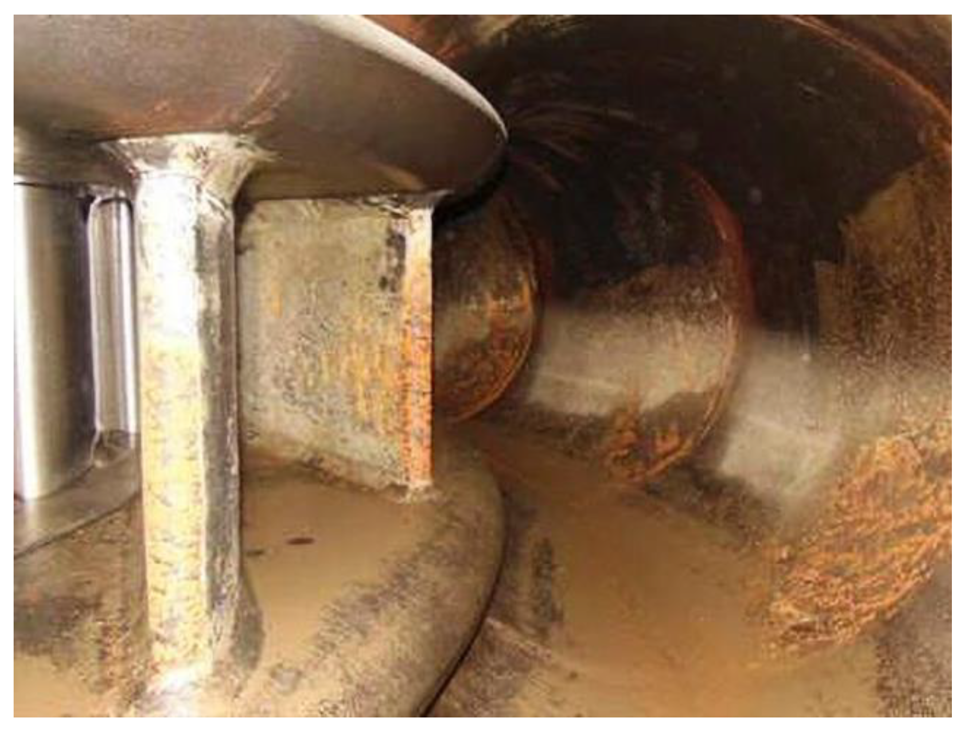
Figure 4.
The skin plate damages of a guided vane of G.M. Shrum, BC Hydro [7].
Figure 4.
The skin plate damages of a guided vane of G.M. Shrum, BC Hydro [7].
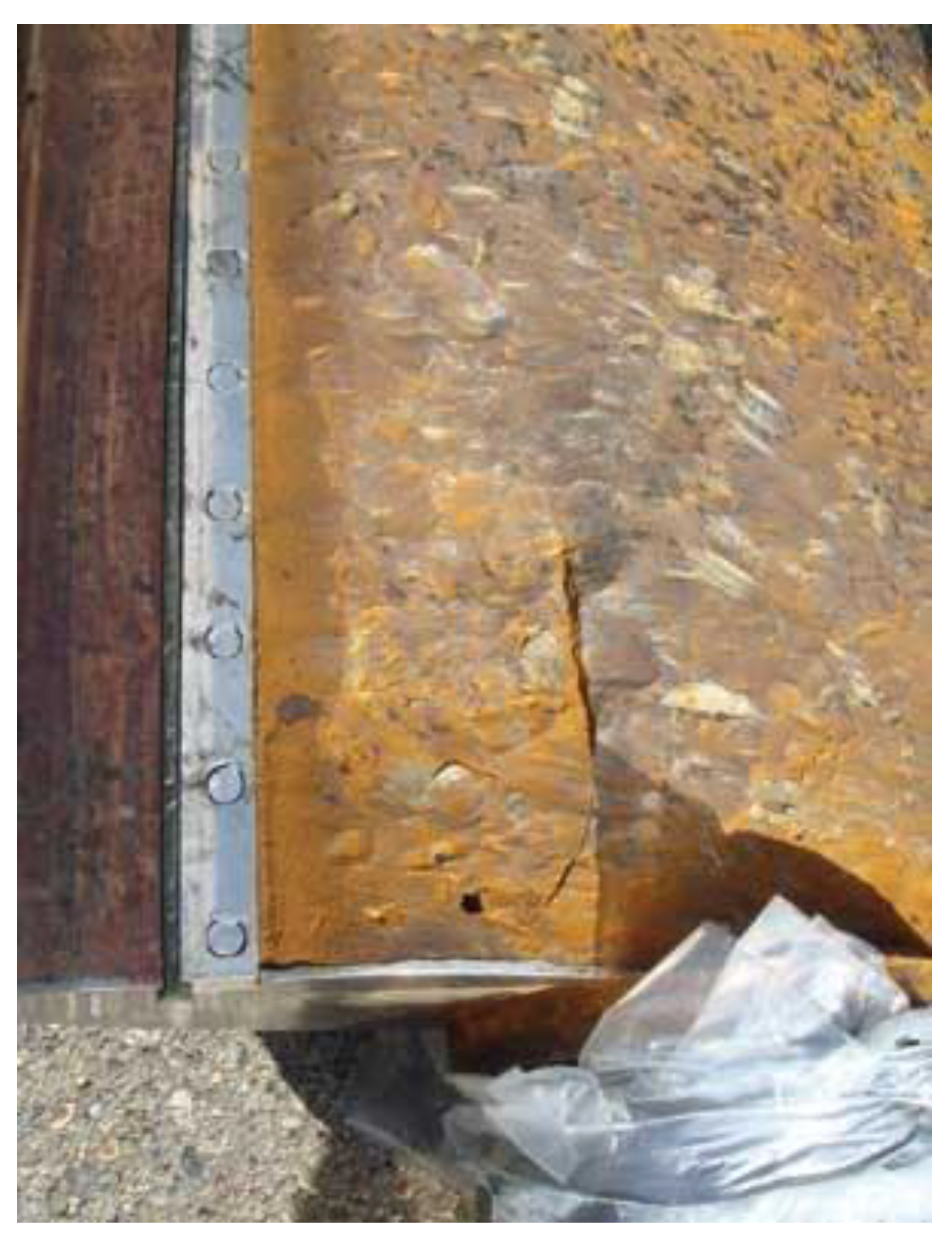
Figure 5.
The water flow of a Francis turbine stay vanes [10]: (a) before optimization; (b) after optimization.
Figure 5.
The water flow of a Francis turbine stay vanes [10]: (a) before optimization; (b) after optimization.
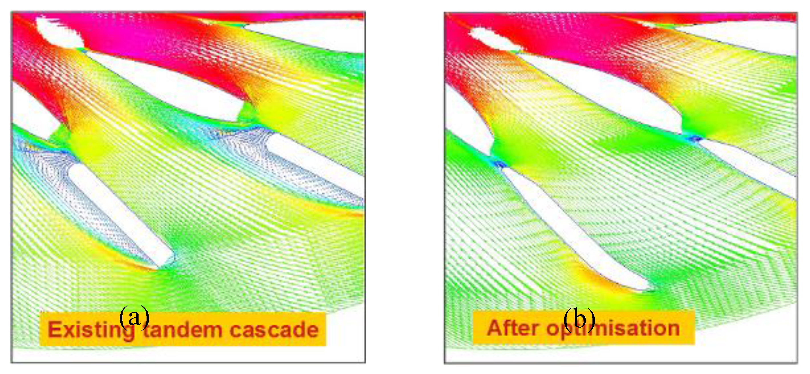
Figure 6.
Francis turbine: (а) The cover ring; (b) Stay ring with stay and guided vanes.
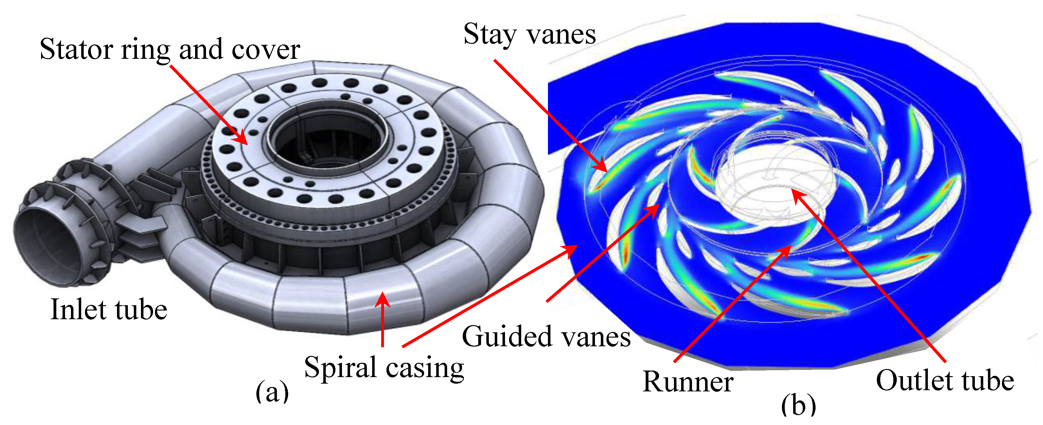
Figure 7.
Three cases of the stay vanes examined: (a) Original shape; (b) First stage of reshaping; (c) Final stage of reshaping.
Figure 7.
Three cases of the stay vanes examined: (a) Original shape; (b) First stage of reshaping; (c) Final stage of reshaping.
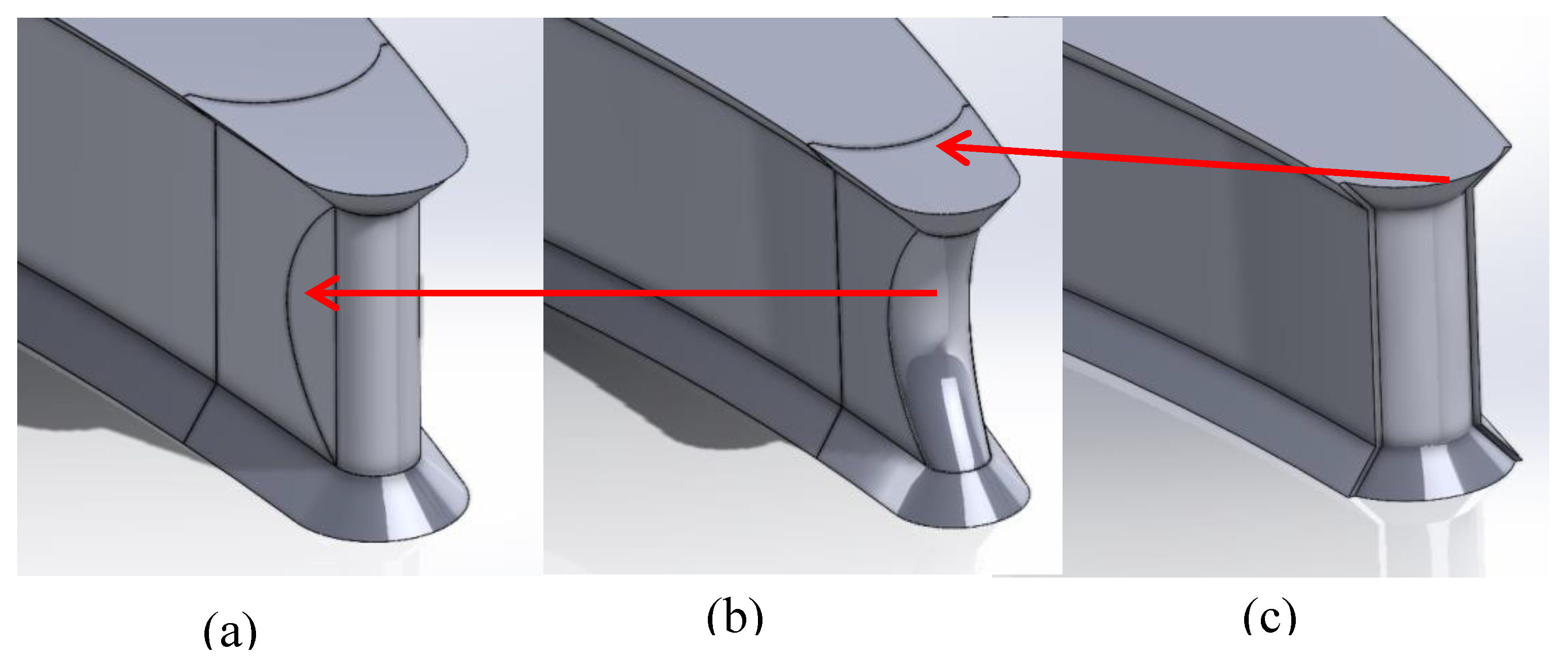
Figure 8.
The stay ring and runner finite element distribution.
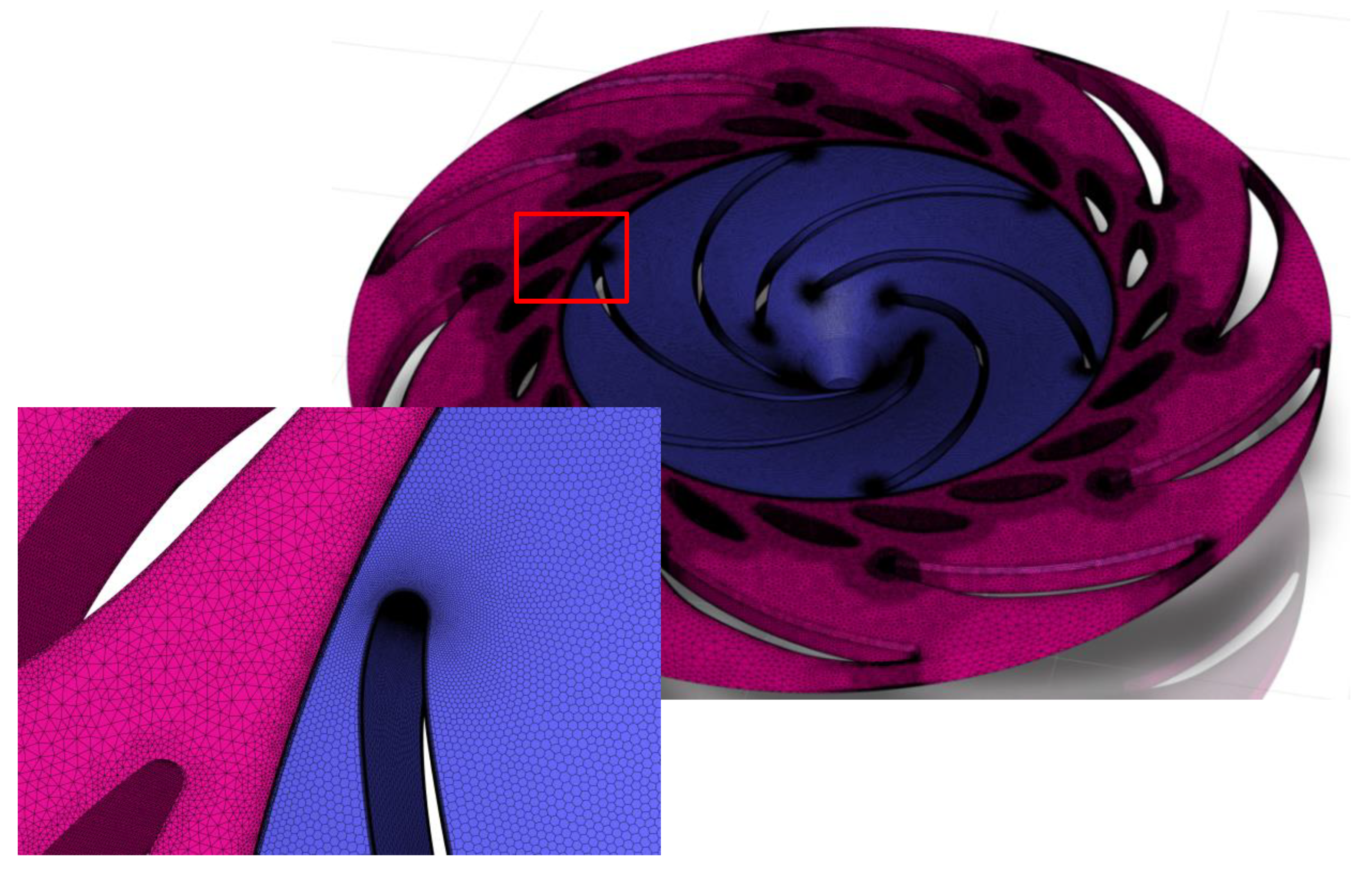
Figure 9.
The finite element distribution of a part of a stay vane and of its adjacent surface.
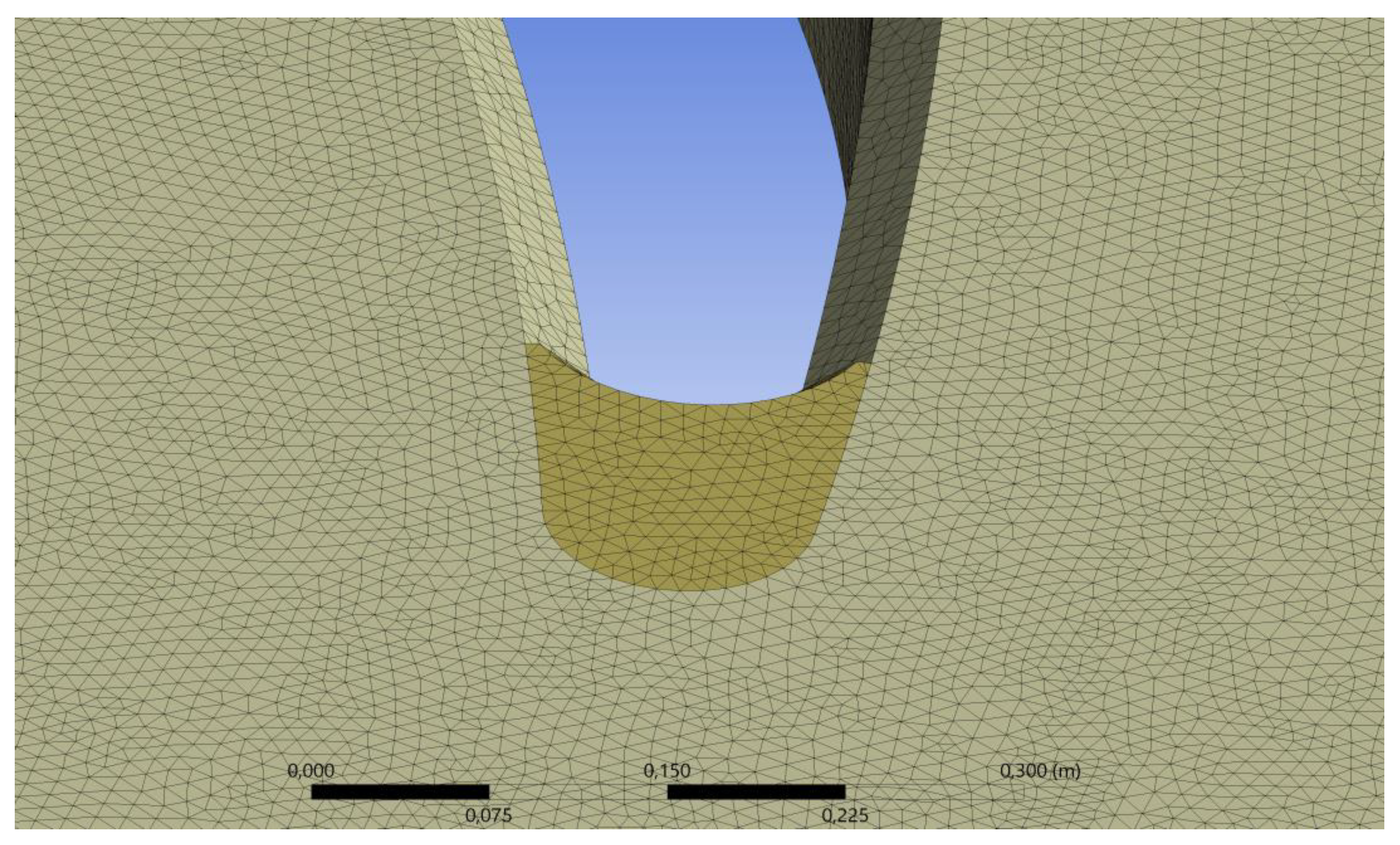
Figure 10.
The areas with the densest and precise finite element distribution of a stay vane and the parts of its reshaping: (a) Variant I; (b) Variant II; (c) Variant III.
Figure 10.
The areas with the densest and precise finite element distribution of a stay vane and the parts of its reshaping: (a) Variant I; (b) Variant II; (c) Variant III.
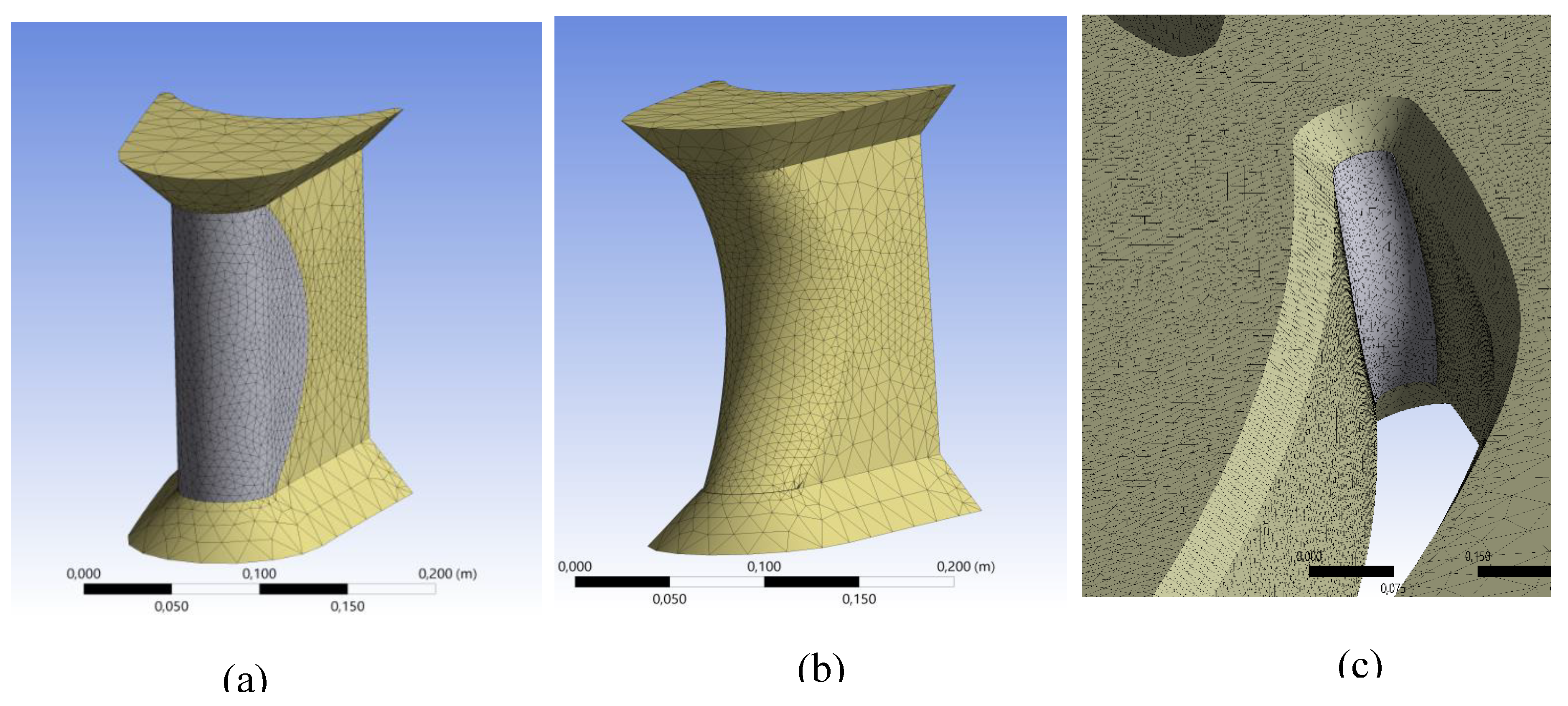
Figure 11.
Distribution of the total pressure [Pa] along the contour of the stay vanes in generator mode: (a) Variant I; (b) Variant II; (c) Variant III.
Figure 11.
Distribution of the total pressure [Pa] along the contour of the stay vanes in generator mode: (a) Variant I; (b) Variant II; (c) Variant III.
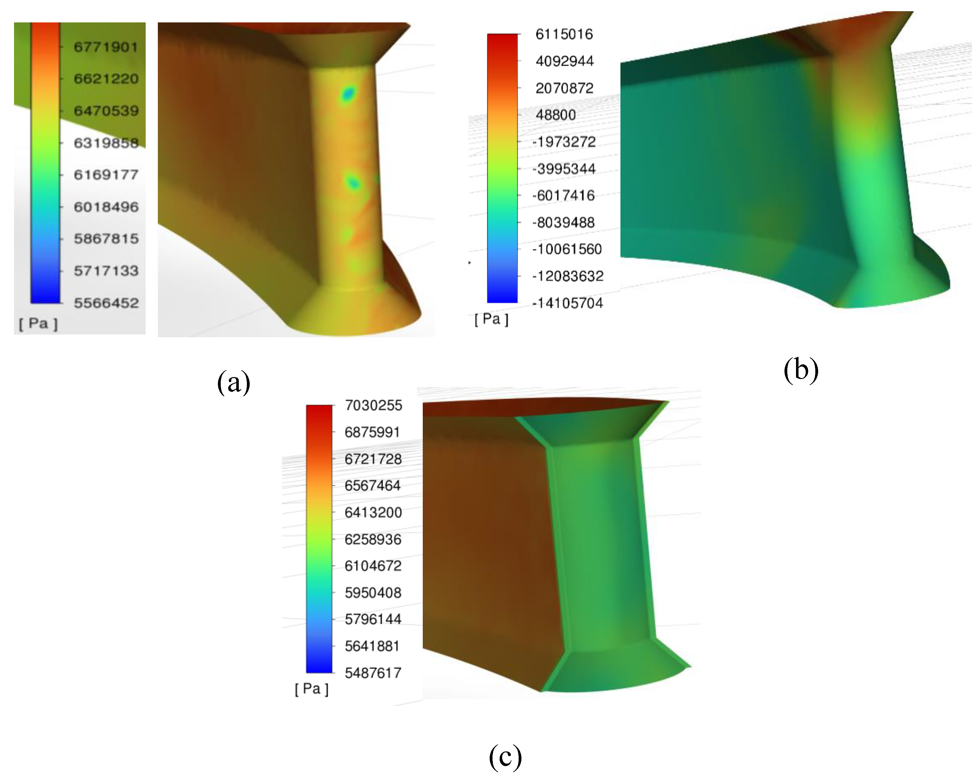
Figure 12.
Distribution of the total pressure [Pa] along the contour of the stay vanes in pump mode: (a) Variant I; (b) Variant II; (c) Variant III.
Figure 12.
Distribution of the total pressure [Pa] along the contour of the stay vanes in pump mode: (a) Variant I; (b) Variant II; (c) Variant III.
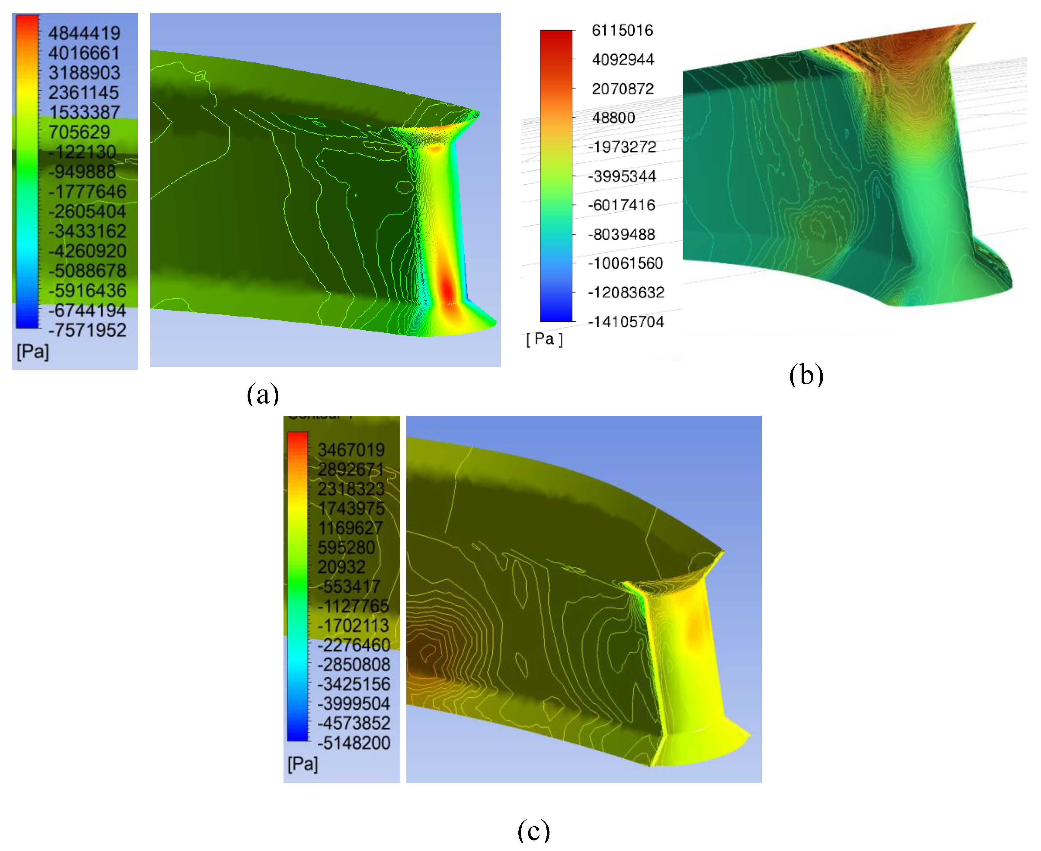
Figure 13.
The stay and guided vanes; (a) 3D volumes of the stay and guided vanes, and the runner; (b) the plane Z – Y along the runner axes.
Figure 13.
The stay and guided vanes; (a) 3D volumes of the stay and guided vanes, and the runner; (b) the plane Z – Y along the runner axes.
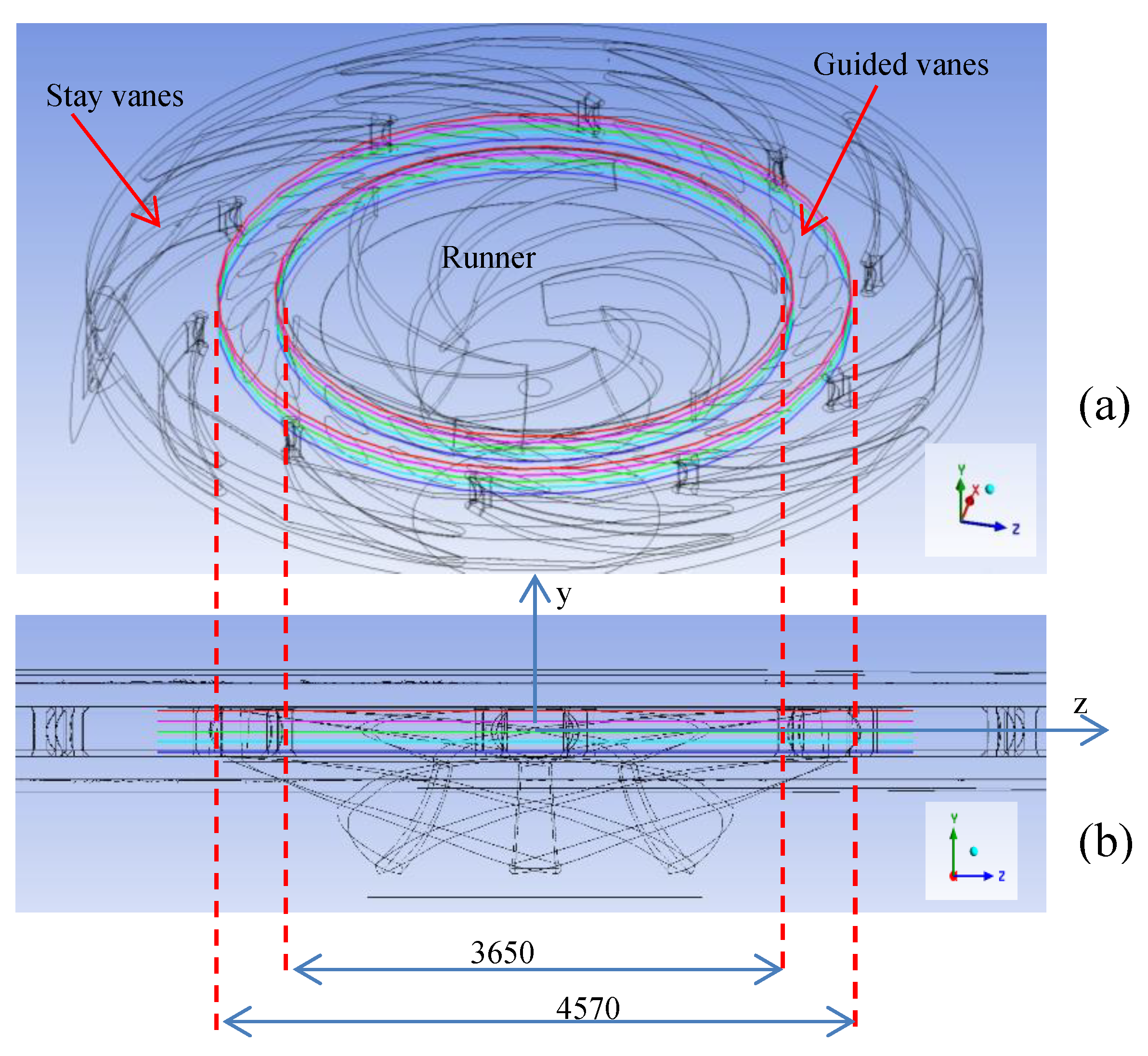
Figure 14.
Velocity (m/s) distribution of the flow through the flow section in the plane y = −0.1 m in generator mode: (a) Variant I; (b) Variant II; (c) Variant III.
Figure 14.
Velocity (m/s) distribution of the flow through the flow section in the plane y = −0.1 m in generator mode: (a) Variant I; (b) Variant II; (c) Variant III.
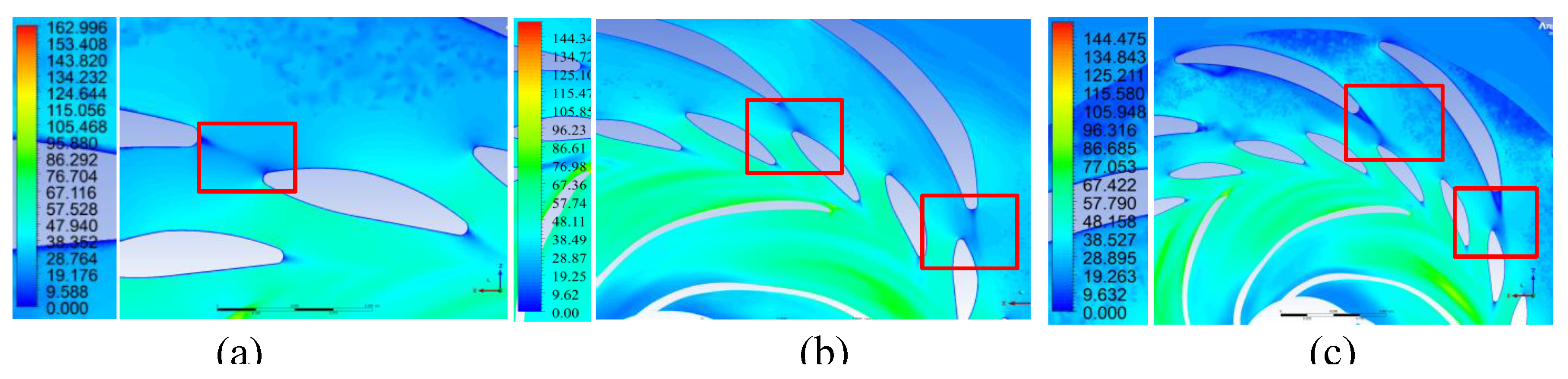
Figure 15.
Flow velocity (m/s) vectors through the flow section in the plane y = −0.1 m in generator mode: (a) Variant I; (b) Variant II; (c) Variant III.
Figure 15.
Flow velocity (m/s) vectors through the flow section in the plane y = −0.1 m in generator mode: (a) Variant I; (b) Variant II; (c) Variant III.
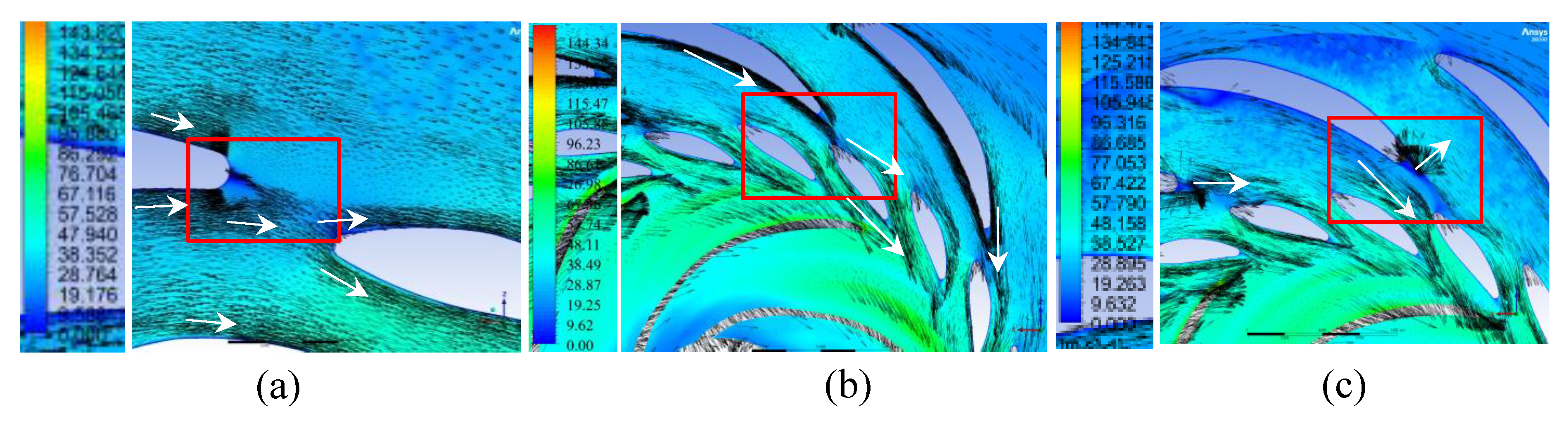
Figure 16.
Velocity (m/s) distribution of the flow through the flow section in the plane y = -0.05 m in generator mode: (a) Variant I; (b) Variant II; (c) Variant III.
Figure 16.
Velocity (m/s) distribution of the flow through the flow section in the plane y = -0.05 m in generator mode: (a) Variant I; (b) Variant II; (c) Variant III.
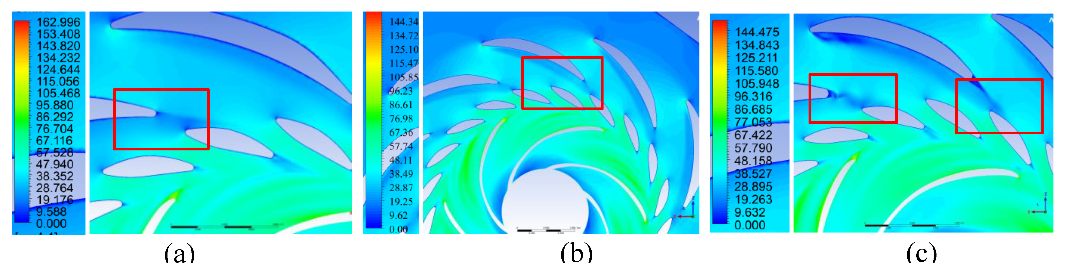
Figure 17.
Velocity (m/s) vectors through the flow section in the plane y = -0.05 m in generator mode: (a) Variant I; (b) Variant II; (c) Variant III.
Figure 17.
Velocity (m/s) vectors through the flow section in the plane y = -0.05 m in generator mode: (a) Variant I; (b) Variant II; (c) Variant III.
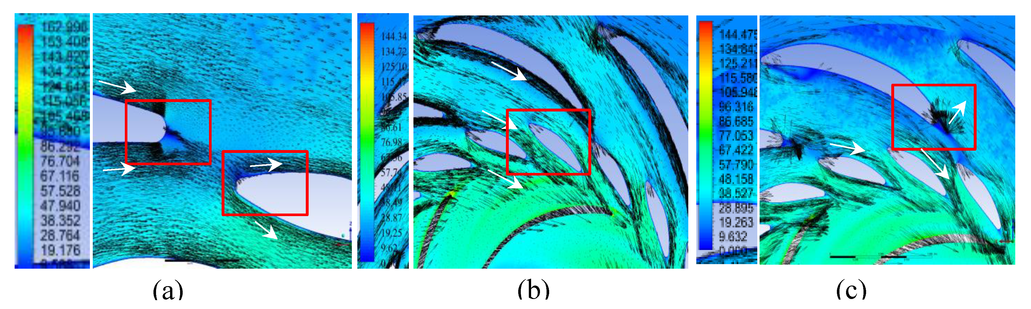
Figure 18.
Velocity m/s distribution of the flow through the flow section in the plane y = 0 m in generator mode: (a) Variant I; (b) Variant II; (c) Variant III.
Figure 18.
Velocity m/s distribution of the flow through the flow section in the plane y = 0 m in generator mode: (a) Variant I; (b) Variant II; (c) Variant III.
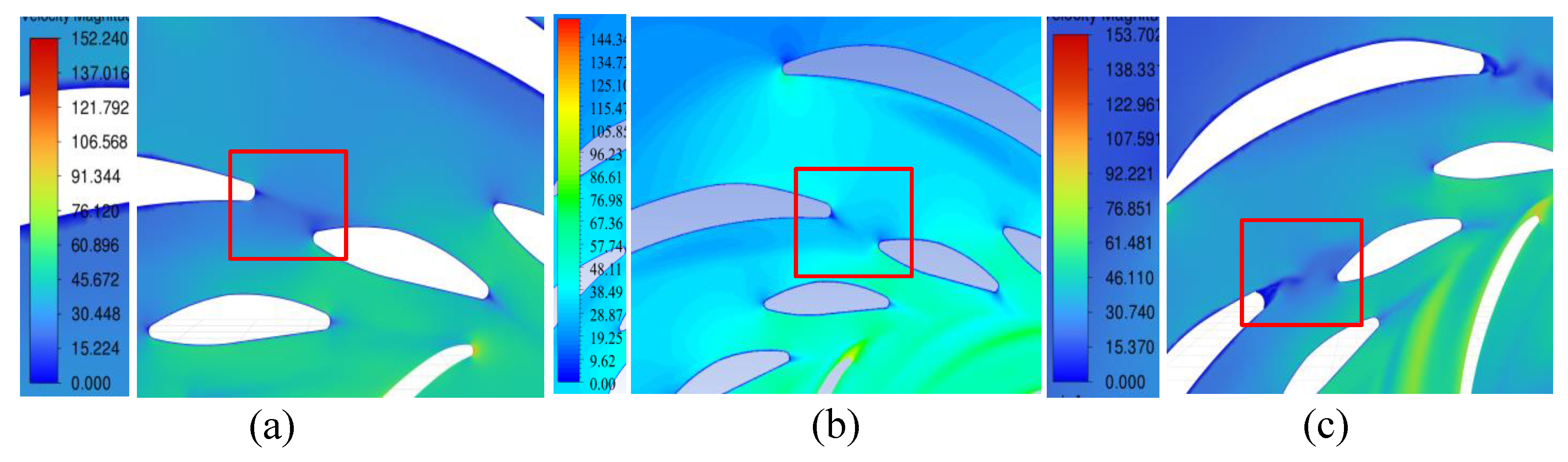
Figure 19.
Flow velocity (m/s) vectors through the flow section in the plane y = 0 m in generator mode: (a) Variant I; (b) Variant II; (c) Variant III.
Figure 19.
Flow velocity (m/s) vectors through the flow section in the plane y = 0 m in generator mode: (a) Variant I; (b) Variant II; (c) Variant III.
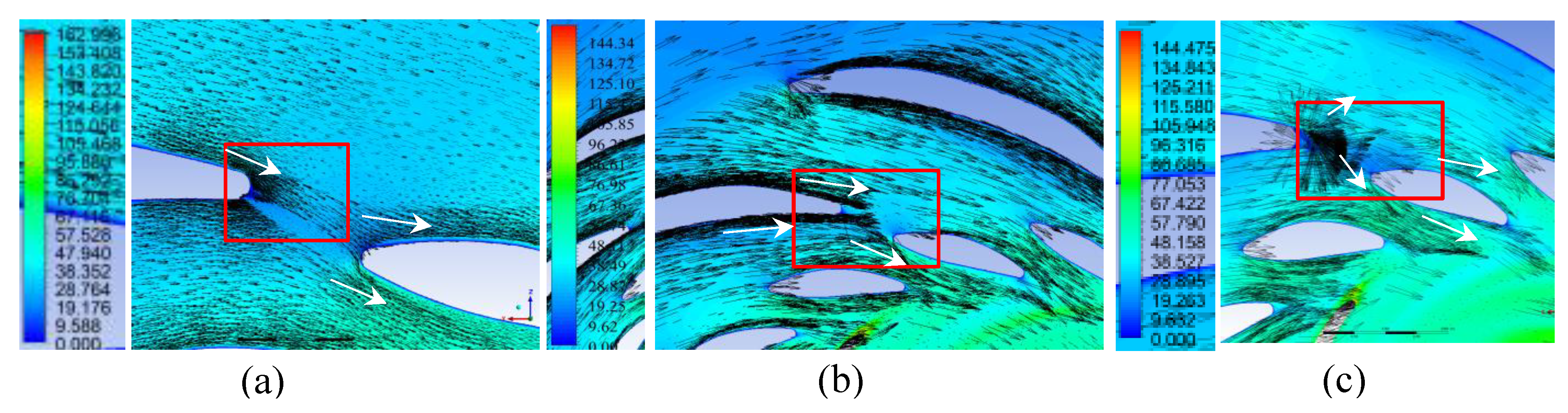
Figure 20.
Velocity (m/s) distribution of the flow through the flow section in the plane y = 0.05 m in generator mode: (a) Variant I; (b) Variant II; (c) Variant III.
Figure 20.
Velocity (m/s) distribution of the flow through the flow section in the plane y = 0.05 m in generator mode: (a) Variant I; (b) Variant II; (c) Variant III.
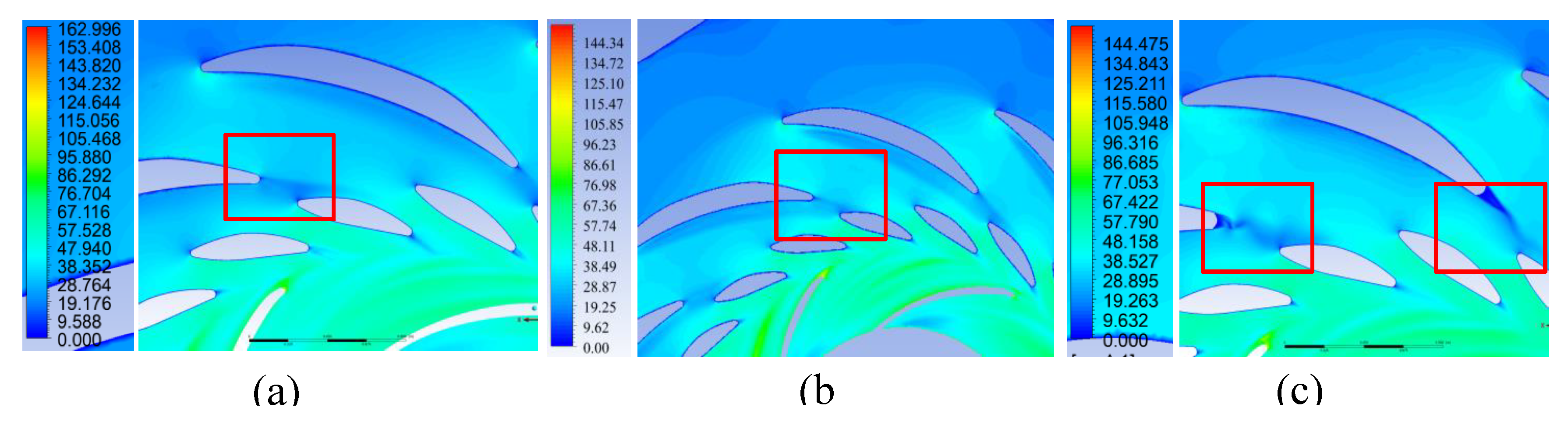
Figure 21.
Flow velocity (m/s) vectors through the flow section in the plane y = 0.05 m in generator mode: (a) Variant I; (b) Variant II; (c) Variant III.
Figure 21.
Flow velocity (m/s) vectors through the flow section in the plane y = 0.05 m in generator mode: (a) Variant I; (b) Variant II; (c) Variant III.
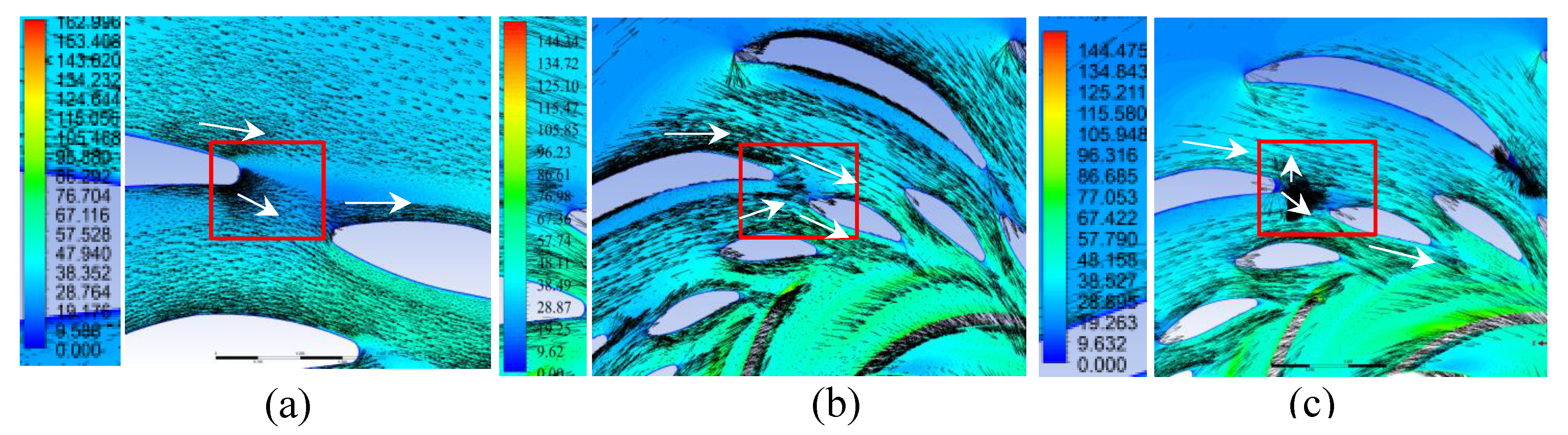
Figure 22.
Velocity (m/s) distribution of the flow through the flow section in the plane y = 0.1 m in generator mode: (a) Variant I; (b) Variant II; (c) Variant III.
Figure 22.
Velocity (m/s) distribution of the flow through the flow section in the plane y = 0.1 m in generator mode: (a) Variant I; (b) Variant II; (c) Variant III.
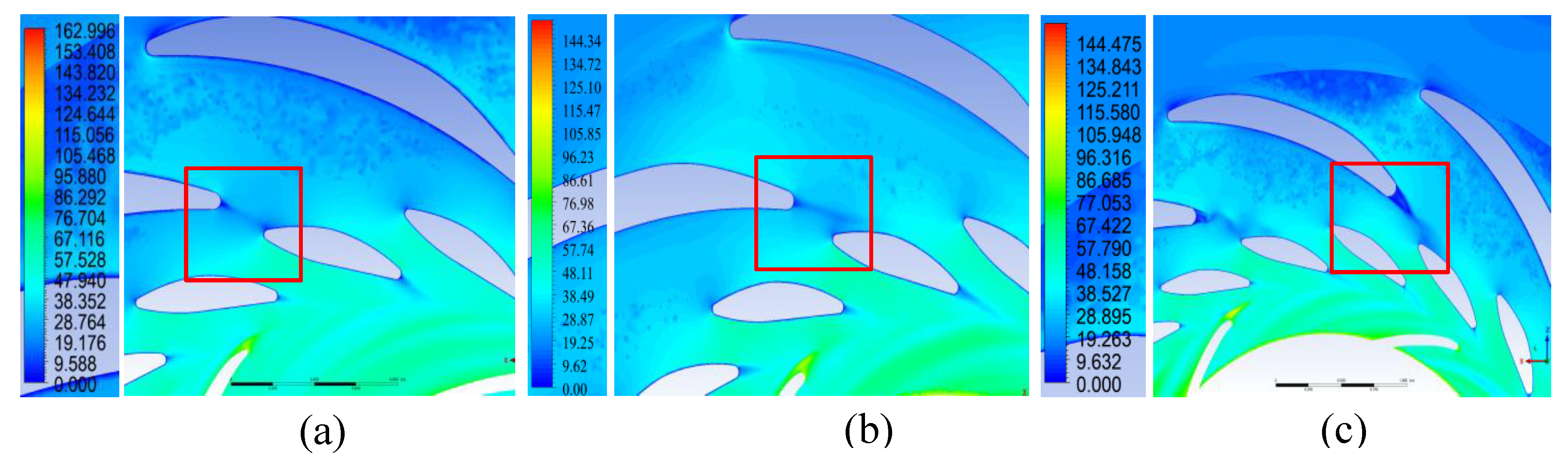
Figure 23.
Flow velocity (m/s) vectors through the flow section in the plane y = 0.1 m in generator mode: (a) Variant I; (b) Variant II; (c) Variant III.
Figure 23.
Flow velocity (m/s) vectors through the flow section in the plane y = 0.1 m in generator mode: (a) Variant I; (b) Variant II; (c) Variant III.
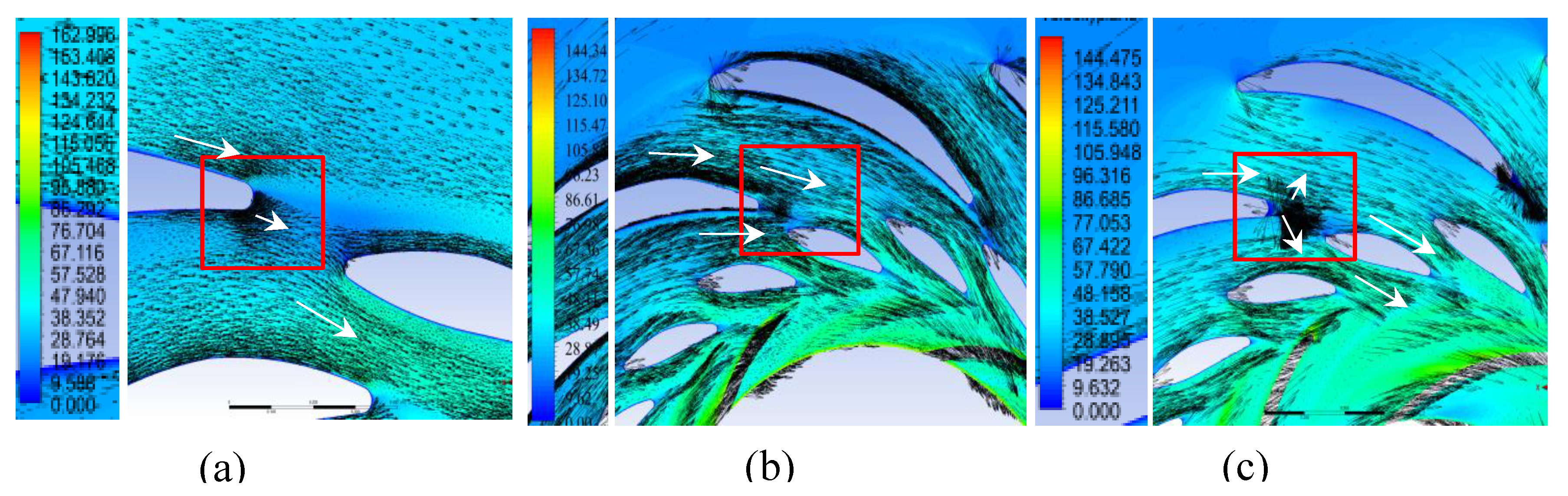
Figure 24.
Velocity (m/s) distribution of the flow through the flow section in the plane y = −0.1 m in pump mode: Variant I; Variant II; Variant III.
Figure 24.
Velocity (m/s) distribution of the flow through the flow section in the plane y = −0.1 m in pump mode: Variant I; Variant II; Variant III.
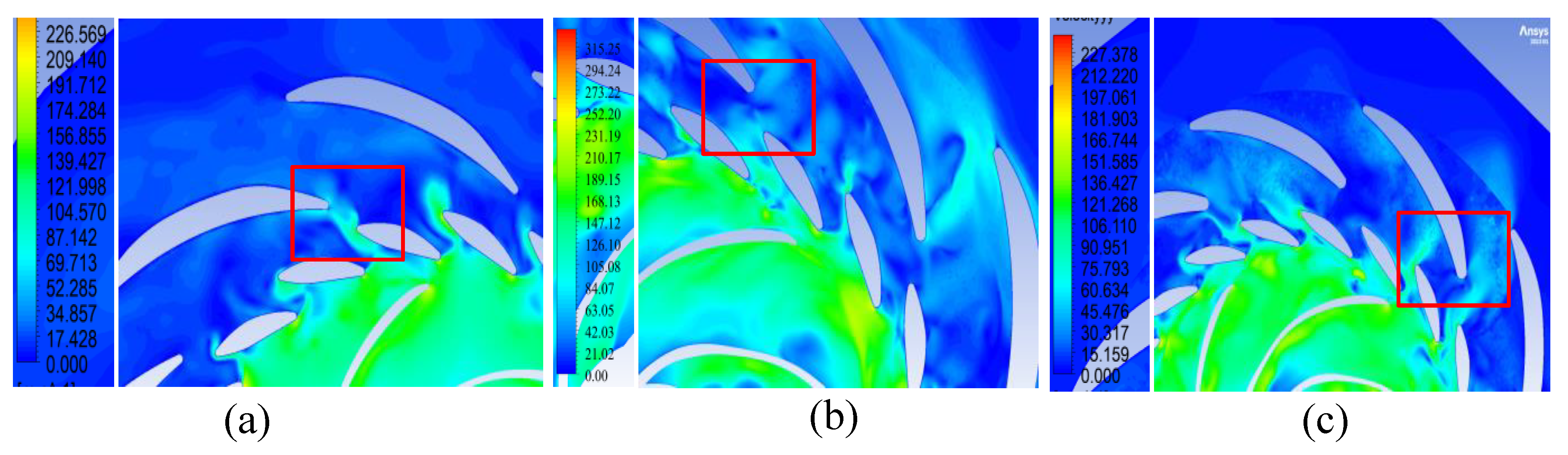
Figure 25.
Flow velocity (m/s) vectors through the flow section in the plane y = −0.1 m in pump mode: Variant I; Variant II; Variant III.
Figure 25.
Flow velocity (m/s) vectors through the flow section in the plane y = −0.1 m in pump mode: Variant I; Variant II; Variant III.
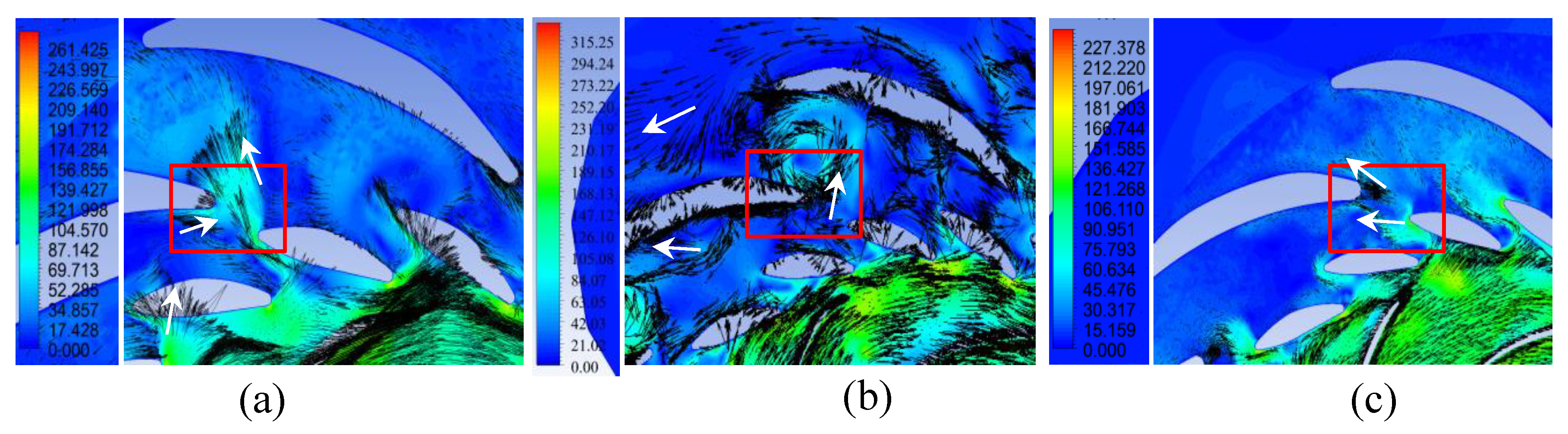
Figure 26.
Velocity (m/s) distribution of the flow through the flow section in the plane y = -0.05 m in pump mode: Variant I; Variant II; Variant III.
Figure 26.
Velocity (m/s) distribution of the flow through the flow section in the plane y = -0.05 m in pump mode: Variant I; Variant II; Variant III.
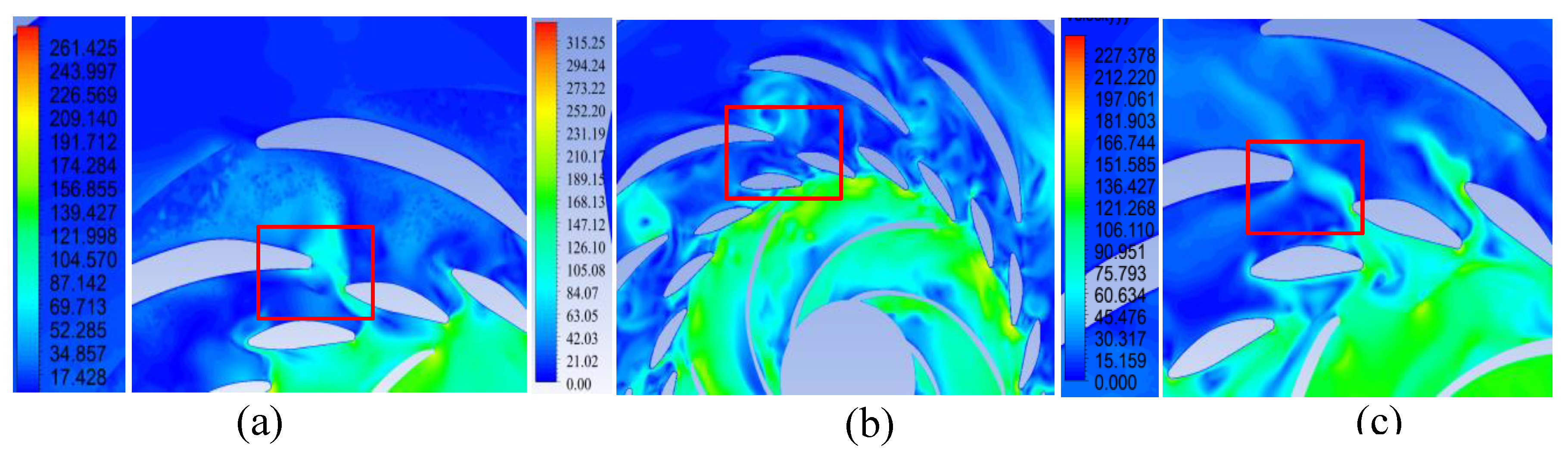
Figure 27.
Velocity (m/s) vectors through the flow section in the plane y = -0.05 m in pump mode: Variant I; Variant II; Variant III.
Figure 27.
Velocity (m/s) vectors through the flow section in the plane y = -0.05 m in pump mode: Variant I; Variant II; Variant III.
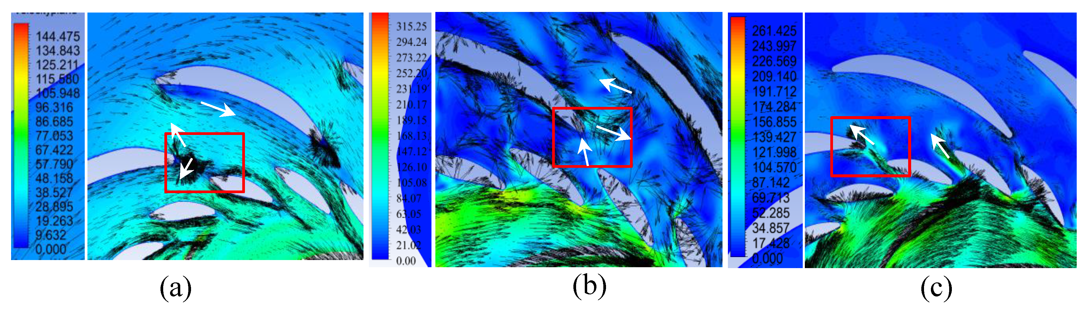
Figure 28.
Velocity m/s distribution of the flow through the flow section in the plane y = 0 m in pump mode: Variant I; Variant II; Variant III.
Figure 28.
Velocity m/s distribution of the flow through the flow section in the plane y = 0 m in pump mode: Variant I; Variant II; Variant III.
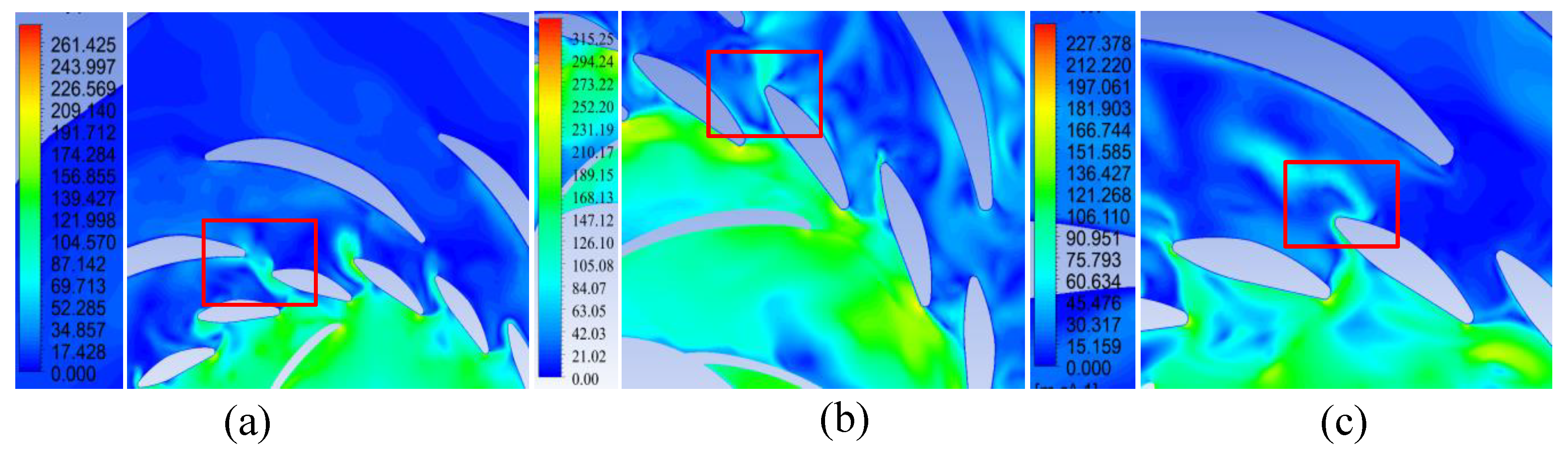
Figure 29.
Flow velocity (m/s) vectors through the flow section in the plane y = 0 m in pump mode: Variant I; Variant II; Variant III.
Figure 29.
Flow velocity (m/s) vectors through the flow section in the plane y = 0 m in pump mode: Variant I; Variant II; Variant III.
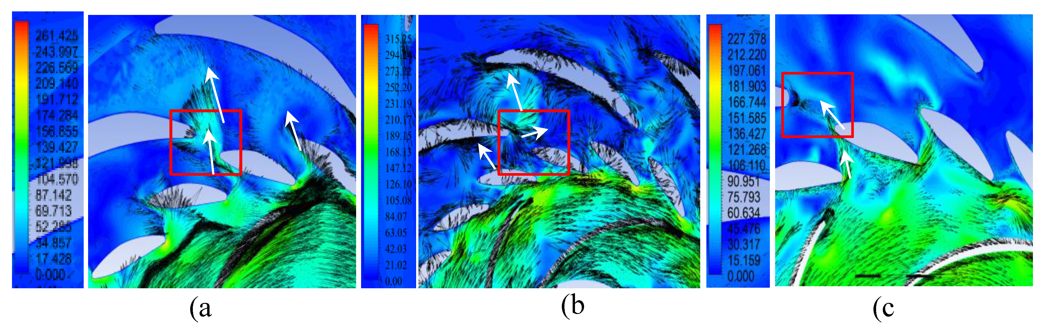
Figure 30.
Velocity (m/s) distribution of the flow through the flow section in the plane y = 0.05 m in pump mode: Variant I; Variant II; Variant III.
Figure 30.
Velocity (m/s) distribution of the flow through the flow section in the plane y = 0.05 m in pump mode: Variant I; Variant II; Variant III.

Figure 31.
Flow velocity (m/s) vectors through the flow section in the plane y = 0.05 m in pump mode: Variant I; Variant II; Variant III.
Figure 31.
Flow velocity (m/s) vectors through the flow section in the plane y = 0.05 m in pump mode: Variant I; Variant II; Variant III.
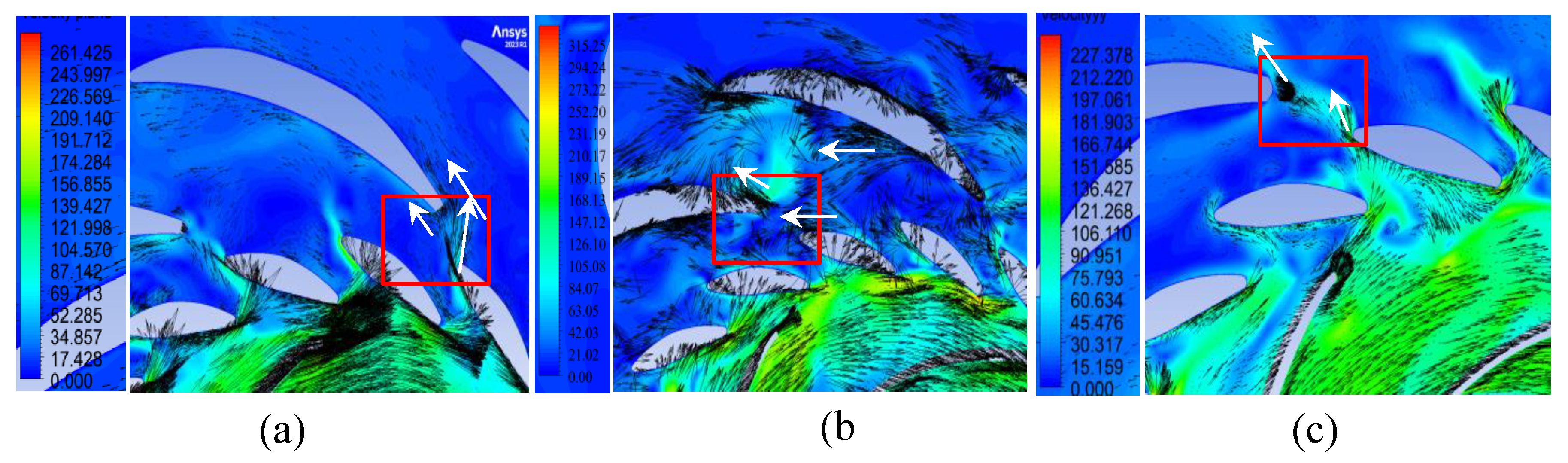
Figure 32.
Velocity (m/s) distribution of the flow through the flow section in the plane y = 0.1 m in pump mode: Variant I; Variant II; Variant III.
Figure 32.
Velocity (m/s) distribution of the flow through the flow section in the plane y = 0.1 m in pump mode: Variant I; Variant II; Variant III.

Figure 33.
Flow velocity (m/s) vectors through the flow section in the plane y = 0.1 m in pump mode: Variant I; Variant II; Variant III.
Figure 33.
Flow velocity (m/s) vectors through the flow section in the plane y = 0.1 m in pump mode: Variant I; Variant II; Variant III.
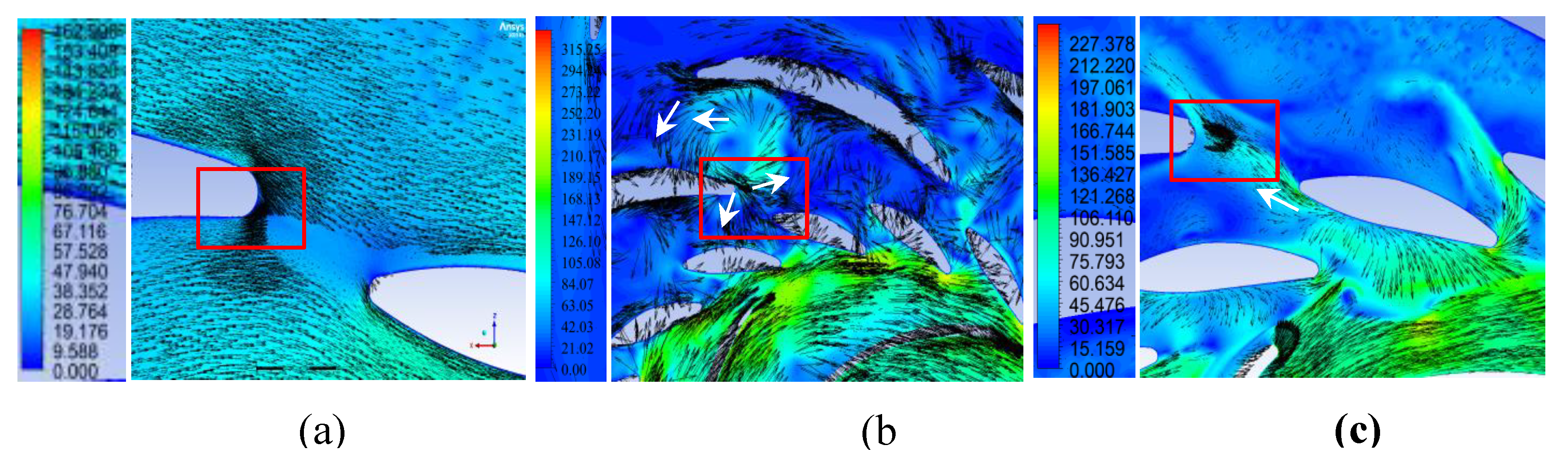
Figure 34.
Velocity distribution along the contour of a circle with a diameter of 3650 mm in generator mode: (a) Variant I; (b) Variant II; (c) Variant III.
Figure 34.
Velocity distribution along the contour of a circle with a diameter of 3650 mm in generator mode: (a) Variant I; (b) Variant II; (c) Variant III.
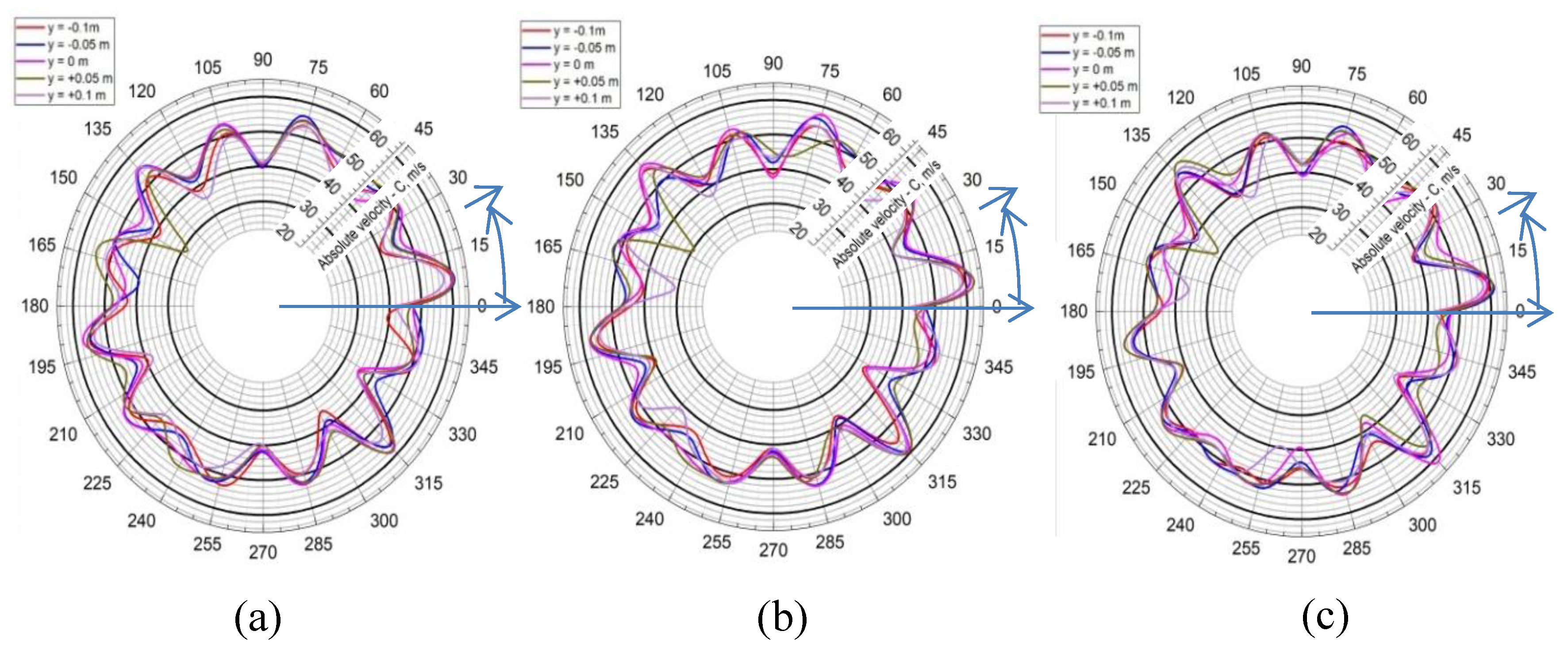
Figure 35.
Velocity distribution along the contour of a circle with a diameter of 4570 mm in generator mode: (a) Variant I; (b) Variant II; (c) Variant III.
Figure 35.
Velocity distribution along the contour of a circle with a diameter of 4570 mm in generator mode: (a) Variant I; (b) Variant II; (c) Variant III.
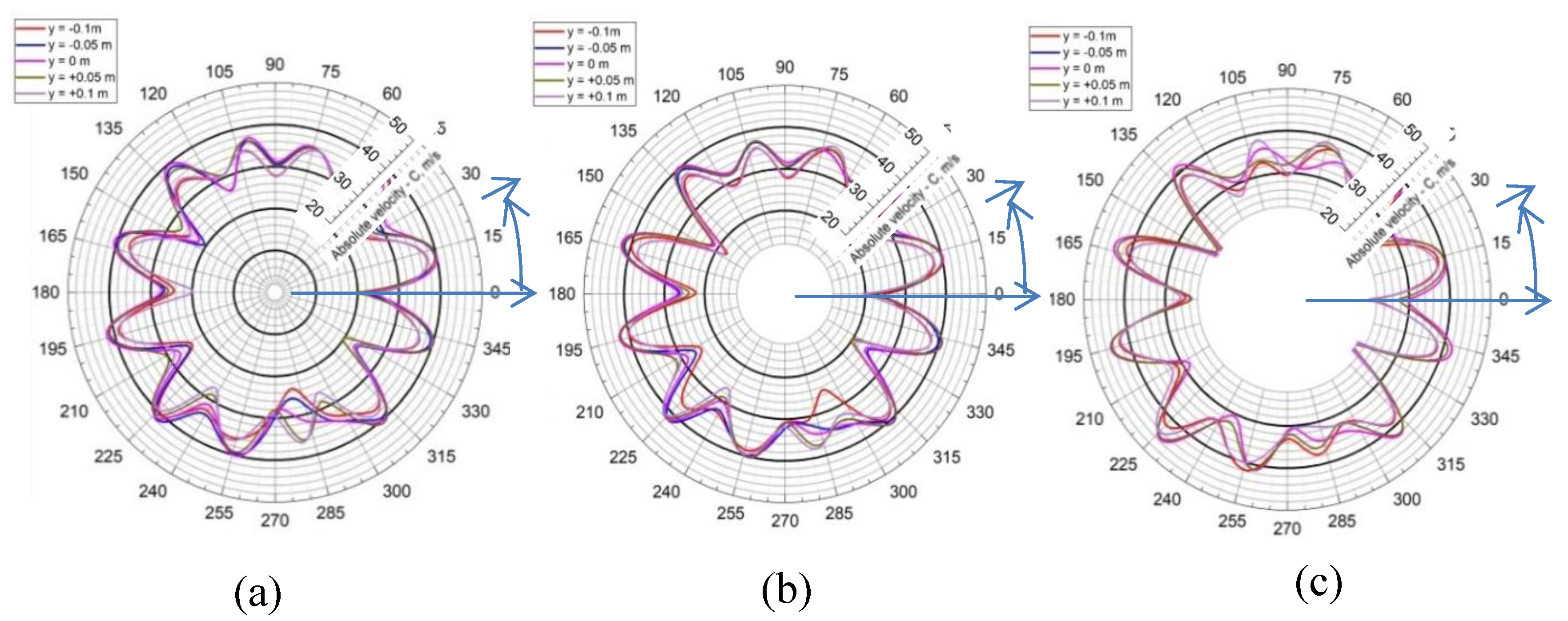
Figure 36.
Velocity distribution along the contour of a circle with a diameter of 3650 mm in pump mode: (a) Variant I; (b) Variant II; (c) Variant III.
Figure 36.
Velocity distribution along the contour of a circle with a diameter of 3650 mm in pump mode: (a) Variant I; (b) Variant II; (c) Variant III.
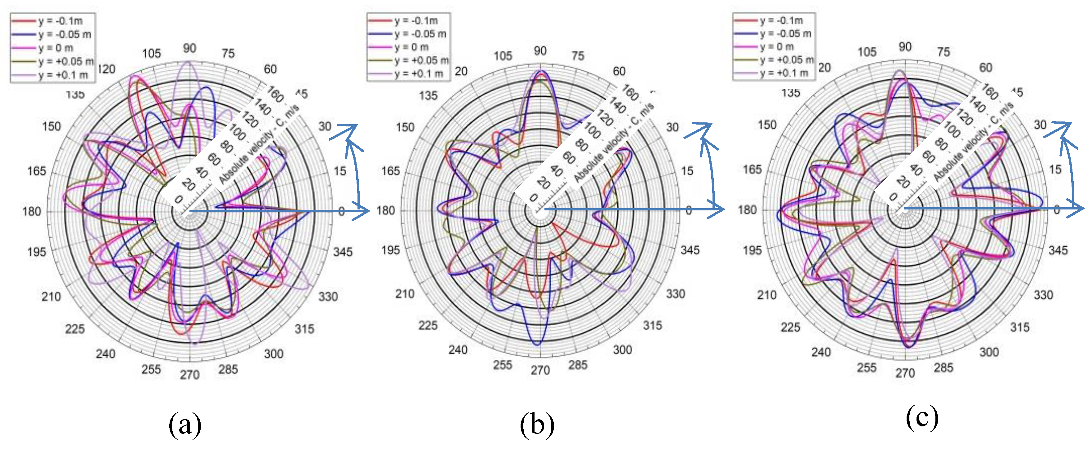
Figure 37.
Velocity distribution along the contour of a circle with a diameter of 4570 mm in pump mode: (a) Variant I; (b) Variant II; (c) Variant III.
Figure 37.
Velocity distribution along the contour of a circle with a diameter of 4570 mm in pump mode: (a) Variant I; (b) Variant II; (c) Variant III.
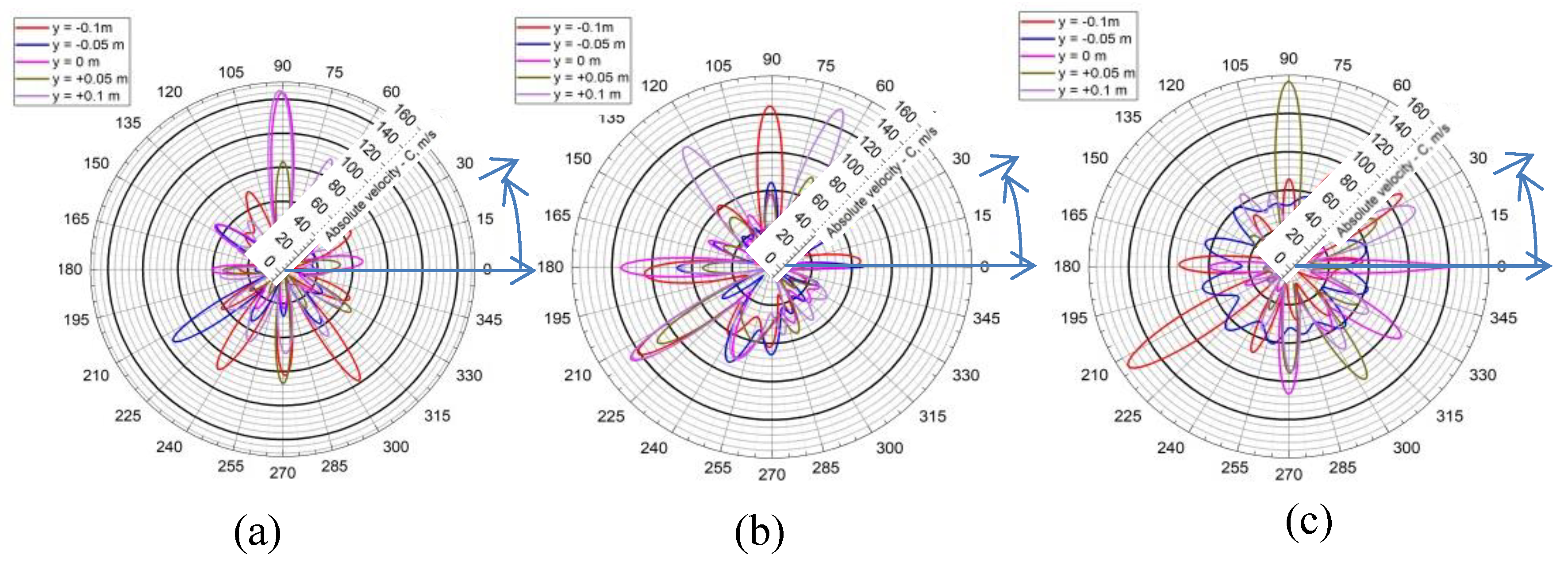
Figure 38.
The process of convergence of results (computation of the torques) in dependence on the iterative procedure of the numerical integration process: (a) generator mode; (b) pump mode.
Figure 38.
The process of convergence of results (computation of the torques) in dependence on the iterative procedure of the numerical integration process: (a) generator mode; (b) pump mode.
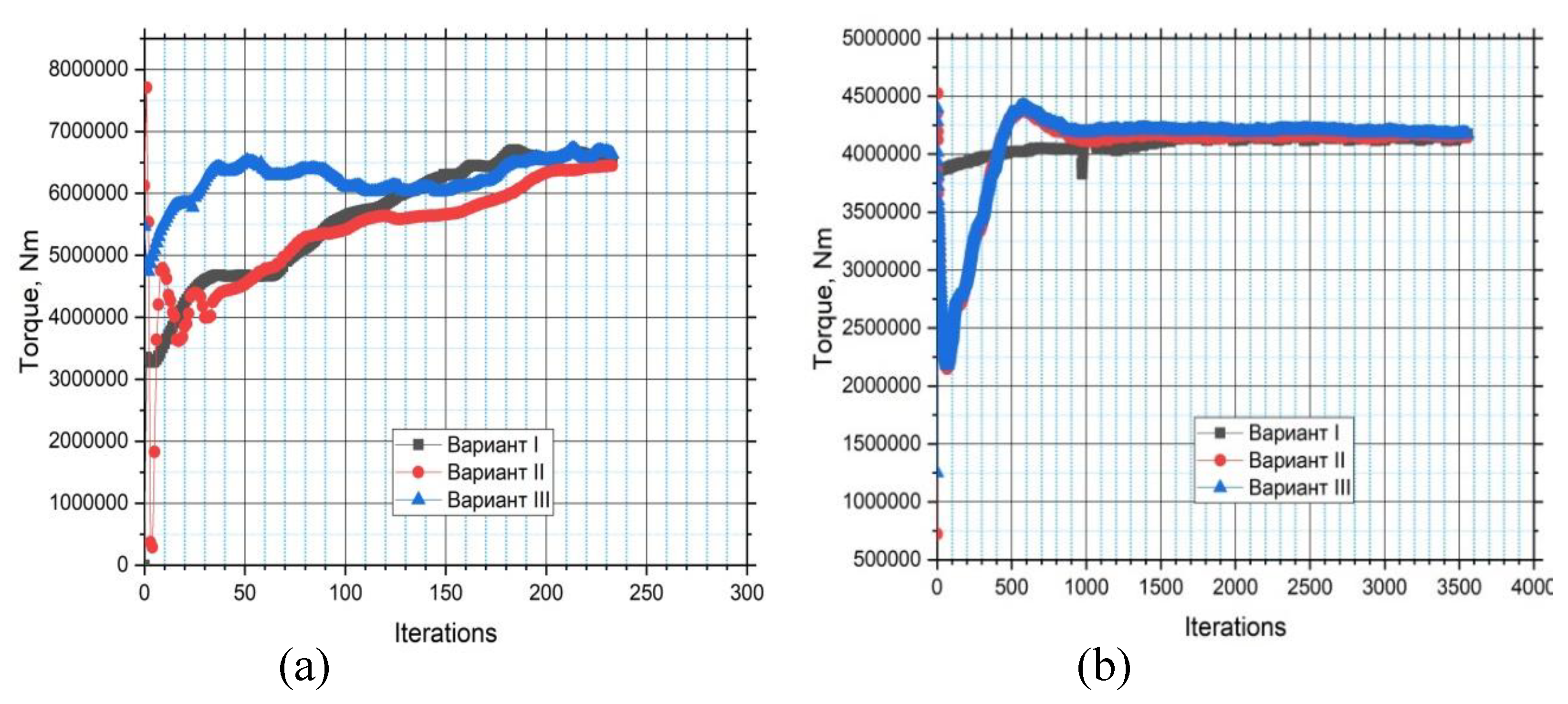
Table 1.
Mesh distribution for different stages of the stay vane repair.
| Objects examined | Number of the cels | Cels type | Minimal orthogonal quality | Maximal geometric ratio |
|---|---|---|---|---|
| 1. Stay ring Figure 7a | 14 592 094 | Tetrahedral | 0.172 | 21 |
| 2. Stay ring Figure 7b | 30 361 924 | Tetrahedral | 0.171 | 21 |
| 3. Stay ring Figure 7c | 49 615 394 | Tetrahedral | 0.172 | 21 |
Table 3.
Average speeds along the contours of a circle with a diameter of 3650 mm (in front of the runner) when the turbine operates in generator mode.
Table 3.
Average speeds along the contours of a circle with a diameter of 3650 mm (in front of the runner) when the turbine operates in generator mode.
| Height y [m] |
C [m/s] | ||
|---|---|---|---|
| Variant I | Вариант II | Variant III | |
| -0.1 | 78.608 | 83.806 | 95.222 |
| -0.05 | 75.477 | 53.841 | 61.831 |
| 0 | 104.137 | 84.994 | 82.076 |
| 0.05 | 71.631 | 68.977 | 96.882 |
| 0.1 | 103.957 | 89.555 | 65.915 |
Table 4.
Average speeds along the contours of a circle with a diameter of 4570 mm (in front of the guided blades) when the turbine operates in generator mode.
Table 4.
Average speeds along the contours of a circle with a diameter of 4570 mm (in front of the guided blades) when the turbine operates in generator mode.
| Height y [m] |
C [m/s] | ||
|---|---|---|---|
| Variant I | Вариант II | Variant III | |
| -0.1 | 42.136 | 83.806 | 39.942 |
| -0.05 | 44.764 | 53.841 | 41.153 |
| 0 | 44.974 | 84.994 | 41.311 |
| 0.05 | 44.764 | 68.977 | 41.004 |
| 0.1 | 44.510 | 89.555 | 39.795 |
Table 5.
Average speeds along the contours of a circle with a diameter of 3650 mm (in front of the impeller) when the turbine operates in pump mode.
Table 5.
Average speeds along the contours of a circle with a diameter of 3650 mm (in front of the impeller) when the turbine operates in pump mode.
| Height y [m] |
C [m/s] | ||
|---|---|---|---|
| Variant I | Вариант II | Variant III | |
| -0.1 | 151.136 | 166.699 | 151.606 |
| -0.05 | 145.862 | 171.066 | 134.351 |
| 0 | 138.594 | 171.646 | 156.430 |
| 0.05 | 143.136 | 157.649 | 148.740 |
| 0.1 | 140.760 | 171.646 | 158.270 |
Table 6.
Average speeds along the contours of a circle with a diameter of 4570 mm (in front of the guided vanes) when the turbine operates in pump mode.
Table 6.
Average speeds along the contours of a circle with a diameter of 4570 mm (in front of the guided vanes) when the turbine operates in pump mode.
| Height y [m] |
C [m/s] | ||
|---|---|---|---|
| Variant I | Вариант II | Variant III | |
| -0.1 | 78.608 | 83.806 | 95.222 |
| -0.05 | 75.477 | 53.841 | 61.831 |
| 0 | 104.137 | 84.994 | 82.076 |
| 0.05 | 71.631 | 68.977 | 96.882 |
| 0.1 | 103.957 | 89.555 | 65.915 |
Table 7.
Relative difference between the maximum and minimum average speed over a circle with a diameter of 3650 mm (in front of the runner) in generator mode.
Table 7.
Relative difference between the maximum and minimum average speed over a circle with a diameter of 3650 mm (in front of the runner) in generator mode.
| C, m/s | ||
|---|---|---|
| Variant I, % | Variant II, % | Variant III, % |
| 4.89 | 2.94 | 8.22 |
Table 8.
Relative difference between the maximum and minimum average speed over a circle with a diameter of 4570 mm (in front of the guided vanes) in generator mode.
Table 8.
Relative difference between the maximum and minimum average speed over a circle with a diameter of 4570 mm (in front of the guided vanes) in generator mode.
| C, m/s | ||
|---|---|---|
| Variant I, % | Variant II, % | Variant III, % |
| 3.67 | 7.47 | 6.31 |
Table 9.
Relative difference between the maximum and minimum average speed on a circle with a diameter of 3650 mm (in front of the runner) in pumping mode.
Table 9.
Relative difference between the maximum and minimum average speed on a circle with a diameter of 3650 mm (in front of the runner) in pumping mode.
| C, m/s | ||
|---|---|---|
| Variant I, % | Variant II, % | Variant III, % |
| 8.29 | 8.15 | 15.11 |
Table 10.
Relative difference between the maximum and minimum average speed on a circle with a diameter of 4570 mm (in front of the guided vanes) in pumping mode.
Table 10.
Relative difference between the maximum and minimum average speed on a circle with a diameter of 4570 mm (in front of the guided vanes) in pumping mode.
| C, m/s | ||
|---|---|---|
| Variant I, % | Variant II, % | Variant III, % |
| 31.21 | 39.87 | 36.17 |
Disclaimer/Publisher’s Note: The statements, opinions and data contained in all publications are solely those of the individual author(s) and contributor(s) and not of MDPI and/or the editor(s). MDPI and/or the editor(s) disclaim responsibility for any injury to people or property resulting from any ideas, methods, instructions or products referred to in the content. |
© 2025 by the authors. Licensee MDPI, Basel, Switzerland. This article is an open access article distributed under the terms and conditions of the Creative Commons Attribution (CC BY) license (http://creativecommons.org/licenses/by/4.0/).
Copyright: This open access article is published under a Creative Commons CC BY 4.0 license, which permit the free download, distribution, and reuse, provided that the author and preprint are cited in any reuse.


