Submitted:
04 December 2025
Posted:
05 December 2025
You are already at the latest version
Abstract
Fermion bound states in the core of a line-shaped vortex of a two-dimensional topological superconductor are investigated. The superconducting pairing potential, described in terms of elliptical coordinates, vanishes along a line defect with the two foci at the endpoints. The superconductivity is induced into a topological insulator via proximity effect with a type II s-wave superconductor. The spin and the momentum are perpendicularly locked by the strong spin-orbit coupling via Rashba interaction. A zero-energy Majorana state arises from the Berry phase together with a sequence of equally spaced fermion excitations. By solving the Bogoliubov-de Gennes equations using the method employed by Caroli, de Gennes and Matricon we calculate the energies, the wavefunctions and spin-polarization of the bound states. An analytic expression for the local density of states within the vortex is obtained.
Keywords:
majorana states
; two-dimensional topological superconductor
; line-shaped vortex
1. Introduction
Majorana bound states are unconventional zero-energy quasi-particles with non-Abelian statistics which are their own antiparticles. [1] These states have been proposed for storing quantum information [2] and for fault-tolerant quantum computing. The formation of Majorana bound states at the surface of a strong topological insulator (TI) with superconducting properties in the proximity of an s-wave superconductor (S) has been explored by Fu and Kane [3,4] and Sau et al. [5] Following Refs. [3] and [4] the surface states of a heterostructure in a TI with proximity-induced S were studied in different geometries. [5,6,7,8] The magnitude of the induced superconducting gap depends on the transparency of the TI/S junction and is in general smaller than the parent S gap. For low-lying excitations, the induced gap is a weak function of energy so that can be considered constant. Accordingly the problem is reduced to a 2D topological electron gas with superconducting BCS gap. An alternative platform to generate Majorana zero-energy modes in heterostructures consists of a semiconducting thin film sandwiched between a magnetic insulator and an s-wave superconductor. [9,10] In summary, a Majorana state can arise from a superconducting flux quantum trapped by a defect in a superconducting layer (Abrikosov vortex) [1,11,12,13,14], a layered heterostructure of a magnetic insulator, a semiconductor and a superconductor [9,10], in a tri-junction pair geometry [3,5] or a cylindrical cavity in a 2D superconductor. [7,8,15]
In this paper we investigate a flux quantum trapped in a line-shaped vortex core in a 2D topological superconductor. As a consequence of the geometry, all previously studied cases require polar coordinates, while in the present situation elliptic coordinates are more appropriate.
The electronic structure of in-gap states of a vortex in a 2D topological superconductor has been studied by numerous authors [5,7,8,15,16,17,18,19,20] by solving the corresponding Bogoliubov-de Gennes (BdG) equations. Key is the strong spin-orbit coupling leading to spin-momentum locking and a Berry phase of 1/2. This converts half-integer quantum numbers into integer ones and opens the possibility to create a zero-energy Majorana fermion. For a finite Fermi energy the low-energy excitations are equally spaced by an amount , where is the superconducting gap far away from the vortex. The minigap from the Majorana mode to the first excitation can however be tuned by varying the Fermi energy and for the gap is of the order of . [5,7,12]
Vortex states in superconducting graphene [21] are closely related to vortices with pointlike core in the present problem. The pseudospin parametrizing the two sublattices of the honeycomb lattice plays the role of the spin in the topological insulator. The BdG equations in superconducting graphene for energies close to the Dirac points (considering the spin, pseudospin and particle-holes) reduce to eight equations which decouple into two equivalent subsets of four equations each. Each subset is then equivalent to the present problem for a vortex trapped by a point defect with Dirac interaction. [22]
Analytical expressions for the low-energy bound state eigenvalues, the eigenfunctions and the local density of states (LDOS) for an isolated point vortex with strong spin-orbit coupling have been recently obtained [12,13,15] by solving the BdG equations using the method employed by Caroli, de Gennes and Matricon (CdeGM) [23,24] for a topological type II s-wave superconductor in terms of Bessel functions. The method consists of solving the BdG equations for small distances (compared to the correlation length ) from the core of the vortex, as well as for larger distances (still smaller than ). If the matching condition of these two solutions at an intermediate distance is independent of the distance from the vortex core, then we have a solution for the entire region of the vortex.
Experimentally, systems with large superconducting transition temperature are desirable. A zero-energy mode was detected via spin-selective Andreev reflections in the heterostructure Bi2Te3/NbSe2[25] and with tunneling scanning spectroscopy in monolayers of the high-temperature superconductor FeTe0.55Se0.45. [26,27] To prove that the measured peak corresponds to a Majorana state requires the exchange of two such modes (qubit).
In the present paper we extend the calculation to a line-shaped vortex core (corresponding to a cut in the 2D superconductor confined between two foci) using elliptical coordinates rather than polar coordinates. The superconducting gap then vanishes along the entire line defect. In Sect. II we introduce the Rashba model and the BdG equations in elliptical coordinates, as well as the solution for the zero-energy Majorana state. The linear vortex traps one flux quantum. The general solution of the BdG equations is presented in the Appendix. Parametrizing the elliptical coordinates the problem is very similar to the solution of the BdG equations in spherical coordinates. Results are presented in Sect. III and Conclusions follow in Sect. IV.
Atomic line defects with zero-energy end-states have been observed in monolayer FeTe0.5Se0.5 high- superconductors. [28] This situation is different from the one treated here, where the cut in the superconducting layer joins the two end-points. The superconducting phase field winds around the position of each vortex, i.e. once around the linear cut in the present case, while once around the positions of each of the vortex cores in [28].
2. Rashba Interaction
2.1. The Model
The 2D electron gas represents the surface states of a 3D topological insulator. Superconductivity is induced via proximity by a type II s-wave superconductor. [5,29,30] The Rashba spin-orbit interaction locks the spin perpendicular to the momentum and the magnetic field is oriented perpendicular to the plane of the surface.
The wave function is a 4-component spinor, , and the Hamiltonian is given by , where
where is the vector normal to the plane, the velocity in the Dirac cone, the unit matrix and the vector potential. Using similar arguments as in references [23,24] the vector potential and the magnetic field can be neglected in Equation (2).
2.2. Elliptic Coordinates
Since in this paper we consider a linearly shaped vortex, i.e. a linear cut in the 2D superconductor, it is appropriate to employ elliptical coordinates, [31] rather than the usual polar ones. Elliptic coordinates are a 2D orthogonal system in which the coordinate lines are confocal ellipses and hyperbolae. The two foci and are taken at on the x-axis of the Cartesian coordinate system.
We define the elliptic coordinates as
where is a nonnegative real number and belongs to the interval . This can be rewritten on the complex plane as
Figure 1.
(color online) Ellipses and hyperbolae with foci at indicated by the blue crosses. The red straight line joining the two foci corresponds to . The ellipses are parametrized by (solid curves), while the hyperbolae by (dashed curves).
Figure 1.
(color online) Ellipses and hyperbolae with foci at indicated by the blue crosses. The red straight line joining the two foci corresponds to . The ellipses are parametrized by (solid curves), while the hyperbolae by (dashed curves).
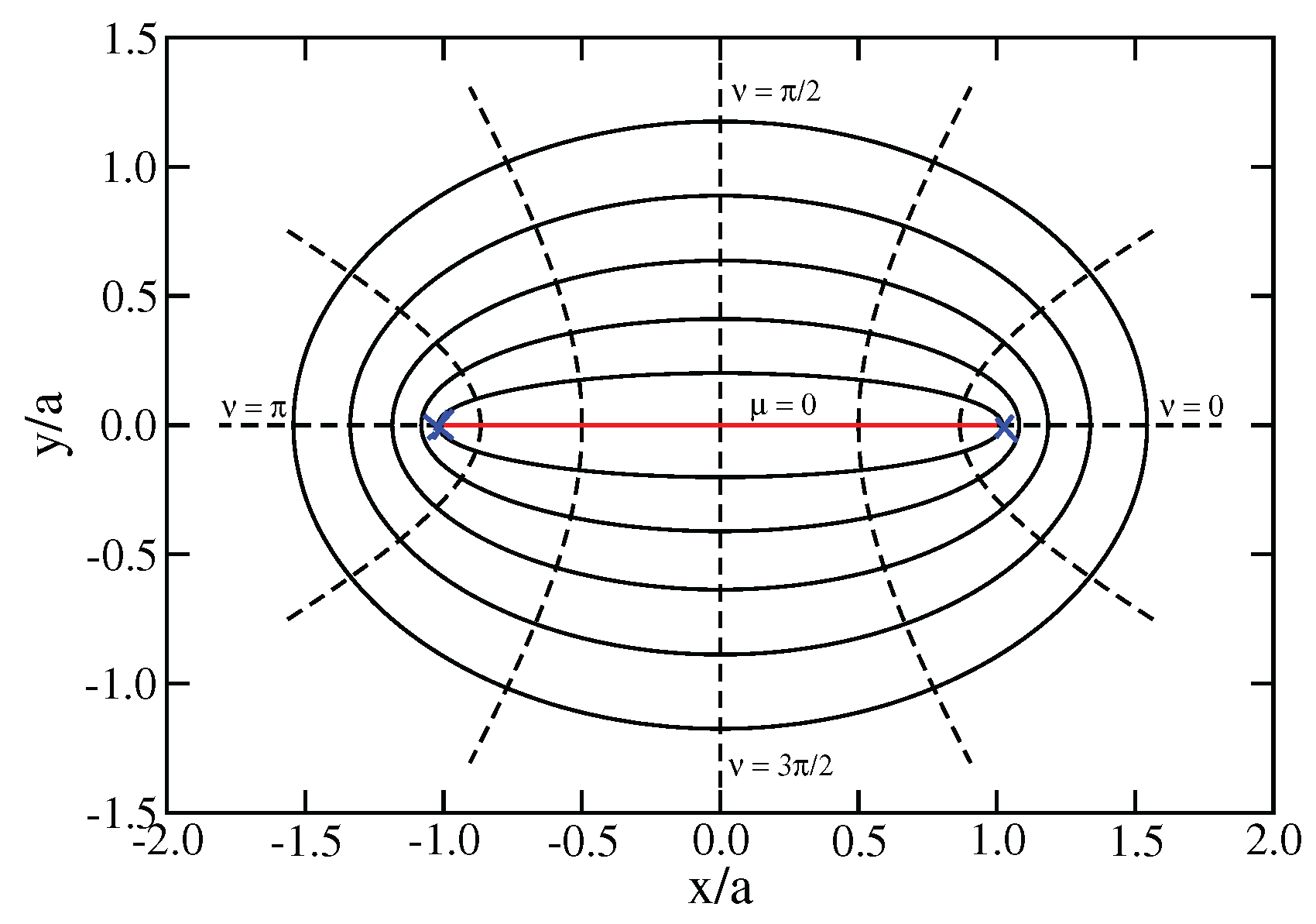
These definitions correspond to ellipses and hyperbolae for constant and , respectively, i.e.
An alternative definition of elliptical coordinates is , where and . The curves of constant are then ellipses and those of constant hyperbolae. Hence, the coordinate belongs to the interval , whereas must be greater than or equal to one. There is a simple geometrical relation of the distances to the foci and . For any point in the plane, the sum of its distances to the foci equals , whereas their difference equals . Thus, the distance to is ), and the distance to is .
According to Abrikosov [32] the radial dependence of an isolated superconducting flux point vortex is approximately . For a distance r much shorter than the coherence length , is linear in r, if the vorticity is one. The sum of the distances to both foci is then and due to the linearity in r, the sum of the pair potential for both vortices is , i.e. it does not depend on and vanishes for .
2.3. BdG Equations in Elliptic Coordinates
The momentum can be expressed in terms of the derivatives with respect to , i.e.
so that
If only one flux quantum is contained in the vortex, we may write . The phase of can be eliminated via a gauge transformation.
The field operators are expanded as
where m is an integer for vorticity one and similarly
The spinor is required to be a single-valued function of , so that
Applying the spinor to we obtain
and
Inserting and the Taylor expansion of [Equation (10)] the differential equation yields
where denotes and , with being . Here we have incorporated the subindex n into the field operator . It is easy to verify that for . Only plays a relevant role and the subindex n can be suppressed. Below we denote the components of the spinor as with , where the index j contains the spin (up or down) and annihilation and creation symbols. The -dependence of is , where and are Pauli matrices for the spin and particle/hole sectors, respectively.
The matrix equation reduces to four linearly coupled differential equations, in which the dependence cancels out and the solution is single valued,
Defining , , , and , the equations are dimensionless and have the following form
These equations are formally similar to those of a single pinned point vortex [7,8,12] described by polar coordinates. However is not the radial coordinate so that the meaning of these equations in Cartesian coordinates is substantially different. and are both angular coordinates.
2.4. Majorana State
The Majorana bound state has zero energy and corresponds to . It is easily verified that the solution of Equations (19)–(22) is given by
where are Bessel functions of integer order, C is a normalization constant and is given by
Note that the definition of is different from the corresponding expression for a point vortex in polar coordinates. [12,13] The Majorana wave function is
A Majorana state is self-adjoint and should satisfy . The adjoint of the first term in (25) yields the third term and the adjoint of the second term yields the fourth term.
3. Results
3.1. Excitation Energies
The solution of the BdG equations for the general case is outlined in the Appendix, where we have shown that the wave functions of the fermion excited states consist of two factors,
one being a Bessel function and the second one determines the exponential decay of the wave function. The latter, , is a function of the superconducting order parameter. The energies are equally spaced and depend on the function , Equation (24). Since the superconducting gap is a linear function of distance with slope , where is the coherence length, is easily evaluated yielding
As shown in Figure 2 the function is approximately parabolic and decreases with increasing the distance between the foci .
The energies are given by Equation (A34), where the matching point at the lower integration limit can be approximated by . It needs to be verified that as a function of the upper integration limit the value of the converges. This convergence is shown in Figure 3 for the same values of as in Figure 2. The energy saturates into plateaus with increasing . The gap between consecutive excited states decreases with increasing . For given the excited states are equidistant, i.e. , where corresponds to the Majorana state.
3.2. Local Density of Bound States
The one-particle Green’s function for spin-component is given by the wave functions and energy eigenvalues [37]
where u and v correspond to the functions , i.e. the wave functions for particles and holes. The local density of states (LDOS) for spin projection is given by the imaginary part of the Green’s function for
At finite temperature the -function is substituted by minus the derivative of the Fermi function, and hence the peaks broaden with increasing temperature. [17]
The LDOS for our model with Rashba interaction is proportional to (up to a normalization constant for the spinor)
The above expressions are formally identical to the ones for a point vortex with two important differences, namely, the function is not the same and in the present case is not the distance to the origin of the vortex, but a function of elliptical coordinates. The zero energy Majorana state corresponds to and . The total LDOS () is invariant under the transformation , i.e. , and , i.e. the simultaneous interchange of the particle and hole amplitudes. It is interesting to notice that as for a point vortex the LDOS is not particle-hole symmetric.
To understand the lack of particle-hole symmetry we consider Equations (12) and (13) and arguments similar to Ref. [12]. For down-spin electrons the effective angular momentum is m, while for up-spin electrons it is . On the other hand, for down-spin holes it is still m, but for up-spin holes it is . As a consequence of the difference between electrons and holes with up-spin, the particle-hole symmetry is broken. The origin of this asymmetry is the Rashba spin-orbit interaction. Hence, the LDOS is asymmetric as a function of .
The LDOS is measurable via scanning tunneling microscopy (STM) by fine-tuning the energy at a distance from the core of the linear vortex, parametrized by .
The LDOS as a function of energy in units of the gap is shown in Figure 4 for three values of . The intensity of the peaks depends on (i) the Bessel functions, (ii) the exponential decay due to , and (iii) on the separation of the two foci, . The LDOS also decreases rapidly as a function of temperature. The Majorana state () has always the same intensity as the peak. In general, the LDOS is symmetric about . For and zero distance between the foci, , i.e. for a simple point vortex, there are only two peaks, namely and 1, as a consequence of the Bessel functions, , which are zero as for . More peaks appear at finite and/or finite , but for larger or the intensity does not necessarily decrease monotonically with m as a consequence of the oscillations of the Bessel functions.
For example in Figure 4c for and the peak has higher intensity than the state. This can be understood with the plot of the intensities as a function of displayed in Figure 5. For the and 1 peaks have smaller intensity than the and 3 peaks. But for larger energies the intensity of the peaks decreases rapidly. For the main maxima of the LDOS form concentric circles about the center of the core with their radius increasing with m. For , on the other hand, the main maxima of the LDOS follow ellipses.
The intensities of the peaks are shown in Figure 5 as a function of and for two values of . Note that . The peaks are denoted by two consecutive m values indicating, e.g. ; the curve is black, the curve is red, the curve is green and the curve is blue. As already mentioned, the oscillations arise from the Bessel functions.
3.3. Spin Polarization
Of interest is also the spin-polarization of the peaks in the LDOS. For (point vortex) and the Majorana state is purely a down-spin peak. With increasing a and a growing up-spin component arises. On the other hand, the peak is predominantly up-spin, with growing down-spin components as a and increase. This pattern is shown in Figure 6 and can be expressed as with in units of the excitation energy . Note that is a symmetric function of , while is even about , and the sum of and yields the total LDOS, , which is symmetric about .
3.4. Orbits in Cartesian Coordinates
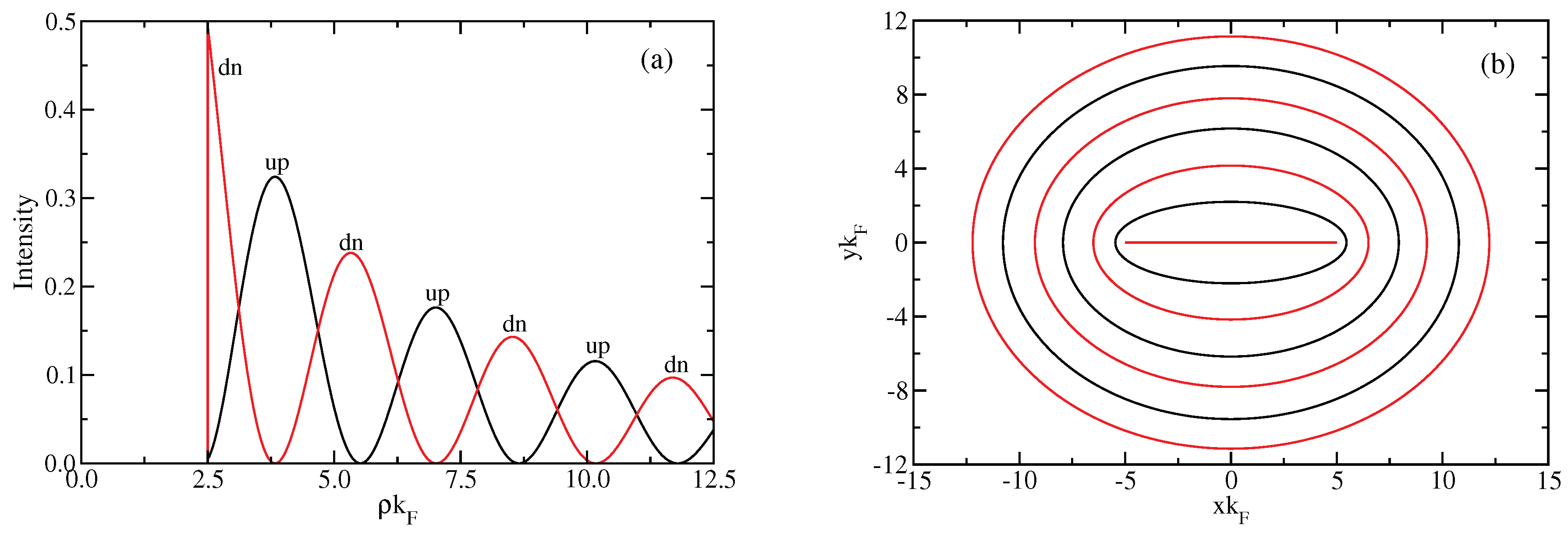
So far we investigated the solution of the bound states in terms of the natural elliptic coordinates, and . These variables do not correspond to the real space Cartesian coordinates x and y, defined by the elliptic coordinates Equation (4). We now consider the zero-energy Majorana state, which is given by the zero-order (down-spin density) and first-order (up-spin density) Bessel functions. The oscillations of the Bessel functions give rise to maxima and minima, which are shown in Figure 7a as a function of for . Here down-spin maxima are displayed in red and up-spin maxima in black. Note that solutions only exist for . As a function of the down-spin and up-spin maxima alternate and are approximately equally spaced.
Equation (4) transforms circular solution (natural coordinated for this problem) into elliptical real space coordinates. Note that for the real space pattern is a horizontal segment between and a, which corresponds to a vanishing superconducting gap. The order parameter grows linearly away from this segment. The down- and up-spin maxima ellipses alternate and grow with increasing (see Figure 7b).
4. Concluding Remarks
We investigated the bound states in the vortex core of a line-shaped cut of length in a two-dimensional topological superconductor with Rashba interaction by solving the BdG equations following the analytic method outlined by Caroli et al. [23] The electron gas corresponds to the surface states of a 3D TI with proximity induced superconductivity from a nearby s wave superconductor. [3,6,7,9] This way the model is reduced to an effective 2D superconductor with a linear pinning defect between the two foci. The superconductor is gapless along the linear defect. The strong spin-orbit interaction locks the momentum and the spin perpendicularly. The characteristic energy scale for the spacing of the energy levels in the vortex is proportional to .
The calculation yields a string of fermion bound states with energy , , and a bound state with Majorana statistics for and . In the present case the pinning defect has a linear shape of length . The results are similar to those of a point defect studied previously, [12,13,15] except that instead of concentric circles the curves of constant energy now are ellipses. The gapless region in the present case is the segment of length , while for the point defect the gap only vanishes at the singular point. The analytical expressions for the wave functions, consist of products of a Bessel function and an exponential decay, , as function of the parameter (which for an ellipse is different than the radius of the circle). Given the wave functions we obtained an analytic expression of the LDOS for the bound states. This quantity is experimentally accessible via STM. [26]
We investigated the LDOS as a function of external frequency, temperature, the distance from the center of the vortex and the length between the foci. The intensity of the peaks in the LDOS rapidly decreases with temperature due to the smearing of the Fermi function. It is interesting to notice that the particle-hole symmetry is broken in the LDOS as a consequence of the spin-orbit coupling. This can be traced to Equation (2). For instance, the Majorana peak is a pure down-spin state at the core of a point vortex, but becomes partially polarized away from the center and for finite a.
The main difference between the ordinary superconductor and the topological superconducting gas is the spin-locking. In the latter in a closed path the spin is forced to follow the momentum giving rise to a non-trivial Berry phase of 1/2. This converts the half-integer quantum numbers into integer ones and opens the possibility to the existence of a Majorana fermion.
The experimental search for zero-energy modes was successful in two systems, namely, heterostructures of Bi2Te3/NbSe2[25,33,34] and monolayers of the high-temperature superconductor FeTe0.55Se0.45 on SrTiO3(0011).[26,27,28,35] Both systems have the advantage of relatively large superconducting transition temperatures. A zero-energy mode, however does not imply a Majorana state, since it may as well originate from a magnetic impurity or an Andreev reflection. The verification that a zero-energy mode corresponds to a Majorana state requiresbraiding, i.e. exchanging the positions of two Majorana zero modes.
Data Availability Statement
The data that support the findings of this article are not publicly available. The data are available from the author upon reasonable request.
Appendix A. Solution of Bogoliubov-de Gennes Equations
The method of CdeGM [12,23,24] consists of solving the equations (i) for small and (ii) for larger , but distances smaller than the coherence length . The solutions for the two regimes are then matched at an intermediate distance, . If the matching condition is independent of , the solution is valid for the entire vortex region. This condition also determines the bound state energies inside the vortex.
Appendix A.1. Second Order Differential Equations
We first convert the first order differential equations, Equations (19)–(22), into second order differential equations.[12,13,23,24] For instance, we express from Equation (19) and insert it into Equation (20) and similar substitutions for , and . Defining and for particles and holes, respectively, we obtain
Appendix A.2. Solution for <
Since , where is the coherence length, for we may neglect in the core of the vortex. The equations for are then of the integer Bessel function type
For , the solutions for are then
The constants are not all independent. Inserting the solutions into the first order differential equations (still with ) we obtain and . and are independent for , but are coupled for , so that and (see Appendix 4).
Appendix A.3. Solution for >
In this case plays an important role. An Ansatz for a solution of the second order differential equations is in terms of a Hankel function of the first kind times an envelope function [37]
where and the are constants. We postulate , where the normalization constant B is equated to one for simplicity. The relative phases of the are the same as in Equations (A9)-(A12). This choice of is verified below where the wave function for is matched to the one for .
It is convenient to rewrite Equation (A1) as
and similarly for the remaining three equations, Equations (A2)-(A4). The first line corresponds to the differential equation of the Hankel function. Inserting Equation (A13) into Equation (A14), dividing by and using the asymptotic expansion of the Hankel function for large argument,
we obtain the following differential equations for the functions :
These equations are solved iteratively. To zeroth order we keep the dominant terms,
The remaining terms are first order terms and will be treated perturbatively. The solution of Equation (A20) is of the form
where has been defined previously in Equation (24) and C is a unitary constant to be determined later.
The equations for the first order terms in Equations (A16)-(A19) are
Inserting the zero-order solutions, Equation (A21), into Equation (A22) and considering the Ansatz , , and , we obtain
where terms of the order and vanish identically. All terms are proportional to , so that this factor cancels out. The differential equations then take the following form
which can be decoupled by taking linear combinations,
The above equations can be integrated
We are only interested in leading and next-leading terms and will disregard higher order terms. Small parameters are , and , so that the term of Equation (A28) and the last term of Equation (A29) can be neglected.
The remaining two integrals can be integrated by parts:
and
The function equals zero at the matching point (see Appendix 4) and defines the bound state energies.
It is now straightforward to solve Equations (A26)-(A29) for
This corresponds to the leading and next-leading solution for the wave function for large argument.
Appendix A.4. Matching of Wave Functions
The next step consists in matching the solution for the wave function for small and large at an intermediate value from the core of the vortex. The wave function is determined uniquely if this matching is independent of . This condition on also implies that and consequently the energy for the bound state is given by
The excited states are then equally spaced energy levels.
The solutions for are given by , where the coefficients are defined just after (Equation (A13)). The functions were calculated consistently to first order of perturbation and can be written as an exponential, i.e. . This expression remains correct to first order. For the solutions are Equations (A9)–(A12), which have to be matched at following a procedure similar to Refs. [12] and [23]. To match the wave functions we use the asymptotic expansions for the Bessel and Hankel functions. To simplify we only explicitly work out the matching for the function ; the remaining three functions follow similarly.
Appendix A.5. Wave Functions for Excited States
Approximate expressions to leading order for the amplitudes of the wave functions for the excited bound states, , are given by
and the energy wave function with energy is then
While for the wave function corresponds to a Majorana state (), for it represents an ordinary fermion wave function (not self-adjoint). Note that for , , so that there is an additional minus sign, making the difference between a Majorana and ordinary fermion.
References
- Beenakker, C.W.J. Search for Majorana Fermions in Superconductors. Annu. Rev. Condens. Matter Phys. (2013), 4, 113. [Google Scholar] [CrossRef]
- Kitaev, A.Yu. Unpaired Majorana fermions in quantum wires. Physics-Uspekhi (2001), 44, 131. [Google Scholar] [CrossRef]
- Fu, L.; Kane, C.L. Superconducting Proximity Effect and Majorana Fermions at the Surface of a Topological Insulator. Phys. Rev. Lett. (2010), 100, 096407. [Google Scholar] [CrossRef]
- Fu, L.; Kane, C.L. Probing Neutral Majorana Fermion Edge Modes with Charge Transport. Phys. Rev. Lett. (2009), 102, 216403. [Google Scholar] [CrossRef]
- Sau, J.D.; Lutchyn, R.M.; Tewari, S.; Das Sarma, S. Robustness of Majorana fermions in proximity-induced superconductors. Phys. Rev. B (2010), 82, 094522. [Google Scholar] [CrossRef]
- Chiu, Ch.-K.; Cole, W.S.; Das Sarma, S. Induced spectral gap and pairing correlations from superconducting proximity effect. Phys. Rev. B (2016), 94, 125304. [Google Scholar] [CrossRef]
- Rakhmanov, A.L.; Rozhkov, A.V.; Nori, F. Majorana fermions in pinned vortices. Phys. Rev. B (2011), 84, 075141. [Google Scholar] [CrossRef]
- Akzyanov, R.S.; Rozhkov, A.V.; Rakhmanov, A.L.; Nori, F. Tunneling spectrum of a pinned vortex with a robust Majorana state. Phys. Rev. B (2014), 89, 085409. [Google Scholar] [CrossRef]
- Sau, J.D.; Lutchyn, R.M.; Tewari, S.; Das Sarma, S. A generic new platform for topological quantum computation using semiconductor heterostructures. Phys. Rev. Lett. (2010), 104, 040502. [Google Scholar] [CrossRef] [PubMed]
- Mao; Li; Zhang, Ch. Robustness of Majorana modes and minigaps in a spin-orbit-coupled semiconductor-superconductor heterostructure. Phys. Rev. B (2010), 82, 174506. [Google Scholar] [CrossRef]
- Berthod, C. Vorticity and vortex-core states in type-II superconductors. Phys. Rev. B (2005), 71, 134513. [Google Scholar] [CrossRef]
- Deng, H.; Bonesteel, N.; Schlottmann, P. Bound fermion states in pinned vortices in the surface states of a superconducting topological insulator. J. Phys.: Condens. Matter (2021), 33, 035604. [Google Scholar] [CrossRef]
- Schlottmann, P. Local density of states in a vortex at the surface of a topological insulator in a magnetic field. Eur. Phys. J. B (2021), 94, 119. [Google Scholar] [CrossRef]
- Beenakker, C.W.J. Random-matrix theory of Majorana fermions and topological superconductors. Rev. Mod. Phys. (2015), 87, 1037. [Google Scholar] [CrossRef]
- Ziesen, A.; F. Hassler, F. Low-energy in-gap states of vortices in superconductor-semiconductor heterostructures. J. Phys.: Condens. Matter (2021), 33, 294001. [Google Scholar] [CrossRef] [PubMed]
- Ioselevich, P.A.; Ostrovsky, P.M.; Feigel’man, M.V. Majorana state on the surface of a disordered three-dimensional topological insulator. Phys. Rev. B (2012), 86, 035441. [Google Scholar] [CrossRef]
- Suzuki, S.-I.; Kawaguchi, Y.; Tanaka, Y. Local density of states in two-dimensional topological superconductors under a magnetic field: Signature of an exterior Majorana bound state. Phys. Rev. B (2018), 97, 144516. [Google Scholar] [CrossRef]
- Akzyanov, R.S.; Rakhmanov, A.L.; Rozhkov, A.V.; Nori, F. Majorana fermions at the edge of superconducting islands. Phys. Rev. B (2015), 92, 075432. [Google Scholar] [CrossRef]
- Akzyanov, R.S.; Rakhmanov, A.L.; Rozhkov, A.V.; Nori, F. Tunable Majorana fermion from Landau quantization in 2D topological superconductors. Phys. Rev. B (2016), 94, 125428. [Google Scholar] [CrossRef]
- Chamon, C.; Jackiw, R.; Nishida, Y.; Pi, S.-Y.; Santos, L. Quantizing Majorana fermions in a superconductor. Phys. Rev. B (2010), 81, 224515. [Google Scholar] [CrossRef]
- Khaymovich, I.M.; Kopnin, N.B.; Mel’nikov, A.S.; Shereshevskii, I.A. Vortex core states in superconducting graphene. Phys. Rev. B (2009), 79, 224506. [Google Scholar] [CrossRef]
- Beenakker, C.W.J. Specular Andreev reflection in graphene. Phys. Rev. Lett. (2006), 97, 067007. [Google Scholar] [CrossRef] [PubMed]
- Caroli, C.; De Gennes, P.G.; Matricon, J. Bound Fermion states on a vortex line in a type II superconductor. Phys. Lett. (1964), 9, 307. [Google Scholar] [CrossRef]
- Caroli, C.; Matricon, J. Excitations électroniques dans les supraconducteurs purs de 2ème espèce. Phys. kondens. Materie (1965), 3, 380. [Google Scholar] [CrossRef]
- Sun, H.-H.; Zhang, K.-W.; Hu, L.-H.; Li, Ch.; Wang, G.-Y.; Ma, H.-Y.; Xu, Z.-A.; Gao, Ch.-L.; Guan, D.-D.; Li, Y.-Y.; Liu, C.; Qian, D.; Zhou, Yi; Fu, L.; Li, Sh.-Ch.; Zhang, Fu-Ch.; Jia, J.-F. Majorana Zero Mode Detected with Spin Selective Andreev Reflection in the Vortex of a Topological Superconductor. Phys. Rev. Lett. (2016), 116, 257003. [Google Scholar] [CrossRef]
- Wang, D.; Kong, L.; Fan, P.; Chen, H.; Zhu, Sh.; Liu, W.; Cao, Lu; Sun, Y.; Du, Sh.; Schneeloch, J.; Zhong, R.; Gu, G.; Fu, L.; Ding, H.; Gao, H.-J. Evidence for Majorana bound states in an iron-based superconductor. Science (2018), 362, 333. [Google Scholar] [CrossRef]
- Machida, T.; Sun, Y.; Pyon, S.; Takeda, S.; Kohsaka, Y.; Hanaguri, T.; Sasagawa, T.; Tamegai, T. Zero-energy vortex bound state in the superconducting topological surface state of Fe(Se,Te). Nat. Matter (2019), 18, 811. [Google Scholar] [CrossRef] [PubMed]
- Chen, C.; Jiang, K.; Zhang, Y.; Liu, C.; Liu, Y.; Wang, Z.; Wang, J. Atomic line defects and zero-energy end states in monolayer Fe(Te,Se) high-temperature superconductors. Nat. Phys. (2020), 16, 536. [Google Scholar] [CrossRef]
- Zyuzin, A.; Alidoust, M.; Loss, D. Josephson junction through a disordered topological insulator with helical magnetization. Phys. Rev. B (2016), 93, 214502. [Google Scholar] [CrossRef]
- Bobkova, I.V.; Bobkov, A.M. Electrically controllable spin filtering based on superconducting helical states. Phys. Rev. B (2017), 96, 224505. [Google Scholar] [CrossRef]
- https://en.wikipedia.org/wiki/Elliptic-Coordinate-System.
- Abrikosov, A.A. On the magnetic properties of superconductors of the second group. Soviet Phys. JETP (1957), 5, 1174. [Google Scholar]
- Xu, J.-P.; Wang, M.-X.; Liu, Z. L.; Ge, J.-F.; Yang, X.; Liu, C.; An Xu, Z.; Guan, D.; Gao, Ch. L.; Qian, D.; Liu, Y.; Wang, Q.-H.; Zhang, Fu-Ch.; Xue, Qi-K.; Jia, J.-F. Experimental Detection of a Majorana Mode in the core of a Magnetic Vortex inside a Topological Insulator-Superconductor Bi2Te3/NbSe2 Heterostructure. Phys. Rev. Lett. (2015), 114, 017001. [Google Scholar] [CrossRef]
- Sun, H.-H.; Jia, J.-F. Majorana zero mode in the vortex of an artificial topological superconductor. Science China: Physics, Mechanics & Astronomy (2017), 60, 057401. [Google Scholar]
- Kong, L.; Zhu, S.; Papaj, M.; Chen, H.; Cao, Lu; Isobe, H.; Xing, Y.; Liu, W.; Wang, D.; Fan, P.; Sun, Y.; Du, S.; Schneeloch, J.; Zhong, R.; Gu; Fu, G.L.; Gao, H.-J.; Ding, H. Half-integer level shift of vortex bound states in an iron-based superconductor. Nat. Phys. (2019), 15, 1181. [Google Scholar] [CrossRef]
- Schlottmann, P. In-gap states of vortices at the surface of a topological insulator. Physica C: Superconductivity and its Applications (2022), 596, 1354047. [Google Scholar] [CrossRef]
- Bardeen, J.; Kümmel, R.; Jacobs, A.E.; Tewordt, L. Structure of Vortex Lines in Pure Superconductors. Phys. Rev. (1969), 187, 556. [Google Scholar] [CrossRef]
Figure 2.
(color online) The function normalized to for five values of , namely 1 (black), 5 (red), 10 (green), 15 (blue), and 20 (magenta). At large distances the wave function falls off faster with increasing K. is approximately a parabolic function.
Figure 2.
(color online) The function normalized to for five values of , namely 1 (black), 5 (red), 10 (green), 15 (blue), and 20 (magenta). At large distances the wave function falls off faster with increasing K. is approximately a parabolic function.
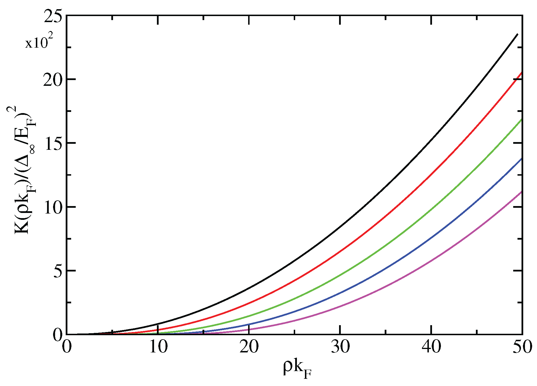
Figure 3.
(color online) First excited state energy : In Equation (A34) we set and replace the upper integration limit ∞ by . For large , saturates yielding the excited energy. Five values of are considered, 1 (black), 5 (red), 10 (green), 15 (blue), and 20 (magenta), where is the distance between the foci. The energy of the excited state decreases with increasing .
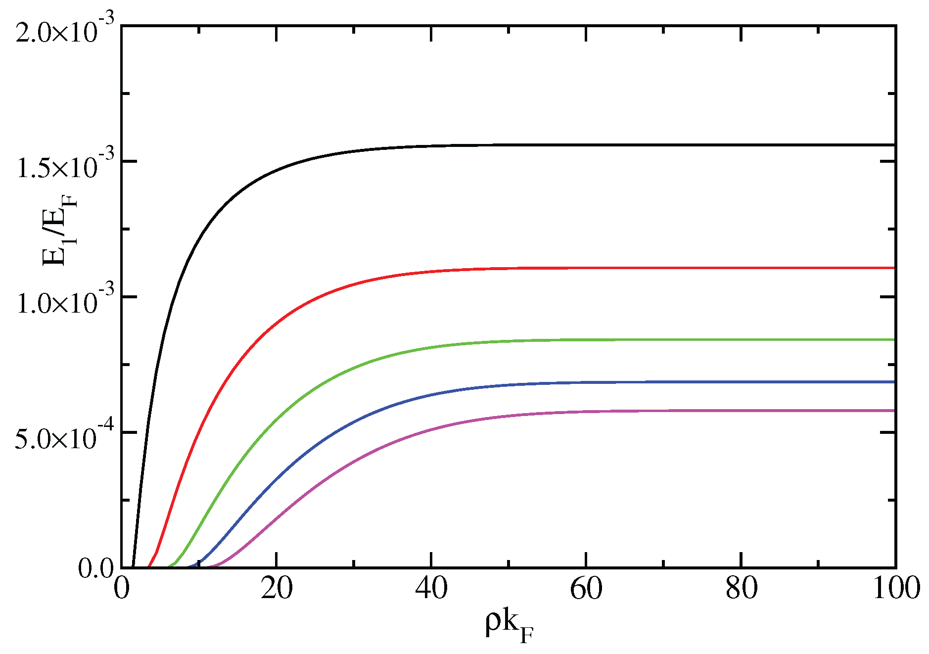
Figure 4.
(color online) LDOS of the bound states in the linear vortex of length as a function of energy for and three values of , namely, 0.5 in panel (a), 1.0 in panel (b) and 2.0 in panel (c). The three curves in each panel represent different temperatures: (black), (red) and (blue). In the limit the peaks are delta-functions. The function K is given by Equation (26). All energies are given in units of , i.e. the spacing between excitations, and the LDOS is in arbitrary units but the same units for all three panels. Note that the LDOS is not particle-hole symmetric. Since more than two peaks have nonzero spectral weight.
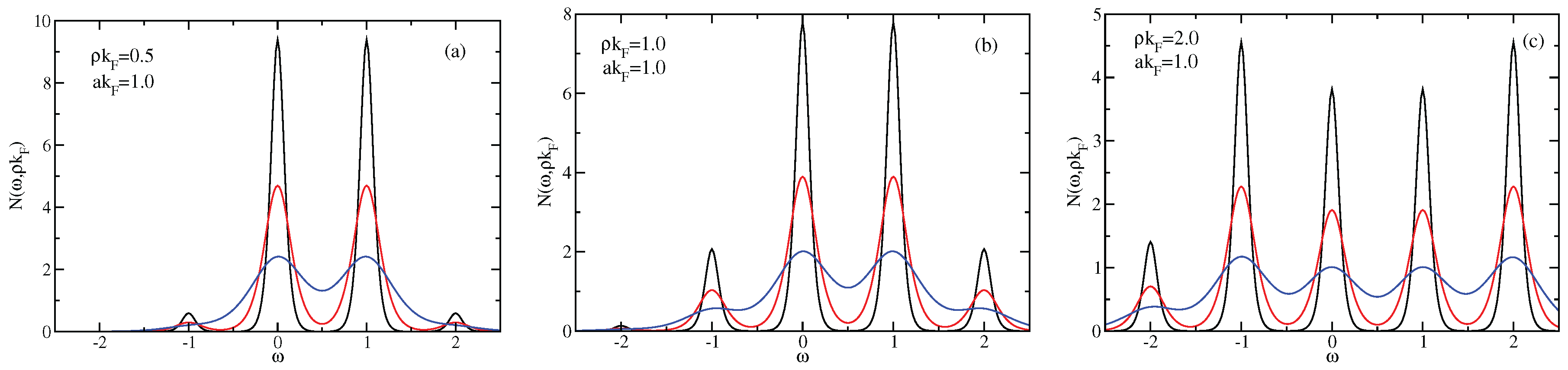
Figure 5.
(color online) Intensities of the peaks as a function of for several m. In general the intensity decreases with , m and , but not necessarily monotonically. for panel (a) and for panel (b). Note that . The colors of the curves are: (black), (red), (green) and (blue).
Figure 5.
(color online) Intensities of the peaks as a function of for several m. In general the intensity decreases with , m and , but not necessarily monotonically. for panel (a) and for panel (b). Note that . The colors of the curves are: (black), (red), (green) and (blue).
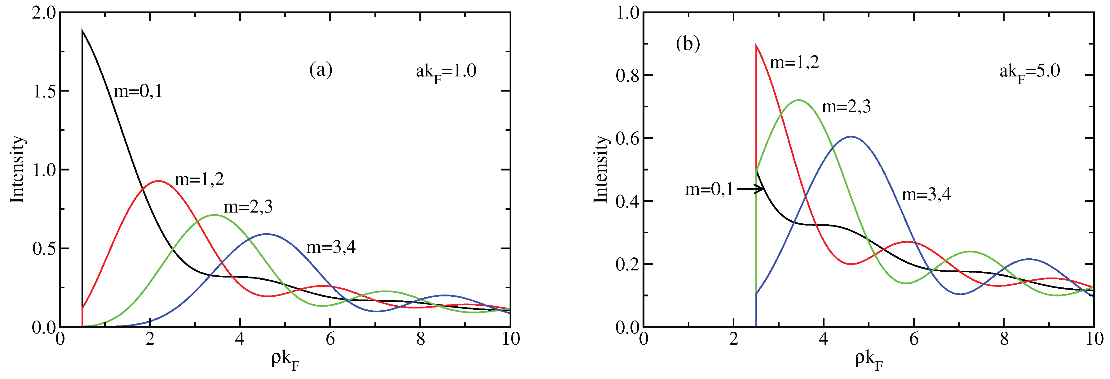
Figure 6.
(color online) Spin-polarized LDOS in arbitrary units of the bound states in the linear vortex as a function of energy for and , (a) up-spin and (b) down-spin. Note that the LDOS for down-spin is symmetric, while the LDOS for up-spin is asymmetric, shifted by one unit towards positive energies. The three curves in each panel represent different temperatures: (black), (red) and (blue). The intensity decreases rapidly with the temperature.
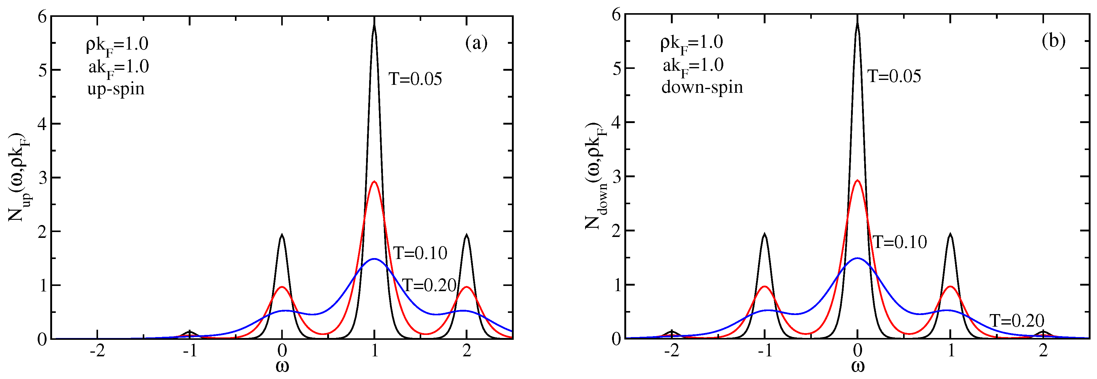
Figure 7.
(color online) (a) Spin-polarized maxima of the LDOS in arbitrary units for the Majorana state in the linear vortex as a function of for . Up- (black) and down-spin (red) maxima alternate and decrease monotonically with . (b) The orbital pattern are circles with growing radius for coordinates and , while they are ellipses for real space coordinates, x and y. The red straight line represents the gapless region.
Disclaimer/Publisher’s Note: The statements, opinions and data contained in all publications are solely those of the individual author(s) and contributor(s) and not of MDPI and/or the editor(s). MDPI and/or the editor(s) disclaim responsibility for any injury to people or property resulting from any ideas, methods, instructions or products referred to in the content. |
© 2025 by the authors. Licensee MDPI, Basel, Switzerland. This article is an open access article distributed under the terms and conditions of the Creative Commons Attribution (CC BY) license (http://creativecommons.org/licenses/by/4.0/).
Copyright: This open access article is published under a Creative Commons CC BY 4.0 license, which permit the free download, distribution, and reuse, provided that the author and preprint are cited in any reuse.


