From Quantum to Reality. Gravity-Induced Quantum Decoherence, Arrow of Time, Matter Self-Assembling, Life, Intelligence, Consciousness, and Free Will. Part One: The Emergence of Classical Reality

1. Introduction

In this work, the authors seek to outline the common thread that leads to the emergence of classical reality, where life manifests, grounded in the physical principles of spacetime.

While gravity, quantum mechanics, classical mechanics, and far-from-equilibrium order generation are well-established disciplines, they remain disconnected from one another, and a unified framework of the universe evolution and generation of macroscopic reality is still lacking.

In this context, the paper aims to explores how the gravitational background noise of spacetime interacts with quantum mechanics, giving rise to the macroscopic classical world. The emergence of classical reality, through the gravitationally induced stochastic quantum mechanics, reveals details about long-standing problems including the EPR paradox, quantum–classical coexistence, the time's flow in 4-D reality, the order generation and matter self-assembly.

In the absence of these critical connections, understanding the emergence of real life from a physical perspective—one of the great challenges of modern science—is destined to remain unresolved.

2. Quantum Properties of Spacetime with Fluctuating Gravitational Background

At the quantum level, spacetime undergoes stochastic fluctuations driven by GBN, relics of the Big Bang, and the relativistic dynamics of massive bodies. In what follows, we will demonstrate that these fluctuations generate curvature wrinkles that disturb quantum systems, ultimately leading to decoherence and the transition to classical behavior.

The non-locality of quantum mechanics, as exemplified by the EPR paradox, presents significant challenges in reconciling it with the locality of relativistic spacetime [1,2]. The stochastic quantum hydrodynamic approach incorporates these spacetime fluctuations into the quantum potential, effectively suppressing long-range quantum coherence. This mechanism enables the transition to classical mechanics without requiring an external environment or ad hoc assumptions, thus addressing the fundamental issues of the quantum-to-classical transition and wavefunction collapse.

Recent advancements in decoherence theory confirm that interactions with fluctuations play a crucial role in localizing quantum states [3,4,5,6]. The proposed SQHM builds on these insights, treating spacetime itself as a self-fluctuating system—devoid of an external environment—that gradually loses quantum coherence on scales both larger than the de Broglie wavelength and the theory-defined action distance of the quantum potential [7].

2.1. The Stochastic Quantum Hydrodynamic Model

The Madelung quantum hydrodynamic representation transforms the Schrodinger equation

$$-i\hslash {\partial }_t\psi =\left({\displaystyle \frac{{\hslash }^2}{2m}}{\partial }_i{\partial }_i-V_{(q)}\right)\psi$$

(1)

for the complex wave function $\psi =\left|\psi \right|{\mathrm{e}}^{-{\displaystyle \frac{iS}{\hslash }}}$, into two equations of real variable [8,9,10]: the conservation equation for the mass density $n_{(q,t)}=|\psi {|}^2$

$${\partial }_t{n}_{(q,t)}+{\partial }_i(n_{(q,t)}{\dot{q}}_i)=0$$

(2)

and the motion equation for the momentum $m{\dot{q}}_i=p_i={\partial }_i{S}_{(q,t)}$,

$${\ddot{q}}_i=-{\displaystyle \frac{1}{m}}{\partial }_i\left(V_{(q)}+V_{q{u}_{(n)}}\right)$$

(3)

where$S_{(q,t)}=-{\displaystyle \frac{\hslash }{2}}\ln {\displaystyle \frac{\psi }{\psi *}}$and where

$$V_{qu}=-{\displaystyle \frac{{\hslash }^2}{2m}}{\displaystyle \frac{1}{\left|\psi \right|}}{\partial }_i{\partial }_i\left|\psi \right|$$

(4)

Following the hypothesis that considers the GBN as a source of quantum decoherence [11] and by introducing it into Madelung quantum hydrodynamics, equation (1-4) yields a generalized stochastic quantum model capable of describing wavefunction collapse dynamics and the measurement process, leading to a fully self-consistent generalized quantum theory [12,13].

To incorporate the presence of the GBN into equations (1–4), we must account for how it perturbs the quantum physical system. The first contribution arises from the energy content of the GBN, which, according to the principle of mass-energy equivalence in General Relativity, can be represented as a locally fluctuating mass density. As shown in [7,13], this effect of the GBN can be described by the following assumptions:

• The mass density of GBN is described by its wavefunction ${\psi }_{gbn}$with density$|{\psi }_{gbn}{|}^2$;
• The associated energy density $E$of GBN is proportional to $|{\psi }_{gbn}{|}^2$;
• The associated mass $m_{gbn}$of GBN is defined by the identity $E=m_{gbn}{c}^2|{\psi }_{gbn}{|}^2$
• The GBN mass density is approximately assumed to not interact with the mass of the physical system (since the gravitational interaction is sufficiently weak to be disregarded in the Hamiltonian potential $V_{(q)}$in (3)) and the wavefunction of the overall system ${\psi }_{tot}$reads as

  $${\psi }_{tot}\cong \psi {\psi }_{gbn}$$

  (5)

Additionally, given that the energy density $E$ of GBN is quite small, the mass density $m_{gbn}|{\psi }_{gbn}{|}^2$ is presumed to be significantly smaller than the body mass density typically encountered in physical problems. Hence, considering the mass $m_{gbn}$ to be much smaller than the mass of the system, we can assume $m_{tot}=m_{gbn}+m\cong m$ in Equations (3-4).

The second effect of the GBN arises from the gravitational (geometrical) nature of its mass/energy distribution, which induces local variations in the mass density of the physical system. These fluctuations in mass density of the physical system can be understood by noting that gravitational waves are metric perturbations that cause spacetime itself to oscillate. This oscillation leads to contractions and elongations of distances, similar to the effects observed in gravitational wave detections at the LIGO and VIRGO laboratories. As a result, when the wavefunction undergoes such spatial elongations or contractions, the system’s mass density distribution correspondingly decreases or increases. In this way, spatial contractions and elongations influence the quantum potential energy, as it depends on the mass concentration of the physical system.

By introducing the GBN-induced mass density fluctuations into the quantum potential (4), and following the procedure outlined in reference [7,13], Equations (1–4) lead to a system of stochastic quantum differential motion equations.

For systems whose physical size is on the order of the De Broglie wavelength, the resulting quantum-stochastic hydrodynamic equations governing the evolution of the complex field...

$$\psi ={\rho }^{1/2}{\mathrm{e}}^{-{\displaystyle \frac{iS}{\hslash }}}.$$

(6)

, acquire a simpler form and reads [7,13]

$${\ddot{q}}_{j_{(t)}}=-\kappa {\dot{q}}_{j_{(t)}}-{\displaystyle \frac{1}{m}}{\displaystyle \frac{\partial \left(V_{(q)}+V_{q{u}_{(\rho )}}\right)}{\partial q_j}}+\kappa D_{1/2}{\xi }_{(t)}$$

(7)

$$V_{q{u}_{(\rho )}}=-{\displaystyle \frac{{\hslash }^2}{2m}}{\displaystyle \frac{1}{{\rho }^{1/2}}}{\partial }_i{\partial }_i{\rho }^{1/2}$$

(8)

$$m{\dot{q}}_i=p_i={\partial }_i{S}_{(q,t)}=-{\displaystyle \frac{\hslash }{2}}{\partial }_i\left(\ln {\displaystyle \frac{\psi }{\psi *}}\right)$$

(9)

Given the physical length of the system$L$, the diffusion coefficient in (7) can be readjusted as

$$D^{1/2}=\left({\displaystyle \frac{L}{{\lambda }_c}}\right){\left({\gamma }_D{\displaystyle \frac{\hslash }{2m}}\right)}^{1/2}=\sqrt{{\gamma }_D}{\displaystyle \frac{L}{2}}\sqrt{{\displaystyle \frac{kT}{2\hslash }}}$$

(10)

where ${\gamma }_D$ depends by the characteristics of the system [7,13], and

$${\lambda }_c=\sqrt{2}{\displaystyle \frac{\hslash }{{(mkT)}^{1/2}}}$$

(11)

is the De Broglie length defining physical distance below which the quantum coherence is maintained in presence of fluctuations and the friction coefficient $\kappa$is of the form

$$\kappa \cong \alpha {\displaystyle \frac{2kT}{mD}}$$

(12)

where the semiempirical parameter $\alpha$, expressing the ability of the system to dissipate energy, obeys to the condition [7,13]

$${\lim }_{{\displaystyle \frac{L}{{\lambda }_c}}orT\to 0}\alpha =0$$

(13)

Incorporating the time-reversal symmetry of quantum mechanics.

From a general perspective, the solution of the quantum-stochastic hydrodynamic model (SQHM) for $L\gg {\lambda }_c$, encompassing its macroscopic behavior, is not captured by (7-12) because the force fluctuations ${\varpi }_{(q_{\alpha },t)}$induced by the quantum potential, owing to its non-local nature, possess a finite correlation length such that $<{\varpi }_{(q_{\alpha },t)},{\varpi }_{(q_{\beta }+\lambda ,t+\tau )}>=<{\varpi }_{(q_{\alpha })},{\varpi }_{(q_{\beta })}{>}_{(T)} \mathrm{F}(\lambda )\delta (\tau ){\delta }_{\alpha \beta }$, where$F_{(\lambda )}\propto {\displaystyle \frac{1}{{\lambda }_c}}\exp \left[-{\left({\displaystyle \frac{\lambda }{{\lambda }_c}}\right)}^2\right]$ and depend on the spatial point $q_j$ [7,13] . Only for microscopic systems, where $\lambda \ll {\lambda }_c$ and $F_{(\lambda )}\to \propto {\displaystyle \frac{1}{{\lambda }_c}}$, does the force noise become Markovian.

On a given scale $L\ll {\lambda }_c$, the amplitude of fluctuations, denoted by the diffusion coefficient in (10), tends to zero, indicating a form of noise damping induced by the quantum potential that has no counterpart in classical stochastic systems. From the quantum hydrodynamic standpoint, the mass density distribution behaves like an elastic membrane that becomes increasingly resistant to deformation at wavelengths smaller than the De Broglie wavelength, thereby suppressing the manifestation of gravitational background fluctuations (a quantum effect on geometric gravity).

It is straightforward to see that for $T\to 0$ or equivalently ${\lambda }_c\to \infty$, the Madelung quantum deterministic limit, in the form of the quantum hydrodynamic analogy (1-4), is recovered as well as both ${\lim }_{{\displaystyle \frac{L}{{\lambda }_c}}orT\to 0}\psi =\psi$and ${\lim }_{{\displaystyle \frac{L}{{\lambda }_c}}orT\to 0}{\rho }_{(q,t)}=n_{(q,t)}=|\psi {|}^2$.

The conventional quantum mechanics is recovered for null noise (or equivalently for microscopic systems whose physical length is much smaller than the De Broglie length).

Nonetheless, it must be observed that under special conditions such as ${\lim }_{{\displaystyle \frac{L}{{\lambda }_c}}orT\to 0}\alpha =const$, the SQHM leads to the Brownian quantum behavior [7,13].

In the stochastic quantum hydrodynamic representation, the quantum mass density $n_{(q,t)}=|\psi {|}^2$is generalized by the probability mass density (PMD) ${\rho }_{(q,t)}$ determined by the probability transition function $P(x,z|t,0)$ [14] obeying to the Smoluchowski conservation equation [14] for the Marcovian process (7)

$$P(q,p,q_0,p_0|\left(t\text{'}+\tau -t_0\right),t_0)={\displaystyle \underset{-\infty }{\overset{\infty }{\int }}P(q,p,q\text{'},p\text{'}|\tau ,t\text{'})P(q\text{'},p\text{'},q_0,p_0|t\text{'}-t_0,t_0)}{d}^{3}q\text{'}{d}^{3}p\text{'}$$

(14)

, establishing the phase-space mass density conservation

$$N(q,p,t)={\displaystyle \int P(q,p,q\text{'},p\text{'},|t,0)N_{(q\text{'},p\text{'},0)}}{d}^{3}q\text{'}{d}^{3}p\text{'}$$

(15)

that leads to the spacetime mass density distribution ${\rho }_{(q,t)}$ in the

$${\rho }_{(q,t)}={\displaystyle \underset{-\infty }{\overset{+\infty }{\int }}{N}_{(q,p,t)}}{d}^{3}p$$

(16)

In the context of (7-9), $\psi$ does not denote the quantum wavefunction; rather, it represents the generalized quantum-stochastic probability wave that adheres to the limit. $li{m}_{T\to 0}\psi =\psi$

It is worth noting that the SQHM equations (7-9), stemming from the presence of noise curvature wrinkles of spacetime (a form of dark energy), describe a self-fluctuating quantum system where the noise is an intrinsic property of the reference system that is not generated by an environment. An in-depth discussion regarding the property of true randomness or pseudo-randomness of the gravitational background noise is provided in part two of this work.

2.2. Emerging Classical Behavior

When manually nullifying the quantum potential in the equations of motion for quantum hydrodynamics (1-4), the classical equation of motion emerges [9,10]. However, despite the apparent validity of this claim, such an operation is not mathematically sound as it alters the essential characteristics of the quantum hydrodynamic equations. Specifically, this action leads to the elimination of stationary configurations, i.e., quantum eigenstates, as the balancing force of the quantum potential against the Hamiltonian force —which establishes their stationary condition [9,10]—is eliminated. Consequently, even a small quantum potential cannot be disregarded in conventional quantum mechanics that is the zero-noise 'deterministic' limit of the SQHM (7-9).

Conversely, in the stochastic generalization, it is possible to correctly neglect the quantum potential in (7) when its force is much smaller than the force noise $\varpi$ such as, by (7), $\left|{\displaystyle \frac{1}{m}}{\partial }_i{V}_{qu(\rho )}\right|\ll \left|\kappa D^{1/2}{\xi }_{(t)}\right|$that leads to condition

$$\left|{\displaystyle \frac{1}{m}}{\partial }_i{V}_{qu(\rho )}\right|\ll \kappa \left({\displaystyle \frac{L}{{\lambda }_c}}\right){\left({\gamma }_D{\displaystyle \frac{\hslash }{2m}}\right)}^{1/2}=\kappa \left({\displaystyle \frac{L\sqrt{mkT}}{2\hslash }}\right){\left({\gamma }_D{\displaystyle \frac{\hslash }{2m}}\right)}^{1/2}.$$

(17)

and hence, in a coarse-grained description with elemental cell side $\Delta q$, such as

$${\lim }_{q\to \Delta q}\left.\left|{\partial }_i{V}_{qu(\rho )}\right.\right|\ll m\kappa \left({\displaystyle \frac{L}{{\lambda }_c}}\right){\left({\gamma }_D{\displaystyle \frac{\hslash }{2m}}\right)}^{1/2}=m\kappa \sqrt{{\gamma }_D}{\displaystyle \frac{L}{2}}\sqrt{{\displaystyle \frac{kT}{2\hslash }}}$$

(18)

It is worth noting that, despite the noise $\kappa D_{1/2}{\xi }_{(t)}$ having a zero mean, the mean of the fluctuations in the quantum potential, denoted as ${\overline{V}}_{st(\mathrm{n},\mathrm{S})}\cong \kappa S$, is not null. This not-null mean contributes to the frictional dissipative force $-\kappa {\dot{q}}_{(t)}$in equation (7) [7,13]. Consequently, the stochastic sequence of noise inputs disrupts the coherent dynamic evolution of the quantum superposition of states, leading them to frictionally decay to a stationary mass density distribution with ${\dot{q}}_{(t)}=0$. Moreover, by observing that the stochastic force noise

$$\kappa \left({\displaystyle \frac{L}{{\lambda }_c}}\right){\left({\gamma }_D{\displaystyle \frac{\hslash }{2m}}\right)}^{1/2}{\xi }_{(t)}$$

(19)

grows with the size of the system, for macroscopic systems (${\displaystyle \frac{L}{{\lambda }_c}}\to \infty$), condition (17) can be satisfied if

$${\lim }_{{\displaystyle \frac{q}{{\lambda }_c}}\to {\displaystyle \frac{L}{{\lambda }_c}}=\infty }\left|\left.{\displaystyle \frac{1}{m}}{\partial }_i{V}_{qu({\mathrm{n}}_{(q)})}\right|\right.<\infty$$

(20)

Since systems obeying (20) may exhibit a rather extended meso-scale in the transition between quantum to classical behavior, a more stringent requirement such as:

$${\lim }_{{\displaystyle \frac{q}{{\lambda }_c}}\to \infty }\left|\left.{\displaystyle \frac{1}{m}}{\partial }_i{V}_{qu({\rho }_{(q)})}\right|\right.={\lim }_{{\displaystyle \frac{q}{{\lambda }_c}}\to \infty }{\displaystyle \frac{1}{m}}\sqrt{{\partial }_i{V}_{qu({\rho }_{(q)})}{\partial }_i{V}_{qu({\rho }_{(q)})}}=0$$

(21)

can be imposed in cases where the transition from the quantum to classical regime is well-defined and the macroscopic behavior is completely free from non-local quantum potential interaction.

Recognizing that since for linear systems it holds

$${\lim }_{q\to \infty }{V}_{qu(q)}\propto q^2$$

(22)

we readily can observe that these systems are incapable of generating macroscopic classical phases. Generally speaking, as the Hamiltonian potential strengthens, the wave function localization increases and the quantum potential behavior at infinity becomes more prominent.

In fact, by considering the mass density

$$|\psi {|}^2\propto \exp \left[-P^k(t)\right]$$

(23)

where $P^k(t)$ is polynomial of order $k$, it becomes evident that a vanishing quantum potential interaction at infinity is achieved if and only if $k<{\displaystyle \frac{3}{2}}$.

On the other hand, for instance, for gas phases with particles that interact by the Lennard-Jones potential, whose long-distance wave function reads [15]

$${\lim }_{r\to \infty }\left|\psi \right|\propto a^{-1/2}{\displaystyle \frac{1}{r}}$$

(24)

the quantum potential that reads

$${\lim }_{r\to \infty }{V}_{qu(\rho )}\cong {\lim }_{q\to \infty }{\displaystyle \frac{{\hslash }^2}{2m}}{\displaystyle \frac{1}{\left|\psi \right|}}{\partial }_r{\partial }_r\left|\psi \right|={\displaystyle \frac{1}{r^2}}={\displaystyle \frac{{\hslash }^2}{m}}a|\psi {|}^2$$

(25)

develops the quantum force

$${\lim }_{r\to \infty }-{\partial }_r{V}_{qu(\rho )}={\lim }_{q\to \infty }{\displaystyle \frac{{\hslash }^2}{2m}}{\partial }_r{\displaystyle \frac{1}{\left|\psi \right|}}{\partial }_r{\partial }_r\left|\psi \right|={\displaystyle \frac{{\hslash }^2}{2m}}{\partial }_{r}r{\partial }_r{\partial }_r{\displaystyle \frac{1}{r}}=-2{\displaystyle \frac{{\hslash }^2}{m}}{\displaystyle \frac{1}{r^3}}=0$$

(26)

that can lead to classical behavior [7,13] in a sufficiently rarefied phase.

It is interesting to note that in (25), the quantum potential coincides with the hard sphere potential of the “pseudo potential Hamiltonian model” of the Gross-Pitaevskii equation [16,17], where ${\displaystyle \frac{a}{4\pi }}$is the boson-boson s-wave scattering length.

By observing that, to fulfill condition (21), we can sufficiently require that

$${\displaystyle \underset{0}{\overset{\infty }{\int }}{r}^{-1}|\frac{1}{m}{\partial }_i{V}_{qu({\rho }_{(q)})}{|}_{(r,\theta ,\phi )}dr} \text{<} \infty \forall \theta ,\phi$$

(27)

beyond the De Broglie length, it is possible to define the quantum potential range of interaction ${\lambda }_{qu}$ as [7,13]

$${\lambda }_{qu}={\lambda }_c{\displaystyle \frac{{\displaystyle \underset{0}{\overset{\infty }{\int }}{r}^{-1}|{\partial }_i{V}_{qu({\rho }_{(q)})}{|}_{(r,\theta ,\phi )}dr}}{|{\partial }_i{V}_{qu({\rho }_{(q)})}{|}_{(r={\lambda }_c,\theta ,\phi )}}}={\lambda }_c{I}_{qu}. I_{qu}>1$$

(28)

where $I_{qu}$ is a factor that depends on the strength of the Hamiltonian interaction.

Relation (28) provides a measure of the range of interaction associated with the quantum non-local potential beyond the De Broglie length where it fully fluctuates.

It is worth noting that the quantum non-local interaction extends up to a distance on the order of the largest length between ${\lambda }_{qu}$and ${\lambda }_c$. Below ${\lambda }_c$, due to the self-damping of quantum potential fluctuations, even a small quantum potential contributes to the emergence of quantum behavior.

Therefore, quantum non-local effects can be extended either by increasing ${\lambda }_c$ as a result of lowering the temperature, or by strengthening the Hamiltonian potential, which leads to larger values of ${\lambda }_{qu}$.

For instance, by using (22), larger values of ${\lambda }_{qu}$ can be achieved by extending the linear range of Hamiltonian interaction between particles.

Therefore, in the latter case, when examining phenomena at intermolecular distances where the interaction can be approximated as linear, the behavior exhibits quantum characteristics (e.g., X-ray diffraction from a crystalline lattice). In contrast, at the macroscopic scale, such as in the case of elastic sound waves, whose wavelengths are much larger than both the De Broglie wavelength and the range of the quantum potential, classical behavior emerges.

Finally, it is worth noting that dimensionality can strongly influence the distance over which quantum coherence is maintained. For example, since the form of the Coulomb interaction between charges arises from Gauss’s law and the way field lines spread in space, in D spatial dimensions the flux of the electric field through a hypersphere of radius r must equal the enclosed charge. This determines how the field decays with distance. Accordingly, Coulomb’s law takes different forms in different dimensions: $V_{(r)}={\displaystyle \frac{1}{r}}$ in 3D, $V_{(r)}=\ln (r)$in 2D, and $V_{(r)}=r$in 1D.

As a consequence, the lower the spatial dimension, the stronger the effective Hamiltonian potential interaction, and therefore the longer the quantum coherence length ${\lambda }_{qu}$, leading to an enhanced tendency to exhibit macroscopic quantum behavior. The success of high-temperature superconductivity in polymers, with promising prospects for achieving it at room temperature, is fundamentally rooted in their low-unidimensional character of polymer molecules combined with quantum mechanical properties arising from $V_{qu({\rho }_{(q)})}$.

2.3. Measurement Process and Decoherence

Throughout the course of quantum measurement, the sensing component within the experimental setup and the system under examination undergo an interaction that can be adequately described by conventional quantum mechanics. This interaction ends when the measuring apparatus is relocated a considerable distance away from the system. Within the SQHM framework, this relocation is subject to precise conditions, as it must exceed the specified distances${\lambda }_c$and${\lambda }_{qu}$.

Following this relocation, the macroscopic measuring apparatus manages the "interaction output." This typically involves a classical irreversible process, characterized by the time arrow, leading to the determination of the macroscopic measurement result.

Consequently, the GBN noise, at the origin of the lengths${\lambda }_c$and${\lambda }_{qu}$ as well as of the phenomenon of decoherence, assumes a pivotal role in the measurement process. Decoherence facilitates the establishment of a large-scale classical framework, ensuring authentic quantum isolation between the measuring apparatus and the system, both pre and post the measurement event.

This effective realization of the quantum-isolated state of system, both at the initial and final stages, holds paramount significance in determining the temporal duration of the measurement and in collecting statistical data through a series of independent repeated measurements.

It is crucial to underscore that, within the confines of the SQHM, merely relocating the measured system to an infinite distance before and after the measurement, as commonly practiced, falls short in guaranteeing the independence of the system and the measuring apparatus if either ${\lambda }_c=\infty$ or${\lambda }_q=\infty$ is met. Therefore, the existence of a macroscopic classical reality remains indispensable for the execution of the measurement process in quantum mechanics, and it is not possible to perform a measurement within a perfectly closed quantum universe.

2.3. Minimal Uncertainty and Quantum-to-Classical Transition

The SQHM naturally extends the uncertainty principle to conjugate variables in 4D spacetime subject to curvature fluctuations.

Before proceeding, it is important to clarify that $T$ is not the physical temperature of the system but rather a measure related to the mean energy fluctuations of the spacetime GBN.

Only when the quantum coherence of the universe as a whole is broken, and the corresponding De Broglie wavelength has become much smaller than its physical size, can it be considered as divided into classical subsystems. The fluctuation amplitude of these subsystems is then determined by their interaction with the surrounding environment. In this context, the amplitude of energy fluctuations experienced by the system becomes linked to molecular temperature.

2.4. Minimum Measurement Uncertainty in Spacetime with a Fluctuating Background

Any dynamical theory that seeks to describe the evolution of a physical system across different scales and magnitudes must inherently account for the transition from quantum mechanical behavior to the emergent classical phenomena observed at macroscopic levels. The fundamental differences between these two regimes are embodied in the quantum uncertainty principle, which reflects the intrinsic incompatibility of simultaneously measuring conjugate variables. Moreover, quantum entanglement appears fundamentally incompatible with the finite speed of information and interaction propagation in local classical relativistic mechanics.

If a system fully adheres to the principles of quantum mechanics within a certain physical length scale (let's denote it by ${\mathcal{L}}_q$with ${\mathcal{L}}_q\propto {\lambda }_c$), where its subparts do not possess individual identities, then an independent observer must remain at a distance greater than ${\mathcal{L}}_q$, both before and after the process, in order to perform a measure on it

Therefore, due to the finite speed of propagation of interactions and information, the process cannot be executed in a time frame shorter than

$$\Delta {\tau }_{\min }>{\displaystyle \frac{{\mathcal{L}}_q}{c}}\propto {\displaystyle \frac{{\lambda }_c}{c}}\propto {\displaystyle \frac{2\hslash }{{(2m{c}^{2}kT)}^{1/2}}}.$$

(29)

Furthermore, considering the Gaussian noise in (7) with the diffusion coefficient proportional to$kT$, we find that the mean value of energy fluctuation is $\delta E_{(T)}={\displaystyle \frac{kT}{2}}$for degree of freedom. As a result, a nonrelativistic scalar structureless particle of mass m (with $m{c}^2>>kT$ ), exhibits an energy variance $\Delta E$ such as

$$\begin{array}{l}\Delta E\approx (<(m{c}^2+\delta E_{(T)})2-{(m}^{c^2)2}>)1/2\cong (<{(m}^{c^2)2}+2m{c}^2\delta E-{(m}^{c^2)2}>)1/2\\ \cong (2m{c}^2<\delta E>)1/2\cong (m{c}^{2}kT)1/2\end{array}$$

(30)

from which it follows that

$$\Delta E\Delta t>\Delta E\Delta {\tau }_{\min }\propto {\displaystyle \frac{{(m{c}^{2}kT)}^{1/2}{\lambda }_c}{c}})\propto \sqrt{2}\hslash ,$$

(31)

It is noteworthy that the product $\Delta E\Delta \tau$remains constant, as the increase in energy variance with the square root of $T$precisely offsets the corresponding decrease in the minimum acquisition time $\tau$. This outcome holds also true when establishing the uncertainty relations between the position and momentum of a particle with mass m.

If we acquire information about the spatial position of a particle with precision $\Delta L$, we effectively exclude the space beyond this distance from the quantum non-local interaction of the particle, and consequently we must require

$${\mathcal{L}}_q<\Delta L.$$

(32)

Moreover, since the variance $\Delta p$ of its relativistic momentum ${(p^{\mu }{p}_{\mu })}^{1/2}=mc$ due to the fluctuations reads

$$\begin{array}{l}\Delta p\approx {(<(mc+{\displaystyle \frac{\delta E_{(T)}}{c}})2-(mc)2>)}^{1/2}\cong {(<(mc)2+2m\delta E-(mc)2>)}^{1/2}\\ \cong {(2m<\delta E>)}^{1/2}\cong {(mkT)}^{1/2}\end{array},$$

(33)

the SQHM indeterminacy relation reads

$$\Delta L\Delta p>{\mathcal{L}}_q{(mkT)}^{1/2}\propto {\lambda }_c{(mkT)}^{1/2})\propto \sqrt{2}\hslash$$

(34)

Equating (34) to the quantum uncertainty value, such as

$$\Delta L\Delta p>{\mathcal{L}}_q{(2mkT)}^{1/2}={\displaystyle \frac{\hslash }{2}}$$

(35)

or

$$\Delta E\Delta t>\Delta E\Delta {\tau }_{\min }={\displaystyle \frac{{(2m{c}^{2}kT)}^{1/2}{\mathcal{L}}_q}{c}}={\displaystyle \frac{\hslash }{2}},$$

(36)

we find that the physical length below which the deterministic limit of the SQHM, specifically the quantum mechanics, is realized reads ${\mathcal{L}}_q={\displaystyle \frac{{\lambda }_c}{2\sqrt{2}}}$.

As far as it concerns the theoretical minimum uncertainty of quantum mechanics, obtainable from the minimum indeterminacy (35-36) in the limit of $T=0$and${\lambda }_c\to \infty$, in the non-relativistic limit, we obtain that

$$\Delta {\tau }_{\min }={\displaystyle \frac{{\lambda }_c}{2c\sqrt{2}}}\to \infty$$

(37)

$$\Delta E\cong {(m{c}^{2}kT)}^{1/2}=\sqrt{2}{\displaystyle \frac{\hslash c}{{\lambda }_c}}\to 0,$$

(38)

$${\mathcal{L}}_q={\displaystyle \frac{{\lambda }_c}{2\sqrt{2}}}\to \infty$$

(39)

$$\Delta p\cong {(mkT)}^{1/2}\cong {\displaystyle \frac{\sqrt{2}\hslash }{{\lambda }_c}}\to 0$$

(40)

and therefore that

$$\Delta E\Delta t>\Delta E\Delta {\tau }_{\min }={\displaystyle \frac{\hslash }{2}}$$

(41)

$$\Delta L\Delta p>{\mathcal{L}}_q{(mkT)}^{1/2}={\displaystyle \frac{\hslash }{2}}$$

(42)

It is worth noting that, by accounting for the finite speed of light, the SQHM extends the uncertainty relations to all conjugate variables in four-dimensional spacetime, even though, in standard quantum mechanics, the energy-time uncertainty relation cannot be rigorously defined due to the absence of a time operator.

However, since the energy-time uncertainty principle (41) is fundamental for introducing the concept of virtual particles in quantum field theory, this relation has been formulated in quantum mechanics through the Mandelstam-Tamm time-energy inequality, which is derived from the Robertson uncertainty relation using the generalized Ehrenfest theorem.

Furthermore, it is interesting to note that in the relativistic limit of quantum mechanics for $T=0$and/or${\lambda }_q\to \infty$, given the finite speed of light, the minimum acquisition time of information in the quantum limit

$$\Delta {\tau }_{\min }={\displaystyle \frac{{\mathcal{L}}_q}{c}}\to \infty .$$

(43)

becomes infinite.

The result (43) indicates that performing a measurement in a fully quantum mechanical global system is not feasible, as its duration would be infinite.

Given that quantum non-locality is restricted to domains with physical lengths on the order of ${\displaystyle \frac{{\lambda }_c}{2\sqrt{2}}}$, and information contained in a measure cannot be transmitted faster than the speed of light (violating the uncertainty principle otherwise), local realism is established within the macroscopic physics where domains of order of ${\lambda }_c^3$ reduce to a point.

The paradox of 'spooky action at a distance' is an artifact confined to microscopic scales (smaller than ${\displaystyle \frac{{\lambda }_c}{2\sqrt{2}}}$), and arises in the low-velocity approximation of $c\to \infty$. This leads to non-relativistic quantum mechanics, which appears to permit instantaneous transmission of interactions across space.

It is also noteworthy that in the presence of noise for $T>0$, the measured indeterminacy undergoes a relativistic correction, as expressed by $\Delta E\cong {(m{c}^{2}kT\left(1+{\displaystyle \frac{kT}{4m{c}^2}}\right))}^{1/2}$, resulting in the minimum uncertainty relations

$$\Delta E\Delta t>{\displaystyle \frac{\hslash }{2}}{\left(1+{\displaystyle \frac{kT}{4m{c}^2}}\right)}^{1/2}$$

(44)

and

$$\Delta L\Delta p>{\displaystyle \frac{\hslash }{2}}{\left(1+{\displaystyle \frac{kT}{4m{c}^2}}\right)}^{1/2}$$

(45)

that give a significant contribution for light particles (with $m\to 0$) in a high energy quantum fluctuating system.

In summary, within the SQHM framework, minimal uncertainty arises from the combined effects of energy fluctuations due to GBN and the finite speed of information propagation, which together impose a lower bound on the time required for information acquisition.

Furthermore, a relativistic correction to the uncertainty principle, particularly significant for light particles, emerges naturally, indicating that a continuous mass spectrum approaching zero is not physically viable, as it leads to a divergence in uncertainty. This suggests that a discrete mass spectrum, excluding the zero-mass case, is necessary for the establishment of a physically consistent universe.

2.5. Theoretical Validation of SQHM: The Lindemann Constant at the Melting Point of Quantum Lattice

A validation test for the SQHM can be conducted by comparing its theoretical predictions with experimental data on the transition from a quantum solid lattice to a classical amorphous fluid. Specifically, we show that the SQHM can theoretically derive the Lindemann constant at the melting point of a solid lattice, representing the quantum-to-classical transition threshold, something that has remained unexplained within the frameworks of both conventional quantum and classical theories [18].

For a system of Lennard-Jones interacting particles, the quantum potential range of interaction ${\lambda }_{qu}$reads (25-26, 28)

$${\lambda }_{qu}\cong {\displaystyle \underset{0}{\overset{d}{\int }}dq}+{\lambda }_c^4{\displaystyle \underset{d}{\overset{\infty }{\int }}\frac{1}{q^4}dq}=d\left(1+{\displaystyle \frac{1}{3}}{\left({\displaystyle \frac{{\lambda }_c}{d}}\right)}^4\right)$$

(46)

where $d=r_0\left(1+\epsilon \right)$ represents the distance up to which the interatomic force is approximately linear, and $r_0$ denotes the atomic equilibrium distance.

Assuming that, to preserve quantum coherence within the quantum lattice, the atomic wave function (around the equilibrium distance) extends over a distance smaller than the quantum coherence length, the square root of its variance $\sqrt{Var\psi \left(\mathrm{x}\right)}$must result smaller than${\lambda }_{qu}-r_0$ which corresponds to the melting point.

Based on these assumptions, the Lindemann constant $L_C$ defined at melting point as [18]

$$L_C={\displaystyle \frac{\sqrt{Var\psi \left(\mathrm{x}\right)}}{r_0}}$$

(47)

can be expressed as $L_C={\displaystyle \frac{{\lambda }_{qu}-r_0}{r_0}}={\displaystyle \frac{{\lambda }_{qu}}{r_0}}-1$and it can be theoretically calculated, as

$${\lambda }_{qu}\approx r_0\left(\left(1+\epsilon \right)+{\displaystyle \frac{1}{3}}{\left({\displaystyle \frac{{\lambda }_c}{r_0}}\right)}^3\right)$$

(48)

that, being typically at melting point $\epsilon \approx 0,05÷0,1$ and ${\displaystyle \frac{{\lambda }_c}{r_0}}={\displaystyle \frac{\hslash }{r_0{(\frac{1}{2}mkT)}^{1/2}}}\approx 0,8$, leads to

$$L_C\approx 0,217÷0,267$$

(49)

2.6. The Fluid-Superfluid ⁴HE $\lambda -$Transition

If the Lindemann constant is derived from a quantum-to-classical transition governed by the strength of the Hamiltonian interaction, which determines the quantum potential interaction length${\lambda }_{qu}$, another validation of the SQHM can be obtained by its predictions on transitions induced by the change of De Broglie physical length ${\lambda }_{c(T)}$such as the ⁴HE $\lambda -$ fluid-to-superfluid transition.

Given that the De Broglie distance ${\lambda }_c$ is temperature-dependent, it impacts on the fluid-superfluid transition in monomolecular liquids at extremely low temperatures, when it equals the mean molecular distance as observed in ⁴HE. The approach to this scenario is elaborated in reference [19], where, for the ⁴HE -⁴HE interaction, the potential well is assumed to be

$$V_{\left(r\right)}=\infty 0<r<\sigma$$

(50)

$$V_{\left(r\right)}=-0,82 \mathrm{U} \sigma <r<\sigma +2\Delta$$

(51)

$$V_{\left(r\right)}=0 \sigma +2\Delta <r$$

(52)

In this context, ${\mathrm{U}=10,9 \mathrm{k}}_B=1,5\times {10}^{-22}J$ represents the Lennard-Jones potential depth, $\sigma +\Delta =3,7\times {10}^{.-10} m$ denotes the mean ⁴He -⁴He inter-atomic distance where $\Delta =1,54\times {10}^{.-10} m$.

As the superfluid transition temperature is attained, the De Broglie length overlaps more and more the ⁴HE -⁴HE wavefunction within the potential depth. Therefore, we observe the gradual increase of ⁴He superfluid concentration within the interval

$$\sigma <{\lambda }_c<\sigma +2\Delta$$

(53)

A more precise assessment, utilizing the potential well approximation for molecular interaction, results [18] in ${\displaystyle \frac{{\lambda }_{qu}}{{\mathrm{r}}_0}}\cong 1,2357$, and yields a value $L_C=0,2357$for the Lindemann constant consistent with measured values, falling within the range of 0.2 to 0.25 [18].

Therefore, the total superfluid ⁴He occurs as soon as the De Broglie length covers all the ⁴He -⁴He potential well for ${\lambda }_c>\approx \sigma +2\Delta$.

However, for ${\lambda }_c<\sigma$, we have no superfluid ⁴He.

Therefore, given that

$${\lambda }_c=\sqrt{2}{\displaystyle \frac{\hslash }{{(mkT)}^{1/2}}}$$

(54)

,for ${\lambda }_c=\sigma +2\Delta$, all pairs of ⁴He enter the quantum state, the superfluid ratio of 100% is attained at the temperature

$$T_{100\%}\approx {\displaystyle \frac{2{\hslash }^2}{mk}}{\left({\displaystyle \frac{1}{\sigma +2\Delta }}\right)}^2=0,92 °K$$

(55)

where the ⁴He mass is assumed to be $m_{4^{\mathrm{He}}}=6.6\times {10}^{.-27}kg$, consistent with the experimental data $T_{100\%}=1,0 °K$ from reference [20].

When ${\lambda }_c=\sigma +\Delta$, the superfluid-to-normal ⁴He density ratio of 50% is reached at the temperature $T_{50\%}$

$$T_{50\%}={\displaystyle \frac{2{\hslash }^2}{mk}}{\left({\displaystyle \frac{1}{\sigma +\Delta }}\right)}^2=1,92 °K$$

(56)

in good agreement with the experimental data $T_{50\%}=1,95 °K$ measured in reference [20].

Furthermore, by employing the conventional superfluid ratio of 38% at the $\lambda$-point of ⁴He, such that ${\lambda }_c=\sigma +38\%\left(2\Delta \right)$, the transition temperature $T_{\lambda }$ is determined to be

$$T_{\lambda }\approx {\displaystyle \frac{2{\hslash }^2}{mk}}{\left({\displaystyle \frac{1}{\sigma +0,76\Delta }}\right)}^2=2,20 °K$$

(57)

in good agreement with the measured superfluid transition temperature of $2,17 °K$[20].

It is worth noting that there are two ways to establish quantum behavior in a classical reality. One approach involves lowering the temperature, effectively increasing the de Broglie length. The second approach is to strength the Hamiltonian interaction, among the particles, to enhance the quantum potential length of interaction. The latter effect can be achieved practically by increasing the distance over which the Hamiltonian interaction remains linear.

The transition between quantum solids and classical fluids, identified by the Lindemann constant, and the fluid-superfluid transition at extreme low temperatures, provide experimental confirmations of the emerging macroscopic classical behavior as a form of decoherent quantum behavior, affecting the underlying physics of phenomena such as viscosity and lattice properties, including X-ray diffraction and electron conductivity.

From this standpoint, we can conceptualize the classical mechanics as emergent from a self-consistent decoherent outcome of quantum mechanics when fluctuating spacetime reference background is involved.

It is also important to highlight that the limited strength of the Hamiltonian interaction over long distances is the key factor allowing classical macroscopic behavior to manifest.

Moreover, by observing that systems featuring interactions that are weaker than linear interactions are classically chaotic, it follows that the classical chaoticity is widespread characteristic of the classical reality.

To this respect, the strong divergence of chaotic trajectories of motion due to high Lyapunov exponents also contributes to facilitate the destruction of the quantum coherence maintained by the quantum potential by leading to high values of the dissipation parameter $\alpha$ in (12).

Finally, it is worth noting that dense matter subjected to strong gravitational potentials, such as in black holes or at the Big Bang, exhibits fully quantum behavior. Consequently, classical behavior can only be attributed to the later, inflated phase of the universe, where gravity tends to follow Newtonian dynamics

3. Bridging Quantum and Classical Mechanics

The transition from quantum to classical mechanics is a cornerstone of this framework. Classical mechanics emerges as an effective theory from the interplay of quantum dynamics and stochastic gravitational perturbations. The SQHM extends Madelung’s quantum hydrodynamics by introducing a stochastic quantum pseudo-potential ${\overline{V}}_{st(\mathrm{n},\mathrm{S})}\cong \kappa S$ [7,13], which governs the collapse of wavefunctions and the loss of quantum entanglement at macroscopic scales.

3.1. Dynamics of Wavefunction Collapse

The Markov process (7) in the limit of slow kinetics (see Eq. (64) below) can be described by the Smolukowski equation for the Markov probability transition function (PTF) [14]

$$P_{(q,q_0|t+\tau ,t_0)}={\displaystyle \underset{-\infty }{\overset{\infty }{\int }}{P}_{(q,z|\tau ,t)} P_{(z,q_0|t-t_0,t_0)}} d^{r}z$$

(58)

where the PTF $P_{(q,z|\tau ,t)}$is the probability that in time interval τ is transferred to point q.

The conservation of the PMD shows that the PTF displaces the PMD according to the rule [14]

$$\rho (q,t)={\displaystyle \int P(q,z|t,0){\rho }_{(z,0)}}{d}^{r}z$$

(59)

Generally, for the quantum case, the Fokker–Planck equation (FPE) cannot be obtained by series development [14] of Equation (58). The functional dependence of $V_{qu}(\rho )$by ${\rho }_{(q,t)}$, and by the PTF $P(q,z|t,0)$, produces non-Gaussian terms [14].

Nonetheless, if, at initial time, ${\rho }_{(q,t_0)}$ is stationary (e.g., quantum eigenstate) close to the long-time final stationary distribution ${\rho }_{eq}$, it is possible to assume that the quantum potential is about constant in time, behaving, for all intents and purposes, like a Hamiltonian potential, and reads

$$V_{qu}\cong -({\displaystyle \frac{{\hslash }^2}{4m}})\left({\partial }_q{\partial }_q\left(\ln {\rho }_{eq}(q)\right)+{\displaystyle \frac{1}{2}}{\left({\partial }_q\left(\ln {\rho }_{eq}(q)\right)\right)}^2\right)$$

(60)

Being in this case the quantum potential constant over time, the stationary long-time solutions ${\rho }_{eq}(q)$ can be approximately described by the Fokker–Planck equation

$${\partial }_{t}P(q,z|t,0)+{\partial }_{i}P(q,z|t,0)\cdot {\upsilon }_i=0$$

(61)

where

$${\upsilon }_i={\displaystyle \frac{1}{m\kappa }}{\partial }_i\left({\displaystyle \frac{{\hslash }^2}{4m}}\left({\partial }_j{\partial }_j\ln {\rho }_{eq}-{\displaystyle \frac{1}{2}}{\left({\partial }_j\ln {\rho }_{eq}\right)}^2\right)+V_{(q)}\right)-{\displaystyle \frac{D}{2}}{\partial }_i\ln {\rho }_{eq}$$

(62)

leading to the stationary quantum configuration

$${\displaystyle \frac{1}{m\kappa }}{\partial }_i\left(V_{(q)}-{\displaystyle \frac{{\hslash }^2}{4m}}\left({\partial }_j{\partial }_j\left(\ln {\rho }_{eq}(q)\right)+{\displaystyle \frac{1}{2}}{\left({\partial }_j\left(\ln {\rho }_{eq}(q)\right)\right)}^2\right)\right)+{\displaystyle \frac{D}{2}}{\partial }_i\left(\ln {\rho }_{eq}\right)=0$$

(63)

In ref. [7] the stationary states of a harmonic oscillator obeying (62) are shown. The results show that the quantum eigenstates are stable with a small change in their variance when subject to fluctuations.

3.2. Evolution of Quantum Superposition of States Submitted to Stochastic Noise

The quantum evolution of (not-stationary) superposition of states involves the integration of the motion Equation (7). Here, we consider the simpler case, excluding very fast kinetics [21], that reads

$$\begin{array}{l}\dot{q}=-{\displaystyle \frac{1}{\kappa m}}{\partial }_q\left(V_{(q)}+V_{qu}\right)+D^{1/2}{\xi }_{(t)}\\ =-{\displaystyle \frac{1}{\kappa m}}{\partial }_q\left(V_{(q)}-{\displaystyle \frac{{\hslash }^2}{4m}}\left({\partial }_q\left({\partial }_q\ln \rho \right)+{\displaystyle \frac{1}{2}}{\left({\partial }_q\ln \rho \right)}^2\right)\right)+D^{1/2}{\xi }_{(t)}\end{array}.$$

(64)

By utilizing both the Smolukowski Equation (58) and the associated conservation Equation (59) for the PMD $\rho$, it is possible to integrate equation (64) by using its second-order discrete expansion

$$q_{k+1}\cong q_k-{\displaystyle \frac{1}{m\kappa }}{\partial }_k\left(V_{(q_k)}+V_{qu({\rho }_{q_k,}{t}_k)}\right)\Delta t_k-{\displaystyle \frac{1}{m\kappa }}{\displaystyle \frac{d}{dt}}{\partial }_k\left(V_{(q_k)}+V_{qu({\rho }_{q_k,}{t}_k)}\right){\displaystyle \frac{\Delta t_{k}2}{2}}+D^{1/2}\Delta W_k$$

(65)

where

$$q_k=q_{(t_k)}$$

(66)

$$\Delta t_k=t_{k+1}-t_k$$

(67)

$$\Delta W_k=W_{(t_{k+1})}-W_{(t_k)}$$

(68)

where $\Delta W_k$ has a Gaussian zero mean and unitary variance whose probability function $P(\Delta W_k,\Delta t)$, for $\Delta t_k=\Delta t \forall k$, reads as

$$\begin{array}{l}{\lim }_{\Delta t\to 0}{P}_{(\Delta W_k,\Delta t)}={\lim }_{\Delta t\to 0}{\displaystyle \frac{D^{-1/2}}{{\left(4\pi \Delta t\right)}^{1/2}}}\exp -{\displaystyle \frac{\Delta W{k}^2}{4\Delta t}}\\ ={\lim }_{\Delta t\to 0}{\displaystyle \frac{D^{-1/2}}{{\left(4\pi \Delta t\right)}^{1/2}}}\exp -{\displaystyle \frac{1}{4\Delta t}}{\displaystyle \frac{{\left(q_{k+1}-<q_{k+1}>\right)}^2}{D}}\\ ={\left(4\pi D\Delta t\right)}^{-1/2}\exp -{\displaystyle \frac{1}{4\Delta t}}{\displaystyle \frac{{\left(q_{k+1}-q_k-<{\dot{\overline{q}}}_k>\Delta t-\frac{<{\ddot{\overline{q}}}_k>}{2}\Delta t^2\right)}^2}{D}}\end{array}$$

(69)

where the midpoint approximation

$${\overline{q}}_k={\displaystyle \frac{q_{k+1}+q_k}{2}}$$

(70)

has been introduced, and where

$$<{\ddot{\overline{q}}}_k>=-{\displaystyle \frac{1}{2m\kappa }}{\displaystyle \frac{d}{dt}}{\displaystyle \frac{\partial \left(V_{({\overline{q}}_k)}+V_{qu({\rho }_{({\overline{q}}_k)},t_k)}\right)}{\partial {\overline{q}}_k}}$$

(71)

are the solutions of the deterministic problem:

$$<q_{k+1}>\cong <q_k>-{\displaystyle \frac{1}{m\kappa }}{\partial }_k\left(V_{(q_k)}+V_{qu({\rho }_{q_k,}{t}_k)}\right)\Delta t_k-{\displaystyle \frac{1}{m\kappa }}{\displaystyle \frac{d}{dt}}{\partial }_k\left(V_{(q_k)}+V_{qu({\rho }_{q_k,}{t}_k)}\right){\displaystyle \frac{\Delta t_{k}2}{2}}$$

(72)

leading to the PTF $P_{(q_{k+1},q_k|\Delta t,(k)\Delta t)}$

$$P_{(q_{k+1},q_k|\Delta t,(k)\Delta t)}\cong {\left(4\pi D\Delta t\right)}^{-1/2}{\mathrm{e}}^{{\displaystyle \frac{\Delta t}{4D}}\left[-{\left({\dot{q}}_k-{\displaystyle \frac{<{\dot{q}}_{k+1}>+<{\dot{q}}_k>}{2}}\right)}^2+D\left({\partial }_{q_{k+1}}<{\dot{q}}_{k+1}>+{\partial }_{q_k}<{\dot{q}}_k>\right)\right]}.$$

(73)

Generally speaking, since the quantum potential is a function of the PMD $\rho (q_k,t_k)$, the evolution of PTF (73) presents a vagueness since the velocity$<{\dot{\overline{q}}}_k>={\displaystyle \frac{<{\dot{q}}_{k+1}>+<{\dot{q}}_k>}{2}}$ at the following instant depends on the quantum potential values $V_{q{u}_{({\rho }_{k+1})}}$, and therefore on the values of $\rho (q_{k+1},\left(k+1\right)\Delta t)$ that are unknown at the moment $k\Delta t$(a problem induced by the non-locality property of quantum potential).

Nevertheless, given that for T->0 we have the convergence to the deterministic limit and therefore

$${\lim }_{\Delta t\to 0}<{\dot{\overline{q}}}_k>={\lim }_{\Delta t\to 0}{\displaystyle \frac{<{\dot{q}}_{k+1}>+<{\dot{q}}_k>}{2}}=<{\dot{q}}_k>,$$

(74)

for very small amplitude of GBN we can proceed by successive order of approximation such as [7,13],

$$P_{(q_k,q_{k-1}|\Delta t,(k-1)\Delta t)}=P^{(\infty )}(q_k,q_{k-1}|\Delta t,(k-1)\Delta t)={\lim }_{u\to \infty }{P}^{(u)}(q_k,q_{k-1}|\Delta t,(k-1)\Delta t)$$

(75)

where

$$P^{(u)}(q_{k+1},q_k|\Delta t,(k)\Delta t)\cong {\left(4\pi D\Delta t\right)}^{-1/2}{\mathrm{e}}^{{\displaystyle \frac{\Delta t}{4D}}\left[-{\left({\dot{q}}_k-{\displaystyle \frac{<{\dot{q}}_{k+1}{>}^{(u-1)}+<{\dot{q}}_k>}{2}}\right)}^2+D\left({\partial }_{q_{k+1}}<{\dot{q}}_{k+1}>+{\partial }_{q_k}<{\dot{q}}_k>\right)\right]}$$

(76)

with

$$<{\dot{q}}_{k+1}{>}^{(u-1)}=-{\displaystyle \frac{1}{m\kappa }}{\partial }_{q_{k+1}}\left(V_{(q_{k+1})}-{\displaystyle \frac{{\hslash }^2}{4m}}\left({\partial }_q{\partial }_q\left(\ln {\rho }^{(u-1)}\right)+{\displaystyle \frac{1}{2}}{\left({\partial }_q\left(\ln {\rho }^{(u-1)}\right)\right)}^2\right)\right).$$

(77)

$${\rho }^{(u-1)}(q_{k+1},(k+1)\Delta t)={\displaystyle \underset{-\infty }{\overset{\infty }{\int }}{P}^{(u-1)}(q_{k+1},q_k|\Delta t,(k)\Delta t) {\rho }_{(q_k,\left(k\right)\Delta t)}}d{q}_k,$$

(78)

where, utilizing the approximation ${\displaystyle \frac{<{\dot{q}}_{k+1}>+<{\dot{q}}_k>}{2}}\cong <{\dot{q}}_k>$, the zero order PTF reads

$$\begin{array}{l}{P}^{(0)}(q_{k+1},q_k|\Delta t,(k)\Delta t)\\ ={\left(4\pi D\Delta t\right)}^{-1/2}\exp {\displaystyle \frac{\Delta t}{4D}}\left[-{\left({\dot{q}}_k-{\displaystyle \frac{<{\dot{q}}_{k+1}>+<{\dot{q}}_k>}{2}}\right)}^2+D{\displaystyle \frac{\partial <{\dot{q}}_{k+1}>+<{\dot{q}}_k>}{\partial {\overline{q}}_k}}\right]\\ \cong {\left(4\pi D\Delta t\right)}^{-1/2}\exp {\displaystyle \frac{\Delta t}{4D}}\left[-{\left({\dot{q}}_k-<{\dot{q}}_k>\right)}^2+2D{\displaystyle \frac{\partial <{\dot{q}}_k>}{\partial q_k}}\right]\end{array}.$$

(79)

Finally, by applying equation (75-76), the PTF in the continuous limit reads

$$\begin{array}{l}{P}_{(q,q_0|t-t_0,0)}={\lim }_{\Delta t\to 0}{P}^{(\infty )}(q_n,q_0|n\Delta t,0)\\ ={\lim }_{\Delta t\to 0}{\displaystyle \underset{-\infty }{\overset{\infty }{\int }}{\prod }_{k=1}^{n}d{q}_{k-1}{P}^{(\infty )}(q_k,q_{k-1}|\Delta t,(k-1)\Delta t)}\\ ={\displaystyle \underset{q_0}{\overset{q}{\int }}Dq}{\mathrm{e}}^{\left[-{\displaystyle \frac{1}{2D}}{\displaystyle \sum _{k=1}^n<{\dot{\overline{q}}}_{k-1}{>}^{(\infty )}\Delta q_k}\right]}{\mathrm{e}}^{-{\displaystyle \frac{\Delta t}{4D}}\left[{\displaystyle \sum _{k=1}^n\begin{array}{l}{\left(\frac{q_k-q_{k-1}}{\Delta t}\right)}^2\\ \end{array}}-2D{\displaystyle \frac{\partial <{\dot{\overline{q}}}_{k-1}{>}^{(\infty )}}{\partial {\overline{q}}_{k-1}}}+<{\dot{\overline{q}}}_{k-1}{>}^{(\infty )}2\right]}\\ =\left({\mathrm{e}}^{{\displaystyle \underset{q_0}{\overset{q}{\int }}\frac{1}{2D}<\dot{q}>dq}}\right){\displaystyle \underset{q_0}{\overset{q}{\int }}Dq}{\mathrm{e}}^{-{\displaystyle \frac{1}{4D}}{\displaystyle \underset{t_0}{\overset{t}{\int }}dt\left({\dot{q}}^2+<\dot{q}{>}^2+2D{\partial }_q<\dot{q}>\right)}}\end{array}.$$

(80)

where$<{\dot{\overline{q}}}_{k-1}{>}^{(\infty )}={\displaystyle \frac{1}{2}}\left(<{\dot{q}}_k{>}^{(\infty )}+<{\dot{q}}_{k-1}{>}^{(\infty )}\right)$.

The resolution of the recursive Expressions (76-80) offers the advantage of being applicable to nonlinear systems that are challenging to handle using conventional approaches [22,23,24,25].

3.3. General Features of Relaxation of Quantum Superposition of States

The classical Brownian process admits the stationary long-time solution [26]

$$P_{(q,q_{-\infty }|t-t_{-\infty },t_{-\infty })}={\lim }_{t_0\to -\infty }N{\mathrm{e}}^{{\displaystyle \frac{1}{D}}{\displaystyle \underset{q_{-\infty }}{\overset{q}{\int }}<\dot{q}{>}_{(q{\text{'}}_{\left(t,t_0\right)})}dq\text{'}}}=N{\mathrm{e}}^{{\displaystyle \frac{1}{D}}{\displaystyle \underset{q_{-\infty }}{\overset{q}{\int }}K(q\text{'})dq\text{'}}}$$

(81)

where$K(q)=-{\displaystyle \frac{1}{m\kappa }}{\displaystyle \frac{\partial V_{(q)}}{\partial q}}$ leads to the expression [26]

$$P(q,q_0|t-t_0,t_0)=\left(\exp {\displaystyle \underset{q_0}{\overset{q}{\int }}\frac{1}{2D}K(q\text{'})dq\text{'}}\right){\displaystyle \underset{q_0}{\overset{q}{\int }}Dq}\exp -{\displaystyle \frac{1}{4D}}{\displaystyle \underset{t_0}{\overset{t}{\int }}dt\left({\dot{q}}^2+K^2(q)+2D{\partial }_{q}K(q)\right)}$$

(82)

In the quantum case, in Equation (81) $<\dot{q}{>}_{(q,t)}\equiv <\dot{q}{>}^{(\infty )}(q,t)$ cannot be expressed in a closed form, unlike (81), because it is contingent on the particular relaxation path ${\rho }_{(q,t)}$the system follows toward the steady state. This path is significantly influenced by the initial conditions, namely ${\rho }_{(q,t_0)}=|\psi {|}^2(q,t_0)$ as well as $<\dot{q}{>}_{(q,t_0)}$, and, by the initial time $t_0$ at which the quantum superposition of states is submitted to fluctuations.

We assume that, prior to the initial time, the microscopic system follows deterministic quantum behavior. At the initial time, it is then brought into contact with the fluctuations of the measuring system, which is part of the universe whose nature is rendered classical by the GBN

This means that the outcome of a measurement depends on the initial time at which the system is subjected to measurement, when it is perturbed by fluctuations originating from the macroscopic part of the measuring apparatus.

Therefore, if we repeat the measurement on the same quantum superposition of states, we will statistically obtain different outcomes.

Furthermore, respect to this aspect, from (65), we can see that $q_{t_k}$depends on the exact sequence of inputs of stochastic noise. This fact becomes more critical in systems with classically chaotic Hamiltonian since very small differences can lead to relevant divergences of the trajectories in a short time. Therefore, in principle, different stationary configurations ${\rho }_{(q,t=\infty )}$ (of quantum eigenstates) can be reached whenever starting from identical superposition of states at the same initial time. Therefore, in classically chaotic systems, Born’s rule can also be applied to repeated measurements on the quantum state superposition of a single system.

Even if $L\ll {\lambda }_c\cup {\lambda }_{qu}$, it is worth noting that, to have finite quantum lengths ${\lambda }_c$and ${\lambda }_{qu}$, which are necessary to ensure that the measuring apparatus can be quantum-decoupled from the measured system at both the initial and final times, the nonlinearity of the overall system (system–environment) is also required.

Quantum decoherence, which leads to the decay of superposition states, is significantly enhanced by the pervasive classical chaotic behavior observed in real systems.

In contrast, a perfectly linear universal system would preserve quantum correlations on a global scale and would never allow quantum decoupling between the system and the experimental apparatus performing the measurement. In this case, we observe a form of quantum-classical correspondence, where the quantum averages replicate classical behavior, and the large-scale quantum behavior becomes indistinguishable from the classical one. Furthermore, it is important to note that, since the quantum decoupling of subsystems is not possible in linear systems, the mere assumption of separate systems from an environment subtly introduces classical assumptions (existence of finite ${\lambda }_c$and ${\lambda }_{qu}$, and quantum decoherence) into the nature of the overall supersystem.

Furthermore, since equation (7) is valid only in the leading order approximation of $\dot{q}$ [7,13] (a slow relaxation process with small amplitude fluctuations), in cases of large fluctuations occurring over a timescale much longer than the relaxation period of ${\rho }_{(q,t)}$, transitions may occur to configurations not captured by (80), potentially leading from a stationary eigenstate to a new superposition of states. In this case, relaxation will once again proceed toward another stationary state. Therefore, ${\rho }_{(q,t)}$ given by (78 or 80) describes the relaxation process occurring during the time interval between two large fluctuations, rather than the system’s evolution toward a statistical mixture.

Due to the extended timescales associated with large fluctuations, only a system composed of a vast number of particles (for instance a gas, where molecules with quantum internal states act as quasi-independent subsystems) can explore the full spectrum of possible configurations. In such cases, large fluctuations arise from inter-particle collisions, gradually drive them toward a statistical mixture.

3.4. EPR Paradox and Pre-Existing Reality in the SQHM

The SQHM emphasizes that, despite the well-defined, reversible, and deterministic structure of quantum theory, its foundations remain incomplete. In particular, it points out that the measurement process is not addressed within the deterministic Hamiltonian framework of standard quantum mechanics, but instead relies on probabilistic postulates introduced externally to the theory’s mathematical formalism.

SQHM reveals that standard quantum mechanics is essentially the deterministic, "zero-noise" limit of a broader quantum-stochastic theory, which arises from fluctuations in the spacetime submitted to stochastic gravitational background.

In this context, the zero-noise quantum mechanics defines the deterministic evolution of the system's initial state "probabilistic wave." However, SQHM suggests that the term "probabilistic wave" is somewhat misleading, as it embodies the probabilistic nature of the measurement process, something standard quantum mechanics cannot fully describe and explain. Since SQHM provides a framework that accounts for both wavefunction collapse and the measurement process, "state wave" looks as a more accurate terminology, since the probabilistic nature being associated with the evolution prescribed by the SQHM, rather than being an intrinsic property of the system's state.

Moreover, SQHM reinstates the principle of determinism into quantum theory by clarifying that conventional quantum mechanics describes the evolution of the deterministic limit of the system's "state wave." The apparent probabilistic outcomes arise from the influence of fluctuating gravitational backgrounds.

SQHM also addresses the long-standing question of whether reality exists prior to measurement. While the Copenhagen interpretation suggests that reality only emerges when a measurement forces the system into a stable eigenstate, SQHM proposes that the world naturally self-decays through macroscopic-scale decoherence. In this view, only stable macroscopic eigenstates persist, establishing a lasting reality that exists even before measurement occurs.

With regard to the EPR paradox, SQHM shows that, in a perfectly deterministic (coherent) quantum universe, it is impossible to fully decouple the measuring apparatus from the system and therefore it is impossible to realize a measure within a finite time interval. Such decoupling can only be achieved in a large-scale classical supersystem—a weakly bounded quantum system embedded in 4D spacetime with a fluctuating background. In this scenario, quantum entanglement, driven by quantum potential, extends only over a finite distance. Accordingly, SQHM reinstates local relativistic causality at the macroscopic level, where the quantum scale reduces to a point in the presence of GBN.

If the Lennard-Jones interparticle potential produces a sufficiently weak force, leading to a microscopic range of quantum non-local interactions and a large-scale classical phase, as far as it concerns photons, they retain their quantum properties at the macroscopic scale since they own an infinite quantum potential range of action as shown in reference [7]. As a result, photons are the ideal particles for experiments designed to demonstrate the features of quantum entanglement over long distances.

In order to describe the standpoint of the SQHM on this argument, we can analyze the output of two entangled photon experiments traveling in opposite directions in the state

$$|\psi >={\displaystyle \frac{1}{\sqrt{2}}}|H_1,H_2>+e^{i\phi }|V_1,V_2>$$

(83)

where $V$ and $H$ are vertical and horizontal polarizations, respectively, and $\varphi$ is a constant phase coefficient.

Photons “one” and “two” impact polarizers $P_a$ (Alice) and $P_b$(Bob) with polarization axes positioned at angles $\alpha$and $\beta$ relative to the horizontal axis, respectively. For our purpose, we can assume $\varphi =0$.

The probability that photon “two” also passes through Bob’s polarizer is $P\left(\alpha ,\beta \right)={\displaystyle \frac{1}{2}}{\cos }^2\left(\alpha -\beta \right)$.

As widely held by the majority of the scientific community in quantum mechanics physics, when photon “one” passes through polarizer $P_a$ with its axes at an angle of $\alpha$, the state of photon “two” instantaneously collapses to a linear polarized state at the same angle $\alpha$, resulting in the combined state $|{\alpha }_{(1)},{\alpha }_{(2)}>=|{\alpha }_{(1)}>|{\alpha }_{(2)}>$.

In the context of the SQHM, able to describe the kinetics of the wavefunction collapse, the collapse is not instantaneous, and following the Copenhagen quantum mechanics standpoint, we must assert rigorously that the state of photon “two” is not defined before its measurement at the polarizer $P_b$.

Therefore, after photon “one” passes through polarizer $P_a$ , from the standpoint of SQHM, we have to assume that the combined state is $|{\alpha }_{(1)},S>=|{\alpha }_{(1)}>|Q{P}_{(1)},S_{(2)}>$, where the state $|Q{P}_{(1)},S_{(2)}>$represents the state of photon “two” $S_{(2)}$ in the interaction with the residual quantum potential field $Q{P}_{(1)}$ generated by photon “one” when adsorbed at polarizer $P_a$. The spatial extension of the field $|Q{P}_{(1)},S_{(2)}>$of the photon two, in the case the photons travel in opposite direction, is the double of that one crossed by the photon one at its adsorption. In this regard, it is noteworthy that the quantum potential is not proportional to the intensity of the field. Instead, it is proportional to its second derivative. Therefore, a minor perturbation in the field with a high $Q{P}_1$ frequency at the tail of photon two (during the absorption of photon one) can give rise to a significant quantum potential force field.

When the residual part of the two entangled photons $|Q{P}_{(1)},S_{(2)}>$ also passes through Bob’s polarizer, it undergoes the transition $|Q{P}_{(1)},S_{(2)}>\to |{\beta }_{(2)}>$ with probability$P\left(\alpha ,\beta \right)={\displaystyle \frac{1}{2}}{\cos }^2\left(\alpha -\beta \right)$. The duration of the interaction between the second photon and Bob’s polarizer—i.e., the measurement process involving full wavefunction collapse or absorption—is at least equal to the photon's spatial extension divided by the finite speed of light. Therefore, the time required to transfer the information about the measurement of the first photon to the location of the second photon’s detection does not violate local relativistic causality.

Since the decay time of the second photon in Bob’s polarizer depends on the spatial extension of the residual component of the entangled pair, it can be measured with high precision in experiments conducted over planetary distances. An experiment using measurement devices with Alice’s polarizer located on the Moon and Bob’s on Mars has been proposed in Refs. [7].

Summarizing, the SQHM reveals the following key points:

• The SQHM posits that quantum mechanics represents the deterministic limit of a broader quantum stochastic theory;
• Classical reality emerges at the macroscopic level as a decohering, self-decaying global quantum state, representing a preexisting reality prior to measurement.
• The measurement process is feasible in a classical macroscopic world because truly quantum-decoupled and independent systems can exist—namely, the system and the measuring apparatus, both before and after the measurement.
• Determinism is acknowledged within standard quantum mechanics under the condition of zero GBN.
• Locality is achieved at the macroscopic scale, where quantum non-local domains condense to punctual domains.
• Determinism is recovered in quantum mechanics as the zero-noise limit of SQHM, since the probabilistic nature of quantum measurement is introduced by the presence of GBN.
• The maximum light speed of the propagation of information and the local relativistic causality align with quantum uncertainty;
• The SQHM addresses the GBN as playing the role of hidden variable [27]: The Bohm non-local hidden variable theory ascribes the indeterminacy of the measurement process to the unpredictable pilot wave, whereas the SQHM attributes its probabilistic nature to the fluctuating gravitational background. This background is challenging to determine, both because it predominantly originates from early-generation processes during the Big Bang and because it is characterized by the weak nature of gravitational interactions. In the context of Santilli's non-local hidden variable approach in IsoRedShift Mechanics [28], it is possible to demonstrate the direct correspondence between the non-local hidden variable and the GBN [27]. Furthermore, It must be noted that the resulting unpredictability and probabilistic nature of wavefunction decay and measurement outcomes is further compounded by the inherently chaotic nature of classical dynamics and the randomness introduced by GBN.

3.5. The SQHM in the Context of the Objective-Collapse Theories

The SQHM offers a physical perspective that closely aligns with the so-called Objective Collapse Theories. [29,30,31,32].

In objective collapse theories, the Schrödinger equation is augmented with additional nonlinear and stochastic terms, referred to as spontaneous collapses, that serve to localize the wave function in space. The resulting dynamics ensures that, for microscopic isolated systems, the impact of these new terms is negligible, leading to the recovery of usual quantum properties with only minute deviations.

An inherent amplification mechanism operates to strengthen the collapse in macroscopic systems comprising numerous particles, overpowering the influence of quantum dynamics. Consequently, in a sufficiently rarefied phase, the wave function for these particles is consistently well-localized in space, behaving practically like a point in motion following Newton's laws.

In this context, collapse models offer a comprehensive depiction of both microscopic and macroscopic systems, circumventing the conceptual challenges linked to measurements in quantum theory. Prominent examples of such theories include: Ghirardi–Rimini–Weber model [29], Continuous spontaneous localization model [30] and the Diósi–Penrose model [31,32].

On the other hand, the SQHM addresses the problem of the wavefunction not from a semi-empirical perspective—treating it as an experimental given—but derives it entirely from a theoretical framework that incorporates the effects of the GBN, interpreted as a phenomenon of General Relativity, into quantum physics. In doing so, it proposes an innovative approach that effectively tackles critical issues within this class of theories and highlights how our limited understanding of how quantum mechanics can be reconciled with general relativity underlies the difficulties in interpreting certain fundamental physical phenomena.

A key achievement in the SQHM lies in resolving the wavefunction 'tails' problem by introducing the interaction length of the quantum potential alongside the De Broglie wavelength. Beyond these characteristic scales, the quantum potential can no longer sustain coherent Schrödinger behavior in the wavefunction’s tails.

The SQHM also highlights that there is no need for an external environment in order to introduce fluctuations, demonstrating that the quantum stochastic behavior responsible for wave-function collapse can be an intrinsic property of the system in a spacetime with fluctuating metrics due to the gravitational background. Furthermore, situated within the framework of relativistic quantum mechanics, which aligns seamlessly with the finite speed of light and information transmission, the SQHM establishes a clear connection between the uncertainty principle and the invariance of light speed.

The theory also derives, within a fluctuating quantum system, the indeterminacy relation between energy and time—an aspect not expressible in conventional quantum mechanics—providing insights into measurement processes that cannot be completed within a finite time interval in a truly quantum global system.

Notably, the theory proposes a potential explanation for the measurement of entangled photons through a Earth-Moon-Mars experiment [7].

The SQHM approach offers a promising perspective for resolving key issues such as the EPR paradox and the von Neumann measurement problem. By explicitly modeling the stochastic effects of GBN, SQHM provides a rigorous framework for the emergence of irreversibility and classical behavior—without violating the fundamental principles of quantum mechanics.

4. The Discrete Nature of Spacetime

Within the framework of the SQHM, incorporating the uncertainty on measure in fluctuating quantum system and the maximum attainable velocity of the speed of light such as

$$\stackrel{·}{x}\le c$$

(84)

it follows that the uncertainty relations

$$\stackrel{·}{x}\ge \Delta \stackrel{·}{x}={\displaystyle \frac{\Delta p}{m}}={\displaystyle \frac{\hslash }{2m\Delta x}}$$

(85)

leads to ${\displaystyle \frac{\hslash }{2m\Delta x}}\le c$and, consequently, to

$$\Delta x>{\displaystyle \frac{\hslash }{2mc}}={\displaystyle \frac{R_c}{2}}$$

(86)

.

where $R_c$is the Compton’s length.

Identity (86) reveals that the maximum concentration of a body mass $m$, compatible with the uncertainty principle and the repulsive force of quantum potential against the mass concentration, is within an elemental volume with a side length $\Delta x$equal to half of its Compton wavelength. This is equivalent to saying that, in order to confine the spatial position of a body to Compton-wavelength precision, an energy on the order of its rest mass is required. Further increasing the precision would require additional energy (embodied in the quantum potential) which in turn leads to the generation of new mass.

This result holds significant implications for black hole (BH) formation. To form a BH, all the mass must be compressed within a sphere of the gravitational radius$R_g$that by (86) cannot be smaller than the Compton length $R_c$ , giving rise to the relationship:

$$R_g={\displaystyle \frac{2Gm}{c^2}}>{\displaystyle \frac{\Delta x}{2}}=r_{\min }={\displaystyle \frac{R_c}{4}}$$

(87)

,which further leads to the condition:

$${\displaystyle \frac{R_c}{4R_g}}={\displaystyle \frac{\hslash }{8mc{R}_g}}={\displaystyle \frac{\hslash c}{8m^{2}G}}<1$$

(88)

indicating that the BH mass must obey to the relation

$$m>\sqrt{{\displaystyle \frac{\hslash c}{8G}}}=\sqrt{\pi } m_p$$

(89)

.

where $=m_p$is the reduced Planck mass.

Identity (89) has been derived here in a vacuum with zero background fluctuations. If we consider positive temperature as in (44-45) it follows that

$$\stackrel{·}{x}\ge \Delta \stackrel{·}{x}={\displaystyle \frac{\Delta p}{m}}={\displaystyle \frac{\hslash }{2m\Delta x}}{\left(1+{\displaystyle \frac{kT}{4m{c}^2}}\right)}^{1/2}$$

(90)

,leading to

$${\displaystyle \frac{\hslash }{2m\Delta x}}{\left(1+{\displaystyle \frac{kT}{4m{c}^2}}\right)}^{1/2}\le c$$

(91)

and, consequently, to

$$\Delta x>{\displaystyle \frac{\hslash }{2mc}}{\left(1+{\displaystyle \frac{kT}{4m{c}^2}}\right)}^{1/2}={\displaystyle \frac{R_c}{2}}{\left(1+{\displaystyle \frac{kT}{4m{c}^2}}\right)}^{1/2}$$

(92)

.

Moreover, being ${\displaystyle \frac{m_{p}2}{m^2}}{\left(1+{\displaystyle \frac{kT}{4m{c}^2}}\right)}^{1/2}<1$, we have also that

$$m_{BH}>\sqrt{{\displaystyle \frac{\hslash c}{m_{BH}2G}}}\left(1+{\displaystyle \frac{kT}{16m_{BH}{c}^2}}\right)=m_p\left(1+{\displaystyle \frac{kT}{16m_{BH}{c}^2}}\right)$$

(93)

Result (93) shows that, in the presence of fluctuations amplitude (temperature) greater than zero, a black hole with Planck mass becomes unstable, requiring additional mass to achieve stability. It is worth noting that this temperature-driven instability could be the mechanism that destabilized pre-big bang black hole [33] potentially triggering the big bang through the energy randomization generated by its matter-antimatter interaction and progressive annihilation, leading to its extrusion beyond the gravitational radius and to the spacetime inflation.

Result (86) demonstrates that the maximum mass density, constrained by quantum and relativistic laws, is attained when confined within a sphere whose diameter equals half the Compton wavelength. This is implemented by the repulsive quantum potential that becomes greater larger the mass localization. Consequently, within the gravitational radius, the black hole's mass cannot collapse into a singular point; rather, the gravitational force is overcome by quantum one when reaching a sphere with a radius equal to the Compton wavelength. In an equilibrium condition at BH collapse, the gravitational force and the quantum potential exactly counteract each other.

Assuming that spacetime has a discrete structure, and considering the nature of an elemental volume—defined as the region within which mass density exists and is therefore uniformly distributed—the hypothesis that the Planck length represents the smallest discrete elemental volume becomes untenable. Such an assumption would make it impossible to compress the mass of large black holes into a sphere with a diameter significantly smaller than half the Compton wavelength, the scale at which quantum-gravitational equilibrium is reached [33,34,35]. Consequently, the minimal elemental length of spacetime must be so small that the resulting physical behavior remains practically indistinguishable from the continuous framework of General Relativity. In contrast, treating the Planck length as the smallest discrete unit of spacetime leads to a description of the universe that contradicts the gravitational predictions of General Relativity on large black holes.

It is important to emphasize that the above statement does not violate the postulates of loop quantum gravity, as the minimal discrete length element of spacetime does not necessarily coincide with the minimal measurable length below which no further increment in distance can be detected. Attempting to do so would require an amount of energy sufficient to create a black hole with a mass exceeding that of a Planck-mass black hole.

On the other hand, since existing black holes compress their mass into a core smaller than the Planck length [33,34,35], a discretized spacetime would require elemental cells of even smaller volume. In the computational analogy (described in part two of this work), the maximum grid density of spacetime is determined by the size of these fundamental spacetime cells.

Thus, it is important to consider that the assumption that the smallest discrete spacetime distance corresponds to the minimum possible Compton wavelength

$$\Delta x_{\min }={\displaystyle \frac{\hslash }{2m_{PBBH}c}}$$

(94)

generates by the maximum available mass/energy $m_{PBBH}$, which is the mass/energy of the pre-big bang black hole as well as of the universe [36].

This provides a criterion to rationalize the universe's mass/energy, explaining why the mass of the universe is not smaller than it is, as it is intrinsically tied to the minimum length of the discrete spacetime element.

If the pre-big-bang black hole was an anomalous fluctuation gravitationally confined within an elemental cell of spacetime, the mass/energy of the universe cannot be smaller than what it is.

4.1. Implications of Spacetime Discretization

Since, for existing large-mass black holes—such as the supermassive black hole at the center of galaxies—the core of condensed mass is on the order of the Compton wavelength [33,34,35], which is much smaller than the Planck length, the elemental spacetime cells would have to be even smaller in order to effectively reproduce the continuous description of General Relativity. Otherwise, we would expect significant deviations from Einstein’s gravitational theory in such regimes. Spacetime discretization is, however, expected to emerge only at extremely small scales, near the Big Bang, where the quantized nature of spacetime interferes with the classical geometry of gravity.

4.1.1. The Arrow of Time and Free Will

At this stage, in order to analyze the universal evolution with the characteristics of the SQHM, let’s firstly consider the local evolution, in a domain of spacetime much larger both than the De Broglie lengths and quantum coherence lengths ${\lambda }_{qu}$ [7,13]. After a certain characteristic time, these sufficiently macroscopic superposition of states, evolving following the motion equation (7), decays into one of its eigenstates and leads to a stable state that, surviving to fluctuations, constitutes a lasting over time measurable state: We can define it as reality since, for its stability, gives the same result even after repeated measurements. Moreover, due to macroscopic decoherence, the local domains in different locations are quantumly disentangled from each other, so their decay to one of their stable eigenstates is not simultaneously. Due to the perceived randomness of the GBN, the wavefunction decay can be assumed to stochastically distribute across local spatial domains. This results in a large-scale, classical reality within spacetime, where each local domain undergoes spontaneous decay at different times. As a consequence, these locally stationary and classically stable states collectively give rise to an emergent, globally classical structure and stochastic dynamics.

From the standpoint of the SQHM, the universal progression exploits quantum evolution for a finite period, and—through decoherence—derives the classical N-body state at discrete instants via wavefunction collapse.

Then It proceeds for a while by quantum evolving until decoherence give rise to the next classical state avoiding the need for continuous classical computation of N-body states. Instead, classical states emerge only when the quantum state collapses, as in a measurement. This self-collapse essentially constitutes a genuine computation of the next classical state, analogous to how a quantum computer derives classical output from qubits.

In practice, the universe performs a form of computational optimization, accelerating the derivation of its future states by leveraging a qubit-like quantum computation process.

Reversing this reasoning, we are able to use qubits (even if we may not know their operating algorithm) and build quantum computers precisely because they mimic a property inherently embedded in the universe, suggesting that the universe itself functions as a quantum computer.

4.1.2. Nature of Time and Classical Reality: The Universal “Pasta Maker”

Working with a discrete spacetime offers advantages that are already supported by lattice gauge theory [37]. This theory demonstrates that in such a scenario, the path integral becomes finite-dimensional and can be assessed using stochastic simulation techniques, such as the Monte Carlo method.

In our scenario, the fundamental assumption is that the optimization procedure underlying universal computation is capable of generating the evolution of physical reality. The key advantage of this approach is that the universe simulates quantum mechanics over finite time intervals in polynomial (P) time, and then computes the corresponding classical state via wavefunction collapse. This effectively transforms the classical many-body evolution from a non-polynomial (NP) problem into a polynomial-time (P) one, enabling efficient computation.

At the onset of the subsequent moment, the array of potential quantum states (in terms of quantum superposition of states) encompasses the classical states of realization. Consequently, the future states form a quantum multiverse where each individual state is potentially attainable depending on events (such as the chain of wave-function decay processes) occurring beforehand. As the present unfolds, marked by the quantum decoherence process leading to the attainment of a classical state, the past is generated, ultimately resulting in the realization of the singular classical reality: the Universe.

From this perspective, the classical state does not extend across the full spacetime in a literal sense, but rather appears continuous at the macroscopic scale. A useful analogy is a gas of molecules: at the macroscopic level, the collective quantum superposition rapidly decoheres, while within each microscopic domain—smaller than the de Broglie wavelength—the internal quantum superposition states of individual molecules persists. However, in the macroscopic view, molecules are effectively reduced to point-like entities, and information about their internal quantum states is lost, as it does not contribute to classical macroscopic observation.

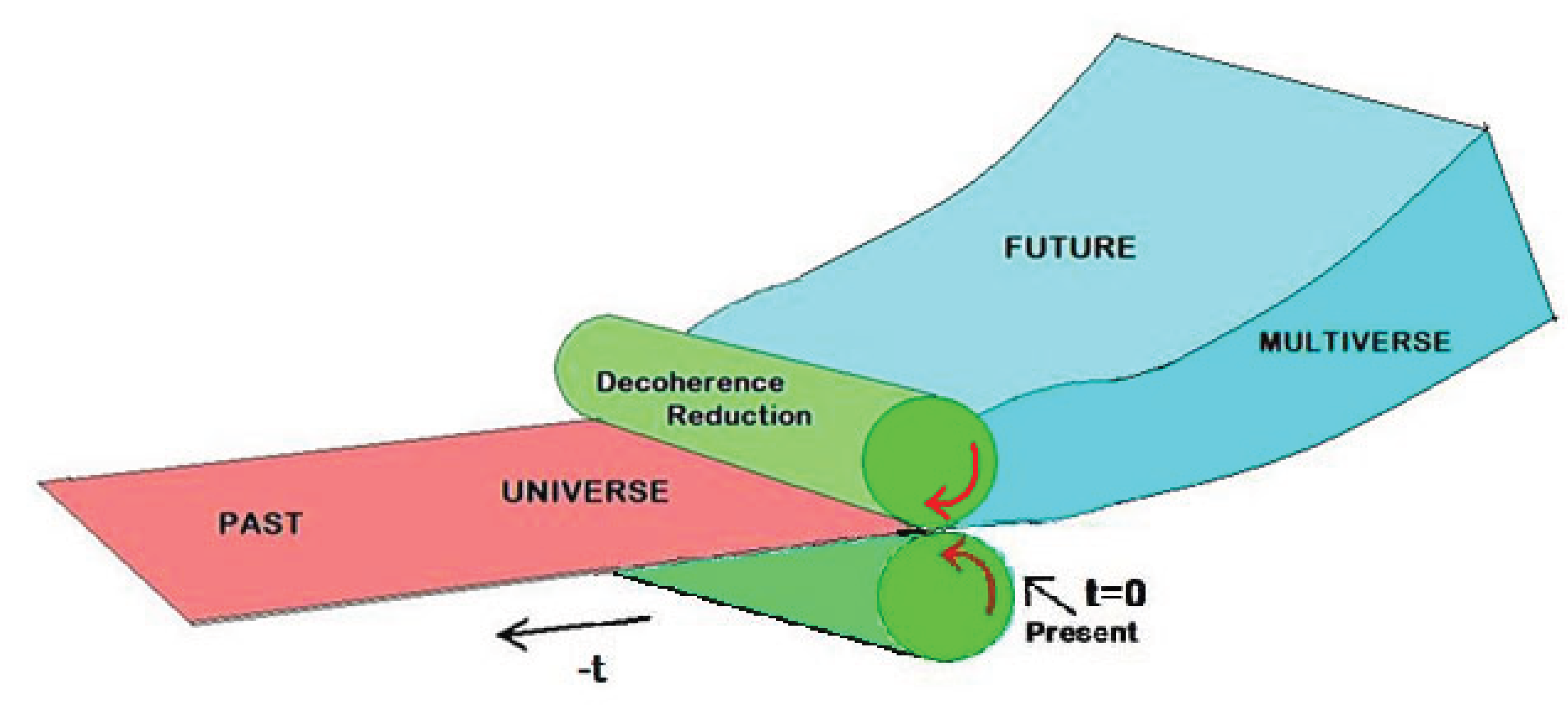
Figure 1. The Universal “Pasta-Maker”.

Figure 1. The Universal “Pasta-Maker”.

Moreover, if many configurations of the universe can be realized in the future, we cannot know which one will actually occur beyond a certain temporal horizon. By contrast, the past consists of fixed events—the realized universe—which we can know but cannot alter.

It is precisely this multitude of possible future states that provides the foundation for the existence of free will. Nonetheless, it still needs to address the underlying law that governs the emergence of order (information handling), in order to fully explain how free will arises (see the second part of the work).

In this context, we can metaphorically illustrate spacetime and its irreversible universal evolution as an enormous pasta maker. In this analogy, the future multiverse is represented by a blob of unshaped flour dough, inflated because it contains all possible states. This dough, extending up to the 4D surface of the present, is then pressed into a thin pasta sheet, representing the quantum superposition projective decay to the classical state realizing the universe. From this standpoint, classical states are ‘re-calculated’ at each instant (in each macroscopic domain) and carried into the future. For instance, we can think of our body as being recalculated at each subsequent state, appearing progressively older as it is carried forward in time. However, in this process, as our present state (both bodily and mental) becomes quantumly decoupled from the previous instant, we simultaneously lose access to, and awareness of, the past universe. As a result, we perceive the external world as a reality in continuous transformation.

The 4D surface boundary between the future multiverse and the past universe marks the instant of present time. At this point, the irreversible process of decoherence occurs, entailing the computation or reduction to the present classical state and generating the direction of time flow. This specific moment defines the present in reality, a notion absent from the relativistic spacetime framework, where time is merely a coordinate that does not flow. The equations of general relativity are timeless in a sense, they describe the whole spacetime at once. In quantum theory of gravity (see for example, the Wheeler-DeWitt equation [38] there is no time at all, everything seems "frozen" and there's no clear way to define "evolution" or "change" as we experience it.

The SQHM marks the point at which irreversibility occurs, setting it apart from other positions along the time axis and giving rise to the dynamics of what we experience as real, unidirectional flowing time.

8. Conclusions

This work presents an ambitious and interdisciplinary proposal, aiming to unify aspects of gravity, quantum physics and classical mechanics within a single theoretical framework.

By bridging diverse domains of physics, this approach integrates quantum and classical physics into a coherent model, particularly through the use of stochastic quantum hydrodynamics. A central idea is the incorporation of stochastic perturbations arising from gravitational background noise, further reinforcing the perspective that the interplay between these two regimes underlies the intricate and emergent nature of our macroscopic reality.

The stochastic quantum hydrodynamic model accurately predicts both the Lindemann constant and the fluid-to-superfluid transition in helium. Furthermore, it addresses the problem of photon quantum entanglement in the context of a finite speed of information transmission, an effect that could be tested in a long-distance, planetary-scale experiment.

The use of Madelung’s quantum hydrodynamic analogy, combined with gravitational stochastic noise, offers a novel framework for understanding how quantum phenomena transition into the classical regime. This approach also tackles fundamental unresolved issues, including the EPR paradox, quantum–classical coexistence, and the origin of time's flow in reality — key challenges in modern theoretical physics.

The work aligns with a school of thought that acknowledges the self-decoherence into a macroscopic reality without requiring a measurement process to determine it. By incorporating quantum uncertainty along with the constraints of finite light speed and information transmission, the theoretical framework proposes that physical spacetime has a discrete nature, allowing for an analogy with the evolution of the universe as a discrete computational simulation. The optimization of this computational process, which leads to the emergence of macroscopic reality, is achieved through the decoherence process, which appears to function as the 'calculation' of the classical state, much like qubits operate in quantum computers.

From this standpoint, classical states are 'recalculated' at discrete instants and propagated into the future. As a result, macroscopic reality manifests a dynamical behavior of continuous macroscopic transformation, where the irreversible nature of quantum decoherence gives rise to the unidirectional flow of time. According to this framework, reality is constrained neither by deterministic laws nor by an unpredictable, probabilistic, measurement-dependent actualization.

References

- Einstein, A., Podolsky, B. and Rosen, N. (1935) Can Quantum-Mechanical Description of Physical Reality Be Considered Complete? Physical Review, 47, 777-780. [CrossRef]
- Bell, J.S. , On the Einstein- Podolsky-Rosen paradox, Physics, 1:195-200 (1964).
- Zurek, W. ,: Decoherence and the Transition from Quantum to Classical—Revisited (https://arxiv.org/pdf/quantph/0306072.pdf), Los Alamos Science Number 27 (2002).
- Mariano, A., Facchi, P. and Pascazio, S. (2001) Decoherence and Fluctuations in Quantum Interference Experiments. Fortschritte der Physik, 49, 1033-1039.
- Cerruti, N.R. , Lakshminarayan, A., Lefebvre, T.H., Tomsovic, S.: Exploring phase space localization of chaotic eigenstates via parametric variation. Phys. Rev. E 63, 016208 (2000). [CrossRef]
- Wang, C. , Bonifacio, P., Bingham, R., Mendonca, J., T., Detection of quantum decoherence due to spacetime fluctuations, 37th COSPAR Scientific Assembly. Held 13-, in Montréal, Canada., p.3390. 20 July.
- Chiarelli, P. Quantum-to-Classical Coexistence: Wavefunction Decay Kinetics, Photon Entanglement, and Q-Bits. Symmetry 2023, 15, 2210. [Google Scholar] [CrossRef]
- Madelung, E. : Z. Phys. 40, 322-6 (1926).
- Bialyniki-Birula, I. , Cieplak, M., Kaminski, J., “Theory of Quanta”, Oxford University press, Ny, (1992) 87-111.
- Weiner, J.H. , Statistical Mechanics of Elasticity (John Wiley & Sons, New York, 1983), p. 315-7.
- Bassi, A.; Großardt, A.; Ulbricht, H. Gravitational decoherence. Class. Quantum Gravity 2016, 34, 193002. [Google Scholar] [CrossRef]
- Chiarelli, P. Can fluctuating quantum states acquire the classical behavior on large scale? Adv. Phys. 2013, 2, 139–163. [Google Scholar]
- Chiarelli, S.; Chiarelli, P. Stochastic Quantum Hydrodynamic Model from the Dark Matter of Vacuum Fluctuations: The Langevin-Schrödinger Equation and the Large-Scale Classical Limit. Open Access Libr. J. 2020, 7, e6659. [Google Scholar] [CrossRef]
- Rumer, Y.B.; Ryvkin, M.S. Thermodynamics, Statistical Physics, and Kinetics; Mir Publishers: Moscow, Russia, 1980; pp. 444–459. [Google Scholar]
- Bressanini, D. An Accurate and Compact Wave Function for the 4 He Dimer. EPL 2011, 96, 23001. [Google Scholar] [CrossRef]
- Gross, E.P. Structure of a quantized vortex in boson systems. Il Nuovo C. 1961, 20, 454–456. [Google Scholar] [CrossRef]
- Pitaevskii, P.P. Vortex lines in an Imperfect Bose Gas. Sov. Phys. JETP 1961, 13, 451–454. [Google Scholar]
- Rumer, Y.B.; Ryvkin, M.S. Thermodynamics, Statistical Physics, and Kinetics; Mir Publishers: Moscow, Russia, 1980; p. 260. [Google Scholar]
- Chiarelli, P. The quantum potential: The missing interaction in the density maximum of He4 at the lambda point? J. Phys. Chem. 2014, 2, 122–131. [Google Scholar] [CrossRef]
- Andronikashvili, E.L. Zh. Éksp. Teor. Fiz 1946, 16, 780; 1948, 18, 424. [Google Scholar]
- Gardiner, C.W. Handbook of Stochastic Method, 2nd ed.; Springer: Berlin/Heidelberg, Germany, 1985; pp. 195–210. ISBN 3-540-61634. [Google Scholar]
- Ruggiero, P.; Zannetti, M. Quantum-classical crossover in critical dynamics. Phys. Rev. B 1983, 27, 3001. [Google Scholar] [CrossRef]
- Ruggiero, P.; Zannetti, M. Critical Phenomena at T = 0 and Stochastic Quantization. Phys. Rev. Lett. 1981, 47, 1231. [Google Scholar] [CrossRef]
- Ruggiero, P.; Zannetti, M. Microscopic derivation of the stochastic process for the quantum Brownian oscillator. Phys. Rev. A 1983, 28, 987. [Google Scholar] [CrossRef]
- Ruggiero, P.; Zannetti, M. Stochastic description of the quantum thermal mixture. Phys. Rev. Lett. 1982, 48, 963. [Google Scholar] [CrossRef]
- Kleinert, H.; Pelster, A.; Putz, M.V. Variational perturbation theory for Marcov processes. Phys. Rev. E 2002, 65, 066128. [Google Scholar] [CrossRef] [PubMed]
- Chiarelli, P. The Stochastic Nature of Hidden Variables in Quantum Mechanics. Hadron. J. 2023, 46, 315–338. [Google Scholar]
- Santilli, R.M. A Quantitative Representation of Particle Entanglements via Bohm’s Hidden Variable According to Hadronic Mechanics. Prog. Phys. 2002, 1, 150–159. [Google Scholar]
- Ghirardi, G.C.; Rimini, A.; Weber, T. Unified dynamics for microscopic and macroscopic systems. Phys. Rev. D 1986, 34, 470–491. [Google Scholar] [CrossRef]
- Pearle, P. Combining stochastic dynamical state-vector reduction with spontaneous localization. Phys. Rev. A 1989, 39, 2277–2289. [Google Scholar] [CrossRef]
- Diósi, L. Models for universal reduction of macroscopic quantum fluctuations. Phys. Rev. A 1989, 40, 1165–1174. [Google Scholar] [CrossRef]
- Penrose, R. On Gravity’s role in Quantum State Reduction. Gen. Relativ. Gravit. 1996, 28, 581–600; [Google Scholar] [CrossRef]
- Chiarelli, P. , Quantum Spacetime Geometrization: QED at High Curvature and Direct Formation of Supermassive Black Holes from the Big Bang, Quantum Rep. 2024, 6, 14–28. [CrossRef]
- Chiarelli, P. The Gravity of the Classical Klein-Gordon Field. Symmetry 2019, 11, 322. [Google Scholar] [CrossRef]
- Chiarelli, P. Quantum Geometrization of Spacetime in General Relativity; BP International: Hong Kong, China, 2023; ISBN 978-81-967198-7-6. [Google Scholar] [CrossRef]
- Valev, D. Estimation of Total Mass and Energy of the observable Universe. Phys. Int. 2014, 5, 15–20. [Google Scholar] [CrossRef]
- Makeenko, Y. Methods of Contemporary Gauge Theory; Cambridge University Press: Cambridge, UK, 2002; ISBN 0-521-80911-8. [Google Scholar]
- DeWitt, B.S. Quantum Theory of Gravity. I. The Canonical Theory. Phys. Rev. 1967, 160, 1113–1148. [Google Scholar]
Disclaimer/Publisher’s Note: The statements, opinions and data contained in all publications are solely those of the individual author(s) and contributor(s) and not of MDPI and/or the editor(s). MDPI and/or the editor(s) disclaim responsibility for any injury to people or property resulting from any ideas, methods, instructions or products referred to in the content. |
© 2025 by the authors. Licensee MDPI, Basel, Switzerland. This article is an open access article distributed under the terms and conditions of the Creative Commons Attribution (CC BY) license (http://creativecommons.org/licenses/by/4.0/).
Copyright: This open access article is published under a Creative Commons CC BY 4.0 license, which permit the free download, distribution, and reuse, provided that the author and preprint are cited in any reuse.