
Submitted:
03 December 2025
Posted:
04 December 2025
Read the latest preprint version here
Abstract
A harmonic analysis of Antarctic ice core proxy temperature, CO₂ and CH₄ data is presented spanning 350,000 years. Using a greedy algorithm to select periodic components, the analysis initially obtained 59 periods for temperature but subsequently refined this to 55 periods after removing four components (22,150, 9,000, 8,000, and 4,540 years) that exhibited high correlations in the normalized covariance matrix. This refinement ensures stable, well- conditioned parameter estimates while maintaining excellent fits: R² = 0.952 for temperature and R² = 0.964 for CO₂ (truncated at 1850 CE), R² = 0.873 for CH₄ . The algorithm independently recovers the canonical Milankovitch orbital periods (approximately 100,000, 41,000, and 23,000 years) without prior specification, validating both the methodology and the orbital pacing of ice ages (Milankovitch, 1941). Phase analysis reveals that CO₂ consistently lags temperature by 600–4,000 years at orbital timescales, supporting the hypothesis that temperature drives CO₂ through ocean degassing rather than the reverse. Examination of the Last Interglacial (Eemian) reveals a striking asymmetry: CO₂ remained elevated at 275–280 ppm for approximately 13,000 years while temperature declined by 7°C. An R² analysis clearly reveals the Mid-Pleistocene Transition and justifies limiting the input to the fit. The modern CO₂ spike, which departs dramatically from the 350,000-year orbital envelope, is clearly anomalous relative to the harmonic structure of the paleoclimate record.
Keywords:
ice-core
; Antarctic
; CO2
; CH4
1. Introduction
The relationship between atmospheric CO2 and temperature over glacial-interglacial cycles has been extensively studied using ice core records. A central question concerns causality: does CO2 drive temperature through radiative forcing, or does temperature drive CO2 through effects on ocean solubility, biological productivity, and terrestrial carbon storage?
Previous studies have established that CO2 variations lag temperature changes during glacial terminations by several hundred to a few thousand years (Humlum et al., 2013; Grabyan, 2025). However, the precise phase relationship varies across different studies depending on methodology. Here we apply harmonic analysis with a novel period-selection algorithm to Antarctic ice core data spanning the last 350,000 years.
2. Data and Methods
2.1. Data Source
We analyze Antarctic ice core data converted to proxy temperature from the EPICA Dome C record (Jouzel et al., 2007), comprising 4,752 data points covering the interval from 350,245 years before present to 1911 CE. The corresponding CO2 record (Bereiter et al., 2015) extends to 2001 CE. To avoid potential complications from apparent changes in interglacial maxima around 450,000 BCE (Higginbotham, 2025), the data interval used in the fit is from 350,000 BCE to present, or to 1850 CE for CO2 to exclude anthropogenic influence. The Mid-Pleistocene Transition (MPT) associated with changes around 450,000 BCE is discussed below with respect to the temperature fit.
In the tables and figures that follow, negative dates will correspond to BCE while positive dates will correspond to CE.
Temperature: EPICA Dome C deuterium-derived temperature proxy (Jouzel et al., 2007), EDC3 chronology, 4,752 data points from 350,245 years BP to 1911 CE.
CO2: Antarctic composite record (Bereiter et al., 2015), AICC2012 chronology. Data truncated at 1850 CE to exclude anthropogenic influence. The fit involved 1130 data points from 350,000 BCE to 1850 CE.
CH4: EPICA Dome C methane record (Loulergue et al., 2008), EDC3 gas age chronology, matching the temperature chronology. The fit involved 1418 data points from 350,000 BCE to 1824 CE.
2.2. Harmonic Fitting Methodology
We fit each dataset to a harmonic model of the form:
X(t) = C + Σᵢ Aᵢ sin(2π(t − t₀)/Pᵢ + φᵢ)
where C is a constant offset, t₀ is the time origin (−175,000 years for all fits to allow direct comparison of phase), and each periodic component has amplitude Aᵢ, period Pᵢ, and phase φᵢ. For computational stability, the model is implemented using sine and cosine basis functions:
X(t) = C + Σᵢ [aᵢ sin(2π(t − t₀)/Pᵢ) + bᵢ cos(2π(t − t₀)/Pᵢ)]
where amplitude A = √(a2 + b2) and phase φ = atan2(a, b). This parameterization avoids nonlinear optimization over phase.
2.3. Greedy Period Selection Algorithm
Rather than using predetermined periods or standard Fourier analysis, we employ a "greedy" algorithm: beginning with a constant term, iteratively add the period that most reduces residual variance, searching continuously over period space. The algorithm includes safeguards against ill-conditioning: minimum period separation, rejection of candidates causing excessive amplitude changes in existing periods, and amplitude ceilings.
2.4. Covariance Matrix Analysis and Period Refinement
To verify that selected periods form a well-conditioned basis, we computed the normalized covariance matrix for fitted parameters. Off-diagonal elements near ±1 indicate near-collinearity, which inflates parameter uncertainties.
Using temperature as an example
Initial analysis of the 59-period fit to temperature revealed problematic correlations:
- Periods 7,600 yr and 4,540 yr: r = −0.95
- Periods 8,900 yr and 9,000 yr: r = −0.70
- Periods 7,900 yr and 8,000 yr: r = −0.61
- Periods 23,000 yr and 22,150 yr: r = −0.51
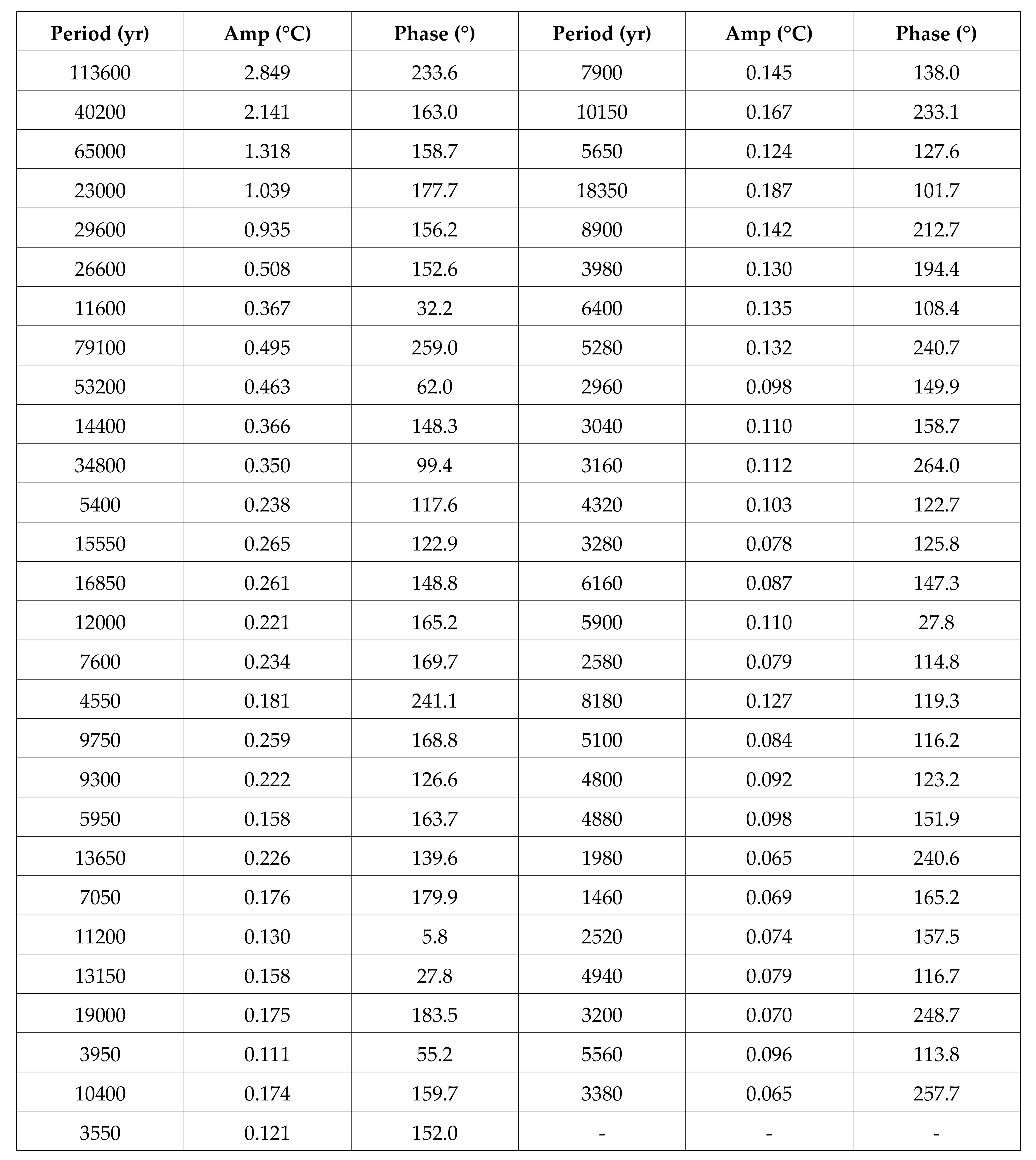
We systematically removed the higher-index period from each problematic pair: 4,540, 9,000, 8,000, and 22,150 years. The final 55-period basis shows maximum off-diagonal correlations of |r| ≈ 0.15 for temperature and |r| ≈ 0.52 for CO2—acceptable levels for stable parameter estimation.

Table 1.
Fit quality before and after covariance refinement.
| Configuration | R2 (Temperature) | Max |r| |
|---|---|---|
| Original (59 periods) | 0.9539 | 0.95 |
| Refined (55 periods) | 0.9517 | 0.15 |
The minimal R2 change (0.0022) confirms these components were largely redundant.
Where CO2 and CH4 were independently fit, the same procedure was followed to obtain a good R2 with acceptable |r|.
2.5. Uncertainty Estimation from Covariance Matrix
The unnormalized covariance matrix provides variances for each fitted parameter. Standard errors (SE) on sine and cosine coefficients propagate to amplitude and phase uncertainties via:
SE(A) = √[(a/A)2 var(a) + (b/A)2 var(b)]
SE(φ) = (180/π) × √[(b/A2)2 var(a) + (a/A2)2 var(b)]
Phase lag uncertainties combine temperature and CO2 phase uncertainties in quadrature: SE(lag) = (P/360°) × √[SE(φ_T)2 + SE(φ_CO2)2].
2.6. CO2 Fitting with Periods Found for Temperature
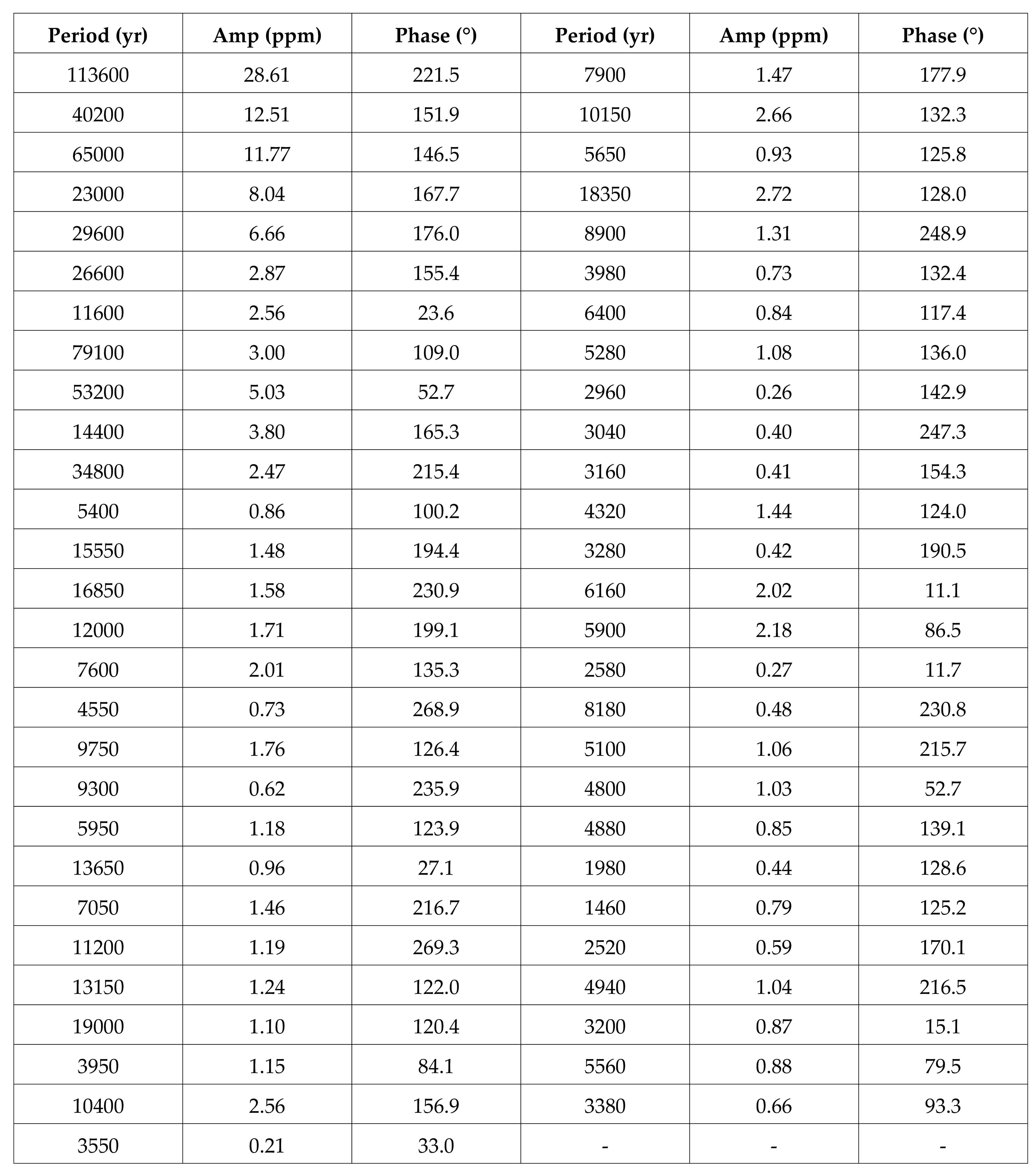
We fit CO2 data to the same 55 periods with constant, allowing only amplitudes and phases to vary. Data after 1850 CE was excluded. The truncated fit achieves R2 = 0.964, with maximum off-diagonal correlation |r| = 0.52. See Appendix A for further comments.The fit involved 1130 data points.
2.7. CO2 Fitting with Periods Found Independently
The fit to CO2 with periods found independently, with data after 1850 CE excluded, used a constant and 31 periods achieving an R2 = 0.958, with maximum off-diagonal correlation |r| = 0.47. The fit involved 1130 data points.
2.8. CH4 Fitting with Periods Found Independently
The fit to CH4 with periods found independently used a constant and 55 periods achieving an R2 = 0.873, with maximum off-diagonal correlation |r| = 0.40 .The fit involved 1418 data points.
3. Results
3.1. Temperature Fit Quality
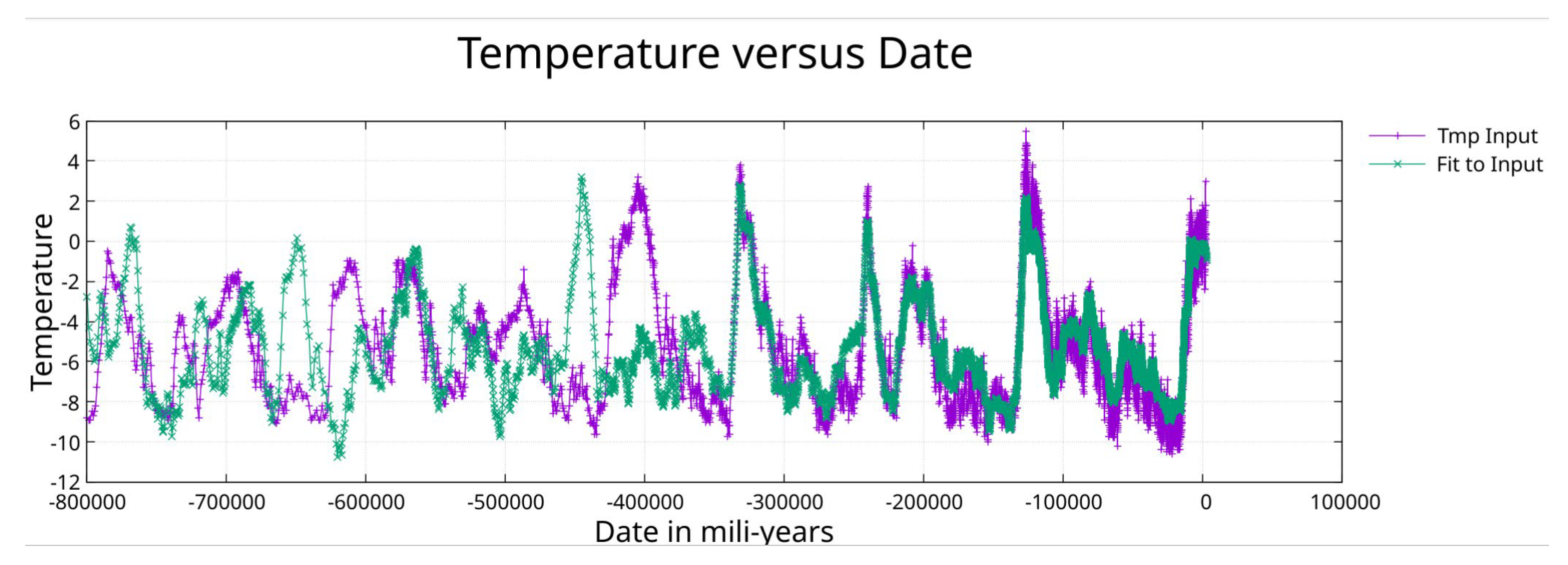
The 55-period fit achieves R2 = 0.952, explaining over 95% of variance in the 350,000-year record. The fit tracks glacial-interglacial cycles, the Eemian peak, the last deglaciation, the Younger Dryas, and millennial-scale Holocene variations including the Little Ice Age. See Appendix B for more details and fit amplitudes.
Figure 1.
Fit to temperature proxy from date -350,000 to date 1850.
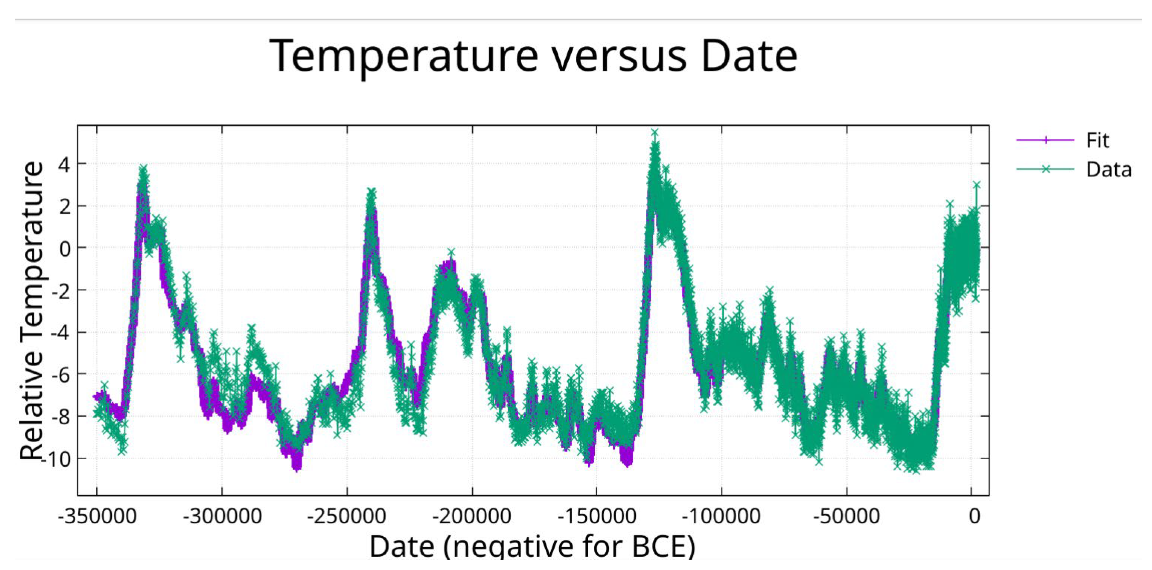
Figure 2.
Fit to Temperature proxy from the prior interglacial warm period to date 1850.
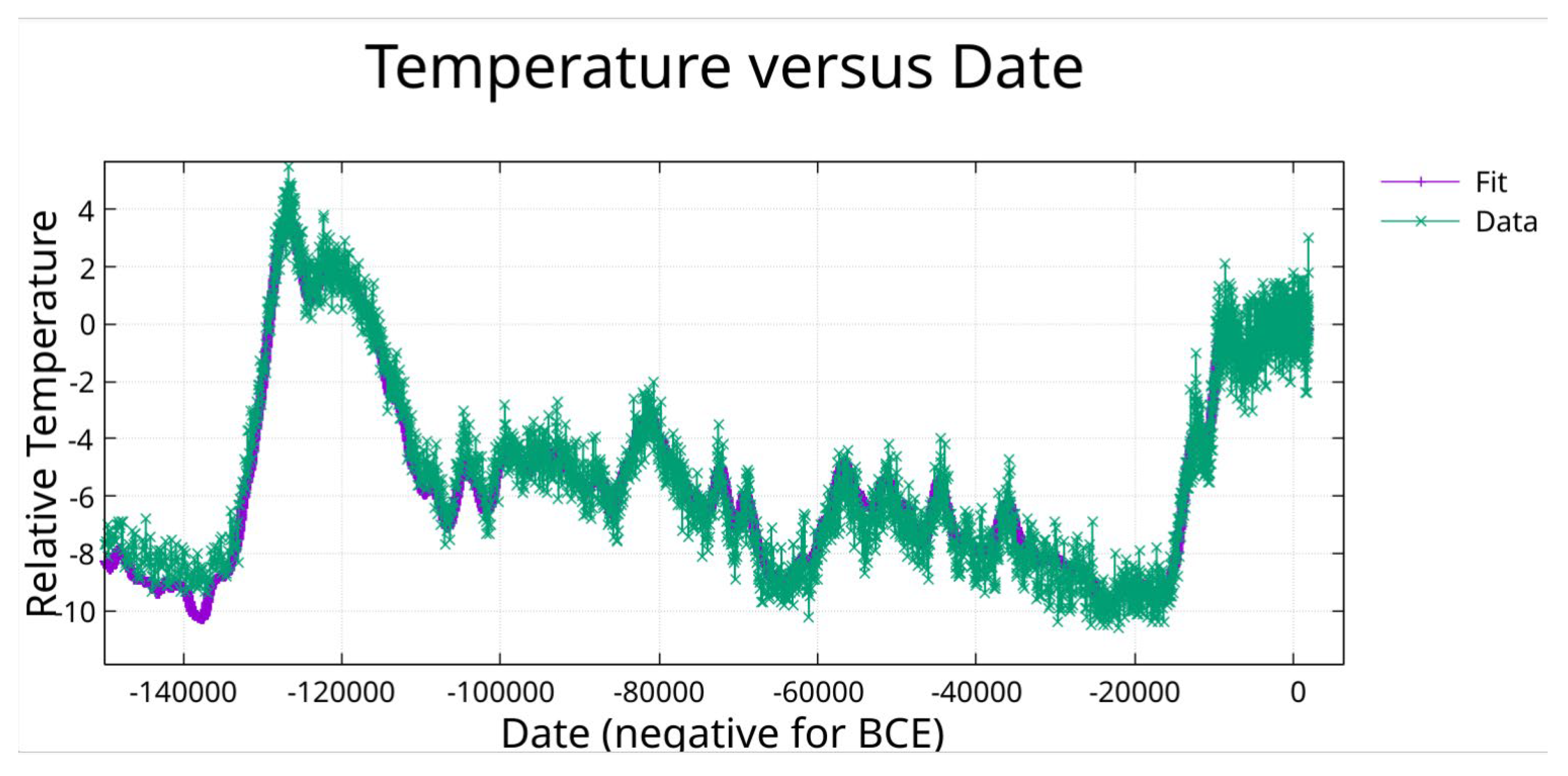
Figure 3.
Fit to Temperature proxy from date -25,000 to date 1850.
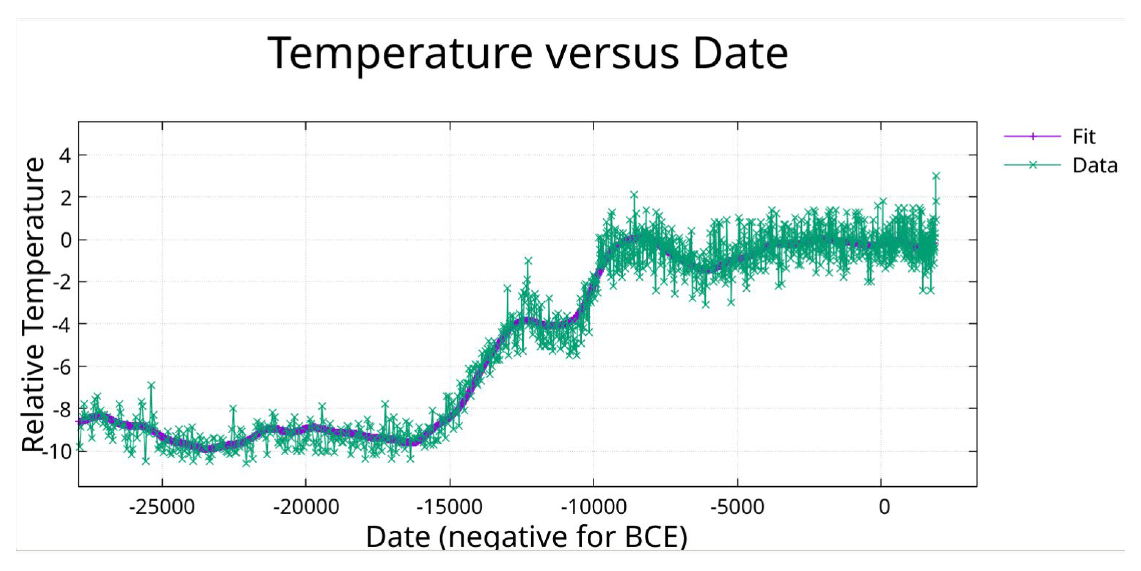
Figure 4.
Fit to Temperature proxy from date -12,000 to date 1850.
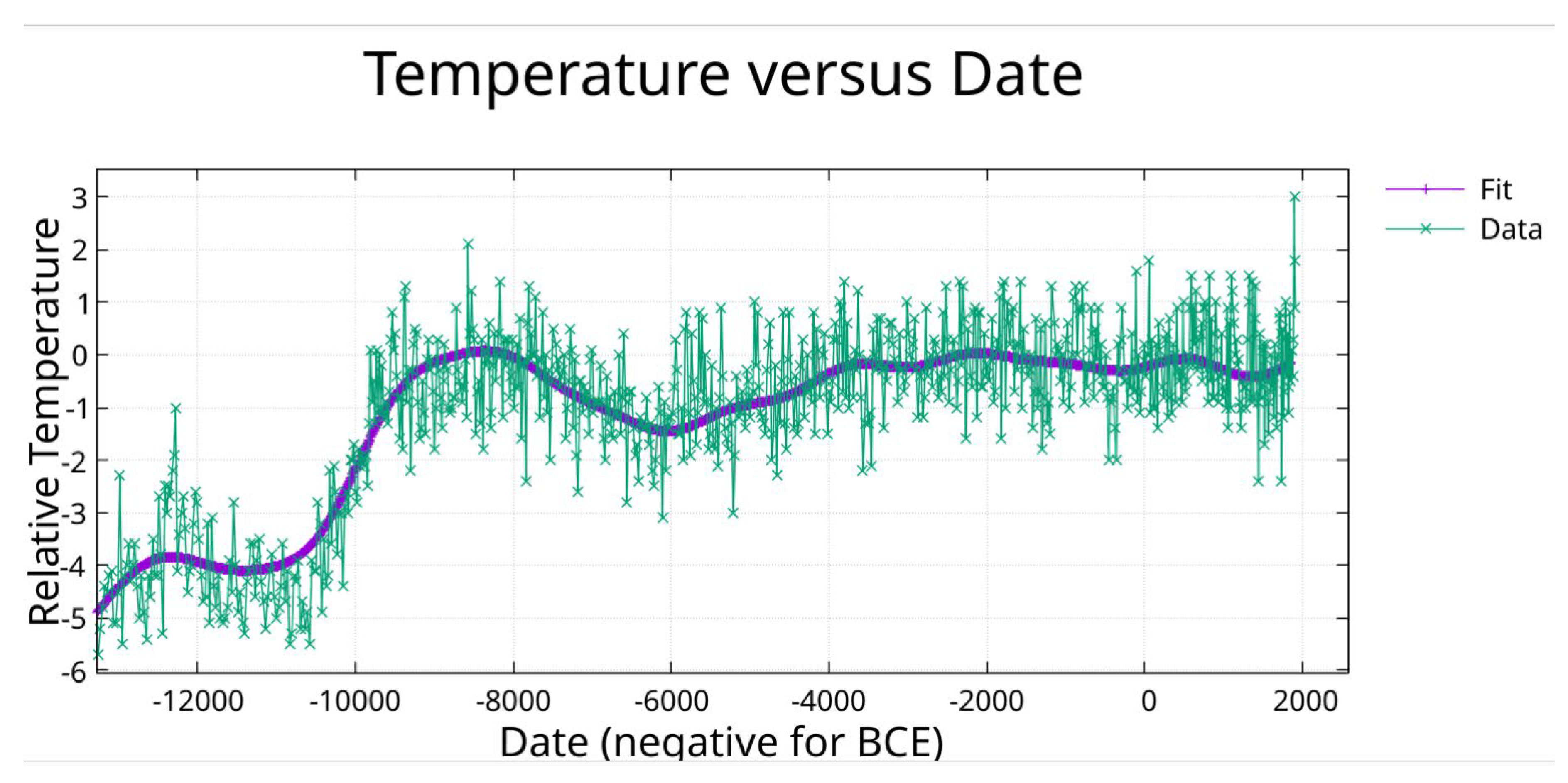
Figure 5.
Fit of CO2 (periods from temperature fit) in ppm from date -350,000 to 1850.
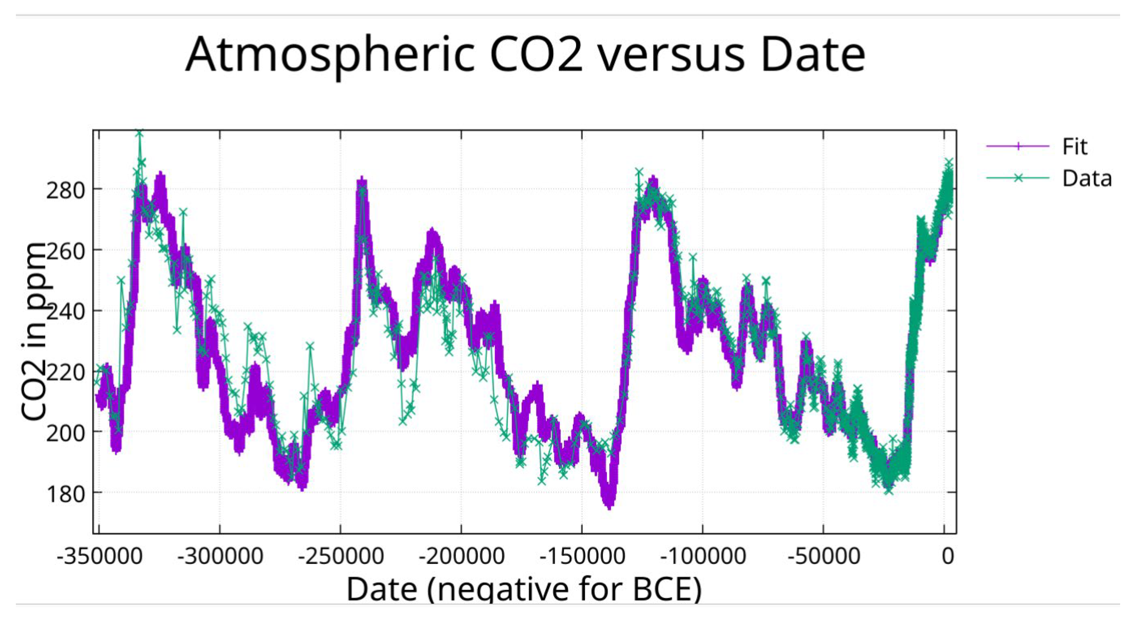
Figure 6.
Fit of CO2 (periods from temperature fit) in ppm from prior interglacial warm period to date 1850.
Figure 6.
Fit of CO2 (periods from temperature fit) in ppm from prior interglacial warm period to date 1850.
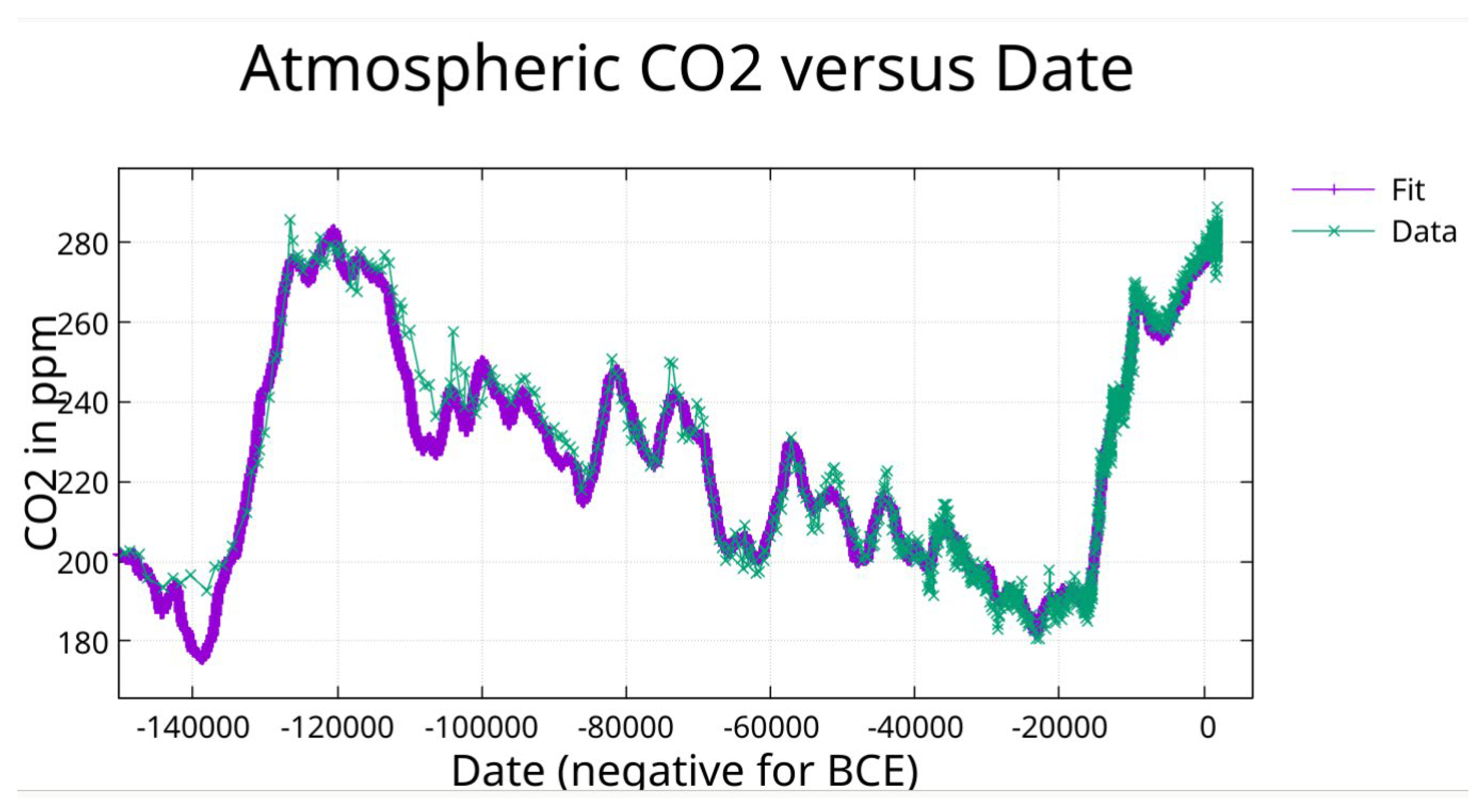
Figure 7.
Fit of CO2 (periods from temperature fit) in ppm from date -25,000 to date 1850.
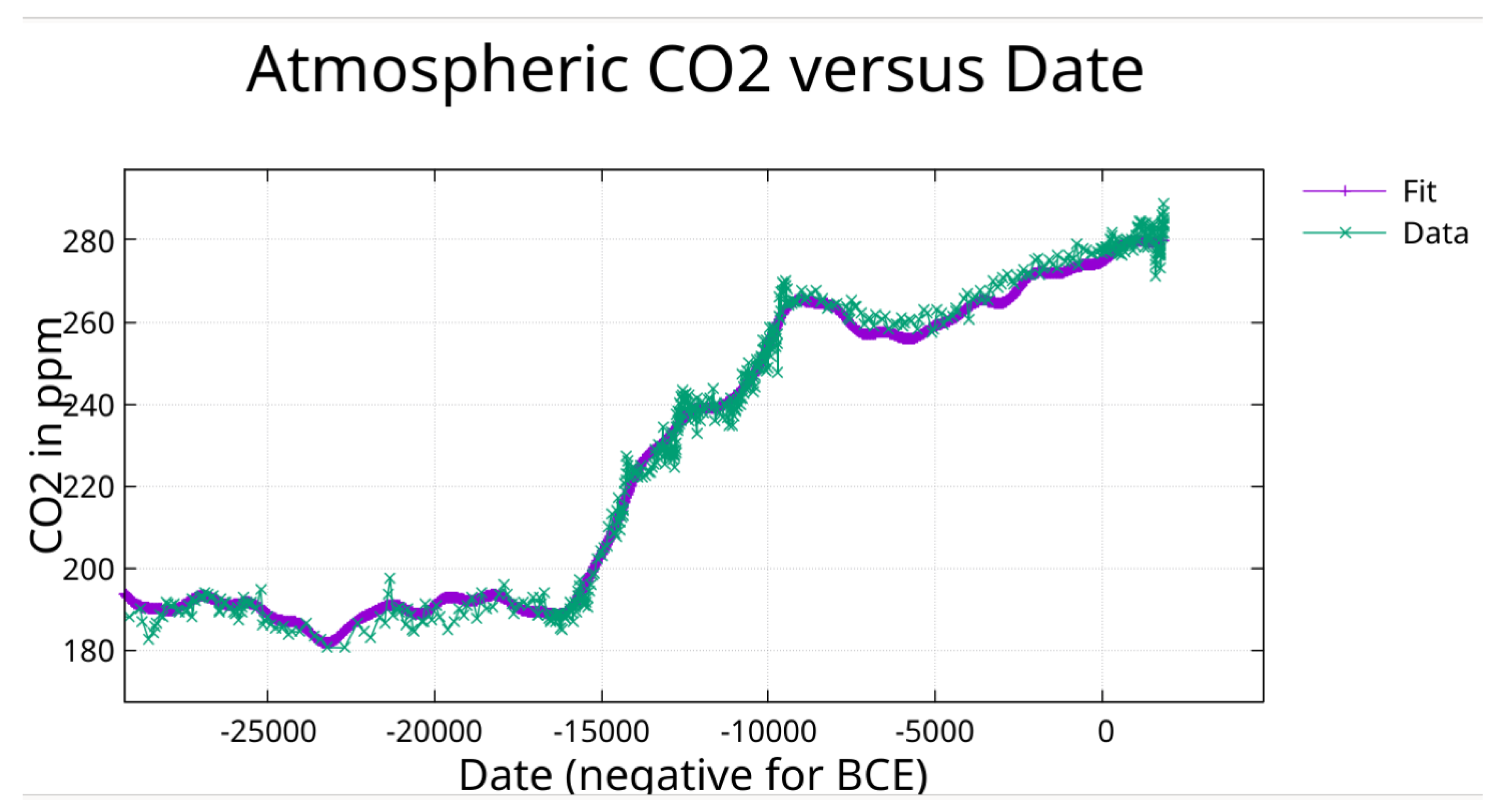
Figure 8.
Fit of CO2 (periods from temperature fit) in ppm from date -12,000 to date 1850. There is an obvious separation of the fit from the data for the last 10,000 years for this case that is not in the fit where periods are found independently. The data itself show larger excursions between dates 1500 and 1850 .
3.2. Recovery of Milankovitch Periods
The algorithm independently recovered periods matching canonical Milankovitch cycles (Milankovitch, 1941):
3.3. CO2 Fit Using Periods from Temperature Fit and Phase Analysis
The CO2 fit, using periods from the temperature fit, achieves R2 = 0.964. For phase comparison, amplitudes were normalized to positive values (adding 180° to phase when amplitude was negative). Phase lag = (Δφ/360°) × P, with negative values indicating CO2 lagging temperature. See Appendix C for fit amplitudes.
The fit of CO2 data to the same periods was done: (1) to determine if the same periods would fit the CO2 data, (2) to allow direct comparison of phase for each period. Additionally, it turned out that subsequently fitting the entire set of data from ~800,000 BCE to 1911 revealed the Mid-Pleistocene Transition which is discussed below.
A fit of CO2 data using the greedy algorithm with pruning will be presented and discussed below.
3.4. Phase Lag Results with Uncertainties Where Both Fits Use the Same Periods
Table 2.
Phase relationships for dominant periods (55-period fit).
| Period (yr) | T Phase (°) | CO2 Phase (°) | Lag (yr) | SE(lag) | Cycle |
|---|---|---|---|---|---|
| 113,600 | 233.6 | 221.5 | −3,818 | ±10,400 | Eccentricity |
| 40,200 | 163.0 | 151.9 | −1,239 | ±5,100 | Obliquity |
| 65,000 | 158.7 | 146.5 | −2,203 | ±13,300 | — |
| 23,000 | 177.7 | 167.7 | −639 | ±5,500 | Precession |
| 29,600 | 156.2 | 176.0 | +1,628 | ±8,600 | — |
| 26,600 | 152.6 | 155.4 | +207 | ±13,800 | — |
The large formal uncertainties reflect the challenge of precisely determining phases for individual sinusoidal components in a multi-period decomposition. However, the consistent pattern of negative lags (CO2 lagging temperature) across the three major Milankovitch periods provides collective evidence stronger than any single period alone. The complete phase lag analysis for all 55 periods is provided in Appendix E.
The fit of CO2 data using the greedy algorithm with pruning (31 periods), and a fit of the CH4 data using the greedy algorithm with pruning are discussed below. The phase issue for these fits is addressed with cross-correlation.
3.5. The Eemian CO2 Plateau
The Last Interglacial reveals profound asymmetry: from −130,000 to −117,000 years, temperature declined ~7°C while CO2 remained at 275–280 ppm. This 13,000-year plateau indicates CO2 absorption during cooling is much slower than release during warming.
3.6. Mid-Pleistocene Transition (MPT)
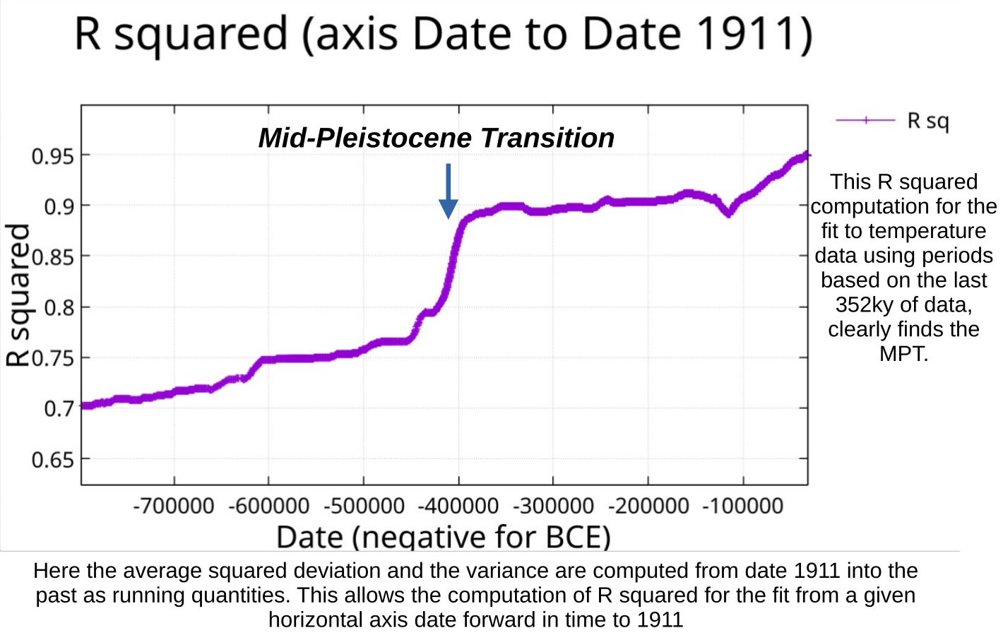
Consistent with the (MPT) (Clark et al., 2006; Berends et al., 2021), Figure 9 indicates that the periods that fit the data well from date -350,000 to 1911 are not appropriate for the temperature variations prior to date -400,000. The R squared value for this plot was 0.7.
The dominant ~100,000-year eccentricity cycle that characterizes the late Pleistocene is largely absent in the earlier record, which was dominated by the ~41,000-year obliquity cycle. The fit using periods determined on data from date -350,000 and later appears to be almost orthogonal to the data prior to date -400,000.
Figure 10 shows how a running computation of R squared produces a sharp drop for this fit at date -400,000 (400,000 BCE).
Figure 10.
Here the average squared deviation and the variance are computed from date 1911 into the past as running quantities. This allows the computation of R squared for the fit from a given horizontal axis date forward in time to 1911.
Figure 10.
Here the average squared deviation and the variance are computed from date 1911 into the past as running quantities. This allows the computation of R squared for the fit from a given horizontal axis date forward in time to 1911.
Figure 11.
CO2 fit with periods found using the greedy algorithm followed by pruning to minimumize off diagonal correlation.
Figure 11.
CO2 fit with periods found using the greedy algorithm followed by pruning to minimumize off diagonal correlation.
Figure 12.
Zoom on previous plot of Fit to CO2.
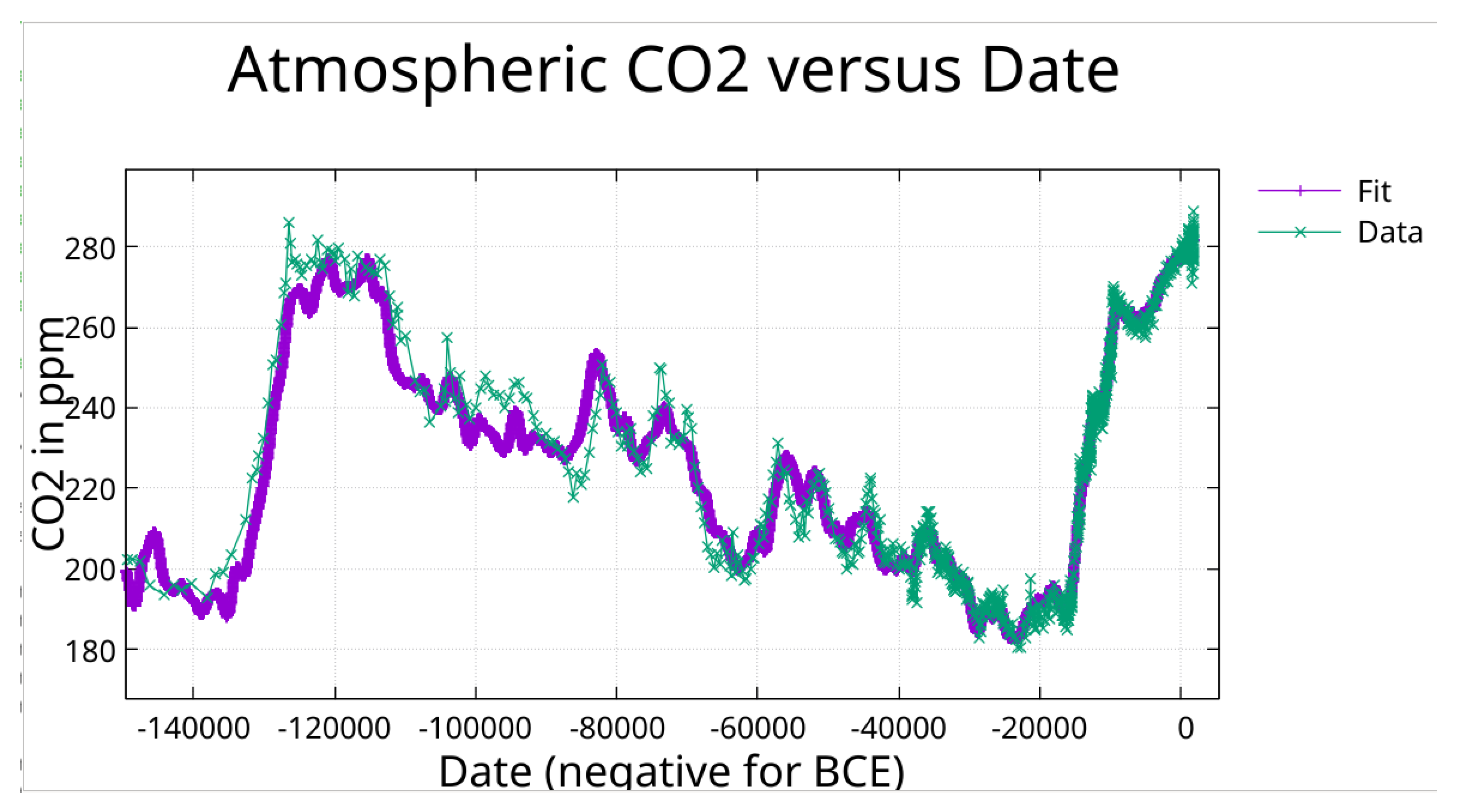
Figure 13.
Zoom on previous plot of CO2.
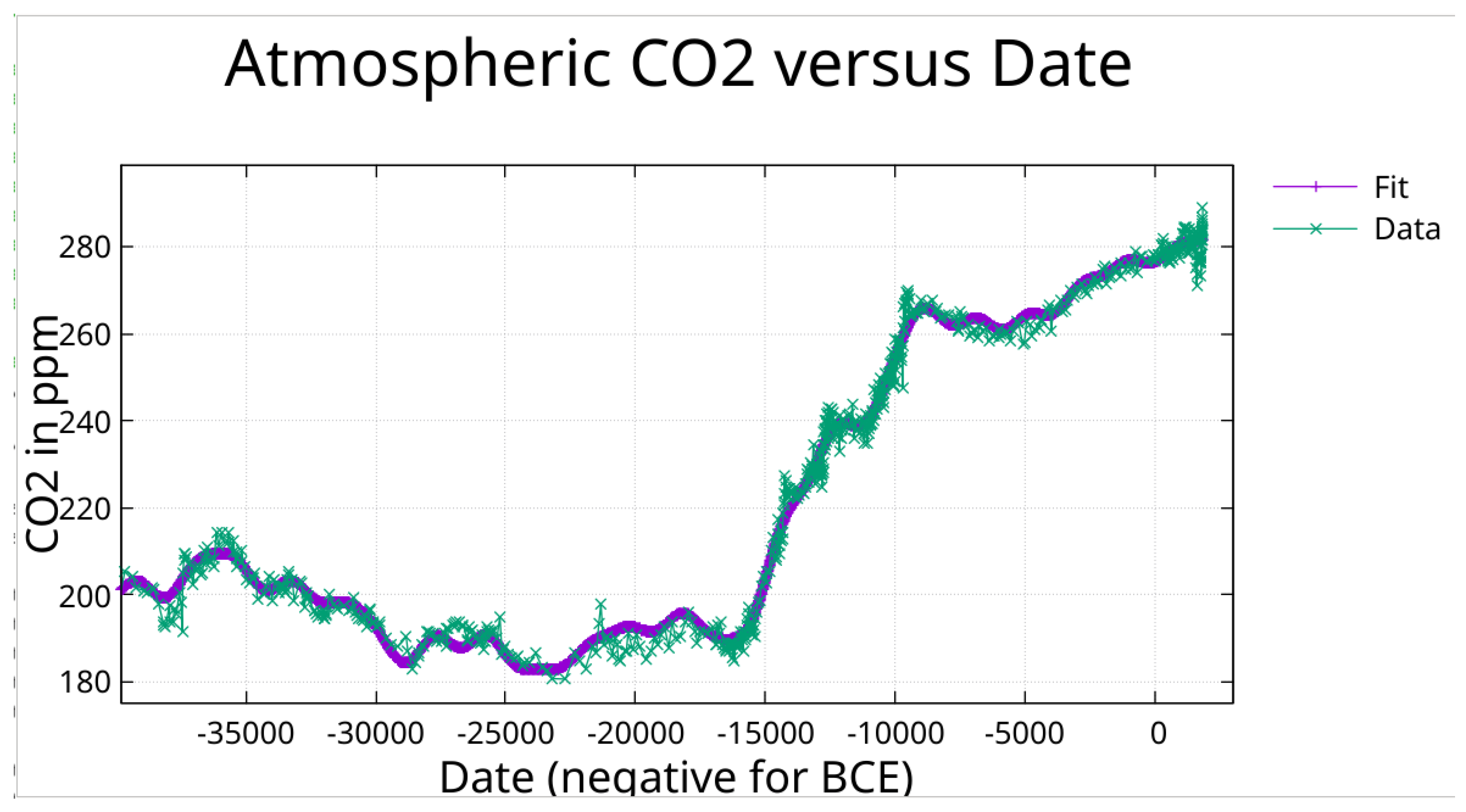
Figure 14.
Zoom on previous plot. Compare to Figure 8.
Figure 14.
Zoom on previous plot. Compare to Figure 8.
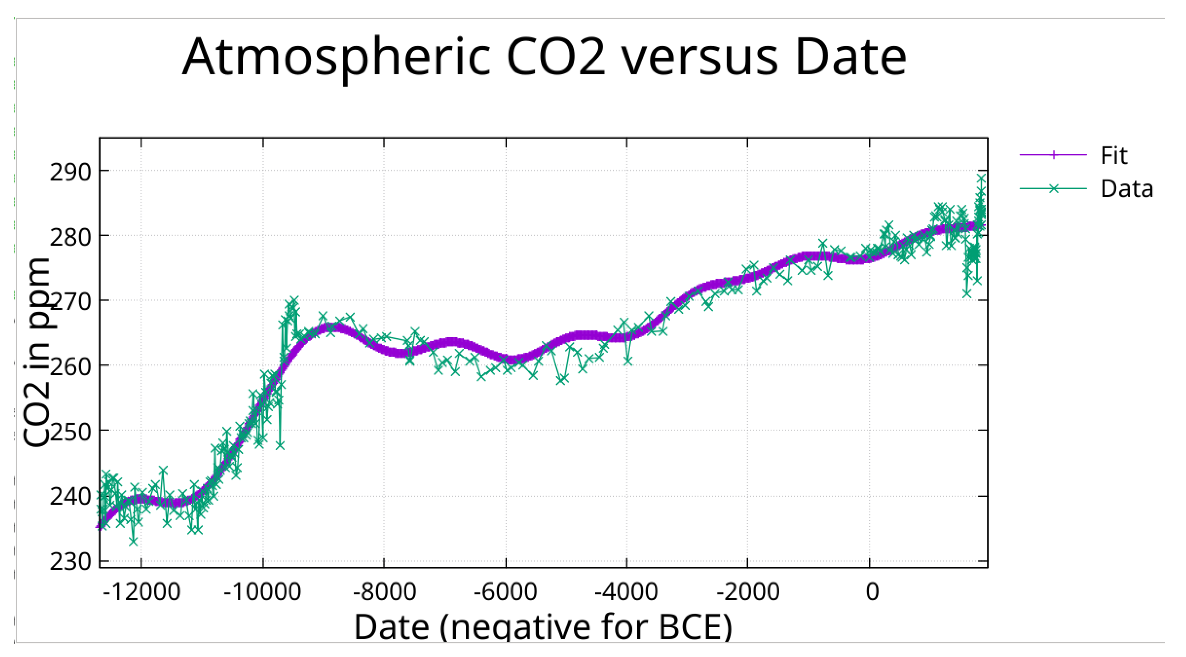
Figure 15.
CH4 fit with periods found by greedy algorithm followed by pruning to minimize off diagonal correlation.
Figure 15.
CH4 fit with periods found by greedy algorithm followed by pruning to minimize off diagonal correlation.
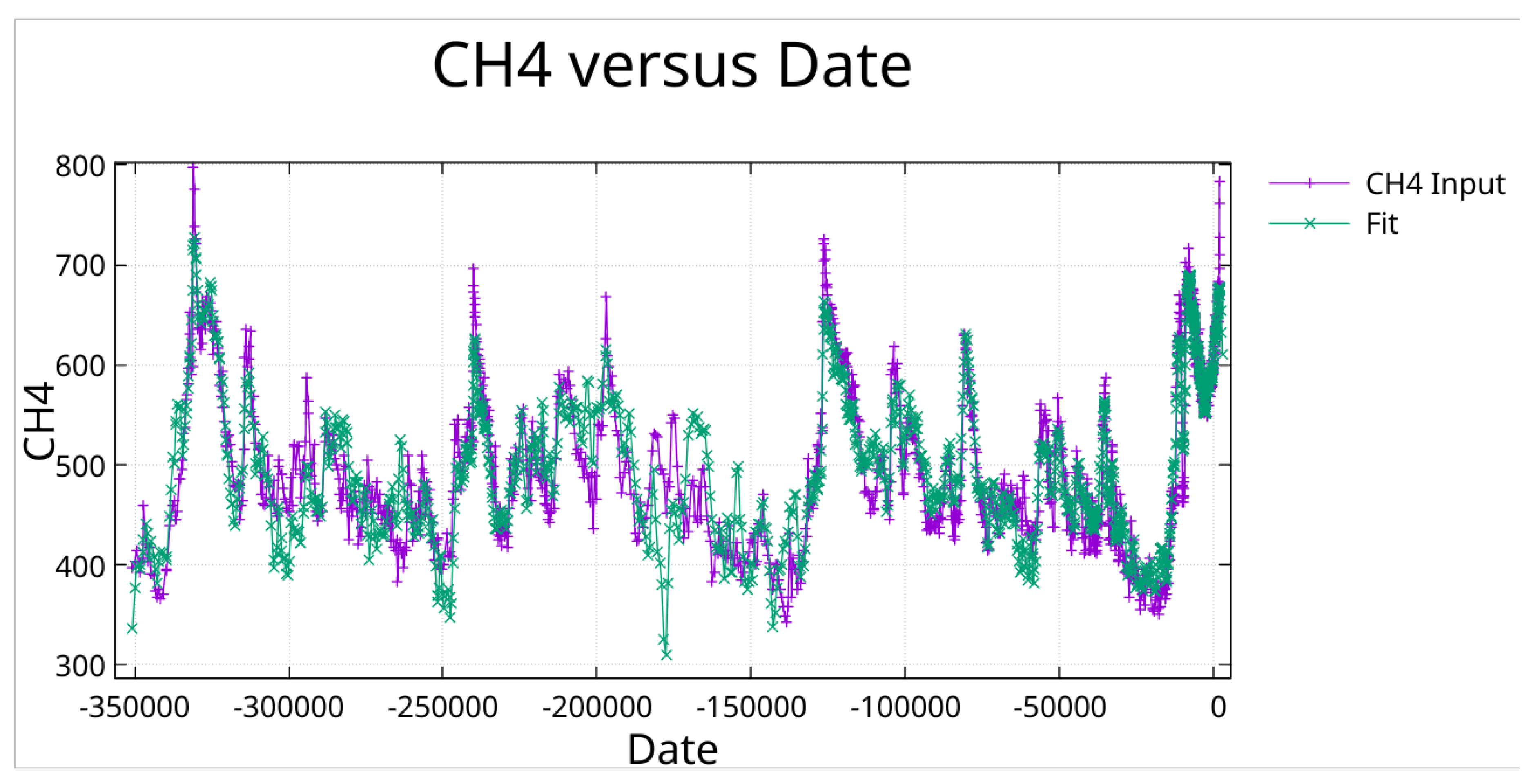
Figure 16.
Zoom on previous Figure.
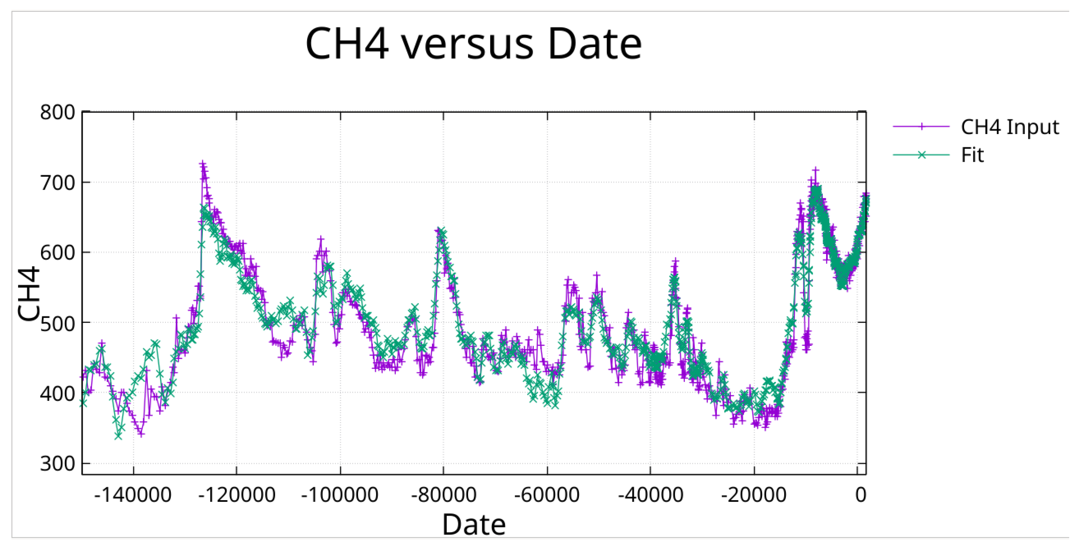
Figure 17.
Zoom on previous Figure. Note the fit to the Younger Dryas notch at around 10,000 BCE.
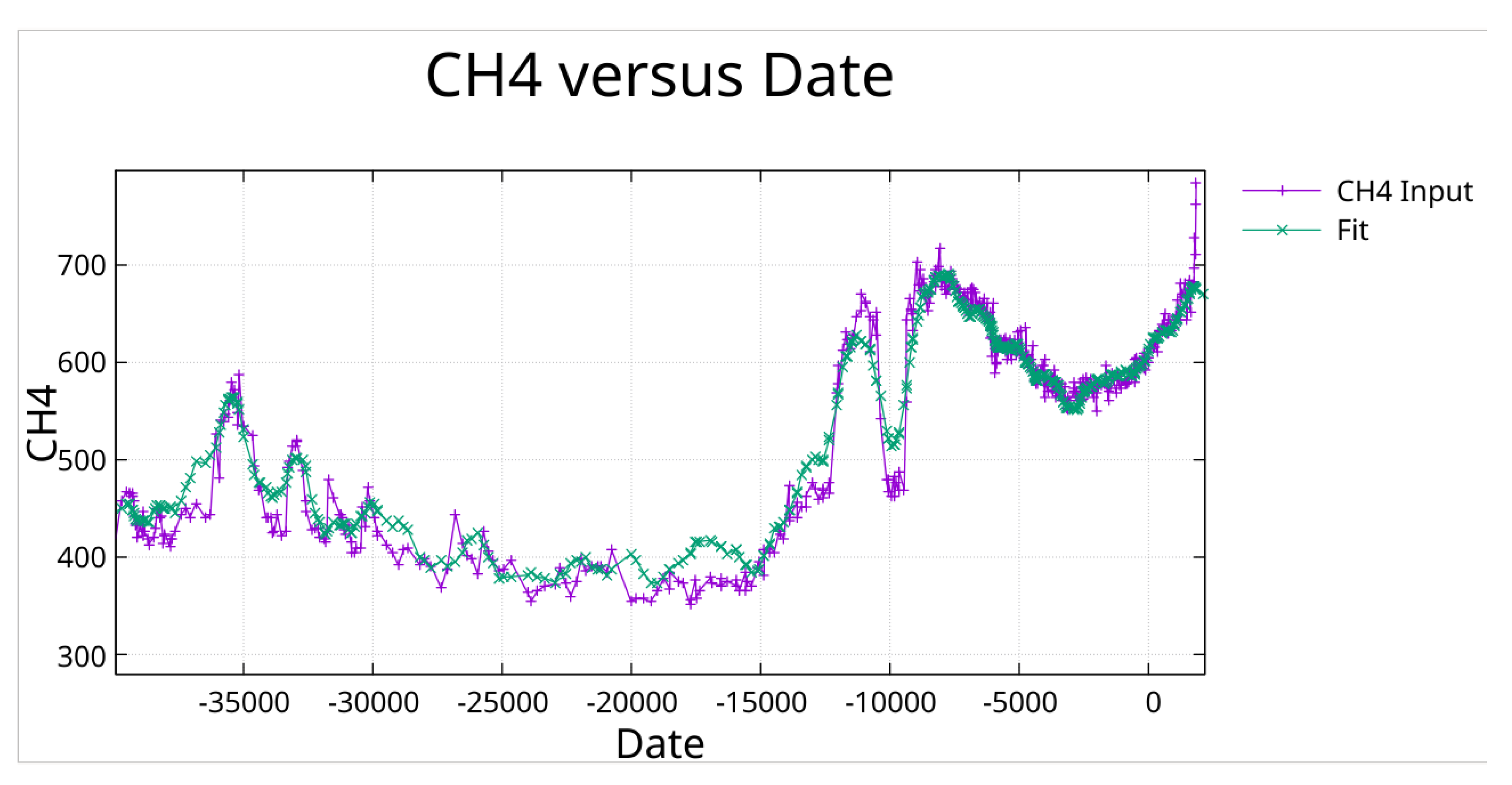
Figure 18.
Zoom on previous Figure showing more clearly the fit to the Younger Dryas.
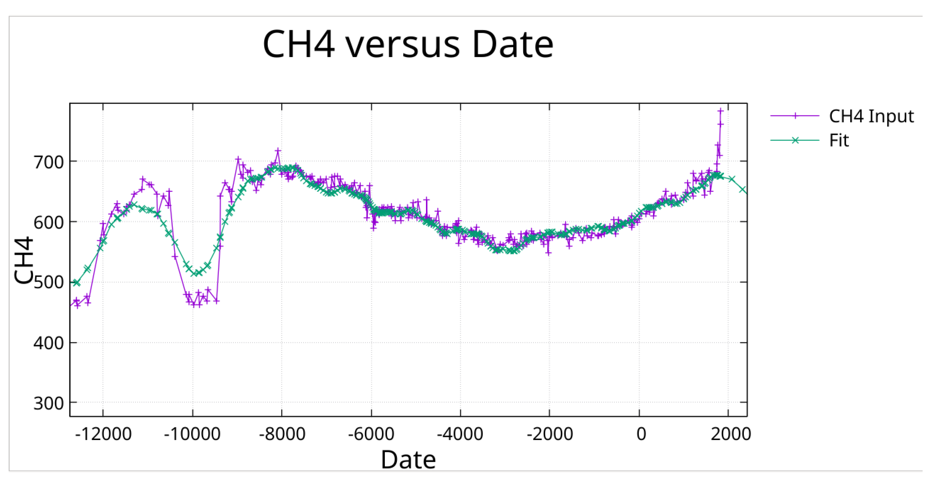
Figure 19.
The times series for temperature and CO2 for intervals, 350,000 BCE -1850 CE, 175,000 BCE – 1850 CE, 120,000 BCE – 1850 CE, and 60,000 BCE – 1850 CE, were cross correlated. The results are plotted here showing a lag in CO2 that decreases as the input is restricted to more recent data until leading temperature for the case of 60,000 BCE – 1850 CE.
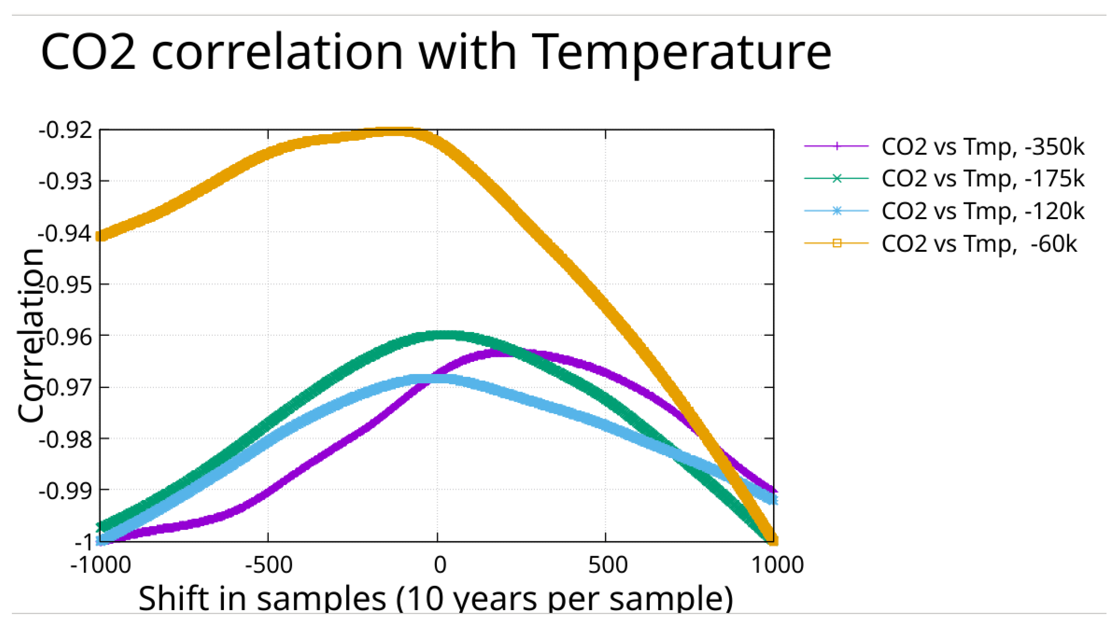
Figure 20.
The times series for temperature and CH4 for intervals, 350,000 BCE -1850 CE, 175,000 BCE – 1850 CE, 120,000 BCE – 1850 CE, and 60,000 BCE – 1850 CE, were cross correlated. All cases show a lag with respect to temperature.
Figure 20.
The times series for temperature and CH4 for intervals, 350,000 BCE -1850 CE, 175,000 BCE – 1850 CE, 120,000 BCE – 1850 CE, and 60,000 BCE – 1850 CE, were cross correlated. All cases show a lag with respect to temperature.
Figure 21.
Here CO2 is plotted against temperature. This plot shows curvature that tends to flatten as the temperature rises.
Figure 21.
Here CO2 is plotted against temperature. This plot shows curvature that tends to flatten as the temperature rises.
Figure 22.
Here CH4 is plotted against temperature showing a linear trend.
3.7. CO2 Fit with Periods from Greedy Algorithm
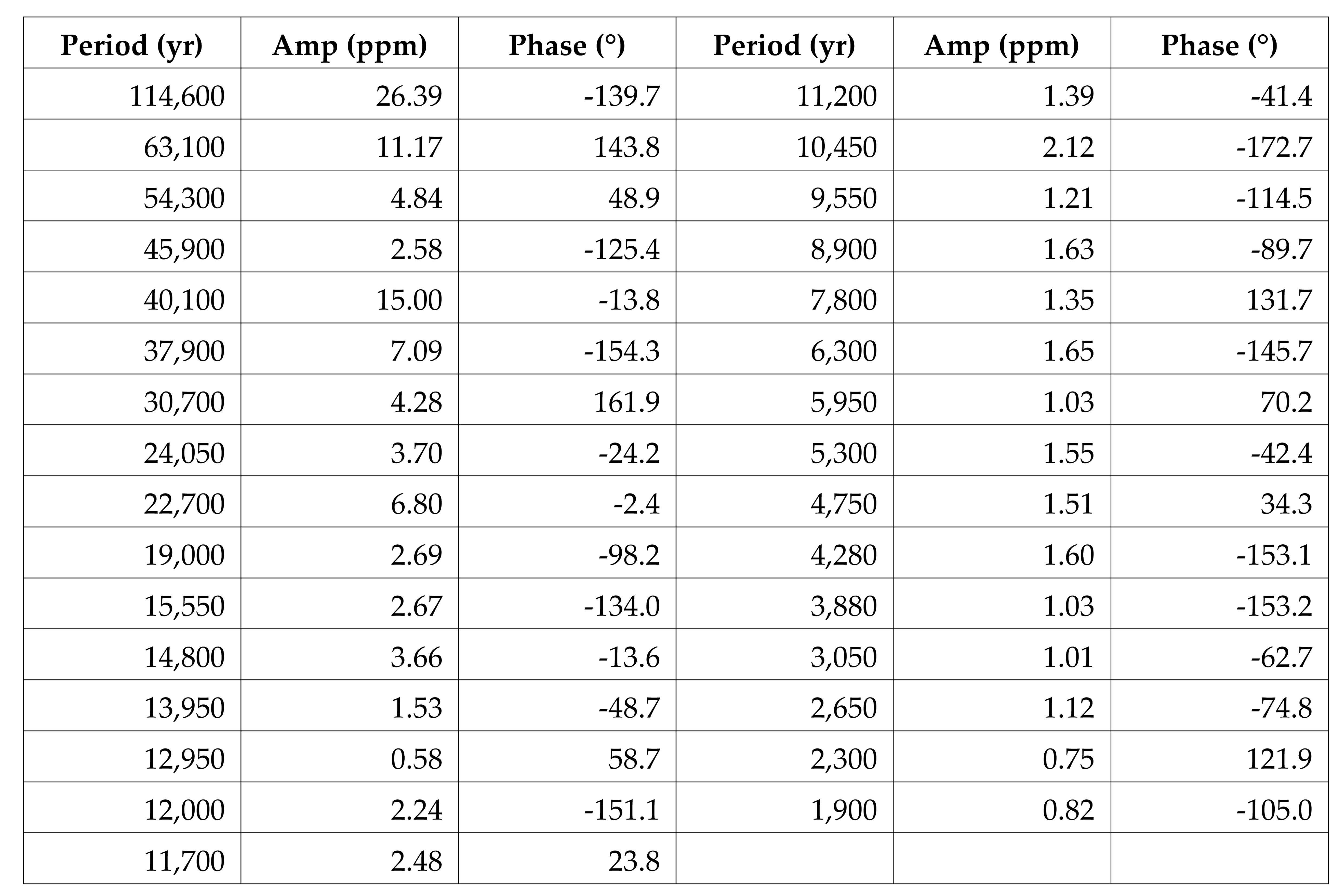
The CO2 fit found by the greedy algorithm followed by pruning to minimize off diagonal correlation, achieves R2 = 0.958 using a constant and 31 periods. The maximum off diagonal correlation is 0.47.
3.8. CH4 Fit with Periods from Greedy Algorithm
This independent recovery validates both the methodology and the orbital pacing hypothesis for glacial-interglacial cycles.
The greedy algorithm independently recovered orbital periods for all cases:
3.9. Cross Correlation
The fit to temperature was evaluated at 10 year intervals from 350,000 BCE to 1850 CE. Similarly the fit to CO2 by the greedy algorithm with pruning (31 periods and a constant) was similarly evaluated. These time series were cross correlated and the results are shown in Figure 19 .
Cross-correlation was computed as a function of time lag τ, where positive τ represents CO2/CH4 shifted forward relative to temperature – a positive lag. A peak in correlation at negative lag indicates that the second variable (CO2 or CH4) follows temperature; a peak at positive lag would indicate the reverse. The correlation values shown are negative because the fits were evaluated relative to their respective means, and both gases increase with warming (positive correlation with temperature change from the mean).
Similarly the fit to CH4 was evaluated and cross correlated with temperature. For all cases plotted, CH4 shows a lag with respect to temperature.
The consistency of the lag for CH4 indicates that the time series agree on registration of their respective quantity with time. This suggests that the changing lag associated with the CO2 plot is either real or the time registration of the CO2 quantity has an error.
3.10. Cross Plots
The time series used for the correlations of section 3.9 were used to generate cross plots. The cross plot for CO2 indicates a curvature that tends toward flattening with higher temperature. This may have an influence on the asymmetry discussed in section 3.5. The CH4 cross plot shows a linear trend. High temperatures are associated with the relatively narrow interglacial peaks. This limits the data available at high temperatures in these plots.
This saturation behavior of CO2 is consistent with temperature-dependent ocean solubility, where the capacity for CO2 release diminishes as the ocean warms.
4. Discussion
4.1. Temperature Drives CO2 at Orbital Timescales
The consistent lag of CO2 behind temperature at orbital periods, for fits using the same periods, is evidence that temperature drives CO2, not the reverse. Both variables fit with R2 > 0.95 using identical periods, with CO2 systematically lagging. This supports: (1) orbital forcing modulates insolation; (2) temperature responds; (3) CO2 responds to temperature through ocean degassing, circulation changes, and terrestrial carbon storage. These findings are consistent with previous phase analyses (Humlum et al., 2013; Grabyan, 2025).
The independent recovery of Milankovitch periods by the greedy algorithm, without prior specification, provides strong validation that these signals are genuine features of the data rather than artifacts of the fitting procedure. The consistency across temperature, CO2, and CH4 records further supports the orbital pacing hypothesis.
4.2. Mechanisms for Asymmetric Response
Atmospheric Transport Limitation: During warming, dissolved CO2 is immediately available for release at the air-sea interface. During cooling, atmospheric CO2 must find its way back to the ocean surface—a rate-limited process.
Plant Stress Feedback: As CO2 declines, C3 vegetation becomes stressed near 200 ppm, reducing uptake and creating a floor below which CO2 cannot easily fall.
Sea Ice Expansion: Growing sea ice caps the ocean surface, reducing gas exchange area precisely when cooling is most rapid.
4.3. The Modern CO2 Anomaly
The fit extrapolated beyond the data shows gentle Holocene oscillation around 270–280 ppm. Actual CO2 departing above 350 ppm after ~1850 CE lies far outside the orbital envelope. This analysis establishes the baseline from natural forcing; whatever drives modern CO2, it is not the orbital mechanics governing the past 350,000 years.
5. Conclusions
1. Greedy harmonic analysis fits Antarctic ice core temperature, CO2 and CH4 over 350,000 years with R2 > 0.95, independently recovering Milankovitch periods (Milankovitch, 1941). Covariance matrix analysis guided refinement of the temperature fit, in particular, from 59 to 55 periods, ensuring stable parameter estimates.The refinement from 59 to 55 periods eliminated all correlations exceeding |r| = 0.50, reducing the maximum from 0.95 to 0.15 for temperature.
2. CO2 lags temperature by 600–4,000 years at orbital timescales, supporting temperature-driven carbon cycle dynamics. This conclusion is based on phase analysis shown in Table 2 section 3.4. However the formal standard error computation indicates large possible errors. This conclusion is based primarily on consistency for eccentricity and Obliquity. Cross- correlation of temperature and CO2 shows CO2 lagging temperature when applied to the full ~352,000 years of input data. However as data is clipped toward recent time the lag shifts to a lead for CO2. For CH4 the cross-correlation consistently indicates that CH4 lags temperature.
3. The Eemian shows CO2 elevated for ~13,000 years while temperature fell ~7°C, indicating asymmetric absorption/release kinetics. This asymmetric behavior may be the reason direct comparison of phase is difficult.
4. The modern CO2 spike is anomalous relative to the 350,000-year orbital pattern – obvious for all existing ice-core data.
5. The Younger Dryas temperature event is fit quite well as can be seen in Figure 4. The fit involves 111 fit parameters but this corresponds to roughly one parameter every 3000 years which seems quite reasonable for the observed accuracy of the fit, especially given the normalized covariance indication of little correlation between periods. The Younger Dryas event is even more prominent in the CH4 data and is harder to fit but it is reasonably well represented as shown in Figure 18.
6. The R squared analysis shown in Figure 10 appears to unambiguously find the Mid-Pleistocene Transition and clearly justifies limiting the fit to the interval chosen.
Funding
No external funding was received for this research.
Conflicts of interest
The author declares no conflicts of interest.
Appendix A: Fit Statistics for the Case Where Both Fits Involved the Same Periods
A.1 Temperature Fit (55 Periods)
- R2 = 0.95168
- Time range: 1911 CE to −350,245 years
- Origin: t0 = −175,000 years
- Constant: C = −5.59°C
- Data points: 4,752
- Periods removed: 22,150 / 9,000 / 8,000 / 4,540 years
A.2 CO2 Fit (55 Periods, Truncated at 1850 CE)
- R2 = 0.96418
- Time range: 1851 CE to −351,225 years
- Origin: t0 = −175,000 years
- Constant: C = 225.5 ppm
A.3 Covariance Matrix Interpretation
The covariance matrix Σ for a least-squares fit contains parameter variances on the diagonal (σ2) and covariances off-diagonal. The normalized covariance (correlation) matrix has elements rᵢⱼ = Σᵢⱼ / √(Σᵢᵢ Σⱼⱼ), ranging from −1 to +1. Values |r| > 0.5 indicate substantial correlation requiring attention; |r| > 0.9 indicates near-collinearity where parameters cannot be independently estimated. The refinement from 59 to 55 periods eliminated all correlations exceeding |r| = 0.50, reducing the maximum from 0.95 to 0.15 for temperature.
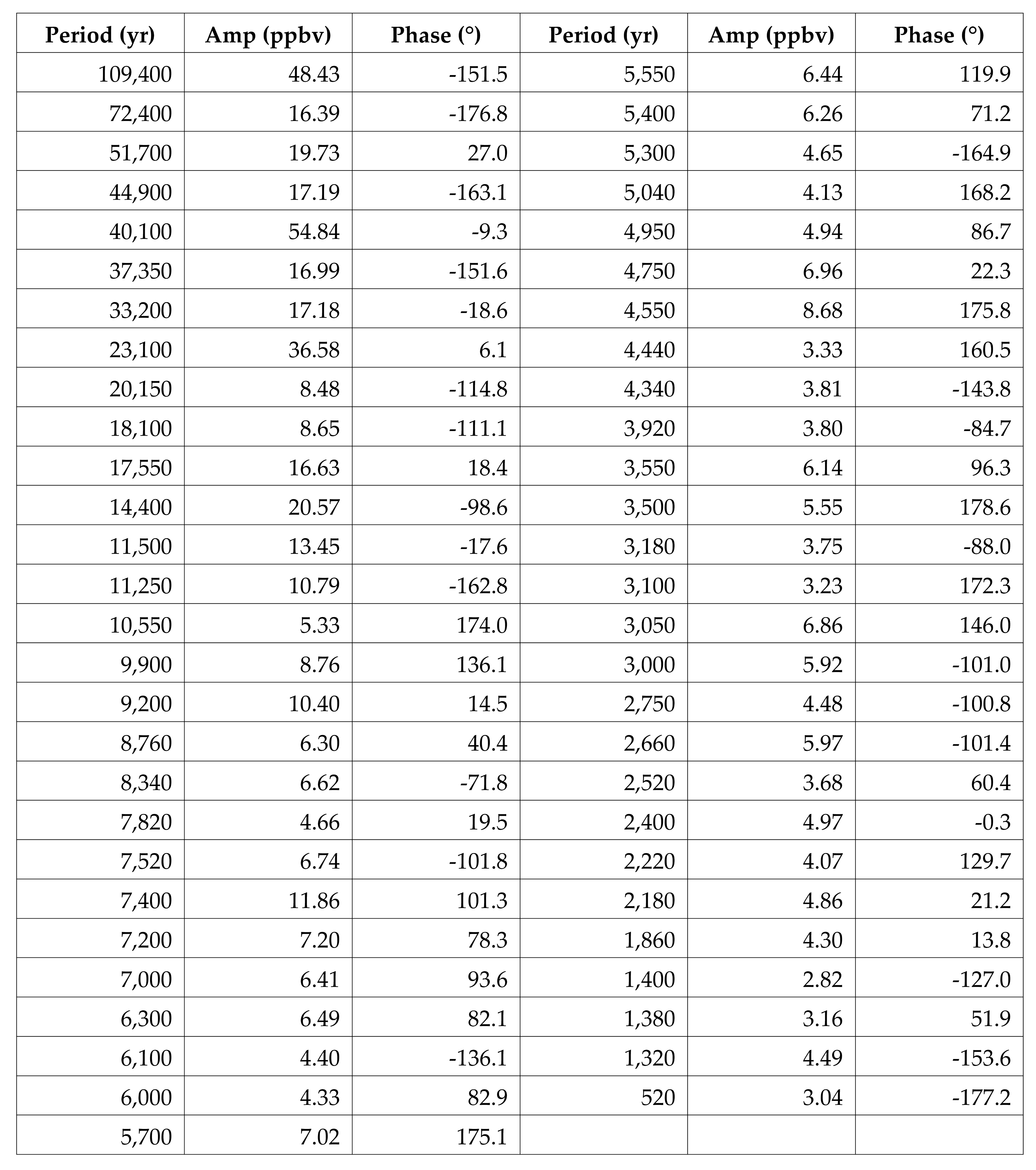
Appendix B: Temperature Fit Parameters (55 Periods)
Amplitude units: °C. Phase normalized to positive amplitude convention.
Appendix C: CO2 Fit Parameters for Periods from Temperature Fit (55 Periods)
Amplitude units: ppm. Phase normalized to positive amplitude convention.
Appendix D: Phase Lag Methodology
D.1 Phase Normalization Convention
The least-squares fit can return either sign for amplitude. A negative amplitude A with phase φ is mathematically equivalent to positive amplitude |A| with phase φ + 180°. To ensure consistent comparison, all amplitudes are normalized to positive by adding 180° to the phase when the fitted amplitude was negative.
D.2 Lag Calculation
Phase difference: Δφ = φ_CO2 − φ_Temperature, wrapped to ±180°.
Time lag: τ = (Δφ / 360°) × P, where P is the period.
Negative τ indicates CO2 lagging temperature; positive τ indicates CO2 leading.
D.3 Uncertainty Notes
The large formal uncertainties on phase lags (often comparable to or exceeding the lag values) reflect the inherent difficulty of precisely determining phases in a multi-period harmonic decomposition. However, the consistent sign pattern across multiple periods—with the three major Milankovitch cycles all showing CO2 lagging—provides stronger evidence than any individual period, as the probability of this occurring by chance under a null hypothesis of zero lag is small.
Appendix E: Complete Phase Lag Analysis (55 Periods)
Phase lag between temperature and CO2 fits for all 55 periods, sorted by period (descending). Negative lag indicates CO2 lagging temperature; positive indicates CO2 leading.
Summary: 30 periods show CO2 lagging (negative lag), 25 periods show CO2 leading (positive lag). Mean lag = −523 years.
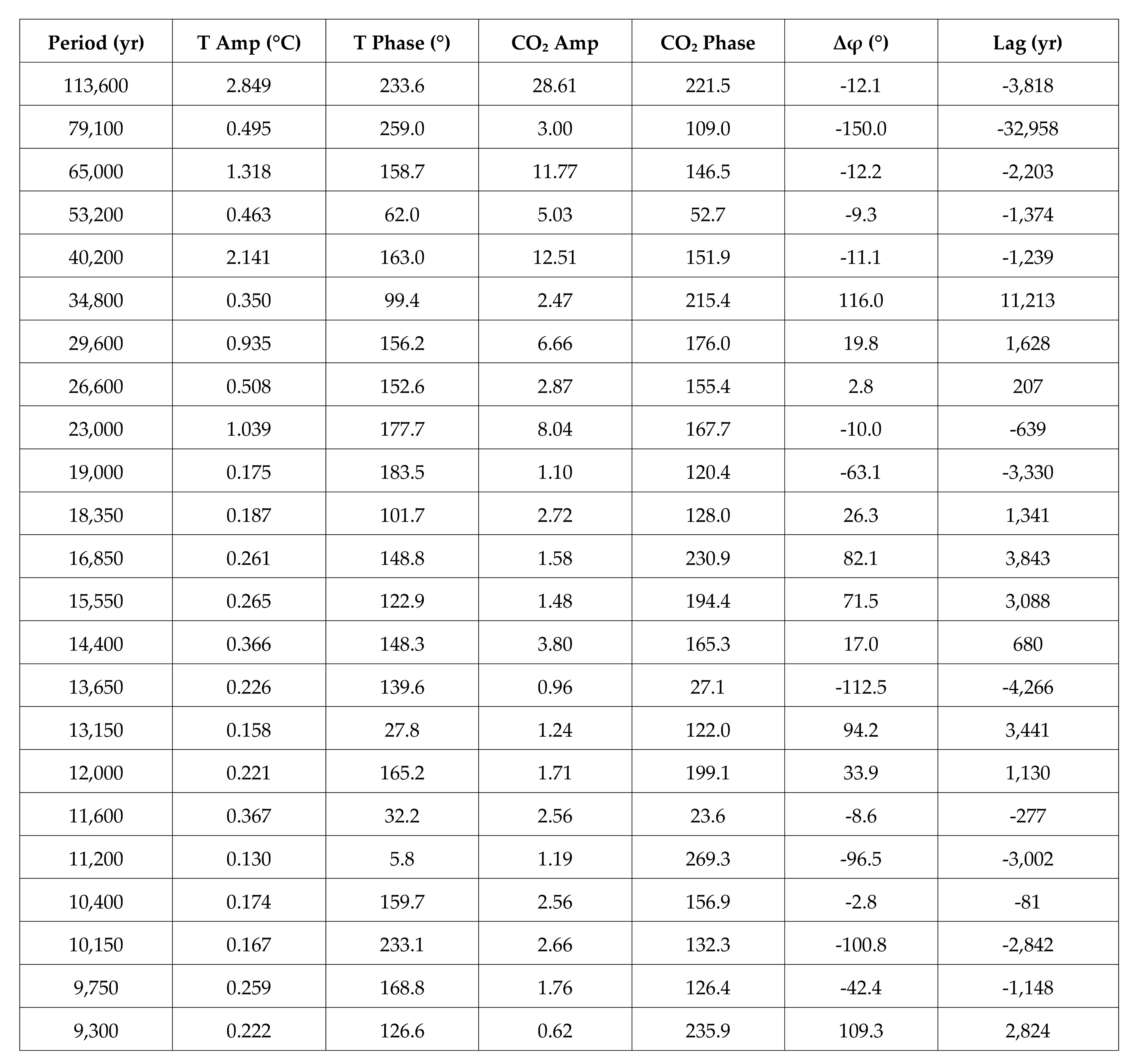
Table E1.
(continued): Periods 8,900 to 1,460 years.
| Period (yr) | T Amp (°C) | T Phase (°) | CO2 Amp | CO2 Phase | Δφ (°) | Lag (yr) |
|---|---|---|---|---|---|---|
| 8,900 | 0.142 | 212.7 | 1.31 | 248.9 | 36.2 | 895 |
| 8,180 | 0.127 | 119.3 | 0.48 | 230.8 | 111.5 | 2,534 |
| 7,900 | 0.145 | 138.0 | 1.47 | 177.9 | 39.9 | 876 |
| 7,600 | 0.234 | 169.7 | 2.01 | 135.3 | -34.4 | -726 |
| 7,050 | 0.176 | 179.9 | 1.46 | 216.7 | 36.8 | 721 |
| 6,400 | 0.135 | 108.4 | 0.84 | 117.4 | 9.0 | 160 |
| 6,160 | 0.087 | 147.3 | 2.02 | 11.1 | -136.2 | -2,331 |
| 5,950 | 0.158 | 163.7 | 1.18 | 123.9 | -39.8 | -658 |
| 5,900 | 0.110 | 27.8 | 2.18 | 86.5 | 58.7 | 962 |
| 5,650 | 0.124 | 127.6 | 0.93 | 125.8 | -1.8 | -28 |
| 5,560 | 0.096 | 113.8 | 0.88 | 79.5 | -34.3 | -530 |
| 5,400 | 0.238 | 117.6 | 0.86 | 100.2 | -17.4 | -261 |
| 5,280 | 0.132 | 240.7 | 1.08 | 136.0 | -104.7 | -1,536 |
| 5,100 | 0.084 | 116.2 | 1.06 | 215.7 | 99.5 | 1,410 |
| 4,940 | 0.079 | 116.7 | 1.04 | 216.5 | 99.8 | 1,369 |
| 4,880 | 0.098 | 151.9 | 0.85 | 139.1 | -12.8 | -174 |
| 4,800 | 0.092 | 123.2 | 1.03 | 52.7 | -70.5 | -940 |
| 4,550 | 0.181 | 241.1 | 0.73 | 268.9 | 27.8 | 351 |
| 4,320 | 0.103 | 122.7 | 1.44 | 124.0 | 1.3 | 16 |
| 3,980 | 0.130 | 194.4 | 0.73 | 132.4 | -62.0 | -685 |
| 3,950 | 0.111 | 55.2 | 1.15 | 84.1 | 28.9 | 317 |
| 3,550 | 0.121 | 152.0 | 0.21 | 33.0 | -119.0 | -1,173 |
| 3,380 | 0.065 | 257.7 | 0.66 | 93.3 | -164.4 | -1,544 |
| 3,280 | 0.078 | 125.8 | 0.42 | 190.5 | 64.7 | 589 |
| 3,200 | 0.070 | 248.7 | 0.87 | 15.1 | 126.4 | 1,124 |
| 3,160 | 0.112 | 264.0 | 0.41 | 154.3 | -109.7 | -963 |
| 3,040 | 0.110 | 158.7 | 0.40 | 247.3 | 88.6 | 748 |
| 2,960 | 0.098 | 149.9 | 0.26 | 142.9 | -7.0 | -58 |
| 2,580 | 0.079 | 114.8 | 0.27 | 11.7 | -103.1 | -739 |
| 2,520 | 0.074 | 157.5 | 0.59 | 170.1 | 12.6 | 88 |
| 1,980 | 0.065 | 240.6 | 0.44 | 128.6 | -112.0 | -616 |
| 1,460 | 0.069 | 165.2 | 0.79 | 125.2 | -40.0 | -162 |
E.1 Notes on Interpretation
The 79,100-year period shows an anomalously large negative lag (−32,958 years), which wraps around to effectively represent a phase difference near 150°. This period has relatively small temperature amplitude (0.495°C) and probably represents a combination tone or harmonic rather than a primary orbital signal. Similarly, periods showing very large positive lags (e.g., 34,800 yr at +11,213 yr) likely reflect phase wrapping artifacts where the "true" lag interpretation is ambiguous.
The most physically meaningful phase relationships are found at the three major Milankovitch periods (113,600, 40,200, and 23,000 years), which have the largest amplitudes in both temperature and CO2 and show consistent CO2 lags of 640–3,800 years. These periods correspond to well-understood orbital mechanics and provide the strongest constraints on the temperature-CO2 phase relationship.
Appendix F: CO2 Fit Parameters (31 Periods)
Amplitude units: ppm. Phase normalized to positive amplitude convention.
R2 = 0.958, Constant = 225.74 ppm, Max |r| = 0.47
Covariance Matrix Notes:
• The normalized covariance matrix was computed to verify conditioning
• Periods were iteratively added until R2 > 0.95 achieved
• Four periods removed during pruning to reduce max |r| below 0.50
• Final basis shows acceptable independence between components
Appendix G: CH4 Fit Parameters (55 Periods)
Amplitude units: ppbv. Phase normalized to positive amplitude convention.
R2 = 0.873, Constant = 485.84 ppbv, Max |r| = 0.40
Covariance Matrix Notes:
• CH4 record shows higher intrinsic variability than CO2
• More periods required to capture millennial-scale variations
• Lower R2 reflects noisier data rather than inadequate model
• Maximum correlation |r| = 0.40 indicates well-conditioned basis
References
- Bereiter, B.; Eggleston, S.; Schmitt, J.; Nehrbass-Ahles, C.; Stocker, T.F.; Fischer, H.; Kipfstuhl, S.; Chappellaz, J. Revision of the EPICA Dome C CO2 record from 800 to 600 kyr before present. Geophysical Research Letters 2015, 42, 542–549. [Google Scholar] [CrossRef]
- Berends, C.J.; Köhler, P.; Lourens, L.J.; van de Wal, R.S.W. On the Cause of the Mid-Pleistocene Transition. Reviews of Geophysics 2021, 59, e2020RG000727. [Google Scholar] [CrossRef]
- Clark, P.U.; Archer, D.; Pollard, D.; Blum, J.D.; Rial, J.A.; Brovkin, V.; Mix, A.C.; Pisias, N.G.; Roy, M. The middle Pleistocene transition: Characteristics, mechanisms, and implications for long-term changes in atmospheric pCO2. Quaternary Science Reviews 2006, 25, 3150–3184. [Google Scholar] [CrossRef]
- Grabyan, R. Global Atmospheric CO2 Lags Temperature: Implications for Short- and Long-Term Climate Predictions. Science of Climate Change 2025, 5(3), 302–326. [Google Scholar]
- Higginbotham, J. Planetary Orbits and Sea-Level During the Phanerozoic: Correlation, Causation, and Forecasting. Journal of Biomedical Research & Environmental Sciences 2025, 6(4), 926–940. [Google Scholar]
- Humlum, O.; Stordahl, K.; Solheim, J.E. The phase relation between atmospheric carbon dioxide and global temperature. Global and Planetary Change 2013, 100, 51–69. [Google Scholar] [CrossRef]
- Jouzel, J. Orbital and Millennial Antarctic Climate Variability over the Past 800,000 Years. Science 2007, 317(5839), 793–796. [Google Scholar] [CrossRef] [PubMed]
- Loulergue, L.; Schilt, A.; Spahni, R.; Masson-Delmotte, V.; Blunier, T.; Lemieux, B.; Barnola, J.-M.; Raynaud, D.; Stocker, T.F.; Chappellaz, J. Orbital and millennial-scale features of atmospheric CH4 over the past 800,000 years. Nature 2008, 453, 383–386. [Google Scholar] [CrossRef] [PubMed]
- Milankovitch, M. Kanon der Erdbestrahlung und seine Anwendung auf das Eiszeitenproblem; Royal Serbian Academy Special Publication 133: Belgrade, 1941. [Google Scholar]
Figure 9.
Here the full Temperature proxy data set was fit with the same 55 periods found by the temperature fit and a constant. The fit from date -400,000 to 1911 is fit reasonably well but the deviations for dates prior to date -400,000 are large. This is consistent with the MPT.
Figure 9.
Here the full Temperature proxy data set was fit with the same 55 periods found by the temperature fit and a constant. The fit from date -400,000 to 1911 is fit reasonably well but the deviations for dates prior to date -400,000 are large. This is consistent with the MPT.
Disclaimer/Publisher’s Note: The statements, opinions and data contained in all publications are solely those of the individual author(s) and contributor(s) and not of MDPI and/or the editor(s). MDPI and/or the editor(s) disclaim responsibility for any injury to people or property resulting from any ideas, methods, instructions or products referred to in the content. |
© 2025 by the author. Licensee MDPI, Basel, Switzerland. This article is an open access article distributed under the terms and conditions of the Creative Commons Attribution (CC BY) license (https://creativecommons.org/licenses/by/4.0/).
Copyright: This open access article is published under a Creative Commons CC BY 4.0 license, which permit the free download, distribution, and reuse, provided that the author and preprint are cited in any reuse.


