
Submitted:
22 April 2025
Posted:
23 April 2025
You are already at the latest version
Abstract
The theory of orbital forcing as formulated by Milankovitch involves the mediation by the ad-vance (retreat) of ice sheets and the resulting variations in terrestrial albedo. This approach poses a major problem, that of the period of glacial cycles which varies over time as happened during the Mid-Pleistocene Transition (MPT). Here, we show that various hypotheses are called into question because of the finding of a second transition, the Early Quaternary Transition (EQT) resulting from the million-year period eccentricity parameter. We propose to complement the orbital forcing theory to explain both the MPT and the EQT by invoking the mediation of western boundary currents (WBCs) and the resulting variations in heat transfer from the low to the high latitudes. From observational and theoretical considerations, it appears that very long period Rossby waves winding around subtropical gyres, the so-called “gyral” Rossby waves (GRWs), are resonantly forced in subharmonic modes from variations in solar irradiance resulting from the solar and orbital cycles. Two mutually reinforcing positive feedbacks of the climate response to orbital forcing have been evidenced, namely the change in the albedo resulting from the cyclic growth and retreat of ice sheets in accordance with the standard Milankovitch theory, and the modulation of the velocity of the WBCs of subtropical gyres. Due to the inherited resonance properties of GRWs, the response of the climate system to orbital forcing is sensitive to small changes in the forcing periods. For both the MPT and the EQT, the transition occurred when the forcing period merged with one of the natural periods of the climate system. The MPT occurred 1.25 Ma ago when the dominant period shifted from 41 ka to 98 ka, with both periods corresponding to changes in the Earth's obliquity and eccentricity. The EQT occurred 2.38 Ma ago when the dominant period shifted from 408 ka to 786 ka, with both periods corresponding to changes in the Earth's eccentricity. Through this paradigm shift, the objective of this article is essentially to spark new debates around a problem that has been pending since the discovery of glacial-interglacial cycles, where many hypotheses have been put forward without, however, fully answering all our questions.
Keywords:
ice sheet
; Mid-Pleistocene Transition
; subharmonic modes
; Long-period Ocean Rossby Waves
; Quaternary
; subtropical gyres
; Western Boundary Currents
1. Introduction
Since Milankovitch's work, that variations in solar irradiance at certain latitudes and seasons are responsible for the growth and retreat of ice sheets with induced variations in the earth's albedo, observations from climate records have shown shortcomings in the theory of orbital forcing. Indeed, the orbital forcing resulting from obliquity should prevail over eccentricity. This is due to the magnitude of the variation in solar irradiance, especially in the high latitude regions of the Earth's north during the summer. Milankovitch calculated that ice ages occur approximately every 41 ka. Since then, various observations have confirmed that they occurred at 41 ka intervals between one and three million years. But about 1.2 Ma ago, the cycle of ice ages lengthened to 100 ka, corresponding to the cycle of eccentricity of the Earth. The Milankovitch theory has proved unable to explain the 100-ka cycle from orbital forcing [1], which became known as the "100 ka problem" [2].
1.1. The Mid-Pleistocene Transition (MPT)
1.1.1. The Observations
The discovery of the Mid-Pleistocene Transition (MPT), that is a fundamental change in the behavior of glacial cycles during the Quaternary glaciations, is the result of observations of foraminifera in sediment cores, that is, benthic δ18O records. The series obtained from 57 globally distributed sites [3], what is named the ‘‘LR04’’ stack, highlights the variations in the Earth's average temperature over the past 5.3 Ma. This synthesis shows with a remarkable resolution the oscillations of the temperature subject to orbital forcing. The influence of orbital forcing on global temperature observed from proxy records was confirmed following the publication of a seminal paper by Hays, Imbrie and Shackleton [4], before further evidence was provided [5,6].
MPT occurred nearly 1.25 million years ago, during the Pleistocene. Prior to MPT, the mean period of glacial cycles was 41 ka, consistent with orbital forcing due to axial tilt (Figure 1). After the MPT, the period increased around 100 ka, exhibiting a sawtooth pattern (gradual growth and rapid termination), consistent with orbital forcing due to eccentricity. However, the intensity of forcing resulting from eccentricity is much lower than that induced by axial tilt.
1.1.2. Hypotheses Are Based on the Coevolution of Climate and Ice Sheets
A natural resonance frequency of 100 ka resulting from feedback processes within the Earth's climate system has been hypothesized, but without proposing a plausible physical mechanism [9,10]. A master-slave synchronization between the natural frequencies of the climate system and the forcing resulting from eccentricity has been propounded, which triggered the 100 ka ice ages of the late Pleistocene with large amplitude [11]. Here again, it remained to find internal climatic feedback that may be at work.
- One or two thresholds control ice-sheet stability.
Most of the physical mechanisms invoked to explain the modification of the response to orbital forcing, which is assumed to be immutable, include various nonlinear feedbacks. These involve ice sheets and the carbon cycle inducing a slow and steady cooling trend throughout the Pleistocene. Many ice-sheet-climate feedbacks mechanisms rely on the existence of one or two thresholds that control ice-sheet stability during the Pleistocene [12,13,14,15,16,17,18].
Berends et al. [18] propose that the sensitivity of an ice sheet to changes in insolation depends on its size. More specifically, the response of the ice sheet is divided into three regimes, the passage from one to the other being governed by thresholds. An ice sheet that is too small in size cannot survive an insolation maximum, which leads to the almost linear response of ice volume to variations in insolation of period 41 ka during the Lower Pleistocene [13,19]. Above a certain size, the ice-albedo and elevation-temperature feedbacks allow the ice sheet to survive an insolation maximum. Above a greater size, the bedrock-mass-balance feedback and calving lead to the ice sheet becoming unstable. An insolation maximum will then trigger a self-sustained retreat, leading to the rapid vanishing of the ice sheet.
The existence of the first threshold that separates small ice sheets with linear-response to solar irradiance, from medium-sized ice sheets, less sensitive to external forcing, is well supported by the various model studies [12,20,21]. Indeed, ice-albedo and altitude-temperature feedbacks are well established in the literature and have been shown to lead to such a threshold. The physical mechanisms underlying the second threshold, above which ice sheet sensitivity increases sharply, is more uncertain. The magnitude of their effects is difficult to quantify.
From [22] the ocean is the intermediary of the orbital forcing of the ice sheet. The ocean is assumed to be inherently turbulent and tends toward maximum entropy production, which makes the ice sheet bistable. Since the bistable frequency is lowered during Pleistocene cooling, the ice-albedo feedback could explain the mid-Pleistocene transition.
- Long-term changes in atmospheric CO2.
Works based on the dynamics of ice sheets [23,24] may include long-term changes in atmospheric CO2 over the Quaternary [25,26,27,28,29]. Insolation and internal feedbacks involving the ice sheets and the lithosphere-asthenosphere system may explain the 100-ka periodicity [12]. For this, the authors argue that the larger the ice sheet grows and extends towards lower latitudes, the smaller the insolation required to make the mass balance negative. An almost complete retreat of the ice sheet is favored by the lowered surface elevation resulting from delayed isostatic rebound, which makes the ice sheet more vulnerable to melting. Carbon dioxide is involved but is not determinative in the adjustment of the natural frequency. By supposing no change in orbital forcing over the past million years, these assumptions are all based on the properties of the ice sheets in the Northern Hemisphere linked to the gradual cooling during the Pleistocene [13,14,29,30,31,32].
From [25] the forcings are both insolation and CO2 concentration. By using a linearly decreasing CO2 concentration going from 320 ppmv at 3 Ma to 200 ppmv at present, nearly before 1 Ma the dominating period is about 41 ka, then the ∼100 ka period becomes dominant. From [13] is emphasized the importance of ice dynamics and ice–climate interactions in controlling the 100 ka glacial cycles. This is based on the temporal changes in air temperature and ice volume, with enhanced North American ice-sheet growth and the following merging of the ice sheets. According to [30] the gradual cooling of the deep ocean during the Pleistocene leads to the initiation of the 100-ka oscillations. Gradual glaciation and rapid deglaciations occur because the mean value of the ice sheet ablation is close to the maximum rate of snow accumulation during warm periods.
- Gradual erosion of high-latitude northern hemisphere regolith.
Some papers are based on gradual erosion of high-latitude northern hemisphere regolith by multiple cycles of glaciation, which would have caused a transition in ice sheet response to external forcing. From [14] the Laurentide ice sheet is controlled by glacial erosion of a thick regolith and the resulting exposure of unweathered bedrock. From [31] 100-ka periodicity in the ice volume variations and the timing of glacial terminations during past 800 ka result from strongly nonlinear responses of the climate-cryosphere system to orbital forcing. This supposes that the atmospheric CO2 concentration stays below its typical interglacial value. The 100-ka cycle is primarily attributed to the North American ice sheet and requires the presence of a large continental area with exposed rocks. From [32] the “regolith hypothesis” is strengthened by supposing a combination of climate and ice-flow changes, with crystalline bedrock producing thicker, colder ice sheets that accumulate more snowfall and have a smaller ablation zone. Willeit et al. [29] used a coupled ice-sheet – climate – carbon cycle model, forced with orbital cycles. The co-evolution of climate and the arctic ice sheet over the last 3 million years implies a decrease in atmospheric carbon dioxide content as well as a progressive elimination of regoliths during the Quaternary.
- Certain insolation peaks are ‘skipped’.
Presently, a predominant view is that eccentricity is not the driver of the 100-ka cycle that rather reflects integer multiples of the 41-ka obliquity cycle (82/123 ka) or the ∼20 ka precession cycle (80/100/120 ka), e.g. [33,34,35,36]. From [35] interglacial occurs when the energy related to summer insolation exceeds a threshold, about every 41 ka. Larger ice sheets over the past million years are a consequence of an increase in the number of skipped insolation peaks. From [36], before the MPT, obliquity alone was enough to end a glacial cycle, before losing its influence on deglaciation since ~1 Ma. This is attributed to the southward extension of the north hemisphere's ice sheets. According to the MPT, a combination of obliquity and precession cycles is required to initiate deglaciation. The two-threshold model [18] supposes that all terminations are caused by insolation maxima that occur every 41 ka, but not all insolation maxima cause terminations so that the duration of glacial cycles can vary arbitrarily between 82 and 123 ka. This hypothesis will be challenged when results are presented showing that the period of orbital forcing resulting from obliquity has varied little over the last 2.5 million years. These small variations cannot explain the MPT without invoking the resonant forcing of the climate response.
1.2. In Search of a Unified Explanation of Climate Transitions
The hypotheses based on the determining role of the dynamics of growth and retreat of the ice sheets in tuning the natural frequency of the climate system to 100 ka suffer from arbitrary assumptions to justify the precise timing of the transition. Conditions which make the ice sheets insensitive to variations in insolation resulting from the precession and the obliquity of the earth, but sensitive to the eccentricity, have to be hypothesized, which supposes an opportune adjustment of the Earth system to explain what is observed [29].
Facing this challenging puzzle, machine learning approaches has been used to disclose the main mechanisms underlying Pleistocene variability, with the aim of explaining proxy records and testing existing theories [37]. With a similar idea, a dynamical ramping mechanism with frequency locking has been used, assuming an interaction between the internal period of a self-sustained oscillator and forcing that contains periodic components [38,39]. Such approaches relying on conceptual mechanisms with frequency locking did not bring anything concrete on the physical phenomena involved. But they show the need to search for a physical basis for the resonant forcing of the climate system.
By testing competing forms of the Milankovitch hypothesis from a multivariate approach, it has been shown that the climate variables are driven partly by solar insolation, determining the timing and magnitude of glaciations and terminations, and partly by internal feedback dynamics, pushing the climate variables away from equilibrium [40]. The authors argue that the Milankovitch hypothesis should be restated as follows: “internal climate dynamics impose perturbations on glacial cycles that are driven by solar insolation and, from adjustment dynamics, that solar insolation affects an array of climate variables other than ice volume, each at a unique rate.”
1.3. The Milankovitch Theory Revisited
Returning to the theory of orbital forcing stricto sensu, here, we propose to fill a gap. The sole mediation by ice sheets of the response of the climate system to orbital forcing cannot explain a phenomenon, the MPT, which presents resonance characteristics. This insufficiency will become even more blatant when we highlight a second transition, the Early Quaternary Transition (EQT). The search for a complementary mediator leads to ocean subtropical gyres which cause the climate system to be subject to resonant orbital forcing. The method we will use to explain both transitions consists of taking advantage of very long-period Rossby waves winding around subtropical gyres, the so-called Gyral Rossby Waves (GRWs) which have the property of resonating in subharmonic modes under the effect of orbital forcing [41,42,43]. Their climatic impact is considerable because they control heat transfers from low to high latitudes depending on whether the acceleration of the western boundary current (WBC), west of the ocean gyre circulation, occurs poleward or equatorward. New hypotheses will be advanced about feedback on the climate involving both sea ice and WBCs so that the climate sensitivity to orbital forcing depends on the deviation between the forcing period and the nearest natural period of the climate system.
2. Method
2.1. Dynamics of Oceanic Subtropical Gyres
As indicated in the introduction, the innovative character of this research lies in considering the key role played by the WBCs in climate variability and, more particularly, in the properties of Rossby waves guided by the WBCs. In the northern hemisphere they are observed in the western basins of the Atlantic and Pacific subtropical gyres, that is, regions of intense WBCs: the Gulf Stream and the Kuroshio [44,45,46,47]. The mass input into the western boundary region is accurately described by the jet-trapped Rossby wave framework. Historically it was thought that Rossby waves govern the formation of warm-core anticyclonic eddies shed from the East Australian Current jet, that is, the WBC associated with the South Pacific subtropical gyre [48,49,50]. These pioneering works highlight the key role in mass and heat transfer of short-period Rossby waves driven in WBCs.
Long-period Rossby waves have been demonstrated from a weakly damped mode of variability in the North Atlantic, corresponding to the oceanic signature of the Atlantic multidecadal oscillation (AMO) [51]. This results from a westward propagation of density anomalies in the pycnocline, typical of large-scale baroclinic Rossby waves. This mode is described in four phases composing a complete oscillation cycle. It involves alternately the basin-wide North Atlantic circulation and the Atlantic meridional overturning circulation (AMOC) along the North Atlantic Current after bifurcation of the Gulf Stream to the north: 1) basin-scale warming of the North Atlantic (AMO positive phase), 2) reduction of the AMOC, 3) basin-scale cooling (negative AMO), and 4) AMOC intensification.
Examination of the latest unforced CMIP6 simulations in the study of Eurasia winter temperature unveils a significant contribution of the AMO’s thermodynamic effects, resulting in warm (cold) phases during positive (negative) AMO cycles, along with increased (decreased) warm extremes and reduced (enhanced) cold extremes [52]. More generally, the AMO is a global-scale coupled ocean-atmosphere oscillation of the climate system with significant sea surface temperature (SST) anomalies in all ocean basins [53].
These works report the omnipresence of Rossby waves guided by WBCs, but also of long-period Rossby waves which impact the North Atlantic circulation on a basin-scale, the average period of which revealed by the AMO is nearly 64 years. Other observations based on the frequency analysis of SST anomalies over the global ocean highlight Rossby waves with a mean period of 64 or 128 years around the 5 subtropical gyres [42].
1/2-, 1-, 4- and 8-year period Rossby waves highlighted from Sea Surface Height (SSH) anomalies are confined to the west of the gyres with a maximum amplitude where the WBCs leave the continents. They extend further towards the east of the gyre as their period increases. As for the long-period Rossby waves, they are highlighted by an SST anomaly around the gyre as well as an SST anomaly outside the gyre towards the pole (the AMOC in the North Atlantic), these two anomalies being in phase opposition. These observations highlight the superposition of multi-frequency Rossby waves, mainly where the WBCs leave the continents to re-enter the subtropical gyres, but also around the gyres.
2.2. The Annular Representation of Long-Period Rossby Waves
Very long-period Rossby waves have the property of winding around themselves around the 5 subtropical gyres. The justification for the existence of such waves results from both an observational and theoretical approach.
2.2.1. Observation of a 64-Year Period Rossby Wave Around the North Atlantic Gyre
The observation of GRWs can be conducted from the analysis of the SST over a long period of time. Indeed, direct observation of these waves from their geostrophic currents or from sea surface perturbations is not possible because these data have only been known since the early 1990s. On the other hand, SST has been known since the beginning of the 1850s. This is what allows highlighting long-period Rossby waves from SST anomalies according to the oscillation of the thermocline, based on the amplitude (square root of the power spectrum of the wave) of SST in certain period ranges [42]. However, these results are questionable, due to the lack of reliability of the data from the time, as well as the method adopted to highlight the Rossby wave.
The monthly global (2°×2°) Extended Reconstructed Sea Surface Temperature (ERSST) has been revised and updated from version 4 to version 5 [54]. Highly reliable data provided by NOAA (National Oceanic and Atmospheric Administration) are now available since 1854 [55]. On the other hand, the use of the SST anomaly amplitude in [42] suffers from significant biases due to the rapid cooling of the subsurface waters of the western boundary current as it leaves the continent to re-enter the subtropical gyre, which lowers the sensitivity of the method.
Rather than the amplitude of the SST anomaly, the coherence and the phase of the SST relative to a reference [56] provides more reliable information. Their association specifies the integrity of the wave without any ambiguity. In Figure 2, the coherence and phase of the SST is shown in joint period ranges, whose bandwidth forms a harmonic progression. This clearly highlights the coherence and homogeneity of the phase of quasi-stationary Rossby waves as the period lengthens, which is also true of the apparent wavelength. This construction results in the gyral wave, with a mean period of 64 years (Figure 2i, j).
However, the North Atlantic Gyre appears further north than it should be. This drift in the observed long-term SST anomaly suggests that, as the thermocline lowers due to the influx of warm tropical waters, water vapor resulting from evaporation processes migrates northward to condense and precipitate, providing latent heat to the colder waters. These observations disclose a dominant northward atmospheric flux over the North Atlantic on a multiannual timescale. The northward drift of the SST can be observed and quantified from the 8-year period quasi-stationary wave, as shown in Figure 2k, l. The SST anomaly migrates about ten degrees north of the quasi-stationary wave crest evidenced by the geostrophic zonal current over a period range of 6 to 12 years. Looking at the Figure 2i, j, it turns out that the drift increases at high latitudes of the gyre to reach nearly 20°. However, knowing the origin of the drift, this figure should be considered as reliable evidence for the existence of quasi-stationary oceanic GRWs.
It is not possible to investigate periods longer than 64 years from the SST because the length of the series must be at least three times the period. On the other hand, since gyral waves have a considerable climatic impact, the definition of subharmonic modes beyond 64 years of period can be carried out from the climatic archives by searching for periodicities that are multiples of 64 years.
2.2.2. Theoretical Justification of the Gyral Rossby Waves (GRWs)
Oceanic Rossby waves form where the WBC leaves the continent to re-enter the subtropical gyre. Long-wavelength Rossby waves are approximately non-dispersive. Propagating at the interfaces of stratified media, they owe their origin to the Coriolis parameter β, i.e. the gradient of the Coriolis frequency relative to latitude [57]. As they propagate westward, their phase velocity depends on the latitude. They are embedded in an eastward-propagating background current, so they appear to propagate eastward relative to a fixed referential.
GRWs, as for them, owe their existence to the variation in the Coriolis frequency according to the mean radius of the subtropical gyre in which they are embedded. The transformation of the equations of motion of short-period Rossby waves to GRWs is summarized in the Figure 3, and developed in Appendix A. While the equations of motion for short-period waves are expressed using the β-plane approximation where the Coriolis parameter β is the gradient of the Coriolis frequency with respect to the latitude, the equations of motion for gyral waves are expressed using the β-cone approximation where the Coriolis parameter β is the gradient of the Coriolis frequency with respect to the mean radius of the gyre (the radius of the circle at the intersection of the cone and the sphere that most closely approximates the gyre). With this transformation, the 4 equations of movement of Rossby waves, i.e. the 2 momentum equations, the equation of continuity, and the equation of conservation of the relative vorticity, remain virtually unchanged within the β-cone approximation. It should be noted that the equations governing GRWs apply to short-period waves without transformation when these develop where the western boundary currents leave the continents to re-enter the subtropical gyres.
This is the reason why the properties of the gyral waves expressed in conical coordinates (r, φ, z) deduce from the properties of short periods expressed in Cartesian coordinates (x, y, z). The dispersion relation (A6) of gyral waves is expressed according to the latitude of the centroid of the gyre.
GRWs wind around the subtropical gyre as their period increases, as is their apparent wavelength. Sea surface height anomalies induced by GRWs are added or subtracted from the SSH anomalies induced by wind curl so that Ekman pumping strengthens or weakens according to the phase of GRWs [58]. The latter propagate cyclonically around the gyre but their phase velocity being lower than the velocity of the steady anticyclonic wind-driven current, their apparent phase velocity is anticyclonic. GRWs wind according to an integer number of turns which corresponds to an apparent half-wavelength. First around the gyre, the GRW then propagates outside the gyre towards the pole (the drift current in the North Atlantic, the circumpolar current in the south hemisphere). Therefore, the height of the sea surface increases around the gyre as it lowers outside the gyre. Although these are progressive waves, they look like two antiphase antinodes, one around the gyre, the other outside the gyre towards the pole, which, in the North Atlantic, is referring to AMOC.
According to the linearized equations of motion of forced GRWs in a stratified ocean, the geostrophic radial current of the gyre is in phase with the forcing while the up and down motion of the pycnocline is in quadrature, the geostrophic polar current as well. Furthermore, the amplitude of the oscillation of the velocities of the modulated polar and radial currents is proportional to the amplitude of oscillation of the pycnocline.
The principle of superposition applies both to Rossby waves among themselves and to each of the turns of a Rossby wave winding around the gyre. Consequently, the apparent half-wavelength of GRWs has no upper limit because the number of turns compensates for wave damping due to the Rayleigh friction as the period increases both being proportional to the period but with antagonistic effects. Indeed, as a first approximation the variation in sea water mass transferred by the modulated polar current of the gyre would be proportional to the number of turns in the absence of friction, as would the variation in thermal energy transferred from low to high latitudes by the WBC. The same is true of the proportionality between the amplitude of the GRWs and the number of turns.
2.3. Subharmonic Modes
2.3.1. Coupling of Caldirola-Kanai (CK) Oscillators
Multi-frequency GRWs overlap around the gyres, forming coupled oscillators [59]. Subharmonic modes of coupled oscillator systems are derived by considering the conditions of durability of the dynamic system. The behavior of coupled inertial oscillators is most simply described by the system of Caldirola-Kanai (CK) equations governing the motion for a system of coupled oscillators corresponding to the resonance frequencies:
where represents the phase of the ith oscillator (this terminology is borrowed from theoretical physics. Here the phase represents the modulated geostrophic polar current around the gyre), the inertia parameter, i.e., the mass of water displaced during a cycle resulting from the quasi-geostrophic motion of the ith oscillator, the damping parameter referring to the Rayleigh friction and measures the coupling strength between the oscillators and . The right-hand side describes the periodic forcing with frequency where is the amplitude of the forcing on the oscillator. The restoring force simply depends on the phase difference between the oscillators. So, it vanishes when the phases are equal witch reveals the absence of interaction between the oscillators and . On the other hand, the interaction is stronger the higher the difference between the polar velocities and radial velocities. The restoring force is applied to each pair of oscillators whose modulated currents meet. The coupling of GRWs occurs through geostrophic forces, i.e., Coriolis and pressure gradient forces, which impact the geostrophic balance of the basin.
The interaction energy of the oscillator, that is the Hamiltonian of the dynamic system, is [60]:
It is from this relationship that a necessary and sufficient condition to ensure the durability of the resonant oscillatory system is established: the coupled oscillators form oscillatory subsystems so that the resonance conditions are to be defined recursively:
where or 3. is the period of the fundamental wave (one year when the system is forced from the variations of solar irradiance resulting from the declination of the sun).
The durability of the oscillatory system is proven when the periods of coupled oscillators are commensurable with the fundamental period that coincides with the forcing period that is, where is an integer. In such condition, the oscillatory system is itself periodic. Its period is such that is the smallest common multiple of …. Then, the interaction energy time-averaged over the period is zero for every oscillator:
where . Consequently,in a stationary state, the periodicity of the total energy of the coupled oscillator system ensures its durability. When these conditions are met, each oscillator transfers on average as much interaction energy to all the others that it receives from them.
When the periods = time-averaged over the period converge towards their average value , the subharmonic modes of the oscillatory system ensure its durability in all circumstances, even though the forcing period deviates from its mean value.
In this case:
The functioning of the coupled oscillator system in subharmonic modes is also a necessary condition to ensure the resonant forcing of the system. Indeed, when the mean periods of the oscillators are commensurate with the mean period of forcing, the energy captured by the oscillation is maximized because the forcing is periodically “in phase” with the oscillations. In this way any non-resonant oscillatory system being less efficient than a resonant system disappears in favor of the resonant system.
2.3.2. Exchange Zones
Coupling of CK oscillators occurs in exchange zones where geostrophic forces resulting from multifrequency Rossby waves impact the geostrophic balance of the basin. This is reflected in the restoring force of the CK oscillators (1). The geostrophic balance of the basin is not impacted when the velocities of the geostrophic currents are uniform within the exchange zones. On the contrary, interactions are all the more significant as the velocities of geostrophic currents differ within the exchange zones. This means that the geostrophic balance of the basin must be restored so that the faster geostrophic current slows down in favor of the slower current, which must accelerate.
The multi-frequency Rossby wave exchange zones are shown in the Figure 4 for various pairs of periods. The selection criterion concerning the significance of the interactions is based on the joint coherence of the waves involved: the exchange zones between two pairs of oscillators are defined so that the average coherences with respect to the common reference located to the west of the basin are greater than 0.85. Since SST anomalies are used as proxies for exchange zones, they are shifted 10° northward where the gyre leaves the American continent, and nearly 20° at high latitudes of GRWs. The different harmonics couple both with the fundamental wave (a) and with each other (b-d).
2.3.3. Ubiquity of Quasi-Stationary Rossby Waves Resonantly Forced into (Sub)Harmonic Modes
2.3.4. Solar Forcing
Solar activity exhibits characteristic centennial or millennial cycles, including the century-type cycle of Gleissberg showing a wide frequency band with a double structure consisting of 50–80 years and 90–140-year periodicities, the de Vries/Suess cycle that is less complex showing a variation with a period of 170–260 years, and a quasi-cycle of 2000–2400 years (Hallstatt cycle). Longer cycles are intermittent and cannot be regarded as strict phase-locked periodicities [61,62,63,64].
2.3.5. Orbital Forcing
As shown in Figure 1 the characteristic periods of solar irradiance resulting from orbital parameters are 23.4 ka for the precession, 41.1 ka for the obliquity, 98-132 ka, 408 ka, and 786-1058 ka for the eccentricity.
2.4. Resonance of Gyral Rossby Waves (GRWs)
For long-period quasi-stationary Rossby waves, each subharmonic mode represents the number of turns the GRWs travel around the gyre before leaving it towards the pole. As shown in Table 1, each period is deduced from the previous one by multiplying it by 2 or 3.
The spectrum of the climate response to solar and orbital forcing inherited from GRWs results from the variations in solar irradiance containing periodic components [41,42,43]. It specifies the different dominant subharmonic modes as shown by the paleotemperatures observed in the climate archives [3]. Indeed, GRWs being resonantly forced, they behave as mediator between the orbital forcing and the response of the climate system. The role of mediator attributed to the GRWs highlights their determining influence on the climate due to the alternations of heating and cooling of the sea water at high latitudes of the gyres via the sequences of poleward and equatorward acceleration of the WBCs (the acceleration of the wind-driven component of the polar current of the gyre is assumed to be zero due to its inertial properties). Under these conditions, the climate sensitivity to radiative forcing depends closely on the difference between the forcing period and the nearest natural period among the subharmonic modes. This phenomenon of orbital resonance explains why certain modes of radiative forcing, although of low amplitude, take precedence over other modes producing variations in solar irradiance of larger amplitude.
From the dispersion relation of GRWs (A6), the bandwidth of the resonant orbital forcing is controlled by the latitudinal shifting of the centroid of GRWs. Any GRW can tune to the forcing period independently of the others by the latitudinal shifting of its centroid. However, the range of tuning is narrow due to the collective interactions of the various GRWs within the subtropical gyre. In the North Atlantic the centroid of the gyre is currently at 27.78°N, so the (cyclonic) phase velocity is -0.027 m/s. The (anticyclonic) wind-driven current velocity is 0.035 m/s and the apparent anticyclonic velocity of GRWs is 0.035-0.027=0.08 m/s so that they propagate around the gyre in 64 years (the perimeter of the gyre is 16,300 km) [43].
3. Results and Discussion
The concept of resonant forcing of oceanic and atmospheric Rossby waves has shed new light on major phenomena. They are El Niño [65], the Arctic amplification [66], the climate variability on decadal and multidecadal scales [57] or the role played by Rossby waves embedded in the polar and subtropical jet streams at the tropopause in the genesis of heatwaves and extreme precipitation events [67,68]. Here, this approach applied to orbital forcing opens wider perspectives.
3.1. In Search of a Unified Theory of Orbital Forcing
Considering the mediation of solar and orbital forcing by the subtropical ocean gyres, a positive feedback loop involving the WBCs occurs. It is all the more responsive as the temperature difference between the low and high latitudes of the subtropical gyres is higher. Poleward acceleration of the WBCs transfers more heat from low to high latitudes, which tends to cause sea ice to recede. On the contrary, the equatorward acceleration of the WBCs favors the reconstitution of sea ice. Thus, two positive feedbacks involving the modification of the albedo and the modulation of the velocity of the WBCs to the west of subtropical gyres synergize. Wider perspectives are opening up, the main interest of which is that they rely on constrained properties of GRWs while being verifiable [69,70].
An empirical hypothesis according to which major cycles, on global and astronomical scales, belong to a family of harmonically related oscillations has already been formulated [71,72,73]. The periods of the cycles were generated from a base-period by a sequence of period-tripling and period-halving operations, empirically estimated. This work could be considered as a precursor of what will be exposed, although established in a different context. Yet the fact that the glacial-interglacial cycle was tuned to obliquity before MPT, and then to eccentricity, suggests that orbital forcing plays a primary role in the rapid period change. But for this hypothesis to be plausible, two conditions must be met: 1) the orbital forcing must evidence a resonant feature - 2) a shift in the frequency of orbital forcing must occur during the Quaternary, even small.
3.2. What Happened During the MPT?
Most authors postulate that the periods of orbital forcing did not vary significantly during the MPT. It is that the wavelet analysis of data from orbital calculations, which is usually used for this exercise, is not sensitive enough to highlight variations in forcing periods as a function of time. On the other hand, the Fourier transform of solar irradiance over successive 500 ka length time segments clearly highlights variations in the period of eccentricity ~100 ka over the last 2000 ka (Figure 5a). From 1750 ka to 250 ka, the period varied from 94 to 111 ka (Figure 5b), approaching the period of resonance between 1200 and 1300 ka ago.
In Figure 6a, b the global temperature proxy, which is deduced from δ18O in foraminifera in sediment cores [3] is compared to the modeled temperature T obtained so that where both the solar irradiance SI obtained from calculations [7,8], and the temperature proxy T are filtered in period ranges associated with the subharmonic modes (Figure 6a) and (Figure 6b). The sensitivities, which are represented in Figure 6c, are fitted by a polynomial of degree 3 defined so that the root mean square error (RMSE) between the observed and modeled temperatures is minimum (Figure 6a, b). These figures show that the amplitude of temperature proxy oscillations is globally reproduced by the model with some significant deviations. This is especially noticeable in Figure 6b when the solar irradiance collapsed during one cycle 400 ka ago while the temperature amplitude was not affected, which reflects the inertial character of multi-frequency GRWs. On the other hand, the phase shifts between the observed global temperature and the model are moderate.
The climate sensitivity in the period range 73.7 – 147.5 ka framing the 98-ka period of eccentricity highlights a resonance whose tuning is sharp, reflected by its rapid and quasi-linear growth since 1250 ka. It reaches 4.0 °C (W/m2)−1 at present, suggesting that the tuning is still improving. The period of eccentricity (Figure 5b) is close to the resonance period which, for the subharmonic mode, is 98.3 ka (table 1).
Regarding the climate sensitivity to obliquity, it remains nearly constant during the observation period, that is 2500 ka, which shows that the MPT did not exert any influence on the response of the GRW whose subharmonic mode is . The mean period of obliquity, i.e., 41.1 ka from Figure 1, is far from the nearest natural period of GRWs, i.e., 49.2 ka from Table 1, which assumes that the multi-frequency system of GRWs is at its optimum stability (Appendix B). According to the dispersion relation (A6), the centroid of the GRW has to be shifted by 0.8° towards the equator to ensure that its natural period merges with the forcing period. The climate sensitivity, which remains lower than 0.45 °C (W/m2)−1, and steady during the observation period, reveals a poor-quality tuning between the forcing and the natural periods.
Since nearly 1.25 Ma, the quasi coincidence of the forcing period of eccentricity, and the natural period of the GRW whose subharmonic mode is caused eccentricity to take precedence over obliquity despite the low amplitude of solar irradiance modulations related to eccentricity compared to that related to obliquity (Figure 1).
3.3. Another Transition Occurred 2.38 Ma Ago
Another transition occurred 2.38 Ma ago, the Early Quaternary Transition (EQT), involving forcing periods nearly 10 times longer than during MPT. This transition is highlighted by considering the period ranges 295-590 ka and 590–1180 ka, associated with the subharmonic modes and (Table 1), in order to frame the forcing periods of eccentricity whose mean periods are 408 or 786 ka (Figure 1). The same data are used as in the MPT study. Here again, the SI obtained from calculations [7], multiplied by the climate sensitivity is compared to the observed global temperature obtained from Lisiecki and Raymo [3] filtered in the relevant period ranges. This transition went unnoticed for some time due to the alleged lack of a 400,000-year periodicity resulting from orbital eccentricity in the geologic temperature record over the past 1.2 million years [74], which became the 400,000-year problem.
As with MPT, a shift in the forcing period occurred, putting the subharmonic mode into resonance under the effect of the eccentricity whose period is 786 ka (Figure 7). Estimation of the period of eccentricity over time from wavelet analysis is not precise enough to highlight small variations. Using the Fourier transform, a compromise must be found on the width of the time segments on which the transform is performed. The greater the width, the finer the resolution of the transform, but the greater the uncertainty on the representativeness of the maximum of the transform which is supposed to relate to the half-time of the segments. Conversely, the narrower the time segment over which the Fourier transform is performed, the poorer the resolution (the peaks are increasingly wider) but the better the time frame to which it refers. Here, this drawback is counteracted by searching for the maximum of the peaks after smoothing the transform.
To cover the observation period between 2000 and 2500 ka, 5 overlapping segments of width 3000 ka are used. Estimation of the climate sensitivity to radiative forcing by minimizing the RMSE between the observed [3] and calculated series from [7,8], filtered in the period ranges 295-590 ka (Figure 8a) and 590–1180 ka (Figure 8b) shows that the variations of the global temperature anticipate those of the SI by 100 ka and 180 ka, respectively. The cause of this gap, which increases with the period, cannot call into question data on orbital forcing because the deviations between the phases given by two sets of data are small of the order of 20 ka (Figure 9). More likely, they result from residual biases attributable to diagenesis processes that remain after de-trending the data.
As shown in Figure 8c, the climate sensitivity in the period range 590–1180 ka reached a maximum nearly 0.8 Ma ago. At its peak, the climate sensitivity reached 3.5 °C (W/m2)−1, which is considerable since this value is comparable to that reached in the period range 73.7 – 147.5 ka framing the 98-ka period of eccentricity (Figure 6c). This slow oscillation in temperature therefore has a significant impact on the energy balance of the second half of the Quaternary with a drop in temperature of 2 °C between 1.2 Ma and 0.8 Ma, then a rise of 2 °C between 0.8 Ma and 0.4 Ma.
The climate sensitivity in the period range 295-590 ka framing the 408 ka period of eccentricity remains low, nearly 0.5 °C (W/m2)−1, and steady. Here again, this reveals a poor-quality tuning between the forcing and the natural periods, and which remained insensitive to EQT. The tuning of the subharmonic mode to the forcing period only required a 0.2° poleward shift of the centroid of the GRW to increase the period from 0.39 to 0.41 Ma (table 1 and Figure 1).
3.4. Forcing Efficiency
The properties of the dynamic system consisting of multi-frequency GRWs around oceanic subtropical gyres are based on a simple physical model which supposes that GRWs behave as coupled oscillators with inertia (1). The formulation of the first 15 natural periods of GRWs (Table 1) assumes that this dynamic system is at equilibrium. This means that over time, each oscillator transmits as much coupling energy to the other oscillators as it receives.
In fact, this dynamic system is most of the time out of equilibrium because both the periods and the amplitudes of the forcing terms, that is, the orbital cycles vary over time (the variation of the periods of the solar cycles probably has little influence given their large bandwidths). In addition, the response of this inertial system is very spread out over time. However, it always remains as close as possible to equilibrium, which ensures its sustainability.
As shown in Figure 6c and Figure 8c, the efficiency of orbital forcing increases over time once the GRWs of subharmonic modes and enter into resonance. This inertial character persists after the forcing period moves away from the resonance period as shown in Figure 5b and Figure 7b. Whether it is MPT or EQT, the increase in the efficiency of orbital forcing after the transition implies the rearrangement of the dynamic system towards its equilibrium configuration for which the new resonance conditions are met (the anticipation with respect to the transition of the observed efficiency curves results from the smoothing introduced by the deconvolution method used).
In the case of MPT the forcing efficiency in the 73.7 – 147.5 ka period range continues to increase at present. This can be explained by the fact that before the MPT the centroid of the GRW of subharmonic mode had slipped 0.8° towards the equator to tune to the orbital cycle of period 41 ka while the natural period of the GRW is 49 ka. The dynamic system remained out of equilibrium to best adapt to the cycle of obliquity whose amplitude is larger than that of the cycle of eccentricity at 98 ka. During the MPT, the perfect tuning between the eccentricity period and the natural period of the GRW of subharmonic mode changed the resonance conditions. The centroid of the GRW of subharmonic mode had to return to its equilibrium position by sliding 0.8° towards the pole. This rearrangement of the dynamic system is still in progress because the equilibrium configuration has not been reached yet.
In the case of EQT, the forcing efficiency in the period range 590–1180 ka reached a maximum around 0.8 Ma ago and has been decreasing since then. This can be explained by the fact that before the EQT the centroid of the GRW of subharmonic mode had slipped 0.2° towards the pole to tune to the orbital cycle of period 408 ka while the natural period of the GRW is 393 ka. The dynamic system remained out of equilibrium to best adapt to this eccentricity cycle whose amplitude is larger than that of the cycle at 786 ka. During the EQT, the perfect tuning between the eccentricity period and the natural period of the GRW of subharmonic mode modified the resonance conditions. The centroid of the GRW of subharmonic mode had to return to its equilibrium position by sliding 0.2° towards the equator. The rearrangement of the dynamic system continued until the forcing efficiency reached a maximum 0.8 Ma ago, while the equilibrium configuration had not yet been reached. Then, the increasing gap between the forcing period and the natural period of the GRW of subharmonic mode again favored the prominence of the subharmonic mode , due to the larger amplitude of the orbital cycle at 408 ka compared to that at 786 ka. The decrease in efficiency shows that the rearrangement of the dynamic system is still in progress. This will continue until a stable value for efficiency is reached. The dynamic system will remain out of equilibrium until the resonance conditions are changed.
The functioning of the dynamic system suggests a strong interaction between two GRWs of consecutive subharmonic modes as is the case of modes and , as well as and . On the other hand, this interaction seems to vanish when the deviation between subharmonic modes increases, which may explain the apparent independence of the two transitions, the MPT and the EQT.
Note that the climate sensitivity to orbital forcing represented in Figure 6c and Figure 8c is large compared to the value reported in [28], that is, 0.1 °C (W/m2)−1. The latter is an average value covering a wide spectrum of periods, including that of the precession nearly 23.4 ka, which confirms that climate sensitivity depends greatly on the fine tuning between the orbital forcing period and one of the GRWs' natural periods while varying considerably over time.
3.5. The Last Glaciation
Regarding the last glaciation, in the period range 73.7 – 147.5 ka framing the 98-ka period eccentricity, the orbital forcing reached a maximum 103 ka ago and a minimum 50 ka ago (Figure 10). Global temperature, which is nearly in phase with orbital forcing, is at its maximum when the pycnocline is deepening and halfway between its lowest and highest level. The acceleration of the polar current of the gyre in the anticyclonic direction also reaches its maximum while that of the radial current vanishes, in accordance with the equations of motion of GRWs (Appendix A). Ocean-atmosphere heat exchanges are favored both by 1) the acceleration of the WBC in the anticyclonic direction, which enhances heat exchanges between the tropics and high latitudes, and 2) the deepening of the pycnocline, which enhances convective and evaporative processes and the departure of latent heat. On the other hand, the vanishing of the radial current promotes the confinement of thermal exchanges along the gyre.
Therefore, the acceleration of the WBC reached a maximum in the anticyclonic (poleward) direction 103 ka ago, then reversed 78 ka ago (a quarter period corresponds approximately to 25 ka). The pycnocline reached its lowest level (surface height perturbation at its highest level) when the acceleration of the radial current reached its maximum, oriented towards the outside of the gyre, which favored the dissipation of heat outside the gyre. The acceleration of the WBC reached a maximum in the cyclonic (equatorward) direction 50 ka ago, with the vanishing of the radial current. The glaciation phase was then the most active because heat exchanges between the tropics and high latitudes were minimal. The pycnocline was in its ascending phase, halfway along its course, which reduced ocean-atmosphere exchanges. The acceleration of the WBC reversed 25 ka ago while the acceleration of the radial current was oriented towards the gyre. The acceleration of the WBC is about to reach a maximum in the anticyclonic (poleward) direction today. The deglaciation phase is then the most active because heat exchanges between the tropics and high latitudes are maximal. The pycnocline is in its descending phase, halfway along its course, which enhances ocean-atmosphere exchanges.
This explains the strong asymmetry that is observed between the glacial and interglacial periods (Figure 11 and Figure 12). The southernmost limit of sea ice was reached nearly 21 ka ago, that is nearly 30 ka after WBC acceleration was canceled out as the complete deglaciation cycle lasted only 25–30 ka.
The feedback of the Gulf Stream response to orbital forcing is all the stronger when the temperature gradient of seawater above the pycnocline between the high and low latitudes of the gyre is large, which is a consequence of the advance of Arctic sea ice. This has the effect of further accelerating the geostrophic current of the gyre (which flows anticyclonically), which increases the heat transfer from the low latitudes to the high latitudes of the gyre, as occurred at the end of the ice age.
This approach shows how the surface of polar ice caps and WBC accelerations interact synergistically during periods of glaciation (deglaciation). This coupling is especially strong in the North Atlantic due to the advance of Greenland. Thermohaline circulation essentially acts as an overflow. The main driver of the modulated polar currents of the gyres as well as the drift current are the geostrophic forces, i.e., the Coriolis force and gravity, whose action is reinforced by the positive feedback induced by the thermal gradient between low and high latitudes of the gyres, which is tightly controlled by the advance (retreat) of sea ice.
3.6. Open Issues Fixed
Most of the open problems concern the selectivity of the climate sensitivity to orbital forcing as a function of the period, which brings us back to the problem of transitions. These observations, which are incompatible with the standard Milankovitch theory, find a straightforward explanation while subtropical gyres are supposed to mediate the climate response. Due to the inertia of the geostrophic polar and radial currents of the subtropical gyres, the heating phase may precede the increase in insolation, the period of which may vary significantly as shown by the width of the peaks of the SI in the Fourier spectrum (Figure 1).
4. Conclusions
The original Milankovitch theory hypothesized that variations in eccentricity, axial tilt, and precession result in modulations of the intra-annual and latitudinal distribution of solar radiation at the Earth's surface, strongly influencing the Earth's climate patterns as a result of the growth and retreat of ice sheets. A number of specific observations were not explained by the standard Milankovitch theory. Indeed, the mediation of ice sheets between the orbital forcing and the climate response is not sufficient to explain the various observations, primarily the multiplicity of transitions during the Quaternary. This insufficiency reflects the absence of resonance properties of the climate system inherited from this mediation.
To complete the Milankovitch theory another mediator is introduced, the WBCs. These currents, to the west of subtropical ocean gyres, play an essential role in regulating the climate system by transferring warm waters from low to high latitudes, which means that the variation in their acceleration has a considerable climatic impact depending on whether it is oriented towards the pole or the equator. Mediation by ocean subtropical gyres of the climate response to orbital forcing helps explain the climate variability quantitatively. As a result of positive feedback between the WBC acceleration and the advance (retreat) of arctic sea ice, the latter acts as an amplifier of the climate response, mainly in the North Atlantic due to the advance of Greenland. But this effect is observable in both hemispheres, nearly in phase. It is strengthened by the variations in terrestrial albedo.
Moreover, the climate responds resonantly to orbital forcing according to subharmonic modes, that is, a key property of GRWs considered as coupled oscillators with inertia. By giving the climate system a resonant feature, it is then possible to explain the non-proportionality between the intensity of the orbital forcing and the climate response, the climate sensitivity being able to vary significantly over time. This complement to Milankovitch theory allows a unified explanation of the two climate transitions observed during the Quaternary when an orbital period merges with a natural period of GRWs for a particular subharmonic mode.
This new approach prompted both by the multiplicity of climate transitions during the Quaternary, and by the significant variations in the periods of orbital forcing, opens wider perspectives for better understanding the causes of the variability of the climate system, which is a current issue in the context of climate change. Through this paradigm shift, the aim of this article is essentially to spark new debates around a problem that has been pending since the discovery of glacial-interglacial cycles, when many hypotheses have been put forward without, however, fully answering all our questions.
Funding
This research received no external funding.
Data Availability Statement
The search does not use any new data.
Acknowledgments
We thank the editor and the reviewers for their helpful comments.
Conflicts of Interest
The author declares no conflict of interest.
Appendix A: The β-Cone Approximation
The β-cone approximation [42] replaces the β-plane approximation for expressing the equations of motion of long-period Rossby waves that propagate over a significant range of latitudes around the subtropical gyres. A cone of revolution tangent to the terrestrial sphere whose axis passes through the centroid of the gyre defines a circle C at the contact; the apex angle θ is defined so that the radius of C equals the average radius of the gyre (Figure 13).
Figure 13.
The β-cone approximation, From [42, Figure 1] with kind permission from Journal of Marine Science and Engineering (jmse).
Figure 13.
The β-cone approximation, From [42, Figure 1] with kind permission from Journal of Marine Science and Engineering (jmse).
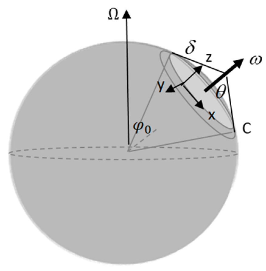
The momentum equation for a material element located on C in the upper layer of two superposed fluids whose density is and depth is [57]:
where is the pressure gradient, the velocity vector ; u and v are the polar and radial current velocities. Since the radius r of C is small compared to the radius R of the earth the Coriolis vector is considered constant around C so that : is the Coriolis vector at the center of the gyre.
Using the polar coordinate and the radial coordinate δ on C, the momentum equations are:
η is the vertical perturbation of the surface height and g the acceleration of gravity. X and Y are the surface stress forcing terms relative to and δ (δ is the distance to the apex of the cone, φ is the polar coordinate).
The equation of continuity on the surface of the cone is:
where E is the evaporation rate. div . In the vicinity of C:
The equation of conservation of the relative vorticity is:
is absolute vorticity.
The relative vorticity ξ ≈ − is the component of the curl of velocity (curl ) perpendicular to the surface of the cone at the considered location.
So in the vicinity of C.
Expanding f versus δ: , the equations of motion A2, A3, A4, A5 along convex paths close to C on the β-cone (, δ) are virtually the same as those expressed on the β-plane (longitude, latitude) . In the first case, the variational calculation is applied to the mean radius of the gyre. In the second case, it is applied to latitude.
The phase velocity is given by the following dispersion relation:
where c is the phase velocity along the equator for the first baroclinic mode and is the latitude of the center of C.
References
- Berger, W. H. (2012). Milankovitch Theory - Hits and Misses. UC San Diego: Scripps Institution of Oceanography. Retrieved from https://escholarship.org/uc/item/95m6h5b9 (accessed on 07 July 2023).
- Raymo, M.E. and Nisancioglu, K.H. (2003). "The 41 kyr world: Milankovitch's other unsolved mystery". Paleoceanography. 18 (1): 1011.
- Lisiecki, L.E.; Raymo, M.E. LR04 Global Pliocene-Pleistocene Benthic d18O Stack; IGBP PAGES/World Data Center for Paleoclimatology Data Contribution Series #2005-008; NOAA/NGDC Paleoclimatology Program: Boulder, CO, USA, 2005.
- Hays JD, Imbrie J, Shackleton NJ (December 1976). Variations in the Earth's Orbit: Pacemaker of the Ice Ages (1976) Science. 194 (4270): 1121–32. [CrossRef]
- Kawamura, K.; Parrenin, F. D. R.; Lisiecki, L.; Uemura, R.; Vimeux, F. O.; Severinghaus, J. P.; Hutterli, M. A.; Nakazawa, T.; Aoki, S.; Jouzel, J.; Raymo, M. E.; Matsumoto, K.; Nakata, H.; Motoyama, H.; Fujita, S.; Goto-Azuma, K.; Fujii, Y.; Watanabe, O. "Northern Hemisphere forcing of climatic cycles in Antarctica over the past 360,000 years". (2007) Nature. 448 (7156): 912–916. [CrossRef]
- Westerhold, T., Marwan, N., Drury, A.J., Liebrand, D., Agnini, C., Anagnostou, E., Barnet, J.S.K., Bohaty, S.M., De Vleeschouwer, D., Florindo, F., Frederichs, T., Hodell, D.A., Holbourn, A.E., Kroon, D., Lauretano, V., Littler, K., Lourens, L.J., Lyle, M., Pälike, H., Röhl, U., Tian, J., Wilkens, R.H., Wilson, P.A., Zachos, J.C., 2020. An astronomically dated record of Earth’s climate and its predictability over the last 66 million years. Science 369, 1383–1387. [CrossRef]
- Berger, A.; Loutre, M.-F. Insolation values for the climate of the last 10 million years. Quat. Sci. Rev. 1991, 10, 297–317.
- Berger, A. Orbital Variations and Insolation Database; IGBP PAGES/World Data Center for Paleoclimatology, Data Contribution Series # 92-007; NOAA/NGDC Paleoclimatology Program: Boulder, CO, USA, 1992.
- Ghil, Michael (1994). "Cryothermodynamics: the chaotic dynamics of paleoclimate". Physica D: Nonlinear Phenomena. 77 (1–3): 130–159. [CrossRef]
- Gildor, Hezi; Tziperman, Eli (2000). "Sea ice as the glacial cycles' climate switch: Role of seasonal and orbital forcing". Paleoceanography. 15 (6): 605–615. [CrossRef]
- Rial, J. A., Oh, J., Reischmann, E., Synchronization of the climate system to eccentricity forcing and the 100,000-year problem. Nature Geoscience, 2013, 6 (4): 289–293. S2CID140578902. [CrossRef]
- Abe-Ouchi, A., et al., Insolation-driven 100,000-year glacial cycles and hysteresis of ice-sheet volume. Nature, 2013, 500 (7461): 190–193. PMID 23925242. S2CID 4408240. [CrossRef]
- Bintanja R., R. S. W. van de Wal, North American ice-sheet dynamics and the onset of 100,000-year glacial cycles. Nature 454, 869–872 (2008).
- Clark P. U., D. Pollard, Origin of the Middle Pleistocene Transition by ice sheet erosion of regolith. Paleoceanography 13, 1–9 (1998).
- Oerlemans, J. (1980). Model experiments on the 100,000-yr glacial cycle. Nature, 287, 430–432.
- Pollard, D. (1983). A coupled Climate-Ice Sheet model applied to the Quaternary Ice Ages. Journal of Geophysical Research, 88, 7705–7718.
- Raymo, M. E. (1997). The timing of major climate terminations. Paleoceanography, 12, 577–585.
- Berends C. J., Köhler P., Lourens L. J., W. van de Wal R. S., On the Cause of the Mid-Pleistocene Transition, 2021, Reviews of Geophysics, 59, 2. [CrossRef]
- Köhler, P., & van de Wal, R. S. W. (2020). Interglacials of the Quaternary defined by northern hemispheric land ice distribution outside of Greenland. Nature Communications, 11, 5124.
- Berends, C. J., de Boer, B., & van de Wal, R. S. W. (2018). Application of HadCM3@Bristolv1.0 simulations of paleoclimate as forcing for an ice-sheet model, ANICE2.1: Set-up and benchmark experiments. Geoscientific Model Development, 11, 4657–4675. [CrossRef]
- Weertman, J. (1961). Stability of Ice-Age Ice Sheets. Journal of Geophysical Research, 66, 3783–3792. [CrossRef]
- Ou H-W, A Theory of Orbital-Forced Glacial Cycles: Resolving Pleistocene Puzzles, J. Mar. Sci. Eng. 2023, 11, 564. [CrossRef]
- Chalk, T.B.; Hain, M.P.; Foster, G.L.; Rohling, E.J.; Sexton, P.F.; Badger, M.P.S.; Cherry, S.G.; Hasenfratz, A.P.; Haug, G.H.; Jaccard, S.L.; et al. Causes of ice age intensification across the Mid-Pleistocene Transition. Proc. Natl. Acad. Sci. USA 2017, 114, 13114–13119.
- Quinn, C.; Sieber, J.; Von Der Heydt, A.S.; Lenton, T.M. The Mid-Pleistocene Transition induced by delayed feedback and bistability. Dyn. Stat. Clim. Syst. 2018, 3, 1–17.
- Clark, P.U.; Archer, D.W.; Pollard, D.; Blum, J.D.; Rial, J.A.; Brovkin, V.; Mix, A.C.; Pisias, N.G.; Roy, M. The middle Pleistocene transition: Characteristics, mechanisms, and implications for long-term changes in atmospheric pCO2. Quat. Sci. Rev. 2006, 25, 3150–3184.
- Hönisch, B.; Hemming, N.G.; Archer, D.; Siddall, M.; McManus, J.F. Atmospheric Carbon Dioxide Concentration across the Mid-Pleistocene Transition. Science 2009, 324, 1551–1554.
- Herbert T. 2023. The Mid-Pleistocene climate transition. Annual Review of Earth and Planetary Sciences. V. 51, pp. 389–418.
- Ganopolski, A.: Toward generalized Milankovitch theory (GMT), Clim. Past, 2024, 20, 151–185. [CrossRef]
- Willeit, M.; Ganopolski, A.; Calov, R.; Brovkin, V. Mid-Pleistocene transition in glacial cycles explained by declining CO2 and regolith removal. Sci. Adv. 2019, 5. [CrossRef]
- Tziperman E., H. Gildor, On the mid-Pleistocene transition to 100-ka glacial cycles and the asymmetry between glaciation and deglaciation times. Paleoceanography 18, 1-1–1-8 (2003).
- Ganopolski A., R. Calov, The role of orbital forcing, carbon dioxide and regolith in 100 ka glacial cycles. Clim. Past 7, 1415–1425 (2011). Climate of the Past, 2011.
- Tabor C. R., C. J. Poulsen, Simulating the mid-Pleistocene transition through regolith removal. Earth Planet. Sci. Lett. 434, 231–240 (2016).
- Saltzman, Barry; Hansen, Anthony R.; Maasch, Kirk A. (December 1984). "The late Quaternary glaciations as the response of a three-component feedback system to Earth-orbital forcing". Journal of the Atmospheric Sciences. 41 (23): 3380–3389. [CrossRef]
- Maslin, M.A., Brierley, C.M., The role of orbital forcing in the Early Middle Pleistocene Transition, Quaternary International (2015). http://dx.doi.org/10.1016/j.quaint.2015.01.047 (accessed on 07 July 2023). [CrossRef]
- Tzedakis, P., Crucifix, M., Mitsui, T. et al. A simple rule to determine which insolation cycles lead to interglacials. Nature 542, 427–432 (2017). https://doi.org/10.1038/nature21364 (accessed on 07 July 2023). [CrossRef]
- Barker S. et al., Persistent influence of precession on northern ice sheet variability since the early Pleistocene, Science, 2022, 376, 6596, 961-967. [CrossRef]
- Mukhin D., Gavrilov A., Loskutov E., Kurths J, Feigin A., Bayesian Data Analysis for Revealing Causes of the Middle Pleistocene Transition, Scientific Reports, 2019, 9:7328. https://doi.org/10.1038/s41598-019-43867-3 (accessed on 07 July 2023). [CrossRef]
- Nyman K. H. M., Ditlevsen P. D., The middle Pleistocene transition by frequency locking and slow ramping of internal period, Climate Dynamics, 2019, 53:3023–3038. https://doi.org/10.1007/s00382-019-04679-3 (accessed on 07 July 2023). [CrossRef]
- Shackleton, J.D., Follows, M.J., Thomas, P.J. et al. The Mid-Pleistocene Transition: a delayed response to an increasing positive feedback?. Clim Dyn (2022). https://doi.org/10.1007/s00382-022-06544-2 (accessed on 07 July 2023). [CrossRef]
- Kaufmann R. K., Juselius K., Testing competing forms of the Milankovitch hypothesis: A multivariate approach, Paleoceanography, 2016, 31, 2.
- Pinault, J.-L. Resonant Forcing of the Climate System in Subharmonic Modes. J. Mar. Sci. Eng. 2020, 8, 60;. [CrossRef]
- Pinault, J.-L. Modulated Response of Subtropical Gyres: Positive Feedback Loop, Subharmonic Modes, Resonant Solar and Orbital Forcing J. Mar. Sci. Eng. 2018, 6, 107;. [CrossRef]
- Pinault, J.-L. Resonantly Forced Baroclinic Waves in the Oceans: Subharmonic Modes. J. Mar. Sci. Eng. 2018a, 6, 78;. [CrossRef]
- Sasaki, Y. N., Minobe, S., and Schneider, N.: Decadal response of the Kuroshio Extension jet to Rossby waves: Observation and thin-jet theory, J. Phys. Oceanogr., 2013, 43, 442–456. [CrossRef]
- Sasaki, Y. N. and Schneider, N.: Decadal shifts of the Kuroshio Extension jet: Application of thin-jet theory, J. Phys. Oceanogr., 2011, 41, 979–993. [CrossRef]
- Taguchi, B., Xie, S.-P., Schneider, N., Nonaka, M., Sasaki, H., and Sasai, Y.: Decadal variability of the Kuroshio Extension: Observations and an eddy-resolving model hindcast, J. Climate, 2007, 20, 2357–2377. [CrossRef]
- Tiéfolo Diabaté S., Swingedouw D., Hirschi J. J-M, Duchez A., Leadbitter P. J., Haigh I. D., and McCarthy G. D., Western boundary circulation and coastal sea-level variability in Northern Hemisphere oceans, Ocean Sci., 17, 1449–1471, 2021. [CrossRef]
- Nilsson, C. S., and G. R. Cresswell, 1980: The formation and evolution of East Australian Current warm-core eddies. Prog. Oceanogr., 9, 133–183. [CrossRef]
- Marchesiello, P., and J. H. Middleton, 2000: Modeling the East Australian Current in the western Tasman Sea. J. Phys. Oceanogr., 30, 2956–2971. [CrossRef]
- Li J., Roughan M. and Kerry C., 2022: Variability and Drivers of Ocean Temperature Extremes in a Warming Western Boundary Current, 2022, Journal of Climate, 35, 1097-1111. [CrossRef]
- Sevellec Florian, Huck Thierry (2015). Theoretical Investigation of the Atlantic Multidecadal Oscillation. Journal Of Physical Oceanography. 45 (9). 2189-2208. https://archimer.ifremer.fr/doc/00281/39189/. [CrossRef]
- Wang, H., Zuo, Z., Zhang, R. et al. Thermodynamic effect dictates influence of the Atlantic Multidecadal Oscillation on Eurasia winter temperature. npj Clim Atmos Sci 7, 151 (2024). [CrossRef]
- Lin, J., & Qian, T. (2022). The Atlantic Multi-Decadal Oscillation. Atmosphere-Ocean, 60(3–4), 307–337. [CrossRef]
- Huang et al, 2017: Extended Reconstructed Sea Surface Temperatures Version 5 (ERSSTv5): Upgrades, Validations, and Intercomparisons. Journal of Climate. [CrossRef]
- NOAA Extended Reconstructed SST V5. A global monthly SST analysis from 1854 to the present derived from ICOADS data with missing data filled in by statistical methods. http://www.esrl.noaa.gov/psd/data/gridded/data.noaa.ersst.v5.html.
- Torrence, C.; Compo, G.P. A practical guide for wavelet analysis. Bull. Am. Meteorol. Soc. 1998, 79, 61–78.
- Gill, A.E. Some simple solutions for heat-induced tropical circulation. Q. J. Royal Met. Soc. 1980, 106, 447–462.
- Pinault, J.-L. A Review of the Role of the Oceanic Rossby Waves in Climate Variability. J. Mar. Sci. Eng. 2022, 10, 493. [CrossRef]
- Pinault, J.-L. Resonantly Forced Baroclinic Waves in the Oceans: A New Approach to Climate Variability. J. Mar. Sci. Eng. 2021, 9, 13. [CrossRef]
- Choi M.Y. and Thouless D.J., Topological interpretation of subharmonic mode locking in coupled oscillators with inertia, Physical Review B, 2001. [CrossRef]
- Lihua Ma, M. Vaquero J.M. 2020. New evidence of the Suess/de Vries cycle existing in historical naked-eye observations of sunspots. Open Astron., V. 29, pp. 28–31.
- Ogurtsov MG, Nagovitsyn YA, Kocharov GE, Jungner H. 2002. Long-period cycles of the Sun’s activity recorded in direct solar data and proxies. Solar Phys, v. 211, pp. 371–394.
- Usoskin, I.G. 2017. A history of solar activity over millennia. Living Rev Sol Phys 14, 3.
- Vaquero J. M., Gallego M. C., García J. A. 2002. A 250-year cycle in naked-eye observations of sunspots. Geophysical Research Letters. V. 29 (20), pp. 58-1-58-4.
- Pinault J-L, Long Wave Resonance in Tropical Oceans and Implications on Climate: The Pacific Ocean, Pure Appl. Geophys., 2015, Springer International Publishing. [CrossRef]
- Pinault J-L, Weakening of the Geostrophic Component of the Gulf Stream: A Positive Feedback Loop on the Melting of the Arctic Ice Sheet, J. Mar. Sci. Eng. 2023, 11, 1689. [CrossRef]
- Pinault J-L, Resonant Forcing by Solar Declination of Rossby Waves at the Tropopause and Implications in Extreme Events, Precipitation, and Heat Waves—Part 1: Theory, Atmosphere 2024, 15, 608. [CrossRef]
- Pinault J-L, Resonant Forcing by Solar Declination of Rossby Waves at the Tropopause and Implications in Extreme Precipitation Events and Heat Waves—Part 2: Case Studies, Projections in the Context of Climate Change, Atmosphere 2024, 15, 1226. [CrossRef]
- Pinault, J.-L. Glaciers and Paleorecords Tell Us How Atmospheric Circulation Changes and Successive Cooling Periods Occurred in the Fennoscandia during the Holocene, J. Mar. Sci. Eng. 2021a, 9, 832. [CrossRef]
- Pinault, J.-L. and Pereira, L., What Speleothems Tell Us about Long-Term Rainfall Oscillation throughout the Holocene on a Planetary Scale, J. Mar. Sci. Eng. 2021, 9, 853. [CrossRef]
- Puetz, A. Prokoph, G. Borchardt, E. Mason, Evidence of synchronous, decadal to billion-year cycles in geological, genetic, and astronomical events Chaos Solitons Fractals, 62–63 (2014), pp. 55-75, doi.org/10.1016/j.chaos.2014.04.001.
- Puetz S. J., Prokoph A., Borchardt G., Journal of Statistical Planning and Inference, 170, 2016, 158-165, doi.org/10.1016/j.jspi.2015.10.006.
- Prokoph A., Puetz S.J., Period-tripling and fractal features in multi-billion-year geological records, Math. Geosci., 47 (5) (2015), pp. 501-520, doi.org/10.1007/s11004-015-9593-y.
- Huggett, Richard J. (2006). The natural history of the Earth: debating long-term change in the geosphere and biosphere. London: Routledge. ISBN 0-203-00407-8.
- Zeebe, R.E.; Lourens, L. Solar System chaos and the Paleocene–Eocene boundary age constrained by geology and astronomy. Science 2019, 365, 926–929.
Figure 1.
Fourier transform of solar irradiance (SI), average of values calculated at 15°N and 65°N in the northern hemisphere from [7,8] representative of the radiative forcing exerted on the North Atlantic gyre. The peak at 23.4 ka reflects precession variations, the one at 41.1 ka reflects obliquity variations, the peaks at higher periods reflect variations in eccentricity. The blue arrows indicate the periods involved in the Mid-Pleistocene Transition (MPT) and the Early Quaternary Transition (EQT). The red arrows indicate the periods which require a latitudinal shift in the centroid of the GRW to resonate. Values in parentheses indicate that the peaks concerned are not directly involved in the transitions.
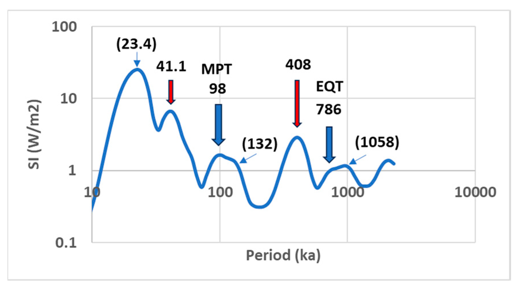
Figure 2.
Coherence and phase of the Sea Surface Temperature (SST) time-averaged over the period of time 1854-2023 (Fourier spectrum), scale-averaged over the period ranges 3-6 years (a, b), 6-12 years (c, d), 12-24 years (e, f), 24-48 years (g, h), and 48-96 years (i, j). The phase is only shown for high values of coherence to improve the readability. Amplitude of the Sea Surface Temperature (SST), time-averaged over 1854-2023, scale-averaged over the period range 6-12 years (k), and amplitude of the zonal geostrophic current time-averaged over 1993-2022, scale-averaged over the period range 6-12 years (l). References are the SST at 46°N, 56°W in (a-k) (the coherence is 1 and the phase 0 at this place) and the zonal geostrophic current at 38.5°N, 62.5°W (l).
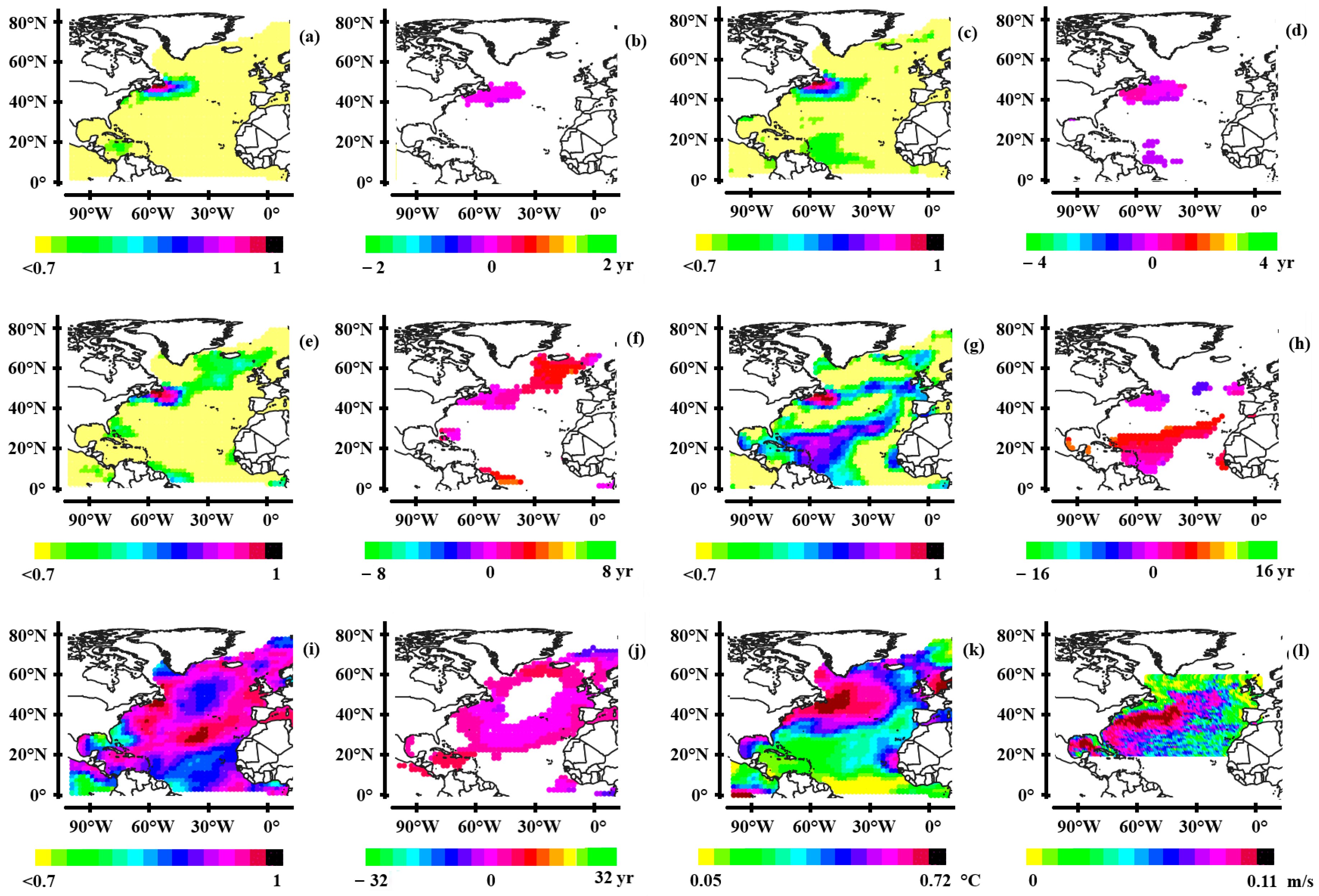
Figure 3.
With the indicated transformation, the equations of motion of Rossby waves remain virtually unchanged (Appendix A), except that the waves wind around themselves around the gyre, which give them special properties. This is why they are called Gyral Rossby Waves (GRWs). In blue is represented what concerns the equations of motion, in pink what concerns their solutions.
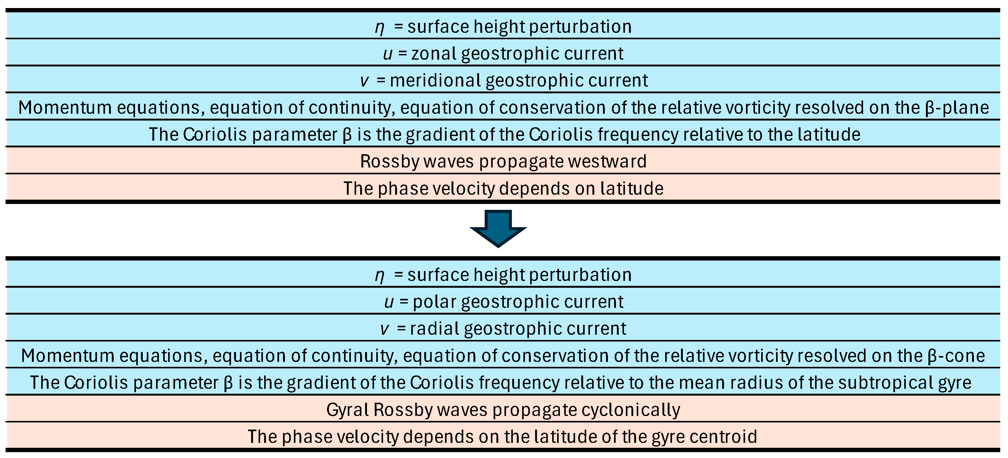
Figure 4.
Exchange zones of subharmonic couples of average periods (1 yr-4 yr) in (a), (4 yr-16 yr) in (b), (4 yr, 64 yr) in (c), and (32 yr, 64 yr) in (d). These zones which cause resonant forcing to occur in subharmonic modes, according to the system of Caldirola-Kanai (CK) equations (1), are defined from the joint coherence of the coupled waves: the areas in red are such that the mean coherence of the coupled waves is higher than 0.85.
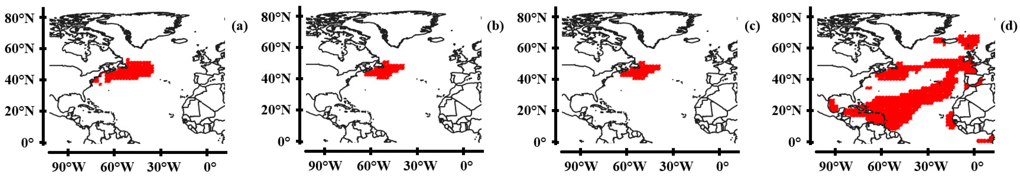
Figure 5.
- Shifting of the period of eccentricity in the vicinity of 100 ka from [7]– (a) Fourier transform of solar irradiance over successive time segments – (b) Maxima of the Fourier transforms versus time (middle of the successive time segments). The period of resonance (98.3 ka) is represented by an orange dotted line.
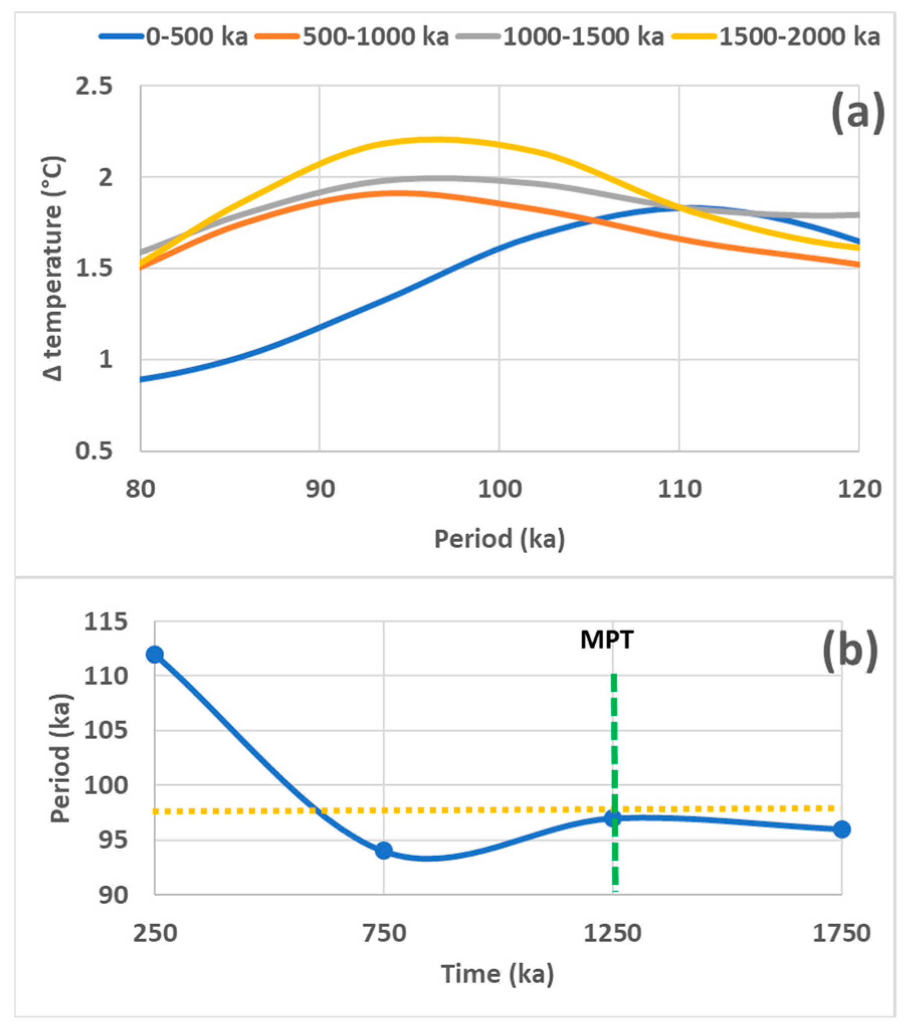
Figure 6.
Orbital forcing and de-trended global temperature response into the shifted period range 28.8 - 65.5 ka representative of the 41-ka period of obliquity, and the period range 73.7 – 147.5 ka representative of the 98-ka period of eccentricity (Figure 1, Table 1) —(a) Comparison of the observed and modeled global temperature variations within the shifted period range 28.8 - 65.5 ka – (b) Comparison of the observed and modeled global temperature variations within the period range 73.7 – 147.5 ka – (c) Climate sensitivity within 28.8 - 65.5 ka and 73.7 – 147.5 ka period ranges. The shifted period range corresponding to the subharmonic mode is deduced from Table 1 by considering that the period to be framed is no longer 49.2 ka, but 41 ka. The dotted green line indicates when the transition occurs (≈1250 ka ago).
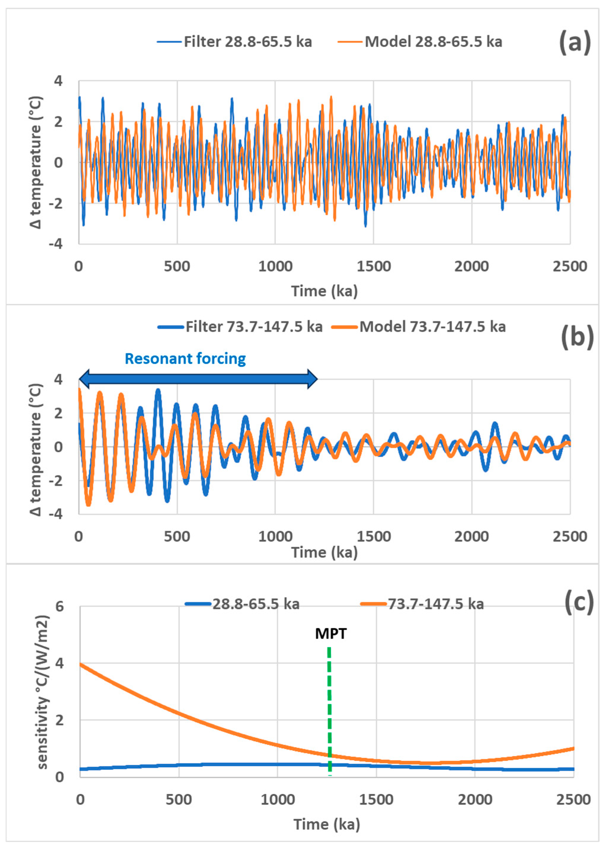
Figure 7.
Shifting of the period of eccentricity in the vicinity of 800 ka from [7]– (a) Fourier transform of solar irradiance over successive time segments – (b) Maxima of the Fourier transforms versus time (middle of the successive time segments). The period of resonance (786.4 ka) is represented by an orange dotted line.
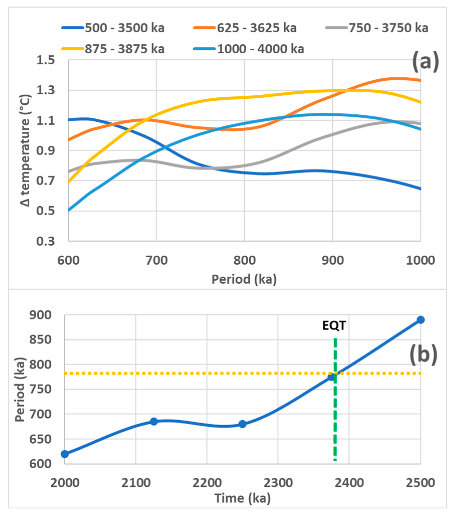
Figure 8.
Orbital forcing and de-trended global temperature response into the period range 295 - 590 ka representative of the 408-ka period of eccentricity, and the period range 590 – 1180 ka representative of the 786-ka period of eccentricity (Figure 1, Table 1) —(a) Comparison of the observed and modeled global temperature variations within the period range 295 - 590 ka – (b) Comparison of the observed and modeled global temperature variations within the period range 590 – 1180 ka – (c) Climate sensitivity within 295 - 590 ka and 590 – 1180 ka period ranges. The dotted green line indicates when the transition occurs (≈2380 ka ago).
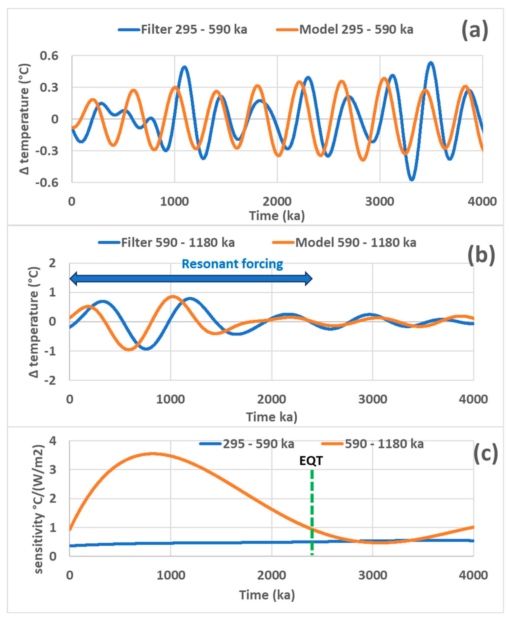
Figure 9.
Deviation between the phases of orbital forcing calculated by Berger et Loutre [7] and Zeebe et Lourens [75]. The two period ranges considered are representative of the 408-ka and 786-ka periods of eccentricity.
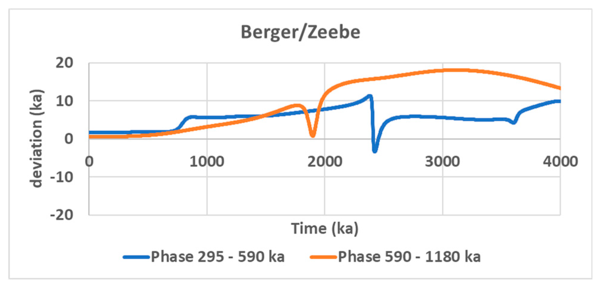
Figure 10.
Comparison of the observed and modeled global temperature variations within the period range 73.7 – 147.5 ka.
Figure 10.
Comparison of the observed and modeled global temperature variations within the period range 73.7 – 147.5 ka.
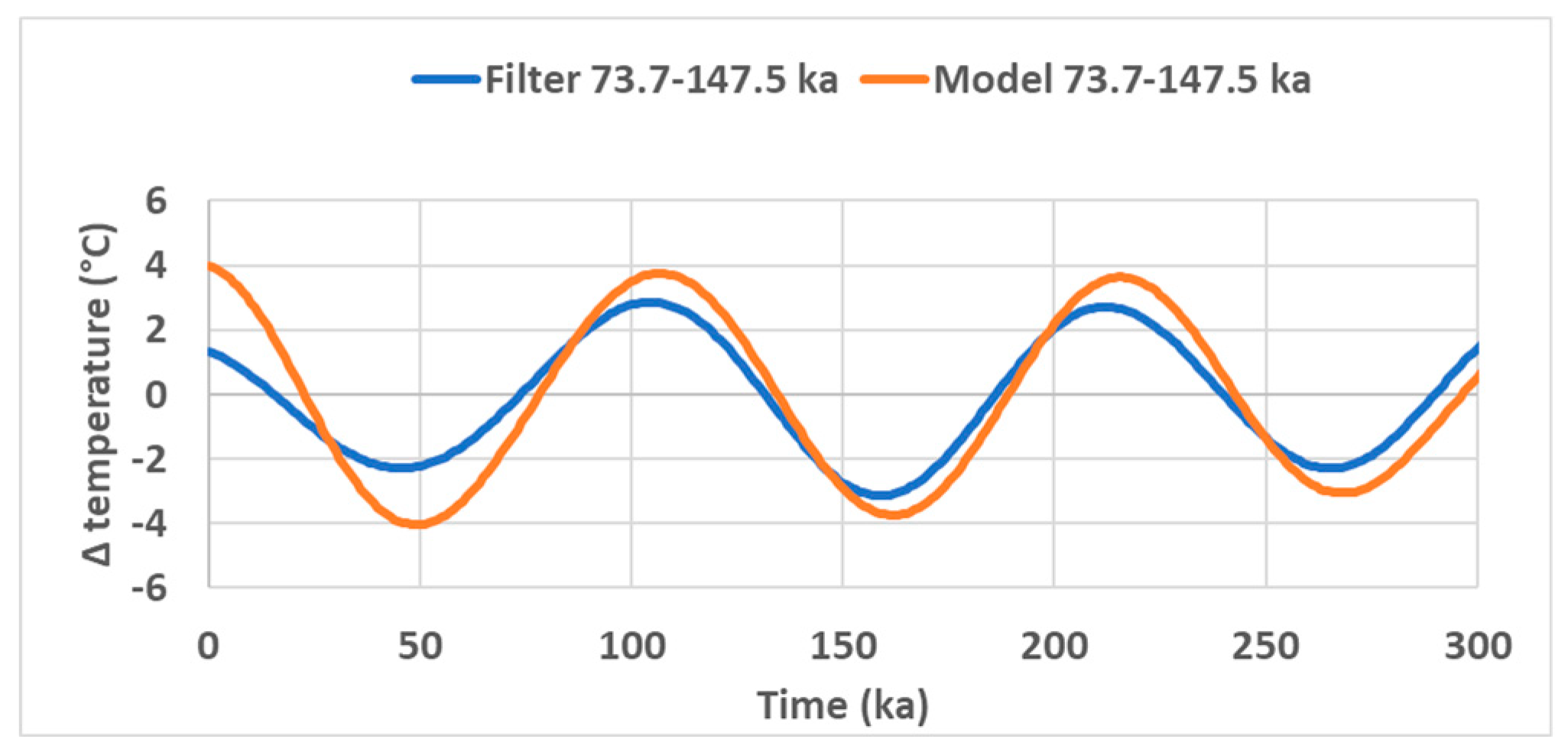
Figure 11.
Last glacial – interglacial and western boundary current acceleration phases in the period range 73.7 – 147.5 ka. The red arrow indicates the end of the expansion of sea ice (southernmost limit of sea ice nearly 21 ka BP).
Figure 11.
Last glacial – interglacial and western boundary current acceleration phases in the period range 73.7 – 147.5 ka. The red arrow indicates the end of the expansion of sea ice (southernmost limit of sea ice nearly 21 ka BP).
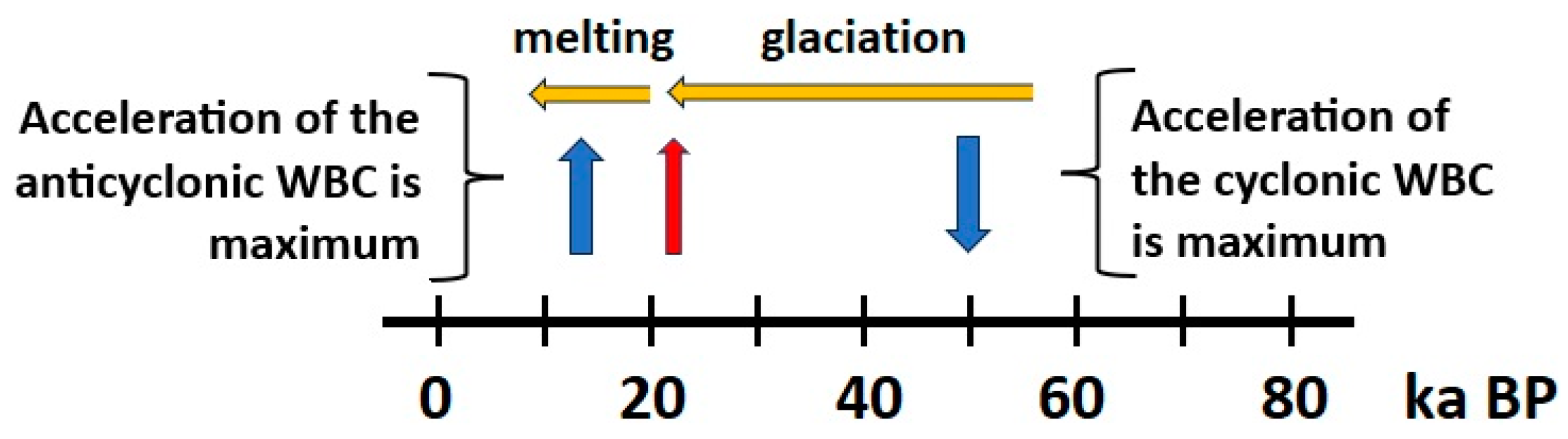
Figure 12.
Acceleration vectors of the geostrophic polar current, and sea ice edge motion – (a) 50 ka ago – (b) 12 ka ago. The current winter ice edge and 21 ka ago (southernmost limit during the last glaciation) are represented by thin blue lines. The acceleration of the polar geostrophic current of the North Atlantic gyre is represented by brown arrows. The wide blue arrows indicate the motion of the edge of sea ice in winter.
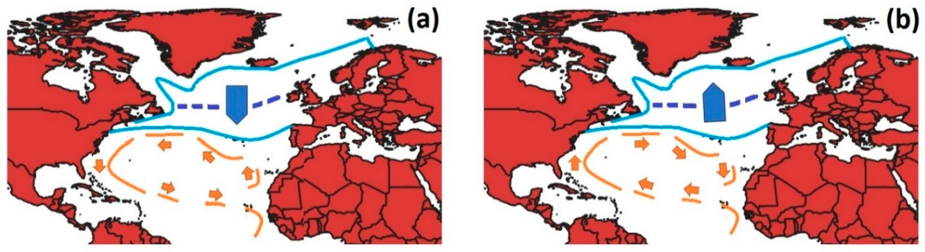

Table 1.
The natural periods of Gyral Rossby Waves (GRWs) and the period ranges of subharmonic modes in the North Atlantic. From [41], Table 1, with kind permission from Journal of Marine Science and Engineer (JMSE).
| Rank | Band Width (yr) | Natural Periods of GRWs (yr) | Subharmonic Mode | Forcing Mode |
| 1 | 48 - 96 | 64 | Solar forcing (Gleissberg cycle) | |
| 2 | 96 - 192 | 128 | Solar forcing (Gleissberg cycle) | |
| 3 | 192 - 576 | 256 | Solar forcing (de Vries/Suess cycle) | |
| 4 | 576 - 1152 | 768 | No external forcing | |
| 5 | 1152 - 2304 | 1536 | Solar forcing (Hallstatt cycle) | |
| 6 | 2304 - 4608 | 3072 | No external forcing | |
| 7 | 4608 - 9216 | 6144 | No external forcing | |
| 8 | 9216 – 18,432 | 12,288 | No external forcing | |
| 9 | 18,432 – 36,864 | 24,576 | Orbital forcing (precession) | |
| 10 | 36,864 – 73,728 | 49,152 | Orbital forcing (obliquity) | |
| 11 | 73,728 – 147,456 | 98,304 | Orbital forcing (eccentricity) | |
| 12 | 147,456 - 294,912 | 196,608 | No external forcing | |
| 13 | 294,912 - 589,824 | 393,216 | Orbital forcing (eccentricity) | |
| 14 | 589,824 - 1,179,648 | 786,432 | Orbital forcing (eccentricity) | |
| 15 | 1,179,648 – 2,359,296 | 1,572,864 | No external forcing |
Disclaimer/Publisher’s Note: The statements, opinions and data contained in all publications are solely those of the individual author(s) and contributor(s) and not of MDPI and/or the editor(s). MDPI and/or the editor(s) disclaim responsibility for any injury to people or property resulting from any ideas, methods, instructions or products referred to in the content. |
© 2025 by the authors. Licensee MDPI, Basel, Switzerland. This article is an open access article distributed under the terms and conditions of the Creative Commons Attribution (CC BY) license (http://creativecommons.org/licenses/by/4.0/).
Copyright: This open access article is published under a Creative Commons CC BY 4.0 license, which permit the free download, distribution, and reuse, provided that the author and preprint are cited in any reuse.


