
Submitted:
26 November 2025
Posted:
02 December 2025
You are already at the latest version
Abstract
This study presents the development of a smart microgrid control framework. The goal is to achieve optimal energy management and maximize photovoltaic (PV) generation utilization through a combination of optimization and reinforcement learning techniques. A detailed Simulink model is developed in MATLAB to represent the dynamic behavior of the microgrid, including load variability, temperature profiles, and solar radiation.
Initially, a genetic algorithm (GA) is used to perform static optimization and parameter tuning – identifying optimal battery charging/discharging schedules and balancing power flow between buildings in the microgrid to minimize main grid dependency. After that a Soft Actor-Critic (SAC) reinforcement learning agent is trained to perform real-time maximum power point tracking (MPPT) for the PV system under different environmental (weather) and load conditions. The SAC agent learns from multiple (eight) simulated PV generation scenarios and demand profiles, optimizing the duty cycle of the DC-DC converter to adaptively maintain maximum energy yield. The combined GA-SAC approach is validated on a university campus microgrid consisting of four interconnected buildings with heterogeneous loads, including computer labs that generate both active and reactive power demands. The results show improved efficiency, reduced power losses, and improved energy autonomy of the microgrid, illustrating the potential of AI-driven control strategies for sustainable smart energy systems.
Keywords:
intelligent control framework
; optimization
; microgrid energy management
1. Introduction
The In recent years, the global energy sector has been undergoing a fundamental transformation, with the massive deployment of renewable energy sources (solar, wind), the growing role of battery energy systems, and the increasing importance of decentralized energy production and storage. In this context, microgrid systems are becoming a leading platform for integrating distributed energy resources, managing loads, and optimizing the interaction with the central grid. They offer the possibility of higher energy autonomy, better flexibility, and lower operating and investment costs, as well as improved stability and quality of power supply. However, the effective management of microgrid systems hides many technological challenges: the instability and unpredictability of renewable energy generation, the need to balance active and reactive power, the limited ability of batteries to cover sudden changes, and the need to minimize the exchange with the public grid. These aspects make optimal microgrid control a complex task, which is often formulated as a minimization of multiple objectives — costs, emissions, system wear, power quality, etc. (see e.g. review articles [1,2,3]).
The present study aims to develop and implement a comparative approach for microgrid control, which combines two modern methodologies: static optimization using a genetic algorithm (GA) [4] and online adaptive control using an agent with reinforcement learning (RL) [5]. The selected microgrid environment includes photovoltaic generators, a battery and grid exchange, with the focus on optimizing the MPPT (maximum power point tracking) mode and balancing P–Q components. This environment corresponds to a real university campus microgrid consisting of four interconnected buildings (UBT) in Pristina, Kosovo The organization of the study is as follows: first — generation of scenarios for the PV potential and load, second — GA optimization of a daily plan for battery charging/discharging and minimizing the grid power, third — training a SAC (Soft Actor–Critic) agent offline on the same scenarios, fourth — comparative analysis of the results through metrics such as RMSE (Root Mean Square Error) for State of Charge (SOC) and power balance Pgrid, as well as time graphs for key scenarios, and fifth — upgrading the reward function of the RL agent for improved precision and approximation to GA solutions. Such a structural approach allows not only to evaluate how the RL agent can approach or surpass static optimization, but also to investigate how different scenarios of energy generation (e.g. “clear day”, “intermittent clouds”, “low yield”) and load affect the behavior of the system. By applying this methodological process, the aim is to achieve a controller that is not only optimal for a given scenario, but also sufficiently adaptive to changes in conditions — important for real-world microgrid applications with dynamic behavior.
Furthermore, the performed comparative analysis through specific metrics and visualizations will create a baseline for further research — for example, the inclusion of tariffs, battery degradation, real-time control or hybrid GA-RL strategies. As a result, the present work has the potential to contribute to the practical implementation of smart microgrid controllers with high efficiency and resilience, as well as to enrich the literature with comparative results between GA and RL approaches.
2. Related Works
In the paper [6] the aim is to present an overview of optimization strategies for Energy Management Systems (EMS) in microgrids: to classify, compare, deduce trends and research gaps. The authors point out that although research in this area is increasing, there are several key gaps: less real experimental data, need for investigation of “real-time” systems, integration of machine learning with optimization approaches, better handling of uncertainty.
The work [7] presents a comprehensive review of the use of artificial intelligence (AI) techniques—including machine learning, neural networks, and reinforcement learning—in microgrid control. The article maps the current state of research, describes control system architectures, identifies key challenges, and outlines future directions for development in the field. The authors analyze several existing control architectures for microgrids (e.g., hierarchical control layers — primary, secondary, tertiary control) and note their limitations in the case of high dynamics, unstable RES generation and uncertainty. They present a classification of AI techniques used in microgrids — forecasting, optimization, control, fault detection — and discuss their applications and limitations. The conclusions are that AI-based systems show promising potential for improving the flexibility, energy efficiency, and self-management of microgrids. However, the authors identify a number of emerging challenges: the need for sufficient training data, interpretability and trust in AI controllers, compatibility with real power systems, cybersecurity, and security.
The paper [8] provides a comprehensive overview of microgrid control strategies and proposes an integration with model-free reinforcement learning (MFRL). The authors develop a “high-level” research map of microgrid control from six different perspectives (operation mode, function, time scale, hierarchy, communication, control techniques). They then consider modular building blocks for two main types of inverters—grid-following (GFL) and grid-forming (GFM)—and how RL can “fit” into existing control architectures. They present three ways to fuse MFRL with traditional control:
• model identification and parameter tuning,
• supplementary signal generation from RL,
• controller substitution with RL policy.
Finally, key challenges are discussed – e.g., stability, safety, communication, learnability, interpretability – and a vision for the future of RL in microgrid control is provided.
The paper [9] investigates applying the Perturb and Observe (P&O) algorithm, which is often compared to intelligent MPPT algorithms, including RL-based approaches (such as SAC). The authors develop an artificial intelligence (AI)-based energy management system (EMS) in a direct current (DC) microgrid. The system uses a combination of:
• multiple renewable sources (Photovoltaic (PV) panels and wind turbines (WT)),
• a Li-ion battery as a storage system,
• and a backup grid for cases of insufficient power generation.
The control includes:
• the use of MPPT (Maximum Power Point Tracking) for PV and WT,
• a multi-agent system (MAS) for coordination between individual sources and system elements,
• artificial neural network controllers (ANNC) for battery charging/discharging and DC bus stabilization.
The goal is to maintain power balance in the microgrid and a stable operating state under variable conditions — in real time. The architecture is decentralized, MAS-based: separate agents for PV MPPT, wind MPPT, battery, loads and backup grid are included. The system uses JADE (Java Agent Development Framework) for the agents and MACSimJX for the interface between MATLAB/Simulink and the agents. Simulations show that the proposed EMS architecture is flexible and able to keep the DC-line stable under changes in generation and load.
The authors of [10] propose a neural network-based energy management system (EMS) (NN-EMS) for islanded AC microgrids that operate with multiple PV-battery-based distributed generators (DG).
Key problem addressed: non-uniform insolation leads to different generated power from PV systems, which causes non-uniform state of charge (SOC) among the batteries. Over time, this can lead to some batteries reaching SOC limits and unable to support the DC-link of the system.
The NN-EMS system is trained to “learn” an optimal state-action according to the results of the optimal power flow (OPF) of the system. In this way, the model can respond in near real-time to changes in PV power without having to solve the OPF daily.
A training dataset is generated by solving a Mixed-Integer Linear Programming (MILP) OPF problem for an islanded microgrid with droop control, under practical generation and load profiles. A neural network is then trained that accepts inputs such as current generation, consumption, battery SOC and outputs a control solution (e.g., battery power) to balance the SOCs and maintain the system. The controller is validated in a CIGRE LV microgrid testbed with PV-battery DGs. It is noted that this NN-EMS controller does not require an accurate generation or load forecast, which is an advantage over classical prediction and optimization methods.
The system responds quickly to changes in PV power — by directly applying a neural policy without the need for repeated OPF solutions. Advantage: greater operational flexibility and reduced generation/load forecasting requirements.
The work [11] presents a new framework for coordinated operation of a microgrid with a hybrid energy storage system (HESS) including a battery (high energy density) and a supercapacitor (high power density). The system is controlled in two time-scales:
1. First phase (longer scale, e.g., hours): A plan for battery operation and grid exchange is decided based on predicted generation and load data, without taking into account unpredictable deviations. This phase is formulated as a nonlinear optimization. SpringerOpen+1
2. Second phase (real-time, shorter scale, e.g., minutes): After the real generation with unpredictable fluctuations is realized, corrective actions are applied by a deep reinforcement learning agent — specifically, the Soft Actor Critic (SAC) algorithm. Here, the task is to compensate for deviations from the plan and maintain the balance between generation, load, battery, and grid. SpringerOpen+1
This achieves multi-timescale coordination: the battery covers the long-term energy balance, the supercapacitor responds to sudden fluctuations, and the RL agent provides real-time adaptation.
Additionally, the authors include battery and supercapacitor degradation models, which allows for simultaneous optimization of operating and investment costs.
Through simulations in MATLAB, with a horizon of 48 h and time steps of 1 h (phase 1) and 5 min (phase 2), the authors show that the approach improves stability and reduces variations in the exchange with the network. The RL agent (SAC) is trained quite quickly — multiple episodes lead to convergence of the reward. The combined scheme shows that when using a battery + supercapacitor + RL controller, lower operating costs and more flexible response to fluctuations are achieved than with traditional strategies.
The authors of [12] propose a model-free approach to maintain stable voltage in microgrid systems with high resistance/reactive ratio (R/X), where active power strongly influences voltage — a situation typical for distribution networks and microgrids.
A significant contribution is the use of the Soft Actor–Critic (SAC) algorithm for battery energy system (BESS) control to provide “voltage support” — i.e., reducing voltage deviations by dynamically controlling active and reactive power from the energy storage system. This achieves greater stability and power quality in a microgrid, especially when traditional reactive strategies (Q-control) are insufficient for a high R/X microgrid.
Simulations in MATLAB/Simulink environment using a test system in Cordova, Alaska, show that the implementation of SAC-based control achieves a significant reduction in voltage deviations — approximately 2.5 to 4.5 times less compared to standard methods. Control through ESS (energy storage systems) allows both active power (P) and reactive power (Q) to participate in voltage maintenance, which is key for high R/X microgrids, where active power has a significant effect on voltage. Based on RL, the approach does not require a detailed physical model of the system (“model-free”), which facilitates its applicability to real systems with unknown or variable characteristics.
The study [13] addresses real-time planning and control of microgrids under high uncertainty conditions (RES generation, load, storage), where traditional control algorithms (propertybased or MPC) face the need for a rich model and large amounts of data.
The authors propose a hybrid approach that combines a reinforcement learning (RL) algorithm with meta-learning, specifically the Model Agnostic Meta Learning (MAML) method integrated with Soft Actor–Critic (SAC) — denoted as MAML-SAC. This allows the model to adapt quickly to a new microgrid environment with little data, by pre-training a baseline policy and then fine-tuning it.
In the “early phase” of microgrid operation (when data is scarce), MAML-SAC achieves significantly better results than traditional SAC — lower operating costs, faster adaptation to different tasks. For diverse and variable scenarios, the meta-RL approach shows advantages.
The study [14] presents a new distributed control for DC microgrid systems, focused on minimizing the generation cost by implementing a Soft Actor–Critic (SAC) algorithm. The system is architecturally distributed — each generator/subsystem in the microgrid acts as an agent that makes local decisions, but with a global goal: overall minimizing the cost of energy generation and maintaining the voltage/current in an optimal mode.
A SAC approach is used for each subsystem, with the exchange of certain signals between the agents (coordination), which makes the control decentralized but coordinated. This is significant because in real DC microgrids the control is often distributed (many devices), and the centralized approach may suffer from scalability and communication limitations.
In simulations, the authors show that their SAC-based approach achieves lower costs than traditional optimal control methods (e.g., centralized algorithms) under dynamic load and energy generation conditions. Additionally, the approach exhibits good adaptability and a distributed architecture, which reduces communication overhead and increases fault tolerance. This methodology confirms that SAC can be applied not only for battery management, but also for energy generation optimization and economic purposes.
The authors of [15] propose an innovative approach for resilient energy trading in a system of interconnected microgrids, using a Soft Actor–Critic (SAC)-like algorithm in combination with a Long Short Term Memory (LSTM)—i.e., LSTM-SAC. The main goal is to cope with high load uncertainty and distributed generation, as well as extreme events such as generator failures and grid outages.
In simulations on a microgrid system based on IEEE 14 bus topology, the LSTM-SAC approach shows that it can support efficient energy trading and resilience against extreme conditions. In the presence of failures (e.g., generator failure, line outage), the agent manages to maintain a higher level of trading, lower losses, and more stable operation compared to baseline solutions without RL and without LSTM component. As a result, training with LSTM-SAC contributes to better tracking of historical trends and adaptation in changing environments, improving the resilience of the microgrid network.
A data-driven Adaptive Load Frequency Control (ALFC) for islanded microgrids that combines the objectives of frequency stability and economic efficiency is proposed in [16]. The key innovation is the {Priority Replay - Soft Actor–Critic (PR-SAC)} algorithm, which uses:
• entropy regularization to make the policy more diverse and adaptive
• prioritized experience replays for faster and more efficient learning.
Through this multiobjective approach, the agent can balance several metrics when managing a microgrid environment with high unpredictability.
In simulations (e.g., 24-hour horizon with random fluctuations), PR-SAC demonstrates better performance — on average, lower frequency deviation and lower generation costs — compared to baseline algorithms such as PPO, DDPG, and others. For example, the authors note that the frequency deviation for PR-SAC is between 1.09 and 3.20 times lower than that of other algorithms. The algorithm also shows good adaptability to different types of disturbances (step, square, noise) and robust performance under random conditions.
The aim of the study [17] is to propose a framework for joint optimization of a multi-microgrid system with a shared energy storage system (ESS). The study uses a multi-agent stochastic game model and reinforcement learning algorithms to coordinate actions between different microgrids so that the overall use of the ESS is optimized — minimizing costs, improving reliability, reducing peaks, and maximizing the use of renewable energy.
In simulations, the system with several microgrids + shared ESS shows lower operating costs and better utilization of renewable energy compared to autonomous control (“each microgrid on its own”). The multi-agent reinforcement learning (MARL) approach outperforms the centralized approach in cases of high volatility of renewable generation and shared load, as agents adapt and coordinate dynamically. The authors show that shared ESS leads to synergy — when one microgrid has a surplus of energy, it can charge an ESS, which then serves another microgrid in deficit, coordinated through the agents.
The authors of [18] consider a multi-microgrid (MMG) scenario, where each microgrid has renewable generation and can trade/share energy with the others. The goal is to ensure joint optimization of the operation of all microgrids — through coordination, shared trading, and optimal use of resources.
Simulations show that the proposed MASAC approach significantly outperforms other deep reinforcement learning (DRL) algorithms in terms of economic efficiency (lower costs) and computational efficiency (faster learning/better generalization). Microgrids in a cooperative system manage to achieve higher efficiency through trading and sharing of resources, which in the traditional independent mode would be impossible or less efficient. The algorithm shows good adaptability to uncertainties (e.g., variable generation and loads), thanks to AutoML hyperparameterization and the multi-agent approach.
The study [19] proposes a hybrid optimization framework integrating genetic algorithm (GA) optimization, heuristic control, reinforcement learning (RL), and LSTM-based load forecasting for real time energy management in microgrids. Real-world problems are solved to optimize the power imbalance, energy stability, and battery performance. The results show that the adaptive learning-based control and the predictive analytics can provide an intelligent energy management in fluctuating grid conditions.
The studies cited above show that the current trend for intelligent energy management in microgrids is the use of artificial intelligence with reinforcement learning, most often applying a single-agent or multi-agent approach. In this case, very often, SAC agents are used, which are suitable for training and implement successful policies in real critical situations. These results give rise to the application of a similar approach in the present study on energy management in a real microgrid.
In literature and practice, two main modes of PV operation are often discussed [20]:
• MPPT (Maximum Power Point Tracking) - the goal is to extract the maximum available power from the PV module under given lighting and temperature conditions. This is the classic "maximum power point" mode because the system strives for the maximum power point on the P-V curve.
• Curtailment / Power Limiting Mode - sometimes it is not necessary the PV to give its full maximum (for example, if the battery is fully charged or if the tertiary level has set a limit due to network conditions or economic reasons). Then the controller limits the output below the maximum.
The authors of [21] consider a system with a photovoltaic panel, a DC–DC boost converter and a grid-connected PV system and aim to improve the maximum power point tracking (MPPT) strategy by optimizing controllers with a genetic algorithm (GA).
The main goal is to compare the strategies:
• Perturb and observe (P&O) method + PI controller,
• Fuzzy Logic + PI controller, whose parameters are optimized by a genetic algorithm.
The genetically optimized Fuzzy-PI structure gives the best compromise performance among the considered options.
In our study, the goal is to extract maximum power from the PV module given the available solar irradiation and environment temperature. Since this process requires real-time adjusting duty cycles and control parameters, applying the actor-critic approach is very suitable. For this reason a SAC agent is trained to perform real-time MPPT for the PV system.
3. The Microgrid Setup
The microgrid, considered in the current study is the real microgrid – university campus of the UBT – college in Pristina, Kosovo (https://www.ubt-uni.net/en/home/). The microgrid is main grid connected and operates a PV system, as well as a Battery energy storage (BES) system.
The studied microgrid is composed by the following components:
- Buildings. The microgrid includes 4 buildings. Photovoltaic panels are installed on the roofs of the buildings. Statistical data on the electricity produced by the PV system, as well as the energy consumption of the university campus were used.
- PV system. The photovoltaic panels used are from type CHSM72M-HC 450, made of polycrystalline silicon (see [22]). The area of the panels in the PV system is 840,2 m2. The peak power production of the PV system (in a summer day) is 204 kW. The PV system is connected to the AC electrical system of the microgrid by inverters from type inverters type KAC 50.TL3.
- Battery energy storage system. The maximal capacity of the BES system is 450 kWh. The system has maximal energy exchange capacity (charging/discharging) of 45 kW per hour. AC/DC bidirectional inverters for connection to the AC microgrid system are used. The power consumption of the university campus microgrid is covered by the PV system energy production and the discharging energy from the BES system. The main grid supplies the necessary energy to cover the lack of energy in the microgrid, when it is necessary. In the moments of a surplus energy produced in the microgrid, the excess is accepted by the main grid at a certain price.
- Energy management system. An EMS controls optimally the microgrid energy flows in a real-time. EMS sends signals S1, S2, and S3 correspondingly to the Point of Common Coupling (PCC), the Battery management (BM) of BES system and the MPPT of PV system (see Figure 3 and Figure 4).
The Energy Management System (EMS) sends signals for the optimal management of PV system MPPT mode. It also regulates the charging/discharging schedule of the BES system. The aim is to achieve good power balance in the microgrid and to minimize its energy consumption from the main grid. In Figure 4 is presented the scheme with the input and output signals of the EMS.
SOC denotes the state of charge of the BES system, V_bus_DC is the value of the DC bus voltage, V_b and I_b are the ESS input signals from BES system, and V_PV and I_PV are the input signals from the PV system.
4. Methodology
This section presents the methodology applied in the study.
4.1. General Approach and Goal
This study aims to develop and evaluate an integrated methodology for microgrid optimization and control based on two complementary approaches:
(1) static optimization using a Genetic Algorithm (GA), and
(2) reinforcement learning (RL) using a Soft Actor–Critic (SAC) agent.
The main objective is to minimize the dependence of the microgrid on the main grid by achieving optimal active and reactive power distribution, stable battery state of charge (SOC) management, and maintaining energy balance under the uncertainty of renewable sources.
4.2. Conceptual Framework
The methodology combines three key levels of modeling:
1. Physical-technical level – simulation of a microgrid with a photovoltaic (PV) system, a battery and a load. Each element is modeled using real 24-hour generation and consumption profiles.
2. Optimization level (GA) – static optimization of the power distribution between PV, battery and grid, for a given generation and load scenario.
3. Intelligent control with reinforced learning (RL) – training of a SAC agent, which self-learns offline by interacting with a simulated environment and subsequently controls the microgrid in real time.
Thus, a two-stage methodology is implemented – GA provides the basic optimal strategy, and the RL agent improves the control in dynamic conditions.
Flow-chart of the methodology is presented in Figure 5.
4.3. Modeling the Microgrid Environment
When an electrical system includes heterogeneous (inductive and capacitive) loads, a phase difference occurs between the voltage and current waveforms, creating reactive power. This power is different from the active power associated with performing "useful work". In the cases of university campuses, usually there arise reactive power, due to the use of computers, electrical motors, transformers and other heterogeneous loads.
In the presence of reactive power, the total apparent power of the building is:
where:
• P(t) — active power (real consumption),
• Q(t) — reactive power (influence from computers, Uninterruptible Power Supply (UPS), etc.).
The power factor pf is:
and for a campus with mixed loads often cos(φ)=0.9.
In case that data on the consumed active power in the microgrid Pload(t) is available, the reactive power in the microgrid is calculated as:
Qload(t) = Pload(t)⋅tan(arccos(0.9))
The here considered microgrid is modeled in MATLAB/Simulink environment and includes:
• PV generator with nominal power of 204 kW,
• Battery with capacity of 450 kWh, maximum charge/discharge power ±45 kW and its state of charge (SOC) limits from 20% to 100%,
• Load with 24-hour consumption profile,
• Reactive power Q at cos (φ) = 0.95,
• Connection to the main grid - Point of Common Coupling (PCC), allowing two-way energy exchange.
At the PCC level, complex power is used:
S(t) = P(t) + jQ(t)
The power balance is defined as:
and
where Pbat(t), Qbat(t) are the controlled signals from the agent. In our case Qpv(t) = 0.
Pgrid(t) = Pload(t) – Ppv(t) – Pbat(t)
Qgrid(t) = Qload(t) – Qpv(t) – Qbat(t),
4.4. Static Optimization via Genetic Algorithm (GA)
GA is used to identify the optimal daily battery power profile Pbat(t), t = 1,…, 24; that minimizes the overall grid dependency and losses from inefficient capacity utilization. Let the battery capacity be denoted by Cbat,max.
Decision variables:
x = [Pbat, 1, Pbat, 2, …, Pbat, 24]
Let State Of Charge SOC(t) be the energy in the battery [kWh], and Δt — time interval of one hour [h]. By convention:
- Pbat, t, > 0 : battery discharging,
- Pbat, t, < 0 : battery charging,
- SOCt ∈ [SOCmin, SOCmax].
SOC is updated according to the formula:
where Δt = 1 hour. It is assumed that Pch(t) < 0, and Pdisch(t) > 0. Charging and discharging at the same time is impossible, i. e. when Pch(t) ≠ 0, Pdisch(t) = 0, and vice versa when Pdisch(t) ≠ 0, Pch(t) = 0.
Constraints:
and
Pch(t)Pdisch(t) = 0
SOCmin ≤ SOC(t) ≤ SOCmax
At the end:
SOCmin and SOCmax in equation (10) are fixed at 20% and 100% of Cbat,max respectively.
The constraint (12) ensures the same value of SOC at the end of the 24h period as at the beginning of that period (SOC(0)=SOC(24)). SOC(1) and SOC(24) are fixed at 50% of Cbat,max.
Power factor requirement in PCC (by grid code)
Minimum pfmin ∈ (0,1] ⇒ allowable Qgrid:
or in the case of a hard limit:
|Qgrid(t)| ≤ tan(arccos(pfmin))|Pgrid(t)|
|Qgrid(t)| ≤ Qgrid, max
Linearmodel(LinDistFlow/Thévenin) for the voltage at the Point of Common Coupling (PCC):
Per-unit (pu) approximation [23,24]:
where and are “equivalent” resistances / reactances between PCC and a harder point of the grid (they can be parameters of the environment). Vbase is the nominal voltage in PCC. The formula (15) can be presented in the form:
where
and R′, X′ are sensitivities (dimensionless). 0.95 ≤ ≤ 1.05.
Sbase is the microgrid rating.
This model captures the first order dependence of voltage on power flow, accurate enough for operational optimization and voltage penalties.
Price profile (day/night) and asymmetry purchasing↔selling
• Hourly purchase price Cbuy(t): 0.124 $/kWh for 06:00–21:59 and 0.062 $/kWh for 22:00–05:59 (in the code: night hours 22, 23, 0–6) [25].
• There are no FiT (feed-in tariff) → resale does not bring revenue; in order not to cause “excessive resale”, we impose asymmetric weights:
o heavier penalty for positive P+grid (purchasing energy from the main grid),
o lighter for negative P–grid (resale / selling energy to the main grid).
Objective function to be minimized:
where:
• wP – active power coefficient (usually = 1),
• wQ – reactive power coefficient,
• wSOC – charge stability coefficient for smoothness of SOC (usually = 0.05).
• SOCtarget(t) – desired SOC profile (it could be flat or set according to an energy plan)
• = max() (purchasing)
• = max() (selling)
• is hinge with “deadband”, where V ∈ [Vmin, Vmax]; Dead band is an interval around the nominal value in which the regulator does NOT take action to avoid: unnecessarily frequent control, oscillations, instability, rapid degradation of inverters and equipment. According to the European requirements for LV/MV systems and the ENTSO-E network codes [26] the time of microgrid voltage outside the dead band should be 0.0%.
The term directs the battery to reduce purchases, especially during "expensive" hours. The square stabilizes optimization and makes large purchases unattractive.
The term penalizes the deviation of the reactive power from its limit.
The term slightly discourages selling to the main grid when there is no FiT; prevents “pumping” just to reduce JGA.
The term ensures daily balance and a healthy SOC profile (without deep cycles towards the end of the day).
The term provides a hard priority for safety/voltage compliance — 0% in the deadband is the desired behavior.
The term smooths the voltage (anti-flicker), limits rapid jumps, which is both beneficial for the equipment and for the comfort of the grid.
The static optimization by means of a Genetic algorithm of (19) subject to the constraint system (8-12) is used to ensure static “ideal” policies. The received optimal solutions will be used for reward shaping in the RL model.
5. Experimental Results from the Static Optimization
To provide a good basis for reinforcement learning of an agent, 8 scenarios were generated for different weather conditions – temperature and solar irradiation (with different PV system performance), and different energy consumption of the microgrid (different load). The corresponding graphs for the 8 scenarios are shown in Figure 6 and Figure 7.
Received results from the GA-optimization of Scenario 1 ("clear_base"):
Figure 8.
GA performance in Scenario 1.
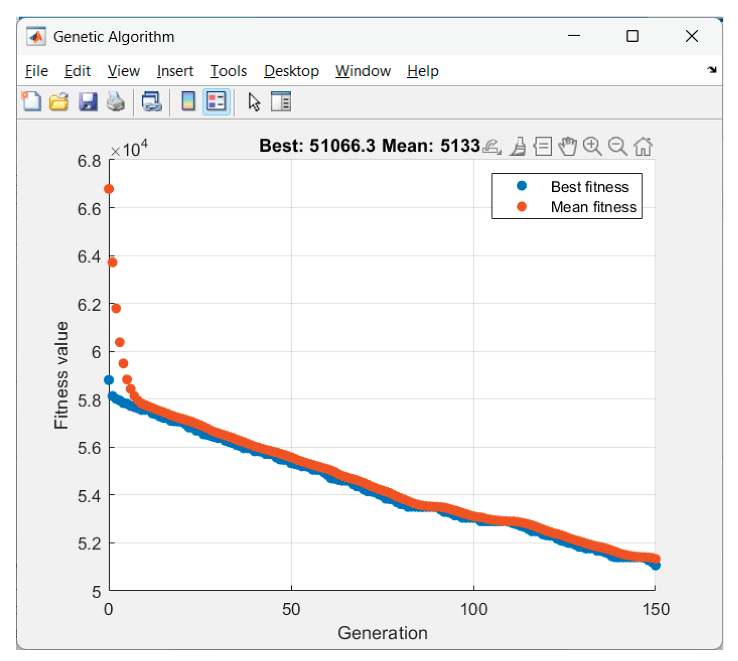
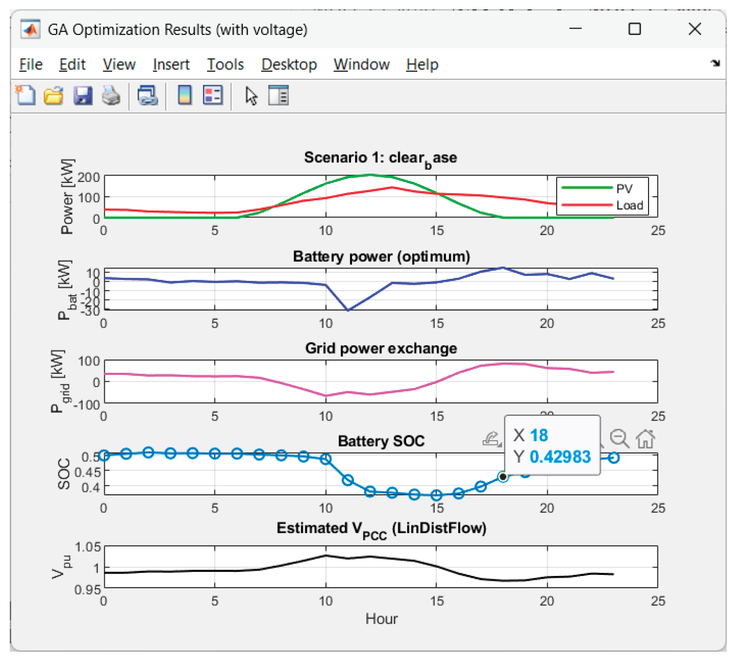
Figure 9.
Graphics for Scenario 1.
Received results from the GA-optimization of Scenario 2 ("thin_clouds"):
Figure 10.
GA performance in Scenario 2.
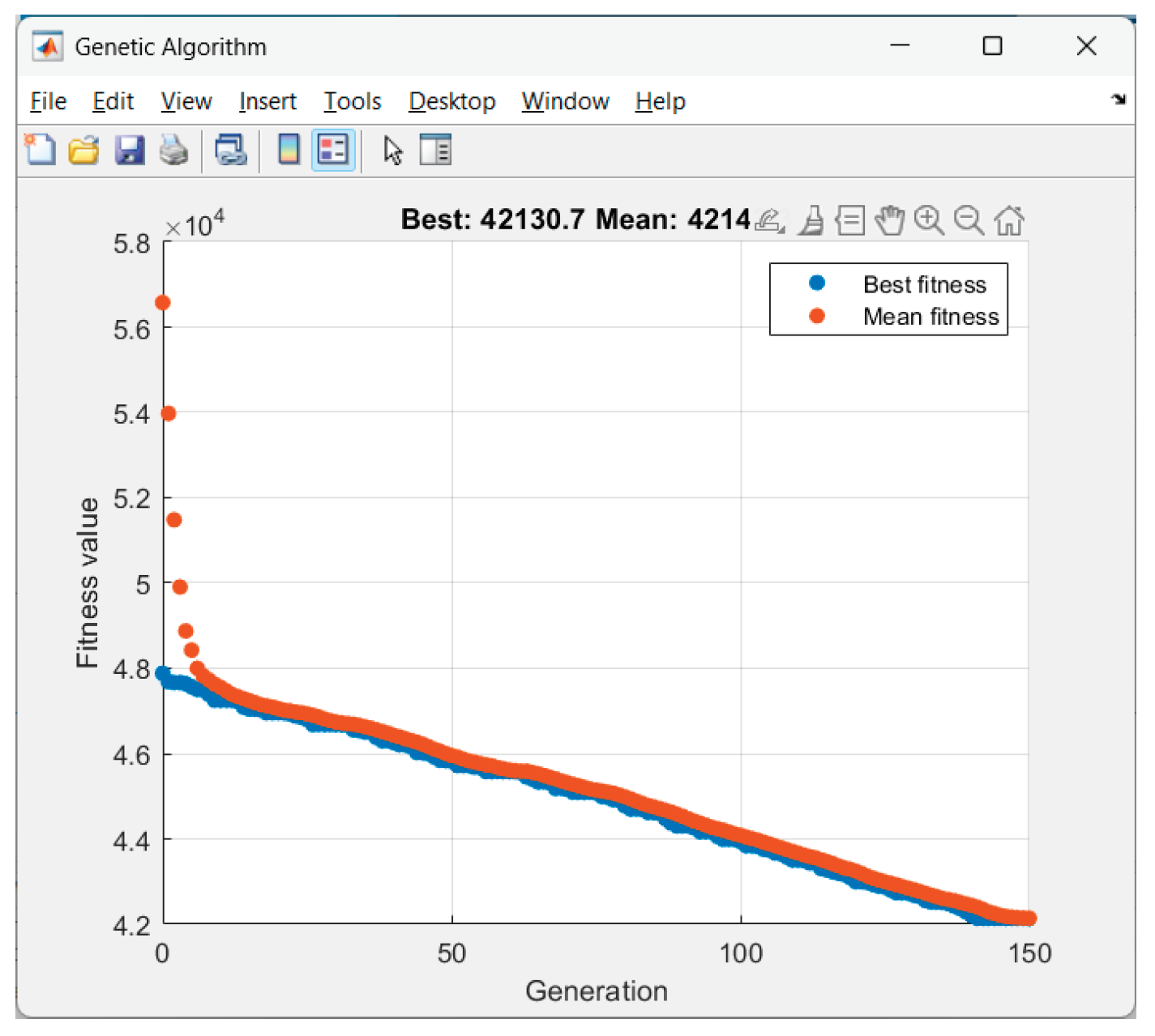
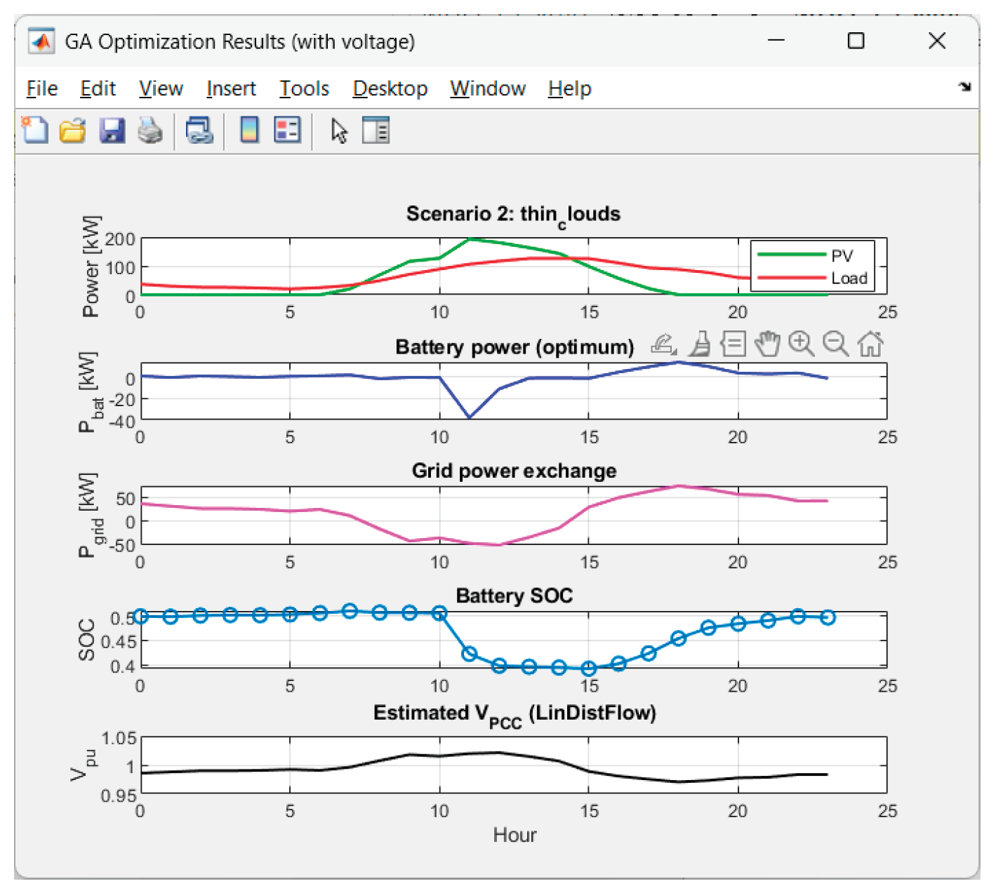
Figure 11.
Graphics for Scenario 2.
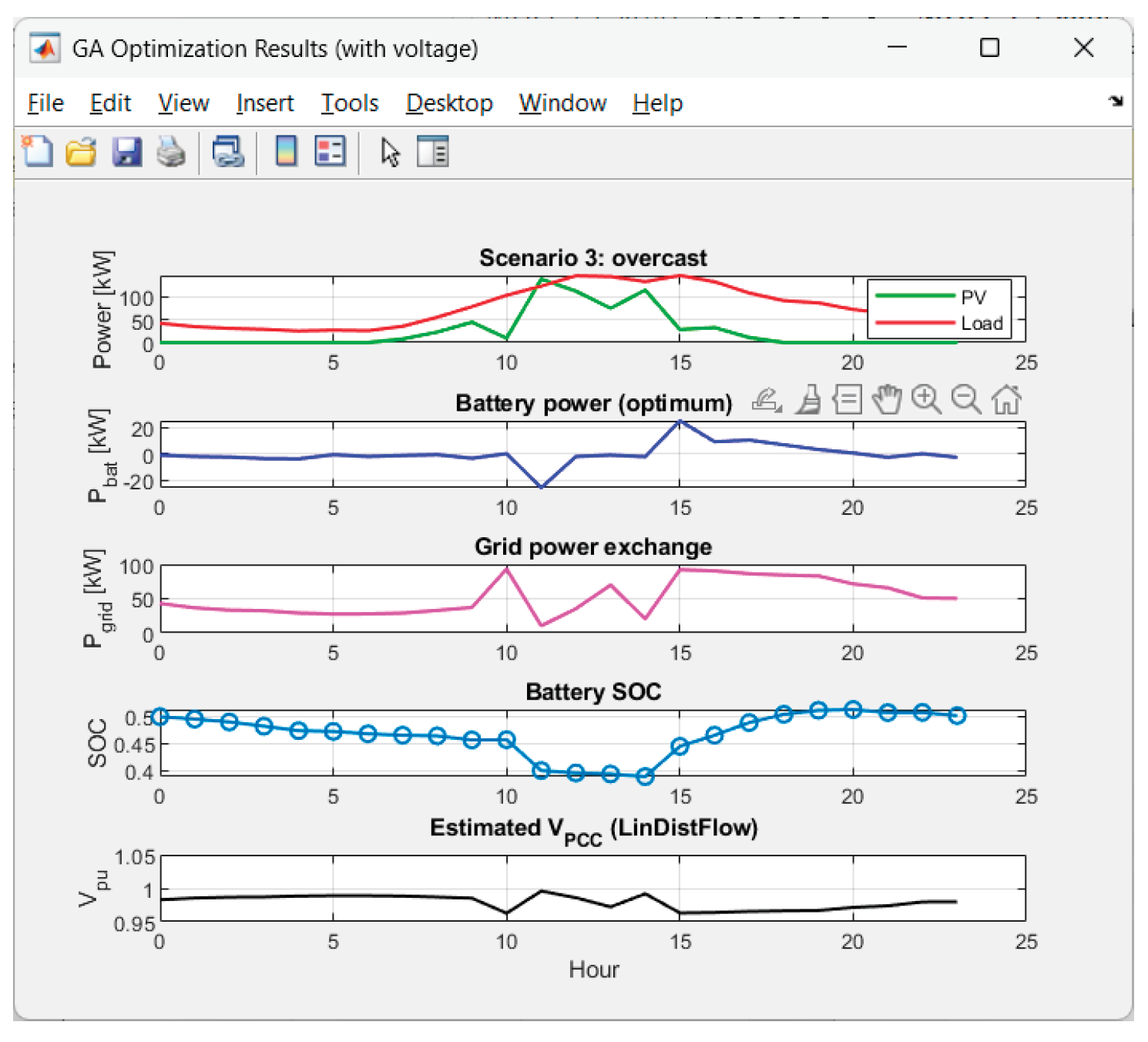
Received results from the GA-optimization of Scenario 3 ("overcast"):
Figure 12.
GA performance in Scenario 3.
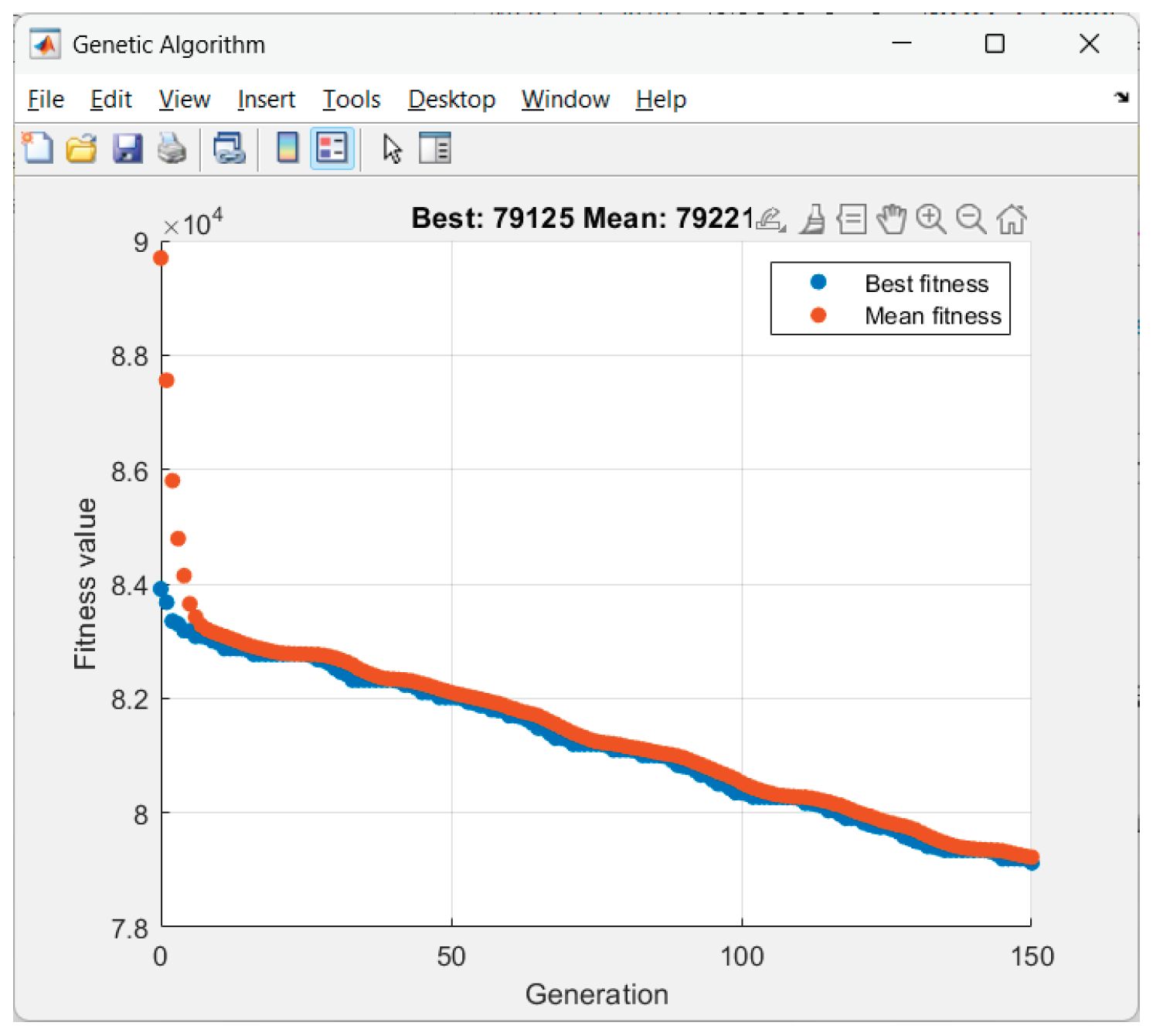
Figure 13.
Graphics for Scenario 3.
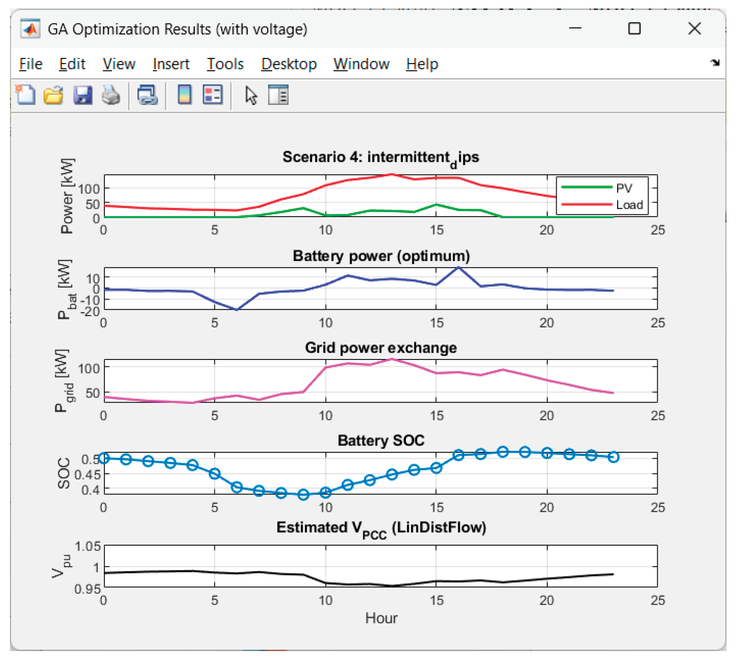
Received results from the GA-optimization of Scenario 4 ("intermittent_dips"):
Figure 14.
GA performance in Scenario 4.
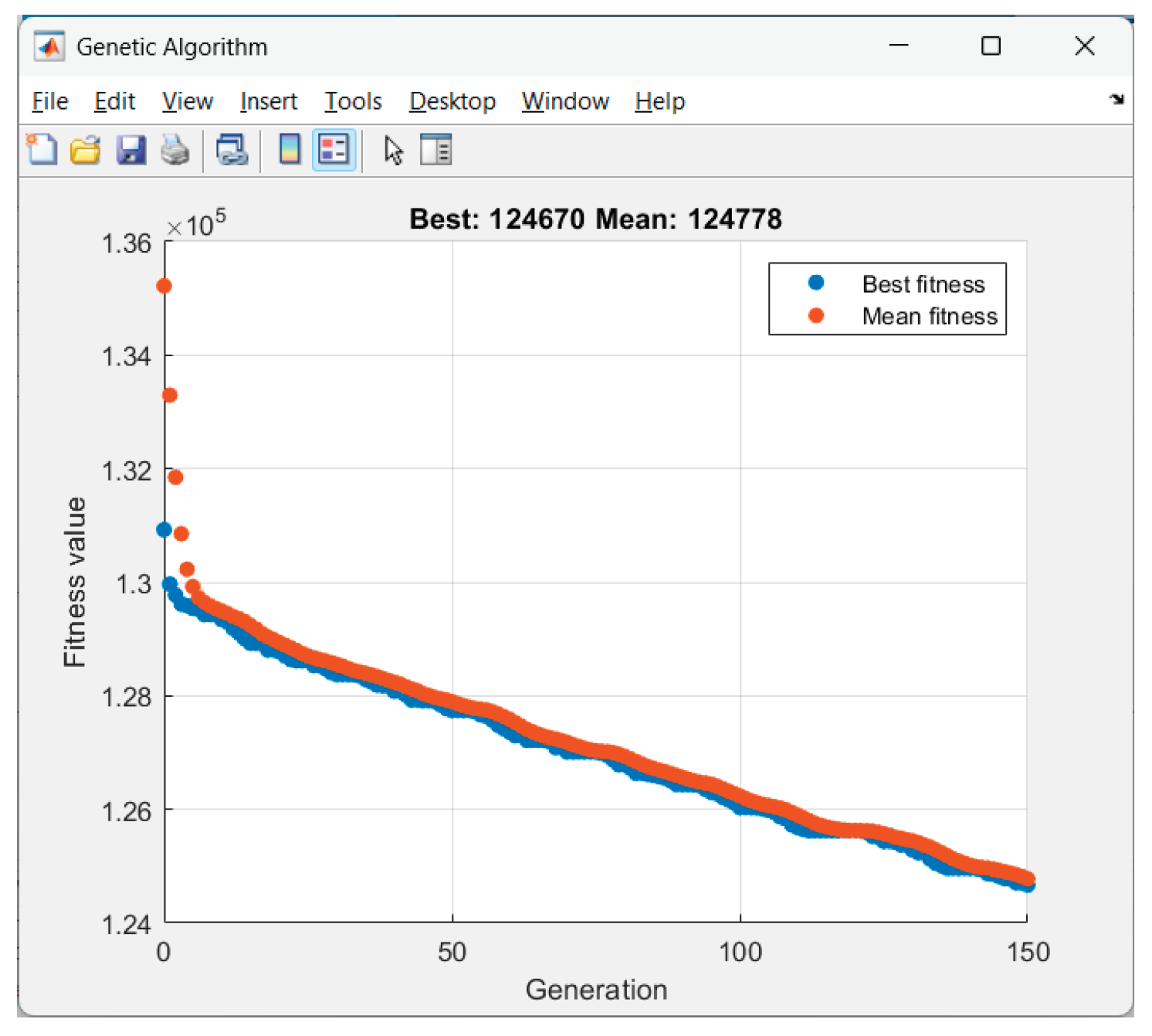
Figure 15.
Graphics for Scenario 4.
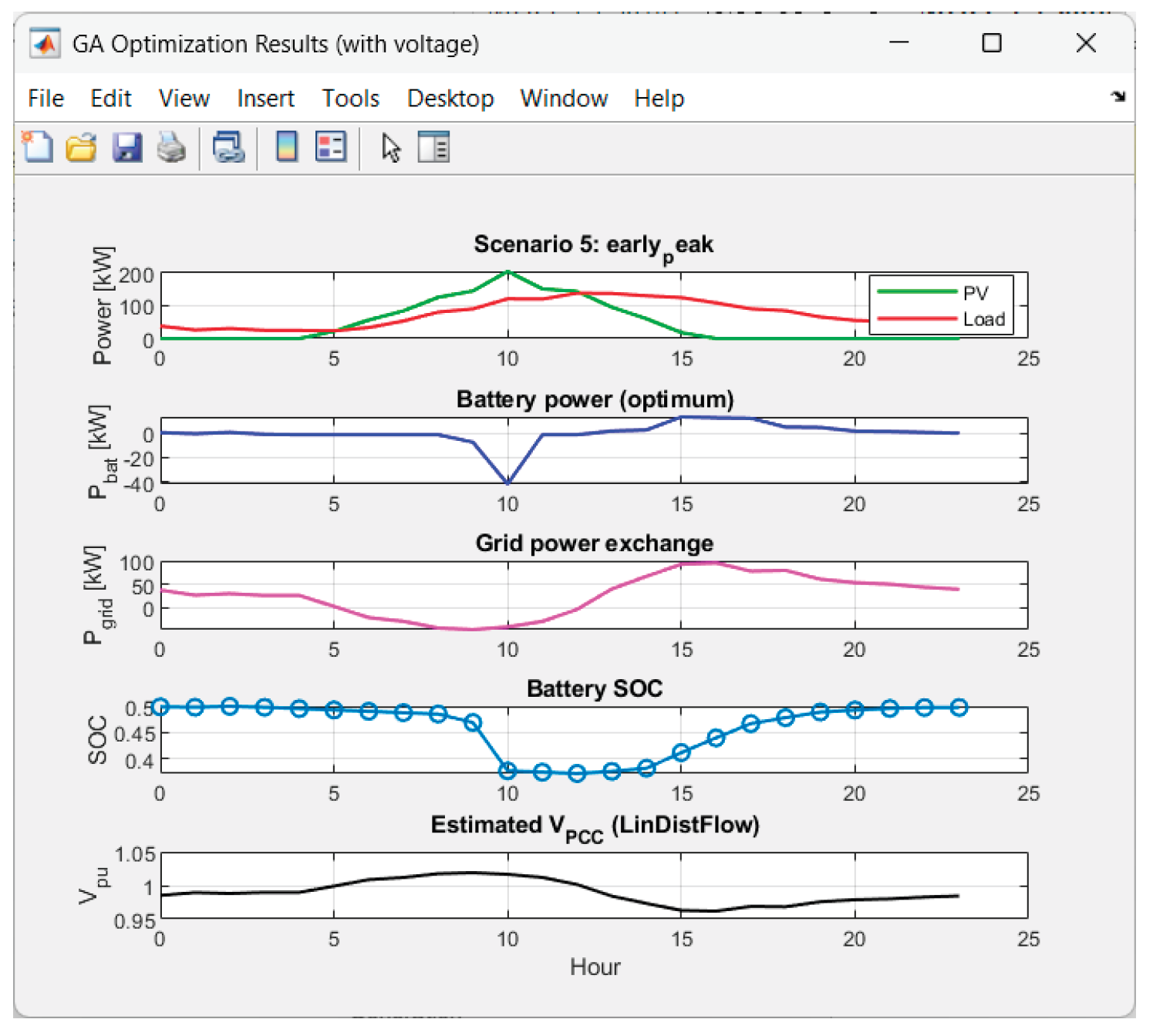
Received results from the GA-optimization of Scenario 5 ("early_peak"):
Figure 16.
GA performance in Scenario 5.
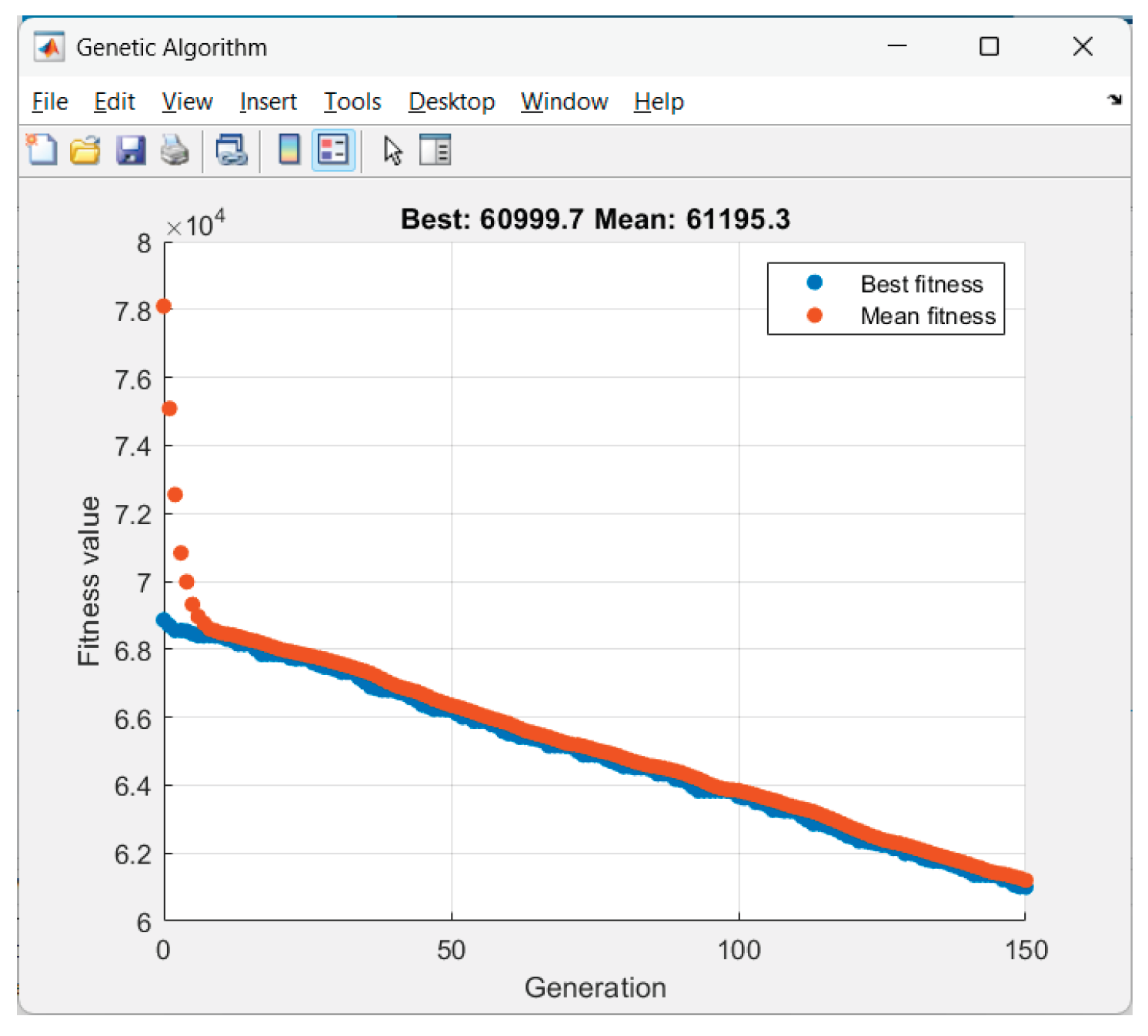
Figure 17.
Graphics for Scenario 5.
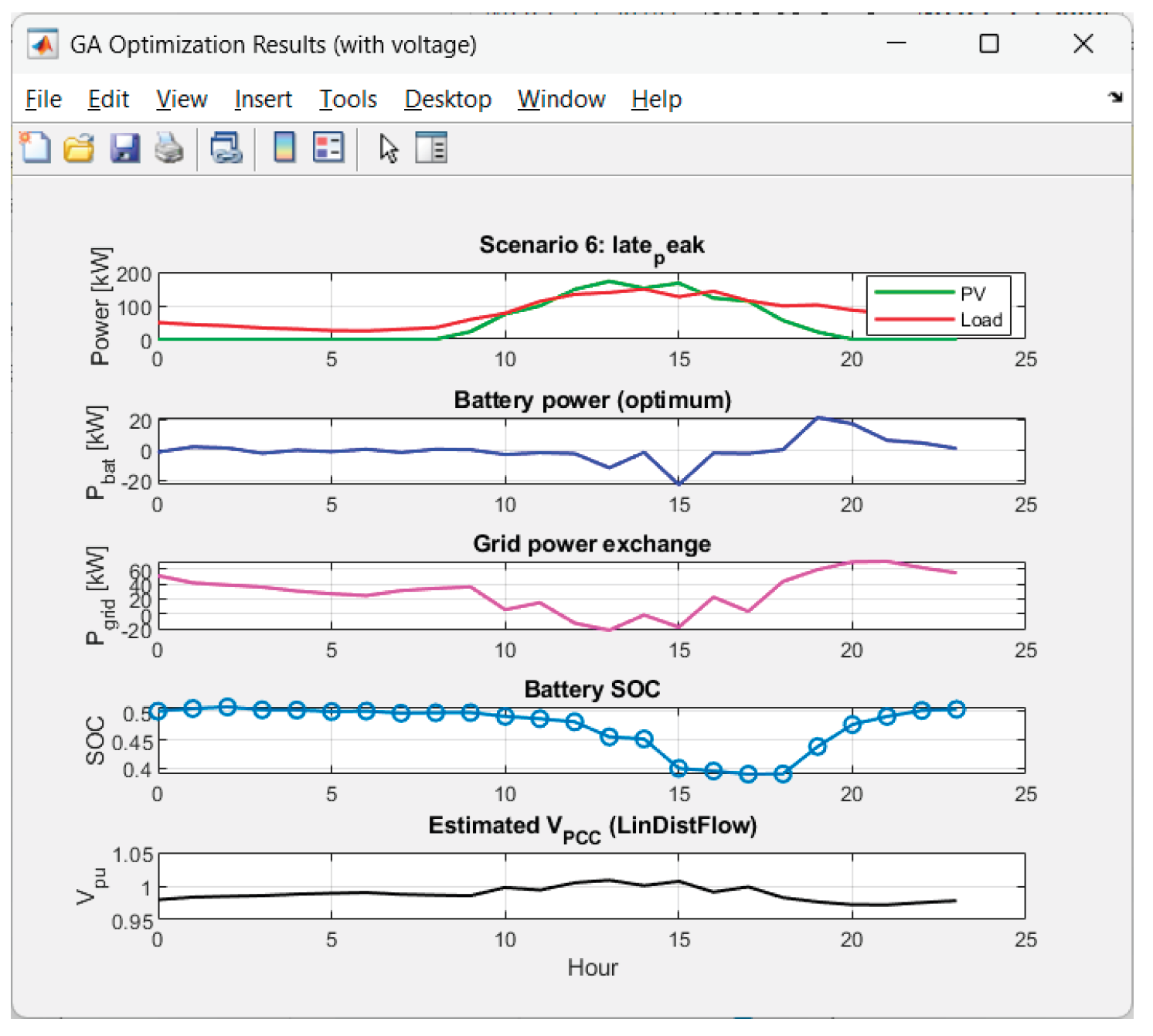
Received results from the GA-optimization of Scenario 6 ("late_peak"):
Figure 18.
GA performance in Scenario 6.
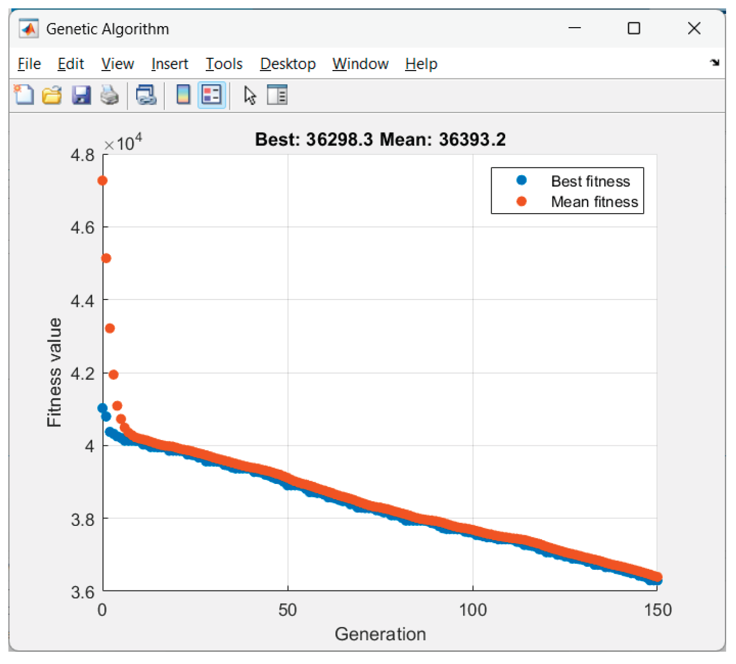
Figure 19.
Graphics for Scenario 6.
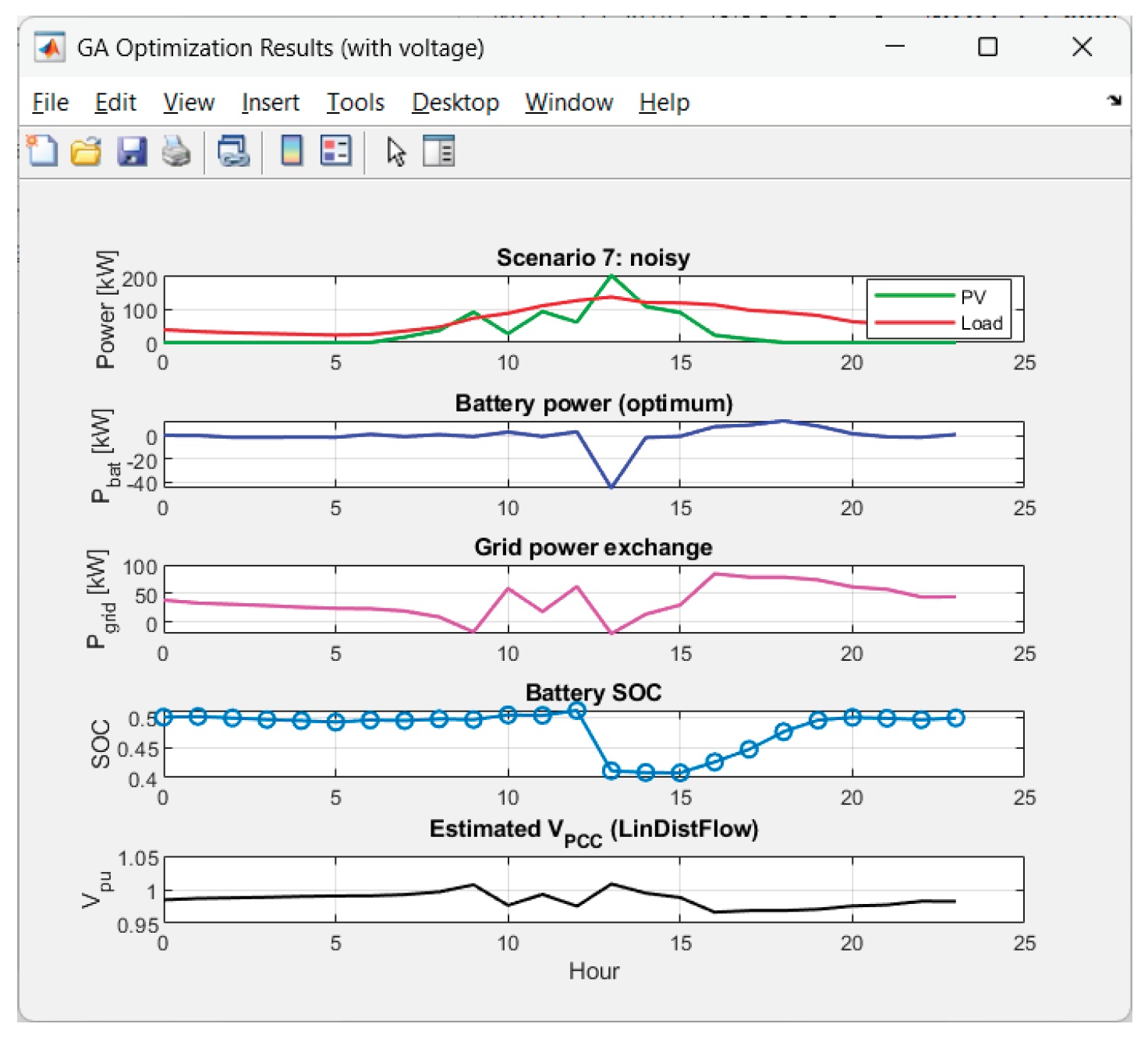
Received results from the GA-optimization of Scenario 7 ("noisy"):
Figure 20.
GA performance in Scenario 7.
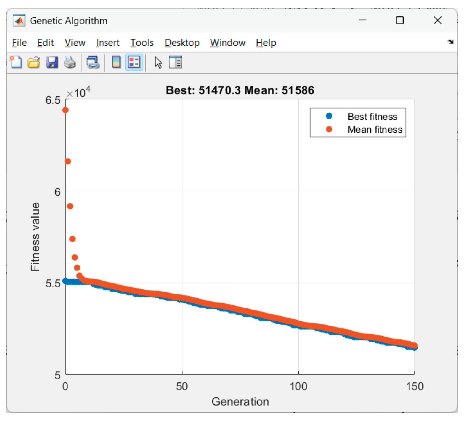
Figure 21.
Graphics for Scenario 7.
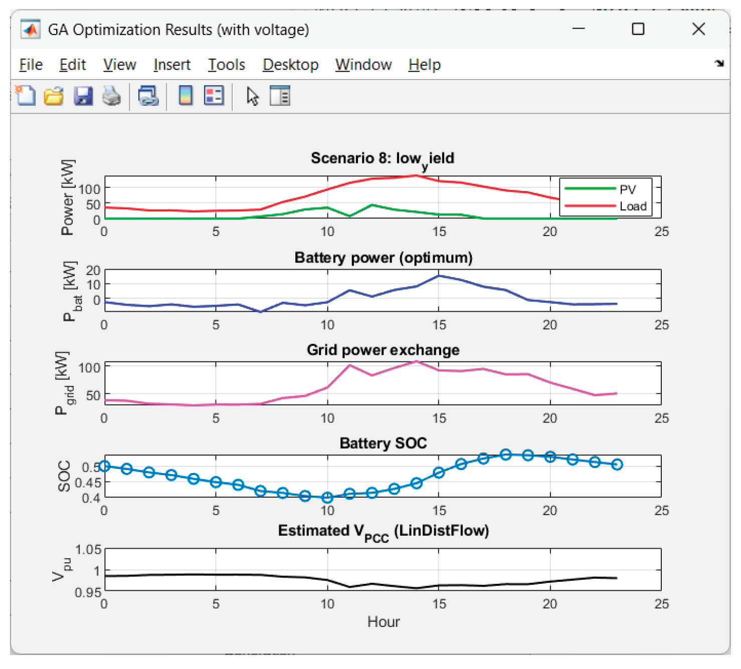
Received results from the GA-optimization of Scenario 8 ("low_yield"):
Figure 22.
GA performance in Scenario 8.
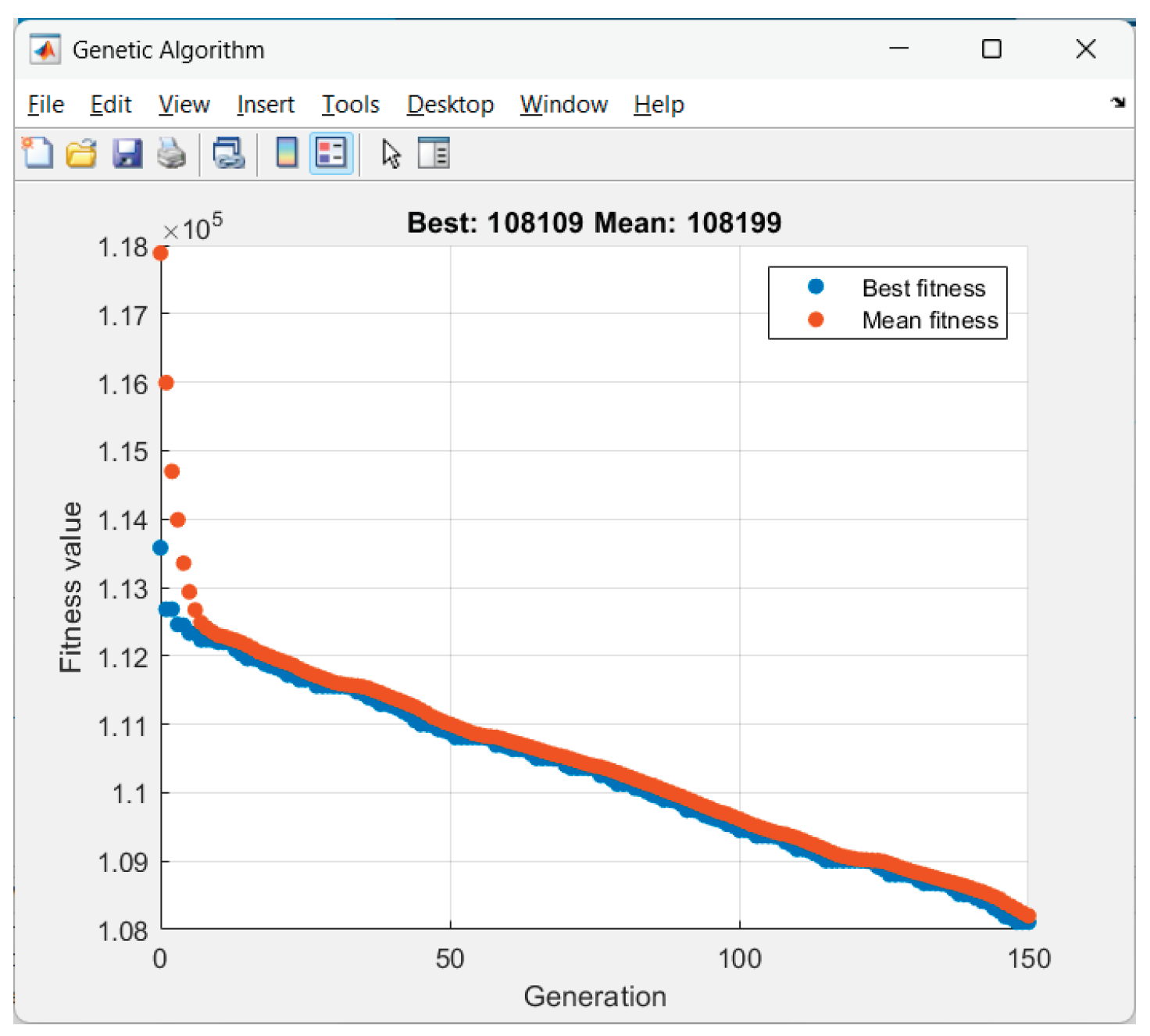
Figure 23.
Graphics for Scenario 8.
5.1. Analysis of Results from the Static Optimization
The voltage has excellent behavior. The performance results in 0% time outside the deadband for all 8 scenarios. Hence the combination deadband penalty + linear model performs very well.
The voltage deviations are small: max|ΔV| ~ 2.8%–4.5% pu; std(V) is small (0.010–0.018). Hence there is a smooth voltage profile, without flicker.
Energy balance and price:
• Most expensive scenarios in Energy_cost_USD are:
intermittent_dips ($174.68), low_yield ($161.86), overcast ($131.72).
These are intuitively the “bad weather” cases: low/unstable PV energy generation. Hence the purchase of energy during expensive hours is high.
• Cheapest: thin_clouds ($65.62) and clear_base ($67.76) → stable PV energy generation and/or harmony with tariffs.
• The asymmetry + tariff reduce the values of JGA compared to the purely symmetric version, because we severely penalize purchases (square, weight and price), and the energy selling is less penalized. This is desirable.
Battery throughput is ~99–139 kWh/day. At 450 kWh capacity this is reasonable (0.22–0.31 cycles/day equivalent, roughly). There are not available any "overpumping" or unnecessary oscillations. Hence the throughput is well balanced.
Pgrid_mean:
• On “good” PV days (clear_base, thin_clouds) the average Pgrid drops to ~16–17 kW and there is a net selling (Egrid− is significant).
• On “bad” days (intermittent_dips, low_yield) the average Pgrid is 61–66 kW and Egrid− ≈ 0. Hence the energy purchase cost is high.
• The scenario “late_peak” has a decent price result ($69.75) despite an average Pgrid ~29 kW — suggesting optimal shift of charging to nighttime cheap hours ($0.062) and discharging during the day.
5.2. Conclusions About the GA Performance
The objective function (19) performs exactly as intended: voltage safety, minimizing purchases during expensive hours, smooth profile, well SOC balance.
The cost distribution by scenarios matches the intuitive difficulty of the weather profiles.
6. Intelligent Control Applying Reinforced Learning – Training of the SAC Agent
6.1. Concept and Function of the Agent
In the Reinforcement Learning (RL) systems, the agent is an intelligent controller that makes decisions by interacting with the environment. The agent seeks to minimize deviations from the desired state through maximization of a negative reward.
At each step t:
- ➢
- The agent observes the state of the environment st (in our case: PV power, load, SOC and time).
- ➢
- It chooses an action at (here: active and reactive power of the battery).
- ➢
- The environment returns a reward rt and a next state st+1.
- ➢
- The agent updates its policy so that in the future it maximizes the expected total reward.
Let now us consider a Soft Actor–Critic (SAC) agent. SAC is a modern off-policy algorithm that combines:
• stochastic policy (for exploration),
• double Q-scoring (for stability),
• and entropy regularization (for balance between exploration and exploitation).
SAC agent consists of three main neural networks:
1. Actor (π) — a policy that proposes actions.
2. Critic 1 (Q₁) and Critic 2 (Q₂) — two independent estimates of the utility of actions.
They are used to avoid overestimation (Q-bias), typical in other RL methods.
The Actor network (πθ) generates actions based on the current state of the system.
This is the “brain” of the agent, telling “how much power to charge/discharge” and “what reactive load to compensate”. This network has a stochastic Gaussian Policy:
where
at = tanh(μθ(st) + σθ( st).ε), ε ~ N(0,1)
- μθ(st) is the neural network output for average value;
- σθ( st) is the dispersion (log-standard deviation);
- tanh ensures actions limits in the interval [—1, 1].
For one and the same state the agent does not return a fixed value, but a probability distribution:
At the beginning there is a high variance (exploration), and as training progresses — lower (exploitation).
Both critics (Q₁, Q₂) evaluate the quality of the chosen action in a given state — how “good” the actor’s choice is.
Each critic is a neural network that approximates the function:
for i = 1,2.
A single critic tends to overestimate the values Qi(st, at), which can lead to unstable learning. For this reason SAC uses Double Q-scoring avoiding systematic overestimation, and the agent learns more reliably.
Critics are trained by minimizing MSE:
where the objective is:
with α - “temperature” coefficient, controlling the compromise between the maximum reward and the entropy (diversity).
yt = rt + γ[min(Q1’, Q2’) − α.logπ(at+1|st+1)],
3. Value Target Network – used to stabilize the learning process.
Main hyperparameters of the SAC-agent are presented in Table 3:
Agent training is conducted offline in MATLAB RL Toolbox for 250–1000 episodes of 24 steps (hours).
Agent actions at each step (decision cycle):
1. Observes the vector state:
2. Actor proposes an action at = [].
3. The environment returns:
∙ new state st+1,
∙ reward Rt.
4. The critics calculate Q1(st,at) and Q2(st,at).
5. The agent updates:
∙ the critics (by TD-error between predicted and actual Q-score).
∙ the actor, so that it chooses actions with higher Q-score and higher entropy.
In our case, the Actor regulates Pbat and Qbat (charging/discharging, compensation). Critics (Q₁, Q₂) evaluate how “good” this strategy is, taking into account the reward, SOC, and the exchange with the network. After enough episodes (in our case 350), the Actor learns to choose actions that minimize the quadratic cost in Reward, i.e. to maintain SOC close to 0.5.Cbat,max and minimum power exchange with the main grid Pgrid, ensuring optimal energy balance.
The flowchart of the SAC agent is presented in Figure 24.
6.2. RL – Training of the SAC Agent
The objective of the SAC agent is to minimize the deviations from the desired state through maximization of a negative reward function.
For the step t (with Δt = 1 h), it is ∈defined:
Pgrid(t) = Pload(t) – Ppv(t) – Pbat(t)
Qgrid(t) = Qload(t) – Qbat(t) , (here Qpv(t) = 0)
P+ = max(Pgrid(t),0), P− = max(−Pgrid(t),0)
PF limit: |Qgrid(t)| ≤ tan(arccos(pfmin))|Pgrid(t)|
Violation Qviol = max{|Qgrid(t)|− tan(arccos(pfmin))|Pgrid(t)|, 0}
For each step t is added a voltage term Vpu(t) (per-unit). It corresponds to in (16). It is useful to work with a dead band (e.g. [Vmin,Vmax]=[0.95, 1.05] pu), i.e. we penalize only deviations outside the allowable zone.
At Point of Common Copuling (PCC):
Sbase is the microgrid rating.
Smoothness: ΔV =
Normalized State of Charge: , goal sf = ;
The reward function used for reinforced learning of the agent is defined as follows:
where:
R(t) = R1(t) + R2(t)
The “–” sign in front of the brackets in (26, (27) means that the agent maximizes the reward, equivalent to minimizing the quadratic penalties inside.
wP (dimensionless) is the weight of the active power component. The larger it is, the more the agent minimizes the exchange of active power with the network. In our experiments we assume wP = 1.0. In case more aggressive power economy is desired, a greater value of wP can be used, for example wP ∈[2.0, 3.0].
wQ (dimensionless) is the weight of the reactive power component. It promotes maintaining good cos φ and limiting Qgrid. In this study it is assumed that wQ = 0.1.
wSOC (dimensionless) is the weight of SOC deviation from the center (50% or 0.5). In case of a higher value, it leads to more conservative behavior (smaller SOC fluctuations). Its lower value leads to more active battery. In this study it is assumed that wSOC = 0.1. The idea here is to penalize SOC deviations more strongly and stabilize battery behavior.
c(t) is the hourly energy price; [x]+=max(x,0) only penalizes the power consumption from the main grid.
is the penalty for SOC < 0.2 or SOC > 0.9 to avoid aggressive charging/discharging.
7. Results from the RL – Training of the SAC Agent
Eight different scenarios were generated for typical solar-temperature conditions:
1. Clear base, 2. Thin clouds, 3. Overcast, 4. Intermittent dips, 5. Early peak, 6. Late peak, 7. Noisy, 8. Low yield.
Each scenario includes 24-hour PV and load profiles that are fed to the training environment (see Figure 4 and Figure 5). This provides enough variety to evaluate the generalization ability of the SAC agent.
For each scenario “Penalty breakdown” graphics as those in Figure 25 are received. The hourly rate for electricity is denoted by TOU = ”Time-of-Use” price. In (26), "TOU price" is the array c(t) [$/kWh] for each hour t=1,...,24;
Example of the reward function is shown in Figure 26.
The training of the SAC agent aims to bring the Reward function values close to 0. This will mean that it has learned to provide a stable energy management policy that adapts to different PV and load profiles. After some tuning of parameters and performing several experiments, it was assumed that 350 learning episodes are enough for training the agent in each scenario. Below are presented graphics of Episode Q0, Episode reward, and Average reward for the agent training in the different scenarios:
Figure 27.
Agent training in scenario 1.
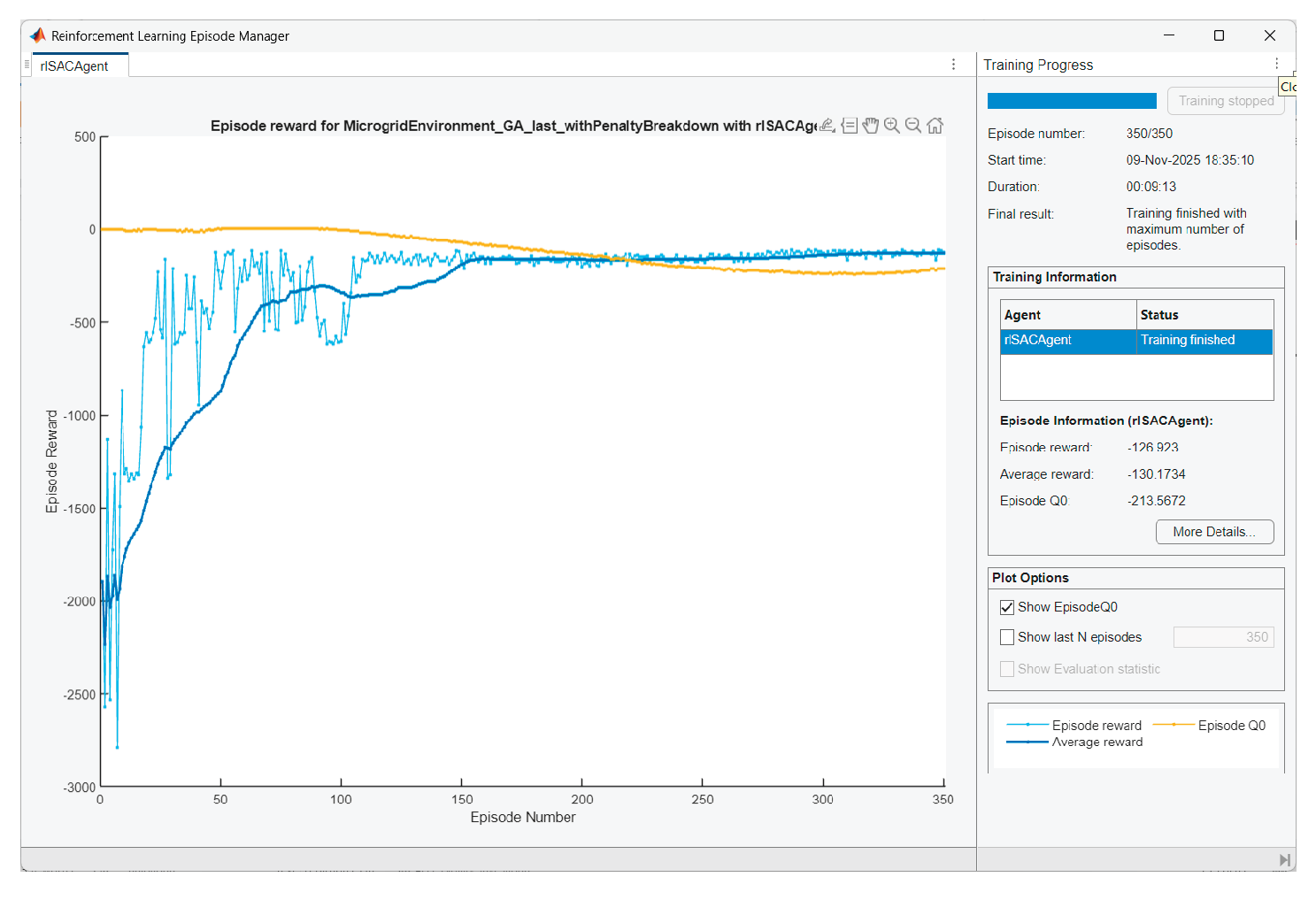
Figure 28.
Agent training in scenario 2.
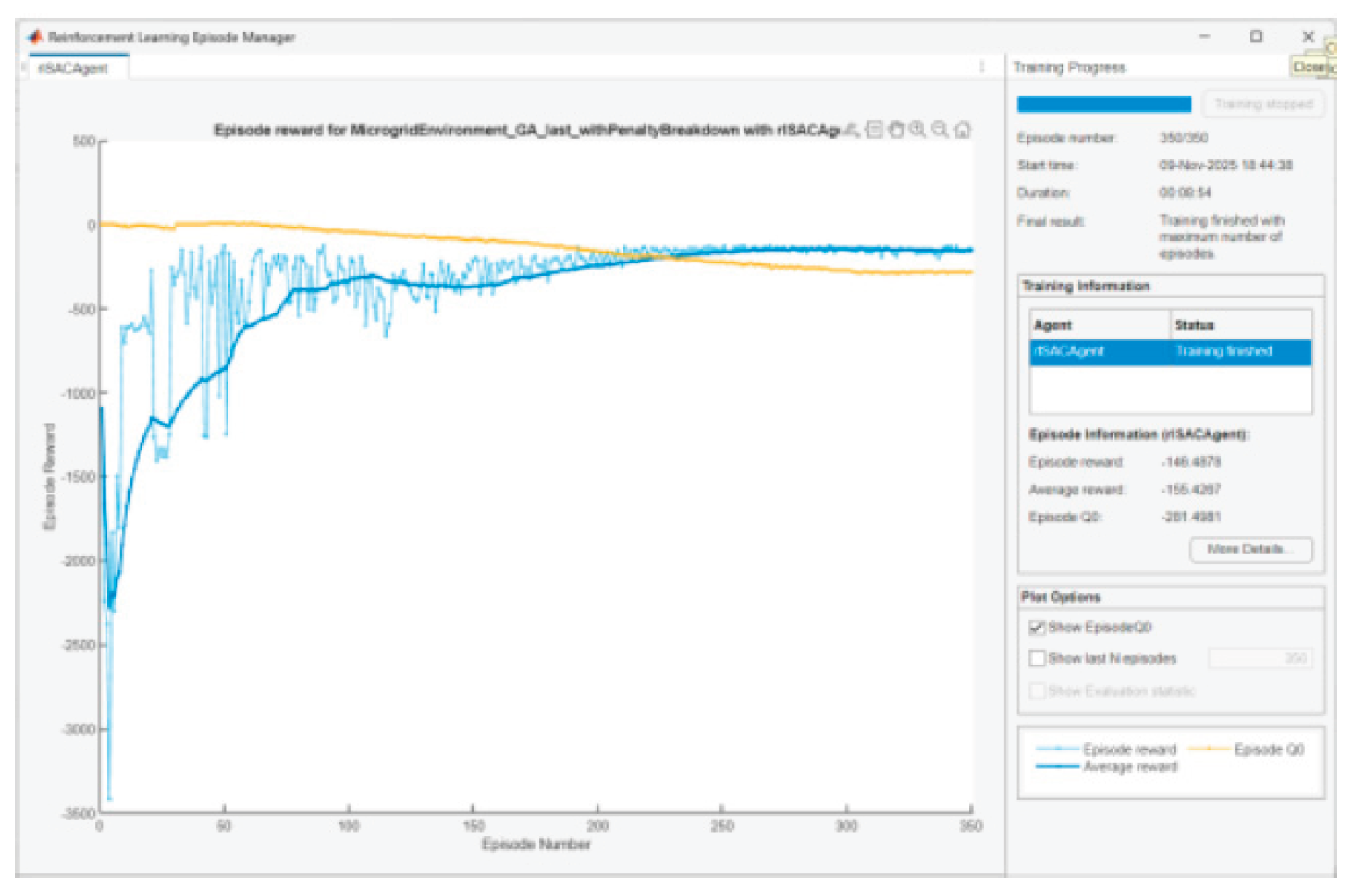
Figure 29.
Agent training in scenario 3.
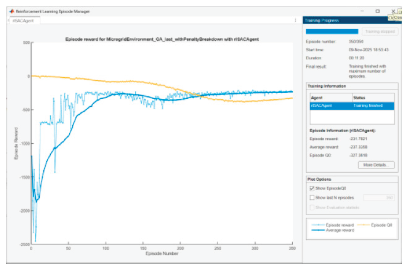
Figure 30.
Agent training in scenario 4.
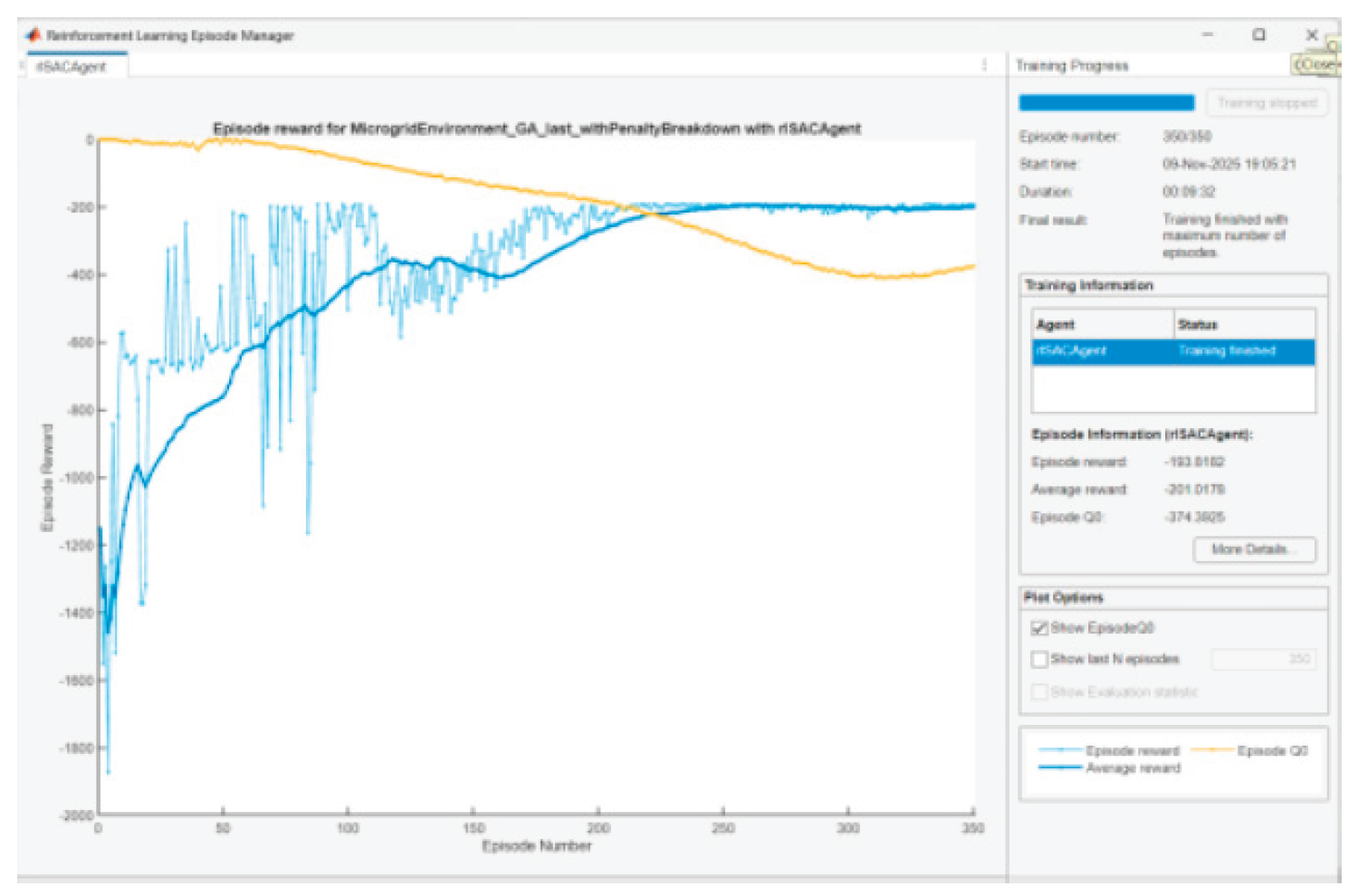
Figure 31.
Agent training in scenario 5.
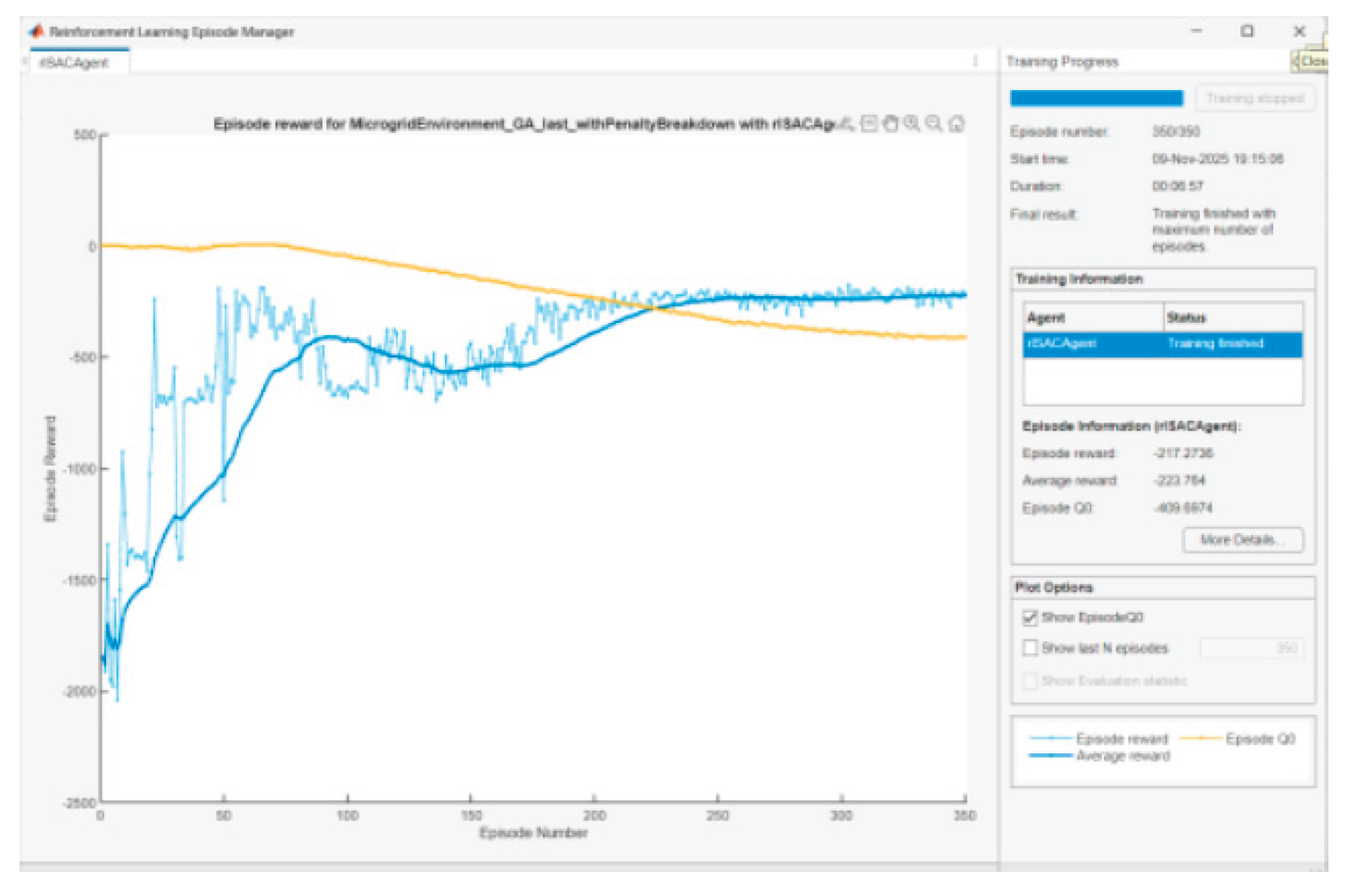
Figure 32.
Agent training in scenario 6.
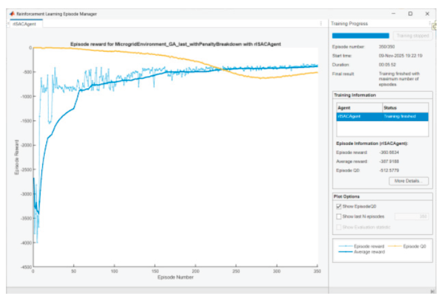
Figure 33.
Agent training in scenario 7.
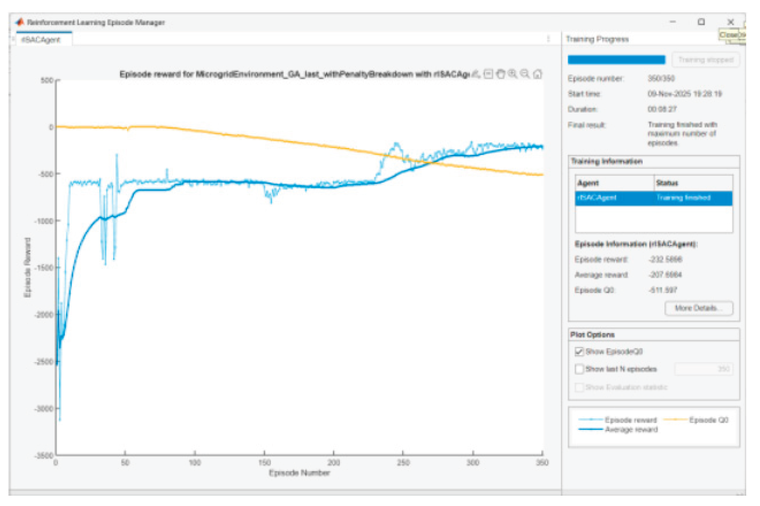
Figure 34.
Agent training in scenario 8.
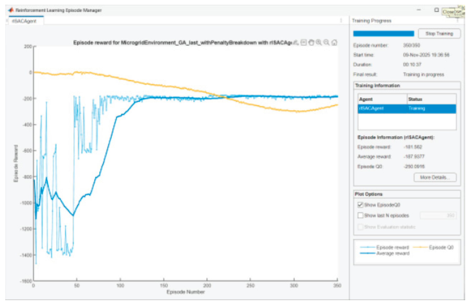
The question arises: Why Episode reward ≠ Episode Q0?
• Q0 is a critic’s estimate of the expected accumulated reward at the starting state, with stochastic policy and entropy included.
• When the entropy coefficient is significant and/or critics slightly overestimate/underestimate, there will be a gap. We are looking for convergence with episodes, not complete coincidence. The observed convergence after 350 episodes is normal.
In SAC Episode Q0 is an estimate of the initial Q-value from the critic(s); Reward is the actual total reward. The difference remains because (i) the Q-estimators are approximate; (ii) we have a stochastic actor + entropy; (iii) there is a terminal SOC term at the end that is not perfectly “predictable” by Q in early episodes. It is normal for Q0 and average reward to be parallel with a small constant difference.
The received results are summarized in Table 4:
Results for the Average reward per Scenario are presented in Figure 35.
8. Training Results Analysis
8.1. General Observations
• Convergence: With 350 episodes training all scenarios give small average penalties (AvgReward ~ −5…−15). This means that the agent has stabilized its policy and is “standing” close to a reasonable strategy.
• Dominant terms: Analysing “penalty breakdown” graphics, the Price term () is the largest contributor almost everywhere, and ΔV-term (Voltage smoothness) is the second most important in cloudy/noisy profiles. Penalties for V (dead band), Qviol, P− and SOC are low. Hence constraints are well satisfied / respected. In all scenarios, Price (TOU) and ΔV-term are leading. This explains why in “clear” profiles (Clear base, Thin clouds) the average reward may be worse — cheap nighttime electricity + large daily voltage dynamics push the agent towards specific behavior (more night time charging and smaller/slower changes during the day), which does not match the GA profiles.
• Difference between Average reward and Final reward: Considering scenario 7 (“Noisy”) Final reward is the last episode reward and may be “bad luck” (noise/exploration).
• “Low yield”-scenario: Almost all the “cost” comes from Price-term — logically, because PV energy generation is low and the system rarely violates voltage, and ΔV is small.
• Scenarios “Noisy” / “Overcast”: ΔV and Price are close in scale → the agent balances both, so the average reward is moderately negative, not the worst.
8.2. Analysis by Scenarios
1. Clear base (Average reward: −5.09, Final reward: −4.15)
The easiest profile gives a small price/penalty. The agent causes charging at a cheap time and discharging when it is necessary. Good behavior.
2. Thin clouds (Average reward: −6.54, Final reward: −2.99)
Slight variability introduces a little more ΔV and slight errors in the loading timing, but the price term in the reward remains dominant. The final reward is excellent (−2.99) — the last episode is strong.
3. Overcast (Average reward: −9.60, Final reward: −4.03)
Low PV generation → more energy import → Price grows. The agent limits ΔV, but the price “pulls” down the average reward.
4. Intermittent dips (Average reward: −7.99, Final reward: −3.33)
Short “holes” in PV generation → jumps in ΔV and short increases in import prices. Nevertheless, the finale is decent.
5. Early peak (Average reward: −10.01, Final reward: −4.38)
Early day load/price requires pre-charging at night. Probably the agent doesn't store enough energy for the early peak yet → SOC should be higher.
6. Late peak (Average reward: −14.45, Final reward: −3.99) — the hardest
Late evening peak in the expensive zone → if SOC is low in the afternoon, energy from the main grid should be bought expensively. This explains the worst Average reward. A greater "energy reserve for the evening" is needed.
7. Noisy (Average reward: −9.15, Final reward: −24.86)
Average does well, but the last episode is bad (probably higher stochastics/exploration). In evaluation mode (without stochastics) the result is usually better.
8. Low yield (Average reward: −7.51, Final reward: −8.71)
Little PV generation → price term in the reward dominates, but there are no problems with voltage/limits. The agent behavior is adequate.
8.3. Root Mean Square Error (RMSE) Metrics
Two root mean square errors will be considered.
- ➢
- Root Mean Square Error (RMSE) for SOC
Let:
T be the number of time steps (e.g. 24 for 24 hours);
SOCGA(ti) — normalized state of charge from the GA model at time ti;
SOCRL(ti) — normalized state of charge from the RL simulation at the same time.
Then RMSE for SOC is calculated as:
When RMSESOC = 0, there is full match between GA and RL. When RMSESOC = 1, there is complete divergence (maximum possible, since SOC is normalized in [0,1]).
- ➢
- Root Mean Square Error (RMSE) for active power to the grid
Similarly, if:
is the active power to/from the grid in GA optimization [kW];
is the same quantity obtained from the RL agent;
T is the number of steps;
then:
Both root mean square errors should be considered here as a diagnostic metric, not as a goal. GA and RL optimize different functionals (even with close weights): RMSEPgrid and RMSESOC simply show how different the resulting policies are, not "which one is better".
Let we consider the comparison (GA vs RL) for the scenarios: 1. Clear base, and 4. Intermittent dips. The correspondent graphics are presented in Figure 36 and Figure 37.
In both scenarios:
• The curve is permanently negative and decreasing (≈ –20 → –60 kW). That is, RL leads the system to net export/low energy purchase from the main grid.
• SOCRL grows smoothly throughout the episode, while SOCGA stays almost flat around 0.5 (in Scen. 1) – both strategies are completely different.
• is a positive line (“charge - / discharge +”), which suggests discharging almost all day long.
In Scenario 1:
• Price dominates; there is a noticeable ΔV; V-deadband ≈ 0 (voltage stays within the limits); P+/P- are small after normalization.
• RL “chases” minimum purchase (Ppos), striving to make a profile that minimizes the price term; the different strategy from GA comes from the fact that RL optimizes price+voltage+smoothness, while the GA has a different goal.
In Scenario 4:
• Again Price-term is dominating; ΔV is second (the scenario has sharp PV drops → larger |ΔV|); the voltage remains in the deadband, so V ≈ 0.
• RL again pulls towards a profile with low purchase and smoother V, so it stays with Pgrid below zero and “smoothes” the dynamics.
Conclusion: RL does NOT imitate GA because the goals are not the same:
• GA aims to achieve optimal energy flow (good balance).
• RL aims to achieve optimal penalty according to Price and ΔV.
Analysis:
- A)
- RL ≠ GA, which is expected (different objective function)
GA optimizes:
- minimal deviation from real Pgrid (with direct objective: minimizing error)
- exact following of SOC requirements
- symmetric quadratic penalties
RL optimizes:
- minimization of assembled reward
- dominated by the price component
– RL minimizes energy bill.
– does not minimize the difference to GA profile.
RMSE does not measure RL error, but the “distance to the GA strategy”.
B) The most interesting thing: RL systematically keeps the battery “more discharged”
From the comparisons:
• SOCRL starts at ~0.05 instead of 0.5
• The battery in RL discharges throughout the day with ~30–40 kW
• This leads to
→ lower Pgrid (in absolute value)
→ strongly different SOC compared to GA → large RMSE
This is a rational solution for the RL agent because:
RL minimizes PricePenalty, not trajectory-tracking penalty.
At high evening tariff
→ RL tries to keep the battery as full as possible.
→ therefore there are “overcharges” every morning, leading to different SOC.
C) The largest RMSEs (Pgrid & SOC) occur at scenarios:
• Overcast
• Intermittent dips
• Low yield
• Noisy
This is where GA and RL react the most differently:
• GA follows a “short horizon” (hour by hour)
• RL accumulates energy proactively when it is cheap
• At low PV production, RL becomes even more aggressive for early charging
Thus, the difference in SOC increases leading to worse RMSE.
D) Interpretation: What do RMSE values mean?
RMSEPgrid ≈23–33 kW (at 24 hours)
→ This is completely normal, because RL and GA have different strategies.
• GA keeps Pgrid close to balance.
• RL optimizes for minimum cost, not balance.
Therefore, RMSE for Pgrid is NOT an indicator of RL error.
It only shows the “distance between two different optima”.
RMSESOC ≈0.30–0.44
→ This is a big discrepancy.
But it is also logical:
• RL always follows a price motive – loads when it is cheap
• GA follows a trajectory-constraint – keeps SOC close to a planned line.
Again — different goal → different profiles → different SOC.
E) General state of the agent
• RL makes “economically” optimal decisions
In all scenarios, PricePenalty is the largest term (3–6 times larger than all others).
The agent is trained to:
1. Reduce evening grid consumption
2. Charge the battery early (even when GA does not)
3. Avoid reactive limits (Qlim ≈ 0 always)
4. Never goes outside SOC_min / max limits
No technical violations — this is a strong indication of a stable controller.
RL shows a consistent strategy across all 8 scenarios
Two different types of behavior:
• Scenarios 1–2 (high sun): RL charges moderately
• Scenarios 3–8 (low sun): RL starts charging aggressively from the start
This is ecologically valid, economically optimal, and stable.
F) Summary: How does the RL agent perform?
- ➢ Good behavior
• The strategy is stable and scenario-independent
• Prefers early charging
• Strictly respects SOC limits
• Keeps Pgrid lower in high-tariff intervals
• Reactive component always under control
- ➢ RMSE is not an indicator of error, but of a difference in strategy
That's exactly what we wanted - RL does not imitate GA (keeping Pgrid close to balance), but optimizes the economy.
RL and GA have different goals, which leads to different optima.
9. Conclusions
This work proposes a new integrated approach to the optimization of energy management in microgrids by combining heuristic methods (Genetic Algorithm, GA) and reinforcement learning methods (Reinforcement Learning, RL), the contribution of which can be summarized as follows:
1. Development of a new, physically plausible RL environment for microgrid control
An advanced reinforcement learning environment is presented, which includes:
• battery dynamics with SOC constraints, bidirectional flow and inverter limits (P–Q–S);
• linear approximation of the distribution network via the LinDistFlow model;
• active and reactive flows between the microgrid and the main grid;
• temporal context via a normalized hourly index.
• two-tariff price signals (TOU) and their nonlinear effects.
• multiple penalty terms addressing voltage deviations, inverter capacity overruns, economic losses and irregular SOC trajectories.
This design represents a significant advance over standard RL environments in the literature, which often simplify electrical constraints or ignore them entirely.
2. Implementation of a multi-scenario training and validation platform
A library of eight realistic PV/Load scenarios has been developed, including:
• clear, partly and heavily cloudy profiles,
• early and late load peaks,
• noisy and volatile PV generation,
• days with low-energy generation.
The RL agent has been trained and tested on all scenarios, which provides robustness and generalization ability rarely demonstrated in existing scientific works.
3. New “Penalty Breakdown Framework” for RL Policy Interpretation
A new method for reward decomposition is presented, through which:
• each component of the reward function (Pgrid, Price, ΔV, SOC drift, Q overflow, etc.) is tracked individually;
• its influence is averaged over time steps and scenarios;
• what the agent actually “learns” and which factors dominate its behavior is visualized.
The methodology creates high interpretability of RL actions and allows for more precise settings of the reward structure.
4. Development of a unified methodology for comparison between GA and RL
A new technique for direct comparison between GA and RL is proposed:
• reconstruction of RL actions.
• denormalization and re-simulation of the system equations.
• automatic calculation of RMSE for Pgrid and SOC;
• comparison between “optimal” GA and “scientific” RL control.
This contribution is significant, as it allows for quantitative measurement of the differences between analytically optimal behavior (GA) and behavior acquired through training (RL).
5. Empirical result: RL learns a different but robust strategy compared to GA
The experiments show:
• 24–33 kW RMSE for active power to the grid.
• 0.30–0.44 p.u. RMSE for SOC.
• RL does not replicate the GA-profiles, but develops an alternative robust strategy based on minimizing TOU costs and voltage disturbances.
• robust behavior in all scenarios, including noisy and low-energy ones.
This demonstrates that RL can serve as an adaptive controller that optimizes behavior under conditions of uncertainty.
6. First integrated GA ↔ RL framework for microgrids
The proposed experimental platform, combining:
• GA optimization,
• SAC agent,
• realistic scenarios,
• penalty breakdown,
• RMSE comparison,
represents a new scientific framework that can be directly used in future research works or industrial tests.

Table 6.
Data for PV system energy generation [kW] in the 8 scenarios (24 hours, 1 hour step).
| Scen. 1 | Scen. 2 | Scen. 3 | Scen. 4 | Scen. 5 | Scen. 6 | Scen. 7 | Scen. 8 |
| 0 | 0 | 0 | 0 | 0 | 0 | 0 | 0 |
| 0 | 0 | 0 | 0 | 0 | 0 | 0 | 0 |
| 0 | 0 | 0 | 0 | 0 | 0 | 0 | 0 |
| 0 | 0 | 0 | 0 | 0 | 0 | 0 | 0 |
| 0 | 0 | 0 | 0 | 0 | 0 | 0 | 0 |
| 0 | 0 | 0 | 0 | 22.074 | 0 | 0 | 0 |
| 0 | 0 | 0 | 0 | 56.090 | 0 | 0 | 0 |
| 23.465 | 20.347 | 7.695 | 6.086 | 84.068 | 0 | 16.427 | 6.852 |
| 67.295 | 69.241 | 22.858 | 17.453 | 125.208 | 0 | 36.783 | 14.409 |
| 117.167 | 115.817 | 44.357 | 30.388 | 144.575 | 22.475 | 92.243 | 29.614 |
| 162.061 | 126.814 | 9.457 | 5.894 | 204.0 | 74.485 | 26.630 | 35.420 |
| 192.992 | 193.329 | 138.136 | 7.019 | 150.904 | 99.199 | 94.105 | 7.715 |
| 204.0 | 180.799 | 111.951 | 22.194 | 142.968 | 148.284 | 61.689 | 44.007 |
| 192.992 | 163.435 | 74.642 | 20.997 | 95.261 | 172.419 | 204.0 | 28.994 |
| 162.061 | 143.544 | 114.342 | 17.632 | 60.062 | 152.053 | 109.417 | 21.472 |
| 117.167 | 98.391 | 28.504 | 42.838 | 18.090 | 166.916 | 91.002 | 13.033 |
| 67.295 | 56.783 | 32.615 | 24.604 | 5.131E-24 | 122.587 | 22.196 | 12.515 |
| 23.465 | 21.693 | 10.883 | 23.465 | 0 | 113.328 | 10.276 | 0.227 |
| 7.087E-24 | 6.523E-24 | 3.883E-24 | 7.087E-24 | 0 | 55.785 | 3.358E-24 | 2.592Е-24 |
| 0 | 0 | 0 | 0 | 0 | 21.307 | 0 | 0 |
| 0 | 0 | 0 | 0 | 0 | 6.069E-24 | 0 | 0 |
| 0 | 0 | 0 | 0 | 0 | 0 | 0 | 0 |
| 0 | 0 | 0 | 0 | 0 | 0 | 0 | 0 |
| 0 | 0 | 0 | 0 | 0 | 0 | 0 | 0 |
Table 7.
Data for the microgrid energy consumption [kW] in the 8 scenarios (24 hours, 1 hour step).
| Scen. 1 | Scen. 2 | Scen. 3 | Scen. 4 | Scen. 5 | Scen. 6 | Scen. 7 | Scen. 8 |
| 38.186 | 36.732 | 42.089 | 38.601 | 37.858 | 49.504 | 38.779 | 35.819 |
| 36.992 | 30.092 | 34.641 | 34.321 | 26.141 | 43.482 | 33.353 | 32.925 |
| 29.366 | 26.485 | 30.906 | 29.737 | 30.569 | 39.729 | 29.620 | 26.543 |
| 26.904 | 25.835 | 28.870 | 28.091 | 24.971 | 33.540 | 27.260 | 26.651 |
| 24.387 | 23.613 | 25.275 | 25.322 | 24.753 | 30.272 | 24.768 | 23.153 |
| 22.753 | 20.345 | 27.024 | 24.721 | 23.414 | 25.786 | 22.606 | 25.358 |
| 24.299 | 24.816 | 25.822 | 22.711 | 33.365 | 24.805 | 24.471 | 26.183 |
| 39.027 | 32.463 | 35.473 | 35.205 | 53.274 | 29.432 | 34.858 | 29.185 |
| 58.958 | 49.215 | 55.092 | 60.134 | 80.242 | 34.378 | 46.612 | 53.561 |
| 80.419 | 71.129 | 78.213 | 77.959 | 90.024 | 58.687 | 73.939 | 70.897 |
| 92.778 | 88.810 | 102.866 | 107.745 | 120.652 | 77.139 | 88.793 | 94.067 |
| 113.660 | 106.112 | 122.929 | 125.691 | 119.951 | 112.285 | 111.603 | 115.278 |
| 127.565 | 116.858 | 145.354 | 133.627 | 137.972 | 133.724 | 127.259 | 128.497 |
| 144.086 | 126.025 | 143.600 | 145.430 | 136.931 | 138.892 | 138.223 | 131.573 |
| 124.750 | 126.219 | 132.756 | 128.093 | 129.783 | 149.037 | 121.506 | 138.768 |
| 113.708 | 125.635 | 145.849 | 133.255 | 124.253 | 126.296 | 120.358 | 120.888 |
| 110.193 | 110.260 | 132.332 | 133.434 | 108.326 | 142.919 | 114.559 | 116.211 |
| 105.684 | 93.288 | 107.805 | 108.618 | 90.278 | 114.147 | 98.104 | 103.371 |
| 95.891 | 87.964 | 91.240 | 97.995 | 85.566 | 99.167 | 91.435 | 90.903 |
| 86.051 | 77.018 | 86.322 | 84.286 | 65.512 | 101.897 | 82.205 | 84.557 |
| 68.849 | 59.615 | 72.138 | 71.946 | 55.041 | 86.502 | 63.285 | 67.775 |
| 59.946 | 56.429 | 63.179 | 62.481 | 51.384 | 76.322 | 56.387 | 54.928 |
| 48.322 | 45.583 | 51.254 | 52.567 | 44.202 | 66.270 | 42.354 | 43.340 |
| 46.471 | 40.677 | 47.775 | 45.459 | 39.183 | 55.708 | 45.111 | 46.861 |
Author Contributions
Conceptualization: all authors; Software: Galia Marinova and Vassil Guliashki; Validation: all authors; Formal analysis: Galia Marinova and Vassil Guliashki, Writing—original draft preparation: Galia Marinova and Vassil Guliashki; Writing—review and editing: Galia Marinova, Edmond Hajrizi and Besnik Qehaja;. All authors have read and agreed to the published version of the manuscript.
Funding
This research work was funded by the European Regional Development Fund within the Operational Program “Bulgarian national recovery and resilience plan” and the procedure for direct provision of grants “Establishing of a network of research higher education institutions in Bulgaria”, under the Project BG-RRP-2.004-0005 “Improving the research capacity and quality to achieve international recognition and resilience of TU-Sofia”, The APC was funded by the Project BG-RRP-2.004-0005.
Data Availability Statement
Acknowledgments
The authors acknowledge the support of the European Regional Development Fund within the Operational Program “Bulgarian national recovery and resilience plan” and the procedure for direct provision of grants “Establishing of a network of research higher education institutions in Bulgaria”, under the Project BG-RRP-2.004-0005 “Improving the research capacity and quality to achieve international recognition and resilience of TU-Sofia”.
Conflicts of Interest
The authors declare no conflicts of interest.
References
- Ahmad, S., M. Shafiullah, C. B. Ahmed and M. Alowaifeer, "A Review of Microgrid Energy Management and Control Strategies," in IEEE Access, 2023, vol. 11, pp. 21729-2 1757, 2023. Available from: https://www.researchgate.net/publication/368792950_A_Review_of_Microgrid_Energy_Management_and_Control_Strategies [accessed Oct 27 2025]. [Google Scholar] [CrossRef]
- Gao, K. , Wang, T., Han, C., Xie, J., Ma, Y., & Peng, R., A Review of Optimization of Microgrid Operation. Energies, 2021, 14, 2842. [Google Scholar] [CrossRef]
- Eyimaya, S. E. , & Altin, N., Review of Energy Management Systems in Microgrids. Applied Sciences, 2024, 14, 1249. [Google Scholar] [CrossRef]
- Goldberg D., E. , Genetic Algorithms in Search, Optimization and Machine Learning, 1989, Addison Wesley, Reading, Mass.
- Sutton, R. S. , Barto, A. G., Reinforcement Learning: An Introduction, second edition, The MIT Press, Cambridge, Massachusetts, London, England, (2014, 2015), https://web.stanford.edu/class/psych209/Readings/SuttonBartoIPRLBook2ndEd.pdf.
- Esparza, A.; Blondin, M.; Trovão, J.P.F. , A Review of Optimization Strategies for EnergyManagement in Microgrids. Energies 2025, 18, 3245. [Google Scholar] [CrossRef]
- Trivedi, R., Khadem, S., 2022, Implementation of artificial intelligence techniques in microgrid control environment: Current progress and future scopes, Energy and AI, 2022, Volume 8, 100147, ISSN 2666-5468. [CrossRef]
- She, B. , Li, F., Cui, H., Zhang, J., Bo, R., 2022, Fusion of Microgrid Control with Model-free Reinforcement Learning: Review and Vision, IEEE Transaction on Smart Grid, 2022, https://arxiv.org/pdf/2206.
- Albarakati A., J. at al 2021, Real-Time Energy Management for DC Microgrids Using Artificial Intelligence. Energies, 5: 14, 5307. [Google Scholar] [CrossRef]
- 10. Gupta Y., Amin, M., 2022, A Neural Network-Based Energy Management System for PV-Battery Based Microgrids, June 2022. [CrossRef]
- Hu, C., Cai, Z., Zhang, Y., Yan, R., Cai, Y., and Cen, B., “A soft actor critic deep reinforcement learning method for multi timescale coordinated operation of microgrids”, Protection and Control of Modern Power Systems 2022 7:29. [CrossRef]
- Bhujel, N. , Rai A., Tamrakar U., Zhu Y., Hansen T. M., Hummels D., and Tonkoski R., 2023, Soft Actor-Critic Based Voltage Support for Microgrid Using Energy Storage Systems, SAND2023-07664C, https://www.osti.gov/servlets/purl/2431100.
- Shen, H. & Shen, X. & Chen, Y., Real-Time Microgrid Energy Scheduling Using Meta-Reinforcement Learning. 2: Energies, 2024, 17, 2367, 2024. [Google Scholar] [CrossRef]
- Khanghah M. S., F. Moghaddam, A. Suratgar and M. B. Menhaj, "SAC-Based Distributed Optimal Control of Generation Cost in DC Microgrids," 2025 IEEE Seventh International Conference on DC Microgrids (ICDCM), Tallinn, Estonia, 2025, pp 1-7. -7. [CrossRef]
- Sharma, D. D. , Bansal, R. C., LSTM-SAC reinforcement learning based resilient energy trading for networked microgrid system, AIMS Electronics and Electrical Engineering, 2025, Volume 9, Issue 2: 165-191. [CrossRef]
- Du, W. , Huang, X., Zhu, Y., Wang, L., Deng, W., Deep reinforcement learning for adaptive frequency control of island microgrid considering control performance and economy, Front. Energy Res. 2024; 12. [Google Scholar] [CrossRef]
- Wang Y., Cui Y., Li Y., Xu Y., 2023 Collaborative optimization of multi-microgrids system with shared energy storage based on multi-agent stochastic game and reinforcement learning, Energy, Volume 280, 2023, 128182, ISSN 0360-5442. [CrossRef]
- Gao, J. , Li, Y., Wang, B., & Wu, H., Multi-Microgrid Collaborative Optimization Scheduling Using an Improved Multi-Agent Soft Actor-Critic Algorithm. Energies, 2023, 16, 3248. [Google Scholar] [CrossRef]
- Boshnjaku E., B. Qehaja, E. Hajrizi, V. Guliashki, G. Marinova, “A Web-Based Hybrid Optimization Platform for Real-Time Microgrid Energy Management”, In: Proceedings of the ConTEL Symposium within the 33rd International Conference on Software, Telecommunications and Computer Networks (SoftCOM 2025), -20, 2025, Split, Croatia, https://2025.softcom.fesb.unist.hr/wp-content/uploads/2025/09/FINAL_PROGRAM_2025.pdf. 18 September.
- Leyva, R., Alonso, C., Queinnec, I., Cid-Pastor, A., MPPT of Photovoltaic Systems Using Extremum - Seeking Control, IEEE Transactions on Aerospace and Electronic Systems, 2006, 42:249 – 258. [CrossRef]
- Borni A., T. Abdelkirim, N. Bouarroudj, A. Bouchakour, L. Zaghba, A. Lakhdari, L. Zarour, "Optimized MPPT Controllers Using GA for Grid Connected Photovoltaic Systems, Comparative study", Energy Procedia 2017, 119, 278–296. [Google Scholar] [CrossRef]
- CHSM72M-HC 450 solar panel from Astronergy: specs, prices and reviews (solarreviews.com), https://amonraenergy.eu/produkt/astronergy-astro-4-semi-chsm72m-hc-450w.
- Grib, M.; Sirbu, I.-G.; Mandache, L.; Stanculescu, M.; Iordache, M.; Bobaru, L.; Niculae, D. Generation Algorithms for Thévenin and Norton Equivalent Circuits. Energies, 2025; 18, 1344. [Google Scholar] [CrossRef]
- Moffat, K. and A. von Meier, “Linear quadratic phasor control of unbalanced distribution networks,” in 2021 IEEE Madrid PowerTech, IEEE, 2021, 1–6.
- Nazir R., H. D. Laksono, E. P. Waldi, E. Ekaputra, P. Coveria, "Renewable Energy Sources Optimization: A Micro-Grid Model Design,", 2013, International Conference on Alternative Energy in Developing Countries and Emerging Economies, Energy Procedia, www.sciencedirect.com 2014, 52, 316–327. [Google Scholar]
- ENTSOe, Network codes home, https://www.entsoe.eu/network_codes/.
Figure 1.
University campus buildings.

Figure 2.
The PV system on the roof.

Figure 3.
Microgrid scheme.
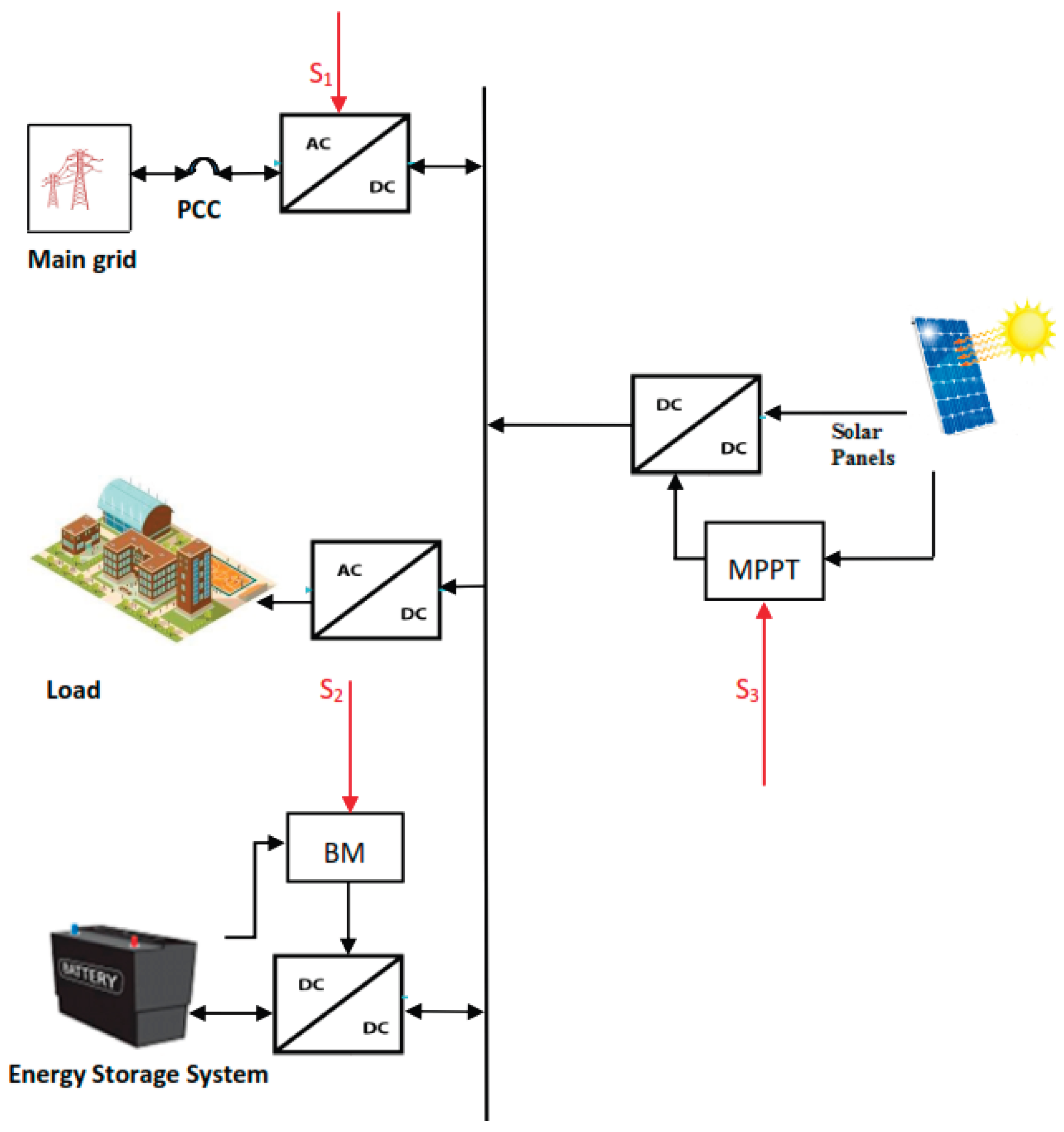
Figure 4.
EMS scheme.
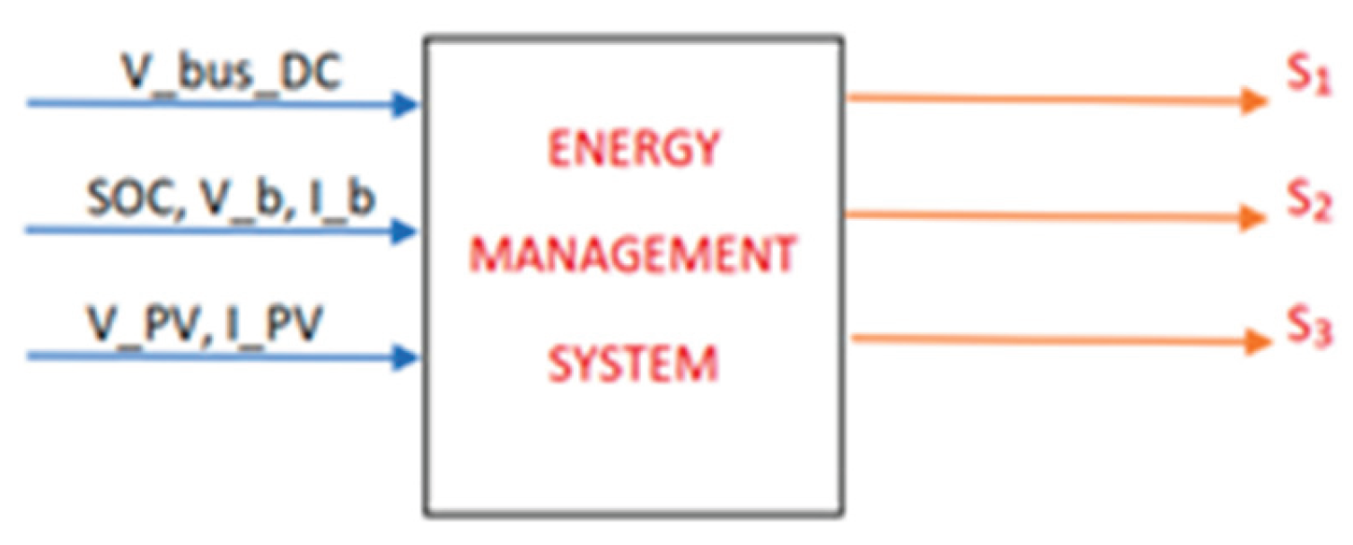
Figure 5.
Flowchart of the implemented methodology.
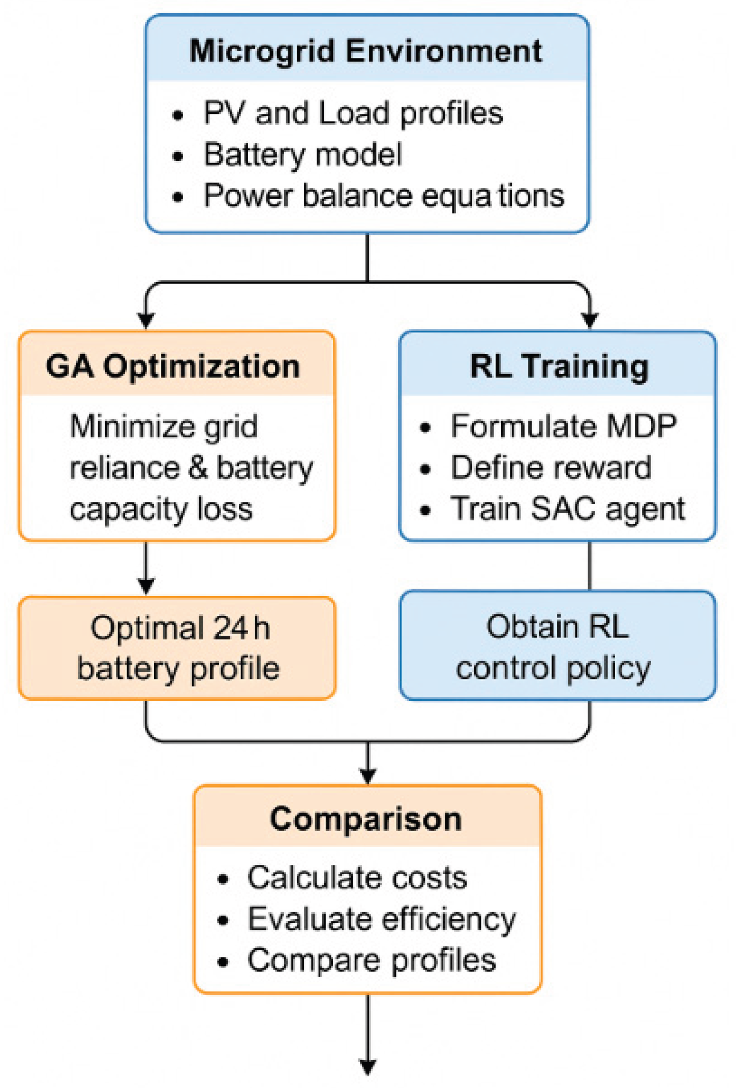
Figure 6.
8 PV power scenarios.
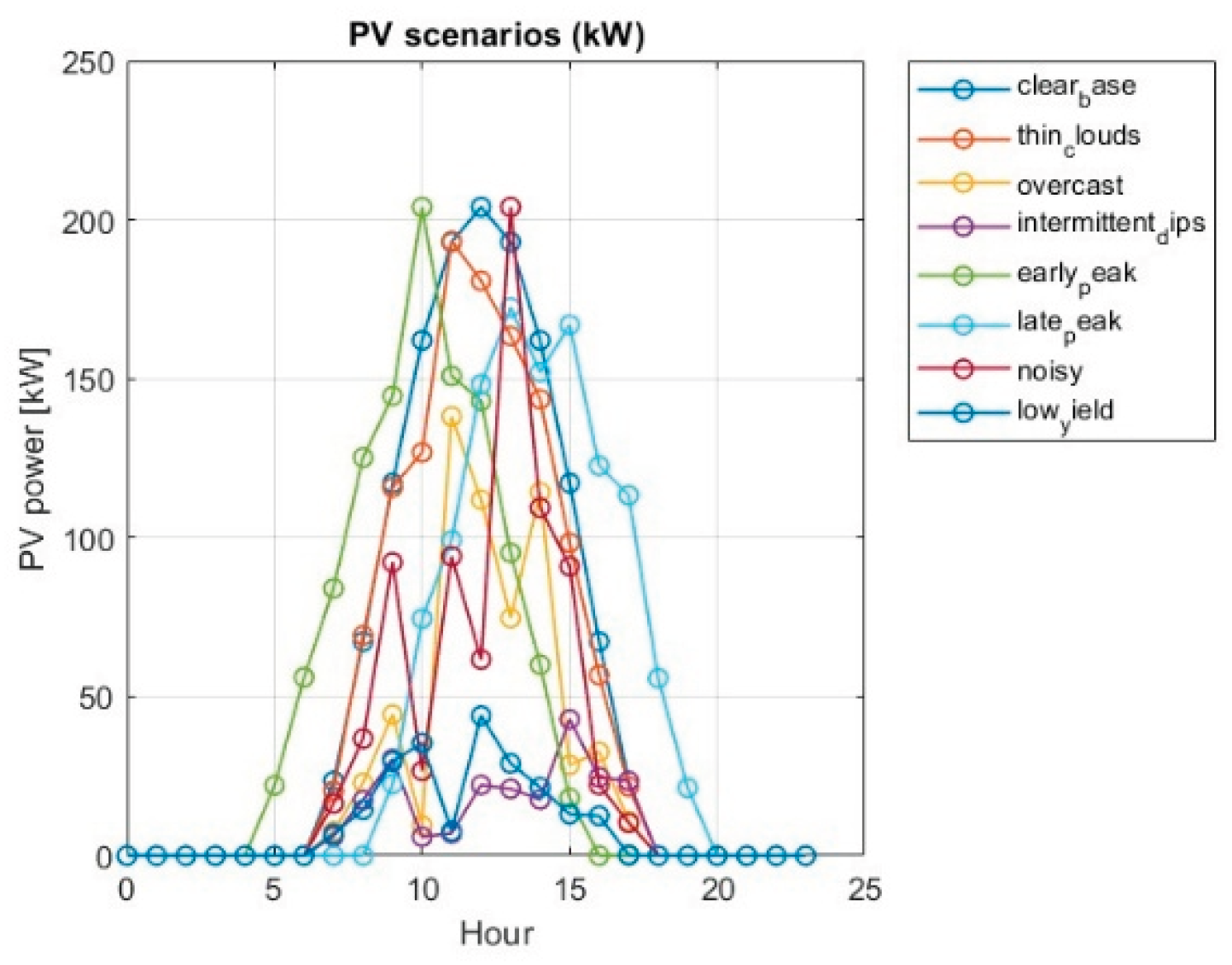
Figure 7.
8 Load scenarios.
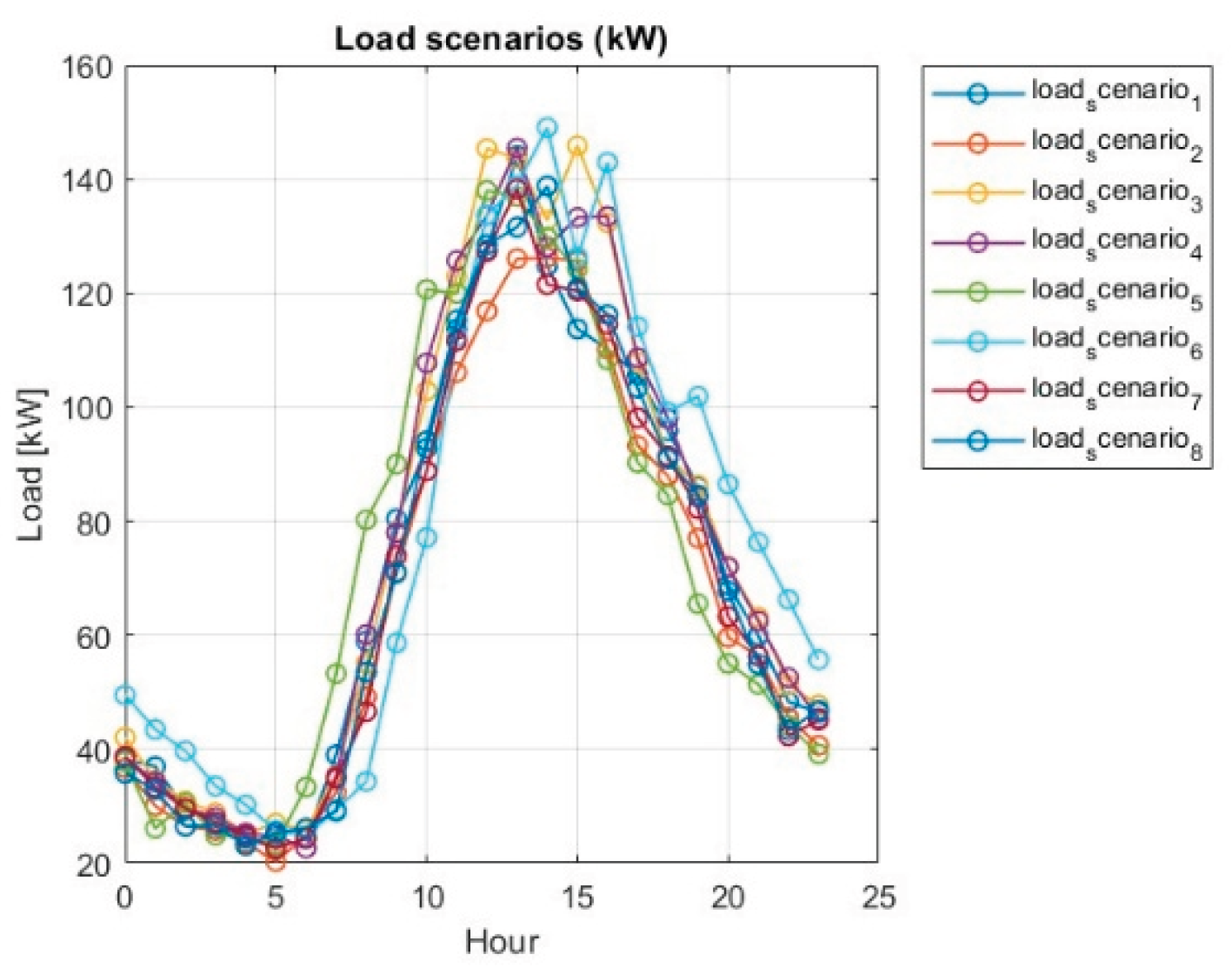
Figure 24.
Flowchart of the SAC agent.
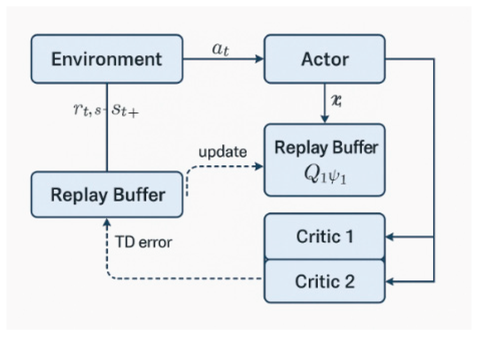
Figure 25.
Penalty breakdown graphics.
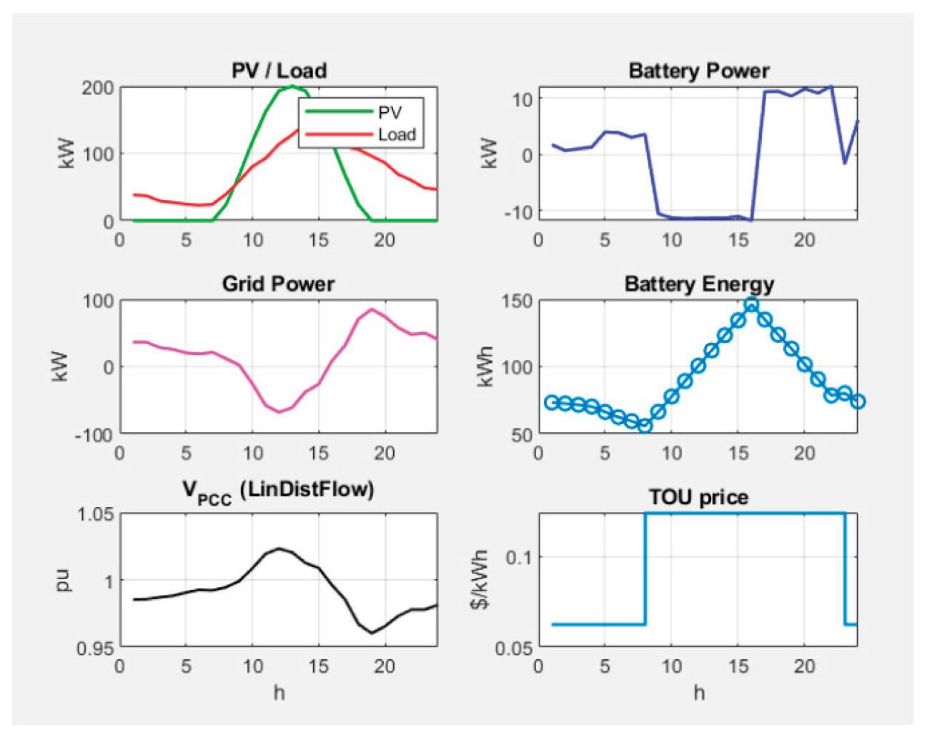
Figure 26.
Example of the Reward function for one scenario.
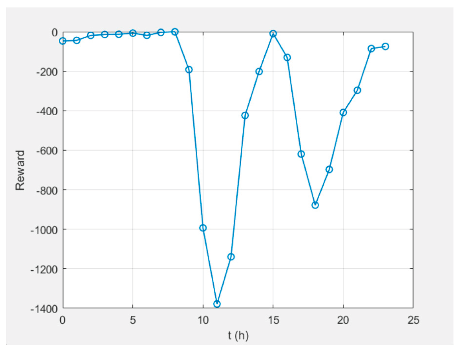
Figure 35.
Average reward across scenarios.
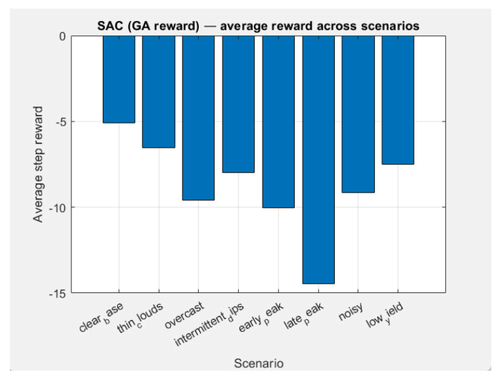
Figure 36.
RMSEPgrid for Scenario 1.
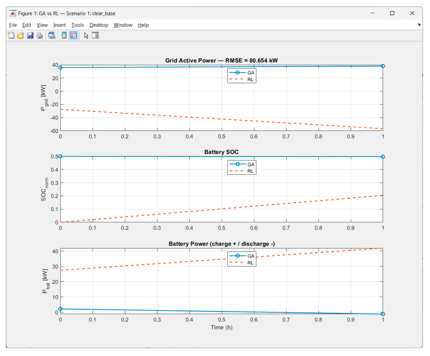
Figure 37.
RMSEPgrid for Scenario 4.
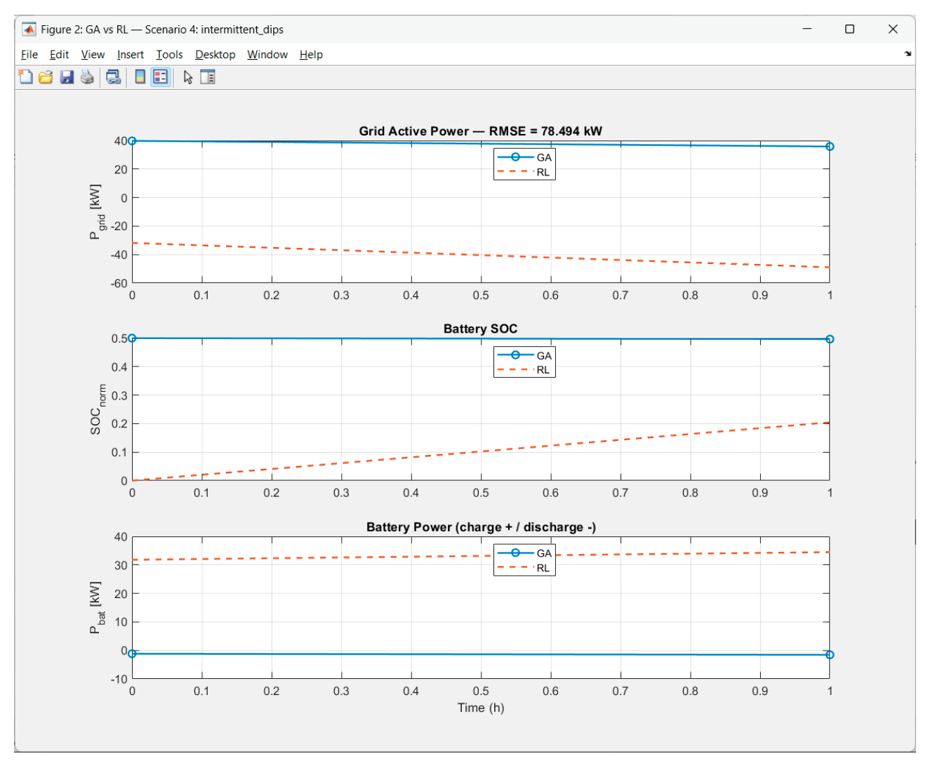
Figure 38.
RMSESOC for all scenarios.
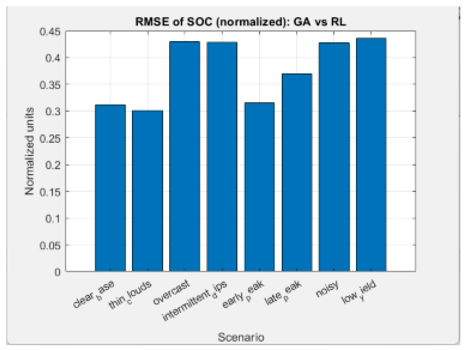
Figure 39.
RMSEPgrid for all scenarios.
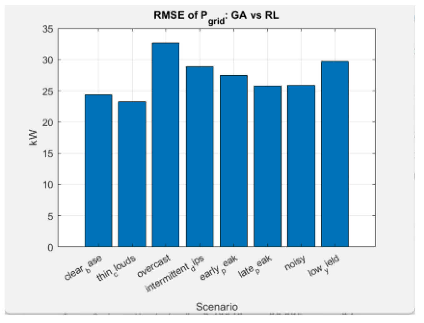
Table 1.
Table 1. Results from the GA-optimization, part 1.
| Scenario | Name | Pgrid_mean_kW | Egrid_pos_kWh | Egrid_neg_kWh | Battery_ throughput_kWh |
| 1 | "clear_base" | 16.22 | 688.77 | 299.49 | 127.40 |
| 2 | "thin_clouds" | 17.126 | 666.92 | 255.89 | 110.78 |
| 3 | "overcast" | 51.39 | 1233.4 | 0. | 126.81 |
| 4 | "intermittent_dips" | 66.202 | 1588.9 | 0. | 127.96 |
| 5 | "early_peak" | 26.223 | 849.3 | 219.95 | 118.29 |
| 6 | "late_peak" | 29.212 | 744.33 | 43.245 | 113.04 |
| 7 | "noisy" | 37.195 | 931.97 | 39.29 | 107.21 |
| 8 | "low_yield" | 61.376 | 1473. | 0. | 120.27 |
Table 2.
Results from the GA-optimization, part 2.
| Scenario | Name | Voltage_ frac_ outside | Voltage _max_abs_dV_pu | Voltage _std_pu | JGA | Energy _cost_USD |
| 1 | "clear_base" | 0. | 0.034277 | 0.017945 | 51066.2956 | 68.422 |
| 2 | "thin_clouds" | 0. | 0.030768 | 0.015615 | 42130.6795 | 66.062 |
| 3 | "overcast" | 0. | 0.035918 | 0.010297 | 79125.0423 | 131.72 |
| 4 | "intermittent_dips" | 0. | 0.046466 | 0.011876 | 124669.9913 | 174.68 |
| 5 | "early_peak" | 0. | 0.039037 | 0.017769 | 60999.7378 | 90.963 |
| 6 | "late_peak" | 0. | 0.027827 | 0.010297 | 36298.2641 | 69.749 |
| 7 | "noisy" | 0. | 0.033236 | 0.011507 | 6019.9 | 97.832 |
| 8 | "low_yield" | 0. | 0.043204 | 0.011098 | 12610. | 161.86 |
Table 3.
Main hyperparameters of the SAC-agent.
| Parameter | Description | Value |
| Learning rate (actor/critic) | Learning rate | 1×10⁻⁴ |
| Replay buffer size | Number of stored trials | 10⁵–10⁶ |
| Batch size | Mini-batch size | 256 |
| Discount factor (γ) | Discount factor | 0.99 |
| Entropy coefficient (α) | Research coefficient | Automatic tuning |
Table 4.
Results from the SAC-agent training in the 8 scenarios.
| Scenario index |
Scenario name | Average Reward | Final Reward |
| 1 | “Clear base” | -5.0879 | -4.1537 |
| 2 | “Thin clouds” | -6.5381 | -2.992 |
| 3 | “Overcast” | -9.5969 | -4.0345 |
| 4 | “Intermittent dips” | -7.9941 | -3.3311 |
| 5 | “Early peak” | -10.014 | -4.3793 |
| 6 | “Late peak” | -14.448 | -3.9954 |
| 7 | “Noisy” | -9.1458 | -24.857 |
| 8 | “Low yield” | -7.5129 | -8.7054 |
Table 5.
Root mean square errors results in the 8 scenarios.
| Scenario index |
Scenario name | RMSESOC | RMSEPgrid [kW] |
| 1 | “Clear base” | 0.3118 | 24.313 |
| 2 | “Thin clouds” | 0.30041 | 23.204 |
| 3 | “Overcast” | 0.42972 | 32.631 |
| 4 | “Intermittent dips” | 0.42842 | 28.825 |
| 5 | “Early peak” | 0.31498 | 27.481 |
| 6 | “Late peak” | 0.37009 | 25.746 |
| 7 | “Noisy” | 0.42808 | 25.866 |
| 8 | “Low yield” | 0.43595 | 29.686 |
Disclaimer/Publisher’s Note: The statements, opinions and data contained in all publications are solely those of the individual author(s) and contributor(s) and not of MDPI and/or the editor(s). MDPI and/or the editor(s) disclaim responsibility for any injury to people or property resulting from any ideas, methods, instructions or products referred to in the content. |
© 2025 by the authors. Licensee MDPI, Basel, Switzerland. This article is an open access article distributed under the terms and conditions of the Creative Commons Attribution (CC BY) license (http://creativecommons.org/licenses/by/4.0/).
Copyright: This open access article is published under a Creative Commons CC BY 4.0 license, which permit the free download, distribution, and reuse, provided that the author and preprint are cited in any reuse.


