
Submitted:
27 November 2025
Posted:
01 December 2025
You are already at the latest version
Abstract
Bipolar Polymer Membranes (BPMs) enable the creation of large, stable pH gradients by drivingwater dissociation (WD) at the cation/anion junction under reverse bias, a process central to electrodialysis, CO₂ capture, and emerging acid–alkaline water electrolysis. Yet, despite decades of study, the mechanism by which intense interfacial electric fields accelerate WD remains debated and is often modeled with ad hoc assumptions. Here, we outline key limitations of existing models of field-enhanced WD in BPMs and we present a power-dissipation model and its formalism that address them. In this new framework, we emphasize that minority ions from water autoprotolysis act as carriers that continuously dissipate field-supplied power in the hydrated nanometric junction. This dissipative input raises the local probability of heterolytic O–H bond cleavage and leads analytically to the dissociation rate’s quadratic dependence on the field. Without adjustable parameters, the model reproduces the required orders of magnitude for the enhancement ratio kd(E)/kd(0), where kd(E) is the field-enhanced water-dissociation rate constant and kd(0) its zero-field value, across typical BPM fields and yields a quadratic current–voltage junction law. A proof-of-principle measurement on a commercial Fumasep® FBM confirms the quadratic current–voltage trend, supporting a power dissipation field-driven WD and providing a concise, falsifiable baseline for future studies.
Keywords:
bipolar membranes
; new formalism
; water dissociation
; electric field
; autoprotolysis dissipated power
; nano metric junction
; water dissociation rate constant
; current-voltage curves
1. Introduction
Bipolar membranes (BPMs) are a unique class of polymer ion-exchange membranes (IEMs) [1], characterized by a laminated structure consisting of a cation-exchange membrane (CEM) on an anion-exchange membrane (AEM) [2]. This configuration enables BPMs to promote water dissociation (WD) at the junction of the two layers under reverse polarization [3], thereby sustaining large pH gradients across the membrane by generating hydronium (H₃O⁺) and hydroxide ions (OH⁻) [4].Originally developed for electrodialysis (ED) to produce acids and bases [5,6], BPMs Have Recently garnered substantial interest in advanced electrochemical applications [7], including brine valorization [8], CO₂ capture [9], fuel cells [10], and particularly in water electrolysis for hydrogen production [11,12].
Until now, the detailed mechanism of WD in BPMs—especially under intense interfacial electric fields—remained poorly understood. Under reverse bias, counterions migrate away from the CEM/AEM interface, creating a narrow space-charge region where an electric field exceeding 10⁸ V·m⁻¹ is established [13]. This field accelerates the dissociation of water molecules at the interface into H₃O⁺ and OH⁻ ions [8], which then migrate through the CEM and AEM, respectively. Using mass conservation, the flux of H₃O⁺ and OH⁻ out from the junction, cannot exceed the rate of their generation. Thus, the maximum WD current density in a BPM junction, was given by [5,14] :
where the parameters , , , , and are, respectively, the maximum WD current density in (A·m⁻²), the Faraday constant (96,485 C·mol⁻¹), the water dissociation rate constant in (s⁻¹), the water concentration at the interface in (mol·m⁻³) and the thickness of the BPM junction in (m). Eq. (1) explicitly assumes a reaction-limited WD with negligible recombination inside the junction, which is plausible for abrupt BPM junctions, where the transition region is a few nanometers [1],thus the nascent H₃O⁺ and OH⁻ are rapidly extracted into the CEM and AEM. In homogeneous BPMs with a uniform functional group distribution [15], the junction thickness does not exceed 1 nm [1,16]. In the absence of external field (E=0), the calculated water dissociation rate constant at 25 °C is = 2.5×10⁻⁵ s⁻¹ [17]. Assuming this nanometric junction is fully hydrated with pure water ( =55.5 mol·L⁻¹) [5], the predicted current density is only ~1.4 × 10⁻⁴ A·m⁻² [5]. However, experimentally observed BPM current densities can exceed 1000 A·m⁻² [5], implying an enhancement of by at least 7×10⁶ times the thermal value at 25 °C. This striking discrepancy is at the heart of a longstanding theoretical challenge.
Existing models—such as the Second Wien Effect (SWE) and catalytic protonation–deprotonation mechanisms—do not consistently explain this increase. Consequently, new theoretical frameworks are needed to predict and optimize BPM performance. In this context, we propose a power dissipation-based model in which WD is driven by field-supplied power to autoprotolysis ions in water. The model establishes a quadratic dependence of on the field , which yields to a quadratic current–voltage junction law.
This manuscript is organized as follows. Section 2 reviews the state-of-the-art theoretical models of water dissociation in bipolar membranes. Section 3 details the theoretical development of our power dissipation model, its mathematical relations and associated theoretical results, while Section 4 presents the experimental methods. Section 5 provides results and discussion, and Section 6 the conclusion.
2. State-of-the-Art Models for Water Dissociation (WD) Enhancement in BPMs Junctions
Understanding the sharp increase in the WD rate in BPMs has been a long-standing challenge. Several theoretical models have been proposed, two of which dominate current discussions: the SWE and the catalytic protonation–deprotonation mechanism involving membrane functional groups. Despite their respective limitations, these models are widely used in BPM modeling [3,18,19,20]. We briefly summarize their scope and limitations, together with alternative approaches.
2.1. Second Wien Effect (SWE)
The Second Wien Effect (SWE) was the first mechanism proposed to account for the increase in WD under an electric field [21,22]. Based on Onsager’s theory [23], it describes how a strong electric field enhances the dissociation of ion pairs in weak electrolytes. For high electric fields (E > 10⁸ V·m⁻¹), the ratio / can be determined by [23].
where , is the field strength (V·m⁻¹), is the relative permittivity, and is the temperature in (K). While pure water is often treated as a weak electrolyte due to its low ionic concentration (~10⁻⁷ mol·L⁻¹), applying SWE to water has serious limitations [24,25,26]. First, Onsager’s theory assumes pre-existingion pairs, not neutral water molecules [27,28]. Second, water’s high dielectric constant (~80 at 25 °C) makes the formation of stable ion pairs unlikely [22,23]. Moreover, the SWE-predicted dissociation rates remain far too low to explain the experimental results obtained using BPM. According to Strathmann [5], it can only match observed values if is reduced below 10. Krol [14] discussed the role of relative permittivity in SWE, highlighting the difficulty of determining and its complexity when considering it as field-dependent, especially under high fields where can drop from 78 to 16 for E = 2×10⁹ V·m⁻¹ [14]. Empirical formulas support this trend [29,30].
However, this points out a conceptual issue: may decrease because of an increase in ion concentration, as supported by the Hückel’s theory [31], which could mean the field-induced dissociation itself causes the drop in , reversing the assumed causality. Furthermore, the SWE’s exponential sensitivity to E results in numerical instability when varying with E : applying Eq. (1) and (2) gives 1210 A·m⁻² at 10⁹ V·m⁻¹, but an unrealistic 10⁸ A·m⁻² at 2×10⁹ V·m⁻¹. Also, water’s may drastically decrease in confined environments [32] even without an electric field—yet inserting such values into SWE remains problematic.
2.2. Catalytic Protonation–Deprotonation Mechanism
The second mechanism, introduced by Simons [33,34], proposes that WD is catalyzed by membrane functional groups—namely, BH⁺ in the AEM and A⁻ in the CEM—through the following reactions:
B + H2O ⇌ BH+ + OH- ,
BH+ + H2O ⇌ B + H3O+,
A + H2O⇌AH + OH-
AH + H2O ⇌ A- + H3O+.
However, this mechanism yields dissociation kinetics that are too slow [28]. This low kinetics prediction led to the development of the Chemical Reaction Model (CRM) [35,36,37], where the electric field is assumed to accelerate pro tonation reactions between water and fixed charges. Relying on statistical arguments about the field-induced alignment of water molecules and catalytic sites [28,38], the water dissociation enhancement based on the Chemical Reaction Model trough its rate constant given as :
where is the field-enhanced WD rate constant due to protonation-deprotonation reactions of water molecules with fixed charges, is a fitting parameter homogenous to a length, F is the Faraday constant (96,485 C·mol⁻¹), E is the applied field (V·m⁻¹), R the universal gas constant (8.314 J·mol⁻¹· K⁻¹) and is the rate constant when no field is applied given by an Arrhenius expression [28,38]:
where A is the pre-exponential factor and EA is the activation energy., R is the gas constant and T is the temperature.
According to CRM model, the maximum WD current density J in the BPM junction, depends on the concentration of catalytic fixed groups , and is given by:
where all the parameters are defined in the above corresponding relations. This CRM model formulation relies on multiple poorly defined parameters that are difficult to determine independently: The concentration of the catalytic groups, the pre-exponential factor A, and the constant α. Thus, making difficult an accurately modeling ion transport in BPMs.
Recent literature [18,38] often identifies the parameter with the Bjerrum length , over which a dipole is dissociated into its respective ions in a medium, using an SWE approximation at low fields. However, the SWE exponential formula with overestimate the increase in leading to unphysical divergences [18].
2.3. Alternative Models
Martinez and Farrell [13] used quantum chemical simulations to evaluate under strong electric fields. Their results resemble SWE predictions and rely also on a reduction in . Saitta et al. [39] reported water dissociation thresholds of 3.5×10⁹ V·m⁻¹ and up to 15–20% dissociation at 10¹⁰ V·m⁻¹ using molecular dynamics, but such field strengths far exceed those in BPMs. Hurwitz and Dibiani [25,40] attempted to propose an electrochemical model, where the WD is seen as a redox-like process involving H⁺ and OH⁻ ions by exploiting its heterolytic nature [25,40], thereby justifying Tafel or Butler–Volmer treatments [28]. However, such an analogy lacks a solid basis in BPMs, where no electron Transfer occurs, and WD is better described as a chemical reaction, not governed by an electrochemical reaction involving electron transfer at electronic/electrolyte interface, in the strict sense. Additional proposals invoke semiconductor p– n junction analogies [41,42] or ion solvation kinetics [43], but still fail to recover the orders of magnitude required for /quantitatively. Recent transport models even omit a specific WD mechanism and assume “sufficiently fast” dissociation [44].
Overall, despite clear evidence that strong fields enhance WD, existing models do not consistently explain this increase. Motivated by the quantitative mismatch summarized above, we propose a power dissipation-based framework in which WD is driven by dissipated field-supplied power to autoprotolysis ions. The resulting picture establishes a quadratic dependence of on the field and provides a compact route to device-level predictions.
3. Theoretical
3.1. Power Dissipation Model for Electric-Field-Driven WD
3.1.1. Framework and Working Hypothesis
In aqueous electrolytes, field-driven transport of ions follows the well-known drift regime [45]. Under the influence of an electric field E, an ion of charge q experiences an electric force proportional to the field E:
which is opposed by viscous friction :
where f is the friction coefficient and v is the ion velocity. Within an extremely short time, these forces balance:
so the ion moves at a constant drift velocity vd proportional to E:
where µ is the ionic mobility in (m²·V⁻¹·s⁻¹). Although no kinetic energy accumulates in this steady state, the field continuously injects energy that is entirely dissipated by viscous friction at a rate corresponding to field-supplied power per ion P in (J·s⁻¹), given by
Liquid water always contains minority ions H₃O⁺ and OH⁻ at very low concentration 10⁻⁷ mol·L⁻¹ at 25 °C, due to autoprotolysis :
with an equilibrium constant at 25 °C. When an electric field is applied to liquid water, these minority ions are the only species that undergo field-directed motion and dissipate power, whereas neutral H₂O molecules may merely reorient their dipoles. For BPM-relevant strong fields (E≳10⁸ V·m⁻¹), the per-ion dissipated power of H₃O⁺ and OH⁻ is non-negligible and potentially chemically relevant at the molecular scale. Order-of-magnitude estimates support this plausibility:
At 25 °C, = 3.62 ×10⁻⁷ m²·V⁻¹·s⁻¹ and = 2.05 ×10⁻⁷ m²·V⁻¹·s⁻¹ [46].
For a typical BPM-field E =10⁸ V·m⁻¹, with q = 1.6 ×10⁻¹⁹ C for both ions H₃O⁺ and OH⁻, the drift powers, using Eq. (14) are:
≈ 5.79 × 10⁻¹⁰ J·s⁻¹ and ≈ 3.28 × 10⁻¹⁰ J·s⁻¹.
The molar Gibbs free energy of dissociation (forward reaction in Eq. 15) is obtained from the equilibrium constant as:
At 25 °C, = 79.9 kJ·mol⁻¹, meaning that the theoretical energy required to dissociate one mol of water is 79,9 kJ [47]. The per-molecule dissociation threshold energy (in J) required to dissociate one water molecule is obtained from the molar Gibbs free energy of dissociation by:
where NA = 6.022×10²³ mol⁻¹ is Avogadro’s number. At 25 °C, ≈ 1.33 ×10⁻¹⁹ J.
Thus, under E =10⁸ V·m⁻¹ each single H₃O⁺ and OH⁻ ion can, in theory, dissipate enough energy each second to induce:
= 4.35 ×10⁹ and = 2.46 ×10⁹ potential dissociation events per second, respectively.
In the specific context of BPMs under reverse bias, once the junction is depleted of mobile counter-ions, the residual current is carried by the minority autoprotolysis ions H₃O⁺ and OH⁻[5,14]. Because enhanced water dissociation is observed after this minority-carrier regime is established, it is natural to consider WD as a consequence of that pre-existing drift—the real process through which the field supplies power to the system.
Scaling up to a fully hydrated BPM with a surface area A = 1 cm² and a junction δ = 1 nm, the volume of the junction is Vⱼ =10⁻¹³ m³. With concentrations of liquid water in the junction and the minority autoprotolysis ions of = 55.5 mol·L⁻¹ and cᵢₒₙₛ = 10⁻⁷ mol·L⁻¹, respectively. The total power dissipated by all the ions H₃O⁺ and OH⁻ present in the junction’s volume Vⱼ can be expressed as:
where in (m⁻³) is the volumetric density of ions H₃O⁺ and OH⁻, given by :
where is the concentrations of ions. The are equal (i.e. , since they have the same concentration. The volume Vⱼ contains 3.3 ×10¹⁵ water molecules and 6.022 ×10⁶ H₃O⁺ and OH⁻ ions each. The total dissipated power for E = 10⁸ V·m⁻¹ is ≈ 5.46 ×10⁻³ J·s⁻¹. The corresponding number of potential dissociations events per second is 4.1 ×10¹⁶, meaning that the entire water content of the junction could, in theory, dissociate in less than one second. Furthermore, given the thermal conductivity of water (κ ≈ 6 × 10⁻³ J·s⁻¹·cm⁻¹·K⁻¹) and the nanometric thickness of the junction (δ = 1 nm), a simple steady-state heat-flux estimate using the expression [48]:
gives a temperature rise ΔT ≈ 5×10⁻⁸ K, showing that Joule heating is negligible at the junction scale, and the system can be treated as effectively isothermal under the conditions considered. In this isothermal limit, the power dissipated by the drift of autoprotolysis ions corresponds, in the sense of non-equilibrium thermodynamics, to the internal entropy production according to [49]:
Thus, the dissipated power in the nanometric junction is interpreted as local entropy production, which can drive microscopic molecular rearrangements and provides a physically consistent basis for relating dissipation to field-assisted water dissociation.
Building on the estimates above, our working hypothesis is that the dissipated power of the drifting autoprotolysis ions (H₃O⁺, OH⁻) under strong electric fields is more than sufficient to drive new water-dissociation events per second. Thus, the sudden increase of the WD rate observed in BPMs at high electric field is an indirect ion-mediated consequence of power dissipation rather than a direct field action on neutral water molecules. Therefore, in the BPM junction the intense electric field raises the effective probability of dissociation, by amplifying the frequency of activation attempts powered by drift dissipation above the dissociation energy Ed. Accordingly, we postulate that the WD rate constant is proportional to the ratio of the total dissipated power over : ∝.
3.1.1. Analytical Formulation of kd(E)
We interpret the WD rate constant as a frequency of energy delivery relative to the activation barrier. Let the power density w ( J·s⁻¹·m⁻³), deposited by all field-driven ions H₃O⁺ and OH⁻ be
whereand are respectively the volumetric density of H₃O⁺ and OH⁻, and are, respectively, the dissipated power by H₃O⁺ and OH⁻. Since the concentrations of H₃O⁺ and OH⁻ in pure water are equal (i.e. = 10⁻⁷ mol·L⁻¹), their volumetric density is also equal (). Thus,
Dividing by the threshold dissociation energy per event gives a volumetric event rate (s⁻¹· m⁻³):
The per-molecule (pseudo–first order) rate constant in (s⁻¹) is then obtained by normalizing by the number density of water molecules:
Since
and replacing and by their respective formulas, i.e.
And
we obtain the final expression of (E), as :
where,
: Dissociation rate constant of water molecules as a function of the field E in (s⁻¹),
cᵢₒₙₛ: Concentration of H₃O⁺ and OH⁻ ions in water (10⁻⁷ mol·L⁻¹ at 25 °C),
: Concentration of free liquid water (55.5 mol·L⁻¹ at 25 °C),
q: Absolute electric charge of H₃O⁺ and OH⁻ ions (q = 1.6 ×10⁻¹⁹ C),
: Ionic mobility of the hydronium ion H₃O⁺ (3.62 ×10⁻⁷ m²·V⁻¹·s⁻¹ at 25 °C),
: Ionic mobility of the hydroxide ion OH⁻ (2.05 ×10⁻⁷ m²·V⁻¹·s⁻¹ at 25 °C),
E: The electric field in the BPM junction in (V·m⁻¹),
: Threshold dissociation energy per water molecule in (J), ( = 1.33 ×10⁻¹⁹ J at 25 °C).
This formulation reveals ’s simple quadratic dependence on electric field E, representing a significant departure from previously proposed exponential models. It provides a clear analytical link between physicochemical parameters—elementary charge, ion mobility, dissociation energy, and molar concentrations—and the dissociation rate, without relying on empirical constants or catalytic assumptions. This analytical form enables a direct estimation of the dissociation rate as a function of the electric field E applied at the BPM junction.
We note that mobilities of H₃O⁺ and OH⁻ in water are obtained from [50]:
where is the limiting molar conductivity at infinite dilution in (S·m²·mol⁻¹) and F is the Faraday constant (96,485 C·mol⁻¹). It was shown that is independent of the field strength [51], so are the mobilities. In addition, studies reported a negligible influence of high electric fields on the viscosity η of solvents [52,53]; as per Stokes–Einstein relation µ ∝ 1/η [46], the effect is also negligible on .
Furthermore, Eq. (29) carries an implicit temperature dependence (T) via three parameters: µ, which increases with T via η [54], and cᵢₒₙₛ and , which also increase with T via the Nernst relation (Eq. 16) [55].Overall, the model relies solely on measurable, field-independent quantities at constant temperature. By substituting standard values at 25 °C into Eq. (29), we obtain the following simplified expression for the water dissociation rate:
This equation will be used for comparison benchmarks with SWE at 25 °C in section 3.2.1.
3.1.2. Junction J-V Relation Derived from
Under reverse bias, the current in a BPM primarily results from the migration of ions generated by water dissociation at the junction, which is captured by Eq. (1). Let Uⱼ denote the junction voltage drop across the active region of thickness δ. Assuming a quasi-uniform field in the junction:
By replacing E of Eq. (29) with its Eq. (32) expression and inserting Eq. (29) for (E) into Eq. (1), we obtain
where,
is the ratio of the effective water concentration in the junction to the concentration of free liquid water. The parameter f is a dimensionless factor representing the water volume fraction in the BPM junction [56,57,58], which varies from 0 (no water) to 1 (fully hydrated junction). Let
then Eq. (33) simplifies to :
where K is in (mA·cm⁻²·V⁻²), if J and Uⱼ are in (mA·cm⁻²) and volts (V), respectively.
Assuming a homogeneous BPM with a nanometric junction δ=1 nm, fully hydrated (f = 1), and standard physical constants at 25 °C, Eq. (36) gives
We emphasize that Eq. (36) is a junction-level law; in experiments, what is controlled is the external cell voltage . The experimental determination of Uⱼ from is described in the experimental section.
3.2. Theoretical Results
3.2.1. Enhancement and Comparison with SWE
Figure 1 shows the resulting curve (E) at 25 °C from Eq. (31), at a 0–100 s⁻¹ y-axis scale. Note that this scale compresses the low-field region: although Eq. (31) yields a strictly quadratic onset from E=0, (E) remains < 1 s−1 up to E ≈ 2.8×10⁷ V·m⁻¹, so the curve appears nearly flat at this scale (a zoom reveals the monotonic rise).
The profile closely resembles typical BPM J–V behavior where an initial low-conductivity region is followed by a sharp increase beyond a threshold. The crossover where = occurs at E* ≈1.43×10⁵ V·m⁻¹. For a nanometric BPM junction (δ=1 nm), this field corresponds to a voltage of 0.14 mV. At fields below E*, the overall dissociation is governed by the thermal constant . From E* up to ∼2.8×10⁷ V·m⁻¹ (Uⱼ ≈28 mV for δ=1 nm), (E) exceeds but remains < 1 s−1; rates are still weak, indicating a non-activated regime where the field is insufficient to trigger significant dissociation. A sharp transition emerges above 10⁸ V·m⁻¹, corresponding to voltages Uⱼ ≳0.1 V in the nanometric junction, marking the onset of an activated regime where the field supplies enough power to accelerate dissociation. To quantify this transition, values of (E) and the amplification ratio across the activated field range are reported in Table 1:
These values show consistent increases in , from ~ 5×10⁵ to ~2×1
These values show consistent increases in , from ~ 5×10⁵ to ~2×10⁸, over the field range 10⁸–2×10⁹ V·m⁻¹, aligning with experimental requirements for sustaining current densities of 10 to several hundred mA/cm². The quadratic form thus captures the field activation effect realistically: the progression is rapid yet stable, avoiding numerical divergence and remaining compatible with electrochemical integration through Eq. (1).
To further contextualize our model, we compare it with the SWE model. Table 2 presents the ratios for each model at two representative fields (10⁸ and 2×10⁹ V·m⁻¹), corresponding to 0.1 V and 2 V across a 1 nm-thick BPM junction. For SWE model, both the constant permittivity ( =78) and field-dependent permittivity cases are considered (78 to 16 for E = 10⁸ to 2×10⁹ V·m⁻¹). Two more scenarios with fixed (10 and 5) are considered to account for possible nanoconfinement effects.
The results highlight the fundamental disparities between the models. In SWE model, small field variations cause drastic shifts in . At E =10⁸ V·m⁻¹, SWE remains weak across both choices, whereas the quadratic law already yields ~ 5×10⁵. The SWE model with constant shows a limited increase (< 5×10⁴) at 2×10⁹ V·m⁻¹, which is insufficient for supporting BPM current densities. Its variable- version improves predictions but introduces instability, with a sharp divergence at 2×10⁹ V·m⁻¹. Nanoconfinement effects does not alter the qualitative conclusion that SWE either underestimates activation at 10⁸ V·m⁻¹ or becomes unstable at higher fields. By contrast, our quadratic model exhibits a large yet controlled amplification, without runaway divergence over the same field window E ∈ [10⁸–2×10⁹] V·m⁻¹, providing a robust basis for BPM-relevant modeling.
3.2.2. Theoretical J-V Curve of a Nanometric BPM Junction Fully Hydrated
Figure 2 shows the resulting J–Uⱼ curve of a BPM nanometric junction (δ =1 nm) fully hydrated (f =1), at 25 °C from Eq.(37).
The curve features a smooth, continuous increase in current, with no apparent threshold. At low voltages, the current remains low but non-zero, reflecting a gradual activation of dissociation. As the voltage increases, the field intensifies, and the current increases quadratically. This curve defines a theoretical upper bound (homogeneous, fully hydrated 1 nm junction; uniform field; no interfacial resistance). It thus serves as a universal benchmark for interpreting experiments and diagnosing losses (partial hydration f < 1, thicker effective junction δ > 1nm, ohmic drops and electrode overpotentials), which are analyzed in Section 4 and discussed later.It should be noted that Uⱼ = 1 V already gives a theoretical current of J = 660 mA·cm⁻². At Uⱼ = 1.75 V, we approach 2 A·cm⁻², which corresponds to the typical current of PEM electrolyzers. It can also be noted that the current density of J = 100 mA·cm⁻² corresponds to a voltage of Uⱼ = 0.38 V, i.e. a field E = 3.8×10⁸ V·m⁻¹, for a 1 nm BPM junction. The corresponding ratio obtained by our model is 7×10⁶, a value fully consistent with BPM observations from Section 1. This agreement further supports the predictive strength and physical consistency of our quadratic model.
4. Materials and Experimental Methods
4.1. Membrane and Electrodes
A commercial bipolar membrane (Fumasep® FBM, acquired from FuelCell Store) was cut to samples of 1.0 cm² active area. The acidic-side working electrode was Pt foil (1.0 cm²), and the alkaline-side working electrode was Ni foam (1.0 cm²), both obtained from Sigma Aldrich (Oakville, Canada). They were cleaned using acetone, deionized water, alcohol and deionized water before use. These electrodes are commonly used for BPM water electrolysis characterisation [11,59].
4.2. Electrolytes, Cell Type and Components
Experiments were performed in an H-cell, (Stony Lab, Nesconset, New York USA) with two liquid compartments separated by the BPM. The acidic compartment contained H₂SO₄ (pH=0) 0.5 M and the alkaline compartment contained NaOH 1.0 M (pH=14). The inter-electrode spacing was 10 cm (non-zero-gap); the electrode–membrane distance was 5 cm on each side. Unless stated otherwise, measurements were conducted at 25 °C. We emphasize that this is an electrolysis configuration (acid|BPM|alkali), not an electrodialysis stack.
4.3. Electrochemical Instrumentation and Measurement Protocols
Linear sweep voltammetry (LSV) was performed in a two-electrode configuration on the full BPM cell, using a Solartron 1287A potentiostat/galvanostat (Scribner, North Carolina, USA). The cell voltage was swept at 5 mV·s⁻¹. Electrochemical impedance spectroscopy (EIS) was performed with a VersaSTAT 4A (Ametek, Oak Ridge, Tennessee ,USA), using a small-signal sinusoidal perturbation (10 mVᵣₘₛ) over a log-spaced frequency sweep from 1 MHz down to 0.1 Hz. For the two-compartment BPM cell, global series resistance was obtained from the high-frequency real-axis intercept of the Nyquist plot; values are reported in Ω·cm² after normalization by 1.0 cm² geometric area. Data and extraction details are provided in Section 5. LSVs were collected as raw curves and, when specified, as -corrected curves using the obtained from EIS.
4.4. Three-Electrode Configuration Characterization of the Hydrogen Evolution Reaction (HER) and of the Oxygen Evolution Reaction (OER)
To quantify electrode kinetics independently of the membrane cell, we performed three-electrode configuration measurements for the hydrogen evolution reaction (HER) and for the oxygen evolution reaction (OER) in their respective electrolytes. In this study the hydrogen gas pressure is 1 atmosphere (PH2 = PO2= 1 atm). The following half-reactions are considered in their respective compartment with their equilibrium potentials referenced to the Reversible Hydrogen Electrode (RHE) which potentials at standards conditions are, respectively, =0 V vs RHE for the HER at pH=0, and = 1.23 V vs RHE for the OER at pH=14 [47]:
In the acidic compartment the following Hydrogen Evolution Reaction (HER) occurs:
The dependence of the equilibrium potential of the reaction with the pH is:
Here, pH = 0, PH2 = 1 and T = 298 K which are standards conditions. Then:
In the alkaline compartment, the following Oxygen Evolution Reaction (OER) occurs
The dependence of the equilibrium potential of the reaction with the pH is :
In this compartment, pH = 14
For HER in 0.5 M H₂SO₄, the reference electrode was Hg/HgSO₄; for OER in 1.0 M NaOH, the reference electrode was Hg/HgO. All potentials were converted to RHE using fixed offsets (Hg/HgSO₄ (sat.) = 0.64 V vs RHE; Hg/HgO = 0.098 V vs RHE). The Solartron 1287A applied 100% iR compensation in these three-electrode tests (note that this R is not the same as the two-compartment BPM cell ). Overpotentials were computed as:
where and are, respectively, the applied potential to the electrode of the hydrogen evolution reaction in the acidic compartment and of the Oxygen Evolution Reaction in the alkaline compartment, during the tests. Each of the potential vs current plots displays a Tafel behaviour in a certain range of potential according to:
for the HER, and
for the OER.
The respective HER and OER Tafel slopes and and their corresponding exchange current densities and were obtained by linear fits of the above Tafel forms applied in the appropriate overpotential ranges where E-log J is quasi-linear. Precisely, we used:
-HER: low overvoltage window ∈ [-65,–45] mV (cathodic currents, after taking in account the value of the reference electrodes and iR-compensation).
-OER: window ∈ [+0.20,+0.35] V (controlled by activation regime, iR-compensated).
The numerical values of the extracted Tafel slopes and exchange current densities values are reported in Section 5, together with the corresponding polarization and Tafel plots (including the fitted windows).
4.5. BPM’s Junction-Voltage Accounting
For comparison to the theoretical junction law, we computed the junction drop Uⱼ from the external cell bias by removing equilibrium, series resistance and overpotentials contributions [57,58]:
where is the reversible equilibrium voltage of the cell :
Since V vs RHE and V vs RHE, then V vs RHE. The LSV-derived current densities were then compared to the model prediction Eq. (37). All fits and goodness-of-fit metrics are presented in Section 5.
5. Results and Discussion
Figure 3 shows the raw J vs curve of Fumasep® FBM obtained from LSV (two-compartment FBM cell, ΔpH=14). A measurable current appears near 1.36 V (sub- mA·cm⁻²), while the 1 mA·cm⁻² onset occurs at ≈ 1.42 V. The curve exhibits 3 salient regions: First, a linear ohmic-like rise between 1.36–1.54 V, followed by quasi-stationary plateau between 1.55 and 1.62 with an average limiting current density Jlim ≈ 2.19 mA·cm⁻², then a transition into an over-limiting regime beyond ∼1.62 V, where the current leaves the shelf and increases rapidly. This morphology is the canonical BPM signature at low current densities [3,44]: an initial rise, a limiting shelf associated with internal depletion in the ion-exchange layers, then take-off as the junction field grows and water dissociation (WD) becomes dominant.
Importantly, a linear fit over 1.36–1.54 V (Figure 4.a) is excellent with slope 10.73 mA·cm⁻²·V⁻¹ and , indicating an ohmic behavior governed by co-ions transport. Yet, when we re-plot the same data against (Figure 5), a quadratic form fits equally well on that narrow span. This apparent paradox suggests that the low-bias current is composite: a nascent WD channel already contributes below 1 mA cm⁻², as emphasized by recent literature [44], while a residual co-ions transport path (imperfect permselectivity through the ion-exchange layers) adds an ohmic-like component. By contrast, the quasi-plateau 1.55–1.62 V (with Jlim ≈ 2.19 mA·cm⁻²) is not captured by a pure quadratic law (Figure 5) and marks the limiting-current shelf typical of BPMs at low current densities. For completeness, a quadratic fit restricted to 1.36–1.54 V with (K=21.94 mA·cm⁻²·V⁻², ) is provided in (Figure 4.b).
Subtracting only the equilibrium reversible voltage ( ≃ ) yields already an excellent quadratic fit, with a prefactor K ≃ 21.25 mA·cm⁻²·V⁻², as shown in Figure 5. This supports our quadratic model and means that the cell current is mainly dominated by WD. The low prefactor compared to the theoretical K=660 reflects the fact that bulk ohmic loss and electrode overpotentials still remain in the trace. This supports the importance to make the ohmic loss and overvoltage correction, i.e. Eq. (48). Figure 6.a) shows the Nyquist plot obtained from the Electrochemical Impedance Spectroscopy (EIS) measurement. The area-normalized series resistance is extracted from the high-frequency real-axis intercept: = 20.19 Ω·cm². Figure 6.b) shows the corresponding iRs-corrected J vs Ecell curve.
Independent three-electrode HER & OER polarization curves, each with its own iR-correction (not the FBM-cell ), are shown in Figure 7.a) and Figure 7.b), respectively. These datasets supply and used in the junction mapping.
Independent three-electrode characterizations provided a Tafel slope of -29.66 mV·dec⁻¹ and an exchange current density of 9.2 ×10⁻⁴ A·cm⁻² for HER on Pt (Figure 7.c). While for OER on Ni foam, a Tafel slope of 41.92 mV·dec⁻¹ and an exchange current density of 6.11 ×10⁻¹⁰ A·cm⁻² were obtained (Figure 7.d). These values are consistent with literature values for the respective HER and OER on these materials [60,61]. These values are used for the overpotential corrections in the full junction mapping which results are shown in Figure 8.
After full junction mapping using Eq.(48), the obtained J vs Uⱼ curve of the junction voltage collapse onto a robust quadratic law, with a much larger prefactor K ≃ 505.46 mA·cm⁻²·V⁻², as shown in Figure 8. We notice that in a narrow window Uⱼ ∈[0,0.07] V, the current remains nearly constant at J ≈ 2.2 mA·cm⁻², in excellent agreement with the limiting current measured on the raw LSV Jlim ≈2.19 mA·cm⁻².This flat shoulder reflects the transport-limited baseline that precedes strong field-assisted water dissociation (WD) in BPMs; it does not contradict the junction quadratic law. Subtracting this constant baseline would force the curve through the origin and numerically reduce the zero-intercept prefactor K (a generic effect of vertical offsets in least-squares), but adds no physical information; we therefore report only the full-mapping result in Figure 8 and interpret the small offset as the limiting baseline with minor reconstruction offsets expected at very low junction field.
The prefactor for Fumasep® FBM, K ≃ 505.46 mA·cm⁻²·V⁻² is ~76.6% of the ideal K = 660 mA·cm⁻²·V⁻² estimated for a 1 nm, fully hydrated junction (§3.1.3). Since the Fumasep® FBM is homogenous [62], a δ ≈1 nm active region is plausible (Section 1). Hence, the observed prefactor gap can be reasonably attributed to the water volume fraction f , as reflected in Eq. (35). Beyond hydration, the gap can also be explained by a slight deviation of the effective junction thickness from the 1 nm benchmark (e.g., nm, or conversely < 1 nm) or a dissipation efficiency α capturing non-productive channels, without affecting the quadratic law. Overall, the FBM junction exhibit a high-quality quadratic dependence of J on Uⱼ (≈0.99), with a high prefactor K after full junction mapping. These results provide a proof-of-principle of the quadratic (E) dependence anticipated by our power-dissipation model.
The above experimental results clearly indicate that our proposed model provides a novel power dissipation framework for interpreting WD enhancement under strong electric fields in BPMs with nanometric junctions. The central premise is that the dissipated power of drifting autoprotolysis ions H₃O⁺ and OH⁻ under field, raises the propensity for heterolytic O–H bond cleavage. Thus, these rare ions act as indirect agents promoting the dissociation of new water molecules. The originality of our approach lies in expressing (E) as proportional to the power dissipated by migrating H₃O⁺ and OH⁻ ions, thus directly linking field intensity to molecular bond breaking via power dissipation. A direct consequence is a quadratic dependence of the WD rate on field strength (E) ∝, which we formalized with Eq. (29):
Built on fundamental physical principles, our analytical formulation is simple and requires no adjustable parameters; furthermore, it avoids the fragile/explosive behavior of exponential laws at 10⁸−2×10⁹ V·m⁻¹ yet still delivers the orders of magnitude required for BPM operation. In our comparison (Table 2), SWE is either too weak (constant ) or numerically unstable (field-dependent ), whereas the quadratic law gives a large but bounded amplification /~ 5×10⁵ at 10⁸ V·m⁻¹ and ~2×10⁸ at 2×10⁹ V·m⁻¹. To our knowledge, this is the first analytical model capable of quantitatively predicting the experimental increase in /, as observed in literature. This alone marks a major advancement over existing models such SWE and CRM, which often rely on semi-empirical formulations or are unable to predict the correct order of magnitude of the dissociation rate enhancement.
While Onsager’s formulation of SWE may yield a near-quadratic trend at low fields, this regime is outside the range relevant to BPMs with nanometric junctions, where electric fields exceed 10⁸ V·m⁻¹. Moreover, in the SWE, this scaling emerges from a series expansion and is not the central feature of the model; in contrast, in our formulation it is intrinsic, directly derived from power dissipation, and remains valid over a broader range of practical fields in BPMs. Interestingly, a quadratic field dependence was briefly considered by Simons and Khanarian in their 1978 study [48], where they experimentally reported a quadratic J–V response across a neutral junction 60 nm to 1 µm thick. However, they dismissed this scenario not on theoretical grounds, but because the junction thickness in their setup was too large to sustain intense electric fields, thus making the quadratic scenario ineffective in their experimental regime. Our model revisits and justifies this scenario in modern BPMs with nanometric junctions enabling high fields, making this mechanism not only plausible but necessary to explain observed trends.
Building on the (E) ∝ result, the same quadratic law carries to the current . For a fully hydrated, nanometric junction, this sets a clear upper-bound benchmark J = 660 2. Our experiments on Fumasep® FBM form a proof of principle that support our quadratic model. The measured J- Uⱼ curve is already strongly quadratic before subtracting and electrode overpotentials, showing that, in reverse bias, the cell current is WD-dominated. After full junction mapping (Eq. 48), the quadratic form remains while the fitted prefactor K increases; the law is robust, and reducing ohmic losses should be a priority. We attribute the remaining gap to the theoretical bound to incomplete local hydration (effective water fraction f < 1); improving hydration should raise K. Moreover, Eq. (33) shows that J scales not only with 2 but also with 1/δ, inviting falsifiable tests that vary both the junction drop and the junction thickness. Finally, both theoretical and experimental results agree that WD ramps up as soon as Uⱼ >0, with no threshold, consistent with recent observations [44,63,64]. This suggests that a strong electric field in the junction is enough to trigger WD while interfacial catalysts are often unnecessary. Therefore, junction geometry and thickness that allow strong and uniform fields, complete hydration to maximize f, and parasitic-loss suppression (resistances and overpotentials) are the primary levers for pushing BPMs toward the theoretical upper-bound of our power-dissipation-based quadratic model. Overall, the Fumasep® FBM experimental results supports a quadratic, field-driven WD mechanism without added catalysts, providing proof of principle and motivating broader tests for validation.
Despite its simplicity, the model remains agnostic as to whether the injected power induces molecular collisions, vibrational excitation, hydrogen-bond destabilization, or solvent reorganization. Nonetheless, our approach is compatible with a thermodynamic interpretation of energy dissipation as entropy production [49]. This aligns with the observations of Chen et al.[65] and with the work of Rodellar et al. [43], who showed that high electric fields modulate interfacial entropy in BPMs via the Arrhenius pre-exponential factor. The link to high-frequency interfacial capacitance suggests that the field alters vibrational modes and molecular ordering at the junction, facilitating access to the transition state for WD. Very recently, Litman and Michaelides [66] have investigated WD under strong electric fields using ab initio molecular dynamics and free-energy decomposition. They show that field-induced WD becomes predominantly entropy-driven due to protonic defects (autoprotolysis ions) disrupting an otherwise ordered hydrogen-bond network, in line with our interpretation of dissipated power and entropy production as key ingredients for field-assisted WD. Altogether, these results support a picture in which field-assisted WD in BPM junctions is sustained by local power dissipation and entropy-driven solvent reorganization, while the precise microscopic pathways remain to be resolved by multiscale molecular dynamics (MD) simulations or in situ spectroscopy.
Finally, we acknowledge limits and possible extensions of this research. The intricate chemistry and morphology of specific membranes may modulate the prefactor through mobilities, local activities, or effective Ed; nonetheless, these variations do not undermine the functional E2 scaling. Furthermore, saturation phenomena may emerge at fields beyond the practical BPM range (E∼10⁸−2×10⁹ V·m⁻¹). In such cases, it would be natural to incorporate a bounded efficiency factor or a mild saturation function in the prefactor—without altering the basic E2 link. Similarly, marked dehydration or transport bottlenecks would call for couplings with water activity or layer conductivities. These are interesting directions for future work, but they lie outside the intended baseline purpose of the present model.
4. Conclusion
This work introduced a power-dissipation framework for electric field-induced water dissociation (WD) in bipolar membranes, in which minority autoprotolysis ions H₃O⁺ and OH⁻ drift under strong interfacial fields and continuously dissipate field-supplied power, thereby raising the propensity for heterolytic O–H bond cleavage. This mechanism yields a quadratic rate law (E) ∝and an associated junction-level current law . Without adjustable parameters, the model reproduces the orders-of-magnitude enhancement /across BPM-relevant fields while avoiding the numerical fragilities of exponential SWE formalisms. A proof-of-principle on a commercial Fumasep® FBM corroborates the quadratic J- Uⱼ trend, supporting a field-driven, catalyst-free WD pathway under reverse bias. Altogether, the theory and experiment provide a compact, falsifiable baseline for WD in strong-field, reaction-limited, well-hydrated BPM nanometric junctions, and motivate broader catalyst-free validations across materials and operating windows to establish generality.
Author Contributions
Ma-El-Ainine: Contributed to the development of the model, prepared the mathematical expressions and figures, organized the structure of the manuscript, and wrote the initial version and subsequent revisions. Boukhili: Provided discussions, general guidance, and revisions that helped improve the clarity and structure of the manuscript. Savadogo: Proposed the overall research direction and provided key scientific guidance throughout the development of the study. Contributed to the interpretation of the water-dissociation mechanism within the BPM junction and suggested potential extensions of the model for future work, including the exploration of field limits and characteristic parameters of the junction. Provided major scientific feedback, contributed to structure organization and major manuscript revisions, and guided the refinement of the electrochemical discussion.
Funding
This research was funded by NSERC grant number RGPIN-2019-07261 CRSNG and FRQ , grant number, FRQSC 2023-CUN-338927,
Data Availability Statement
Data are available on request.
Acknowledgments
We acknowledge NSERC and FRQ for their Financial support.
Conflicts of Interest
There is no conflict of interests.
List of Symbols (Definitions & Units)
- : Water dissociation rate constant vs field; unit s⁻¹.
- : Thermal WD rate constant (no field); s⁻¹.
- : Electric field in the BPM junction; V·m⁻¹.
- : Junction voltage drop across active region; V.
- : Junction thickness; m (e.g., 1 nm benchmark).
- : Current density at the junction; mA·cm⁻² .
- : Prefactor in junction law ; mA·cm⁻²·V⁻² (when in mA·cm⁻², in V).
- : Water volume fraction in the junction (hydration); dimensionless .
- : Elementary charge; C (e.g., ).
- : Ionic mobilities; m²·V⁻¹·s⁻¹ (e.g., , at 25 °C).
- : Concentration of autoprotolysis ions in water; mol·L⁻¹ (≈ at 25 °C).
- : Concentration of free water; mol·L⁻¹ (≈ 55.5 at 25 °C).
- : Concentration of water in the junction; mol·L⁻¹
- : Threshold dissociation energy per water molecule; J (≈ at 25 °C).
- : Limiting current density (plateau); mA·cm⁻² (≈ 2.19 measured here).
- : Crossover field where ; V·m⁻¹ (≈ ).
- : External cell voltage applied; V.
- : Reversible (equilibrium) voltage of the cell; V (see Eq. 49).
- : Series resistance (two-compartment cell, area-normalized); Ω·cm² (EIS-derived).
- : Overpotentials for HER/OER; V.
- : Limiting molar conductivity at infinite dilution; S·m²·mol⁻¹ (used to infer ).
- : Faraday constant; C·mol⁻¹ (96 485).
- : Viscosity (in Stokes–Einstein context for ); Pa·s.
- : Tafel slope; mV·dec⁻¹.
- : Exchange current density; A·cm⁻².
- : Drift velocity of ions under the field; m·s⁻¹. (Relation: .)
- : Per-ion Field-supplied power dissipated by drift; (J·s⁻¹). (Model: .)
- : Per-ion power for and ; (J·s⁻¹).
- : Number density of autoprotolysis ions; m⁻³.
- : Junction volume (membrane area × active thickness ); m³.
- : Total power dissipated in the junction by all ions; (J·s⁻¹)
- : Power density dissipated by in the junction; J·s⁻¹·m⁻³.
- : Molar Gibbs free energy of water dissociation; ( kJ·mol⁻¹). (Used to compute the per-molecule threshold .)
- : Avogadro constant; mol⁻¹.
- : Thermal conductivity of water used in the heating estimate; W·m⁻¹·K⁻¹
- : Estimated junction temperature rise from dissipation; K.
- : Membrane area used in estimates; m² (our benchmark: 1 cm²).
- : Relative permittivity; dimensionless.
- : Absolute temperature; K (reference 298 K / 25 °C).
- R: Universal gas constant (8.314 J·mol⁻¹· K⁻¹)
- : Water equilibrium constant ( at 25 °C)
References
- Pärnamäe, R.; Mareev, S.; Nikonenko, V.; Melnikov, S.; Sheldeshov, N.; Zabolotskii, V.; Hamelers, H.V.M.; Tedesco, M. Bipolar Membranes: A Review on Principles, Latest Developments, and Applications. Journal of Membrane Science 2021, 617, 118538. [CrossRef]
- Tufa, R.A.; Blommaert, M.A.; Chanda, D.; Li, Q.; Vermaas, D.A.; Aili, D. Bipolar Membrane and Interface Materials for Electrochemical Energy Systems. ACS Appl. Energy Mater. 2021, 4, 7419–7439. [CrossRef]
- Strathmann, H.; Krol, J.J.; Rapp, H.-J.; Eigenberger, G. Limiting Current Density and Water Dissociation in Bipolar Membranes. Journal of Membrane Science 1997, 125, 123–142. [CrossRef]
- Giesbrecht, P.K.; Freund, M.S. Recent Advances in Bipolar Membrane Design and Applications. Chem. Mater. 2020, 32, 8060–8090. [CrossRef]
- Strathmann, H. Ion-Exchange Membrane Separation Processes; Membrane science and technology series; 1st ed.; Elsevier: Amsterdam Boston, 2004; ISBN 978-0-444-50236-0.
- Tanaka, Y. Ion Exchange Membranes: Fundamentals and Applications; 2nd edition.; Elsevier: Amsterdam, 2015; ISBN 978-0-444-63319-4.
- Blommaert, M.A.; Aili, D.; Tufa, R.A.; Li, Q.; Smith, W.A.; Vermaas, D.A. Insights and Challenges for Applying Bipolar Membranes in Advanced Electrochemical Energy Systems. ACS Energy Lett. 2021, 6, 2539–2548. [CrossRef]
- Zhou, X.; Li, X.; Yang, D.; Jing, X.; Yan, W.; Xu, H. Bipolar Membranes: A Review on Principles, Preparation Methods and Applications in Environmental and Resource Recovery. Chemical Engineering Journal 2025, 507, 160184. [CrossRef]
- Tufa, R.A.; Chanda, D.; Ma, M.; Aili, D.; Demissie, T.B.; Vaes, J.; Li, Q.; Liu, S.; Pant, D. Towards Highly Efficient Electrochemical CO2 Reduction: Cell Designs, Membranes and Electrocatalysts. Applied Energy 2020, 277, 115557. [CrossRef]
- Yang, Y.; Li, Y.; Li, Z.; Yan, X.; Wang, H.; Zhang, J.; Xie, H.; Lu, S.; Xiang, Y. Enhancing Water Distribution in High-Performance Bipolar Membrane Fuel Cells through Optimized Interface Architecture. Journal of Power Sources 2025, 632, 236306. [CrossRef]
- Hong, E.; Yang, Z.; Zeng, H.; Gao, L.; Yang, C. Recent Development and Challenges of Bipolar Membranes for High Performance Water Electrolysis. ACS Materials Lett. 2024, 6, 1623–1648. [CrossRef]
- Oener, S.Z.; Ardo, S.; Boettcher, S.W. Ionic Processes in Water Electrolysis: The Role of Ion-Selective Membranes. ACS Energy Lett. 2017, 2, 2625–2634. [CrossRef]
- Martinez, R.J.; Farrell, J. Quantifying Electric Field Enhancement of Water Dissociation Rates in Bipolar Membranes. Ind. Eng. Chem. Res. 2019, 58, 782–789. [CrossRef]
- Krol, J.J. MONOPOLAR AND BIPOLAR ION EXCHANGE MEMBRANES Mass Transport Limitations.
- Strathmann, H. Electrodialysis, a Mature Technology with a Multitude of New Applications. Desalination 2010, 264, 268–288. [CrossRef]
- Smith, J.R.; Simons, R.; Weidenhaun, J. The Low Frequency Conductance of Bipolar Membranes Demonstrates the Presence of a Depletion Layer. Journal of Membrane Science 1998, 140, 155–164. [CrossRef]
- Eigen, M. Methods for Investigation of Ionic Reactions in Aqueous Solutions with Half-Times as Short as 10–9 Sec. Application to Neutralization and Hydrolysis Reactions. Discuss. Faraday Soc. 1954, 17, 194–205. [CrossRef]
- Mareev, S.A.; Evdochenko, E.; Wessling, M.; Kozaderova, O.A.; Niftaliev, S.I.; Pismenskaya, N.D.; Nikonenko, V.V. A Comprehensive Mathematical Model of Water Splitting in Bipolar Membranes: Impact of the Spatial Distribution of Fixed Charges and Catalyst at Bipolar Junction. Journal of Membrane Science 2020, 603, 118010. [CrossRef]
- Bui, J.C.; Digdaya, I.; Xiang, C.; Bell, A.T.; Weber, A.Z. Understanding Multi-Ion Transport Mechanisms in Bipolar Membranes. ACS Appl. Mater. Interfaces 2020, 12, 52509–52526. [CrossRef]
- Bui, J.C.; Corpus, K.R.M.; Bell, A.T.; Weber, A.Z. On the Nature of Field-Enhanced Water Dissociation in Bipolar Membranes. J. Phys. Chem. C 2021, 125, 24974–24987. [CrossRef]
- Kaiser, V. The Wien Effect in Electric and Magnetic Coulomb Systems - from Electrolytes to Spin Ice, Ecole normale supérieure de lyon - ENS LYON; Technische Universität (Dresde, Allemagne). Max-Planck-Institut für Physik komplexer Systeme, 2014.
- Eckstrom, H.C.; Schmelzer, Christoph. The Wien Effect: Deviations of Electrolytic Solutions from Ohm’s Law under High Field Strengths. Chem. Rev. 1939, 24, 367–414. [CrossRef]
- Onsager, L. Deviations from Ohm’s Law in Weak Electrolytes. The Journal of Chemical Physics 1934, 2, 599–615. [CrossRef]
- Zabolotskii, V.I.; Shel’deshov, N.V.; Gnusin, N.P. Dissociation of Water Molecules in Systems with Ion-Exchange Membranes. Russ. Chem. Rev. 1988, 57, 801–808. [CrossRef]
- Hurwitz, H.D.; Dibiani, R. Experimental and Theoretical Investigations of Steady and Transient States in Systems of Ion Exchange Bipolar Membranes. Journal of Membrane Science 2004, 228, 17–43. [CrossRef]
- Tanaka, Y. Water Dissociation Reaction Generated in an Ion Exchange Membrane. Journal of Membrane Science 2010, 350, 347–360. [CrossRef]
- Jialin, L.; Yazhen, W.; Changying, Y.; Guangdou, L.; Hong, S. Membrane Catalytic Deprotonation Effects. Journal of Membrane Science 1998, 147, 247–256. [CrossRef]
- Danielsson, C.-O.; Dahlkild, A.; Velin, A.; Behm, M. A Model for the Enhanced Water Dissociation on Monopolar Membranes. Electrochimica Acta 2009, 54, 2983–2991. [CrossRef]
- Cai, J.; Griffin, E.; Guarochico-Moreira, V.H.; Barry, D.; Xin, B.; Yagmurcukardes, M.; Zhang, S.; Geim, A.K.; Peeters, F.M.; Lozada-Hidalgo, M. Wien Effect in Interfacial Water Dissociation through Proton-Permeable Graphene Electrodes. Nat Commun 2022, 13, 5776. [CrossRef]
- Cai, J. ELECTRIC FIELD EFFECT IN WATER DISSOCIATION ACROSS ATOMICALLY THICK GRAPHENE, The University of Manchester, 2022.
- Silva, G.M.; Liang, X.; Kontogeorgis, G.M. How to Account for the Concentration Dependency of Relative Permittivity in the Debye–Hückel and Born Equations. Fluid Phase Equilibria 2023, 566, 113671. [CrossRef]
- Varghese, S.; Kannam, S.K.; Hansen, J.S.; Sathian, S.P. Effect of Hydrogen Bonds on the Dielectric Properties of Interfacial Water. Langmuir 2019, 35, 8159–8166. [CrossRef]
- Simons, R. Electric Field Effects on Proton Transfer between Ionizable Groups and Water in Ion Exchange Membranes. Electrochimica Acta 1984, 29, 151–158. [CrossRef]
- Simons, R. Water Splitting in Ion Exchange Membranes. Electrochimica Acta 1985, 30, 275–282. [CrossRef]
- Ramírez, P.; Rapp, H.J.; Reichle, S.; Strathmann, H.; Mafé, S. Current-Voltage Curves of Bipolar Membranes. Journal of Applied Physics 1992, 72, 259–264. [CrossRef]
- Mafé, S.; Ramı́rez, P.; Alcaraz, A. Electric Field-Assisted Proton Transfer and Water Dissociation at the Junction of a Fixed-Charge Bipolar Membrane. Chemical Physics Letters 1998, 294, 406–412. [CrossRef]
- Xu, T.; Yang, W.; He, B. Water Dissociation Phenomena in a Bipolar Membrane: The Configurations and Theoretical Voltage Analysis. Sc. China Ser. B-Chem. 1999, 42, 589–598. [CrossRef]
- Giesbrecht, P.K.; Freund, M.S. Influence of the pH Gradient on Bipolar Membrane Operation. ACS Electrochem. 2025, 1, 667–677. [CrossRef]
- Saitta, A.M.; Saija, F.; Giaquinta, P.V. Ab Initio Molecular Dynamics Study of Dissociation of Water under an Electric Field. Phys. Rev. Lett. 2012, 108, 207801. [CrossRef]
- Hurwitz, H.D.; Dibiani, R. Investigation of Electrical Properties of Bipolar Membranes at Steady State and with Transient Methods. Electrochimica Acta 2001, 47, 759–773. [CrossRef]
- Grew, K.N.; McClure, J.P.; Chu, D.; Kohl, P.A.; Ahlfield, J.M. Understanding Transport at the Acid-Alkaline Interface of Bipolar Membranes. J. Electrochem. Soc. 2016, 163, F1572–F1587. [CrossRef]
- Miesiac, I.; Rukowicz, B. Bipolar Membrane and Water Splitting in Electrodialysis. Electrocatalysis 2022, 13, 101–107. [CrossRef]
- Rodellar, C.G.; Gisbert-Gonzalez, J.M.; Sarabia, F.; Roldan Cuenya, B.; Oener, S.Z. Ion Solvation Kinetics in Bipolar Membranes and at Electrolyte–Metal Interfaces. Nat Energy 2024, 9, 548–558. [CrossRef]
- Pärnamäe, R.; Tedesco, M.; Wu, M.-C.; Hou, C.-H.; Hamelers, H.V.M.; Patel, S.K.; Elimelech, M.; Biesheuvel, P.M.; Porada, S. Origin of Limiting and Overlimiting Currents in Bipolar Membranes. Environ. Sci. Technol. 2023, 57, 9664–9674. [CrossRef]
- Usenik, A.; Kallay, N.; Tomišić, V. Motion of Ions in Solution under the Influence of an Electric Field: Microscopic versus Macroscopic View. J. Chem. Educ. 2024, 101, 3805–3812. [CrossRef]
- Tiwari, R.; Kumar, D.; Verma, D.K.; Parwati, K.; Ranjan, P.; Rai, R.; Krishnamoorthi, S.; Khan, R. Fundamental Chemical and Physical Properties of Electrolytes in Energy Storage Devices: A Review. Journal of Energy Storage 2024, 81, 110361. [CrossRef]
- Ding, Y.; Cai, P.; Wen, Z. Electrochemical Neutralization Energy: From Concept to Devices. Chem. Soc. Rev. 2021, 50, 1495–1511. [CrossRef]
- Simons, R.; Khanarian, G. Water Dissociation in Bipolar Membranes: Experiments and Theory. J. Membrain Biol. 1978, 38, 11–30. [CrossRef]
- Kondepudi, D.; Prigogine, I. Modern Thermodynamics: From Heat Engines to Dissipative Structures; 1st ed.; Wiley, 2014; ISBN 978-1-118-37181-7.
- Vincent, C.A. The Motion of Ions in Solution under the Influence of an Electric Field. J. Chem. Educ. 1976, 53, 490. [CrossRef]
- Erdey-Grúz, T.; Erdey-Grúz, T. Transport Phenomena in Aqueous Solutions; Hilger [u.a.]: London, 1974; ISBN 978-0-85274-207-5.
- Berthoumieux, H.; Démery, V.; Maggs, A.C. Nonlinear Conductivity of Aqueous Electrolytes: Beyond the First Wien Effect. The Journal of Chemical Physics 2024, 161, 184504. [CrossRef]
- Jin, D.; Hwang, Y.; Chai, L.; Kampf, N.; Klein, J. Direct Measurement of the Viscoelectric Effect in Water. Proc. Natl. Acad. Sci. U.S.A. 2022, 119, e2113690119. [CrossRef]
- Kestin, J.; Sokolov, M.; Wakeham, W.A. Viscosity of Liquid Water in the Range −8 °C to 150 °C. Journal of Physical and Chemical Reference Data 1978, 7, 941–948. [CrossRef]
- Bandura, A.V.; Lvov, S.N. The Ionization Constant of Water over Wide Ranges of Temperature and Density. Journal of Physical and Chemical Reference Data 2006, 35, 15–30. [CrossRef]
- Lin, M.; Digdaya, I.A.; Xiang, C. Modeling the Electrochemical Behavior and Interfacial Junction Profiles of Bipolar Membranes at Solar Flux Relevant Operating Current Densities. Sustainable Energy Fuels 2021, 5, 2149–2158. [CrossRef]
- Weiland, O.; Trinke, P.; Bensmann, B.; Hanke-Rauschenbach, R. Modelling Water Transport Limitations and Ionic Voltage Losses in Bipolar Membrane Water Electrolysis. J. Electrochem. Soc. 2023, 170, 054505. [CrossRef]
- Wrubel, J.A.; Chen, Y.; Ma, Z.; Deutsch, T.G. Modeling Water Electrolysis in Bipolar Membranes. J. Electrochem. Soc. 2020, 167, 114502. [CrossRef]
- Lei, Q.; Wang, B.; Wang, P.; Liu, S. Hydrogen Generation with Acid/Alkaline Amphoteric Water Electrolysis. Journal of Energy Chemistry 2019, 38, 162–169. [CrossRef]
- Chatenet, M.; Pollet, B.G.; Dekel, D.R.; Dionigi, F.; Deseure, J.; Millet, P.; Braatz, R.D.; Bazant, M.Z.; Eikerling, M.; Staffell, I.; et al. Water Electrolysis: From Textbook Knowledge to the Latest Scientific Strategies and Industrial Developments. Chem. Soc. Rev. 2022, 51, 4583–4762. [CrossRef]
- Van Drunen, J.; Pilapil, B.K.; Makonnen, Y.; Beauchemin, D.; Gates, B.D.; Jerkiewicz, G. Electrochemically Active Nickel Foams as Support Materials for Nanoscopic Platinum Electrocatalysts. ACS Appl. Mater. Interfaces 2014, 6, 12046–12061. [CrossRef]
- Al-Dhubhani, E.; Pärnamäe, R.; Post, J.W.; Saakes, M.; Tedesco, M. Performance of Five Commercial Bipolar Membranes under Forward and Reverse Bias Conditions for Acid-Base Flow Battery Applications. Journal of Membrane Science 2021, 640, 119748. [CrossRef]
- Vermaas, D.A.; Sassenburg, M.; Smith, W.A. Photo-Assisted Water Splitting with Bipolar Membrane Induced pH Gradients for Practical Solar Fuel Devices. J. Mater. Chem. A 2015, 3, 19556–19562. [CrossRef]
- Sun, K.; Liu, R.; Chen, Y.; Verlage, E.; Lewis, N.S.; Xiang, C. A Stabilized, Intrinsically Safe, 10% Efficient, Solar-Driven Water-Splitting Cell Incorporating Earth-Abundant Electrocatalysts with Steady-State pH Gradients and Product Separation Enabled by a Bipolar Membrane. Advanced Energy Materials 2016, 6, 1600379. [CrossRef]
- Chen, L.; Xu, Q.; Boettcher, S.W. Kinetics and Mechanism of Heterogeneous Voltage-Driven Water-Dissociation Catalysis. Joule 2023, 7, 1867–1886. [CrossRef]
- Litman, Y.; Michaelides, A. Entropy Governs the Structure and Reactivity of Water Dissociation Under Electric Fields. J. Am. Chem. Soc. 2025, jacs.5c12397. [CrossRef]
Figure 1.
Curve of the evolution of according to (E) = .
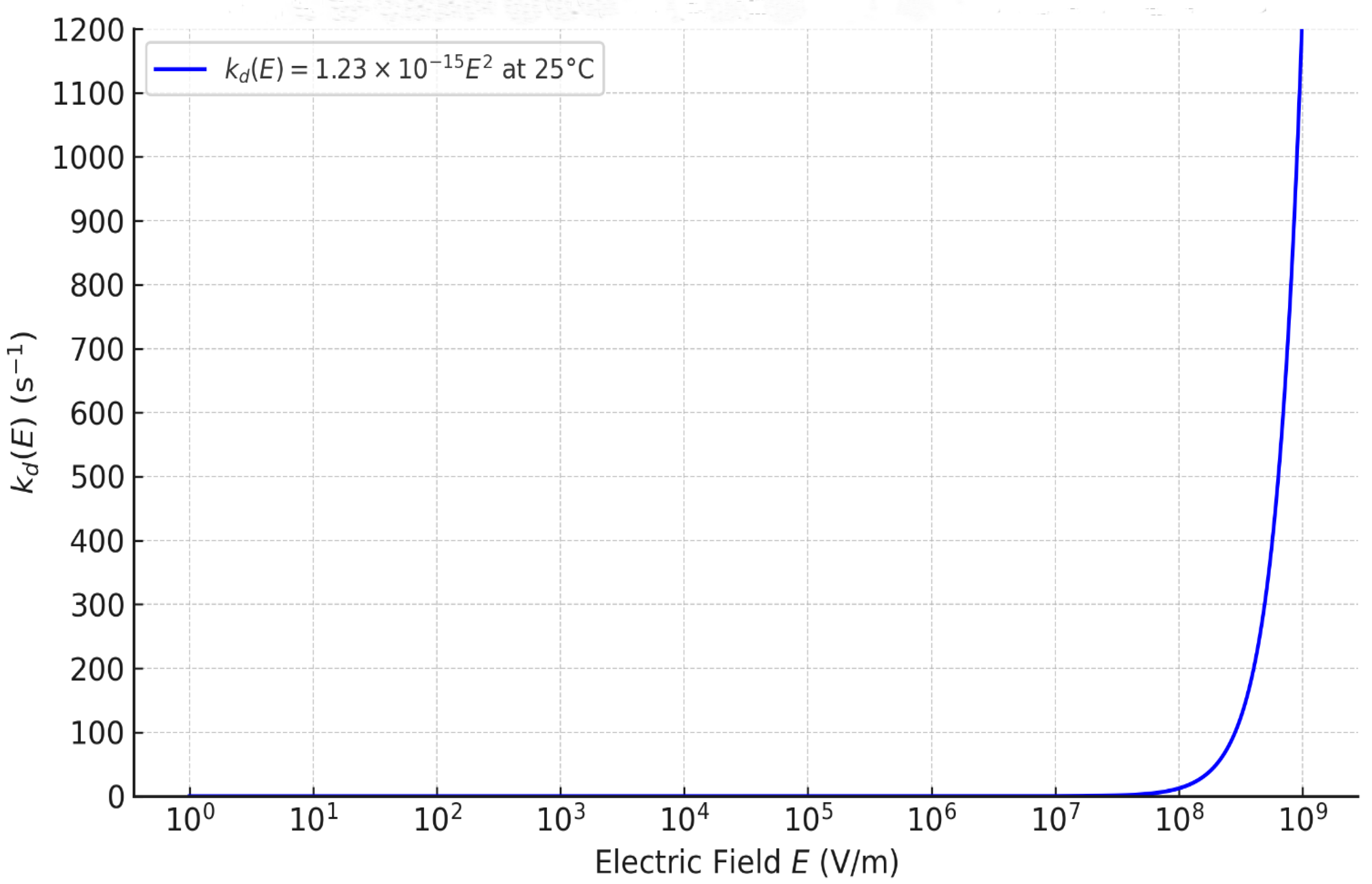
Figure 2.
Theoretical J–Uⱼ curve of a nanometric BPM junction fully hydrated obtained from J = 660 2.
Figure 2.
Theoretical J–Uⱼ curve of a nanometric BPM junction fully hydrated obtained from J = 660 2.
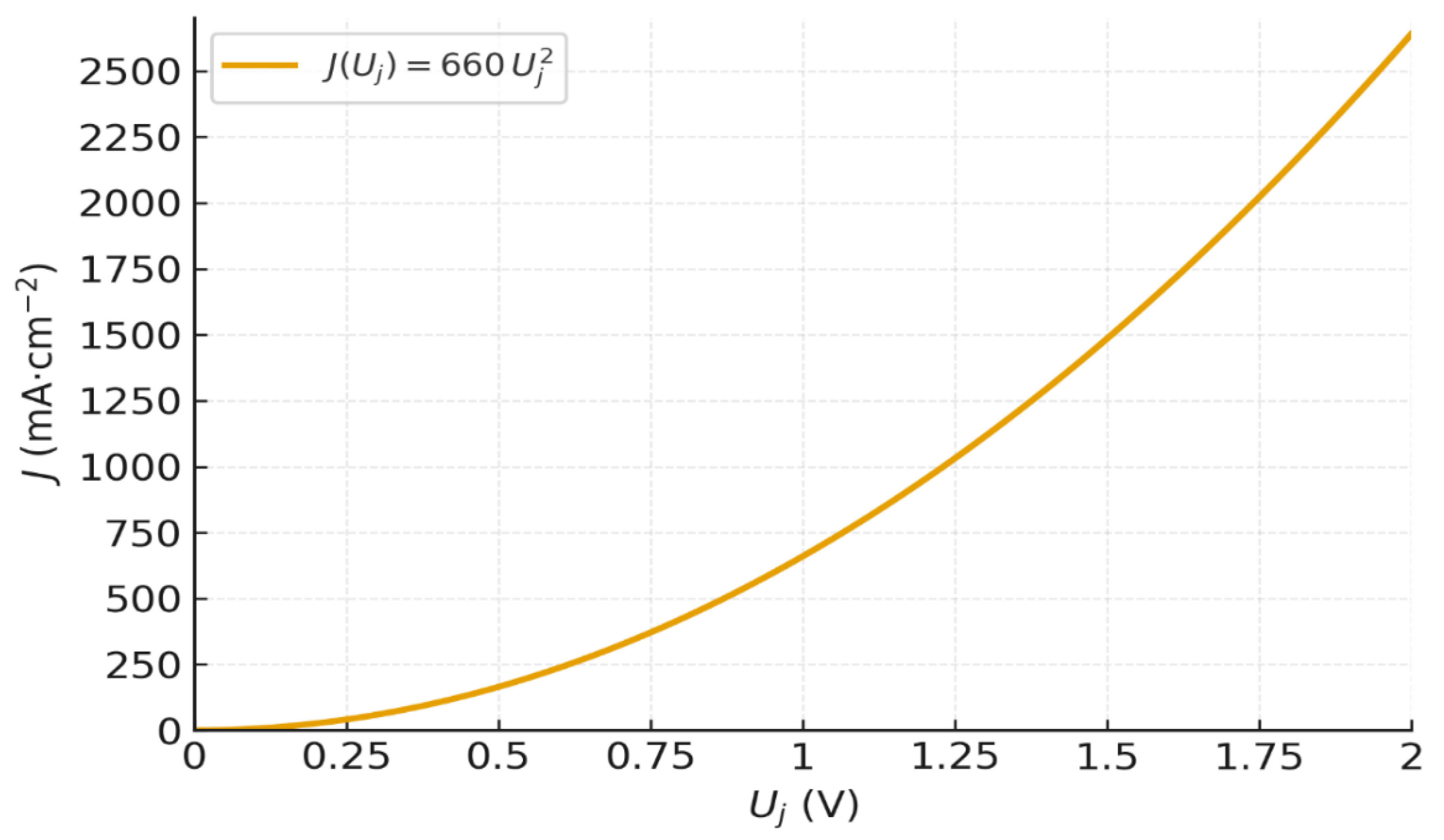
Figure 3.
Raw J vs curve of Fumasep® FBM obtained from LSV measurement.
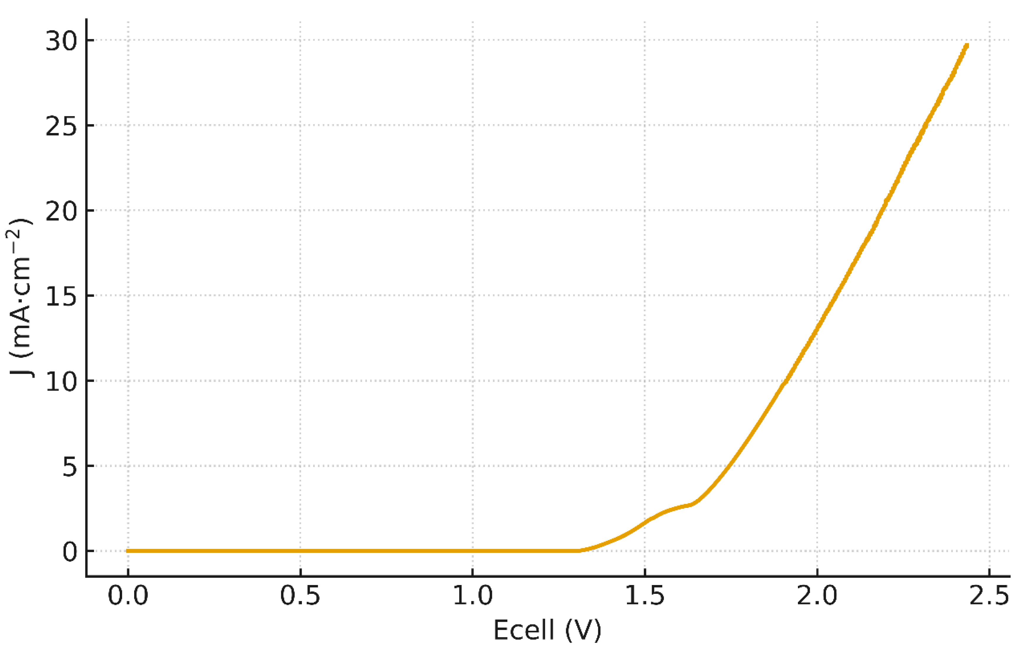
Figure 4.
Fits over 1.36V-1.54V of J vs Ecell : a) Linear fit ; b) Quadratic fit.
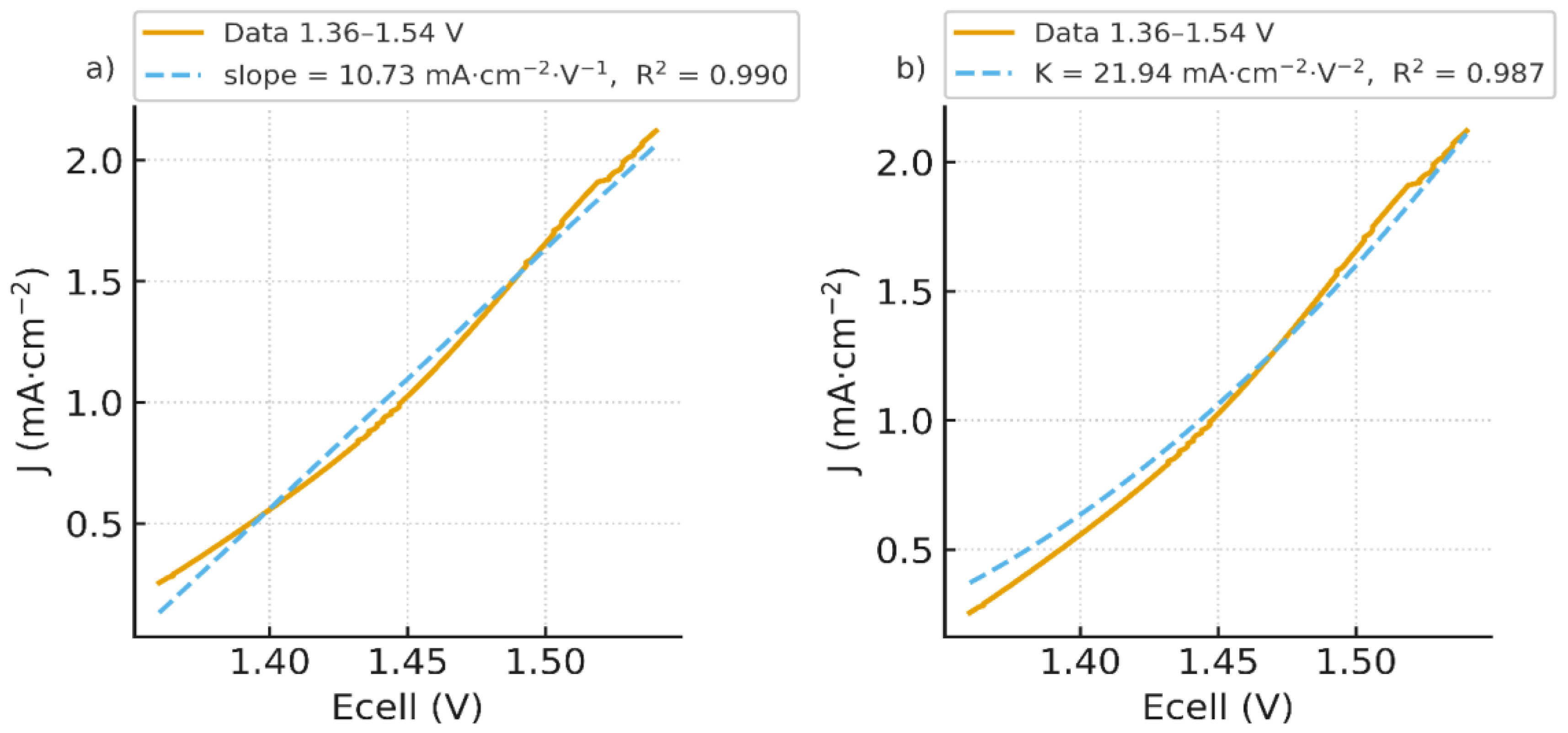
Figure 5.
Variation of the current density J vs , quadratic fit J vs and limiting-current density J = 2.19 mA·cm⁻².
Figure 5.
Variation of the current density J vs , quadratic fit J vs and limiting-current density J = 2.19 mA·cm⁻².
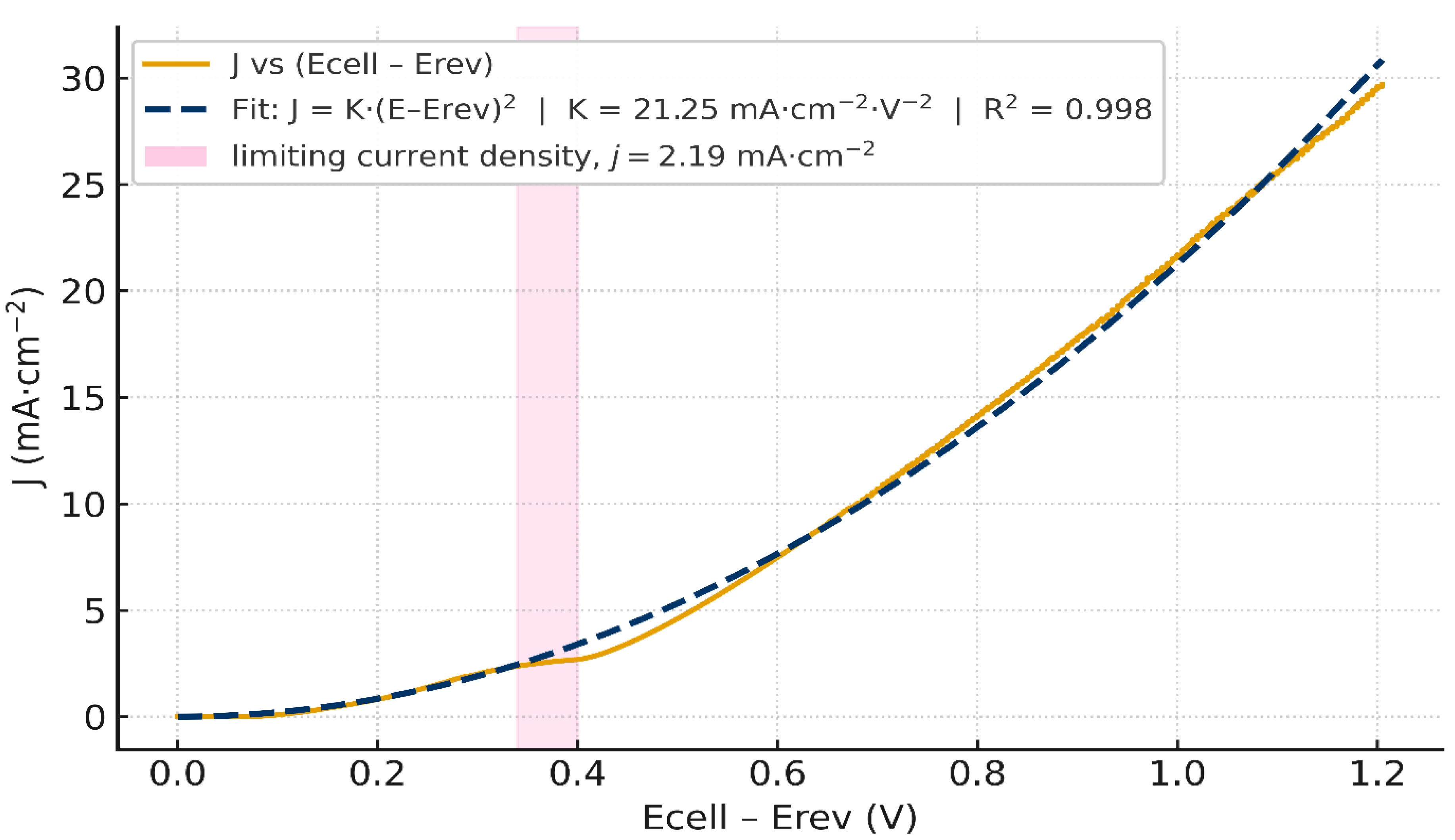
Figure 6.
a) Nyquist plot from (EIS) of the FBM H-cell (VersaSTAT 4A) with Zoom on HF-intercept = 20.19 Ω·cm² ; b) Raw J vs Ecell curves (LSV) for the FBM H-cell together with iRs-corrected by the cell-level = 20.19 Ω·cm².
Figure 6.
a) Nyquist plot from (EIS) of the FBM H-cell (VersaSTAT 4A) with Zoom on HF-intercept = 20.19 Ω·cm² ; b) Raw J vs Ecell curves (LSV) for the FBM H-cell together with iRs-corrected by the cell-level = 20.19 Ω·cm².
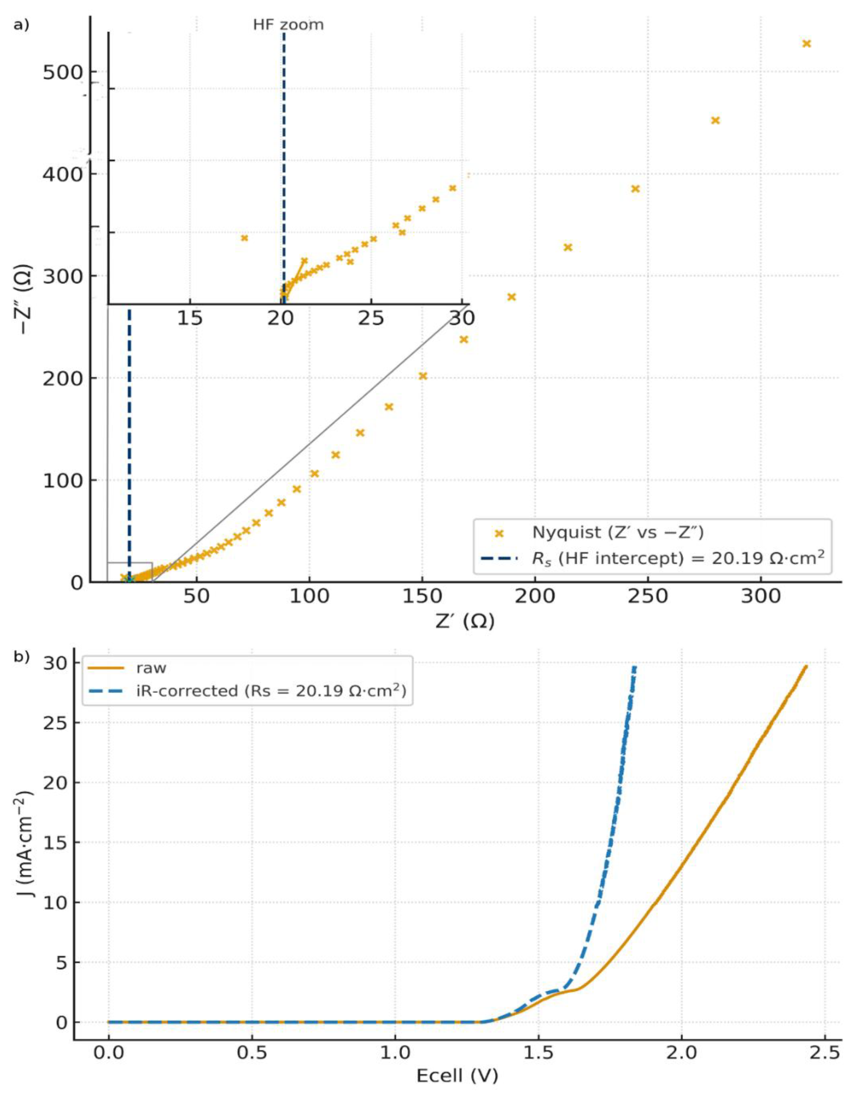
Figure 7.
a) HER polarization curves (raw and iR-corrected) : Pt in 0.5 M H₂SO₄ vs Hg/HgSO₄ (reported vs RHE); b) OER polarization curves (raw and iR-corrected) : Ni-foam in 1.0 M NaOH vs Hg/HgO (vs RHE); c) HER Tafel plot = -29.66 mV·dec⁻¹; = 9.20×10⁻⁴ A·cm⁻² ; d) OER Tafel plot = 41.92 mV·dec⁻¹; = 6.11×10⁻¹⁰ A·cm⁻².
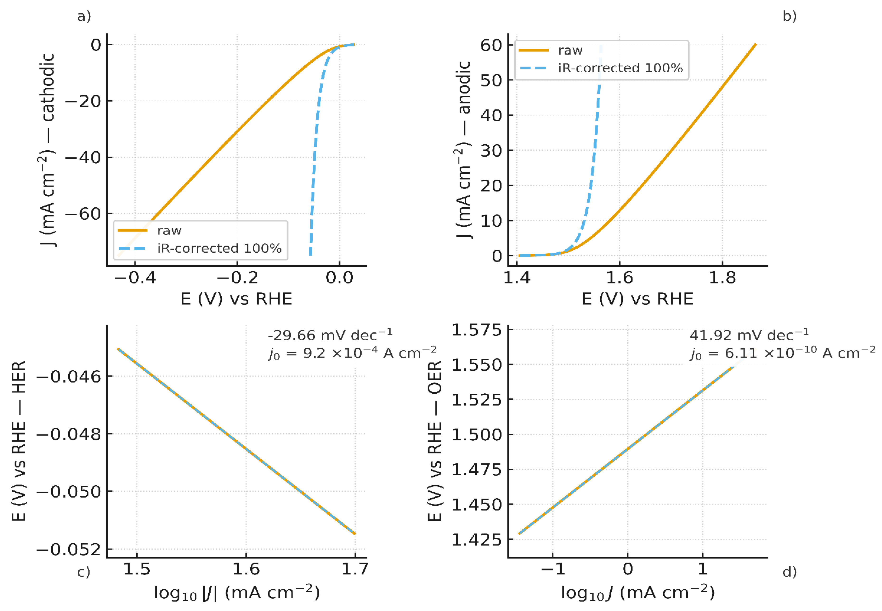
Figure 8.
Quadratic fit of J vs Uj curve obtained from Eq.(33) : ≃
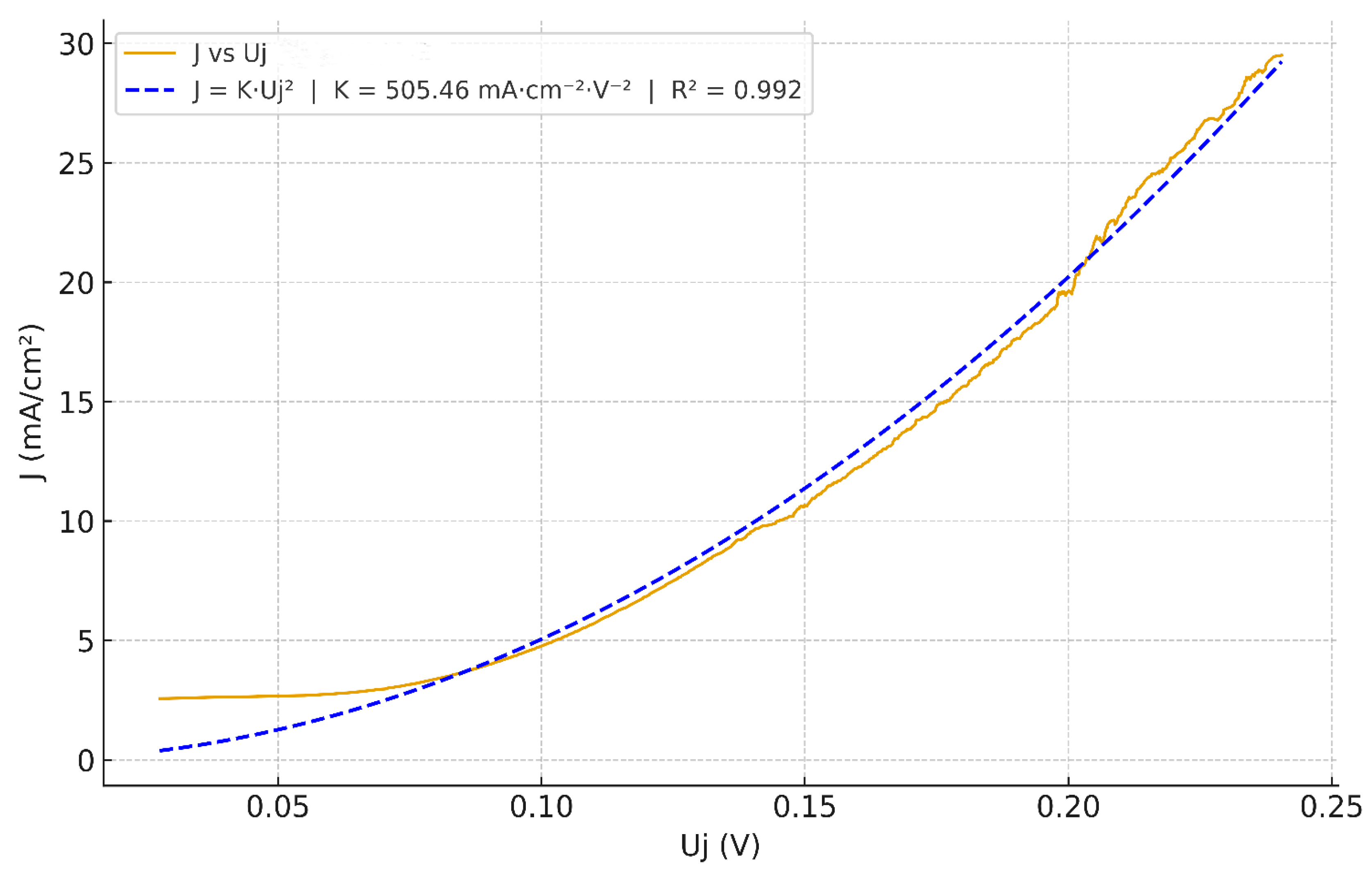

Table 1.
Values of kd as a function of E, according to equation (31) of our model.
| Electric Field, E (V·m⁻¹) | WD rate, (E) (s-1) | Ratio increase, / |
| 1 × 10⁸ | 12.3 | 4.92 × 10⁵ |
| 5 × 10⁸ | 307 | 1.23 × 10⁷ |
| 8 × 10⁸ | 787 | 3.15 × 10⁷ |
| 1 × 10⁹ | 1230 | 4.92 × 10⁷ |
| 2 × 10⁹ | 4920 | 1.97 × 10⁸ |
Table 2.
Comparison of values obtained with our model and SWE model.
| Model |
for E = 10⁸ V·m⁻¹ |
for E = 2×10⁹ V·m⁻¹ |
Commentary |
|---|---|---|---|
| =78) | 3.67 | 4.07×10⁴ | Too slow |
| variable) | 3.67 | 8.05×10¹¹ | Improved but unstable |
| =10) | 3.07×10² | 3,43×10¹⁵ | Divergence |
| =5) | 8.61×10³ | 6.18× | Extreme divergence |
| Our quadratic model | 4.92×10⁵ | 1.97×10⁸ | Gradual, realistic increase |
Disclaimer/Publisher’s Note: The statements, opinions and data contained in all publications are solely those of the individual author(s) and contributor(s) and not of MDPI and/or the editor(s). MDPI and/or the editor(s) disclaim responsibility for any injury to people or property resulting from any ideas, methods, instructions or products referred to in the content. |
© 2025 by the authors. Licensee MDPI, Basel, Switzerland. This article is an open access article distributed under the terms and conditions of the Creative Commons Attribution (CC BY) license (http://creativecommons.org/licenses/by/4.0/).
Copyright: This open access article is published under a Creative Commons CC BY 4.0 license, which permit the free download, distribution, and reuse, provided that the author and preprint are cited in any reuse.


