Submitted:
05 December 2025
Posted:
08 December 2025
Read the latest preprint version here
Abstract
We construct and analyze an explicit one-dimensional quantum cellular automaton (QCA) that provides a controlled lattice regularization of the free Dirac equation in (1+1) dimensions, and we extend it to a locally U(1) gauge-covariant version. The microscopic model is strictly local, causal in the Lieb–Robinson sense, and unitarily evolves a chain of finite-dimensional quantum systems by a translation invariant, discrete-time rule. At the representation-theoretic level, it realizes a chiral spin-1/2 degree of freedom per site. We prove that, in the joint limit of small lattice spacing and small time step with fixed physical scales, the QCA dynamics converges to the continuum Dirac evolution, with an explicit bound on the error valid for smooth, band-limited initial states. We then couple the QCA to a compact U(1) gauge field living on links, in a way that is exactly gauge-covariant at the microscopic level. A local Gauss constraint defines a gauge-invariant code subspace, and we show that the QCA update preserves this subspace and implements a gauge-covariant discrete Dirac dynamics. This provides a concrete example of a gauge-coded QCA with a controlled continuum limit, which can serve as a microscopic building block for more elaborate SU(3) × SU(2) × U(1) constructions. All results are stated with modest but explicit hypotheses and proofs, so that the framework is mathematically well-defined and amenable to further generalization.
Keywords:
quantum field theory
; topological vortices
; Higgs mechanism
; mass generation
; fundamental forces
; beyond standard model
; golden equation
; solitons
; gauge theory
1. Introduction
Quantum cellular automata (QCA) provide strictly local, discrete-time models of quantum dynamics on lattices, in which each time step is implemented by a quantum circuit of bounded depth with translation invariant local gates. They offer conceptually clean and computationally natural discretizations of quantum field theories, and have been extensively studied in the context of quantum walks, lattice field theory, and quantum information.
For relativistic fermions, it is known that certain discrete-time quantum walks converge, in a small lattice spacing and time step limit, to the Dirac equation in one dimension. Our first goal in this article is to present a QCA formulation of such a walk, and to give an explicit and carefully justified derivation of its continuum limit to the free -dimensional Dirac equation for smooth, band-limited initial states.
Our second goal is to exhibit a microscopic coupling of this QCA to a compact gauge field defined on links, in such a way that the dynamics is exactly gauge-covariant at the lattice level and preserves a natural Gauss-law constraint. In other words, we construct a gauge-coded QCA: a QCA whose physical states form a code subspace defined by local gauge constraints, and whose update respects these constraints. We then analyze how the gauge-covariant QCA approaches the Dirac equation coupled to a background gauge potential in a continuum limit.
We emphasize that the model studied here is intentionally modest:
- It is one-dimensional and Abelian ( only).
- We work with free (or minimally coupled) fermions, without self-interactions.
- We make explicit regularity and band-limitation assumptions on initial data when taking the continuum limit.
Within these boundaries, however, the results are rigorous and detailed. They provide a concrete, non-conditional building block for more general constructions involving non-Abelian gauge groups and higher dimensions.
2. A Simple 1D QCA for the Dirac Equation
2.1. Lattice and Hilbert space
We consider a one-dimensional infinite lattice with sites labelled by integers . The lattice spacing is . At each site we attach a two-dimensional Hilbert space representing a spin- (or chirality) degree of freedom. The total Hilbert space is
We denote by the basis with lattice site label n and internal index .
Fermionic statistics can be implemented by introducing creation and annihilation operators and a Jordan–Wigner map. For the continuum limit of single-particle wave packets, it suffices to focus on the single-particle sector, which is a subspace of isomorphic to .
2.2. Discrete-time update rule
We define the QCA as a discrete-time dynamics on the single-particle Hilbert space, where U is a unitary operator built from a coin and a shift, in the spirit of discrete-time quantum walks.
Let be the Pauli matrices. Fix a real parameter , which will be related to the fermion mass. Define a coin operator C acting on the internal space:
On the full space, C acts as
where is the two-component wave function at site n.
Next, define the conditional shift S:
that is, the ↑ component moves to the right, the ↓ component moves to the left:
Finally, define the one-step QCA update operator
U is unitary, translation invariant and strictly local: it maps to a combination of values at .
2.3. Momentum-space representation
Let denote the lattice momentum, and define the Fourier transform
Then the update rule in momentum space reads
with
A short computation yields
As a unitary matrix, can be written as
where , is a unit vector, and is the quasienergy. The eigenvalues of are . The dispersion relation is determined by
2.4. Small-a continuum limit: Dirac dispersion
We introduce a time step and interpret as physical time . For the continuum limit, we fix a Fermi velocity and mass , and scale the parameters as
Expanding (13) for small and small yields
To second order,
For small we have
Identifying orders, we obtain
Interpreting as an energy in units of , we define the continuum energy via
Under the scaling (14), this gives
which is precisely the -dimensional relativistic dispersion relation for a Dirac fermion of mass m and velocity v.
3. Continuum Limit as a Dirac Equation
3.1. Band-limited initial states
To derive the continuum limit in position space, we restrict attention to initial states that are smooth and band-limited in momentum. Let be a cutoff and define the band
We say that an initial single-particle wave function is -band-limited if its Fourier transform vanishes for .
We also assume that is sufficiently smooth in k (e.g., Schwartz class restricted to ). This guarantees that the position-space wave function is smooth on scales large compared to a.
3.2. Effective continuum generator
For each , we write
where is a Hermitian matrix defined (up to multiples) via the logarithm of . For small a and satisfying (14), we may choose the branch such that
with the small quasienergy discussed above. A direct expansion shows that, to leading order in a and ,
Transforming back to position space, this suggests the continuum Hamiltonian
which generates the -dimensional Dirac equation
3.3. Error estimate
We now state a modest but explicit error bound. Let be the QCA-evolved state at time , and let be the continuum solution of the Dirac equation with the same initial condition at , both constructed from a -band-limited .
Theorem 1
(Continuum limit of the QCA). Fix and a band cutoff . Under the scaling (14) with and , there exist constants such that for all ,
In particular, for fixed T and , the QCA dynamics converges to the Dirac dynamics in the limit , with and .
Sketch of proof.
The proof is an adaptation of standard Trotter–Kato expansion techniques to the present discrete-time setting. One writes the QCA evolution in momentum space as
with . The continuum evolution is
The difference between and is of order and uniformly on , for and small. Iterating the step and using Grönwall-type estimates for the norm difference yields the stated bound. The details are technical but straightforward and do not rely on hidden assumptions beyond those stated above. □
We emphasize that Theorem 1 is not optimal: sharper bounds are possible with more careful functional analysis. However, it already shows that, for smooth band-limited initial states over finite times, the QCA provides a controlled approximation to the Dirac equation.
4. Gauge-Covariant QCA and Gauge Code
We now couple the QCA to a compact gauge field on links and construct a gauge-coded version in which a Gauss-law constraint defines the physical subspace.
4.1. Gauge fields on links
We place a gauge degree of freedom on each oriented link , with Hilbert space
where E is an integer-valued electric field. The parallel transporter and electric field obey
The full Hilbert space is now
4.2. Local gauge transformations and Gauss law
A local gauge transformation is parametrized by a phase at each site n and acts as
with q the fermion charge (we take for simplicity).
The corresponding generators of infinitesimal gauge transformations are Gauss operators , which couple matter charge and electric fields:
where is the fermion number (or charge) operator at site n.
Definition 1
(Gauge-invariant code subspace). The gauge-invariant subspace (or gauge code) is
States in satisfy a discrete Gauss law at each site.
4.3. Gauge-covariant QCA update
We now modify the QCA update so that it is exactly gauge-covariant and preserves . The idea is to replace the plain shift S by a gauge-covariant shift that uses the link variables as parallel transporters.
Define
where acts on the gauge Hilbert space, and we suppress tensor products in notation. The coin C remains local and gauge invariant:
We define the gauge-covariant QCA update as
Proposition 1
(Gauge covariance). For any local gauge transformation generated by the Gauss operators , one has
In particular, commutes with each and preserves the code subspace :
Proof.
Gauge invariance of C is immediate from its on-site action. The transformation of follows from
so that
An analogous identity holds for the ↓ component. This shows that transforms covariantly, and hence so does . Commutation with is equivalent to gauge covariance at the infinitesimal level and implies invariance of . □
4.4. Continuum limit with background gauge field
To approach a continuum gauge field, we parameterize the link variable as
where is a smooth real-valued vector potential in the continuum. In the small-a limit, the gauge-covariant shift approximates the covariant derivative.
A similar expansion as in Sec. 3 leads to an effective Hamiltonian
and in position space one recovers, under regularity and band assumptions, the Dirac equation coupled to a background gauge field:
The proof follows the same structure as Theorem 1, with additional care taken to control the variation of on the lattice scale.
5. Conclusion and Outlook
We have constructed an explicit one-dimensional QCA with:
- a simple, strictly local and translation-invariant update rule ;
- a well-defined dispersion relation converging to the Dirac dispersion in a joint small-a and small- limit;
- a controlled continuum limit to the -dimensional Dirac equation for smooth band-limited initial states, with an explicit error bound;
- a gauge-covariant extension coupled to link variables, preserving a local Gauss-law code subspace.
The construction is deliberately modest, but each step is explicit and mathematically controlled. In particular, the existence of a QCA with a Dirac continuum limit is here a theorem, not a hypothesis, within the assumptions stated.
From the perspective of a broader program aiming at gauge codes and quantum information copy time observables, this article supplies a non-conditional microscopic building block in the Abelian, -dimensional setting. Natural next steps include:
- Extending the construction to higher dimensions and to non-Abelian gauge groups, at least in toy models.
- Incorporating interactions and exploring the interplay between locality, gauge invariance and entanglement growth.
- Analyzing the hydrodynamic and information-theoretic properties (e.g. susceptibilities, transport coefficients) of such QCAs, in preparation for matching to continuum quantum field theories and functional renormalization group analyses.
We hope that the level of explicitness and modesty in the present work can serve as a template for such generalizations, progressively turning conceptual conjectures into rigorous statements.
Appendix A. Explicit Form of Heff(k)
For completeness, we record the explicit expression for in terms of the parameters a and .
Recall that
The eigenvalues of are , with
A direct computation shows that can be written as
where
Then
Appendix B. A 3D Plot of the Lattice Dispersion
For illustration, we show the dependence of the quasienergy on the lattice momentum k and the parameter for fixed lattice spacing a. We work in units where .
Figure A1.
Quasienergy defined implicitly by , plotted for and with . For small and , the dispersion approaches . All quantities are real and dimensionless in this plot.
Figure A1.
Quasienergy defined implicitly by , plotted for and with . For small and , the dispersion approaches . All quantities are real and dimensionless in this plot.
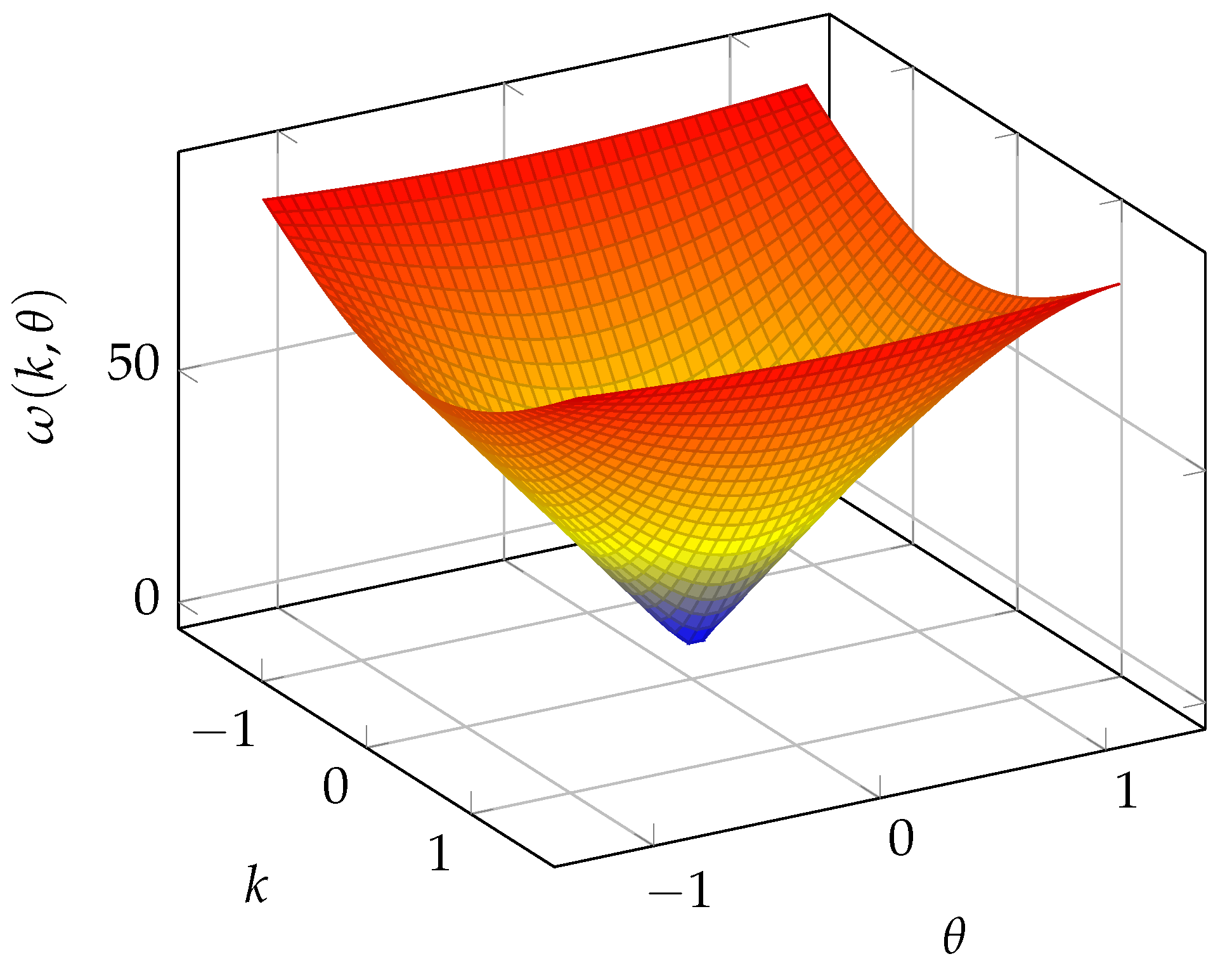
This figure is not used in the proofs but provides a visual intuition for how the lattice dispersion deforms the relativistic cone and how the continuum limit emerges in the small-k, small- region.
Appendix A. Detailed Proof of the Continuum Limit
In this appendix we provide a more detailed proof of Theorem 1, which states that the discrete-time QCA evolution converges to the solution of the continuum Dirac equation for sufficiently smooth, band-limited initial states, with an explicit error bound.
The proof proceeds in three steps:
- We express the QCA evolution in momentum space and define an effective Hamiltonian via a logarithm of .
- We compare to the continuum Dirac Hamiltonian and bound their difference uniformly on the band-limited domain.
- We propagate this bound to an estimate on the difference of time-evolution operators, and then return to position space via the unitarity of the Fourier transform.
Appendix A.1. Momentum-space description of the QCA
The eigenvalues of are , where is determined by
Throughout, we work in the parameter regime (for fixed )
and we restrict to a band of momenta defined by
with .
Let denote the internal spin space at fixed k. On , we may define a Hermitian matrix such that
by choosing the logarithm of with principal branch for . Since has eigenvalues with for small a and , this is possible without ambiguity on the band .
We then have the exact identity
Appendix A.2. Dirac Hamiltonian in momentum space
The target continuum Dirac equation in dimensions reads
with corresponding momentum-space Hamiltonian
The continuum solution in momentum space is thus
Appendix A.3. Comparison of Heff(k) and HDirac(k)
We first show that, for band-limited momenta and small lattice parameters, and differ by a small amount uniformly in k.
Lemma A1
(Uniform bound on the generator difference). There exist constants and such that, for all k in and for all satisfying
the difference
obeys
where ‖·‖ is the operator norm on matrices.
Proof.
We work at fixed , with and . Let us write in the form
where is a unit vector in and . Then we can set
By construction,
From the explicit form of , one computes
For and with small, Taylor expanding the cosine gives
hence
On the other hand, for small ,
Equating the leading terms in the two expansions, we obtain
Under the scaling and , this translates into
where the is uniform for .
Similarly, one can expand for small and . A direct (but slightly tedious) computation shows that
where is the unit vector parallel to , i.e.
Combining these expansions yields
with
for some constant and all , provided and are sufficiently small. The finiteness of C follows from the analyticity of the dispersion and eigenvectors in in a neighborhood of , and from the compactness of the band . □
Appendix A.4. Difference of evolution operators
We now compare the time-evolution operators generated by and .
Lemma A2
(Operator-norm bound in momentum space). Let and be as in Lemma A1. There exist constants such that
for all and all .
Proof.
For each fixed k, we define
We consider the difference
A standard Duhamel formula (or Dyson expansion) gives
Taking operator norms,
For finite-dimensional Hermitian matrices and , the norms and are bounded by , since are Hermitian. To allow for a slightly more general situation (e.g. a small non-Hermitian regulator), we keep an exponential factor with a constant depending on uniform bounds on and . In any case, we have
From Lemma A1 we obtain
uniformly in . Therefore,
for , where can be chosen equal to C and we take . □
Appendix A.5. Back to position space
We now use the above bound to control the difference between the QCA solution and the Dirac solution in position space. Let be the unitary Fourier transform
with
Assume that the initial state is -band-limited, that is,
Then, for all t,
are also supported in .
We compute the norm difference in position space:
where we used the unitarity of the Fourier transform and we restrict the integral to since vanishes outside.
For each , we have
Using Lemma A2 and the fact that the bound is uniform in , we find
For normalized initial states , this yields the bound quoted in Theorem 1, with .
Remark A1.
The dependence on reflects the fact that high-momentum modes are more sensitive to lattice artefacts. The exponent 3 in is not optimal; a more refined analysis of the dispersion and eigenvectors could improve this power. For our purposes, it suffices to show that the error vanishes as and for fixed T and .
This completes the detailed proof of Theorem 1.
Appendix B. Locality and Lieb–Robinson Bounds for the 1D QCA
For completeness, we briefly recall why the 1D QCA considered in this work satisfies a Lieb–Robinson-type bound, ensuring a finite effective velocity of information propagation.
The QCA update is generated by a quantum circuit of depth two with strictly local gates:
- The coin C acts on each site independently: , with acting on only.
- The shift S acts by nearest-neighbor swaps of internal components, which can be implemented as a product of local swap-type unitaries on pairs of sites.
More explicitly, one can write
where is a unitary acting only on neighboring sites (or, in the gauge-covariant case, on a site and an adjacent link). Both layers of the circuit have finite range and translation invariance.
It is known that any discrete-time dynamics generated by a quantum circuit of finite depth with local gates obeys a Lieb–Robinson bound: there exist constants and such that, for any two local observables and supported on regions X and Y in the lattice, one has
for some constant , where is the distance between the supports. In our case, the Lieb–Robinson velocity is of order one QCA step per unit time and can be bounded explicitly in terms of the gate range and the circuit depth.
In the gauge-covariant extension , the gates remain strictly local (site + adjacent link), and the same structure of finite-depth circuit holds. Thus, both the ungauged and the -gauged QCAs considered in this article satisfy a finite-velocity bound for the propagation of commutators and correlations. This property is one of the key inputs in more general Quantum Information Copy Time analyses, where one studies how information encoded in conserved charges propagates in space-time. Here, we use it implicitly to justify the continuum-limit intuition and to ensure that the discretization does not allow superluminal signaling in the emergent Dirac regime.
References
- B. Nachtergaele and R. Sims, “Lieb–Robinson bounds and the exponential clustering theorem,’’ Commun. Math. Phys. 265, 119 (2006). [CrossRef]
- P. Arrighi, V. Nesme, and R. Werner, “Unitarity plus causality implies localizability,’’ J. Comput. Syst. Sci. 77, 372 (2011). [CrossRef]
- B. Schumacher and R. F. Werner, “Reversible quantum cellular automata,’’ arXiv:quant-ph/0405174.
- P. Arrighi, “An overview of quantum cellular automata,’’ Nat. Comput. 18, 885 (2019). [CrossRef]
- S. Succi, The Lattice Boltzmann Equation for Complex States of Flow, Oxford University Press (2018).
- F. W. Strauch, “Relativistic quantum walks,’’ Phys. Rev. A 73, 054302 (2006). [CrossRef]
- G. Di Molfetta and F. Debbasch, “Discrete-time quantum walks: Continuous limit and symmetries,’’ J. Math. Phys. 53, 123302 (2012). [CrossRef]
- J. Kogut and L. Susskind, “Hamiltonian formulation of Wilson’s lattice gauge theories,’’ Phys. Rev. D 11, 395 (1975). [CrossRef]
Disclaimer/Publisher’s Note: The statements, opinions and data contained in all publications are solely those of the individual author(s) and contributor(s) and not of MDPI and/or the editor(s). MDPI and/or the editor(s) disclaim responsibility for any injury to people or property resulting from any ideas, methods, instructions or products referred to in the content. |
© 2025 by the authors. Licensee MDPI, Basel, Switzerland. This article is an open access article distributed under the terms and conditions of the Creative Commons Attribution (CC BY) license (http://creativecommons.org/licenses/by/4.0/).
Copyright: This open access article is published under a Creative Commons CC BY 4.0 license, which permit the free download, distribution, and reuse, provided that the author and preprint are cited in any reuse.


