Electromagnetic Sources Teleparallel Robertson-Walker F(T)-Gravity Solutions

1. Introduction

The teleparallel $F\left(T\right)$ gravity is a frame-based alternative theory to general relativity (GR) defined in terms of a coframe/spin-connection pair (${\mathbf{h}}^a$–${\omega }_{bc}^a$ pair) [1,2,3,4,5,6,7]. The two last quantities define the torsion tensor $T_{bc}^a$ and torsion scalar T. We remind that GR is defined by the metric $g_{\mu \nu }$ and the spacetime curvatures $R_{b\mu \nu }^a$, $R_{\mu \nu }$ and R. We can determine the symmetries for any independent coframe/spin-connection pairs, and then spacetime curvature and torsion are defined as geometric objects [4,5,6,7,8,9]. Any geometry described by a such pair whose curvature and non-metricity are zero ($R_{b\mu \nu }^a=0$ and $Q_{a\mu \nu }=0$ conditions) is a teleparallel gauge-invariant geometry (for any gauge metric $g_{ab}$). The fundamental pairs must satisfy two Lie derivative-based relations and we use the Cartan–Karlhede algorithm to solve the two fundamental equations for any teleparallel geometry. For a pure teleparallel $F\left(T\right)$ gravity spin-connection solution, we solve the null Riemann curvature condition leading to a Lorentz transformation-based definition of ${\omega }_{b\mu }^a$. There is a direct equivalent to GR in teleparallel gravity: the teleparallel equivalent to GR (TEGR) generalizing to the teleparallel $F\left(T\right)$-type gravity [7,9,10,11,12]. All these considerations are also adapted for the new general relativity (NGR) (refs. [13,14,15] and refs. therein), the symmetric teleparallel $F\left(Q\right)$-type gravity (refs. [16,17,18,19] and refs. therein) and some extended theories like $F(T,Q)$-type, $F(R,Q)$-type, $F(R,T)$-type, and several other ones (refs. [20,21,22,23,24,25,26,27,28,29] and refs. therein). Therefore we will restrict the current study to the teleparallel $F\left(T\right)$ gravity framework.

There are a huge number of research papers on spherically symmetric spacetime solutions in teleparallel $F\left(T\right)$ gravity using a number of approaches, energy-momentum sources and made for various purposes [30,31,32,33,34,35,36,37,38,39,40,41,42,43,44,45,46,47,48,49,50,51,52,53,54,55,56]. There are a special class of teleparallel spacetime which the field equations (FEs) are purely symmetric: the teleparallel Robertson-Walker (TRW) spacetime [55,56,57,58]. The TRW spacetime is defined in terms of the k-parameter where $k=0$ is a flat cosmological spacetime, $k=\pm 1$ are respectively positive and negative space cosmological curvature [59,60,61,62]. A TRW geometry is described by a $G_6$ Lie algebra group, where the 4th to 6th Killing Vectors (KVs) are proper of this spacetime [56,57]. The main consequence of additional KVs is the trivial antisymmetric parts of FEs. The TRW spacetime structure also exists for the teleparallel $F(T,B)$ gravity extension [63,64,65,66,67]. We found teleparallel $F\left(T\right)$ and $F(T,B)$ solutions for perfect fluid (PF) and scalar field (SF) sources. The SF-based teleparallel $F\left(T\right)$ and $F(T,B)$ solutions are scalar potential independent and only SF dependent [55,63]. There are also non-linear fluid teleparallel $F\left(T\right)$ solutions for polytropic and Chaplygin fluids leading to similar results [58]. But there are further possible sources of energy-momentum which might lead to new teleparallel solutions in $F\left(T\right)$-type and some extensions. We can also add recent papers on static radial-dependent, time-dependent and cosmological teleparallel $F\left(T\right)$ and $F(T,B)$ types solutions suitable for universe and astrophysical models [48,49,50,51,52,55,56,63].

Hovever, for electromagnetic teleparallel solutions, there are a limited number of recent contributions. There are some interesting papers on magnetic teleparallel BH solutions, especially from G.G.L.Nashed [68,69,70,71,72,73]. These papers focus essentially on typical BH solutions and usual electromagnetic situations by solving in TEGR and some primarily cases of teleparallel gravity at the astrophysical scale. Therefore, there is no really direct papers using the TRW-based frame approach leading electromagnetic-based cosmological teleparallel solutions using the coframe/spin-connection pair approach. This last missing is the keypoint justifying new development to this way in cosmological teleparallel $F\left(T\right)$-type gravity.

Ultimately we want to study in detail the electromagnetic TRW cosmological solutions with the physical impacts. Therefore we need at the current stage to find the possible electromagnetic source based teleparallel $F\left(T\right)$ gravity solutions in a Robertson-Walker spacetime (TRW). We had found the TRW geometry and solved the TRW FEs and conservation laws (CL) for PF and SF solutions in teleparallel $F\left(T\right)$ and $F(T,B)$ gravities [55,56,57,58,63]. But we can do further and aim to solve for electromagnetic teleparallel $F\left(T\right)$ solutions as the most suitable next step of development. We will use the same TRW geometry and FEs as defined in Section 2.1 and Section 2.2, adapt the CLs for electromagnetic field in Section 2.3, and then find the new teleparallel $F\left(T\right)$ solutions and graphical comparisons in Section 3. We will then discuss on the impacts of new teleparallel solutions in terms of electromagnetic fields in Section 4.1, and then make guidelines for experimental data based comparisons studies in Section 4.2 before concluding in Section 5.

2. Summary of Teleparallel Gravity and Field Equations

2.1. Teleparallel $F\left(T\right)$-Gravity Theory Field Equations and Torsional Quantities

The teleparallel $F\left(T\right)$-type gravity action integral with any gravitational source is [2,3,5,7,47,48,49,50,51,52,55,58,58]:

$$S_{F\left(T\right)}=\int d^{4}x\left[{\displaystyle \frac{h}{2\kappa }}F\left(T\right)+{\mathcal{L}}_{Source}\right],$$

(1)

where h is the coframe determinant, $\kappa$ is the coupling constant and ${\mathcal{L}}_{Source}$ is the gravitational source term. We will apply the least-action principle on the eqn. (1) to find the symmetric and antisymmetric parts of FEs as [47,48,49,50,51,52,55,58]:

$$\begin{array}{ccc}\hfill \kappa {\mathrm{\Theta }}_{\left(ab\right)}& =& F_T\left(T\right){\stackrel{\circ }{G}}_{ab}+F_{TT}\left(T\right)S_{\left(ab\right)}^{\mu }{𝜕}_{\mu }T+{\displaystyle \frac{g_{ab}}{2}}\left[F\left(T\right)-T{F}_T\left(T\right)\right],\hfill \end{array}$$

(2)

$$\begin{array}{ccc}\hfill 0& =& F_{TT}\left(T\right)S_{\left[ab\right]}^{\mu }{𝜕}_{\mu }T,\hfill \end{array}$$

(3)

with ${\stackrel{\circ }{G}}_{ab}$ the Einstein tensor, ${\mathrm{\Theta }}_{\left(ab\right)}$ the energy-momentum, $g_{ab}$ the gauge metric and $\kappa$ the coupling constant. The torsion tensor $T_{\mu \nu }^a$, the torsion scalar T and the super-potential $S_a^{\mu \nu }$ are defined as [5]:

$$\begin{array}{cc}\hfill T_{\mu \nu }^a=& {𝜕}_{\mu }{h}_{\nu }^a-{𝜕}_{\nu }{h}_{\mu }^a+{\omega }_{b\mu }^a{h}_{\nu }^b-{\omega }_{b\nu }^a{h}_{\mu }^b,\hfill \end{array}$$

(4)

$$\begin{array}{cc}\hfill S_a^{\mu \nu }=& {\displaystyle \frac{1}{2}}\left(T_a^{\mu \nu }+T_a^{\nu \mu }-T_a^{\mu \nu }\right)-h_a^{\nu }{T}_{\lambda }^{\lambda \mu }+h_a^{\mu }{T}_{\lambda }^{\lambda \nu },\hfill \end{array}$$

(5)

$$\begin{array}{cc}\hfill T=& {\displaystyle \frac{1}{2}}{T}_{\mu \nu }^a{S}_a^{\mu \nu }.\hfill \end{array}$$

(6)

Eqn. (4) can be expressed in terms of the three irreducible parts of torsion tensor as:

$$\begin{array}{c}\hfill T_{abc}={\displaystyle \frac{2}{3}}\left(t_{abc}-t_{acb}\right)-{\displaystyle \frac{1}{3}}\left(g_{ab}{V}_c-g_{ac}{V}_b\right)+{ϵ}_{abcd}{A}^d\end{array}$$

(7)

where,

$$\begin{array}{cc}\hfill V_a=& T_{ba}^b,A^a={\displaystyle \frac{1}{6}}{ϵ}^{abcd}{T}_{bcd},t_{abc}={\displaystyle \frac{1}{2}}\left(T_{abc}+T_{bac}\right)-{\displaystyle \frac{1}{6}}\left(g_{ca}{V}_b+g_{cb}{V}_a\right)+{\displaystyle \frac{1}{3}}{V}_c.\hfill \end{array}$$

(8)

We usually solve in teleparallel $F\left(T\right)$ gravity the eqns (2)–(3). Therefore in refs. [55,56,57], we showed that eqn (3) is trivially satisfied despite a non-zero spin-connection, because the teleparallel geometry is purely symmetric. Only the eqns (2) is non-trivial and will be explicitly solved in details.

2.2. Teleparallel Robertson-Walker Spacetime Geometry

Any frame-based geometry in teleparallel gravity on a frame bundle is defined by a coframe/spin-connection pair and a field $\mathbf{X}$. The geometry must satisfy the fundamental Lie Derivative-based equations [5,6,55,56,57,58]:

$${\mathcal{L}}_{\mathbf{X}a}={\lambda }_{ab}^b\mathrm{and}{\mathcal{L}}_{\mathbf{X}}{\omega }_{bc}^a=0,$$

(9)

where ${\omega }_{bc}^a$ is the spin-connection in terms of the differential coframe _a and ${\lambda }_a^b$ is the linear isotropy group component. In addition for a pure teleparallel $F\left(T\right)$-type gravity, we must also satisfy the null Riemann curvature condition $R_{abc}^a=0$. For TRW spacetime geometries on an orthonormal frame, the coframe/spin-connection pair $h_{\mu }^a$ and ${\omega }_{abc}$ solutions are [55,56,57,58] :

$$\begin{array}{cc}\hfill h_{\mu }^a=& Diag\left[1,a\left(t\right){\left(1-k{r}^2\right)}^{-1/2},a\left(t\right)r,a\left(t\right)rsin\theta \right],\hfill \\ \hfill {\omega }_{122}=& {\omega }_{133}={\omega }_{144}=W_1\left(t\right),{\omega }_{234}=-{\omega }_{243}={\omega }_{342}=W_2\left(t\right),\hfill \end{array}$$

(10)

$$\begin{array}{cc}\hfill {\omega }_{233}=& {\omega }_{244}=-{\displaystyle \frac{\sqrt{1-k{r}^2}}{a\left(t\right)r}},{\omega }_{344}={\displaystyle \frac{cot\left(\theta \right)}{a\left(t\right)r}},\hfill \end{array}$$

(11)

where $W_1$ and $W_2$ are depending on k-parameter and defined by:

1.

$k=0$: $W_1=W_2=0$,

2.

$k=+1$: $W_1=0$ and $W_2\left(t\right)=\pm {\displaystyle \frac{\sqrt{k}}{a\left(t\right)}}$,

3.

$k=-1$: $W_1\left(t\right)=\pm {\displaystyle \frac{\sqrt{-k}}{a\left(t\right)}}$ and $W_2=0$.

For any $W_1$ and $W_2$, we will obtain the same symmetric FEs set to solve for each subcases depending on k-parameter. The eqns (10)–(11) were found by solving the eqns. (9) and $R_{b\mu \nu }^a=0$ condition as defined in ref. [5]. These solutions were used in several TRW spacetime based works [55,56,57,58,63]. This spacetime structure is still explanable by a $G_6$ Lie algebra group. The TRW FEs are defined for each k-parameter cases and will lead to additional new teleparallel $F\left(T\right)$ solutions. The FEs defined by eqns. (2)–(3) are still purely symmetric and valid on proper frames as showed in refs. [55,56,57,58]. The eqns. (3) are trivially satisfied and we will solve the eqns. (2) for each k-parameter case.

2.3. Einstein-Maxwell Conservation Law Solutions and Energy Conditions

The canonical energy-momentum and its GR CLs are obtained from ${\mathcal{L}}_{Source}$ term of eqn. (1) as [3,7]:

$$\begin{array}{cc}\hfill {\mathrm{\Theta }}_a^{\mu }=& {\displaystyle \frac{1}{h}}{\displaystyle \frac{\delta {\mathcal{L}}_{Source}}{\delta h_{\mu }^a}},\Rightarrow {\stackrel{\circ }{\nabla }}_{\nu }\left({\mathrm{\Theta }}^{\mu \nu }\right)=0,\hfill \end{array}$$

(12)

where ${\stackrel{\circ }{\nabla }}_{\nu }$ the covariant derivative and ${\mathrm{\Theta }}^{\mu \nu }$ the conserved energy-momentum tensor. The antisymmetric and symmetric parts of ${\mathrm{\Theta }}_{ab}$ are [47,48,49,50,51,52,55]:

$${\mathrm{\Theta }}_{\left[ab\right]}=0,{\mathrm{\Theta }}_{\left(ab\right)}=T_{ab},$$

(13)

where $T_{ab}$ is the symmetric part of ${\mathrm{\Theta }}^{\mu \nu }$. The eqn. (12) also imposes the symmetry of ${\mathrm{\Theta }}^{\mu \nu }$ and then eqns. (13) condition. Eqn. (13) is valid only when the matter field interacts with the metric $g_{\mu \nu }$ defined from the coframe $h_{\mu }^a$ and the gauge $g_{ab}$, and is not directly coupled to the $F\left(T\right)$ gravity. This consideration is only valid for the null hypermomentum case (i.e. ${\mathfrak{T}}^{\mu \nu }=0$) as discussed in refs. [48,49,50,51,52,54,55]. This last condition on hypermomentum is defined from eqns. (2)–(3) as [54]:

$$\begin{array}{c}\hfill {\mathfrak{T}}_{ab}=\kappa {\mathrm{\Theta }}_{ab}-F_T\left(T\right){\stackrel{\circ }{G}}_{ab}-F_{TT}\left(T\right)S_{ab}^{\mu }{𝜕}_{\mu }T-{\displaystyle \frac{g_{ab}}{2}}\left[F\left(T\right)-T{F}_T\left(T\right)\right]=0.\end{array}$$

(14)

There are more general teleparallel ${\mathfrak{T}}^{\mu \nu }$ definitions and ${\mathfrak{T}}^{\mu \nu }\ne 0$ CLs, but this does not really concern the teleparallel $F\left(T\right)$-gravity situation [54,76,77,78].

For a TRW spacetime geometry defined by eqns (10)–(11), the eqn (12) for $\rho ={\rho }_{em}$, $P_r=P_{emr}$ and $P_t=P_{emt}$ fluid equivalent for electromagnetic source is [50,55,56,57]:

$$\begin{array}{c}\hfill {\dot{\rho }}_{em}+H\left(3{\rho }_{em}+P_{emr}+2P_{emt}\right)=0,\mathrm{and}2\left(P_{emr}-P_{emt}\right)+r{𝜕}_r{P}_{emr}=0,\end{array}$$

(15)

where $H={\displaystyle \frac{\dot{a}}{a}}$ is the Hubble parameter. The Einstein-Maxwell Lagrangian and then the energy-momentum tensor are defined as [79,80,81,82]:

$$\begin{array}{cc}\hfill {\mathcal{L}}_{source}=-{\displaystyle \frac{1}{4}}{F}_{\mu \nu }{F}^{\mu \nu }\Rightarrow {\mathrm{\Theta }}_{\mu \nu }=& F_{\mu \alpha }{F}_{\nu }^{\alpha }-{\displaystyle \frac{1}{4}}{g}_{\mu \nu }{F}^2,\hfill \end{array}$$

(16)

where $F_{\mu \nu }={\nabla }_{\mu }{A}_{\nu }-{\nabla }_{\nu }{A}_{\mu }$ is the electromagnetic tensor defined in terms of quadripotential $A_{\mu }$. In terms of electric $\overrightarrow{E}$ and magnetic $\overrightarrow{B}$ field, eqn (16) is defined as:

$$\begin{array}{cc}\hfill {\mathrm{\Theta }}_{\mu \nu }=& \left[\begin{array}{cc}{\displaystyle \frac{E^2+B^2}{2}}& {\left[\overrightarrow{S}\right]}^T\\ \left[\overrightarrow{S}\right]& -\left[{\sigma }_{ij}\right]\end{array}\right],\hfill \end{array}$$

(17)

where $\overrightarrow{S}=\overrightarrow{E}\times \overrightarrow{B}$ is the Poynting vector and ${\sigma }_{ij}=\left(E_i{E}_j-{\displaystyle \frac{{\delta }_{ij}}{2}}{E}^2\right)+\left(B_i{B}_j-{\displaystyle \frac{{\delta }_{ij}}{2}}{B}^2\right)$. The eqn (17) is diagonalizable and can be expressed in terms of density-pressure equivalent expressions. The diagonal form is:

$$\begin{array}{c}\hfill {\mathrm{\Theta }}_{\mu }^a\equiv Diag\left[{\rho }_{em},P_{emr},P_{emt},P_{emt}\right].\end{array}$$

(18)

For any EoS and/or equivalent relationship, there are energy conditions (ECs) to satisfy for any physical system based on a PF [83]:

• Weak Energy Condition (WEC): $\rho \ge 0$, $P_r+\rho \ge 0$ and $P_t+\rho \ge 0$.
• Strong Energy Condition (SEC): $P_r+2P_t+\rho \ge 0$, $P_r+\rho \ge 0$ and $P_t+\rho \ge 0$.
• Null Energy Condition (NEC): $P_r+\rho \ge 0$ and $P_t+\rho \ge 0$.
• Dominant Energy Condition (DEC): $\rho \ge |P_r|$ and $\rho \ge |P_t|$.

By this way, we will verify the physical consistency of all CL solutions found in the current paper.

There are three main cases:

1.

General electromagnetic universe: For any $\overrightarrow{E}\ne \overrightarrow{0}$ and $\overrightarrow{B}\ne 0$, eqn (17) becomes:

$$\begin{array}{cc}\hfill {\mathrm{\Theta }}_{\mu \nu }=& \left[\begin{array}{cccc}{\displaystyle \frac{E^2+B^2}{2}}& S_1& S_2& S_3\\ S_1& -{\sigma }_{11}& -{\sigma }_{12}& -{\sigma }_{13}\\ S_2& -{\sigma }_{12}& -{\sigma }_{22}& -{\sigma }_{23}\\ S_3& -{\sigma }_{13}& -{\sigma }_{23}& -{\sigma }_{33}\end{array}\right].\hfill \end{array}$$

(19)

By setting $E_2=E_3=E_t$ and $B_2=B_3=B_t$, we find that $S_1=S_r=0$, $S_2=-S_3=S_t=0$ leading to $E_r{B}_t=E_t{B}_r$ for consistency. By using the last constraint and then by diagonalisation, we find that $P_{emt}=-P_{emr}={\rho }_{em}={\displaystyle \frac{E^2}{2}}\left(1+{\displaystyle \frac{B_r^2}{E_r^2}}\right)$ and the WEC, SEC, NEC and DEC are all satisfied by the $E^2\ge 0$, $E_r^2\ge 0$ and $B_r^2\ge 0$ conditions. Then eqn (15) becomes:

$$\begin{array}{c}\hfill {\dot{\rho }}_{em}+4H{\rho }_{em}=0,\mathrm{and}4{\rho }_{em}+r{𝜕}_r{\rho }_{em}=0,\end{array}$$

(20)

From the 2nd CL, we will find that ${\rho }_{em}(t,r)={\displaystyle \frac{{\rho }_{em}(t,0)}{r^4}}$. Then the 1st CL solution in terms of torsion scalar T is exactly:

$$\begin{array}{c}\hfill {\rho }_{em}(t\left(T\right),r\left(T\right))={\rho }_{em}\left(T\right)={\displaystyle \frac{{\rho }_{em}\left(0\right)}{r^4\left(T\right)a^4\left(T\right)}}.\end{array}$$

(21)

2.

Pure electric universe $|\overrightarrow{B}|\ll |\overrightarrow{E}|$ limit: Eqn (17) becomes:

$$\begin{array}{cc}\hfill {\mathrm{\Theta }}_{\mu \nu }=& \left[\begin{array}{cc}{\displaystyle \frac{E^2}{2}}& 0\\ 0& \left[{\displaystyle \frac{{\delta }_{ij}}{2}}{E}^2-E_i{E}_j\right]\end{array}\right].\hfill \end{array}$$

(22)

By diagonalization techniques applied on eqn (22) and setting $E_2=E_3=E_t$, we find that $P_{emt}=-P_{emr}={\rho }_{em}={\displaystyle \frac{E^2}{2}}$, and then the ECs are trivially satisfied by the $E^2\ge 0$ condition. The eqns (20)–(21) will still be applicable for a pure electric universe.

3.

Pure magnetic universe $|\overrightarrow{B}|\gg |\overrightarrow{E}|$ limit: Eqn (17) becomes:

$$\begin{array}{cc}\hfill {\mathrm{\Theta }}_{\mu \nu }=& \left[\begin{array}{cc}{\displaystyle \frac{B^2}{2}}& 0\\ 0& \left[{\displaystyle \frac{{\delta }_{ij}}{2}}{B}^2-B_i{B}_j\right]\end{array}\right].\hfill \end{array}$$

(23)

Still by using diagonalization techniques on eqn (23) and setting $B_2=B_3$, we find that $P_{emt}=-P_{emr}={\rho }_{em}={\displaystyle \frac{B^2}{2}}$, and then the ECs are trivially satisfied by the $B^2\ge 0$ condition. The eqns (20)–(21) will still be applicable for a pure magnetic universe.

3. Electromagnetic Teleparallel Field Equations Solutions

The general FEs system for TRW cosmological spacetimes are [55,56,57,58]:

1.

$\mathbf{k}=\mathbf{0}$ flat or non-curved:

$$\begin{array}{cc}\hfill \kappa {\rho }_{em}=& -{\displaystyle \frac{F}{2}}+6H^2{F}_T,\hfill \end{array}$$

(24)

$$\begin{array}{cc}\hfill \kappa ({\rho }_{em}+P_{em,r}+2P_{em,t})=& F-6\left(\dot{H}+2H^2\right)F_T-6H{F}_{TT}\dot{T},\hfill \end{array}$$

(25)

$$\begin{array}{cc}\hfill T=& 6H^2.\hfill \end{array}$$

(26)

The eqn (26) yields to $H=\sqrt{{\displaystyle \frac{T}{6}}}$ and from Section 2.3 results, we will find that $\kappa ({\rho }_{em}+P_{em,r}+2P_{em,t})=2\kappa {\rho }_{em}$. In this case, eqns (24)–(25) become

$$\begin{array}{cc}\hfill 2\kappa {\rho }_{em}=& -F+2T{F}_T,\hfill \end{array}$$

(27)

$$\begin{array}{cc}\hfill 2\kappa {\rho }_{em}=& F-\left(6\dot{H}+2T\right)F_T-\sqrt{6T}{F}_{TT}\dot{T}.\hfill \end{array}$$

(28)

By merging eqns (27)–(28), we find the unified FE:

$$\begin{array}{c}\hfill 0=F-\left(3\dot{H}+2T\right)F_T-\sqrt{{\displaystyle \frac{3}{2}}T}{F}_{TT}\dot{T}.\end{array}$$

(29)

The pure vacuum solution (${\rho }_{em}=0$) to eqn (27) is $F\left(T\right)=F_0\sqrt{T}$. However, for ${\rho }_{em}\ne 0$, we can set $a\left(t\right)=a_0{t}^n$ as cosmological scale and consider the radial coordinate $r=r\left(T\right)$ as a complementary function allowing $P_{em,r}\ne P_{em,t}$ situations. Eqn (29) and solutions are:

$$\begin{array}{ccc}\hfill & 0=nF+\left({\displaystyle \frac{1-4n}{2}}\right)T{F}_T+T^2{F}_{TT},\hfill & \hfill \end{array}$$

(30)

$$\begin{array}{ccc}\hfill \Rightarrow F\left(T\right)=& F_0\sqrt{T}+F_1{T}^{2n},\hfill & \hfill n\ne {\displaystyle \frac{1}{4}},\end{array}$$

(31)

$$\begin{array}{ccc}\hfill =& F_0\sqrt{T}+F_1\sqrt{T}ln\left(T\right),\hfill & \hfill n={\displaystyle \frac{1}{4}}.\end{array}$$

(32)

Eqns (31)–(32) are double power-law teleparallel solution very similar to those found in some recent Teleparallel Robertson-Walker based papers [55,56,58,63].

2.

$\mathbf{k}=-\mathbf{1}$ negative curved:

$$\begin{array}{cc}\hfill \kappa {\rho }_{em}\left(T\right)=& -{\displaystyle \frac{F}{2}}+6H\left(H+{\displaystyle \frac{\delta \sqrt{-k}}{a}}\right)F_T,\hfill \end{array}$$

(33)

$$\begin{array}{cc}\hfill \kappa ({\rho }_{em}+P_{em,r}+2P_{em,t})=& F-6\left(\dot{H}+H^2+{\left(H+{\displaystyle \frac{\delta \sqrt{-k}}{a}}\right)}^2\right)F_T-6\left(H+{\displaystyle \frac{\delta \sqrt{-k}}{a}}\right)F_{TT}\dot{T},\hfill \end{array}$$

(34)

$$\begin{array}{cc}\hfill T=& 6{\left(H+{\displaystyle \frac{\delta \sqrt{-k}}{a}}\right)}^2.\hfill \end{array}$$

(35)

From eqn (35) and using $a\left(t\right)=a_0{t}^n$ ansatz, we find a characteristic equation yielding to $t\left(T\right)$ solutions:

$$\begin{array}{cc}\hfill & 0={\displaystyle \frac{\delta \sqrt{-k}}{a_0}}{t}^{-n}+n{t}^{-1}-{\delta }_1\sqrt{{\displaystyle \frac{T}{6}}}.\hfill \end{array}$$

(36)

By substitution of $\kappa ({\rho }_{em}+P_{em,r}+2P_{em,t})=2\kappa {\rho }_{em}$ relation and merging eqns (33)–(34), we find the unified FE:

$$\begin{array}{cc}\hfill 0=& F-3\left({\displaystyle \frac{n(n-1)}{t^2\left(T\right)}}+{\displaystyle \frac{2n{\delta }_1}{t\left(T\right)}}\sqrt{{\displaystyle \frac{T}{6}}}+{\displaystyle \frac{T}{6}}\right)F_T+T\left({\displaystyle \frac{n}{t^2\left(T\right)}}+{\displaystyle \frac{n\delta \sqrt{-k}}{a_0}}{t}^{-n-1}\left(T\right)\right)F_{TT}.\hfill \end{array}$$

(37)

The possible solutions of eqn (36) are by using the far future approximation ($t\left(T\right)\gg 1$ as in ref [58], except for $n=1$ subcase):

(a)

$\mathbf{n}={\displaystyle \frac{\mathbf{1}}{\mathbf{2}}}$ (slow expansion and + solution):

$$\begin{array}{cc}\hfill & t^{-1}\left(T\right)={\left[-{\displaystyle \frac{\delta \sqrt{-k}}{a_0}}\pm \sqrt{-{\displaystyle \frac{k}{a_0^2}}+{\delta }_1\sqrt{{\displaystyle \frac{2T}{3}}}}\right]}^2\approx {\displaystyle \frac{a_0^2}{6(-k)}}T.\hfill \end{array}$$

(38)

By substitution, eqn (37) becomes by neglecting ${\displaystyle \frac{a_0^4}{24{(-k)}^2}}T$ terms:

$$\begin{array}{cc}\hfill 0\approx & F+{\displaystyle \frac{1}{2}}\left({\displaystyle \frac{A^4}{4}}T-A{T}^{1/2}-1\right)T{F}_T+{\displaystyle \frac{A}{12}}\left(A{T}^{1/2}+1\right)T^{5/2}{F}_{TT},\hfill \\ \hfill \Rightarrow F\left(T\right)=& {\displaystyle \frac{1}{\sqrt{T}{\left(1+A\sqrt{T}\right)}^2}}[F_1\left(3A^3{T}^{{\displaystyle \frac{3}{2}}}+10A^{2}T+11A\sqrt{T}+4\right)exp\left(-{\displaystyle \frac{12}{A\sqrt{T}}}\right)\hfill \\ \hfill & +F_2(exp\left(-{\displaystyle \frac{12\left(1+A\sqrt{T}\right)}{A\sqrt{T}}}\right)\left(A^3{T}^{{\displaystyle \frac{3}{2}}}+{\displaystyle \frac{10A^{2}T}{3}}+{\displaystyle \frac{11A\sqrt{T}}{3}}+{\displaystyle \frac{4}{3}}\right)\hfill \\ \hfill & \times {\mathrm{Ei}}_1\left(-{\displaystyle \frac{12\left(1+A\sqrt{T}\right)}{A\sqrt{T}}}\right)+{\displaystyle \frac{119A^3{T}^{\frac{3}{2}}}{1296}}+{\displaystyle \frac{11A^{2}T}{54}}+{\displaystyle \frac{A\sqrt{T}}{9}}\left)\right],\hfill \end{array}$$

(39)

where $A={\displaystyle \frac{{\delta }_1{a}_0^2}{\sqrt{6}(-k)}}$. For the very far future approximation: Eqn (39) becomes $0\approx F-{\displaystyle \frac{T}{2}}{F}_T$ and the solution is $F\left(T\right)\to F_1{T}^2$.

(b)

$\mathbf{n}=\mathbf{1}$ (linear expansion):

$$\begin{array}{cc}\hfill & t^{-1}\left(T\right)={\displaystyle \frac{{\delta }_1}{\left(\frac{\delta \sqrt{-k}}{a_0}+1\right)}}\sqrt{{\displaystyle \frac{T}{6}}}.\hfill \end{array}$$

(40)

By substitution, eqn (37) becomes:

$$\begin{array}{cc}\hfill 0=& F-\left({\displaystyle \frac{1}{\left(\frac{\delta \sqrt{-k}}{a_0}+1\right)}}+{\displaystyle \frac{1}{2}}\right)T{F}_T+{\displaystyle \frac{1}{6\left(\frac{\delta \sqrt{-k}}{a_0}+1\right)}}{T}^2{F}_{TT},\hfill \\ \hfill & \Rightarrow F\left(T\right)=F_1{T}^{r_{+}}+F_2{T}^{r_{-}},\hfill \end{array}$$

(41)

where $r_{\pm }=5+{\displaystyle \frac{3\delta \sqrt{-k}}{2a_0}}\pm \sqrt{19+{\displaystyle \frac{9\delta \sqrt{-k}}{a_0}}-{\displaystyle \frac{9k}{4a_0^2}}}$.

(c)

$\mathbf{n}=\mathbf{2}$ (fast expansion and + solution):

$$\begin{array}{cc}\hfill & t^{-1}\left(T\right)=-{\displaystyle \frac{\delta a_0}{\sqrt{-k}}}\pm \sqrt{-{\displaystyle \frac{a_0^2}{k}}+{\delta }_1\delta a_0\sqrt{-{\displaystyle \frac{T}{6k}}}}\approx {\delta }_1\sqrt{{\displaystyle \frac{T}{24}}}.\hfill \end{array}$$

(42)

By substitution, eqn (37) becomes:

$$\begin{array}{cc}\hfill 0\approx & F-{\displaystyle \frac{7}{4}}T{F}_T+{\displaystyle \frac{1}{12}}{T}^2{F}_{TT},\Rightarrow F\left(T\right)=F_1{T}^{11+\sqrt{109}}+F_2{T}^{11-\sqrt{109}}.\hfill \end{array}$$

(43)

(d)

$\mathbf{n}\to \infty$ (very fast expansion limit):

$$\begin{array}{cc}\hfill & t^{-1}\left(T\right)\approx {\displaystyle \frac{{\delta }_1}{n}}\sqrt{{\displaystyle \frac{T}{6}}}\to 0.\hfill \end{array}$$

(44)

By substitution, eqn (37) becomes $F=2T{F}_T$ and then $F\left(T\right)=F_0\sqrt{T}$. The eqn (33) leads to ${\rho }_{em}\left(T\right)\approx {\displaystyle \frac{F_0\left({\delta }_1-1\right)}{2}}\sqrt{T}=0$ for a positive eqn (44) (i.e. ${\delta }_1=1$), the cosmological vacuum solution, where no electromagnetic field subsists.

3.

$\mathbf{k}=+\mathbf{1}$ positive curved:

$$\begin{array}{cc}\hfill \kappa {\rho }_{em}\left(T\right)=& -{\displaystyle \frac{F}{2}}+6H^2{F}_T,\hfill \end{array}$$

(45)

$$\begin{array}{cc}\hfill \kappa ({\rho }_{em}+P_{em,r}+2P_{em,t})=& F-6\left(\dot{H}+2H^2-{\displaystyle \frac{k}{a^2}}\right)F_T-6H{F}_{TT}\dot{T},\hfill \end{array}$$

(46)

$$\begin{array}{cc}\hfill T=& 6\left[H^2-{\displaystyle \frac{k}{a^2}}\right].\hfill \end{array}$$

(47)

From eqn (47) and using $a\left(t\right)=a_0{t}^n$ ansatz, we find the characteristic equation for $t^{-1}\left(T\right)$:

$$\begin{array}{cc}\hfill & {\displaystyle \frac{k}{a_0^2}}{t}^{-2n}-n^2{t}^{-2}+{\displaystyle \frac{T}{6}}=0.\hfill \end{array}$$

(48)

We simplify and unify by substitution of $\kappa ({\rho }_{em}+P_{em,r}+2P_{em,t})=2\kappa {\rho }_{em}$ the eqns (45)–(46):

$$\begin{array}{cc}\hfill 0=& 2F-\left(6n(3n-1)t^{-2}\left(T\right)+T\right)F_T+12n^2{t}^{-2}\left(T\right)\left(T-6n(n-1)t^{-2}\left(T\right)\right)F_{TT}.\hfill \end{array}$$

(49)

The possible solutions of eqn (48) are with the far future approximation ($t\left(T\right)\gg 1$ as in ref [58], except for $n=1$ subcase):

(a)

$\mathbf{n}={\displaystyle \frac{\mathbf{1}}{\mathbf{2}}}$ (slow expansion and − solution):

$$\begin{array}{cc}\hfill & t^{-1}\left(T\right)={\displaystyle \frac{2k}{a_0^2}}\pm \sqrt{{\displaystyle \frac{4k^2}{a_0^4}}+{\displaystyle \frac{2T}{3}}}\approx -{\displaystyle \frac{a_0^2}{6k}}T.\hfill \end{array}$$

(50)

By substitution, eqn (49) becomes:

$$\begin{array}{cc}\hfill 0\approx & 2F-\left(1+{\displaystyle \frac{a_0^4}{24k^2}}T\right)T{F}_T+{\displaystyle \frac{a_0^4}{12k^2}}\left(1+{\displaystyle \frac{a_0^4}{24k^2}}T\right)T^3{F}_{TT},\hfill \\ \hfill \Rightarrow F\left(T\right)=& exp\left(-{\displaystyle \frac{12k^2}{a_0^{4}T}}\right)\mathrm{HeunC}\left({\displaystyle \frac{1}{2}},1,-1,-{\displaystyle \frac{1}{2}},0,-{\displaystyle \frac{24k^2}{a_0^{4}T}}\right)\hfill \\ \hfill & \times \left[F_1+F_2\int {\displaystyle \frac{exp\left(\frac{12k^2}{a_0^{4}T}\right)dT}{\mathrm{HeunC}{\left(\frac{1}{2},1,-1,-\frac{1}{2},0,-\frac{24k^2}{a_0^{4}T}\right)}^2}}\right].\hfill \end{array}$$

(51)

For the very far future approximation: Eqn (51) becomes $0\approx F-{\displaystyle \frac{T}{2}}{F}_T$ leading to $F\left(T\right)\to F_1{T}^2$ as for the $k=-1$ case.

(b)

$\mathbf{n}=\mathbf{1}$ (linear expansion):

$$\begin{array}{c}\hfill t^{-2}\left(T\right)={\displaystyle \frac{T}{6\left(1-\frac{k}{a_0^2}\right)}}.\end{array}$$

(52)

By substitution, eqn (49) becomes:

$$\begin{array}{cc}\hfill 0=& 2F-\left({\displaystyle \frac{2}{\left(1-\frac{k}{a_0^2}\right)}}+1\right)T{F}_T+{\displaystyle \frac{2}{\left(1-\frac{k}{a_0^2}\right)}}{T}^2{F}_{TT},\hfill \\ \hfill & \Rightarrow F\left(T\right)=F_1{T}^2+F_2{T}^{{\displaystyle \frac{1}{2}}\left(1-{\displaystyle \frac{k}{a_0^2}}\right)}.\hfill \end{array}$$

(53)

(c)

$\mathbf{n}=\mathbf{2}$ (fast expansion and − solution):

$$\begin{array}{cc}\hfill & t^{-2}\left(T\right)={\displaystyle \frac{2a_0^2}{k}}\pm \sqrt{{\displaystyle \frac{4a_0^4}{k^2}}-{\displaystyle \frac{a_0^{2}T}{6k}}}\approx {\displaystyle \frac{T}{24}}.\hfill \end{array}$$

(54)

By substitution, eqn (49) becomes:

$$\begin{array}{cc}\hfill 0\approx & 2F-{\displaystyle \frac{7}{2}}T{F}_T+T^2{F}_{TT},\Rightarrow F\left(T\right)=F_0\sqrt{T}+F_1{T}^4.\hfill \end{array}$$

(55)

(d)

$\mathbf{n}\to \infty$ (very fast expansion limit):

$$\begin{array}{c}\hfill t^{-2}\left(T\right)\approx {\displaystyle \frac{T}{6n^2}}\to 0.\end{array}$$

(56)

By substitution, eqn (49) becomes $F=2T{F}_T$, leading to $F\left(T\right)=F_0\sqrt{T}$ and then eqn (45) becomes $\kappa {\rho }_{em}\left(T\right)=0$ as for the $k=-1$ case, a pure electromagnetic vacuum.

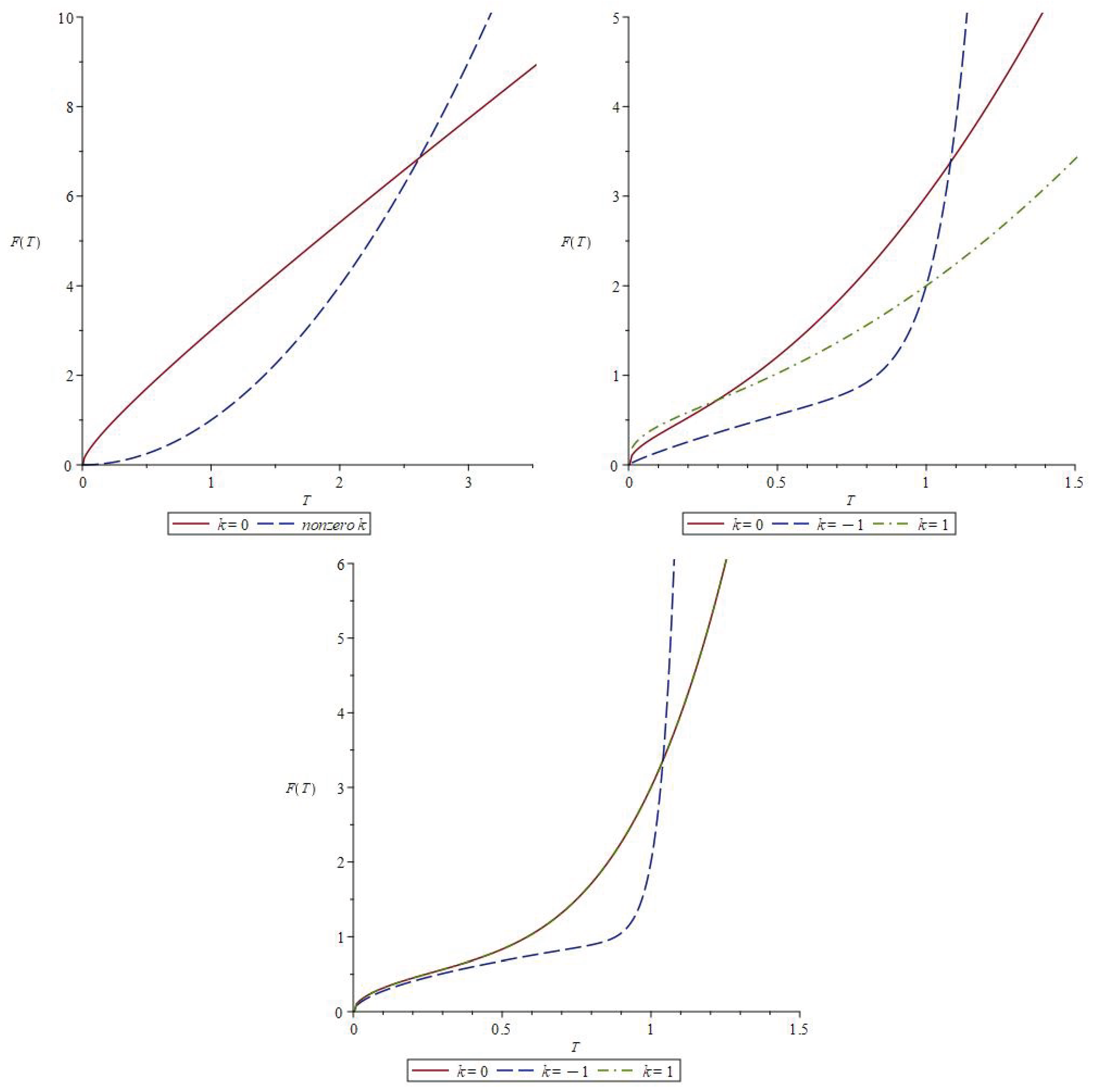
In Figure 1, we compare the new teleparallel $F\left(T\right)$ solutions for highlighting the main common points between solutions. For $n={\displaystyle \frac{1}{2}}$ subcase (slow universe expansion), we find that the $k=\pm 1$ cases lead to the same quadratic $F\left(T\right)$ limit for very far future limit ($t\left(T\right)\gg 1$ approximation), while the $k=0$ case leads to the superposition of TEGR-like term with the large n limit $\sqrt{T}$ term. For the $n=1$ (linear universe expansion) subcase, we find three different curves of teleparallel $F\left(T\right)$ solutions. For $n=2$ subcase (fast universe expansion), we find that $k=0$ and $+1$ cases have the same superposed curves and $k=-1$ is different. However, we have obtained in the current section new simple analytical electromagnetic source-based teleparallel $F\left(T\right)$ solutions suitable for any electromagnetic based universe models.

4. Physical Interpretations and Experimental Data Comparisons

4.1. Electromagnetic Field Interpretations

From the CLs solutions as found in eqn (21), we can find for each new teleparallel $F\left(T\right)$ solution the corresponding electromagnetic field E and/or B. By using the same $a\left(t\right)=a_0{t}^n$ ansatz, the eqn (21) is:

$$\begin{array}{c}\hfill {\rho }_{em}\left(T\right)={\displaystyle \frac{{\tilde{\rho }}_{em}\left(0\right)}{{\left(t^n\left(T\right)r\left(T\right)\right)}^4}},\end{array}$$

(57)

where ${\tilde{\rho }}_{em}\left(0\right)={\displaystyle \frac{{\rho }_{em}\left(0\right)}{a_0^4}}$. We find from eqn (57) that any electromagnetic field will be described by $E\left(T\right)={\displaystyle \frac{E_0}{{\left(a\left(T\right)r\left(T\right)\right)}^2}}$, a Coulombian field, and/or $B\left(T\right)={\displaystyle \frac{B_0}{{\left(a\left(T\right)r\left(T\right)\right)}^2}}$, a magnetic dipole field, with an expanding universe term. In the far future, we find that the electromagnetic fields will be decreasing and then becoming more negligible. But the electromagnetic field as CL solution also needs to satisfy the Maxwell equations as [79,80,81,82]:

$$\begin{array}{cc}\hfill {\nabla }_{\mu }{F}^{\mu \nu }=& J^{\nu },\mathrm{and}{\nabla }_{\kappa }{F}_{\mu \nu }+{\nabla }_{\nu }{F}_{\kappa \mu }+{\nabla }_{\mu }{F}_{\nu \kappa }=0.\hfill \end{array}$$

(58)

We are in principle able to find the four-current $J^{\nu }$ and the four-potential $A^{\nu }$ averaged expressions of universe from the first eqn (58), $F^{\mu \nu }$ definition, and using the $E\left(T\right)$ and/or $B\left(T\right)$ expressions found from eqn (57). The result will be depending on the situation: a pure electric (or magnetic) or a general electromagnetic field of universe. In principle, each teleparallel $F\left(T\right)$ solution of each cosmological case and subcase will lead to different $J^{\nu }$ and $A^{\nu }$ expressions. We also need to consider that $J^{\nu }$ is also a conserved current satisfying ${\nabla }_{\nu }{J}^{\nu }=0$ and to set the electromagnetic gauge for $A^{\nu }$. All for satisfying gauge-invariance fundamental principle for electromagnetic fields [79,80,81,82]. We can do this type of development for each teleparallel solutions, $F\left(T\right)$ and also for extensions. Some future works are possible by using this way.

4.2. Experimental Data Comparison Guidelines

The new electromagnetic teleparallel $F\left(T\right)$ solutions need to be compared and tested with existing experimental data sets from experiments such as Dark Energy Spectroscopic Instrument (DESI), and other Baryonic Data (BAO) and any other cosmological redshift measurements ($H\left(z\right)$-based measurements) [84,85,86,87,88,89,90]. The far future teleparallel solution for $k=0$ cases can be compared to the baryonic-based cosmological background data sets. The $k=\pm 1$ teleparallel $F\left(T\right)$ solutions for far future universe need to be compared with data for determining the suitable non-flat cosmological models with electromagnetic field contributions. We can now determine the most realistic solution for universe models and explanations in terms of electromagnetic averaged contributions.

Therefore, we keep in mind that this paper primary aims to find by a mathematical-physics approach the most relevant teleparallel $F\left(T\right)$ solutions for any electromagnetic sources. We find in Section 3 the most relevant and verifiable new teleparallel $F\left(T\right)$ solutions to be tested and compared with experimental data sets. We can propose future works aiming to compare by data fitting the new teleparallel $F\left(T\right)$ solutions with background measurement as those made by the DESI collaboration [84,85,86,87,88]. We have seen that a number of new teleparallel $F\left(T\right)$ solutions are close to those of refs [91,92,93]. These results will allow to make good comparison with data sets in the future data fitting based works for determining which of the new solution classes are the most realistic for the electromagnetic field contribution of universe models.

We will be able to better confirm and/or adapt the $\mathrm{\Lambda }$CDM models to the data sets and by determining the most suitable new teleparallel $F\left(T\right)$ solution models in terms of electromagnetic contributions. Some recent similar studies using data comparison have been performed for more simple universe models using redshift $H\left(z\right)$, BAO and other similar data sets (see refs. [94,95,96] and refs. within). It is possible to use the scale factor a and determine the n-parameter possible values for the comparison with redshift measurements. Some data analysis techniques used in the mentioned works are reusable for future comparative works for the new electromagnetic source teleparallel $F\left(T\right)$ solutions found here. But the data comparison goes beyond the aims and scopes of the theoretical and mathematical physics based approach of the current paper. But the data fitting based studies need to be performed in a near future and as suggested in some recent works for teleparallel $F\left(T\right)$ and $F(T,B)$ types solutions [58,63]. We have all ingredients to achieve possible future full data-based for electromagnetic field contribution study of universe models.

5. Concluding Remarks

We will first conclude this paper by the flat cosmological $k=0$ teleparallel $F\left(T\right)$ solutions are described by a double power-law functions. For the spatially curved cosmological $k=\pm 1$ teleparallel $F\left(T\right)$ solutions are described by various forms. For $n={\displaystyle \frac{1}{2}}$, the general solutions are described by special function, but go to the same quadratic term $F\left(T\right)\sim T^2$ very far future limit for $k=\pm 1$. However for $n=1$ and 2 (faster universe expansion), the double polynomial function form describes the teleparallel $F\left(T\right)$ solutions. Under these considerations, we claim that non-flat $k=\pm 1$ teleparallel $F\left(T\right)$ solutions have also some common points with several cosmological teleparallel $F\left(T\right)$ and $F(T,B)$ solutions of refs [55,56,58,63], because using the same coframe/spin-connection pair and ansatz. However, the current paper will allow to verify, test and determine the most suitable teleparallel $F\left(T\right)$ solutions on recent experimental data sets as performed in some studies [94,95,96]. We need, in a near future and by using experimental data analysis approaches, to compare the new solutions with BAO and redshift experimental data sets for determining the electromagnetic averaged contribution to universe models. This will allow to select the most suitable classes of teleparallel $F\left(T\right)$ solutions useful for determining the averaged electromagnetic field contributions to the universe evolution models.

There are perspective of future works going further than the current works. We can also proceed with electromagnetic sources for KS and static SS teleparallel spacetimes for new additional classes of teleparallel solutions by using the same process and coframe ansatz approaches as in refs. [48,49,51,52]. We also need to study in a near future the Anti-deSitter (AdS) spacetimes in teleparallel gravity, including with the electromagnetic influence on this spacetime structure. The new electromagnetic teleparallel solutions found in the current paper will allow to investigate some physical process in the teleparallel gravity context. All these suggestions are feasible in a near future and will contribute to study the charged AdS wormholes and BHs solutions in teleparallel gravity.

References

- Lucas, T.G.; Obukhov, Y.; Pereira, J.G. Regularizing role of teleparallelism. Physical Review D 2009, 80, 064043. [Google Scholar] [CrossRef]
- Krššák, M.; van den Hoogen, R. J.; Pereira, J. G.; Boehmer, C. G.; Coley, A. A. Teleparallel Theories of Gravity: Illuminating a Fully Invariant Approach. Classical and Quantum Gravity 2019, 36, 183001. [Google Scholar] [CrossRef]
- Bahamonde, S.; Dialektopoulos, K.F.; Escamilla-Rivera, C.; Farrugia, G.; Gakis, V.; Hendry, M.; Hohmann, M.; Said, J.L.; Mifsud, J.; Di Valentino, E. Teleparallel Gravity: From Theory to Cosmology. Report of Progress in Physics 2023, 86, 026901. [Google Scholar] [CrossRef]
- Krssak, M.; Pereira, J.G. Spin Connection and Renormalization of Teleparallel Action. The European Physical Journal C 2015, 75, 519. [Google Scholar] [CrossRef]
- Coley, A. A.; van den Hoogen, R. J.; McNutt, D.D. Symmetry and Equivalence in Teleparallel Gravity. Journal of Mathematical Physics 2020, 61, 072503. [Google Scholar] [CrossRef]
- McNutt, D.D.; Coley, A.A.; van den Hoogen, R.J. A frame based approach to computing symmetries with non-trivial isotropy groups. Journal of Mathematical Physics 2023, 64, 032503. [Google Scholar] [CrossRef]
- Aldrovandi, R.; Pereira, J.G. Teleparallel Gravity, An Introduction. Springer, 2013. [Google Scholar]
- Olver, P. Equivalence, Invariants and Symmetry; Cambridge University Press: Cambridge, UK, 1995. [Google Scholar]
- Krššák, M.; Saridakis, E. N. The covariant formulation of f(T) gravity. Classical and Quantum Gravity 2016, 33, 115009. [Google Scholar] [CrossRef]
- Ferraro, R.; Fiorini, F. Modified teleparallel gravity: Inflation without an inflation. Physical Review D 2007, 75, 084031. [Google Scholar] [CrossRef]
- Ferraro, R.; Fiorini, F. On Born-Infeld Gravity in Weitzenbock spacetime. Physical Review D 2008, 78, 124019. [Google Scholar] [CrossRef]
- Linder, E. Einstein’s Other Gravity and the Acceleration of the Universe. Physical Review D 2010, 81, 127301, Erratum in Physical Review D 2010, 82, 109902. [Google Scholar] [CrossRef]
- Hayashi, K.; Shirafuji, T. New general relativity. Physical Review D 1979, 19, 3524. [Google Scholar] [CrossRef]
- Jimenez, J.B.; Dialektopoulos, K.F. Non-Linear Obstructions for Consistent New General Relativity. Journal of Cosmological and Atroparticle Physics 2020, 2020, 018. [Google Scholar] [CrossRef]
- Bahamonde, S.; Blixt, D.; Dialektopoulos, K.F.; Hell, A. Revisiting Stability in New General Relativity. Physical Review D 2024, 111, 064080. [Google Scholar] [CrossRef]
- Heisenberg, L. Review on f(Q) Gravit. Physics Reports 2023, 1–78. [Google Scholar]
- Heisenberg, L.; Hohmann, M.; Kuhn, S. Cosmological teleparallel perturbations. Journal of Cosmology and Astroparticle Physics 2024, 03, 63. [Google Scholar] [CrossRef]
- Flathmann, K.; Hohmann, M. Parametrized post-Newtonian limit of generalized scalar-nonmetricity theories of gravity. Physical Review D 2022, 105, 044002. [Google Scholar] [CrossRef]
- Hohmann, M. General covariant symmetric teleparallel cosmology. Physical Review D 2021, 104, 124077. [Google Scholar] [CrossRef]
- Jimenez, J.B.; Heisenberg, L.; Koivisto, T.S. The Geometrical Trinity of Gravity. Universe 2019, 5, 173. [Google Scholar] [CrossRef]
- Nakayama, Y. Geometrical trinity of unimodular gravity. Classical and Quantum Gravity 2023, 40, 125005. [Google Scholar] [CrossRef]
- Xu, Y.; Li, G.; Harko, T.; Liang, S.-D. f(Q,T) gravity. The European Physical Journal C 2019, 79, 708. [Google Scholar] [CrossRef]
- Maurya, D.C.; Myrzakulov, R. Exact Cosmology in Myrzakulov Gravity. The European Physical Journal C 2024, 84, 625. [Google Scholar] [CrossRef]
- Harko, T.; Lobo, F.S.N.; Nojiri, S.; Odintsov, S.D. f(R,T) gravity. Physical Review D 2011, 84, 024020. [Google Scholar] [CrossRef]
- Momeni, D.; Myrzakulov, R. Myrzakulov Gravity in Vielbein Formalism: A Study in Weitzenböck Spacetime. Nuclear Physics B 2025, 1015, 116903. [Google Scholar] [CrossRef]
- Maurya, D.C.; Yesmakhanova, K.; Myrzakulov, R.; Nugmanova, G. Myrzakulov F(T,Q) gravity: Cosmological implications and constraints. Physica Scripta 2024, 99, 10. [Google Scholar] [CrossRef]
- Maurya, D.C.; Yesmakhanova, K.; Myrzakulov, R.; Nugmanova, G. FLRW Cosmology in Metric-Affine F(R,Q) Gravity. Chin. Phys. C 2024, 48, 125101. [Google Scholar] [CrossRef]
- Maurya, D.C.; Myrzakulov, R. Transit cosmological models in Myrzakulov F(R,T) gravity theory. The European Physical Journal C 2024, 84, 534. [Google Scholar] [CrossRef]
- Mandal, S.; Myrzakulov, N.; Sahoo, P.K.; Myrzakulov, R. Cosmological bouncing scenarios in symmetric teleparallel gravity. The European Physical Journal Plus 2021, 136, 760. [Google Scholar] [CrossRef]
- Golovnev, A.; Guzman, M.-J. Approaches to spherically symmetric solutions in f(T)-gravity. Universe 2021, 7, 121. [Google Scholar] [CrossRef]
- Golovnev, A. Issues of Lorentz-invariance in f(T)-gravity and calculations for spherically symmetric solutions. Classical and Quantum Gravity 2021, 38, 197001. [Google Scholar] [CrossRef]
- DeBenedictis, A.; Ilijić, S.; Sossich, M. On spherically symmetric vacuum solutions and horizons in covariant f(T) gravity theory. Physical Review D 2022, 105, 084020. [Google Scholar] [CrossRef]
- Bahamonde, S.; Camci, U. Exact Spherically Symmetric Solutions in Modified Teleparallel gravity. Symmetry 2019, 11, 1462. [Google Scholar] [CrossRef]
- Awad, A.; Golovnev, A.; Guzman, M.-J.; El Hanafy, W. Revisiting diagonal tetrads: New Black Hole solutions in f(T)-gravity. The European Physical Journal C 2022, 82, 972. [Google Scholar] [CrossRef]
- Bahamonde, S.; Golovnev, A.; Guzmán, M.-J.; Said, J.L.; Pfeifer, C. Black Holes in f(T,B) Gravity: Exact and Perturbed Solutions. Journal of Cosmological and Atroparticle Physics 2022, 1, 037. [Google Scholar] [CrossRef]
- Bahamonde, S.; Faraji, S.; Hackmann, E.; Pfeifer, C. Thick accretion disk configurations in the Born-Infeld teleparallel gravity. Physical Review D 2022, 106, 084046. [Google Scholar] [CrossRef]
- Nashed, G.G.L. Quadratic and cubic spherically symmetric black holes in the modified teleparallel equivalent of general relativity: Energy and thermodynamics. Classical and Quantum Gravity 2021, 38, 125004. [Google Scholar] [CrossRef]
- Pfeifer, C.; Schuster, S. Static spherically symmetric black holes in weak f(T)-gravity. Universe 2021, 7, 153. [Google Scholar] [CrossRef]
- El Hanafy, W.; Nashed, G.G.L. Exact Teleparallel Gravity of Binary Black Holes. Astrophys. Space Sci. 2016, 361, 68. [Google Scholar] [CrossRef]
- Aftergood, J.; DeBenedictis, A. Matter Conditions for Regular Black Holes in f(T) Gravity. Physical Review D 2014, 90, 124006. [Google Scholar] [CrossRef]
- Bahamonde, S.; Doneva, D.D.; Ducobu, L.; Pfeifer, C.; Yazadjiev, S.S. Spontaneous Scalarization of Black Holes in Gauss-Bonnet Teleparallel Gravity. Physical Review D 2023, 107, 104013. [Google Scholar] [CrossRef]
- Bahamonde, S.; Ducobu, L.; Pfeifer, C. Scalarized Black Holes in Teleparallel Gravity. Journal of Cosmological and Atroparticle Physics 2022, 2022, 018. [Google Scholar] [CrossRef]
- Iorio, L.; Radicella, N.; Ruggiero, M.L. Constraining f(T) gravity in the Solar System. Journal of Cosmological and Atroparticle Physics 2015, 2015, 021. [Google Scholar] [CrossRef]
- Pradhan, S.; Bhar, P.; Mandal, S.; Sahoo, P.K.; Bamba, K. The Stability of Anisotropic Compact Stars Influenced by Dark Matter under Teleparallel Gravity: An Extended Gravitational Deformation Approach. The European Physical Journal C 2025, 85, 127. [Google Scholar] [CrossRef]
- Mohanty, D.; Ghosh, S.; Sahoo, P.K. Charged gravastar model in noncommutative geometry under f(T) gravity. Physics of the Dark Universe 2025, 46, 101692. [Google Scholar] [CrossRef]
- Calza, M.; Sebastiani, L. A class of static spherically symmetric solutions in f(T)-gravity. The European Physical Journal C 2024, 84, 476. [Google Scholar] [CrossRef]
- Coley, A.A.; Landry, A.; van den Hoogen, R.J.; McNutt, D.D. Spherically symmetric teleparallel geometries. The European Physical Journal C 2024, 84, 334. [Google Scholar] [CrossRef]
- Landry, A. Static spherically symmetric perfect fluid solutions in teleparallel F(T) gravity. Axioms 2024, 13, 333. [Google Scholar] [CrossRef]
- Landry, A. Kantowski-Sachs spherically symmetric solutions in teleparallel F(T) gravity. Symmetry 2024, 16, 953. [Google Scholar] [CrossRef]
- van den Hoogen, R.J.; Forance, H. Teleparallel Geometry with Spherical Symmetry: The diagonal and proper frames. Journal of Cosmology and Astrophysics 2024, 11, 033. [Google Scholar] [CrossRef]
- Landry, A. Scalar field Kantowski-Sachs spacetime solutions in teleparallel F(T) gravity. Universe 2025, 11, 26. [Google Scholar] [CrossRef]
- Landry, A. Scalar Field Static Spherically Symmetric Solutions in Teleparallel F(T) Gravity. Mathematics 2025, 13, 1003. [Google Scholar] [CrossRef]
- Coley, A.A.; Landry, A.; van den Hoogen, R.J.; McNutt, D.D. Generalized Teleparallel de Sitter geometries. The European Physical Journal C 2023, 83, 977. [Google Scholar] [CrossRef]
- Golovnev, A.; Guzman, M.-J. Bianchi identities in f(T)-gravity: Paving the way to confrontation with astrophysics. Physics Letter B 2020, 810, 135806. [Google Scholar] [CrossRef]
- Landry, A. Scalar field source Teleparallel Robertson-Walker F(T)-gravity solutions. Mathematics 2025, 13, 374. [Google Scholar] [CrossRef]
- Coley, A.A.; Landry, A.; Gholami, F. Teleparallel Robertson-Walker Geometries and Applications. Universe 2023, 9, 454. [Google Scholar] [CrossRef]
- Coley, A.A.; van den Hoogen, R.J.; McNutt, D.D. Symmetric Teleparallel Geometries, Classical and Quantum Gravity 2022, 39, 22LT01. [CrossRef]
- Landry, A. Chaplygin and Polytropic gases Teleparallel Robertson-Walker F(T) gravity solutions. Mathematics 2025, 13, 3143. [Google Scholar] [CrossRef]
- Aldrovandi, R.; Cuzinatto, R.R.; Medeiros, L.G. Analytic solutions for the Λ-FRW Model. Foundations of Physics 2006, 36, 1736–1752. [Google Scholar] [CrossRef]
- Casalino, A.; Sanna, B.; Sebastiani, L.; Zerbini, S. Bounce Models within Teleparallel modified gravity, Physical Review D 2021, 103, 023514. [Google Scholar] [CrossRef]
- Capozziello, S.; Luongo, O.; Pincak, R.; Ravanpak, A. Cosmic acceleration in non-flat f(T) cosmology. General Relativity and Gravitation 2018, 50, 53. [Google Scholar] [CrossRef]
- Bahamonde, S.; Dialektopoulos, K.F.; Hohmann, M.; Said, J.L.; Pfeifer, C.; Saridakis, E.N. Perturbations in Non-Flat Cosmology for f(T) gravity. European Physical Journal C 2023, 83, 193. [Google Scholar] [CrossRef]
- Gholami, F.; Landry, A. Cosmological solutions in teleparallel F(T,B) gravity. Symmetry 2025, 17, 60. [Google Scholar] [CrossRef]
- Hohmann, M.; Järv, L.; Krššák, M.; Pfeifer, C. Modified teleparallel theories of gravity in symmetric spacetimes. Physical Review D 2019, 100, 084002. [Google Scholar] [CrossRef]
- Cai, Y.-F.; Capozziello, S.; De Laurentis, M.; Saridakis, E.N. f(T) teleparallel gravity and cosmology. Report of Progress in Physics 2016, 79, 106901. [Google Scholar] [CrossRef]
- Dixit, A.; Pradhan, A. Bulk Viscous Flat FLRW Model with Observational Constraints in f(T,B) Gravity. Universe 2022, 8, 650. [Google Scholar] [CrossRef]
- Chokyi, K.K.; Chattopadhyay, S. Cosmological Models within f(T,B) Gravity in a Holographic Framework. Particles 2024, 7, 856. [Google Scholar] [CrossRef]
- Nashed, G.G.L. Exact charged black-hole solutions in the D-dimensional teleparallel equivalent of general relativity. Progress of Theoretical and Experimental Physics 2016, 4, 043E01. [Google Scholar] [CrossRef]
- Nashed, G.G.L. Charged and Non-Charged Black Hole Solutions in Mimetic Gravitational Theory. Symmetry 2018, 10, 559. [Google Scholar] [CrossRef]
- Nashed, G.G.L. Regular Charged Solutions in Teleparallel Theory of Gravity. 2006; preprint. [Google Scholar] [CrossRef]
- Nashed, G.G.L. General regular charged space-times in teleparallel equivalent of general relativity. the European Physical Journal C 2007, 51, 377. [Google Scholar] [CrossRef]
- Mourad, M.F.; Abdelgaber, M. Gravitational entropy of stringy charged black holes in teleparallel gravity. Indian Journal of Physics 2023, 97, 4503. [Google Scholar] [CrossRef]
- Yasrina, A.; Uddarojad, A.A.R.; Hermanto, A.; Rosyid, M.F. On teleparallel gravitational description of electric and magnetic black holes: covariant formulation 2024, HAL preprint. Available online: https://hal.science/hal-04731286v1.
- Hawking, S.W.; Ellis, G.F.R. The Large Scale Structure of Space-Time; Cambridge University Press, 2010. [Google Scholar]
- Arun, K.; Gudennavar, S.B.; Sivaram, C. Dark matter, dark energy, and alternate models: A review. Advances in Space Research 2017, 60, 166. [Google Scholar] [CrossRef]
- Iosifidis, D. Cosmological Hyperfluids, Torsion and Non-metricity. European Physical Journal C 2020, 80, 1042. [Google Scholar] [CrossRef]
- Heisenberg, L.; Hohmann, M.; Kuhn, S. Homogeneous and isotropic cosmology in general teleparallel gravity. European Physical Journal C 2023, 83, 315. [Google Scholar] [CrossRef] [PubMed]
- Heisenberg, L.; Hohmann, M. Gauge-invariant cosmological perturbations in general teleparallel gravity. European Physical Journal C 2024, 84, 462. [Google Scholar] [CrossRef]
- Misner, C.W.; Thorne, K.S.; Wheeler, J.A. Gravitation; San Francisco: W. H. Freeman, 1973. [Google Scholar]
- Landau, L.D.; Lifshitz, E.M. Classical Theory of Fields (Fourth Revised English ed.); Pergamon: Oxford, 1973. [Google Scholar]
- Feynman, R.P.; Moringo, F.B.; Wagner, W.G. Feynman Lectures on Gravitation; Addison-Wesley, 1995. [Google Scholar]
- Thorne, K.P.; Macdonald, D. Electrodynamics in curved spacetime: 3 + 1 formulation. Mon. Not. Royal Astronomical Society 1982, 198, 339. [Google Scholar] [CrossRef]
- Kontou, E.-A.; Sanders, K. Energy conditions in general relativity and quantum field theory. Classical and Quantum Gravity 2020, 37, 193001. [Google Scholar] [CrossRef]
- DESI Collaboration. The Dark Energy Survey: Cosmology Results With 1500 New High-redshift Type Ia Supernovae Using The Full 5-year Dataset. The Astrophysical Journal Letters 2024, 973, L14. [Google Scholar] [CrossRef]
- DESI Collaboration. DESI 2024 VI: Cosmological Constraints from the Measurements of Baryon Acoustic Oscillations. Journal of Cosmological Astroparticle Physics 2025, 02, 021. [Google Scholar]
- DESI Collaboration. Dark Energy Survey: implications for cosmological expansion models from the final DES Baryon Acoustic Oscillation and Supernova data. preprint. 2025. [Google Scholar] [CrossRef]
- DESI Collaboration. DESI DR2 Results II: Measurements of Baryon Acoustic Oscillations and Cosmological Constraints. preprint. 2025. [Google Scholar] [CrossRef]
- DESI Collaboration. DESI DR2 Results I: Baryon Acoustic Oscillations from the Lyman Alpha Forest. Physical Review D, 2025; to appear soon. [Google Scholar] [CrossRef]
- Notari, A.; Redi, M.; Tesi, A. BAO vs. SN evidence for evolving dark energy. Journal of Cosmological Astroparticle Physics 2025, 04, 048. [Google Scholar] [CrossRef]
- Berti, M.; et al. Reconstructing the dark energy density in light of DESI BAO observations. Physical Review D 2025, 112, 023518. [Google Scholar] [CrossRef]
- Myrzakulov, R. Accelerating universe from F(T) gravity. European Physical Journal C 2011, 71, 1752. [Google Scholar] [CrossRef]
- Myrzakulov, R.; Saez-Gomez, D.; Tsyba, P. Cosmological solutions in F(T) gravity with the presence of spinor fields. International Journal of Geometric Methods in Modern Physics 2015, 12, 1550023. [Google Scholar] [CrossRef]
- Paliathanasis, A. F(T) Cosmology with Nonzero Curvature. Modern Physics Letters A 2021, 36, 2150261. [Google Scholar] [CrossRef]
- Escamilla-Rivera, C.; Sandoval-Orozco, R. f(T) gravity after DESI Baryon acoustic oscillation and DES supernovae 2024 data. Journal of High Energy Astrophysics 2024, 42, 217–221. [Google Scholar] [CrossRef]
- Aguilar, A.; Escamilla-Rivera, C.; Said, J.L.; Mifsud, J. Non-fluid like Boltzmann code architecture for early times f(T) cosmologies. SSRN, 2024; preprint. [Google Scholar]
- Sandoval-Orozco, R.; Escamilla-Rivera, C.; Briffa, R.; Said, J.L. Testing f(T) cosmologies with HII Hubble diagram and CMB distance priors. Physics of the Dark Universe 2024, 46, 101641. [Google Scholar] [CrossRef]
Figure 1.
Plot of teleparallel solutions for and (left: , right: , and bottom: . Curves are for setting).
Disclaimer/Publisher’s Note: The statements, opinions and data contained in all publications are solely those of the individual author(s) and contributor(s) and not of MDPI and/or the editor(s). MDPI and/or the editor(s) disclaim responsibility for any injury to people or property resulting from any ideas, methods, instructions or products referred to in the content. |
© 2025 by the authors. Licensee MDPI, Basel, Switzerland. This article is an open access article distributed under the terms and conditions of the Creative Commons Attribution (CC BY) license (http://creativecommons.org/licenses/by/4.0/).
Copyright: This open access article is published under a Creative Commons CC BY 4.0 license, which permit the free download, distribution, and reuse, provided that the author and preprint are cited in any reuse.