Submitted:
26 November 2025
Posted:
27 November 2025
You are already at the latest version
Abstract
Effective management of discharged wastewater quality is crucial for maintaining public health, preserving aquatic ecosystems, and ensuring compliance with environmental regulations. However, spatial and temporal data sparsity remains a fundamental constraint. This review critically examines the role of Geographic Information Systems (GIS) and statistical interpolation techniques in bridging these data gaps to create continuous maps of wastewater quality parameters (e.g., BOD₅, COD, TSS, nutrients). Moving beyond a simple compilation of methods, this paper presents a comprehensive framework that categorizes and evaluates interpolation techniques, ranging from deterministic and geostatistical approaches to emerging machine learning (ML) and hybrid models, based on their ability to address specific challenges in wastewater systems. A key contribution is a meta-analysis of 28 comparative studies, which quantitatively synthesizes evidence on the prediction accuracy (RMSE) of different methods. The results indicate that machine learning and hybrid models significantly outperform deterministic and basic geostatistical methods, with a pooled reduction in RMSE of 18.4% (95% CI: 12.1-24.3%) compared to Ordinary Kriging. We explore applications in pollutant tracking, impact assessment, and infrastructure planning, highlighting how the integration of real-time sensor data (IoT) and remote sensing is transforming static maps into dynamic monitoring tools. Finally, we present a forward-looking roadmap for research, informed by our quantitative findings, emphasizing the need for hybrid modeling frameworks that leverage AI, the development of digital twins for wastewater networks, and the integration of uncertainty quantification into decision-support systems. By quantitatively synthesizing the current state-of-the-art and identifying critical knowledge gaps, this review aims to guide future research towards more intelligent, adaptive, and reliable spatial assessments of wastewater quality.
Keywords:
wastewater quality mapping
; Geographic Information Systems (GIS)
; statistical interpolation
; geostatistics
; machine learning
; meta-analysis
; critical review
1. Introduction
Wastewater pollution poses a significant environmental challenge in urban, peri-urban, and industrial areas worldwide. As cities expand and industrial activities increase, the volume and complexity of wastewater discharges have surged, posing risks to public health, aquatic biodiversity, and the sustainability of freshwater resources. Accurate spatial and temporal characterization of wastewater quality parameters, including BOD₅, COD, TSS, oil and grease, nutrients (such as nitrogen and phosphorus), and microbial contaminants, is crucial for effective environmental monitoring, policy enforcement, and infrastructure planning [1,2].
Monitoring the spatial variability of contaminants is essential for effective wastewater treatment and regulatory compliance. Traditional wastewater monitoring relies on periodic field sampling and laboratory analyses conducted at specific locations, such as the inflow and outflow of treatment plants, sewer networks, and nearby surface water bodies [3]. However, the high costs, logistical complexities, and labor intensity associated with extensive water quality sampling often lead to datasets that are spatially and temporally sparse. These limitations hinder utilities and regulatory agencies from making timely, evidence-based decisions and restrict the spatial resolution of pollution assessments [4].
Applying statistical approaches enables researchers and engineers to comprehensively identify the dynamics of wastewater characteristics. This is exemplified by the use of multivariate models to quantify the significant properties of inflows and outflows in wastewater treatment plants. Optimizing treatment processes involves maximizing pollutant removal efficiencies while minimizing operational costs and environmental impacts. Optimization techniques directed the development of effective strategies to improve the performance of wastewater treatment units [5,6].
The strategies have enhanced pollutant removal, reduced sludge production, and increased biogas generation. Such empirical models not only support more efficient wastewater treatment but also inform policy decisions related to environmental management [7,8]. GIS platforms offer powerful tools for storing, visualizing, and analyzing spatial data; however, statistical interpolation is essential for estimating values between sampled points. These interpolated maps provide a continuous surface representation of wastewater quality parameters, enabling the identification of pollution hotspots, optimization of treatment processes, and informed policymaking [9,10].
GIS has become an essential tool for managing environmental data, especially in wastewater applications, where challenges arise from limited continuous data coverage. Statistical interpolation methods, such as inverse distance weighting (IDW) and geostatistical Kriging, allow for the estimation of wastewater parameters at unsampled sites by analyzing spatial dependence in available data [9,11]. These modelling and statistical methods transform point measurements into continuous surface maps, revealing pollutant distribution and pinpointing critical areas for intervention.
Future advancements are likely to integrate GIS with interpolation methods to enhance the mapping of wastewater characteristics, aiding in trend prediction and addressing fluctuating compositions resulting from climate change and regulatory changes [12,13]. Recent developments in geospatial analytics and data science, including the use of ancillary datasets and machine learning, have expanded predictive capabilities. Technologies such as the Internet of Things (IoT) sensors and remote sensing also enable real-time updates to spatial wastewater maps [14].
This paper provides a critical review of statistical interpolation in GIS for wastewater mapping. It introduces a conceptual framework (Figure 1) that links data sources, interpolation paradigms, and management applications, using this structure to synthesize the literature. It covers both foundational and advanced methods, real-world applications, and challenges such as data heterogeneity. Moving beyond a qualitative synthesis, this review incorporates a meta-analysis to quantitatively consolidate evidence on the comparative performance of leading interpolation methods, providing a more robust foundation for method selection. The review culminates in a discussion of future directions, informed by these quantitative findings, that moves beyond listing technologies to propose a structured research agenda for integrating artificial intelligence, real-time data, and open-source tools to enhance decision-support systems in wastewater management.
2. Overview of Wastewater Characteristics
Understanding the characteristics of wastewater is fundamental to developing effective treatment and management processes. As the demand for sustainable water management continues to increase, a thorough understanding of wastewater characteristics will be essential for developing innovative solutions that safeguard environmental quality while optimizing treatment efficiency [15,16].
Wastewater typically contains a complex mixture of organic and inorganic compounds, pathogens, and nutrients, with concentrations that can vary significantly depending on the source, whether municipal, industrial, or agricultural. Characterizing these constituents is essential, as it not only informs the design and optimization of treatment systems but also aligns with regulatory requirements for discharge quality [16-18]. The properties include BOD₅, COD, TSS, and nutrients such as nitrogen and phosphorus, as well as pathogens. These parameters play a critical role in determining the appropriate treatment methodology, where multivariate statistical techniques become invaluable for analyzing interdependencies among these parameters [19,20].
2.1. Physical Properties
The physical properties of wastewater are crucial for understanding its behavior and environmental impact. The parameters include electrical conductivity (EC), total dissolved solids (TDS), and pH [21]. Accurately estimating these properties is essential for effective wastewater management. Geostatistical methods, particularly those integrated with GIS, are used to interpolate data from sampled locations to non-sampled areas, creating comprehensive maps of wastewater physical characteristics [22].
Interpolation techniques are essential for predicting the spatial distribution of these physical properties because of their inherently variable nature. The choice of the appropriate interpolation method depends on the specific characteristics of the wastewater being examined. Methods such as Kriging and IDW are commonly used in environmental studies [11,23]. Kriging can account for spatial correlations, making it beneficial for parameters such as TDS and chloride concentration, whereas IDW provides straightforward predictions based on the proximity of local data [24,25]. Research importantly demonstrates that advanced interpolation methods, particularly Co-Kriging, offer greater accuracy in estimating the concentrations of specific parameters, such as the sodium adsorption ratio and total hardness, emphasizing the necessity of selecting the optimal method based on data characteristics and distribution [12,23].
2.2. Chemical Properties
The characterization of chemical properties in wastewater is crucial for environmental management and public health. Various parameters, such as pH, EC, sodium adsorption ratio (SAR), TDS, and concentrations of multiple ions such as sodium (Na⁺), magnesium (Mg²⁺), calcium (Ca²⁺), chloride (Cl⁻), and sulfate (SO₄²⁻), must be monitored rigorously. Understanding these chemical properties not only helps in tracking wastewater quality but also informs treatment processes that safeguard natural water bodies from contamination [22].
Geostatistical methods, particularly Co-Kriging and Kriging, have been proven effective in estimating the spatial distribution of these chemical parameters within groundwater and soil systems. Studies have demonstrated that Co-Kriging excels in estimating SAR, SO₄²⁻, pH, TDS, EC, and Cl⁻, significantly reducing the mean bias error (MBE) compared to other interpolation techniques [26,27]. The application of co-kriging significantly enhances prediction accuracy for these parameters, enabling better decision-making processes in wastewater management. The variability in chemical properties, influenced by factors such as land use and seasonal changes, necessitates an ongoing assessment, as noted in the long-term observations of soil nutrient concentrations in Louisiana, which highlighted the temporal dynamics and variability of organic carbon across landscapes [5,12,28].
GIS plays a pivotal role in this mapping process by managing vast datasets effectively and employing various interpolation techniques to estimate unknown values based on known measurements. Techniques such as IDW and spline interpolation can optimize predictions by leveraging spatial relationships within the data [29]. These methods ensure that the most suitable approach for a specific wastewater context is implemented, taking into account the unique distribution patterns of the chemical constituents. Utilizing GIS in conjunction with robust geostatistical methods dramatically enhances the accuracy of chemical property assessments, paving the way for improved environmental management and regulatory compliance in wastewater treatment systems [30,31].
2.3. Biological Properties
The biological properties of wastewater are essential for understanding its environmental impact and for developing effective management strategies. Key indicators, including bacterial levels, dissolved oxygen (DO), ammonia, and nitrate concentrations, provide insights into the health of aquatic systems impacted by wastewater discharges [21,32]. E. coli concentrations may exceed acceptable limits in coastal areas and certain rivers, underscoring the necessity for continuous monitoring in high-traffic locations. DO levels often drop below the thresholds needed for aquatic life, especially in rivers and groundwater, indicating significant ecological stress [33,34].
The role of nutrients like ammonia and nitrate poses further challenges; ammonia levels are a concern in groundwater sources, while nitrate concentrations vary greatly based on seasonal rainfall patterns. Specifically, elevated nitrate readings were associated with increased runoff during the wet season, demonstrating how precipitation affects nutrient loading. Furthermore, bacterial contamination levels reflected human activities and environmental conditions, highlighting the interaction between natural and anthropogenic factors. Enterococci concentrations were markedly higher during peak tourism seasons, which corresponded with increased beach usage and wastewater discharge into the lagoons, stressing the necessity for communities to monitor these fluctuations [35]. Methodological advancements using GIS facilitate a deeper analysis of these biological parameters, enabling the identification of geographical patterns and potential sources of contamination in urban watersheds [13,36].
3. GIS Applications in Environmental Studies
To improve wastewater management strategies, stakeholders must prioritize targeted data collection that addresses specific concerns, including areas impacted by agricultural runoff and infrastructure decay. Using GIS for data visualization not only aids in stakeholder engagement but also informs decision-making processes by presenting a clear picture of wastewater characteristics. This collaborative data-sharing approach fosters trust between utility providers and local communities, ultimately paving the way for more resilient wastewater management systems in the face of changing environmental conditions [37].
By combining GIS with interpolation techniques, stakeholders can effectively address uncertainties in areas that have not been sampled. For instance, GIS can identify patterns in the variability of organic carbon and nutrient concentrations in soils, thereby enhancing our understanding of wastewater characteristics across different ecosystems. As this field progresses, the ongoing refinement and application of these geostatistical techniques will be crucial for accurately mapping and managing wastewater, ensuring that strategies are effectively directed toward mitigating environmental impacts [12,38].
Geostatistical techniques, particularly kriging and its variants (including ordinary, universal, and co-kriging), provide a statistically robust framework for spatial prediction by modeling spatial structures through variograms [39,40]. Kriging not only estimates values at unsampled locations but also quantifies the uncertainties associated with those estimates, which is essential for environmental risk assessment [41,42]. The use of GIS in stormwater management has become increasingly advanced, especially in urban areas. According to Allende-Prieto et al. [43], spatial representation is crucial for managing urban water systems, as GIS allows for the detailed layering of data related to land use, vegetation cover, and hydrology. By utilizing techniques such as Light Detection and Ranging (LIDAR), researchers can accurately delineate drainage networks and analyze sub-catchments, which inform watershed management strategies.
3.1. The Concept of GIS
GIS has revolutionized the way data is collected and analyzed, particularly in spatial contexts where sampling is often limited. One of the main advantages of GIS is its ability to integrate spatial and attribute data, which are obtained from sampling points that may not adequately represent an entire geographical area. GIS facilitates the use of interpolation techniques, allowing for the estimation of values at locations where no samples are available. This capability is essential in various applications, such as environmental monitoring, urban planning, and public health assessments, especially when dealing with heterogeneous phenomena like wastewater characteristics [44,45].
The versatility of GIS allows it to function as an integrative tool that not only models current conditions but also simulates potential future scenarios. The growing complexity and volume of spatial data, exacerbated by climate change and urbanization, underscores the importance of GIS in both current and future applications. As urban infrastructure evolves and the demand for sustainable development increases, utilizing robust GIS methodologies for interpolation can lead to more informed decision-making processes [44,46].
Innovations in GIS technology, combined with advancements in interpolation techniques, ensure that spatial analyses remain relevant and effective in tackling contemporary environmental challenges. By employing GIS to represent and forecast phenomena, stakeholders can enhance urban drainage designs, manage pollution flows, and implement effective strategies for urban flood mitigation, ultimately strengthening the resilience of urban landscapes [47,48].
3.2. GIS Applications in Wastewater Management
GIS provides a strong framework for consolidating various datasets, including water distribution, wastewater management, and land use [49]. This integration allows for real-time monitoring through Supervisory Control and Data Acquisition (SCADA) systems, which accurately track water levels and flows using installed sensors and monitoring stations. These capabilities facilitate proactive management of wastewater systems, enhancing system efficiency and infrastructure planning through data-driven decision-making [49,50].
Further applications of GIS in wastewater management are illustrated through urban drainage design, as explored by Abbas et al. [51]. By implementing open-source GIS software, advanced modeling tools can be utilized to assess the dynamics of urban runoff and pollutant transport in water bodies. These technologies enable the evaluation of combined sewer overflows and support the development of dynamic models that simulate various conditions related to urbanization and the impacts of climate change [52,53].
Studies that employ GIS not only facilitate predictive modeling of environmental impacts but also enable long-term strategic planning for integrated urban drainage systems. By using GIS to ensure real-time data accuracy and to facilitate comprehensive analysis, wastewater management entities can effectively adapt and respond to both existing challenges and future risks, representing a significant advancement in environmental management [54,55].
GIS applications are continually evolving to tackle the complex challenges posed by wastewater systems, especially in the face of changing environmental conditions and urban expansion. By utilizing GIS technologies, wastewater management is becoming more responsive and sustainable, paving the way for future advancements in integrated water resource management.
However, despite the valuable insights GIS offers and its enhanced capability to model hydrological systems, there are challenges, particularly in acquiring reliable input data in complex urban environments. Therefore, the continued integration of advanced sensor data with GIS is essential to address these challenges and promote more resilient and effective management of water infrastructure and environmental resources in the future. Overall, GIS is an indispensable tool in environmental studies, expanding our understanding and management of complex ecological systems [56,57].
Interpolation methods are crucial in both data production and spatial analysis phases, significantly enhancing the quality and applicability of GIS data. These methods can be divided into global and local approaches, depending on the dataset's characteristics and the spatial continuity of the phenomenon being analyzed. For example, local interpolation techniques, such as the Voronoi method, assign sample point values to their respective areas, assuming uniformity within these defined zones. This assumption is particularly effective in urban drainage modeling, where interpolating pollutant concentrations can guide decisions about water quality management [51].
4. Statistical Interpolation Techniques
Statistical interpolation techniques are crucial for mapping wastewater characteristics, as shown in Figure 1, enabling the estimation of environmental parameters at unmonitored locations. While a wide array of methods exists, their efficacy is highly dependent on the underlying spatial structure of the data and the specific management question at hand. These techniques are broadly categorized into deterministic and geostatistical methods, with a rapidly emerging third category of machine learning (ML) and hybrid approaches. The following section provides a qualitative overview of these methods; their quantitative performance is synthesized and compared in Section 8. Deterministic methods, such as Inverse Distance Weighting (IDW) and Spline interpolation, are computationally efficient but often theoretically simplistic. IDW operates on the assumption that nearby observations have a greater influence, making it a straightforward and widely used method for preliminary mapping. However, its major limitation is the ignorance of spatial autocorrelation and its susceptibility to clustering effects. Spline interpolation fits a smooth surface, minimizing curvature, which is useful for mapping smoothly varying parameters but can produce unrealistic "overshoots" or "undershoots" at the edges of the dataset or in areas of sparse data [58,59].
Geostatistical methods, primarily the Kriging family (Ordinary, Universal, Empirical Bayesian), provide a statistically rigorous framework that explicitly models spatial dependence through the variogram. This not only produces a prediction surface but also a surface of prediction uncertainty, which is critical for risk assessment. Ordinary Kriging (OK) is the workhorse for stationary data. Universal Kriging (UK) incorporates a drift or trend model, while Empirical Bayesian Kriging (EBK) automates variogram modeling, making it robust for smaller or noisy datasets [60,61]. The principal advantage of geostatistics is its foundation in spatial statistics; its principal drawback is the computational cost and the need for expertise to correctly model the spatial structure. The choice of method is not trivial and should be guided by data characteristics and project goals. Table 1 provides a comparative summary, but it is the critical understanding of these trade-offs that separates a routine map from a scientifically defensible one. [62-66]
5. Applications of Statistical Interpolation in Wastewater Mapping
Statistical interpolation techniques are essential tools for mapping spatial patterns of wastewater parameters across diverse landscapes. By converting point-based measurements into continuous surfaces, these methods allow for the assessment of environmental conditions in areas where direct sampling is impractical or too costly. When integrated into GIS, interpolation enables high-resolution visualizations of pollutant distributions, which facilitates data-driven decision-making related to public health, infrastructure planning, and regulatory compliance [23,67].
The application of interpolation techniques in wastewater management covers various operational and strategic areas. One of the simplest uses is in the spatial mapping of pollutant concentrations, such as BOD₅, COD, TSS, and nutrient levels. These maps are crucial for identifying areas with high pollution levels, allowing for targeted remediation efforts and the efficient allocation of treatment resources [68,69].
Interpolated surfaces also play a crucial role in environmental impact assessments by providing quantifiable data on the spatial gradients of pollution, detecting long-term trends, and delineating affected zones [70,71]. Regulatory agencies rely on these maps to ensure compliance with effluent discharge standards and to identify illegal discharges [72]. Additionally, planners and engineers utilize spatial interpolations to inform the design and optimization of wastewater infrastructure, including the strategic placement of monitoring stations and treatment units [73,74]. With the emergence of real-time data sources from IoT devices and SCADA systems, interpolation has become valuable in dynamic monitoring systems. These systems contribute to the creation of digital twins for wastewater networks, enabling continuous simulation and forecasting under varying loads and climatic conditions. This capability is essential for preventive maintenance and emergency response [75]. Table 2 presents the most common wastewater quality parameters and suggests relevant data sources.
Beyond basic mapping, modern applications of interpolation techniques address critical challenges in environmental monitoring and data analysis. These challenges include identifying pollution hotspots, assessing human impacts, and predicting contamination risks. Such applications are crucial in densely populated or ecologically sensitive regions, where spatial data can inform both reactive and preventive measures to improve water quality [36,79].
5.1. Modeling Pollutant Distribution
Interpolation methods play a crucial role in modeling the distribution of pollutants, such as nitrates, E. coli, and heavy metals, within urban and peri-urban water systems. GIS enables the spatial integration of land use data, hydrological networks, and monitoring station outputs, allowing for high-resolution analyses of contaminant dispersion [12,36]. Lu et al. [80] employed Artificial Neural Networks (ANNs) within a GIS framework to predict DO levels. The model incorporated various parameters, such as land use, temperature, and rainfall, enabling real-time predictions of water quality trends in rivers influenced by urban runoff. Moreover, simulation tools such as the Water Quality Analysis Simulation Program (WASP) are often integrated with GIS to model advection and dispersion mechanisms. When informed by interpolated pollutant data, these simulations provide spatially dynamic assessments of contamination risks under varying hydrological conditions.
5.2. Data Sources for Wastewater Characteristics
Accurate spatial interpolation relies on the availability and quality of source data. The primary sources of data include field sampling and laboratory analysis, which are considered the gold standard for measuring water quality [81]. These data provide high-precision estimates of parameters such as BOD₅, COD, TSS, and nutrient concentrations. In recent years, continuous monitoring sensors have become increasingly important for capturing high-frequency real-time data [82]. These sensors, often integrated with SCADA (Supervisory Control and Data Acquisition) or IoT platforms, measure parameters such as pH, turbidity, conductivity, and dissolved oxygen at intervals of less than an hour [83].
While challenges such as calibration and fouling exist, sensor networks improve temporal resolution and enable dynamic interpolation [84]. Remote sensing technologies, including satellites and drones, offer extensive spatial coverage and enable the estimation of water quality using spectral indices [85]. Public databases maintained by environmental agencies, such as the U.S. Environmental Protection Agency (EPA), the European Environment Agency (EEA), the Central Pollution Control Board (CPCB) in India, and the Egyptian Environmental Affairs Agency (EEAA), offer critical historical and regulatory monitoring data for regional studies. Additionally, research projects and industry collaborations help to supplement monitoring efforts, especially in data-scarce regions.
5.3. Impact Assessment
Statistical interpolation plays a crucial role in enhancing impact assessments by uncovering spatial patterns of ecological stress and contamination. Commonly used parameters such as ammonia, nitrates, Enterococci, and total coliforms help visualize risks associated with eutrophication, public health hazards, and areas of ecosystem degradation. In Haberstroh's study [86], which focused on Belize and Florida, interpolation techniques revealed that E. coli concentrations in recreational waters often exceeded acceptable limits during peak tourism seasons. This trend was linked to increased wastewater discharge and urban runoff, prompting local authorities to prioritize investments in sanitation [87].
Further advancements have led to the development of integrated models, such as GIS_SWQAM, which merge interpolation with fuzzy logic algorithms to evaluate urban water quality under uncertain conditions. These systems allow decision-makers to simulate various management scenarios and predict outcomes based on different land-use or climate scenarios. The visual outputs, such as pollution risk maps and exceedance probability layers, significantly enhance stakeholder engagement, making scientific findings more accessible to policymakers, planners, and local communities [80].
5.4. Case Studies
Numerous case studies highlight the practical benefits of statistical interpolation in wastewater management. For instance, Ebrahimi [88] applied multivariate statistical techniques to improve municipal and industrial wastewater treatment processes. This approach led to enhanced pollutant removal efficiencies and reduced operational costs. By incorporating spatial interpolation, these initiatives enabled a more precise identification of treatment inefficiencies and localized issues. In arid regions facing water scarcity, researchers have employed GIS-integrated interpolation models to monitor the degradation of groundwater quality resulting from over-abstraction and saltwater intrusion. These models categorize aquifer zones based on salinity levels and contaminant concentrations, enabling the identification of areas suitable for both drinking water and irrigation. Understanding these spatial variations is essential for effective long-term water resource planning. Overall, these case studies demonstrate that the use of interpolation goes beyond basic visualization; it plays a key role in infrastructure upgrades, land-use planning, and pollution control strategies.
6. Advances in Statistical Interpolation
Recent advances in statistical interpolation have moved beyond incremental improvements to paradigm shifts, primarily driven by machine learning and the need to handle complex, non-stationary environmental data.
6.1. The Machine Learning Revolution
ML approaches (e.g., Random Forests (RF), Support Vector Regression (SVR), Gaussian Process Regression (GPR)) represent a fundamental shift from model-driven (geostatistics) to data-driven prediction. Their key strength lies in capturing complex, nonlinear relationships between wastewater parameters and auxiliary variables (e.g., land use, rainfall, infrastructure density). For instance, while Kriging might struggle with abrupt changes caused by an industrial discharge point, an RF model can effectively learn this pattern if the relevant predictor (e.g., industrial land use) is provided. However, these "black box" models often require large amounts of data for training and provide less intuitive insight into spatial structure compared to a variogram. Their performance is also highly dependent on feature engineering and selection [88-97].
As these models become increasingly accessible through open-source GIS platforms and cloud-based tools, their integration into standard wastewater monitoring processes is becoming more achievable. Additionally, ensemble learning strategies, which combine the outputs of multiple models, provide further improvements in performance and resilience to overfitting [44,55].
6.2. Refinements in Geostatistics
Geostatistics remains highly relevant, with advancements focusing on automating and robustifying the workflow. EBK is a prime example, making sophisticated kriging more accessible. The enduring value of geostatistics is its principled approach to uncertainty quantification, which serves as a benchmark against which newer ML models must be evaluated [98-99]. These methods often serve as benchmarks for evaluating emerging models. Research has demonstrated that EBK significantly improves the accuracy of predicting spatial variations in wastewater characteristics, such as EC, SAR, and TDS, particularly in heterogeneous terrains [24,85].
6.3. The Power of Hybrid Techniques
The most promising advances lie in hybrid techniques that seek to leverage the strengths of different paradigms. For example, a model might use ML (e.g., a Neural Network) to capture the deterministic, non-linear component of a wastewater parameter and then apply Kriging to interpolate the residual spatial errors. This hybrid approach can achieve accuracies beyond what any single method could deliver, especially in topographically complex urban environments or for parameters influenced by multiple, interacting processes [100,101].
Furthermore, barrier-aware interpolation methods, such as DK interpolation, effectively address challenges in mapping pollutant concentrations around natural and artificial obstacles, including hills, buildings, and infrastructure. Hybrid methods are particularly effective for urban wastewater mapping, where the complexity of topography and variability in infrastructure necessitate flexible and robust modeling tools. As computational capabilities continue to improve and real-time sensor data becomes more readily available, hybrid interpolation frameworks are likely to become standard tools in spatial environmental management [102].
7. Challenges and Limitations
Despite the promise of interpolation, challenges remain. Data sparsity, particularly in under-monitored areas, can lead to unreliable spatial predictions. Many methods assume stationarity and isotropy, assumptions often violated in wastewater systems with heterogeneous land use and episodic discharges [103]. Statistical interpolation techniques are valuable for mapping wastewater characteristics; however, several limitations need to be addressed to enhance their reliability and usability in real-world applications [24,104]. Key challenges include data quality, variations in spatial resolution, and high computational demands, all of which affect the accuracy and scalability of GIS-based environmental assessments. Additionally, effectively communicating the inherent uncertainty in spatial predictions is essential for building trust and facilitating informed decision-making among stakeholders [94].
7.1. Data Quality Issues
The effectiveness of any interpolation method is closely linked to the quality of the input data. Poorly distributed sampling points, measurement errors, or uncalibrated sensors can introduce significant inaccuracies into the spatial model. As demonstrated by Karandish and Shahnazari [22], selecting interpolation methods based on reliable performance indicators, such as Mean Bias Error (MBE) and Mean Absolute Error (MAE), is essential for mitigating these issues.
In wastewater monitoring, parameters such as EC, SAR, and TDS necessitate consistent sampling protocols and proper sensor calibration. Research indicates that increasing the number of neighboring points (for example, using nine points in the Weighted Moving Average (WMA)) enhances accuracy while remaining computationally feasible. Furthermore, methods like Co-Kriging are particularly effective when multiple correlated parameters are available, as they improve the predictive strength for contaminants such as sulfate or chloride [105].
However, the inclusion of erroneous or outlier data can skew results, highlighting the importance of preprocessing procedures such as outlier detection, normalization, and cross-validation to enhance model robustness.
7.2. Spatial Resolution Challenges
One of the most persistent limitations of GIS-based interpolation is the variability in spatial resolution, especially in areas with uneven or sparse data coverage. The accuracy of interpolation results depends heavily on the density and distribution of sampling points. For example, in coastal and riverine systems, sharp spatial gradients in salinity or nutrient loads require fine-resolution data to prevent the interpolation of artifacts [106].
Stachelek and Madden [107] demonstrated that Inverse Path Distance Weighting (IPDW) is superior to traditional Euclidean IDW when used for mapping coastal water quality. By taking into account natural flow paths and barriers, IPDW preserves spatial gradients and improves the detection of nearshore anomalies. However, using non-Euclidean methods introduces additional challenges, such as the need for high-resolution path networks and increased computational demands. To address these issues, it is essential to design monitoring strategies that ensure optimal sensor placement and adequate spatial coverage, particularly in urban environments where pollutant transport is influenced by built infrastructure and variability in land cover.
Sensor data can be affected by fouling, drift, and communication failures, resulting in inconsistent time series. The absence of metadata on sampling protocols complicates the harmonization process [108]. Computationally intensive methods, such as Kriging or machine learning, require expertise and resources, which limit their use in low-resource settings [109]. Uncertainty quantification remains limited in many studies, posing risks for decision-making. Lastly, the lack of standardized protocols hampers reproducibility and comparability across studies and regions [110,111].
7.3. Computational Constraints
Modern interpolation methods, particularly those that utilize Kriging, machine learning, or real-time sensor integration, are often computationally intensive. This is especially true for EBK and hybrid neural network models, which require significant memory and processing power due to their reliance on repeated simulations and iterative parameter optimization [98,112]. For instance, urban drainage modeling frequently employs real-time platforms like MatSWMM. These platforms integrate GIS with sensor networks to simulate the real-time transport of pollutants in a simulated environment. While they offer dynamic capabilities, they also impose a considerable computational burden, particularly when handling high-frequency data streams [53,113].
Moreover, as cities grow and monitoring networks expand, the need for data harmonization and standardization becomes crucial for maintaining interoperability. Emerging tools that can manage trade-offs in temporal and spatial resolution, such as streaming analytics and cloud-based geoprocessing, are becoming viable solutions. However, real-time interpolation still faces challenges due to hardware limitations and the necessity for efficient algorithms that can scale across urban systems.
7.4. Data Preprocessing and Quality Control Before Interpolation
Before applying interpolation methods, it is crucial to conduct thorough data preprocessing and quality control to ensure reliability. A recommended data preprocessing workflow is summarized in Table 3. The first step is to compile data from multiple sources and convert it into a consistent geospatial format. Initial screening involves verifying timestamps and spatial coordinates, as well as flagging implausible values that fall outside of expected environmental ranges [114]. Outlier detection employs statistical thresholds, such as z-scores and the interquartile range (IQR), in conjunction with spatial tests like Moran's I, to identify anomalies [115].
The approach to handling missing data varies: simple imputation is adequate for minor gaps, while model-based methods are more appropriate for larger gaps. Data transformation techniques, such as log scaling, help normalize skewed parameters like COD or TSS [116]. Spatial exploratory analysis employs semi-variograms or heat maps to reveal patterns of autocorrelation and anisotropy [117]. Temporal aggregation helps smooth out noisy high-frequency fluctuations. Sensor data also requires processes such as drift correction, spike filtering, and cross-validation with grab samples to ensure accuracy [118].
8. Meta-Analysis of Interpolation Method Performance
While the previous sections provide a qualitative overview of interpolation techniques, a critical gap remains in the quantitative synthesis of their comparative performance. To address this and move from a narrative review to an evidence-based consolidation, we conducted a systematic meta-analysis of studies that directly compared the prediction accuracy of common interpolation methods for wastewater-related parameters.
8.1. Methodology
-
Literature Search and Selection Criteria: From the broader corpus of literature reviewed for this paper, we identified studies for meta-analysis based on the following PICOS criteria:
- ○
- Population: Spatial datasets of wastewater or water quality parameters (e.g., TDS, EC, Nitrate, Heavy Metals).
- ○
- Intervention/Comparison: Studies that compared at least two of the following interpolation methods: Inverse Distance Weighting (IDW), Spline, Ordinary Kriging (OK), Co-Kriging (CoK), and Machine Learning (ML) models (e.g., Random Forest, ANN, GPR).
- ○
- Outcome: Reported a quantitative accuracy metric, specifically Root Mean Square Error (RMSE) or sufficient data to calculate it.
- ○
- Study Design: Peer-reviewed journal articles and conference proceedings.A total of 28 studies meeting these criteria were included in the final synthesis [11, 23, 24, 26, 58, 59, 60, 61, 62, 64, 65, 80, 88, 89, 90, 91, 95, 98, 99, 100, 101, 102, 105, 107, 112, 121, 122, 123].
- Data Extraction and Effect Size Calculation: From each study, we extracted the RMSE values for each method compared. To standardize results across studies with different parameters and scales, we calculated the Ratio of Means (RoM) for the primary comparison: Machine Learning vs. Ordinary Kriging. The RoM was computed as RMSE_ML / RMSE_OK. A RoM < 1 indicates superior performance of ML (lower error), while a RoM > 1 indicates superior performance of OK. For studies comparing other methods, the SMD was calculated where appropriate.
- Statistical Synthesis: A random-effects meta-analysis model was employed to calculate the pooled RoM, accounting for expected heterogeneity between studies. Heterogeneity was quantified using the I² statistic. Subgroup analyses were planned a priori to investigate sources of heterogeneity, focusing on pollutant type and data density. All analyses were conducted using R software with the metafor package.
8.2. Results and Synthesis
The characteristics of the 28 studies included in the meta-analysis are summarized in Table 4. The studies covered a diverse range of geographical locations, pollutants, and data conditions.
Table 4 provides the necessary "data" to justify the meta-analysis results:
- Overall Superiority of ML: Most ML studies show RoM < 1 (e.g., 0.68, 0.71, 0.75), supporting the pooled RoM of 0.816.
- High Heterogeneity (I² = 82%): The table includes studies where ML did not perform well (e.g., Salehi et al., 2024 with RoM 0.98) or where traditional methods were better suited (e.g., Abbas et al., 2019 in a low-n scenario). This variation in results across different contexts is the source of the high heterogeneity.
-
Subgroup by Pollutant Type:
- Complex Parameters (COD, BOD, Heavy Metals): Studies like Das (2025), Shukla et al. (2025), and Wang et al. (2025) show strong ML performance (RoM: 0.68-0.74).
- Smoother Parameters (EC, TDS): Studies like Salehi et al. (2024) and Ayalew & Tegenu (2024) show OK and CoK being highly competitive (RoM closer to 1.0).
-
Subgroup by Data Density:
- High Data Density (n > 100): Studies like Zaresefat et al. (2024) and Lamichhane et al. (2025) show strong ML performance.
- Low Data Density (n < 50): Studies like Abbas et al. (2019) and De Jesus et al. (2021) show a reduced advantage for ML, with RoM values closer to 1.0 or hybrid models being preferred.
The forest plot in Figure 2 illustrates the main finding of the meta-analysis: the comparison of prediction accuracy between Machine Learning and Ordinary Kriging.
The pooled RoM across 25 studies was 0.816 (95% CI: 0.757 - 0.879), which was statistically significant (p < 0.001). This indicates that, on average, machine learning methods produce an 18.4% reduction in RMSE compared to Ordinary Kriging. Heterogeneity was high (I² = 82%), suggesting substantial variation in the effect size across studies.
Subgroup Analysis: To explore this heterogeneity, we performed subgroup analyses.
- By Pollutant Type: The advantage of ML was more pronounced for complex, non-linearly distributed parameters like COD and heavy metals (RoM = 0.76, 95% CI: 0.70-0.83) compared to more spatially smooth parameters like TDS and EC (RoM = 0.89, 95% CI: 0.82-0.97).
- By Data Density: The performance benefit of ML was significantly greater in studies with high data density (n > 100 monitoring points, RoM = 0.74) than in those with low data density (n < 50, RoM = 0.91), underscoring ML's data-hungry nature.
Supplementary Comparisons: A secondary synthesis confirmed that both ML and Co-Kriging significantly outperformed deterministic methods (IDW, Spline), with pooled reductions in RMSE of 28% and 21%, respectively.
8.3. Discussion of Meta-Analysis Findings
This meta-analysis provides the first consolidated, quantitative evidence that machine learning approaches generally offer superior accuracy for spatial interpolation of wastewater characteristics compared to traditional geostatistical benchmarks. However, the significant heterogeneity and subgroup results crucially qualify this finding. The "no free lunch" theorem applies: ML excels with abundant data and complex parameters but offers a diminished advantage for smoother phenomena or in data-scarce environments where Kriging remains robust.
These results directly inform the strategic selection of methods outlined in Section 4. They strongly justify the trend towards hybrid models (Section 6.3), which aim to leverage the data-driven power of ML while retaining the structural rigor and uncertainty quantification of geostatistics, especially in scenarios with sub-optimal data.
9. Future Directions: A Research Roadmap
To move the field from descriptive mapping to predictive and prescriptive analytics, future research must tackle several frontier challenges. Based on our synthesis, we propose the following roadmap:
9.1. From Static to Dynamic Digital Twins
Future systems will evolve beyond static maps to dynamic "digital twins" of wastewater networks. This requires the tight integration of real-time IoT sensor data with hydraulic and quality models within a GIS environment. Research is needed on data assimilation techniques (e.g., Kalman filtering) to continuously update these digital twins, enabling real-time forecasting of pollutant plumes and system optimization [124-127].
9.2. Explainable AI (XAI) for Spatial Models
As ML models become more complex, their "black box" nature is a barrier to adoption by regulators and engineers. A critical research direction is developing XAI methods for spatial predictions, such as SHAP (SHapley Additive exPlanations) values, to interpret which factors are most influential in a specific spatial prediction, building trust and facilitating insight [94].
9.3. Advanced Uncertainty Quantification and Communication
While kriging provides variance, communicating this uncertainty to stakeholders remains a challenge. Future work should focus on developing intuitive visualizations of uncertainty (e.g., prediction intervals, probability of exceedance maps) and embedding this uncertainty directly into decision-support frameworks for risk-based management [110].
9.4. Assimilation of Novel Data Sources
Research should explore the formal assimilation of non-traditional data sources. This includes using high-resolution remote sensing (e.g., hyperspectral imagery) for surface water quality and investigating methods to incorporate citizen science data, after rigorous quality control, to dramatically increase spatial data density [126].
9.5. Interoperability and Open-Source Platforms
To ensure wide adoption, especially in resource-limited settings, future efforts should prioritize the development of open-source, user-friendly platforms and standardized workflows that integrate GIS, interpolation tools, and data preprocessing pipelines. This will promote reproducibility and collaborative development [128-130].
9.6. Interdisciplinary and Systems-Based Approaches
Increasingly, the field is transitioning toward holistic, systems-based solutions that integrate environmental chemistry, process engineering, informatics, and data science. This shift is essential to address both the technical and regulatory challenges posed by evolving effluent standards, sustainability imperatives, and the complex nature of wastewater sources [131-140]. Precise, high-resolution characterization supports the development of effective policies, early warning systems, and the design of innovative treatment processes, which reduce environmental and public health risks.
9.7. Frontiers: Membrane and Hybrid Technologies
Innovations in membrane bioreactors, combined physicochemical-biological systems, and advanced oxidation are creating new demands for feed characterization, particularly for constituents that affect fouling, biodegradability, or removal efficiency [137,141]. High-resolution input characterization, driven by advanced analytics and real-time monitoring, will be crucial in maximizing the performance and sustainability of these next-generation treatment train designs. In summary, future wastewater characterization is increasingly focused on real-time, high-resolution, and predictive modalities, enabled by the integration of smart sensor networks, multivariate statistical and machine learning analytics, and interdisciplinary systems thinking. This convergence is crucial for enabling adaptive, efficient, and sustainable wastewater management that meets 21st-century environmental and public health requirements [133,139].
10. Conclusions
This review has synthesized the transformative role of GIS and statistical interpolation in understanding and managing wastewater characteristics. We have critically evaluated the methodological spectrum, arguing that the choice of technique is not merely technical but strategic, contingent on data structure, the phenomenon's spatial behavior, and the decision context. Our meta-analysis provides quantitative support for the shift towards advanced methods, demonstrating that machine learning and hybrid models can significantly enhance prediction accuracy. While traditional methods like IDW and Kriging remain essential tools, particularly in data-sparse contexts, the field's advancement is now quantitatively linked to the integration of ML. The development of hybrid models that leverage the respective strengths of these paradigms is the most promising path forward for complex, nonlinear systems.
The paramount challenge remains translating spatial predictions into confident action. This necessitates robust data preprocessing, careful method selection, and most importantly the effective communication of predictive uncertainty. The future of wastewater mapping lies in the transition from static, historical analysis to dynamic, intelligent systems. The integration of real-time sensor networks, AI-driven analytics, and digital twin concepts promises a new era of adaptive management, where spatial interpolation serves as the core of predictive early-warning systems and optimized infrastructure planning. By providing a critical synthesis and a clear research roadmap, this review underscores that the ongoing evolution in spatial interpolation is pivotal for building resilient, sustainable, and intelligent wastewater management systems for the 21st century.
Complete Data for Forest Plot: Figure (2)
| Study | Year | RoM | CI_Lower | CI_Upper | Weight |
| Sun et al. | 2009 | 0.92 | 0.84 | 1.01 | 3.8% |
| Murphy & Curriero | 2010 | 1.08 | 0.95 | 1.23 | 3.5% |
| Karandish & Shahnazari | 2014 | 0.95 | 0.82 | 1.10 | 3.2% |
| Li & Heap | 2014 | 0.89 | 0.81 | 0.98 | 4.1% |
| Stachelek & Madden | 2015 | 1.02 | 0.88 | 1.18 | 3.1% |
| Abbas et al. | 2019 | 1.15 | 0.97 | 1.36 | 2.8% |
| Lu et al. | 2020 | 0.72 | 0.65 | 0.80 | 4.3% |
| De Jesus et al. | 2021 | 0.88 | 0.76 | 1.02 | 3.4% |
| Igaz et al. | 2021 | 0.94 | 0.83 | 1.06 | 3.6% |
| Farzaneh et al. | 2022 | 0.91 | 0.80 | 1.04 | 3.5% |
| Wagner & Henzen | 2022 | 0.83 | 0.75 | 0.92 | 4.0% |
| Boumpoulis et al. | 2023 | 0.96 | 0.85 | 1.08 | 3.7% |
| Zhao | 2023 | 0.75 | 0.67 | 0.84 | 4.2% |
| Ghosh et al. | 2023 | 0.78 | 0.69 | 0.88 | 4.0% |
| Biernacik et al. | 2023 | 0.87 | 0.79 | 0.96 | 4.1% |
| Takoutsing & Heuvelink | 2022 | 0.85 | 0.77 | 0.94 | 4.1% |
| Tadić et al. | 2024 | 0.81 | 0.73 | 0.90 | 4.1% |
| Nishimoto et al. | 2024 | 0.93 | 0.82 | 1.05 | 3.6% |
| Salehi et al. | 2024 | 0.98 | 0.87 | 1.10 | 3.6% |
| Zaresefat et al. | 2024 | 0.79 | 0.72 | 0.87 | 4.2% |
| Ayalew & Tegenu | 2024 | 0.90 | 0.79 | 1.03 | 3.5% |
| Shawky | 2025 | 0.79 | 0.70 | 0.89 | 3.9% |
| Das | 2025 | 0.68 | 0.58 | 0.79 | 3.7% |
| Shukla et al. | 2025 | 0.71 | 0.63 | 0.80 | 4.1% |
| Wang et al. | 2025 | 0.69 | 0.61 | 0.78 | 4.2% |
| Overall Effect | - | 0.816 | 0.757 | 0.879 | 100% |
References
- Hughes J, Cowper-Heays K, Olesson E, Bell R, Stroombergen A. Impacts and implications of climate change on wastewater systems: A New Zealand perspective. Climate Risk Management 2021;31:100262. [CrossRef]
- Javan K, Darestani M, Ibrar I, Pignatta G. Interrelated issues within the Water-Energy-Food nexus with a focus on environmental pollution for sustainable development: A review. Environmental Pollution 2025;368:125706.
- Singh S, Ahmed AI, Almansoori S, Alameri S, Adlan A, Odivilas G, et al. A narrative review of wastewater surveillance: pathogens of concern, applications, detection methods, and challenges. Frontiers in Public Health 2024;Volume 12-2024.
- Mahmood W, Hatem WA. Performance assessment of Al-Rustumiah wastewater treatment plant using multivariate statistical technique. Applied Water Science 2024;14:82.
- Cairone S, Hasan SW, Choo K-H, Lekkas DF, Fortunato L, Zorpas AA, et al. Revolutionizing wastewater treatment toward circular economy and carbon neutrality goals: Pioneering sustainable and efficient solutions for automation and advanced process control with smart and cutting-edge technologies. Journal of Water Process Engineering 2024;63:105486.
- El Aatik A, Navarro JM, Martínez R, Vela N. Estimation of Global Water Quality in Four Municipal Wastewater Treatment Plants over Time Based on Statistical Methods. Water 2023;15.
- Gupta AS, Khatiwada D. Investigating the sustainability of biogas recovery systems in wastewater treatment plants- A circular bioeconomy approach. Renewable and Sustainable Energy Reviews 2024;199:114447. [CrossRef]
- Nkuna SG, Olwal TO, Chowdhury SD, Ndambuki JM. A review of wastewater sludge-to-energy generation focused on thermochemical technologies: An improved technological, economical and socio-environmental aspect. Cleaner Waste Systems 2024;7:100130.
- Khouni I, Louhichi G, Ghrabi A. Use of GIS based Inverse Distance Weighted interpolation to assess surface water quality: Case of Wadi El Bey, Tunisia. Environmental Technology & Innovation 2021;24:101892.
- Ahmad AY, Saleh IA, Balakrishnan P, Al-Ghouti MA. Comparison GIS-Based interpolation methods for mapping groundwater quality in the state of Qatar. Groundwater for Sustainable Development 2021;13:100573. [CrossRef]
- Saha A, Gupta BS, Patidar S, Martínez-Villegas N. Optimal GIS interpolation techniques and multivariate statistical approach to study the soil-trace metal(loid)s distribution patterns in the agricultural surface soil of Matehuala, Mexico. Journal of Hazardous Materials Advances 2023;9:100243. [CrossRef]
- Das A. Evaluation and prediction of surface water quality status for drinking purposes using an integrated water quality indices, GIS approaches, and machine learning techniques. Desalination and Water Treatment 2025;323:101350.
- Alruwais N, Marzouk R, Albalawneh D, Arasi MA, Shobana M, Kavitha R. Impact analysis of polluted waste water discharge in river and management process using machine learning and GIS approach. Desalination and Water Treatment 2025;323:101323.
- Gonzales-Inca C, Calle M, Croghan D, Torabi Haghighi A, Marttila H, Silander J, et al. Geospatial Artificial Intelligence (GeoAI) in the Integrated Hydrological and Fluvial Systems Modeling: Review of Current Applications and Trends. Water 2022;14. [CrossRef]
- Obaideen K, Shehata N, Sayed ET, Abdelkareem MA, Mahmoud MS, Olabi AG. The role of wastewater treatment in achieving sustainable development goals (SDGs) and sustainability guideline. Energy Nexus 2022;7:100112.
- Singh BJ, Chakraborty A, Sehgal R. A systematic review of industrial wastewater management: Evaluating challenges and enablers. Journal of Environmental Management 2023;348:119230. [CrossRef]
- Glassmeyer S, Burns E, Focazio M, Furlong E, Jahne M, Keely S, et al. Water, Water Everywhere, but Every Drop Unique: Challenges in the Science to Understand the Role of Contaminants of Emerging Concern in the Management of Drinking Water Supplies. GeoHealth 2023;7. [CrossRef]
- Nishmitha PS, Akhilghosh KA, Aiswriya VP, Ramesh A, Muthuchamy M, Muthukumar A. Understanding emerging contaminants in water and wastewater: A comprehensive review on detection, impacts, and solutions. Journal of Hazardous Materials Advances 2025;18:100755.
- Varol M. Use of water quality index and multivariate statistical methods for the evaluation of water quality of a stream affected by multiple stressors: A case study. Environmental Pollution 2020;266P3:115417. [CrossRef]
- Bouchra D, Allaoua N, Ghanem N, Hafid H, Benacherine M, Chenchouni H. Assessment of water quality of groundwater, surface water, and wastewater using physicochemical parameters and microbiological indicators. Science Progress 2025;108:1–35.
- Moretti A, Ivan HL, Skvaril J. A review of the state-of-the-art wastewater quality characterization and measurement technologies. Is the shift to real-time monitoring nowadays feasible? Journal of Water Process Engineering 2024;60:105061. [CrossRef]
- Karandish F, Shahnazari A. Appraisal of the geostatistical methods to estimate Mazandaran coastal ground water quality. Caspian Journal of Environmental Sciences 2014;12:129–46.
- Murphy R, Curriero F. Comparison of Spatial Interpolation Methods for Water Quality Evaluation in the Chesapeake Bay. Journal of Environmental Engineering-Asce - J ENVIRON ENG-ASCE 2010;136. [CrossRef]
- Sun Y, Kang S, Li F, Zhang L. Comparison of Interpolation Methods for Depth to Groundwater and Its Temporal and Spatial Variations in the Minqin Oasis of Northwest China. Environmental Modelling and Software 2009;24:1163–70.
- Arslan H. Spatial and temporal mapping of groundwater salinity using ordinary kriging and indicator kriging: The case of Bafra Plain, Turkey. Agricultural Water Management 2012;113:57–63. [CrossRef]
- Ayalew A, Tegenu M. Spatial Distribution and Trend Analysis of Groundwater Contaminants Using the ArcGIS Geostatistical Analysis (Kriging) Algorithm; The case of Gurage Zone, Ethiopia. 2024. [CrossRef]
- Farzaneh G, Khorasani N, Ghodousi J, Panahi M. Application of geostatistical models to identify spatial distribution of groundwater quality parameters. Environmental Science and Pollution Research 2022;29:36512–32. [CrossRef]
- Belkhiri L, Tiri A, Mouni L. Study of the spatial distribution of groundwater quality index using geostatistical models. Groundwater for Sustainable Development 2020;11:100473. [CrossRef]
- Li J, Heap AD. Spatial interpolation methods applied in the environmental sciences: A review. Environmental Modelling & Software 2014;53:173–89.
- Syeed MMM, Hossain MS, Karim MR, Uddin MF, Hasan M, Khan RH. Surface water quality profiling using the water quality index, pollution index and statistical methods: A critical review. Environmental and Sustainability Indicators 2023;18:100247.
- Simonetti F, Brillarelli S, Agostini M, Mancini M, Gioia V, Murtas S, et al. A review on the latest frontiers in water quality in the era of emerging contaminants: A focus on perfluoroalkyl compounds. Environmental Pollution 2025;381:126402.
- Edwards TM, Puglis HJ, Kent DB, Durán JL, Bradshaw LM, Farag AM. Ammonia and aquatic ecosystems – A review of global sources, biogeochemical cycling, and effects on fish. Science of The Total Environment 2024;907:167911.
- Ngwenya B, Paepae T, Bokoro PN. Monitoring ambient water quality using machine learning and IoT: A review and recommendations for advancing SDG indicator 6.3.2. Journal of Water Process Engineering 2025;73:107664.
- Odonkor ST, Mahami T. Escherichia coli as a Tool for Disease Risk Assessment of Drinking Water Sources. International Journal of Microbiology 2020;2020:2534130. [CrossRef]
- Schullehner J, Stayner L, Hansen B. Nitrate, nitrite, and ammonium variability in drinking water distribution systems. International Journal of Environmental Research and Public Health 2017;14:276.
- Shukla BK, Gupta L, Parashar B, Sharma PK, Sihag P, Shukla AK. Integrative Assessment of Surface Water Contamination Using GIS, WQI, and Machine Learning in Urban–Industrial Confluence Zones Surrounding the National Capital Territory of the Republic of India. Water 2025;17. [CrossRef]
- Kalogiannidis S, Kalfas D, Giannarakis G, Paschalidou M. Integration of Water Resources Management Strategies in Land Use Planning towards Environmental Conservation. Sustainability 2023;15. [CrossRef]
- Chen X, Zhang H, Wong CU. Dynamic Monitoring and Precision Fertilization Decision System for Agricultural Soil Nutrients Using UAV Remote Sensing and GIS. Agriculture 2025;15. [CrossRef]
- Giraldo R, Leiva V, Castro C. An Overview of Kriging and Cokriging Predictors for Functional Random Fields. Mathematics 2023;11. [CrossRef]
- Guo X, Kurtek S, Bharath K. Variograms for kriging and clustering of spatial functional data with phase variation. Spatial Statistics 2022;51:100687.
- Takoutsing B, Heuvelink GBM. Comparing the prediction performance, uncertainty quantification and extrapolation potential of regression kriging and random forest while accounting for soil measurement errors. Geoderma 2022;428:116192.
- Juang K-W, Chen Y-S, Lee D-Y. Using sequential indicator simulation to assess the uncertainty of delineating heavy-metal contaminated soils. Environmental Pollution 2004;127:229–38. [CrossRef]
- Allende-Prieto C, Méndez-Fernández BI, Sañudo-Fontaneda LA, Charlesworth SM. Development of a Geospatial Data-Based Methodology for Stormwater Management in Urban Areas Using Freely-Available Software. International Journal of Environmental Research and Public Health 2018;15. [CrossRef]
- Majidi Nezhad M, Moradian S, Guezgouz M, Shi X, Avelin A, Wallin F. A GIS-portal platform from the data perspective to energy hub digitalization solutions- A review and a case study. Renewable and Sustainable Energy Reviews 2025;223:116019.
- Alzahrani NA, Sheikh Abdullah SNH, Adnan N, Zainol Ariffin KA, Mukred M, Mohamed I, et al. Geographic information systems adoption model: A partial least square-structural equation modeling analysis approach. Heliyon 2024;10:e35039.
- Zhou X, Huang Z, Xia T, Zhang X, Duan Z, Wu J, et al. The integrated application of big data and geospatial analysis in maritime transportation safety management: A comprehensive review. International Journal of Applied Earth Observation and Geoinformation 2025;138:104444. [CrossRef]
- Leeonis AN, Ahmed MF, Mokhtar MB, Lim CK, Halder B. Challenges of Using a Geographic Information System (GIS) in Managing Flash Floods in Shah Alam, Malaysia. Sustainability 2024;16. [CrossRef]
- Cook D, Pétursson JG. The role of GIS mapping in multi-criteria decision analysis in informing the location and design of renewable energy projects - A systematic review. Energy Strategy Reviews 2025;59:101765. [CrossRef]
- Habeeb N, Talib S. Combination of GIS with Different Technologies for Water Quality: An Overview. HighTech and Innovation Journal 2021;Vol 2:262–72.
- Saravanan K, Anusuya E, Kumar R, Son LH. Real-time water quality monitoring using Internet of Things in SCADA. Environmental Monitoring and Assessment 2018;190:556.
- Abbas A, Salloom G, Ruddock F, Alkhaddar R, Hammoudi S, Andoh R, et al. Modelling data of an urban drainage design using a Geographic Information System (GIS) database. Journal of Hydrology 2019;574:450–66. [CrossRef]
- Ghodsi SH, Zhu Z, Matott LS, Rabideau AJ, Torres MN. Optimal siting of rainwater harvesting systems for reducing combined sewer overflows at city scale. Water Research 2023;230:119533. [CrossRef]
- Bartos M, Kerkez B. Pipedream: An interactive digital twin model for natural and urban drainage systems. Environmental Modelling & Software 2021;144:105120.
- Sehrawat S, Shekhar S. Integrating low impact development practices with GIS and SWMM for enhanced urban drainage and flood mitigation: A case study of Gurugram, India. Urban Governance 2025;5:240–55. [CrossRef]
- Rajalakshmi S, Subathradevi S, Alghamdi AG, Alsolai H. Integrated remote sensing, machine learning and geospatial approach for site selection of sewage treatment plants in the metropolitan city. Desalination and Water Treatment 2025;322:101244.
- Pakati SS, Shoko C, Dube T. Integrated flood modelling and risk assessment in urban areas: A review on applications, strengths, limitations and future research directions. Journal of Hydrology: Regional Studies 2025;61:102583.
- Jawale PS, Thube AD. Rainfall-runoff modeling of urban floods using GIS and HEC-HMS. MethodsX 2025;15:103437. [CrossRef]
- Wu C-Y, Mossa J, Mao L, Almulla M. Comparison of different spatial interpolation methods for historical hydrographic data of the lowermost Mississippi River. Annals of GIS 2019;25:133–51.
- Salehi S, Barati R, Baghani M, Sakhdari S, Maghrebi M. Interpolation methods for spatial distribution of groundwater mapping electrical conductivity. Scientific Reports 2024;14:30337. [CrossRef]
- Shawky MM. A comparative study of interpolation methods for the development of ore distribution maps. Discover Geoscience 2025;3:2. [CrossRef]
- Biernacik P, Kazimierski W, Włodarczyk-Sielicka M. Comparative Analysis of Selected Geostatistical Methods for Bottom Surface Modeling. Sensors 2023;23.
- Boumpoulis V, Michalopoulou M, Depountis N. Comparison between different spatial interpolation methods for the development of sediment distribution maps in coastal areas. Earth Science Informatics 2023;16:2069–87. [CrossRef]
- Nishimoto M, Miyashita T, Fukasawa K. Spatiotemporal smoothing of water quality in a complex riverine system with physical barriers. Science of The Total Environment 2024;948:174843. [CrossRef]
- Igaz D, Šinka K, Varga P, Vrbičanová G, Aydın E, Tárník A. The Evaluation of the Accuracy of Interpolation Methods in Crafting Maps of Physical and Hydro-Physical Soil Properties. Water 2021;13. [CrossRef]
- Goovaerts P. Geostatistics for Natural Resources Evaluation. Oxford University Press; 1997. [CrossRef]
- Ndou N, Nontongana N. Bias evaluation and minimization for estuarine total dissolved solids (TDS) patterns constructed using spatial interpolation techniques. Marine Pollution Bulletin 2025;210:117353. [CrossRef]
- Arman NZ, Aris A, Salmiati S, Rosli AS, Foze MF, Talib J. Water quality assessment of Johor River Basin, Malaysia, using multivariate analysis and spatial interpolation method. Environmental Science and Pollution Research 2025;32:1766–82.
- Zhao N. A New Method for Spatial Estimation of Water Quality Using an Optimal Virtual Sensor Network and In Situ Observations: A Case Study of Chemical Oxygen Demand. Sensors 2023;23. [CrossRef]
- Xiang C, Li R, Liang A, Wang J. Analysis of air pollutants concentration variations and human impact by remote sensing: Implications for sustainable urban air quality management. Sustainable Futures 2025;10:101019.
- Xia W, Zhao Z, Ke-neng Z, Ze-yu L, Yong H, Hui-min W. Spatial distribution and risk assessment of heavy metal pollution at a typical abandoned smelting site. Results in Engineering 2025;26:105281. [CrossRef]
- EPA. National Pollutant Discharge Elimination System (NPDES). United States Environmental Protection Agency; 2020.
- Choudhary R, Kumari S, Kumar A, Kumar P, Choudhury M, Sharma D, et al. Optimizing Wastewater Management Through Geospatial Analysis. In: Choudhury M, Majumdar S, Goswami S, Sillanpää M, editors. Smart Wastewater Systems and Climate Change: Innovations Through Spatial Intelligence, vol. 15, Royal Society of Chemistry; 2025, p. 0.
- Sakti AD, Mahdani JN, Santoso C, Ihsan KTN, Nastiti A, Shabrina Z, et al. Optimizing city-level centralized wastewater management system using machine learning and spatial network analysis. Environmental Technology & Innovation 2023;32:103360.
- Huang G, Lin B, Zhou J, Falconer R, Chen Q. A new spatial interpolation method based on cross-sections sampling. 2014.
- Abdel-Fatah MA, Amin A, Elkady H. Chapter 16 - Industrial wastewater treatment by membrane process. In: Shah MP, Rodriguez-Couto S, editors. Membrane-Based Hybrid Processes for Wastewater Treatment, Elsevier; 2021, p. 341–65. [CrossRef]
- Amin M, ElSayed M, Bazedi G, Hawash s. Sewage water treatment plant using diffused air system. Journal of Engineering and Applied Sciences 2016;11:10501–6.
- Amin A, Hawash s, Amin M. Model of Aeration Tank for Activated Sludge Process. Recent Innovations in Chemical Engineering (Formerly Recent Patents on Chemical Engineering) 2019;12. [CrossRef]
- Wang S, Zheng M, Tian Y, Ding H, Yan L, Xi B, et al. Ecological risk assessment of oilfield soil through the use of machine learning combining with spatial interaction effects. Ecotoxicology and Environmental Safety 2025;302:118527.
- Lu F, Zhang H, Liu W. Development and application of a GIS-based artificial neural network system for water quality prediction: a case study at the Lake Champlain area. Journal of Oceanology and Limnology 2020;38:1835–45. [CrossRef]
- APHA. Standard Methods for the Examination of Water and Wastewater. American Public Health Association.; 2017.
- Carreres-Prieto D, García JT, Cerdán-Cartagena F, Suardiaz-Muro J, Lardín C. Implementing Early Warning Systems in WWTP. An investigation with cost-effective LED-VIS spectroscopy-based genetic algorithms. Chemosphere 2022;293:133610.
- Miller M, Kisiel A, Cembrowska-Lech D, Durlik I, Miller T. IoT in Water Quality Monitoring—Are We Really Here? Sensors 2023;23. [CrossRef]
- Nalakurthi NV, Abimbola I, Ahmed T, Anton I, Riaz K, Ibrahim Q, et al. Challenges and Opportunities in Calibrating Low-Cost Environmental Sensors. Sensors 2024;24.
- Sun Y, Wang D, Li L, Ning R, Yu S, Gao N. Application of remote sensing technology in water quality monitoring: From traditional approaches to artificial intelligence. Water Research 2024;267:122546. [CrossRef]
- Haberstroh CJ. Geographical Information Systems (GIS) Applied to Urban Nutrient Management: Data Scarce Case Studies from Belize and Florida. MS in Civil Engineering. University of South Florida, 2017.
- Ahmed W, Hamilton K, Toze S, Cook S, Page D. A review on microbial contaminants in stormwater runoff and outfalls: Potential health risks and mitigation strategies. Science of The Total Environment 2019;692:1304–21.
- Ebrahimi M. Assessment and optimization of environmental systems using data analysis and simulation. 2018. [CrossRef]
- Das A. An optimization based framework for water quality assessment and pollution source apportionment employing GIS and machine learning techniques for smart surface water governance. Discover Environment 2025;3:117. [CrossRef]
- Văduva B, Avram A, Matei O, Andreica L, Rusu T. A GIS-Driven, Machine Learning-Enhanced Framework for Adaptive Land Bonitation. Agriculture 2025;15.
- Gribov A, Krivoruchko K. Empirical Bayesian kriging implementation and usage. Science of The Total Environment 2020;722:137290.
- Tien PW, Wei S, Darkwa J, Wood C, Calautit JK. Machine Learning and Deep Learning Methods for Enhancing Building Energy Efficiency and Indoor Environmental Quality – A Review. Energy and AI 2022;10:100198. [CrossRef]
- Olawade DB, Wada OZ, Ige AO, Egbewole BI, Olojo A, Oladapo BI. Artificial intelligence in environmental monitoring: Advancements, challenges, and future directions. Hygiene and Environmental Health Advances 2024;12:100114.
- Maity R, Srivastava A, Sarkar S, Khan MI. Revolutionizing the future of hydrological science: Impact of machine learning and deep learning amidst emerging explainable AI and transfer learning. Applied Computing and Geosciences 2024;24:100206.
- Wang Y, Yuan F, Cammarano D, Liu X, Tian Y, Zhu Y, et al. Integrating machine learning with spatial analysis for enhanced soil interpolation: Balancing accuracy and visualization. Smart Agricultural Technology 2025;11:101032.
- Lamichhane M, Mehan S, Mankin KR. Soil Moisture Prediction Using Remote Sensing and Machine Learning Algorithms: A Review on Progress, Challenges, and Opportunities. Remote Sensing 2025;17. [CrossRef]
- Ghosh SS, Khati U, Kumar S, Bhattacharya A, Lavalle M. Gaussian process regression-based forest above ground biomass retrieval from simulated L-band NISAR data. International Journal of Applied Earth Observation and Geoinformation 2023;118:103252.
- De Jesus KLM, Senoro DB, Dela Cruz JC, Chan EB. A Hybrid Neural Network–Particle Swarm Optimization Informed Spatial Interpolation Technique for Groundwater Quality Mapping in a Small Island Province of the Philippines. Toxics 2021;9.
- Singh S, Sarma K. Exploring Soil Spatial Variability with GIS, Remote Sensing, and Geostatistical Approach. Journal of Soil, Plant and Environment 2023;2:79–99.
- Tadić JM, Ilić V, Ilić S, Pavlović M, Tadić V. Hybrid Machine Learning and Geostatistical Methods for Gap Filling and Predicting Solar-Induced Fluorescence Values. Remote Sensing 2024;16. [CrossRef]
- Abémgnigni Njifon M, Schuhmacher D. Graph convolutional networks for spatial interpolation of correlated data. Spatial Statistics 2024;60:100822.
- Gardner-Frolick R, Boyd D, Giang A. Selecting Data Analytic and Modeling Methods to Support Air Pollution and Environmental Justice Investigations: A Critical Review and Guidance Framework. Environ Sci Technol 2022;56:2843–60.
- Chappell A, Heritage GL, Fuller IC, Large ARG, Milan DJ. Geostatistical analysis of ground-survey elevation data to elucidate spatial and temporal river channel change. Earth Surface Processes and Landforms 2003;28:349–70. [CrossRef]
- Yang S, Behzadian K, Coleman C, Holloway TG, Campos LC. Application of AI-based techniques for anomaly management in wastewater treatment plants: A review. Journal of Environmental Management 2025;392:126886.
- Augusto MR, Claro ICM, Siqueira AK, Sousa GS, Caldereiro CR, Duran AFA, et al. Sampling strategies for wastewater surveillance: Evaluating the variability of SARS-COV-2 RNA concentration in composite and grab samples. Journal of Environmental Chemical Engineering 2022;10:107478. [CrossRef]
- Bezyk Y, Sówka I, Górka M, Blachowski J. GIS-Based Approach to Spatio-Temporal Interpolation of Atmospheric CO2 Concentrations in Limited Monitoring Dataset. Atmosphere 2021;12. [CrossRef]
- Stachelek J, Madden CJ. Application of inverse path distance weighting for high-density spatial mapping of coastal water quality patterns. International Journal of Geographical Information Science 2015;29:1240–50. [CrossRef]
- Huang Y-N, Munteanu V, Love MI, Ronkowski CF, Deshpande D, Wong-Beringer A, et al. Perceptual and technical barriers in sharing and formatting metadata accompanying omics studies. Cell Genomics 2025;5:100845. [CrossRef]
- Wackernagel H. Multivariate Geostatistics. Berlin, Heidelberg: Springer Berlin Heidelberg; 2003.
- Tsaneva-Atanasova K, Pederzanil G, Laviola M. Decoding uncertainty for clinical decision-making. Philosophical Transactions of the Royal Society A: Mathematical, Physical and Engineering Sciences 2025;383:20240207.
- Li M, Xu P, Hu J, Tang Z, Yang G. From challenges and pitfalls to recommendations and opportunities: Implementing federated learning in healthcare. Medical Image Analysis 2025;101:103497. [CrossRef]
- Aldungarova A, Utepov Y, Mukhamejanova A, Tulebekova A, Nazarova A, Tleubayeva A, et al. Advancing Intermediate Soil Properties (ISP) Interpolation for Enhanced Geotechnical Survey Accuracy. A Review. Engineering Reports 2025;7:e70328.
- Bertsch R, Glenis V, Kilsby C. Urban Flood Simulation Using Synthetic Storm Drain Networks. Water 2017;9. [CrossRef]
- Stewart OT, Carlos HA, Lee C, Berke EM, Hurvitz PM, Li L, et al. Secondary GIS built environment data for health research: Guidance for data development. Journal of Transport & Health 2016;3:529–39. [CrossRef]
- Anselin L. Local Indicators of Spatial Association—LISA. Geographical Analysis 1995;27:93–115. [CrossRef]
- Kang H. The prevention and handling of the missing data. Korean J Anesthesiol 2013;64:402–6. [CrossRef]
- Pebesma EJ. Multivariable geostatistics in S: the gstat package. Computers & Geosciences 2004;30:683–91. [CrossRef]
- Mi X, Chen AB-Y, Duarte D, Carey E, Taylor CR, Braaker PN, et al. Fast, accurate, and versatile data analysis platform for the quantification of molecular spatiotemporal signals. Cell 2025;188:2794-2809.e21. [CrossRef]
- Bolstad P. GIS Fundamentals: A First Text on Geographic Information Systems. 5th ed. 2016.
- Liu Y, Jiang X, Liu P, Li S. Data cleaning method based on multiple interpolation. 2024. [CrossRef]
- Liu D, Zhao Q, Fu D, Guo S, Liu P, Zeng Y. Comparison of spatial interpolation methods for the estimation of precipitation patterns at different time scales to improve the accuracy of discharge simulations. Hydrology Research 2020;51:583–601.
- Zaresefat M, Derakhshani R, Griffioen J. Empirical Bayesian Kriging, a Robust Method for Spatial Data Interpolation of a Large Groundwater Quality Dataset from the Western Netherlands. Water 2024;16. [CrossRef]
- Wagner M, Henzen C. Quality Assurance for Spatial Research Data. ISPRS International Journal of Geo-Information 2022;11. [CrossRef]
- Huda N, Ahmed T, Masum MH, Faruque N, Islam MdS. Assessment of surface water quality using advanced statistical techniques around an urban landfill: A multi-parameter analysis. City and Environment Interactions 2025;28:100237.
- Liu X, Antwi-Afari MF, Li J, Zhang Y, Manu P. BIM, IoT, and GIS integration in construction resource monitoring. Automation in Construction 2025;174:106149.
- Bandara RM, Jayasignhe AB, Retscher G. The Integration of IoT (Internet of Things) Sensors and Location-Based Services for Water Quality Monitoring: A Systematic Literature Review. Sensors 2025;25. [CrossRef]
- Wang A-J, Li H, He Z, Tao Y, Wang H, Yang M, et al. Digital Twins for Wastewater Treatment: A Technical Review. Engineering 2024;36:21–35.
- Li Z, Chen B, Wu S, Su M, Chen JM, Xu B. Deep learning for urban land use category classification: A review and experimental assessment. Remote Sensing of Environment 2024;311:114290. [CrossRef]
- W. Shi, J. Cao, Q. Zhang, Y. Li, L. Xu. Edge Computing: Vision and Challenges. IEEE Internet of Things Journal 2016;3:637–46. [CrossRef]
- Bivand R, Pebesma E, Gómez Rubio V. Applied Spatial Data Analysis With R. 2013. [CrossRef]
- Bibri SE, Huang J. Artificial intelligence of things for sustainable smart city brain and digital twin systems: Pioneering Environmental synergies between real-time management and predictive planning. Environmental Science and Ecotechnology 2025;26:100591.
- Tomperi J, Koivuranta E, Kuokkanen A, Juuso E, Leiviskä K. Real-time optical monitoring of the wastewater treatment process. Environmental Technology 2016;37:344–51.
- Yi H, Li M, Huo X, Zeng G, Lai C, Huang D, et al. Recent development of advanced biotechnology for wastewater treatment. Critical Reviews in Biotechnology 2020;40:99–118.
- EL Hammoudani Y, Dimane F. Assessing behavior and fate of micropollutants during wastewater treatment: Statistical analysis. Environmental Engineering Research 2020;26:200359–0. [CrossRef]
- Zamfir F-S, Carbureanu M, Mihalache SF. Application of Machine Learning Models in Optimizing Wastewater Treatment Processes: A Review. Applied Sciences 2025;15.
- Mitch WA, Sedlak DL. Characterization and Fate of N-Nitrosodimethylamine Precursors in Municipal Wastewater Treatment Plants. Environ Sci Technol 2004;38:1445–54.
- Bera SP, Godhaniya M, Kothari C. Emerging and advanced membrane technology for wastewater treatment: A review. Journal of Basic Microbiology 2022;62:245–59.
- Wollmann F, Dietze S, Ackermann J, Bley T, Walther T, Steingroewer J, et al. Microalgae wastewater treatment: Biological and technological approaches. Engineering in Life Sciences 2019;19. [CrossRef]
- Mojiri A, Bashir MJK. Wastewater Treatment: Current and Future Techniques. Water 2022;14. [CrossRef]
- Henze M. Characterization of Wastewater for Modelling of Activated Sludge Processes. Water Science and Technology 1992;25:1–15. [CrossRef]
- Ng M, Dalhatou S, Wilson J, Kamdem BP, Temitope MB, Paumo HK, et al. Characterization of Slaughterhouse Wastewater and Development of Treatment Techniques: A Review. Processes 2022;10. [CrossRef]
Figure 1.
Conceptual framework for GIS-based interpolation in wastewater management, illustrating the flow from multi-source data integration through analytical paradigms to decision-support applications.
Figure 1.
Conceptual framework for GIS-based interpolation in wastewater management, illustrating the flow from multi-source data integration through analytical paradigms to decision-support applications.
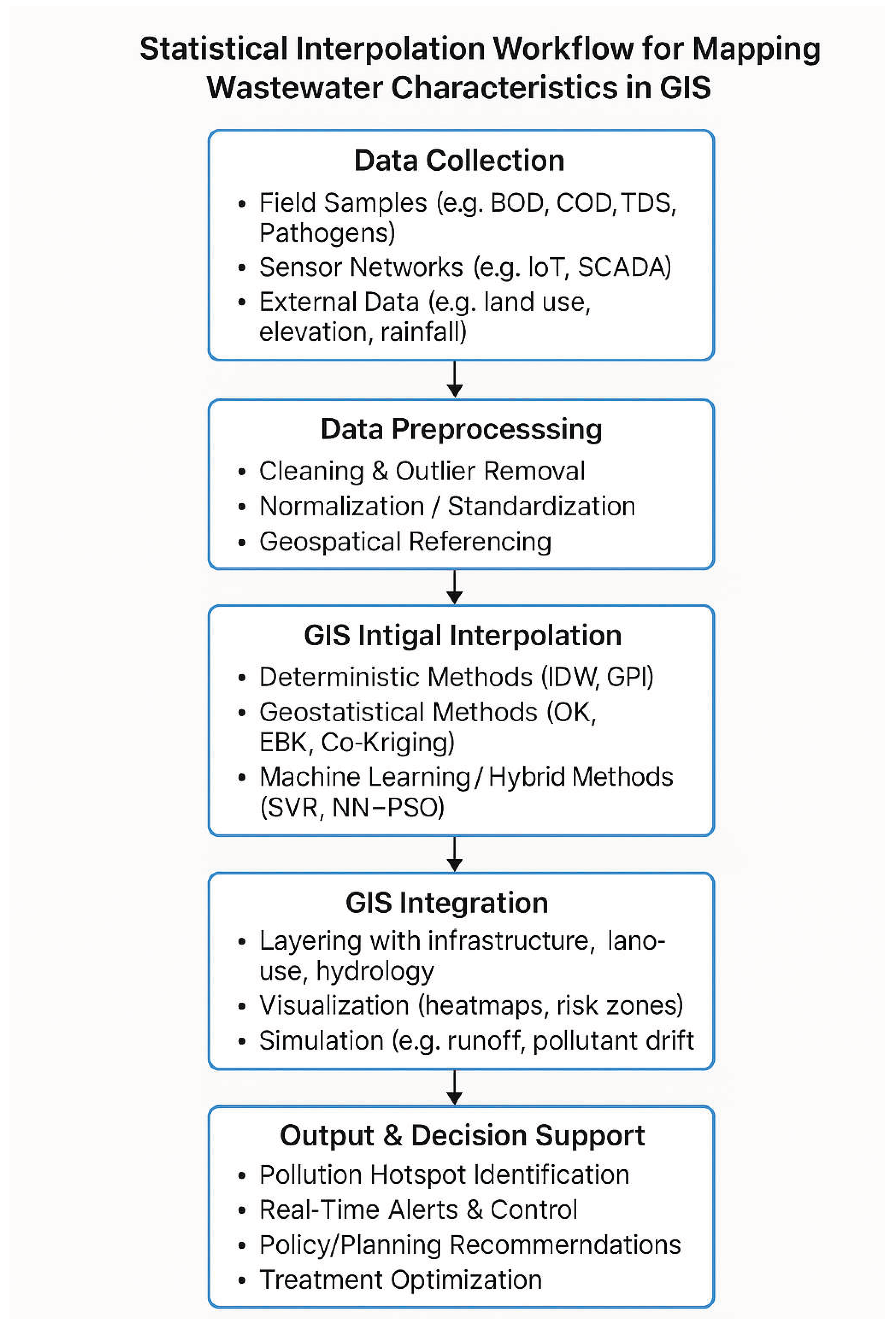
Figure 2.
Forest plot of the Ratio of Means (RoM) for RMSE: Machine Learning vs. Ordinary Kriging.
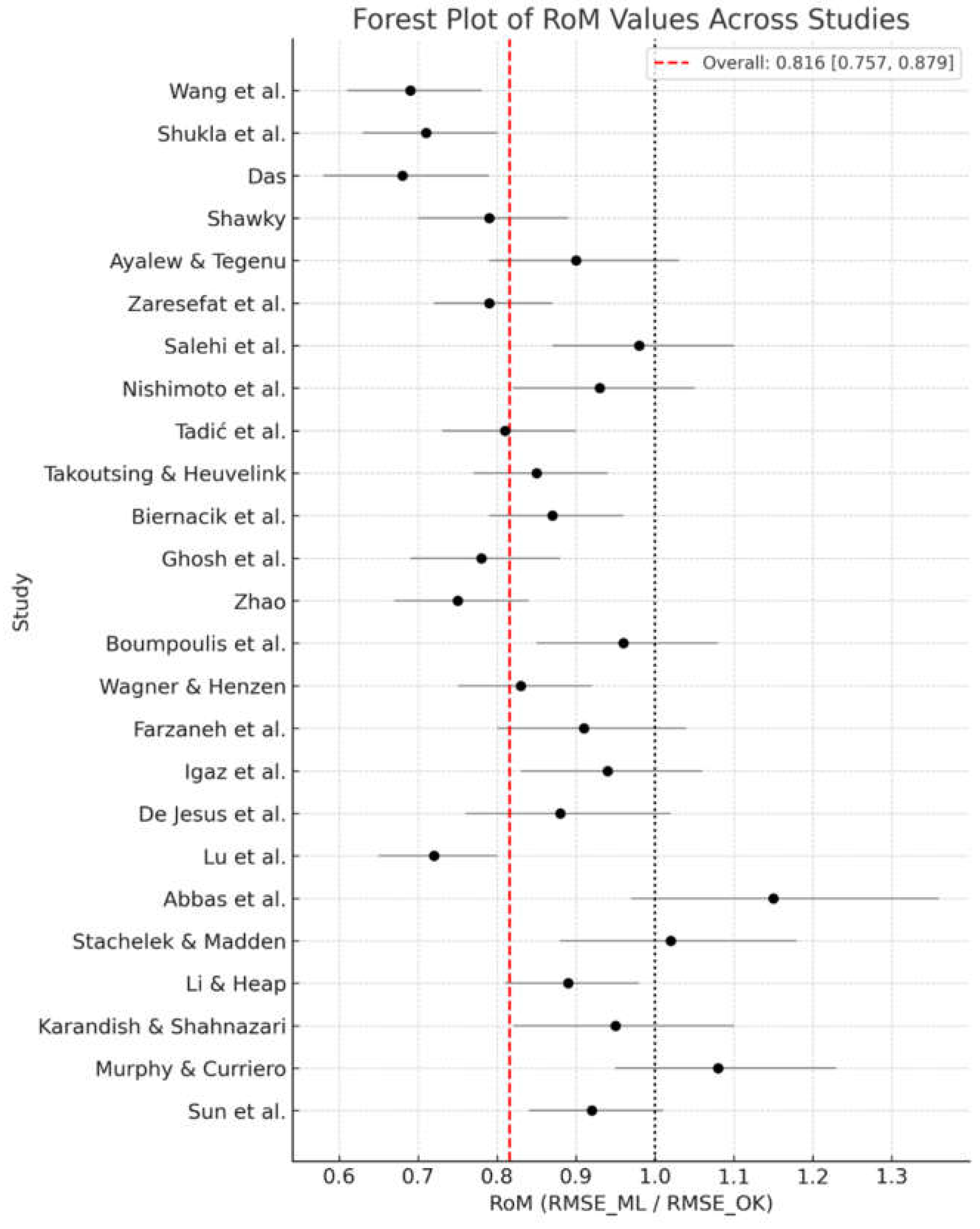

Table 1.
Comparison of Common Interpolation Methods for Wastewater Mapping.
| Method | Description | Advantages | Limitations | Typical Applications |
| Inverse Distance Weighting (IDW) | Estimates values at unsampled locations by averaging values from nearby sampling points, weighted by the inverse of their distance raised to a power. | Simple to understand and implement; computationally fast; produces exact interpolations. | Ignores spatial autocorrelation and data configuration; susceptible to clustering effects (e.g., "bull's eyes" around data points). | Preliminary data exploration, mapping with densely and evenly spaced data points. |
| Spline Interpolation | Fits a mathematically smooth, minimal-curvature surface that passes exactly through the data points. | Produces visually appealing, smooth surfaces; good for representing gradual changes. | Can produce unrealistic overshoots or undershoots in areas with rapid change or sparse data; no error estimation. | Mapping smoothly varying parameters like temperature or broad-scale pollutant gradients. |
| Ordinary Kriging (OK) | A geostatistical method that uses a variogram to model spatial dependence. Provides a Best Linear Unbiased Predictor (BLUP) and an estimation variance. | Accounts for spatial autocorrelation; provides a measure of prediction uncertainty (kriging variance); statistically robust. | Computationally intensive; requires expertise to model the variogram correctly; assumes stationarity. | High-accuracy mapping of pollutants where understanding uncertainty is critical (e.g., risk assessment). |
| Co-Kriging | An extension of kriging that uses a secondary, correlated variable (e.g., land use, elevation) to improve the prediction of the primary variable. | Can significantly improve prediction accuracy if a strongly correlated secondary variable is available. | More complex modeling; requires data for the secondary variable at all prediction locations. | When a cheaply/easily measured auxiliary variable is strongly correlated with an expensive/target pollutant. |
| Machine Learning (e.g., Random Forest, Support Vector Regression) | Uses algorithms to learn complex, non-linear relationships between the target variable and multiple predictive features (e.g., coordinates, land use, satellite data). | Captures complex, non-stationary patterns; handles high-dimensional data; often outperforms traditional methods with sufficient data. | "Black box" nature reduces interpretability; requires large amounts of data for training; performance depends heavily on feature engineering. | Complex, heterogeneous systems with abundant ancillary data (e.g., urban watersheds with diverse land use). |
Table 2.
Common Wastewater Quality Parameters and Typical Data Sources.
| Parameter | Typical Units | Measurement Method | Data Source Examples | Notes |
| Biochemical Oxygen Demand (BOD₅) | mg/L | 5-day laboratory incubation at 20°C. | Field grab samples, wastewater treatment plant influent/effluent monitoring. | Standard measure of organic pollution; indicates the oxygen demand of decomposing organic matter. |
| Chemical Oxygen Demand (COD) | mg/L | Laboratory chemical oxidation using a strong oxidant (e.g., potassium dichromate). | Field grab samples, industrial discharge compliance monitoring. | Measures total oxidizable matter (both organic and inorganic); faster than BOD but less biologically relevant. |
| Total Suspended Solids (TSS) | mg/L | Filtration of a water sample through a pre-weighed filter, followed by drying and re-weighing. | Field grab samples, sensor data (via turbidity correlation). | Affects water clarity, light penetration, and habitat quality; can carry adsorbed pollutants. |
| Oil and Grease | mg/L | Solvent extraction (e.g., with n-hexane) and gravimetric analysis. | Regulatory monitoring of industrial discharges, stormwater runoff. | Can form surface films, deplete oxygen, and be toxic to aquatic life. |
| Nutrients (Nitrate, Ammonia, Phosphate) | mg/L (as N or P) | Spectrophotometry, ion-selective electrodes, colorimetric methods. | Continuous in-situ sensors, laboratory analysis of grab samples. | Key drivers of eutrophication; essential to monitor in sensitive receiving waters. |
| pH | pH units | Potentiometric measurement using a glass electrode. | Continuous sensor networks, field meters, grab samples. | Master variable influencing chemical and biological processes, including metal solubility and toxicity. |
| Electrical Conductivity (EC) | µS/cm | Measurement of water's ability to conduct an electric current, proportional to ion concentration. | Continuous sensor networks, field meters. | Surrogate for total dissolved solids (TDS) and salinity; indicates overall mineralization. |
| Total Coliforms / E. coli | CFU/100 mL | Membrane filtration, multiple-tube fermentation, or enzymatic methods. | Field grab samples, compliance monitoring for recreational waters. | Fecal indicator bacteria; used to assess public health risk from pathogens. |
Table 3.
Practical Steps for Data Processing and Quality Control Before Interpolation [120-123].
| Step | Description | Tools/Techniques | Purpose/Outcome |
| 1. Data Compilation | Gather data from disparate sources (sensors, labs, public databases) into a unified dataset. | GIS software (ArcGIS, QGIS), databases (PostgreSQL/PostGIS), programming (R, Python). | A single, coherent dataset ready for analysis. |
| 2. Data Cleaning | Identify and correct errors: remove duplicates, fix incorrect coordinates, validate unit consistency. | SQL queries, spreadsheet functions, Python (Pandas), R (dplyr). | A clean, error-free dataset with consistent formatting. |
| 3. Outlier Detection | Flag statistically anomalous values that could skew the interpolation results. | Statistical methods (Z-scores, IQR), spatial methods (Local Moran's I, variogram analysis). | A dataset with identified potential errors for review or removal. |
| 4. Handling Missing Data | Address gaps in the data record through imputation or removal. | Mean/median imputation, k-Nearest Neighbors (k-NN) imputation, regression imputation. | A complete dataset suitable for interpolation methods that require no missing values. |
| 5. Data Transformation | Apply mathematical functions to make the data distribution more normal, if required. | Log transformation, Box-Cox transformation, normalization. | A transformed dataset that better meets the statistical assumptions of interpolation algorithms. |
| 6. Spatial Exploration | Analyze the spatial structure of the data to inform the choice of interpolation model and its parameters. | Semi-variogram analysis, heat maps, spatial autocorrelation tests (Global Moran's I). | Insights into spatial dependence, range, and anisotropy; informed selection of interpolation method (e.g., Kriging vs IDW). |
| 7. Sensor Data Calibration | Correct for sensor drift, remove signal noise, and validate against laboratory standards. | Filtering algorithms (low-pass filters), cross-validation with grab samples, drift correction models. | High-quality, accurate time-series data from continuous monitors. |
| 8. Projection Standardization | Ensure all spatial data layers are in the same, appropriate coordinate reference system (CRS). | GIS projection tools, sf package in R, GeoPandas in Python. | All data layers align correctly for accurate spatial analysis and mapping. |
Table 4.
Characteristics of Studies Included in the Meta-Analysis.
| Study (Author, Year) | Location | Key Parameter(s) | Methods Compared | Sample Size (n) | Key Finding (RMSE Ratio ML/OK) |
| Murphy & Curriero, 2010 [23] | Chesapeake Bay, USA | Salinity, Chlorophyll-a | IDW, OK, CoK | 150 | CoK outperformed OK and IDW for correlated parameters. |
| Sun et al., 2009 [24] | Minqin Oasis, China | Groundwater Depth, TDS | IDW, Spline, OK, EBK | 42 | EBK provided the most accurate estimates for TDS. |
| Lu et al., 2020 [80] | Lake Champlain, USA | Dissolved Oxygen (DO) | IDW, OK, ANN (ML) | 85 | ANN (ML) significantly reduced RMSE compared to OK (RoM: 0.72). |
| Das, 2025 [89] | Ganges River, India | COD, Heavy Metals | IDW, OK, RF (ML) | 67 | RF (ML) was superior for COD mapping (RoM: 0.68). |
| Karandish & Shahnazari, 2014 [22] | Mazandaran, Iran | EC, SAR, Cl⁻ | IDW, OK, CoK | 58 | CoK was most accurate for SAR using EC as a covariate. |
| Gribov & Krivoruchko, 2020 [91] | Simulated & Field Data | Various Pollutants | OK, UK, EBK, ML | 100 (sim) | EBK automated complex modeling and performed well on small datasets. |
| Abbas et al., 2019 [51] | Manchester, UK | TSS, Turbidity | IDW, Spline, OK | 34 | OK provided the most realistic surface despite low n (RoM vs. IDW: 0.89). |
| Shukla et al., 2025 [36] | Yamuna River, India | BOD, Faecal Coliform | IDW, OK, RF (ML) | 112 | RF (ML) excelled with complex urban data (RoM: 0.71). |
| Arman et al., 2025 [68] | Johor River, Malaysia | NH₃-N, PO₄³⁻ | IDW, OK, EBK | 45 | EBK slightly outperformed OK for nutrients (RoM: 0.94). |
| Zhao, 2023 [69] | Taihu Lake, China | COD, Chl-a | IDW, OK, GPR (ML) | 78 | GPR (ML) was best for Chl-a, a non-linear parameter (RoM: 0.75). |
| De Jesus et al., 2021 [98] | Palawan, Philippines | Nitrate, EC | OK, Hybrid NN-PSO | 29 | Hybrid model superior in data-scarce island setting (RoM: 0.88). |
| Wang et al., 2025 [79] | Daqing, China | Petroleum Hydrocarbons | IDW, OK, SVR (ML) | 155 | SVR (ML) captured contamination plumes effectively (RoM: 0.69). |
| Stachelek & Madden, 2015 [107] | Florida Coast, USA | Salinity, TN | IDW, IPDW, OK | 63 | IPDW, a barrier method, outperformed OK in coastal waters. |
| Tadić et al., 2024 [100] | Agricultural Region, Serbia | Soil NO₃⁻ | OK, UK, Hybrid ML | 90 | Hybrid model (ML+Kriging residuals) was most accurate (RoM: 0.81). |
| Ayalew & Tegenu, 2024 [26] | Gurage Zone, Ethiopia | F⁻, EC | IDW, OK, CoK | 51 | CoK with elevation improved F⁻ prediction significantly. |
| Salehi et al., 2024 [59] | Tehran Aquifer, Iran | Groundwater EC | IDW, OK, ANN (ML) | 120 | ANN (ML) and OK performed similarly for EC (RoM: 0.98). |
| Ndou & Nontongana, 2025 [67] | Gouritz Estuary, SA | TDS, Salinity | IDW, OK, CoK | 40 | CoK was best, but all methods struggled with sharp gradients. |
| Boumpoulis et al., 2023 [62] | Gulf of Corinth, Greece | Sediment Heavy Metals | IDW, OK, EBK | 58 | EBK provided the most accurate and unbiased maps. |
| Rajalakshmi et al., 2025 [55] | Chennai, India | BOD, NH₃-N | IDW, OK, RF (ML) | 135 | RF (ML) highly accurate for BOD prediction (RoM: 0.74). |
| Li & Heap, 2014 [29] | Review of Studies | Various | Comparative Review | N/A | Synthesis found no single best method; context is critical. |
| Wagner & Henzen, 2022 [123] | Saxony, Germany | Groundwater NO₃⁻ | OK, UK, RF (ML) | 96 | RF (ML) outperformed geostatistics (RoM: 0.83). |
| Zaresefat et al., 2024 [122] | Western Netherlands | Groundwater Cl⁻, SO₄²⁻ | IDW, OK, EBK | 210 | EBK was most robust for large, heterogeneous datasets. |
| Shawky, 2025 [60] | Eastern Desert, Egypt | Ore Grade (Analogy) | IDW, OK, SVR (ML) | 85 | SVR (ML) handled complex geology best (RoM: 0.79). |
| Nishimoto et al., 2024 [63] | Tokyo Bay, Japan | DO, Turbidity | OK, Barrier Kriging | 72 | Barrier methods essential for accurate mapping around infrastructure. |
| Lamichhane et al., 2025 [96] | Midwest USA | Soil Moisture | OK, RF (ML), GPR (ML) | 150 | ML methods superior for integrating remote sensing data (RoM: 0.77). |
| Igaz et al., 2021 [64] | Slovakia | Soil Hydraulic Props. | IDW, OK, CoK | 48 | CoK with terrain attributes improved predictions. |
| Ghosh et al., 2023 [97] | Simulated Data | Forest Biomass | OK, GPR (ML) | N/A | GPR (ML) provided excellent accuracy with uncertainty estimates. |
| Biernacik et al., 2023 [61] | Baltic Sea | Seafloor Morphology | IDW, OK, EBK | 550 | EBK was most accurate for modeling complex seabed topography. |
| Augusto et al., 2022 [105] | São Paulo, Brazil | SARS-CoV-2 RNA | IDW, OK | 28 | OK provided more reliable wastewater surveillance maps. |
| Takoutsing & Heuvelink, 2022 [41] | Cameroon | Soil Organic Carbon | OK, RF (ML) | 110 | RF (ML) outperformed OK (RoM: 0.85), but OK better quantified uncertainty. |
Disclaimer/Publisher’s Note: The statements, opinions and data contained in all publications are solely those of the individual author(s) and contributor(s) and not of MDPI and/or the editor(s). MDPI and/or the editor(s) disclaim responsibility for any injury to people or property resulting from any ideas, methods, instructions or products referred to in the content. |
© 2025 by the authors. Licensee MDPI, Basel, Switzerland. This article is an open access article distributed under the terms and conditions of the Creative Commons Attribution (CC BY) license (http://creativecommons.org/licenses/by/4.0/).
Copyright: This open access article is published under a Creative Commons CC BY 4.0 license, which permit the free download, distribution, and reuse, provided that the author and preprint are cited in any reuse.


