Submitted:
24 November 2025
Posted:
25 November 2025
You are already at the latest version
Abstract
In the macro context of promoting sustainable development and achieving net zero emissions, the role of green technology innovation, renewable energy utilization and environmental policy is crucial. Based on the panel data of 35 OECD economies from 1990 to 2019, this study adopts the augmented mean group (AMG) as the main estimation method, and uses the common correlation mean group (CCEMG) for robustness test, and tests the causal relationship between variables through Dumitrescu-Hurlin method. The results show that both GTI and renewable energy consumption have a significant positive impact on CO 2 emission reduction. Environmental taxes are positively correlated with carbon emissions, but not statistically significant, and the CCEMG estimation results are consistent with AMG. The causality test further reveals that there is a significant bidirectional causality among the variables. Therefore, it is recommended that OECD countries give priority to expanding investment in green technologies and renewable energy infrastructure, and re-evaluate and optimize environmental tax policies to effectively promote the transition to a low carbon economy.
Keywords:
green technology innovation
; renewable energy consumption
; environmental tax
; net-zero emissions
; sustainable development
; OECD countries
1. Introduction
IPCC (2023) urgency necessitates OECD economies reconcile growth with environmental sustainability through three key strategies. Green technology innovation advances energy efficiency but faces adoption barriers (Zeng et al., 2024)[1]. Renewables like solar/wind are now cost-competitive and reduce carbon intensity (IRENA, 2022)[2], yet require policy-enabled infrastructure integration and just transitions for fossil-dependent communities (Hassan et al., 2024a; Shobande et al., 2025)[3,4]. Environmental taxes internalize CO2 costs (Zhu et al., 2023)[5], but exhibit variable efficacy, demanding optimal design—calibrated rates, revenue recycling, and competitiveness safeguards—to drive emission-reduction cycles. (OECD, 2021)[6].
Despite OECD countries’ disproportionate share of global emissions (Figure 1 and Figure 2) and binding climate commitments, empirical analyses examining the integrated impact of these three drivers remain underrepresented. This study addresses this critical gap by investigating how green innovation, renewable consumption, and environmental taxes collectively reduce CO2 emissions and advance sustainability objectives across 35 OECD economies (1990–2019). Employing advanced second-generation econometric techniques—specifically the Augmented Mean Group (AMG) estimator with Common Correlated Effects Mean Group (CCEMG) robustness checks—the methodology overcomes limitations of cross-sectional dependence and heterogeneity that compromised prior studies, enhancing result generalizability.
Green innovation and renewable energy significantly mitigate CO2 emissions, providing actionable pathways to reconcile economic growth with environmental goals. Conversely, environmental taxes exhibit a positive but statistically insignificant relationship with emissions, indicating current designs fail to deter pollution—necessitating context-sensitive reforms over uniform approaches. These robustly validated results align with UN SDGs: renewables advance SDG 7; green innovation supports SDG 9; tax analysis furthers SDG 12; collectively underpinning climate action.
The global pursuit of sustainable development and the transition to net-zero emissions has become a paramount objective in the face of escalating climate change, environmental degradation, and resource depletion. The IPCC (2023)[7] emphasizes urgent action, prompting OECD countries to align economic growth with environmental sustainability. Key strategies include green technology innovation, renewable energy expansion, and environmental taxation, which have shown significant CO2 emission reductions (Figure 1 and Figure 2).
IRENA (2022) confirms renewables like solar and wind are now among the most economical global power sources. OECD countries have significantly expanded renewable energy shares, reducing carbon intensity (Mahmood et al. 2022)[8]. However, transitioning to fully renewable systems faces integration challenges (Hassan et al., 2024b)[9]. requiring continued technological advancements and policy mechanisms to enable large-scale adoption. Additionally, a just transition for fossil fuel-dependent communities requires targeted emission-mitigation policies aligned with sustainable development and net-zero goals (Shobande et al., 2025)[4].
Consequently, OECD policymakers must prioritize scaling green R&D investments and renewable infrastructure while redesigning environmental tax frameworks with revenue recycling. This integrated approach provides methodologically robust decarbonization evidence for advanced economies. The paper proceeds as follows: Section 2 reviews extant literature, Section 3 details data and methodology, Section 4 presents and analyzes results, and Section 5 concludes with policy implications.
2. Review of literature
2.1. Green Technology Innovation and CO2 Emissions
The relationship between green technology innovation (GTI) and CO2 emissions is critical for climate mitigation. While most research indicates GTI reduces emissions, significant nuances and contextual dependencies exist. Empirical studies across jurisdictions confirm GTI’s generally negative association with emissions.Popp (2019)[10] demonstrates this in OECD nations using patent data as an innovation proxy. Cross-country analyses by Dechezleprêtre et al. (2011)[11] and Aghion et al. (2019)[12] further establish that economies with higher green patent filings exhibit slower CO2 growth and lower per capita emissions. Regional studies reinforce this: Zhou et al. (2024)[13] find GTI reduces emissions in Europe. Liu et al. (2025)[14] highlight GTI’s enhanced effectiveness in Chinese regions with stringent environmental regulations. However, counterintuitive findings reveal limitations. Obobisa and Ahakwa (2024)[15] document increased CO2 emissions post-GTI adoption in some European contexts, suggesting potential rebound effects where efficiency gains spur higher consumption. Lambrecht and Willeke (2025)[16] demonstrate this paradox in transportation: while per-unit emissions fall, total emissions rise due to increased vehicle usage.
2.2. Renewable Energy Consumption and CO2 Emissions
Renewable energy is pivotal for decarbonization and achieving net-zero targets, directly advancing SDGs 7 and 13 (Cao et al., 2025; Paraschiv and Paraschiv 2023)[17,18]. By displacing fossil fuels, it enhances energy security, stimulates sustainable growth, and reduces CO2 emissions (Han et al., 2025)[19]. Empirical evidence confirms this inverse relationship across OECD countries (Obobisa, 2024)[20], and the U.S., where renewables underpin carbon neutrality (Yuan et al., 2022)[21]. Stronger effects in low-emission economies (Wolde-Rufael & Mulat-Weldemeskel, 2022)[22]. However, rebound effects stimulate higher consumption from efficiency gains (Saunders, 2013)[23]. Consequently, marginal decarbonization can be modest—York (2012)[24] documents just a 0.1% decrease per 1% renewable penetration increase. Thus, while fundamental to climate strategies, renewables’ net environmental benefit depends critically on overcoming intermittency through storage, implementing demand-side policies to counter rebound effects, ensuring sustainable supply chains, and adapting to national contexts.
2.3. Environmental Tax and CO2 Emissions
Environmental taxes (ETAX), including carbon levies, internalize pollution’s social costs to incentivize cleaner energy use. Empirical research generally supports their efficacy in reducing CO2 emissions and accelerating renewable adoption, as demonstrated by meta-analyses (Ahmad et al., 2024)[25], cross-national studies (Shahbaz et al., 2020; Doğan et al., 2022)[26,27], and successful implementations like Sweden’s carbon tax achieving 25% emission reductions alongside growth (Andersson, 2019)[28]. However, effectiveness is contingent on three design elements: appropriate tax rates reflecting environmental damage, revenue recycling to fund green investments or household compensation, and complementary policies (Goulder and Hafstead, 2017)[29]. Notably, paradoxical outcomes emerge in weak enforcement regimes where taxes trigger fossil fuel smuggling (Alola et al., 2023)[30] , highlighting critical context dependencies.
2.4. Gap in Literature
Conventional research inadequately addresses cross-sectional dependence/heterogeneity and underrepresents integrated analyses of green innovation, renewables, and environmental taxes in OECD economies despite their global emissions significance. This study addresses these gaps by empirically examining these factors’ collective impact on carbon neutrality across 35 OECD countries using second-generation econometric techniques to overcome methodological constraints.
3. Materials and Methods
3.1. Theoretical Rationale and Empirical Model Building
This study integrates interdisciplinary theories—technological change for environmental efficiency, energy transition, and Pigouvian taxation—to analyze how green innovation, renewable energy, and environmental taxes collectively reduce CO2 emissions. Concurrently, energy transition theory emphasizes fossil fuel displacement by renewables as critical for climate mitigation and achieving SDGs 7 and 13 (Adams & Acheampong, 2019)[31]. Pigouvian tax theory contends that environmental taxes internalize pollution costs by incentivizing cleaner practices and generating revenue for reinvestment in green technologies, creating an innovation-emission reduction cycle (Qiu et al., 2020)[32].
Considering the afore-discussed theoretical foundations, this extant study proposed a panel model in a multivariate framework to estimate the impact of green technological innovation, renewable energy consumption, and environmental taxes on CO2 emissions in OECD economies. Importantly, the explanatory variables must be written as a linear combination of their associated parameters for estimation purposes. Hitherto, data pertaining to all the variables have been converted to natural logarithms in order to reduce heteroscedasticity concerns. Thus, our proposed transformed log-linear model in a panel multivariate context is specified as;
where lnCO2, lnGTI, lnREC, and lnETAX, respectively, represent the natural logarithm transformations of carbon dioxide emissions, green technological innovation, renewable energy consumption, and environmental tax, is the error term, while and indicate the country cross sections and time.
In particular, to control for socioeconomic conditions in nations and time-varying bias that may influence changes in the dependent variable, the study incorporated control variables such as income and government health spending. Thus, the specified model in Equation (2) is extended as;
where is a constant term for the individual cross-sections, , and are the parameter estimates of capturing the effect of green technological innovation, renewable energy consumption and environmental tax correspondingly, is vector of parameters that accounts for the respective effect of the control variables, whereas is also a vector containing the control variables (economic growth (GDP) and fossil fuel energy consumption (FEC)), where and represent individual countries within a panel at a specific time correspondingly and represents the error term.
Controlling for GDP and fossil fuel consumption is essential to isolate the impact of green policies on CO2 emissions, as their confounding effects distort findings. GDP fluctuations conflate cyclical economic effects with policy outcomes—expansions elevate emissions despite green advancements, while downturns create false positives. Omitting fossil fuel consumption risks misattributing reductions to renewables rather than market-driven fossil volatility, inducing omitted variable bias given energy system interdependencies (Apergis & Payne, 2010)[33]. Environmental tax efficacy further depends on economic/energy contexts (Metcalf, 2009)[34], while rebound effects necessitate GDP controls to quantify green innovation’s net impact. Fossil fuel controls prevent overstatement of renewables’ displacement effects (Stern, 2017)[35], collectively mitigating biases and clarifying decarbonization pathways.
3.2. Estimation Approach
Prior to estimating the effect of environmental tax, renewable energy consumption, and green technological innovation on CO2 emissions whilst controlling for economic growth and fossil fuel energy consumption, the following standard panel econometric procedures are carried out steadily. First, the existence of cross-section CSD is examined. CSD arises when unobserved common factors such as global economic shocks, shared policies, or spatial spillovers induce correlations in residual across units (countries), violating independence assumptions. Ignoring this can lead to biased standard errors and invalid inferences. Based on this, the Pesaran CSD (PCSD) test by Pesaran (2004)[36] is employed to examine the issues relating to cross-sectional dependence. The test statistic of the PSCD test is derived from the pairwise correlation coefficients of residuals obtained from individual regressions for each cross-sectional unit. Specifically, for a panel with cross-sectional units and periods, the PCSD test calculates the average of all pairwise correlation of residuals between units and (denoted as ), then standardizes this average to form a statistic that asymptotically follows the standard normal distribution under the null hypothesis of no cross-sectional dependence. The test equation is formulated as;
where is the sample of the correlation coefficient between the residuals of the units and . Under the null hypothesis of cross-sectional independence, CSD converges to a normal distribution with mean 0 and variance 1. A significant PCSD test value rejects the null hypothesis, indicating the presence of cross-sectional dependence.
Bearing in mind the potential existence of cross-sectional dependence in panel data settings, it would not be econometrically meaningful to use conventional unit root tests such as the ADF test, PP test and IPS test, since they do not produce robust and reliable outcomes in the presence of cross-sectional dependence issues. In line with this, the study employed a second generation unit root test by Pesaran (2008)[36] known as the cross-section Im, Pesaran and Shin (CIPS) test, in the second phase of the estimations procedure to examine the stationarity properties of the study variables. The CIPS explicitly models dependence by augmenting the standard Dickey-Fuller (DF) regressions with cross-sectional averages of lagged levels and the first differences of the series. For a panel dataset with cross-sectional units (countries) and time periods, the CIPS test estimates the cross-sectional augmented DF regression for each unit :
where is the first difference of the variable , is the lagged level of , is the cross-sectional average of lagged first differences, is the cross-sectional difference of the lagged levels, whereas , and are unit-specific coefficients. The inclusion of and accounts for common factors affecting all units, mitigating cross-sectional dependence. The CIPS statistic is thus estimated as the cross-sectional averages of the statistics () for the null hypothesis of (unit root exist) from ach cross-section augmented DF regression:
Having confirmed the integration order of the utilized variables, the study further examined the existence of cointegration or long-run liaison among variables within the proposed empirical model using the Westerlund(2007)[37] (WE) cointegration test. The test employs an error correction model framework. Thus, for a panel with cross-section units and time periods, the error correction model for unit is specified as:
where captures the cointegration relationship (speed of adjustment towards the long-run equilibrium) with being the lagged dependent variable, the lagged independent variable(s), the vector of cointegration coefficients, represents the lags of the dependent variable’s first difference, capturing the short-term effect and denotes the lags of the independent variable(s)’s first difference, capturing the short-term dynamics of ’s. The test computes four statistics: two group-mean statistics ( and ), which explores the alternate theory of cointegration of the whole group and two-panel statistics ( and ), which, on the other hand, notes that at least one cross-section of the panel is cointegrated. The group-mean statistics aggregate individual unit results, with averaging the statistics of and averages normalized adjustment speeds as:
where is the standard error of . The panel statistics pools data across units, with and derived from pooled estimates of as:
The WE cointegration test relies on the null hypothesis, , which posits no cointegration across units, while the alternative , suggests cointegration in at least one unit. Critical values are generated via a sieve bootstrap procedure to address cross-sectional dependence. This method resamples residuals while preserving their cross-unit correlation structure, ensuring robustness to shared trends or shocks.
Further, heterogeneity -where parameters vary across cross-sectional units -reflects divergent responses to variables due to institutional, cultural or economic differences. Specifically, the presence or absence of slope heterogeneity leads to the selection of an appropriate estimator for estimating the slope coefficients with respect to the variables specified in the study’s proposed model. Thus, to determine whether slope heterogeneity is an issue of concern,the Pesaran and Yamagata (2008)[36] (PY) test is employed prior to finally estimating the relationship among the study variables. The PY test extends Swamy’s method by addressing small-sample bias and cross-sectional dependence. Under the null hypothesis , slope coefficients are identical across units (homogeneity), while the alternative allows heterogeneity (). The test employs two test statistics, which include the delta tilde () and adjusted delta tilde () which modify the Swamy’s statistic to correct for bias in finite samples. The statistics are thus estimated as follows;
where represent the unit-specific ordinary least square estimates, is a weighted fixed-effects pooled estimator, is the matrix of regressors, is the within-group matrix, is the error variance estimate for unit , is the number of regressors, and are cross-sectional and time dimensions, and is the Swamy’s original statistic. Under the null hypothesis, and converge to a standard normal distribution for large and . Rejection of the null hypothesis thus implies slope heterogeneity, necessitating the implementation of estimators like the AMG, CCEMG, just to mention a few.
Addressing cross-sectional dependence and slope heterogeneity, this study estimates cointegration between CO2 emissions, environmental taxes, and renewable energy—controlling for GDP and fossil fuels—using AMG (Bond & Eberhardt, 2013)[38] and CCEMG (Pesaran, 2006)[39]. Unlike traditional FE/GMM methods imposing homogeneity assumptions, AMG incorporates common dynamic effects (θₜ) capturing unobserved time-varying factors across units, thereby correcting for heterogeneity biases while averaging unit-specific coefficients. This approach ensures robust estimation where conventional methods fail.The AMG model for unit at time is thus expressed as:
where is the dependent variable, is a vector of independent variables, is a unit-specific intercept, represents unit-specific slopes, and is a common term (often proxied by the cross-sectional average of or time dummies). By specifying or reformulating the Equation (10) with the study variables, the AMG model to be estimated in this study thus becomes;
From Equation (11), the AMG estimates for the coefficients or parameters with respect to the explanatory variables and control variables are thus determined by using the cross-sectional means of ’s and ’s as follows:
where and are the AMG estimators of the explanatory variables of interest and control variables for each cross-sectional unit in the panel, and are the parameter estimates concerning the explanatory variables of interest and the control variables utilized in this study.
On the other hand, the CCEMG estimation method accounts for cross-sectional dependence by including cross-sectional averages of the dependent and independent variables as proxies for unobserved common factors. Using the cross-section averages of the regressors together with that of the response variable, the CCEMG approach approximates latent common factors, allowing the model to filter out cross-unit correlations. Thus, for a cross-sectional unit at time , the CCEMG model is theoretically expressed as;
where and are the cross-sectional averages of the response and regressors at time , whereas and respectively denotes specific unit coefficients of the cross-sectional means of the response and explanatory variables. By specifying the theoretical model in Equation (14) with the study variables, the CCEMG model is empirically expressed as:
where , , , and represents the cross-sectional averages , , and together with the control variables and is the slope coefficient of the control variable.
Similar to the AGM estimator, the CCEMG estimates for the coefficients or parameters with respect to the explanatory variables and control variables are thus determined by the following relations;
where and are the CCEMG estimators for the explanatory variables and control variables for each cross-sectional unit in the panel, and are the parameter estimates concerning the explanatory variables of interest and the control variables utilized in this study.
Since the recommended estimation approaches (AMG and CCEMG) only give elasticity inference, the direction of causal relationships between the employed study variables is examined by employing the panel causality approach of Dumitrescu and Hurlin (2012)[40] (henceforth, DH-test). Unlike conventional tests assuming homogeneous causality, the DH test explicitly accommodates heterogeneity—allowing causal relationships to exist in some cross-sectional units but not others—making it ideal for contexts where structural or institutional differences cause varying effects across economies. The test implements a panel vector autoregressive (VAR) framework to determine if lagged values of variable X improve predictions of variable Y beyond Y’s own history, thereby robustly identifying causal pathways amid unit-specific variations.Thus, for each cross-section unit and time , the model is specified as;
where represents unit-specific fixed effects, and are the lag coefficients specific to unit and is the error term. The null hypothesis posits that does not Granger-cause in any unit , while the alternative hypothesis allows for causality in at least some units . This formulation explicitly acknowledges heterogeneity as a causal effect () are permitted to differ across units. The test statistic is constructed in two stages. First, individual Wald statistics are computed for each unit to test the null hypothesis . These statistics are then averaged across units to form the panel statistic . To address cross-sectional dependence and ensure asymptotic normality, the standardized statistic is derived, where is the number of cross-sectional units, and is the number of lags. Under the null, converges to a standard normal distribution, enabling hypothesis testing.
In summary, the analytical roadmap is pictorially illustrated in Figure 3 as:
3.3. Data and Descriptive Analysis
Based on data availability, this study uses annual data of 35 OECD economies from 1990 to 2019. Data on green technology innovation and environmental taxes were sourced from the OECD statistics database. Renewable energy consumption, fossil fuel energy consumption, and GDP were sourced from the World Development Indicators (WDI). The selected variables are based on the United Nations Sustainable Development Goals (7, 8, 9, and 13). Table 1 contains definitions of the variables and data sources.
Table 2 summarizes descriptive statistics for the study variables using their respective means, median, maximum and minimum values, standard deviations, skewness and kurtosis, Jarque-Bera test, and Variance Inflation Factor (VIF) outcomes. The descriptive statistics, as outlined in Table 2, provide insights into the distribution and characteristics of the study variables. Specifically, the mean values indicate the average level of each variable across 1,050 observations, with CO2 emissions averaging 11.531, GTI AT 4.168, REC at 2.375, ETAX at 0.766, FEC at 4.248, and GDDP at 10.111. The median values, which are close to their respective means, on the other hand, suggest a relatively symmetrical distribution of more variables. Further, the maximum and minimum values highlight the range of variation within the dataset. Evidently, CO2 emissions range from 7.528 to 15.569, GTI varies significantly from -1.722 to 9.429, and ETAX shows a particularly large spread from –4.200 to 1.681, indicating substantial differences in environmental tax policies. The standard deviation values also suggest the extent of variability in each variable, with GTI exhibiting relatively higher variability at 2.380, while ETAX and FEC show lower dispersion at estimated values of 0.471 and 0.386, respectively. Overall, the standard deviation suggests that while some variables, such as GTI, have substantial fluctuations, others, like ETAX and FEC, display more stability within the dataset.
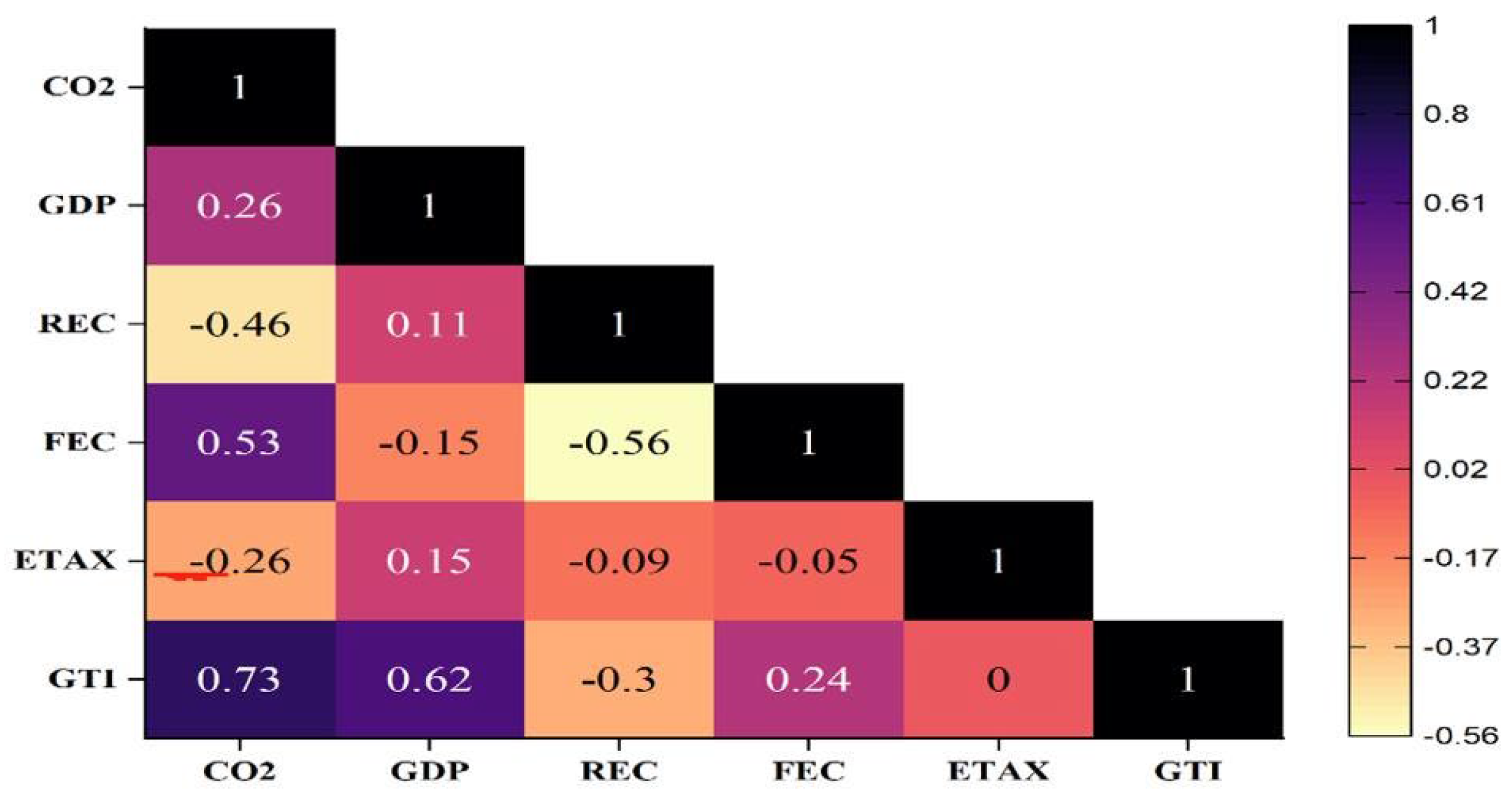
From the side of the skewness and kurtosis, CO2 emissions, GTI, and GDP recorded skewness values near zero, implying near-normal distributions. However, ETAX and FEX exhibit significant negative skewness, indicating longer left tails, meaning that some regions in the OECD community impose substantially lower environmental taxes or have lower fuel energy consumption. REC also shows mild negative skewness, suggesting that more observations lean toward lower renewable energy consumption. Moreover, while CO2 emissions, GTI, REC, and GDP have moderate kurtosis values around 3, indicating near-normal distributions, ETAX and FEC display extremely high kurtosis values, suggesting heavy tails with extreme values in their distributions. The Jarque-Bera test results confirm that all variables except CO2 emissions deviate from normality, as indicated by probability values of 0.000, which reject the null hypothesis of normality. The VIF values finally indicate the level of multicollinearity among the independent variables. All VIF values are evidenced to be below the threshold of 5.0, with ETAX having the lowest at 1.08 and GTI the highest at 2.29. These values suggest that multicollinearity is not an issue of concern in the dataset, ensuring a more reliable regression estimate. The correlation among the explanatory variables from the heat correlation matrix in Figure 6 supports this outcome of the missing issue of multicollinearity.
Moreover, Figure 5 displays a box-violin plots analysis of CO2 emissions, GTI, REC, ETAX, GDP, and FEC. For CO2 emissions, the interquartile range indicates a moderate variability in emission levels, with the median positioned centrally, reflecting balanced dispersion. GTI also exhibits a compact interquartile range, suggesting clustered data around the median, which may imply limited but consistent adoption of sustainable technologies. REC also exhibits a similar narrow spread, highlighting regional similarities in OECD economies’ renewable energy usage, although the median levels may reflect modest overall adaptation. Moreover, ETAX displays a tilted distribution, with the median closer to the lower quartile, indicating that most regions in the OECD economies implement relatively low tax policies. Conversely, FEC has a wide interquartile range, underscoring significant variability in reliance on non-renewable energy sources, with the median indicating a moderate overall dependence. GDP finally demonstrates a right-skewed distribution, where the median is closer to the lower end of the scale, indicating economic disparities, as most nations in the OECD community exhibit lower GDP levels.
Figure 4’s scatter plots reveal critical bivariate relationships: CO2 emissions exhibit a counterintuitive positive correlation with GTI, suggesting innovations may coexist with carbon-intensive processes or exhibit delayed mitigation effects. Conversely, REC shows a clear negative correlation, confirming cleaner energy’s decarbonization role. ETAX displays no discernible trend, indicating effectiveness depends on enforcement rigor, rate calibration, and complementary policies. FEC demonstrates a strong positive relationship, reinforcing carbon-intensive energy’s environmental impact. GDP exhibits a weak positive correlation, with data dispersion reflecting heterogeneous growth-emissions linkages across economies due to varying efficiency and policies. These visual patterns align with Figure 6’s correlation matrix, collectively highlighting the complex, variable-specific dynamics governing emission drivers in OECD nations.
Figure 4.
Scatter plot for the relationship between CO2 emissions and each of the explanatory variables (GTI, REC, ETAX, FEC, and GDP). Figure 4. a CO2 emission with green technology innovation. Figure 4. b CO2 emissions with renewable energy consumption. Figure 4. c CO2 emissions with environmental tax. Figure 4. d CO2 emissions with fossil fuel energy usage. Figure 4. e CO2 emissions with GDP.
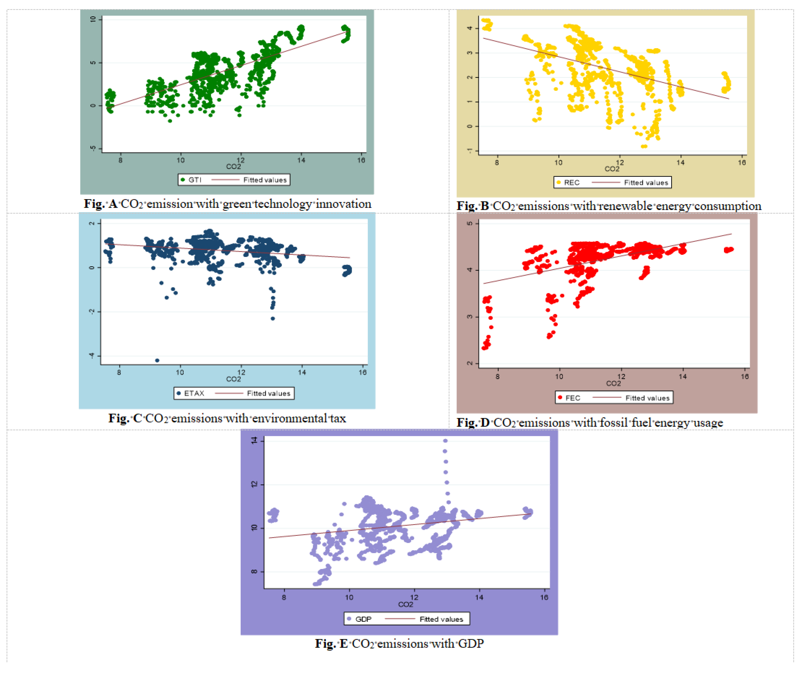
Figure 5.
Boxplot analysis of variables.
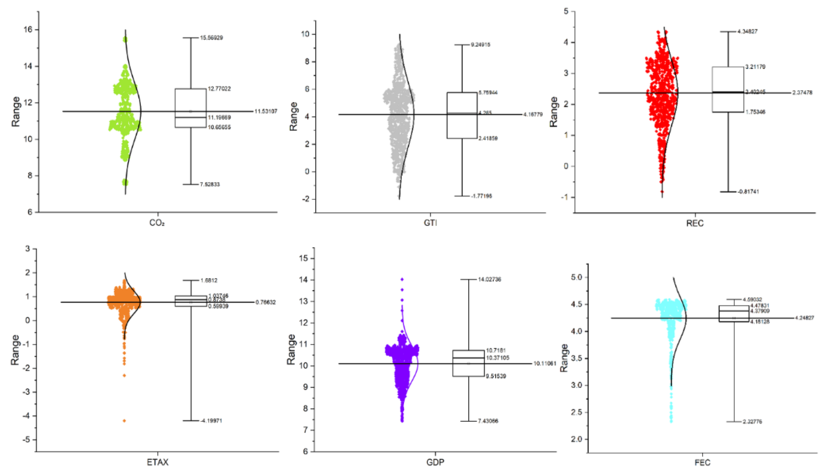
Figure 6.
Correlation matrix.
4. Results and Discussions
4.1. Preliminary Analysis
The results from the Pesaran (2004)[41] PCSD test and the test of slope homogeneity are presented in Table 3.
Specifically, the PCSD test is based on the null hypothesis that there is no residual cross-section correlation across the cross-sections with the panel of OECD economies, as opposed by the alternative hypothesis, which states vice versa. Evidently, the findings from the PCSD test led to the rejection of the null hypothesis since all test values for each utilized variable is statistically significant at 1%. This thus points out the interconnectedness of these economies regarding the study’s variables and further explains why the fight against CO2 emissions requires unanimous action. Further, the slope homogeneity test is evaluated using the delta tilde () and adjusted delta tilde () test statistics of Pesaran and Yamagata, assuming homogenous slopes across cross-sectional units as the null hypothesis. From the results in Table 3, the null hypothesis of slope homogeneity is rejected since the estimated test values for both delta tilde () and adjusted delta tilde () tests are statistically significant. This thus implies that, there slope variability or heterogeneity among variable across the cross-sectional unit with the study’s panel of OECD countries. With the evidence concerning the presence of residual cross-sectional dependence and slope heterogeneity, a conclusion can be drawn that adopting conventional unit root tests and cointegration methods could render the conclusions biased.
Addressing cross-sectional dependence and slope heterogeneity, this study employs the CIPS unit root test (Table 4), confirming all variables are integrated of order one [I(1)]—non-stationary at levels but stationary when first-differenced. This common integration order (Saud et al. 2019)[42] enables cointegration testing. The Westerlund-Edgerton approach (selected for robustness to cross-dependence per Dauda et al., 2021)[43] rejects the null hypothesis of no cointegration across all four statistics (, , and ) in Table 5. This provides robust evidence of a significant long-run equilibrium relationship among variables, warranting subsequent estimation of cointegrating vectors.
4.2. Long Run Estimation Results
Addressing cross-sectional dependence and slope heterogeneity, this study employs the AMG estimator (with CCEMG robustness checks) to quantify long-run elasticities. Table 6 thus displays the long-run findings for AMG and CCEMG estimators. Results confirm green technology innovation significantly reduces CO2 emissions, with a 1% increase yielding a 0.019% decrease. While this marginal effect appears modest relative to Paris Agreement targets requiring 40-50% reductions, it demonstrates innovation’s cumulative decarbonization potential when scaled. Crucially, achieving deep emissions cuts necessitates integrating green innovation within a broader policy mix—including accelerated renewable adoption, strengthened environmental taxation, and enhanced energy efficiency—rather than relying on incremental technological advances alone.
The significant negative coefficient for green technological innovation confirms its efficacy in mitigating CO2 emissions across OECD economies. This outcome reflects stringent environmental policies—subsidies, tax incentives, and emissions standards—that incentivize firms to adopt innovations, creating a positive feedback loop enhancing sustainability. Similarly, renewable energy consumption exhibits a statistically significant adverse relationship with emissions: AMG estimations indicate a 0.210% emissions reduction per 1% renewable increase. This demonstrates renewables’ capacity to displace fossil fuels within OECD energy matrices, particularly where supportive regulatory frameworks enhance economic viability. The transition bolsters energy security through supply diversification while aligning with net-zero objectives, corroborating studies emphasizing renewables as prerequisites for carbon neutrality (Bistline & Blanford, 2021; Mujtaba et al. 2022; Obobisa 2023)[44,45,46]. Critically, these findings underscore that technological advancement and renewable deployment—reinforced by policy mechanisms—collectively drive emission reductions in advanced economies. Consequently, OECD nations must prioritize scaling R&D investments in green technologies and expanding renewable infrastructure to accelerate decarbonization.
Regression analysis shows a statistically insignificant positive relationship between environmental taxes and CO2 emissions in OECD countries, where a 1% tax increase correlates with a 0.033% emissions rise. This paradox suggests current tax designs fail due to suboptimal rates, extensive exemptions, and weak enforcement, allowing cost-passing rather than green innovation. Sectoral resistance and Ayin and Esen’s threshold theory indicate taxes only reduce emissions above critical behavioral-change levels, implying OECD rates are sub-threshold. Effective decarbonization requires recalibrating taxes with fewer exemptions, higher thresholds, and strategic revenue recycling, consistent with prior studies.
Regression analysis confirms robust positive relationships: a 1% GDP increase elevates CO2 emissions by 0.404% (AMG), reflecting industrialization’s scale effects that amplify fossil fuel demand despite efficiency gains. Fossil fuel consumption shows an even stronger impact (0.835% emissions rise per 1% increase), underscoring thermodynamic realities and OECD’s structural carbon dependency. These persistent linkages—aligning with environmental Kuznets curve dynamics (Ganda, 2019a; Hashmi & Alam, 2019; Wang et al., 2020)[47,48,49]—reveal decarbonization efforts are insufficient to offset growth-driven emissions momentum. OECD nations must therefore accelerate structural transitions via aggressive renewable integration, fossil subsidy reallocation, and systemic innovations to disrupt the entrenched growth-emissions trajectory and achieve meaningful decoupling.
OECD economies’ persistent fossil fuel dependence demonstrably elevates CO2 emissions, validating established ecological impacts and aligning with prior findings (Obobisa, 2022)[50]. Summarily, the graphic of the long-term results is shown in Figure 7.
Methodologically, the AMG estimator’s robustness was confirmed through Wald tests indicating strong predictive validity and cross-validated via CCEMG estimation. Although coefficient weights varied slightly(Ref. second column of Table 6), both approaches produced consistent directional results—attributable to their shared capacity for addressing cross-sectional dependence and heterogeneity through distinct factor modeling (AMG directly estimates common factors; CCEMG incorporates cross-sectional averages). This methodological convergence underscores the reliability of the emissions drivers identified in our analysis.
4.3. Causality Test
Table 7’s panel causality test reveals bidirectional causation between CO2 emissions and key explanatory variables—green technology, renewables, environmental taxes, fossil fuels, and GDP—in OECD countries. This highlights a complex, interdependent system where economic, technological, and policy factors both drive and are driven by carbon emissions. Such feedback loops mean progress in one area can lower emissions, yet persistent emissions or slow transitions can hinder decarbonization efforts and reinforce emissions, complicating the energy transition.
The bidirectional relationship between environmental taxes and CO2 emissions is complex: higher taxes can curb emissions, while rising emissions may prompt stricter taxes, though political resistance can weaken this effect. Similarly, GDP and CO2 emissions exhibit reciprocal causality, reflecting the tension between economic growth and climate-related economic risks. Critically, the persistent causality between fossil fuel use and emissions underscores structural path dependence in OECD energy systems, requiring systemic interventions like accelerated phaseouts and carbon adjustments to overcome inertia. These findings align with prior literature (Habiba et al., 2022)[51] and are visualized in Figure 8.
5. Conclusion and Policy Recommendations
Realizing sustainable development and net-zero emission goals remain the greatest challenge of this century, considering the escalating global climate change. Developing and deploying sustainable innovations and implementing clean environmental taxation policies are imperative to abate emissions. This study examined the role of green technology innovation, renewable energy consumption, environmental taxes, GDP, and fossil energy consumption in accelerating the carbon neutrality transition of 35 OECD countries, using data from 1990 to 2019. Preliminary econometric tests were used to establish the fundamental association among the indicators. The primary estimations were conducted using the AMG and CCEMG long-term methodologies, while the causal relationships were assessed using the Dumitrescu-Hurling techniques. The long-run estimates indicate that green technology innovation and renewable energy consumption significantly reduce CO2 emissions, thereby contributing positively to achieving sustainable development and net-zero emissions. However, environmental taxes, GDP, and fossil fuel energy have a positive influence on CO2 emissions. The results suggest accelerating efforts to achieve net-zero emissions will be aided by green technological innovations and increased renewable energy consumption, which can help curb CO2 emissions in OECD economies. Conversely, the desire to attain economic success and the continuous use of fossil fuel energy will push this goal afar. Finally, the causality test outcomes established bidirectional causal relationships between each explanatory variable and CO2 emissions, respectively. Based on the outlined outcomes from the long-run estimation and causality test, stringent actions and policies are required to achieve an equitable emissions level and accelerate the shift to carbon neutrality.
Based on the study’s findings, policymakers in OECD countries should prioritize a comprehensive strategy that focuses on accelerating green technological innovation, refining environmental tax policies, and systematically phasing out fossil fuel subsidies. First, governments must enhance financial support for green technology development and renewable energy adoption by implementing targeted fiscal incentives such as tax credits and grants and establishing public-private partnerships to boost research and development. Second, environmental tax policies must be reformed to ensure they are sufficiently strong and well-targeted to discourage carbon-intensive activities. This could involve raising tax rates to critical thresholds, eliminating tax loopholes, and reinvesting tax revenues in renewable infrastructure and green technology funds. Third, to mitigate the detrimental effects of fossil fuel consumption on CO2 emissions, policymakers within OECD economies should work to phase out fossil fuel subsidies and implement stringent carbon pricing mechanisms that drive the transition to low-carbon alternatives. Together, these measures —bolstering green innovation, optimizing the policy, and curbing fossil fuel dependence—offer a clear, actionable pathway for OECD nations to accelerate sustainable development and achieve net-zero emissions.
Author Contributions
1 First author: Conceptualization, Data Curation, Formal Analysis, Methodology, Software, Visualization, Writing-Original Draft; Second author: Methodology, Validation, Investigation, Data curation, Supervision. * Corresponding author: Conceptualization, Funding Acquisition, Validation, Writing-Original Draft. Correspondence to: 1000003062@ujs.edu.cn. All authors have read and agreed to the published version of the manuscript.
Funding
No funding was received for conducting this study.
Ethical approval
This article does not contain any studies with human participants performed by any of the authors.
Informed consent
This article does not contain any studies with human participants performed by any of the authors.
Data availability
We declare that this manuscript is original, has not been published before and is not currently being considered for publication elsewhere. The datasets generated or analyzed during the current study are not publicly available, but are available from the corresponding author on reasonable request.
Competing interests
The authors declare no competing interests.
References
- Zeng, S.; Li, T.; Wu, S.; Gao, W.; Li, G. Does green technology progress have a significant impact on carbon dioxide emissions? Energy Econ. 2024, 133. [Google Scholar] [CrossRef]
- IRENA. (2022). “Renewable Power Generation Costs in 2022 “, accessed 01.03. https://www.irena.org/Publications/2023/Aug/Renewable-Power-Generation-Costs-in-2022.
- Hassan, Q.; Hsu, C.-Y.; Mounich, K.; Algburi, S.; Jaszczur, M.; Telba, A.A.; Viktor, P.; Awwad, E.M.; Ahsan, M.; Ali, B.M.; et al. RETRACTED: Enhancing smart grid integrated renewable distributed generation capacities: Implications for sustainable energy transformation. Sustain. Energy Technol. Assessments 2024, 66. [Google Scholar] [CrossRef]
- Shobande, O.A.; Tiwari, A.K.; Ogbeifun, L. Repositioning green policy and green innovations for energy transition and net zero target: New evidence and policy actions. Sustain. Futur. 2025, 9. [Google Scholar] [CrossRef]
- Zhu, Y.; Taylor, D.; Wang, Z. The role of environmental taxes on carbon emissions in countries aiming for net-zero carbon emissions: Does renewable energy consumption matter? Renew. Energy 2023, 218. [Google Scholar] [CrossRef]
- OECD Effective Carbon Rates 2021; Organisation for Economic Co-Operation and Development (OECD): Paris, France, 2021; ISBN 9789264358911.
- IPCC. (2023). “Climate Change 2023: Synthesis Report. Intergovernmental Panel on Climate Change.” accessed 03.04. https://www.ipcc.ch/report/ar6/syr/downloads/report/IPCC_AR6_SYR_SPM.pdf.
- Mahmood, N.; Zhao, Y.; Lou, Q.; Geng, J. Role of environmental regulations and eco-innovation in energy structure transition for green growth: Evidence from OECD. Technol. Forecast. Soc. Chang. 2022, 183. [Google Scholar] [CrossRef]
- Hassan, Q.; Viktor, P.; Al-Musawi, T.J.; Ali, B.M.; Algburi, S.; Alzoubi, H.M.; Al-Jiboory, A.K.; Sameen, A.Z.; Salman, H.M.; Jaszczur, M. The renewable energy role in the global energy Transformations. Renew. Energy Focus 2024, 48. [Google Scholar] [CrossRef]
- Popp, D. Environmental Policy and Innovation: A Decade of Research. Int. Rev. Environ. Resour. Econ. 2019, 13, 265–337. [Google Scholar] [CrossRef]
- Dechezleprêtre, A.; Glachant, M.; Haščič, I.; Johnstone, N.; Ménière, Y. Invention and Transfer of Climate Change–Mitigation Technologies: A Global Analysis. Rev. Environ. Econ. Policy 2011, 5, 109–130. [Google Scholar] [CrossRef]
- Aghion, P.; Akcigit, U.; Bergeaud, A.; Blundell, R.; Hemous, D. Innovation and Top Income Inequality. Rev. Econ. Stud. 2018, 86, 1–45. [Google Scholar] [CrossRef]
- Zhou, D.; Obobisa, E.S.; Ayamba, E.C. Achieving carbon neutrality goal in European countries: the role of green technology innovation, renewable energy, and financial development. Environ. Dev. Sustain. 2024, 1–31. [Google Scholar] [CrossRef]
- Liu, H.; Cai, X.; Zhang, Z.; Wang, D. Can green technology innovations achieve the collaborative management of pollution reduction and carbon emissions reduction? Evidence from the Chinese industrial sector. Environ. Res. 2024, 264, 120400. [Google Scholar] [CrossRef]
- Obobisa, E.S. An econometric study of eco-innovation, clean energy, and trade openness toward carbon neutrality and sustainable development in OECD countries. Sustain. Dev. 2023, 32, 3075–3099. [Google Scholar] [CrossRef]
- Lambrecht, D.; Willeke, T. Which green path to follow: The development of green transportation technology under the EU ETS and its interplay with carbon emission reduction. J. Clean. Prod. 2025, 501, 145228–145228. [Google Scholar] [CrossRef]
- Cao, X.; Hayyat, M.; Henry, J. Green energy investment and technology innovation for carbon reduction: Strategies for achieving SDGs in the G7 countries. Int. J. Hydrogen Energy 2025, 114, 209–220. [Google Scholar] [CrossRef]
- Paraschiv, L.S.; Paraschiv, S. Contribution of renewable energy (hydro, wind, solar and biomass) to decarbonization and transformation of the electricity generation sector for sustainable development. Energy Rep. 2023, 9, 535–544. [Google Scholar] [CrossRef]
- Han, Y.; Li, X.; Zhang, Y.; Goi, N. RETRACTED: Balancing economic growth and ecological sustainability: Factors affecting the development of renewable energy in developing countries. Int. J. Hydrogen Energy 2025, 116, 601–612. [Google Scholar] [CrossRef]
- Obobisa, E.S.; Chen, H.; Mensah, I.A. Transitions to sustainable development: the role of green innovation and institutional quality. Environ. Dev. Sustain. 2022, 25, 6751–6780. [Google Scholar] [CrossRef]
- Yuan, X.; Su, C.-W.; Umar, M.; Shao, X.; Lobonţ, O.-R. The race to zero emissions: Can renewable energy be the path to carbon neutrality? J. Environ. Manag. 2022, 308, 114648. [Google Scholar] [CrossRef]
- Wolde-Rufael, Y.; Mulat-Weldemeskel, E. The moderating role of environmental tax and renewable energy in CO2 emissions in Latin America and Caribbean countries: Evidence from method of moments quantile regression. Environ. Challenges 2022, 6. [Google Scholar] [CrossRef]
- Saunders, H.D. Historical evidence for energy efficiency rebound in 30 US sectors and a toolkit for rebound analysts. Technol. Forecast. Soc. Chang. 2013, 80, 1317–1330. [Google Scholar] [CrossRef]
- York, R. Do alternative energy sources displace fossil fuels? Nat. Clim. Chang. 2012, 2, 441–443. [Google Scholar] [CrossRef]
- Ahmad, M.; Li, X.F.; Wu, Q. Carbon taxes and emission trading systems: Which one is more effective in reducing carbon emissions?—A meta-analysis. J. Clean. Prod. 2024, 476. [Google Scholar] [CrossRef]
- Shahbaz, M.; Raghutla, C.; Song, M.; Zameer, H.; Jiao, Z. Public-private partnerships investment in energy as new determinant of CO2 emissions: The role of technological innovations in China. Energy Econ. 2020, 86. [Google Scholar] [CrossRef]
- Doğan, B.; Chu, L.K.; Ghosh, S.; Truong, H.H.D.; Balsalobre-Lorente, D. How environmental taxes and carbon emissions are related in the G7 economies? Renew. Energy 2022, 187, 645–656. [Google Scholar] [CrossRef]
- Andersson, J.J. Carbon Taxes and CO2 Emissions: Sweden as a Case Study. Am. Econ. Journal: Econ. Policy 2019, 11, 1–30. [Google Scholar] [CrossRef]
- Goulder, Lawrence and Hafstead, Marc. (2017). “III: POLICY APPROACHES AND OUTCOMES”. Confronting the Climate Challenge: U.S. Policy Options, New York Chichester, West Sussex: Columbia University Press, pp. 77-224. [CrossRef]
- Alola, A.A.; Muoneke, O.B.; Okere, K.I.; Obekpa, H.O. Analysing the co-benefit of environmental tax amidst clean energy development in Europe's largest agrarian economies. J. Environ. Manag. 2022, 326, 116748. [Google Scholar] [CrossRef]
- Adams, S.; Acheampong, A.O. Reducing carbon emissions: The role of renewable energy and democracy. J. Clean. Prod. 2019, 240. [Google Scholar] [CrossRef]
- Qiu, L.; Hu, D.; Wang, Y. How do firms achieve sustainability through green innovation under external pressures of environmental regulation and market turbulence? Bus. Strat. Environ. 2020, 29, 2695–2714. [Google Scholar] [CrossRef]
- Apergis, N.; Payne, J.E. Renewable energy consumption and economic growth: Evidence from a panel of OECD countries. Energy Policy 2010, 38, 656–660. [Google Scholar] [CrossRef]
- Metcalf, G.E. Designing a Carbon Tax to Reduce U.S. Greenhouse Gas Emissions. Rev. Environ. Econ. Policy 2008, 3, 63–83. [Google Scholar] [CrossRef]
- Stern, D.I. The environmental Kuznets curve after 25 years. J. Bioeconomics 2017, 19, 7–28. [Google Scholar] [CrossRef]
- Pesaran, M.H.; Yamagata, T. Testing slope homogeneity in large panels. J. Econ. 2008, 142, 50–93. [Google Scholar] [CrossRef]
- Westerlund, J. Testing for Error Correction in Panel Data*. Oxf. Bull. Econ. Stat. 2007, 69, 709–748. [Google Scholar] [CrossRef]
- Bond, S., & Eberhardt, M. (2013). Accounting for unobserved heterogeneity in panel time series models. University of Oxford, 1(11), 1-12.
- Pesaran, M.H. Estimation and Inference in Large Heterogeneous Panels with a Multifactor Error Structure. Econometrica 2006, 74, 967–1012. [Google Scholar] [CrossRef]
- Dumitrescu, E.-I.; Hurlin, C. Testing for Granger non-causality in heterogeneous panels. Econ. Model. 2012, 29, 1450–1460. [Google Scholar] [CrossRef]
- Pesaran, M.H. General Diagnostic Tests for Cross Section Dependence in Panels; Faculty of Economics, University of Cambridge: Cambridge, UK, 2004. [Google Scholar] [CrossRef]
- Saud, S.; Chen, S.; Danish; Haseeb, A. Impact of financial development and economic growth on environmental quality: an empirical analysis from Belt and Road Initiative (BRI) countries. Environ. Sci. Pollut. Res. 2019, 26, 2253–2269. [Google Scholar] [CrossRef]
- Dauda, L.; Long, X.; Mensah, C.N.; Salman, M.; Boamah, K.B.; Ampon-Wireko, S.; Dogbe, C.S.K. Innovation, trade openness and CO2 emissions in selected countries in Africa. J. Clean. Prod. 2021, 281. [Google Scholar] [CrossRef]
- Bistline, J.E.; Blanford, G.J. The role of the power sector in net-zero energy systems. Energy Clim. Chang. 2021, 2. [Google Scholar] [CrossRef]
- Mujtaba, A.; Jena, P.K.; Bekun, F.V.; Sahu, P.K. Symmetric and asymmetric impact of economic growth, capital formation, renewable and non-renewable energy consumption on environment in OECD countries. Renew. Sustain. Energy Rev. 2022, 160. [Google Scholar] [CrossRef]
- Obobisa, E.S. An econometric study of eco-innovation, clean energy, and trade openness toward carbon neutrality and sustainable development in OECD countries. Sustain. Dev. 2023, 32, 3075–3099. [Google Scholar] [CrossRef]
- Ganda, F. The environmental impacts of financial development in OECD countries: a panel GMM approach. Environ. Sci. Pollut. Res. 2019, 26, 6758–6772. [Google Scholar] [CrossRef] [PubMed]
- Hashmi, R.; Alam, K. Dynamic relationship among environmental regulation, innovation, CO2 emissions, population, and economic growth in OECD countries: A panel investigation. J. Clean. Prod. 2019, 231, 1100–1109. [Google Scholar] [CrossRef]
- Wang, W.; Wang, D.; Ni, W.; Zhang, C. The impact of carbon emissions trading on the directed technical change in China. J. Clean. Prod. 2020, 272. [Google Scholar] [CrossRef]
- Obobisa, E.S. Achieving 1.5 °C and net-zero emissions target: The role of renewable energy and financial development. Renew. Energy 2022, 188, 967–985. [Google Scholar] [CrossRef]
- Habiba, U.; Xinbang, C.; Anwar, A. Do green technology innovations, financial development, and renewable energy use help to curb carbon emissions? Renew. Energy 2022, 193, 1082–1093. [Google Scholar] [CrossRef]
Figure 1.
CO2 emissions of OECD countries in 1990.
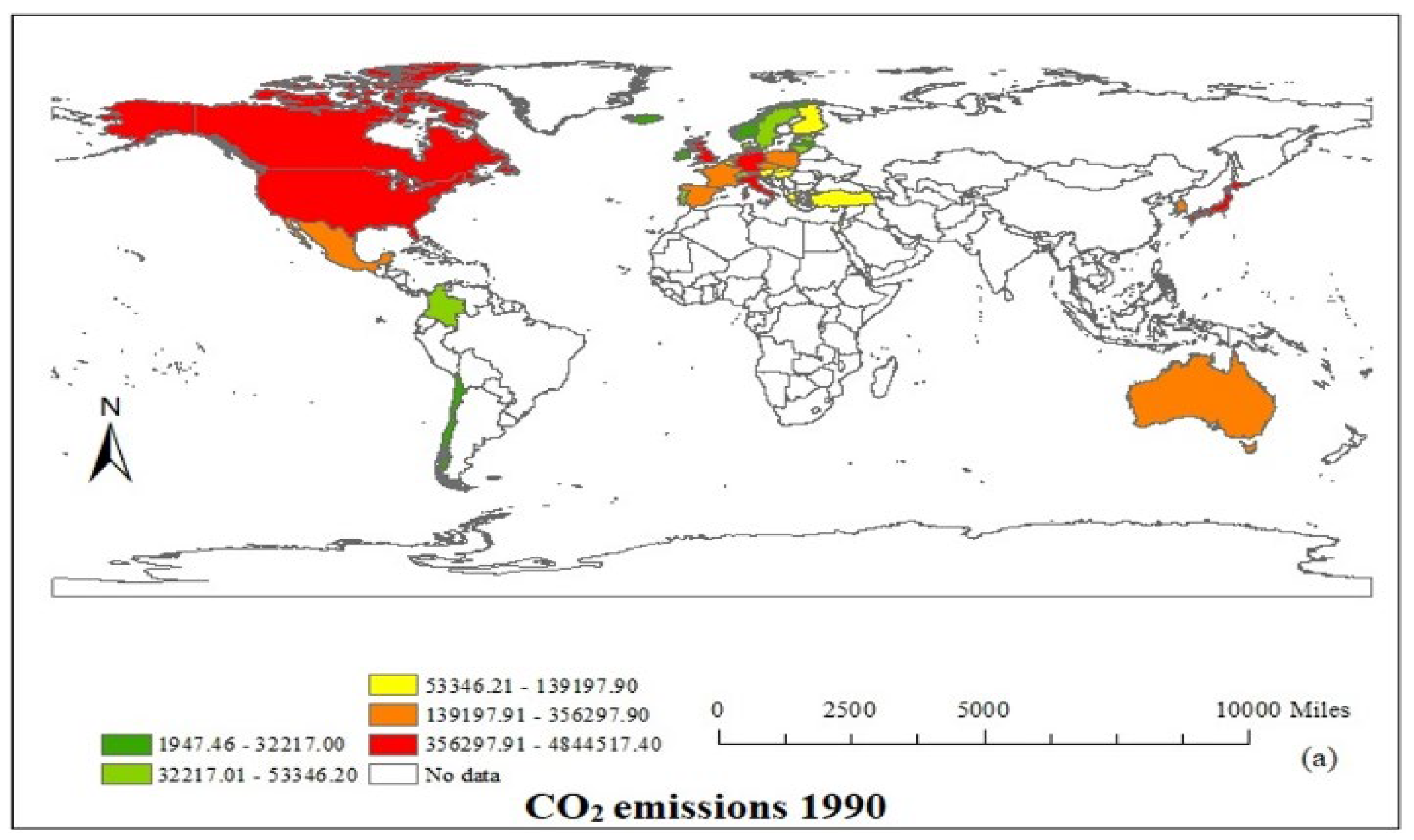
Figure 2.
CO2 emissions of OECD countries in 2019.
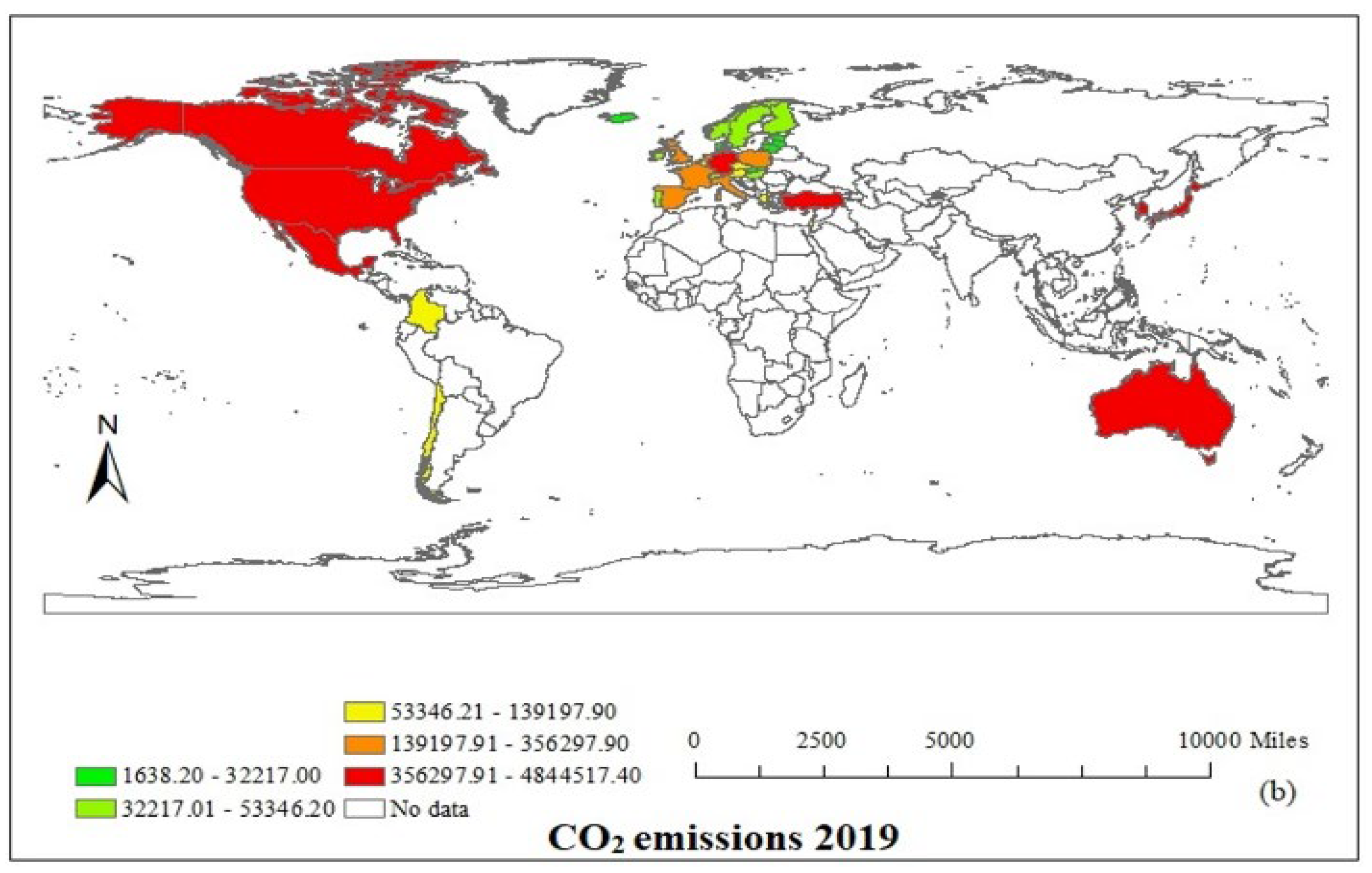
Figure 3.
Analytical framework of the study. Source: Authors’ illustration.
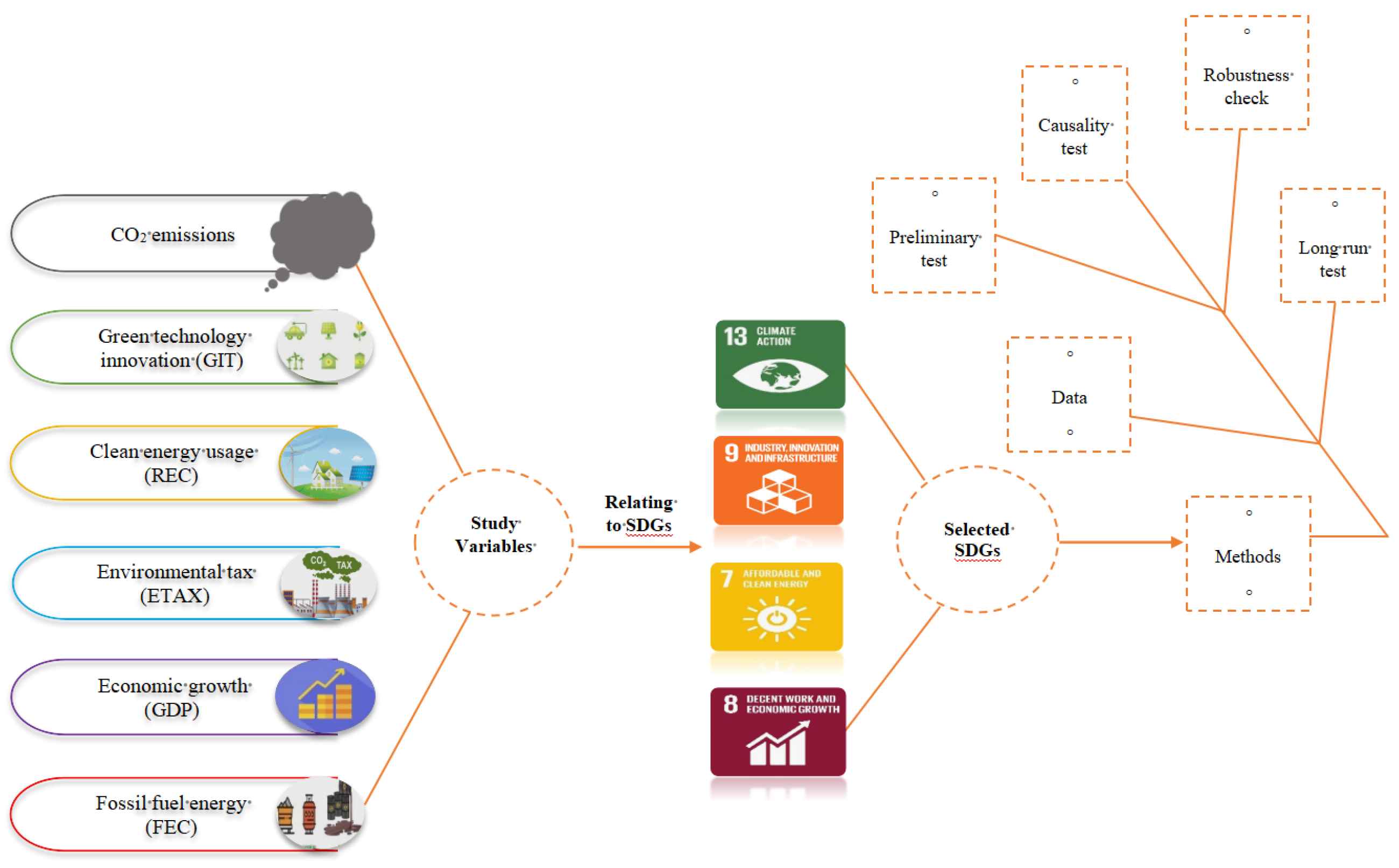
Figure 7.
Graphic display of long-run findings .
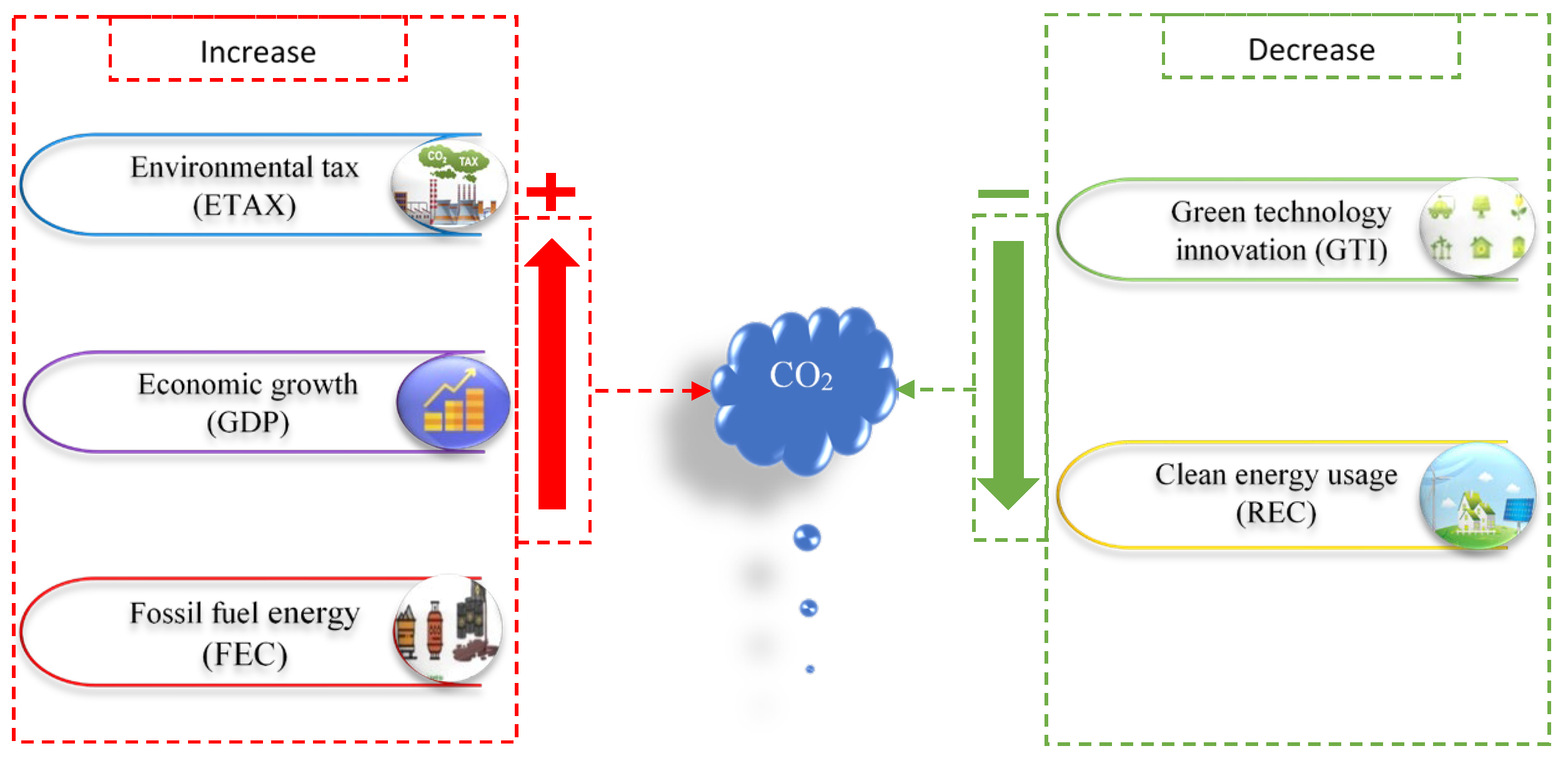
Figure 8.
Graphic display of causality findings.
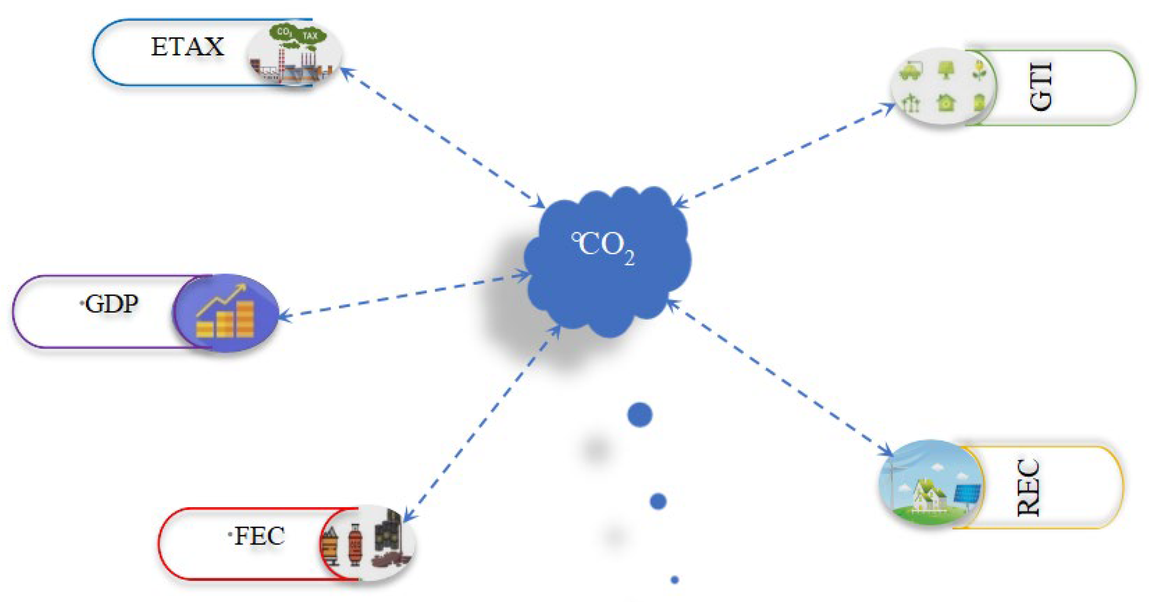

Table 1.
Description of study variables and databases.
| Variable | Definition | Unit | Database |
|---|---|---|---|
| CO2 | Carbon dioxide emission | Kiloton (kt) | WDI |
|
GTI |
Green technology innovation |
Number of patents for Environmental-related technologies |
OECD statistics |
| REC | Renewable energy consumption | % of total final energy | WDI |
| ETAX | Environmental taxes | Environmental taxes | OECD statistics |
| GDP | Gross domestic product per capita | Constant US 2010 | WDI |
| FEC | Fossil fuel energy consumption | % of total final energy | WDI |
Table 2.
Descriptive statistics of variables.
| Variables | CO2 | GTI | REC | ETAX | FEC | GDP |
|---|---|---|---|---|---|---|
| Mean | 11.531 | 4.168 | 2.375 | 0.766 | 4.248 | 10.111 |
| Median | 11.197 | 4.265 | 2.402 | 0.874 | 4.379 | 10.371 |
| Max. | 15.569 | 9.249 | 4.348 | 1.681 | 4.590 | 14.027 |
| Min. | 7.528 | -1.772 | -0.817 | -4.200 | 2.328 | 7.431 |
| Std. Dev. | 1.558 | 2.380 | 1.054 | 0.471 | 0.386 | 0.834 |
| Skewness | 0.020 | -0.021 | -0.480 | -2.639 | -2.510 | -0.521 |
| Kurtosis | 3.216 | 2.399 | 2.801 | 19.172 | 10.229 | 3.730 |
| Jarque-Bera | 2.111 | 15.868 | 42.030 | 12660.510 | 3388.843 | 70.795 |
| Probability | 0.348 | 0.000 | 0.000 | 0.000 | 0.000 | 0.000 |
| N | 1050 | 1050 | 1050 | 1050 | 1050 | 1050 |
| VIF | / | 2.29 | 1.68 | 1.08 | 1.55 | 2.17 |
Table 3.
Cross-sectional dependence test and homogeneity test.
| Variable | CSD-test | Correlation | ||
|---|---|---|---|---|
| CO2 | 13.91*** | 0.51 | ||
| GTI | 105.88*** | 0.79 | ||
| REC | 42.72*** | 0.70 | ||
| ETAX | 17.53*** | 0.62 | ||
| GDP | 95.41*** | 0.79 | ||
| FEC | 36.17*** |
0.62 |
||
| Slope heterogeneity test | ||||
|
|
Adjusted | |||
|
35.220 (0.000) *** |
40.225 (000) *** |
|||
Note: *** indicates statistical significance at 1%.
Table 4.
Results of the stationarity test.
| Variable | CIPS | Remarks | |||||
| Level | 1st difference | ||||||
| CO2 | -1.524 | -4.712*** | Stationary | ||||
| GTI | -2.606 | -5.042*** | Stationary | ||||
| REC | -2.209 | -5.023*** | Stationary | ||||
| ETAX | -1.291 | -4.944*** | Stationary | ||||
| GDP | -1.888 | -3.210*** | Stationary | ||||
| FEC | -2.406 | -5.272*** | Stationary | ||||
Note: *** indicates statistical significance at 1%.
Table 5.
Cointegration test results.
| Statistics | Value | Z-value | Robust p-value |
|---|---|---|---|
| Gt | -2.581*** | -3.508 | 0.000 |
| Ga | -11.625** | -2.358 | 0.009 |
| Pt | -14.616*** | -4.339 | 0.000 |
| Pa | -10.433*** | -4.833 | 0.000 |
Note: *** and **indicate statistical significance at 1% and 5%.
Table 6.
Long run results based on AMG and CCEMG.
| Variable | AMG | CCEMG |
|---|---|---|
| GTI | -0.019** (0.018) |
-0.023* (0.051) |
| REC | -0.210*** (0.000) |
-0.195*** (0.000) |
| ETAX | 0.033 (0.401) |
0.016 (0.586) |
| GDP | 0.404*** (0.000) |
0.337*** (0.000) |
| FEC | 0.835*** (0.001) |
0.632** (0.037) |
| Wald-Test | 62.34*** (0.000) |
49.55*** (0.000) |
Note: ***, **, and * indicate statistical significance at 1%, 5% and 10%. Values in parentheses are probability values.
Table 7.
Results of causality test.
| Null Hypothesis | Stats | tats |
|
Direction of causality | |||
|---|---|---|---|---|---|---|---|
| GTI CO2 | 3.279*** | 7.953 | 0.000 | ||||
| CO2 GTI | 3.574*** | 9.023 | 0.000 | ||||
| REC CO2 | 4.274*** | 11.556 | 0.000 | ||||
| CO2 REC | 4.592*** | 12.712 | 0.000 | ||||
| ETAX CO2 | 1.945*** | 3.122 | 0.002 | ||||
| CO2 ETAX | 3.602*** | 9.125 | 0.000 | ||||
| GDP CO2 | 3.610*** | 9.154 | 0.000 | ||||
| CO2 GDP | 3.053*** | 7.134 | 0.000 | ||||
| FEC CO2 | 2.769*** | 6.106 | 0.000 | ||||
| CO2 FEC | 2.625*** | 5.584 | 0.000 |
Note: *** indicates statistical significance at 1%.
Disclaimer/Publisher’s Note: The statements, opinions and data contained in all publications are solely those of the individual author(s) and contributor(s) and not of MDPI and/or the editor(s). MDPI and/or the editor(s) disclaim responsibility for any injury to people or property resulting from any ideas, methods, instructions or products referred to in the content. |
© 2025 by the authors. Licensee MDPI, Basel, Switzerland. This article is an open access article distributed under the terms and conditions of the Creative Commons Attribution (CC BY) license (http://creativecommons.org/licenses/by/4.0/).
Copyright: This open access article is published under a Creative Commons CC BY 4.0 license, which permit the free download, distribution, and reuse, provided that the author and preprint are cited in any reuse.


