
Submitted:
15 January 2026
Posted:
16 January 2026
You are already at the latest version
Abstract
Quantum computing has been rapidly evolving as a field, with innovations driven by industry, academia, and government institutions. The technology has the potential to accelerate computation for solving complex problems across multiple industrial sectors. Finance and economics, with many problems exhibiting computationally heavy requirements, is a high-profile sector where quantum computing could have a significant impact. Therefore, it is important to identify and understand to what extent the technology could find utility in the sector. This technical review is written for quantum applications researchers, quantitative analysts in finance and economics, and researchers in related mathematical sciences. It is divided into two parts: (i) a survey of quantum algorithms pertinent to problems in finance and economics, and (ii) mapping of several use cases in the sector to the potential quantum algorithms presented in part (i). We discuss some challenges on the pathway to achieving quantum advantage. Ultimately, this review aims to be a catalyst for interdisciplinary research that will accelerate the advent of the practical advantages of quantum technologies to solve complex problems in this sector.
Keywords:
quantum computing
; quantum algorithms
; fintech
; finance
; economics
1. Introduction
Quantum computing was first theorised in the 1970s [1], and the new research field gained more momentum after Feynman’s seminal talk [2]. At its core, quantum computing leverages the principles of quantum physics to process information. For problems that are intractable for classical computing, like simulation of complex quantum many-body systems, quantum computing is expected to solve them efficiently in a time frame that scales linearly with the system size [2,3]. In contrast, classical methods for such problems have computational times to solution that scale exponentially with system size. Furthermore, it was theorised that quantum computing could speed up computations for classically tractable problems like searching [4]. The landscape of proposed quantum algorithms that have speed-ups over their classical counterparts ranges from quadratic [4,5] to exponential [6,7]. Such theoretical discoveries, along with the rapid development of quantum hardware [8], have led many researchers to believe that quantum computing will have a significant impact across many disciplines and industry sectors.
In particular, in finance and economics, where complex calculations, large datasets, and optimisation problems are ubiquitous, quantum computing has the potential to improve computational efficiency for specific problem cases, provided certain conditions are met, such as efficient data loading and quantum error-correction [9]. For example, intricate models in finance for risk assessment, portfolio optimisation, fraud detection, and high-frequency trading, which generally require substantial use of high-performance computing, can potentially benefit from quantum computing. Similarly, economic modelling and simulation (particularly in macroeconomic forecasting, game theory, and market equilibrium analysis) could benefit from the integration of quantum processors in the computational pipeline. The expected gains with quantum computing methods are twofold: (i) large-scale, high-dimensional problems can be handled efficiently without resorting to many approximations and truncation as typically needed for classical computing approaches; and (ii) the computational time to solution can be significantly reduced, and accuracy improved for some categories of problems [10]. However, there are a few current bottlenecks in realising these potential gains, which include the challenge of efficiently loading and reading out data from a quantum computer [11,12].
This review explores some of the promising use cases in finance and economics where quantum computing could have a significant impact. We discuss the theoretical foundations of pertinent quantum algorithms, recent proof-of-concept implementations, and potential future implications. By examining these specific use cases, such as option pricing and risk management, this review highlights both the opportunities and limitations of quantum computing in the context of the aforementioned sectors. We aim to provide an objective analysis, providing a technical review of key quantum algorithms, corresponding use cases, and the overall state-of-the-art of quantum computing for finance and economics.
1.1. Motivation and Contributions
This review seeks to provide a bridge between use cases, as encountered by practitioners in finance and economics, and their potential solutions using quantum computing. This survey contributes towards stimulating interdisciplinary research to accelerate the development and demonstration of quantum computing advantage for applications in these sectors.
What is meant by advantage in quantum computing is often debated, since there is currently no unique definition for it. There are generally three terms commonly used in association with quantum advantage:
- Computational Advantage - also referred to as Quantum Supremacy [13], is a point where quantum computers can efficiently perform a task that is intractable for a classical computer. The task does not have to be directly useful for real-world applications, such as efficient random sampling from a particular probability distribution [14,15,16,17].
- Quantum Utility - a point when quantum computers can solve a problem more efficiently than classical brute force methods. This definition was first introduced by IBM Quantum in association with their work in simulating spin systems [18].
- Practical Quantum Advantage - a point where quantum computers can solve a problem more efficiently than the most advanced classical methods. In this case, the problem/task in question has real-world practical application(s) and impact in areas such as logistics, healthcare, finance, and economics.
Therefore, most researchers consider Practical Quantum Advantage (PQA) a monumental milestone that will unlock the benefits of quantum computing to the growth of the economy and society at large. Oxford Economics has quantified these benefits as an economy-wide productivity boost, which is projected to be up to 8.3% by 2055 in the UK, with initial gains from as early as 2034 [19]. Under reasonable assumptions, this is equivalent to each worker in the UK producing an extra one and a half weeks’ worth of output annually, without putting in any additional hours [19]. Furthermore, the report estimates that by 2055, the quantum computing industry will contribute between £5.9 billion and £12.9 billion in total gross value added to the UK’s GDP [19]. Globally, McKinsey [20] has projected that applications of quantum technologies in finance will contribute a total value of $622 billion by the year 2035. Hence, some analysts have predicted that the financial services sector will be one of the first industries to reap the benefits of quantum technologies [21].
Since the general expectation is that quantum computing will generate a lot of value both in the UK and globally, the key question is what is a viable path towards PQA? What are the hardware engineering and software algorithmic hurdles to overcome to achieve PQA? And what could accelerate the collaborative effort towards that common goal? This review seeks to contribute towards answering these questions by providing:
- 1.
- A survey of state-of-the-art quantum algorithms with potential applications in finance and economics.
- 2.
- A mathematical outline of use cases in the aforementioned sectors and viable quantum approaches towards an efficient solution. Note that this review is among the first to extend the scope of such a survey to cover use cases in economics.
- 3.
- A discussion of the technical challenges towards realising PQA of quantum computing applications in these sectors.
The following subsections outline how our contribution adds to previously published related survey reports and the benefits of the structure of this review.
1.2. Related Survey Reports
The interest in quantum computing use cases in finance is evident in the rapidly growing number of publications and investments in the field. The total number of papers, articles, and theses written on quantum computing for finance has grown from under 2,000 in 2014 to over 10,000 in recent years [22]. Commensurate with the growth of the field, regular survey reports of quantum computing in finance progressed from general overviews in the years 2019 to 2020, to specialised applications in Quantum Machine Learning and financial modelling in the years 2021 to 2024. This is a reflection of the field shifting toward practical implementations, with increasing focus on derivatives pricing, risk assessment, and quantum-enhanced financial strategies. Table 1 presents a sample list of related survey reports of quantum computing applications in finance from 2019 to 2025.
Each of the survey reports above is written for a specific audience, as reflected in the depth of technical details covered and the emphasis on either quantum algorithms or financial use cases. In this review, our approach is to present the technical depth of the key quantum algorithms and the mathematical formulation of the use cases in finance and economics. We hope this approach will spur interdisciplinary collaboration that will accelerate the advent of PQA for industrial applications.
1.3. Structure of the Review
The structure of the review resembles the mapping between use cases and problem domains shown in Figure 1.
Thus, we have divided this report into three parts:
- Part I:
-
Quantum algorithms - a review of the key quantum algorithms with potential PQA in finance and economics. These are grouped into four problem domains:
- (a)
- Simulation algorithms are presented in section (2.2), including Quantum Monte Carlo Integration and quantum solvers for Stochastic Differential Equation.
- (b)
- Optimisation algorithms are presented in section (2.3), particularly for combinatorial and convex optimisation problems with state-of-the-art examples.
- (c)
- Quantum Machine Learning algorithms are presented in section (2.4), which are quantum extensions of classical Machine Learning techniques for supervised, unsupervised, and reinforcement learning.
- (d)
- Quantum cryptography methods are presented in section (2.5), including a discussion of future expected threats to cybersecurity posed by quantum computers once the technology reaches full maturity, and some quantum-safe protocols for data encryption and communication.
The pertinent primitive algorithms that feature as subroutines to quantum algorithms in the above problem domains are outlined in section (2.1). - Part II:
-
Use cases in finance and economics - a review of the mathematical formulations of potential use cases of quantum computing in finance and economics. These are grouped into three parts:
- (a)
- Banking and Investment - presented in section (3.1), we identify some of the computational bottlenecks for classical methods in banking and investment problems, and use cases where quantum computing can potentially have an advantage. These include pricing assets and derivatives, portfolio optimisation, hedging, and arbitrage.
- (b)
- Risk Management and Cybersecurity - presented in section (3.2), we identify some of the simulation and security challenges in risk management and cybersecurity, respectively. Similar to banking and investment, we present the technical formulations of use cases of quantum computing in this category. This includes quantum approaches for risk analysis (Value-at-Risk, credit scoring, etc.) and fraud detection.
- (c)
- Economics - presented in section (3.3), the mathematical formulation of potential use cases of quantum technologies for problems arising in economics is outlined. These include quantum money and macroeconomic forecasting.
- Part III:
- Summary and outlook - of this report is presented in section (4), in which we reiterate the benefits to financial organisations in working towards quantum readiness, and provide an outlook of one possible route towards PQA.
Note: This review is not a comprehensive review of all quantum algorithms nor use cases in finance and economics. We have selected a subset of use cases that represent areas of potential high impact with some current published research activity in the form of proof-of-concept proposals and/or demonstrations. Similarly, we have chosen to give technical details for simpler formulations of quantum algorithms for a problem domain and mention more complex approaches in passing. Furthermore, this review is also not intended as a primer on quantum computing or quantum information theory. In the quantum-specific sections, we assume a level of familiarity with quantum mechanics and related terminology, which other sources will be able to provide in more detail. In the next section, we will summarise some of the notation used in this review for the reader’s convenience. Finally, we hope that financial organisations interested in incorporating quantum technologies can work with quantum applications engineers to develop relevant solutions using this survey and others as a starting point.
1.4. Notation
In this section, we summarise some of the key notation used in this review for clarity. This is not an exhaustive list, and some of the notation can be overloaded when the meaning is clear in the context. For example, in some parts of the text, the Hamiltonian may be denoted as H, and it should not be confused with the Hadamard gate. Similarly, the Big-O notation may be denoted as or , which both mean the same thing. Table 2 gives a sample of common notation in quantum computing and analysis of quantum algorithms that are used in this review. Since this review is not an introductory text in the field, a reader who is unfamiliar with these notations can refer to Ref. [44] for more information.
2. Quantum Algorithms
2.1. Primitive Quantum Algorithms
This section offers an introduction to a set of quantum algorithms, here referred to as primitive algorithms, that are used as the basis or fundamental building blocks from which more complex quantum algorithms, models, or frameworks are constructed [47]. As primitive algorithms do not directly solve an end-to-end problem, groups of these fundamental algorithms (also called subroutines) are needed to create a wide range of high-end quantum applications [48].
2.1.1. Quantum Phase Estimation
One of the earliest quantum algorithms to be discovered is the Quantum Phase Estimation (QPE), which was first formalised in 1995 by Kitaev1 [50]. This subroutine has been widely used by many other algorithms, including Shor’s quantum algorithm for factoring large numbers [49,51], Hamiltonian diagonalisation [52], and solving systems of linear equations [6].
QPE serves as a key building block for quantum algorithms, of which some have a potential quantum speed-up that is exponential due to it. The objective of the algorithm is the following [44]: given a unitary operator U, estimate the phase in the representation
Here is an eigenvector and is the corresponding eigenvalue. To implement the QPE, the quantum system needs to be separated into registers: the state register that contains and the phase register that contains the encoded estimate of the phase . The QPE subroutine is constructed as follows:
- 1.
- Setup: initialise the state register with the state . The additional set of n qubits that form the phase register is set in state . After initialisation, the global state of the system will be:
- 2.
- Superposition: an n-bit Hadamard gate is applied on the phase register, leaving the global state as:
- 3.
-
Controlled Unitary Operations: consider a controlled unitary that applies the unitary operator U on the target register (i.e., the phase register) only if its corresponding control qubit is [44]. Since U is a unitary operator with eigenvector such that , it follows that:Applying all the n-controlled operations with , and using the relation , leads to the global state:where k denotes the integer representation of n-bit binary numbers.
- 4.
- Inverse Fourier Transform: The Quantum Fourier Transform (QFT) maps an n-qubit input state into:The expression of the global state is the result of applying QFT on the global expression of Step 2. Therefore, to recover the state , an inverse Fourier transform is applied on the phase register [53]. Doing so, it is found that
- 5.
- Measurement: the above expression peaks near . For the case when is an integer, measuring in the computational basis gives the phase in the phase register with high probability, as the global state now is:For the case when is not an integer, it can be shown that the above expression still peaks near with probability at least [44].
Algorithm (1) summarises the key steps of the QPE subroutine which scales as , for desired additive error [50]. The standard QPE circuit requires controlled- operations, which can be a resource challenge for current Noisy Intermediate-Scale Quantum (NISQ) hardware. Hence, QPE is considered a Universal Fault-Tolerant (UFT) quantum algorithm which requires Quantum Error Correction (QEC) to obtain highly accurate phase estimates. In the NISQ era, practitioners often employ approximate versions of QPE with reduced circuit depth and error mitigation methods to suppress effects of noise. These variants of QPE include the Iterative Quantum Phase Estimation (IQPE), which uses a single control qubit repeatedly and employs classical post-processing to update estimates of [54]. IQPE typically has the same asymptotic error scaling but requires fewer qubits [54], making it more suitable for near-term quantum devices. There have also been proposals for alternatives to QPE such as the quantum eigenvalue estimation via time series analysis [55] and the phase estimation of local Hamiltonians [56]. These methods used expectation values of the evolution operator for various times to estimate the eigenvalues of a Hamiltonian, which makes them more feasible to implement on NISQ hardware.
| Algorithm 1 Quantum Phase Estimation |
|
Initialising. Initialise the quantum system. There exist two qubit registers, the phase register initialised in state , and the state register initialised in .
Superposing. Apply Hadamard gates on the phase register.
Applying the unitary. Apply the controlled unitary operation as shown in the third step of the mathematical analysis.
Inverse QFT. Apply the inverse quantum Fourier transform to decode the state of the phase register.
Measure. Measure the phase register to get an approximation of the desired phase, .
|
2.1.2. Quantum Amplitude Algorithms
Another set of widely used quantum subroutines introduced by Brassard et al. [57] are the Quantum Amplitude Amplification (QAA) and Quantum Amplitude Estimation (QAE). These algorithms are an extension of the principles of Grover’s search algorithm [4] to a broader range of applications.
Quantum Amplitude Amplification
The first amplitude subroutine, QAA, also used within Grover’s search algorithm [4], enhances the probability amplitude of desired outcomes within a quantum algorithm. The QAA generalizes Grover’s unordered search to any algorithm with a known success probability [58], enabling a potential quadratic speed-up over classical repetition strategies [57].
Consider a quantum algorithm that produces a state
where is the `good’ subspace (desired states), a the probability of measuring a `good’ state, and the `bad’ subspace. The amplification process is done using the Grover-like operator , which acts as a rotation and is defined to be [57]
where
The operator reflects about the initial state, which flips the sign of the amplitudes of the good states if and only if . The operator reflects about the good state which flips the sign of if and only if . This implies that [57]
The probability amplitude of the good state is where , with , and the optimal m number of iterations is . Applying Q iteratively to , the state evolves such that after m applications, the state is
Thus, Q rotates the state in the plane per each iteration. If a is known, QAA achieves a quadratic speed-up with applications of and . For unknown a, quantum search algorithms like one outlined in Section (2.1.3) use exponentially increasing numbers of iterations to find a good solution. This approach is also expected to use same applications and if [57]. Algorithm (2) summarises the QAA subroutine using the operator Q and a general algorithm.
| Algorithm 2 Quantum Amplitude Amplification |
|
Initialise: Apply a quantum algorithm to to prepare the state:
Amplify: Define the amplification operator and apply it to m number of iterations to rotate the state:
Measure: Measure the final state to obtain a good state.
Repeat: If a is unknown, use exponentially increasing m until a good state is found.
|
An extension of QAA, called the variable time amplitude amplification, which can be decomposed into multiple steps with different stopping times [59], has been applied as a subroutine that improves the complexity of Harrow et al. [6] Quantum Linear Systems Solver. Improvements to the QAA subroutine have been proposed, such as the oblivious amplitude amplification [60] which handles the issue that occurs when it is not possible to perform the required reflection about the state . Another version of QAA is the fixed-point amplitude amplification [61] that ensures amplitude amplification happens regardless of an unknown amplitude. These improved versions of QAA are subroutines for Quantum Singular Value Transformation (QSVT) methods [62] and have been recently compared in the Hamiltonian simulation problem [63].
Quantum Amplitude Estimation
The second amplitude subroutine, QAE algorithm first proposed by [57], is closely related to QAA and seeks to estimate the probability amplitude of a specific outcome with high precision. It is a key subroutine for a broad class of Monte Carlo-like estimation tasks [64] and offers a potential quadratic quantum speed-up [5].
The QAE can be described similarly as QAA. Consider an algorithm that outputs a state given by Equation (2), the QAE seeks to produce an estimate for the amplitude a of the good state , where . Using the operator Q given by Equation (3), QAE estimates the value of a by using QPE to find the eigenvalues of Q [57]. Hence, both QAA and QAE use the operator Q, but the former boosts a for measurement of , while the latter quantifies a itself.
The key idea is to assign the value of a to an angle so that the estimate of to a given precision using QPE gives us the estimate of a. This is done by setting and then applying QPE to the controlled-Q operations, since Q acts as a rotation in with eigenvalues . The estimate with M evaluations has errors bounds given by [57]
with probability at least for , and higher for . Algorithm (3) summarises the QAE that utilises QPE.
| Algorithm 3 Quantum Amplitude Estimation |
|
Initialise: Apply a quantum algorithm to to prepare the state: (same as QAA).
Define: Define the amplification operator Q given by Equation (3). The eigenvalues of Q are where for .
Estimate: First apply a total of M controlled-Q operations on state such that
Let , then apply QPE to estimate the eigenphase which we use to recover the amplitude
|
This version of the QAE algorithm is relatively resource-expensive due to the use of QPE, which uses many ancilla qubits for a good estimate, multiple controlled-Q operations, and the inverse QFT. Hence, this results in deep circuits which are not feasible to run on near-term devices. Some variants of QAE that do not make use of QPE include the Maximum Likelihood Amplitude Estimation [65], Faster Amplitude Estimation [66], Iterative QAE [67], Variational QAE [68], and low depth algorithms for QAE [64] which are more feasible on near-term devices. An important application of QAE to finance is to perform Monte Carlo integration, which will be discussed in more detail in Section (2.2.1). Other applications of QAE include general numerical integration [69], estimating the probability of success of a quantum algorithm [70], and approximate counting [71].
2.1.3. Quantum Unstructured Search (Grover’s Algorithm)
First proposed in 1996 by Lov Grover [4], the Quantum Unstructured Search (QUS)2 algorithm utilises the QAA subroutine to potentially obtain a quadratic quantum speed-up over classical methods for searching an item in an unstructured dataset.
In this section, we describe the key idea behind the QUS algorithm. For a database of entries, let be the set of items in an array, and w the marked item (i.e., the item the routine searches for). Let f be a function such that if and only if and otherwise. The quantum states can be encoded as binary strings . One can then define the oracle acting on a quantum state, , as
Thus, the oracle does nothing to the unmarked quantum states and negates the phase of the marked state . Geometrically, the unitary matrix of this oracle corresponds to a reflection about the origin for the marked item in an N-dimensional vector space.
The QAA subroutine provides the quadratic speed-up of QUS by amplifying the amplitude (and thus, the probability) of the target quantum state, making it more likely to appear after measurement. This procedure is summarised in Algorithm (4) and has been shown to have a query complexity of , which is a quadratic speed-up over classical brute force methods of [4].
| Algorithm 4 Quantum Unstructured Search (Grover’s Algorithm) |
|
Initialisation: Start with , apply Hadamard gates to create a uniform superposition:
Each state has amplitude .
Oracle Application: Apply the oracle , which flips the phase of solution states, such that for one solution , the state becomes:
This marks solutions by changing their sign.
Diffusion Operator: Apply the diffusion operator , where I is the identity. This reflects the state over , amplifying solution amplitudes:
The action of the Grover operator is to amplify the amplitude of the solution state.
Iteration: Repeat the Grover operator k times and then measure to find highest probability state . The optimal k receptions to maximise the probability of finding the target state(s) is approximately:
|
Grover’s algorithm has been applied as a subroutine for various applications, including speeding up nested search of structured problems [72], stochastic pure adaptive search for unconstrained global optimization [73], high-energy physics data at the Large Hadron Collider [74], image pattern matching [75], and homomorphic encryption schemes [76]. The QUS algorithm as described here is considered a fault-tolerant quantum algorithm due to the deep circuits (required to reach optimal k iterations) which are infeasible to run successfully on current NISQ hardware. Hence, similarly to the other primitives reviewed here, improvements have been suggested to the QUS to make it amenable to run on near-term quantum hardware. These include the divide-and-conquer strategy and partial diffusion operators to reduce circuit depth and error accumulation [77,78], as well as variational approaches [79,80].
2.1.4. Quantum Walks
Random walks have long served as a foundational model in the study of stochastic processes, with applications spanning physics, computer science, biology, and finance. In its classical form, a random walk describes the trajectory of a particle that takes successive steps in random directions, typically governed by a Markov process [81]. Random walks have also been generalised to graphs [82], in which case they can be viewed as finite-state Markov chains over the set of vertices [83]. A simple example is the one-dimensional symmetric random walk, where a particle at position moves to or with equal probability at each time step. In finance, the Geometric Brownian Motion (GBM) is a widely used random walk for modelling market stochastic quantities like asset prices [84,85].
The quantum analogue of random walks, known as quantum walks, emerged in the early 1990s as a framework for modelling quantum dynamics and as a potential basis for quantum algorithms [86]. Unlike classical random walks, quantum walks evolve according to unitary transformations, preserving coherence and allowing for interference between paths. This leads to fundamentally different behaviour, including faster spreading and potential algorithmic advantages [87].
Two main formulations of quantum walks exist: discrete-time and continuous-time. The Discrete-time Quantum Walk (DTQW) was first formalised by Aharonov et al. [86], incorporating a coin space to account for internal degrees of freedom. In contrast, the Continuous-time Quantum Walk (CTQW), introduced by Farhi and Gutmann [88], operates directly on the graph structure without an explicit coin. In this section, we will review the key ideas behind quantum walks, beginning with their mathematical foundations and then exploring their distinctive dynamical properties, algorithmic formulations, bottlenecks, and applications.
Discrete-Time Quantum Walks
Consider a walker on a 1D line, flipping a quantum coin to decide whether to turn left or right at each step. This represents one of the simplest quantum walks, also referred to as a qubit walk on a finite cycle (with N states) in discrete time [89]. This quantum walk can be described by repeated application of a unitary evolution operator U which acts on the Hilbert space composed of the coin qubit (C) with basis and state space (S) with basis for , respectively. The unitary U is defined as [89]:
where S is the conditional shift operator given by [90]
The operator moves the walker one step to the right, increasing its position, and to the left, decreasing its position. The quantum coin operator C is can be chosen to the Hadamard gate H, such that
We note that although this coin is unbiased3, the quantum walk from this coin operator () will be asymmetric with bias towards rightward paths. This is because the leftwards path () undergoes more destructive quantum interference, whereas the rightwards path undergoes more constructive quantum interference [91]. This phenomenon has no classical analogue and makes quantum walks more expressive than classical random walks [86,87]. The coin represented by the Hadamard operator alongside a step operator causes the probability amplitude to become distributed over an increasing space in discrete jumps [92]. This asymmetry can be overcome by choosing a balanced coin operator [87], for example
which treats both and the same, independent of the initial coin state.
Intuitively, in each step, the qubit first ’splits’ into two paths (C puts it in a superposition) and then one ’half’ steps leftwards, while the other steps rightwards. This process, when repeated with T-steps, produces a probability distribution that is ballistic with standard deviation , whereas the classical random walk has a diffusive distribution with standard deviation [87]. This implies the quantum walk propagates quadratically faster than classical walks [87], which means they can explore more of a graph in fewer steps than classical random walks [93].
Generally, quantum walks in discrete time can be viewed as a Markov chain over the edges of a graph and consist of a series of interleaved reflection operators [94,95]. This formulation of quantum walks generalises the QAA and Grover’s algorithm discussed in Sections (Section 2.1.2.1) and (Section 2.1.3), respectively [96,97]. The bipartite character of the graph introduces the modularity property of quantum walks (similarly to classical random walks), which is that after an even (odd) number of steps, the probability to find the walker on odd (even) positions is always zero [98]. This property allows for simplified analysis of the performance of quantum walks, in particular, to two important metrics: the mixing time and hitting time of random walks on graphs. The mixing time of a graph is the time it takes for a random walk on the graph to become close to the stationary distribution; that is, the point where the walk "forgets" where it started and behaves as if it started from a random node [99]. The hitting time from node u to node v is the expected number of steps a random walk starting at u takes to reach v for the first time [81]. Quantum walks are shown to potentially have a polynomial quantum speed-up in mixing times [89,93,100] and hitting times for Markov-chain-based search algorithms [94,95,101,102,103,104,105] than their classical random walks counterpart. There have been several proof-of-concept implementations of DTQW on NISQ hardware, which include a Hadamard-based on the 4-cycle and 8-cycle [106] and extensions to multi-qubit systems [107,108].
Continuous-Time Quantum Walks
Consider an undirected graph , where V is the set of its vertices and E the set of its edges. In classical mechanics, a diffusion equation can be used, which allows probability to leak to or from neighbouring vertices. The number of neighbouring nodes equals the degree of the node j, or . This diffusion operation can be expressed as
where t is an arbitrary continuous time parameter, is a function that describes the probabilistic exchange between node j and its neighbouring nodes. The operator L is symmetric and Hermitian, called the Laplacian of G, given by
Thus, since L is a Hermitian matrix, it can play the role of a Hamiltonian in Schrödinger’s equation as
where, for simplicity it can be assumed that and is the state of the system at arbitrary time t. First introduced by Farhi and Gutmann in [88], Equation (14) represents the Continuous-time Quantum Walk (CTQW). As evident from the above formulation, the CTQW does not need a quantum coin that drives the evolution, unlike the DTQW. This makes CTQW a construct that shares dynamics with the DTQW, but exhibits different behaviour. In contrast to the quantum coin tossing example described in Section (2.1.4.1), the walker now moves smoothly (or continuously), guided by an evolution rule (which is driven by the Hamiltonian, typically the graph Laplacian L). This evolution follows the Schrödinger Equation (14) and the walk is continuous without distinct steps. Therefore, we can summarise the fundamental differences between the two quantum walks as:
- State space: CTQWs require only the vertex space, while DTQWs models need an auxiliary coin space for evolving. As described in Section (2.1.4.1), the coin operator drives the symmetry or asymmetry of the quantum walk.
- Dynamics: CTQWs have continuous Schrödinger evolution (via Hamiltonians), whereas discrete-time walks rely on alternating coin and shift operators per time step.
In addition, the various mixing operators used in Quantum Approximate Optimisation Algorithm, described in Section (2.3.1.4), can be viewed as CTQW connecting the feasible solutions [109]. Similarly to DTQWs, the CTQWs can showcase a quadratic advantage in terms of accelerating diffusion (i.e., spreading) compared to classical continuous-time random walks [110]. For some oracular graph problems, the CTQW can theoretically achieve exponential advantage over classical methods [111].
It was shown by Childs that CTQW can be regarded as a universal computational primitive, with any quantum computation encoded in some graph [112]. Later, Lovett et al. [113] showed that the DTQW can also achieve universal quantum computation. Hence, there have been multiple proposed unifications of quantum walks in continuous and discrete time [114,115], something that is true for the classical versions [116]. For a comprehensive review of quantum walks, see the survey in [115]; and for an overview and a discussion of connections between the various quantum-walk-based search algorithms, see the work by [103].
Quantum walks have since found applications in a variety of areas, including quantum search algorithms [97], modelling transport in biological systems [117], and many others [110]. Their utility stems from the combination of quantum superposition and interference, which enable new algorithmic paradigms not feasible in classical settings. Current research into quantum walks faces many challenges. As in any other quantum algorithm, a significant issue is implementation on NISQ devices where noise can disrupt the coherent evolution required for quantum walks. Efforts to mitigate these decoherence effects have been explored in various studies, such as [118], which simulate quantum walks of interacting particles and demonstrate topological protection against noise. However, achieving scalable quantum walks on large graphs, or lattices, remains a challenging task [110], as current hardware limitations restrict the size and duration of coherent quantum evolutions.
2.1.5. Quantum Linear System Solver
Linear systems of equations are ubiquitous in science, engineering, and mathematical fields. There are several numerical methods developed over the years for solving them efficiently on classical computers [119,120,121]. The general Linear Systems Problem (LSP) can be formally defines as:
Definition 1
(LSP). Given a matrix and a vector , find a vector s.t. , or indicate that the system has no solution.
In other words, Definition (1) describes a matrix-inversion problem since the solution is given by . The Quantum Linear Systems Problem (QLSP) is quantum version of the LSP, and is defined as:
Definition 2
(QLSP). Given a matrix and and a vector , prepare the state on a quantum computer with qubits such that
where ϵ is the desired precision. The target quantum state with
where are the component of vector b.
One of the key differences between the LSP and QLSP is that the former outputs the full solution vector x whilst the latter outputs a normalized vector proportional to the solution . Table 3 shows the time complexity of the best known classical algorithm for solving the LSP, with A matrix sparse [122] and dense [123], compared with a few quantum algorithms for solving the QLSP.
HHL Algorithm In this section, we will consider the Harrow-Hassidim-Lloyd (HHL) algorithm [6] which is the first quantum algorithm for solving the QLSP. As mentioned earlier, it does not provide the whole solution vector, but a quantum state proportional to the solution, which we can sample from with relatively low additional error. Given that the coefficient matrix A is sparse and well-conditioned, the quantum algorithm can potentially achieve an exponential quantum speed-up in the dimension of the matrix N compared to the best known classical algorithm [6]. However, there are caveats for this speed-up to be possible, which include [6,11] the following conditions:
- 1.
- Matrix A must be sparse or can be efficiently decomposed into a sparse form.
- 2.
- The condition number of A must be small and scale as .
- 3.
- The elements of A can be efficiently utilized via black-box oracle calls as needed.
- 4.
- The final output is the case where one does not need to know the solution itself, but rather an approximation of the expectation value of some operator associated with , e.g., for some matrix M.
It may seem that these constraints, alongside other challenges in quantum computation restricts the possibility of having a PQA as noted by Aaronson [11]. Ongoing research [133] and improved versions of HHL, such as shown in Table 3, are promising to deliver PQA.
The main steps of the algorithm are (i) phase estimation, followed by (ii) a controlled rotation, (iii) uncomputation, and, finally, (iv) measurement and post-selection [133]. A summary of the HHL algorithm is provided below, and for more information, the reader is referred to [6,133]. Consider the matrix A that is s-sparse and Hermitian, then its spectral decomposition is given
where is the eigenvector of A with respective eigenvalue . In this decomposition, the matrix inversion of A is then given by
We can express in the eigenbasis of A as
where we already have an implicit normalisation constant since we are talking about a quantum state. The goal of the HHL is to exit the algorithm with the readout register in the state approximately , which can also be expressed in the eigenbasis of A as
Therefore, the HHL algorithm encodes A into a unitary U given by
Thus, by applying QPE, one can implement the mapping
where is the binary representation of up to a tolerated precision. Following this, the implementation of a controlled rotation takes place conditioned on . This requires an ancilla register, S, which is added to the system initialised in state . The controlled rotation is of the form of a -rotation (i.e., a rotation around the y-axis or quantisation axis) and produces a normalised state of the form.
where c is a normalisation constant. This can be achieved through the application of the quantum operator
where . Thus, enacting the procedure described above in the latter superposition, it is derived that
Finally, the first register is uncomputed, giving
Following the uncomputation, we see that the state of the system (including all the quantum registers) is , or in other words, it exists in a state that is close to the solution . The state can be reconstructed within the clock register, C, by measuring the ancilla register, S, and post-selecting on the outcome 1 modulo the constant factor of normalisation, c. The success probability of the final step can be boosted using QAA. This procedure is summarised in Algorithm (5).
| Algorithm 5 Harrow-Hassidim-Lloyd algorithm for QLSP |
|
Input. Encode the state vector and the matrix A with oracular access to its elements. Define , and as the desired precision.
Initialise. Prepare the input state , where .
Hamiltonian. Apply the conditional Hamiltonian evolution following the input state.
Apply QFT to the register C, denoting the new basis states , for . Define .
Controlled rotation. Append the ancilla register, namely S, and apply a controlled rotation on S with C as the control register, mapping states . The state is defined in such a way that it produces an output which denotes whether an inversion has occurred and if that inversion is well-conditioned or not [133].
Uncomputation. Uncompute the register C.
Measurement. Measure the register S.
Repeat. Perform rounds of QAA on the HHL algorithm.
Output. Result is the state s.t.
|
The HHL algorithm was the first QLSS and, as shown in Table 3, there have been many improvements on it up to the recent ones with optimal scaling in and [131,132]. It is worth noting these state-of-the-art quantum algorithms for the QLSS with optimal scaling for the case when A is sparse, and there have been a few proposals for the case when A is dense. For the latter case, Wossing et al. [126] utilised the Quantum Singular Value Estimation (QSVE) algorithm of [134] to achieve a polynomial speed-up over the best known classical algorithm based on powers of tensors with subcubic complexity [123]. However, as noted in [126], the classical algorithm with subcubic complexity [123] is difficult to achieve in practise hence, for the dense matrix case, the Cholesky decomposition with complexity [135] is often used. This implies that for problems with non-sparse A matrix, such as kernel methods and neural networks in machine learning [136], the potential exponential quantum advantage of HHL-type quantum algorithms is lost.
Following this, Kerenedis and Prakash generalised the QSVE-based linear systems solver to handle both sparse and dense matrices and introduced a technique for spectral norm estimation [137]. Another general framework for solving the QLSP is the Quantum Singular Value Transformation (QSVT) [138], which uses an iterative least square algorithm and has been proposed [139,140]. Although this algorithm does not have optimal scaling with and , it is general in the sense that it does not assume that A is invertible nor that it is a square matrix, but uses the Moore-Penrose pseudoinverse [141] such that the output is achieved efficiently [48,139,140]. Furthermore, the QSVT also provides a general framework that unifies [62] a variety of quantum algorithms, such as linear algebraic subroutines like singular-value-threshold projectors [134,138] and matrix-vector multiplication [139]. An outline of QSVT is presented in Algorithm (6).
| Algorithm 6 Quantum Singular Value Transformation |
|
Input: A block-encoding of matrix A, i.e. ; a definite-parity polynomial of degree d; and a phase sequence from polynomial synthesis.
Construct QSVT sequence: Let , and define
This yields a block-encoding of with the corresponding odd/even forms.
Linear combination: Using that implements , define
Output: that is a block-encoding of .
|
While solving the QLSP does not provide classical access to the solution vector, this can still be done by utilising methods for vector-state tomography with a cost of samples [142]. Applying tomography would no longer allow for an exponential speed-up in the system size N [11]. However, polynomial speed-ups with tomography for some linear algebra-based algorithms are still possible for certain types of problems [48]. In addition, without classical access to the solution, certain statistics, such as the expectation of an observable with respect to the solution state, can still be obtained without losing the exponential speed-up in N [6,143]. Another current bottleneck for QLSS is loading the data of A and b into quantum gates and states, respectively [11]. In theory, this can be dealt with by using one of the two main quantum models for data access [48,139]: (i) the sparse-data access model and (ii) the quantum-accessible data structure. The sparse-data access model provides efficient quantum access to the nonzero elements of a sparse matrix. The quantum-accessible data structure, suitable for fixed-sized, non-sparse inputs, is a classical data structure stored in a quantum memory (e.g., Quantum Random Access Memory (QRAM)) and provides efficient quantum queries to its elements [139]. Considering the cost of QRAM with QEC overheads [144], the potential quantum advantage of QLSS may be reduced to polynomial at best [48] or none in the worse-case [11].
Lastly, for LSPs that involve only low-rank matrices, classical Monte Carlo methods for numerical linear algebra (e.g., the FKV algorithm [145]) can be used. These techniques have been used to produce classical algorithms that have an asymptotic exponential speed-up in dimension for various problems involving low-rank linear algebra (e.g., some machine learning problems) [146,147]. These classical quantum-inspired (dequantised) algorithms seem to have robustness issues [148], making QLSS potentially advantageous for certain cases. In addition, since these results do not apply to sparse linear systems, there is still the potential for provable speed-ups for problems involving sparse, high-rank matrices [48].
2.1.6. Variational Quantum Algorithms
Classical variational method is a well-established technique in quantum mechanics [149] for finding the ground state(s) of a quantum system based on the variational principle. The methods involve:
- 1.
- Ansatz - specifying some trial parametrised wavefunction where are the set of variational parameters.
- 2.
- Variation - minimising the expected energyby varying the parameters .
Here, is the Hamiltonian for the system, and by the variational principle, the energy E after each variation will always be bound below by the true ground state energy [149]. Hence, the set of parameters that minimizes Equation (23) results in a good approximation of the true ground-state energy . In practice, there may be factors preventing the true ground state from being found, such as a failed optimisation, or an inappropriate ansatz that does not include the support basis vectors of the true ground-state [149]. In general, this task is computationally expensive for a complex many-body system with a Hilbert space that grows exponentially with system size. Hence, leveraging the high-dimensional capabilities of quantum computers to reduce the complexity of this method leads to the Variational Quantum Eigensolver (VQE) [150]. Figure 2 gives a sketch of the roles the classical and quantum computer plays in the VQE algorithm. Essentially, since the computation of the expectation value of Equation (23) is prohibitive classically, it is assigned to the Quantum Processing Unit (QPU) and the task of finding optimal parameters is assigned to the CPU [150].
The choice of the VQE ansatz can have a significant effect on both the speed and quality of the solution. For example, the ansatz may be chosen to reflect a certain symmetry in the problem set up, or such that it rules out or focuses on a particular region of the Hilbert space, reflecting constraints on possible solutions [151]. Apart from the guideline of symmetry and expressiveness of the ansatz, there is no known general rule for picking the `best’ ansatz as it seems to be problem specific [152]. Another factor that impacts the quality of the solution is the performance of the classical optimiser. One common problem encountered when implementing variational algorithms is that of barren plateau [153], referring to solution landscapes that have exponentially vanishing gradients as a function of the number of qubits. This results in the optimiser being unable to efficiently find the optimal solution or being stuck in a local minimum. A lot of research has been done on the problem [154], but there is not yet a consensus on how to consistently identify or mitigate the issue [154,155,156].
The VQE algorithm can be considered a special cased of general Variational Quantum Algorithms (VQAs) with parametrized quantum circuits (denoted by the unitary ) and a cost function given by [152]
Here, is some set of functions with properties defined in [152], are input states from a training set, and are set of observables. The goal is to find an optimal set of parameters
by using a QPU to estimate the cost function (or its gradient) while leveraging the efficiency of a classical optimizer to train the parameters . This framework naturally applies to quantum algorithms for optimisation problems [48,152,157] (see section (2.3) for more details). There have been numerous proposed applications of VQA which includes solving the QLSP [158,159]), PDEs) [160,161], and QML problems (section (2.4)) [162]. Although quantum computers are efficient in estimating the cost function, the general training VQAs (i.e., finding the optimal ansatz parameters) is an NP-hard non-convex optimisation problem [163,164]. Furthermore, these algorithms are heuristic with no yet provable quantum advantage in complexity of the algorithm [152], but they have empirical proof-of-concept implementations in NISQ era [48] and might obtain PQA with Mega-QuOps4 QPUs [165].
2.1.7. Quantum Annealing
The Quantum Annealing (QAnn) algorithm [166,167] is an approach to quantum computing based on Adiabatic Quantum Computing (AQC) [168], which is an alternative to gate-based models of which all previous algorithms outlined in this section are derived from. While gate-based algorithms represent any computation as a series of gates, employing the concept of universality [44], AQC is an analogue approach that is suitable for a specific set of optimisation problems [168]. Primarily, the Quadratic Unconstrained Binary Optimisation (QUBO) problems (further discussed in section (2.3)), form the basis for a wide variety of NP-hard combinatorial optimisation problems tackled by QAnn [169].
Annealing relies on the adiabatic quantum theorem [168], which states that if the system starts in the nth eigenstate of a time-dependent Hamiltonian , and this Hamiltonian evolves slowly enough, the system will remain in the instantaneous nth eigenstate during the evolution. More specifically, during the time evolution, the parameters are changed sufficiently slowly that the system adapts to the new parameter configuration quasi-instantaneously. The length of time required for the evolution to succeed depends on the spectral properties of the Hamiltonian path and, in particular, on the minimum spectral gap [168]. For example, the change from to can be achieved by the Hamiltonian:
where is the the scheduling function and is the annealing parameter. The scheduling function is chosen such that at , the system is governed by some initial Hamiltonian , and at the final dynamics are governed by the problem Hamiltonian . This implies that must be strictly increasing and the simplest choice gives the vanilla AQC. If the system starts in the ground state (eigenstate with minimal energy) of and slowly evolves, then according to the adiabatic theorem, it will remain the ground state throughout its evolution until it rests in the ground state of [168]. This means that, to find the unknown ground state of a Hamiltonian for a hard-to-solve problem , one can start from an easy-to-solve Hamiltonian with a known ground state and apply the QAnn algorithm.
Typically, the Hamiltonian has the form with ground state being the equal superposition of all bit strings [166]. On the other hand, is described by the canonical Ising model
where the biases and couplings are determined by the problem [166]. In practice, it is very difficult to fulfil the conditions to achieve adiabaticity, mainly due to unwanted noise on NISQ hardware. Therefore, annealers forego some of the stringent theoretical conditions and heuristically repeat the annealing procedure many times, collecting several samples from which the configuration with the lowest energy can be selected as the optimal solution, but with no strict guarantee that the optimal solution will be in this sample set [48,170].
One key issue affecting annealing is the requirement that the problem is reformulated in the correct format (as it is believed the transverse-field Ising Hamiltonian is not universal [57]. For problems which have a native structure (including many graph-based problems, for example), annealing is particularly suitable [170]. For non-native problems, this reformulation may introduce a significant overhead, or such strenuous constraints, that annealing might fail consistently, or any potential quantum advantage might be lost [170]. There exist classes of time-dependent Hamiltonians that, through adiabatic evolution, can approximate arbitrary unitary operators applied to qubits [168,171]. Thus AQC can also realise universal quantum computation for such a class of problems. However, by polynomial equivalence to the circuit model, gate-based devices can also efficiently simulate these problems [168,170].
The main reason behind the interest in QAnn is that it provides a non-classical heuristic, tunnelling, that is potentially helpful for escaping from local minima [168]. Its closest classical analogue is simulated annealing [172], a Markov chain Monte Carlo method that was inspired by classical thermodynamics and uses temperature as a heuristic to escape from local minima. So far QAnn has demonstrated usefulness for solving QUBOs with tall yet narrow peaks in the cost function [173,174]. The overall benefit of QAnn is still a topic of ongoing research [48,170,173]. Furthermore, commercially available quantum machines that implement QAnn, from providers such as D-Wave [175], have allowed for various near-term exploration [176,177,178,179].
2.2. Quantum Simulation
While quantum simulation was originally envisioned as a tool for modelling quantum mechanical systems [2,3], recent advances have demonstrated its broader potential to address classical problems whose dimensional complexity renders them inefficiently solvable when tackled with conventional methods [180]. This is the case in the domain of quantitative finance, where the numerical solutions of Stochastic Differential Equations (SDEs) play a central role in modelling financial products such as pricing options [84,85]. These problems, while inherently classical, often involve high-dimensional integration and probabilistic dynamics that render them computationally intensive [181]. Quantum simulation techniques, including those adapted for solving linear systems and sampling probability distributions, provide promising pathways to address these challenges [9,31]. In the classical regime, SDEs such as those arising in the pricing of financial derivatives under the Black-Scholes-Merton or Heston models, require discretisation techniques like finite differences or Monte Carlo simulations [182]. However, the computational cost grows rapidly with the number of risk factors or underlying assets - a manifestation of the so-called curse of dimensionality. Quantum computing offers a potential remedy through quantum algorithms, which can achieve polynomial [5] or even exponential speed-ups over classical counterparts for problems with certain structures [183]. In this review, we will consider quantum algorithms that speed up Monte Carlo Integration (MCI) and quantum solvers for SDEs.
2.2.1. Quantum Monte Carlo
Monte Carlo methods are very commonly used to approximate solutions to equations that are difficult to solve analytically or when numerical methods scale poorly with the dimension of the problem. These include inference [184], optimisation [185], numerical integration [186], and stochastic expectation values [182]. For the latter, MCI is ubiquitously used in finance for problems such as asset pricing and risk analyses of complex investment portfolios (see use cases in sections (3.1)-(3.3)). The major advantage of MCI methods is that their scaling depends on the number of samples and not the dimension of the problem [182]. However, their downside is that they have a slow convergence since their estimation error decays as , where is the number of sample paths taken [5]. Routine finance problems such as risk analysis or pricing options often require large amounts of samples to achieve a desired precision [9]. Thus, there is value in exploring and understanding any potential benefits that quantum computing could bring in this space.
QMCI Algorithm
The typical use of MCI in finance is to estimate the expected value of an unknown financial quantity (e.g., price of a financial derivative), which is a function of other nondeterministic variables (e.g., market state) [9]. The methodology, described in more detail in Section (3.1.2), generally starts with choosing a stochastic model for the underlying random variables from which samples, denoted as , are taken. Then the corresponding value of the target quantity, denoted as 5, is computed based on the samples drawn. The weighted average of all obtained values of the target quantity is given by the expectation [182]
where is the probability distribution. Note that the random variable is sampled from a space that could be multi-dimensional. The Quantum Monte Carlo Integration (QMCI) [5] is the quantum formulation of the MCI method. Outlined in Algorithm (7), the QMCI utilises the Quantum Amplitude Estimation subroutine to compute the expectation given in Equation (28) and can potentially achieve a quadratic speed-up over classical MCI [5]. This is because the estimation error for QMCI decays as , where is the number of queries made to a quantum oracle that computes . This is comparable to the complexity in terms of the number of samples for MCI which has an error that scales as . Thus, if samples are considered as classical queries, the QMCI requires quadratically fewer queries than classical MCI to achieve the same desired error.
| Algorithm 7 Quantum Monte Carlo Integration |
|
Define: Let be the set of potential sample paths of a stochastic process that is distributed according to some probability , and is a real-valued function on , where is bounded.
Construct: A unitary operator to load a discretised and truncated version of . The probability value translates to the amplitude of the quantum state representing the discrete sample path . In mathematical form, it is
Normalise: The function f into , and construct a unitary that computes and loads the value onto the amplitude of . The resultant state after applying and is
Perform: The QAE with unitary and an oracle that marks states with the last qubit being . See Section (2.1.2.2) for details.
Result: Will be an approximation to
This value can be estimated to a desired error utilising evaluations of U and its inverse [5].
Rescale: The output to the original bounded range (A) to obtain .
|
Challenges for Quantum Advantage
At the time of this manuscript, no demonstration of quantum advantage with QMCI has been made, primarily due to the limitations of current quantum hardware and algorithmic challenges in key subroutines [12]. The former hardware limitations are due to:
- 1.
- Clock speed: As noted in [187], to achieve a Practical Quantum Advantage using QMCI over classical MCI, the quantum device would need to be able execute about layers of T-gates6 per second. This implies a required logical clock rate of about 50MHz to be competitive with current classical MCI methods. Recent methods [188] have reduced this requirement to 45MHz, which is still beyond the capabilities of current hardware.
- 2.
- Fault-tolerant: The code distance for fault-tolerant implementations needs to be large enough to support error-free logical operations [187]. In addition, quantum algorithms with a proposed quadratic speed-up need to tackle significantly high-dimensional problems to potentially realise some advantage [46], which further complicates fault-tolerant implementations.
- 3.
- Resource: The estimates are high for fault-tolerant resources needed to achieve competitive performance for finance problems that are challenging for classical methods. The latest estimates for derivative pricing [188] based on Quantum Signal Processing are logical qubits, T-depth, and T-count. These requirements are beyond currently available quantum hardware, and seem to be significantly higher in comparison to classical MCI, which requires samples and about 10 seconds to achieve the same accuracy [48].
On the other hand, the latter algorithmic challenges are due to:
- 1.
- Loading distribution: The state-preparation of an arbitrary probability distribution requires exponentially large circuits in terms of the number of qubits [189], which affects the potential quantum speed-up of QMCI. The improved state-preparation algorithm by Grover–Rudolph [190] is insufficient to achieve a quantum speed-up [191]. However, for certain distributions, a quadratic speed-up is possible [95,192,193]. It is noteworthy that various non-unitary methods exist for efficient state preparation for large circuits [194,195]. However, these methods are usually incompatible with QAE because of the non-invertibility of the operations involved. Furthermore, other alternative methods have been proposed, such as Quantum Generative Adversarial Networks (QGAN) [196] and tensor networks [197].
- 2.
- 3.
- Estimation: The first proposed QAE algorithm employed QPE which has a resource requirement beyond the capabilities of NISQ devices (see Section 2.1.1). However, non-QPE implementations of QAE have been proposed which can enable near-term implementations of QMCI (see Section 2.1.2.2).
As noted in [193], many other factors will drive the adoption of quantum computing in finance beyond exceeding classical performance. Some of these factors will be technical, such as ease of incorporation of QPU in a computational pipeline in finance, and others may be business and/or regulatory-related. In any case, it is important to have a well-defined framework [199] to evaluate the goal of achieving Practical Quantum Advantage. In this review, we will consider several use cases for QMCI in finance and economics, which are good candidates for obtaining a PQA in the long-run as the quantum technology matures.
2.2.2. Quantum Solvers for Stochastic PDEs
Stochastic Differential Equations (SDEs) have become fundamental tools for modelling a wide array of phenomena within finance and economics [200]. The dynamic and often unpredictable nature of financial quantities, such as asset prices, interest rates, and their derivatives, aligns naturally with the framework provided by SDEs, which explicitly incorporates stochastic elements into their structure. Unlike deterministic models based on ordinary differential equations, which yield a unique solution for a given initial condition, SDEs describe the evolution of continuous-time stochastic processes, reflecting the inherent uncertainties present in financial systems. The necessity of employing SDEs in finance arises from the fact that many financial variables exhibit diffusive dynamics, a characteristic well-captured by stochastic processes [200]. For instance, the Heath-Jarrow-Morton model [201], a cornerstone in interest rate modelling, is formulated as an SDEs. Similarly, the Heston [202] model for pricing of options under conditions of stochastic volatility, where the volatility itself is modelled as a random process, leads to a set of coupled SDEs7.
Despite the power and versatility of SDEs in capturing the complexities of financial markets, obtaining analytical solutions to these equations is often a formidable challenge for realistic models [200,203]. This is due to various factors, which include nonlinearities in models that complicate integration and inherent high-dimensionality from multiple underlying variables [204]. There are various numerical methods for solving SDE with diverse approaches; however, in this review, we will only consider the approach of employing the Feynman-Kac formula, which gives the expectation value8 to Equation (28) as a solution to a parabolic PDE. This will make it easier to compare with the QMCI algorithms described above.
Feynman-Kac Formula
Originally conceived within the framework of quantum mechanics by Feynman through his path integral formulation [205] and later rigorously formulated in a probabilistic context by Kac [206], this formula provides an alternative perspective for solving the expectation value given by Equation (28). Its original usage had the reverse objective to what we use it for here; that is, to solve a complex PDE with high dimensionality or non-constant coefficients by computing the expected value of a carefully constructed stochastic process [200]. However, since quantum computing is more suited to handle serious dimensional problems, it makes sense to convert expected values of stochastic processes into parabolic PDEs.
The Feynman-Kac formula [200,205,206,207] establishes a profound connection between parabolic partial PDEs and the expected values of certain stochastic processes. This relationship provides a conversion between the two, which can be a powerful tool for analysis and computation.
Mathematical Formulation Consider a parabolic PDE for the unknown variable of the form:
with a terminal condition , where is the terminal payoff function. Here the known functions: is a vector-valued function representing the drift, is an matrix representing the diffusion coefficient, is a scalar potential function, and is a source term. The operators: is the gradient of u, is the Hessian matrix of u, and Tr denotes the trace of a matrix. The Feynman-Kac theorem [200,207] states that the solution to the PDE in Equation (31) can be expressed as the conditional expectation:
where the function is given by
The stochastic variable is the solution to the following SDE [200]:
with the initial condition , and is a d-dimensional standard Brownian motion under a probability measure Q. The expectation is taken with respect to this probability measure, conditional on the initial state . Intuitively, the Feynman-Kac formula suggests [207] that the value of the function at a point can be seen as the expected future value, discounted by the potential V, of a stochastic process X that starts at x at time t and evolves according to the SDE in Equation (34). The terminal condition contributes at the final time T, and the source term contributes along the path of the process. The function acts as a stochastic discount factor, accounting for the accumulated effect of the potential along the random path.
Example BSM Model A classic example is the Black-Scholes-Merton (BSM) model for the vanilla European option9, where Equation (31) can be formulated as [31]
where is the option expected value with the terminal condition
Here is the payoff function, r is the risk-free rate, and is the volatility of the stochastic underlying asset . At the PDE of the form of Equation (35) can be solved by using quantum algorithms outlined in the ensuing sections.
Finite Difference Method
A widely used class of numerical techniques is Finite Difference Method (FDM) [208] that approximate the derivatives appearing in differential equations using differences between the values of the unknown function at discrete points in time and space. When applied to SDEs, the FDMs involves discretising both the spatial and temporal domains into a grid and replacing the continuous derivatives with their finite difference approximations [200]. Various finite difference schemes exist, including explicit and implicit methods, each exhibiting different characteristics in terms of stability and computational requirements [208]. For instance, explicit schemes are generally simpler to implement but may have stricter stability conditions, while implicit schemes, such as the Crank-Nicolson method, are known for their numerical stability, particularly for parabolic PDEs common in finance [208,209]. In situations where the financial model exhibits convection-dominated behaviour, upwind schemes are often employed to ensure numerical stability and accuracy [210].
Algorithm (8) outlines a general scheme of the FDM for solving SDEs via the Feynman-Kac formula. For every time step , the problem boils down to solving a linear system of equations with dimension N that depends on the discretisation in the stochastic variable x. Therefore, assuming the matrix A in Equation (38) is well conditioned, we can employ the Quantum Linear Systems Solver discussed in Section (2.1.5) to potentially obtain an exponential speed-up [131,132]. For arbitrary cases, A is not guaranteed to be well-conditioned, and the condition number may scale as a polynomial with the dimension: . In such cases, both classical and quantum methods can make use of preconditioners to reduce before running the linear system solver algorithm. The use of preconditioners for QLSSs has been explored [183,211,212,213] and has shown promising results. For example, authors in [183] used a wavelet basis as an auxiliary system of coordinates in which the condition number of associated matrices is independent of N by a simple diagonal preconditioner.
| Algorithm 8 Finite Difference Method for solving SDEs |
|
A crucial aspect of employing FDMs for SDEs is the analysis of their stability and convergence in the presence of stochastic terms [200]. Stability ensures that any numerical errors introduced during the computation do not grow uncontrollably as the simulation progresses. Convergence analysis, on the other hand, aims to determine whether the numerical solution obtained through the FDM approaches the true solution of the SDE as the discretization step sizes in time and space are refined. In general, the convergence of numerical schemes can be characterized in two ways [208,209]: strong convergence, which focuses on the pathwise accuracy of the approximation, and weak convergence, which concerns the accuracy of the moments of the solution. These concepts of strong and weak convergence are extended to the numerical analysis of SDEs as well [200]. Therefore, it is still an active area of research [215,216] to determine how noise from quantum computing affects the stability and convergence analysis of SDEs.
Hamiltonian Simulation
The natural language of quantum computing is in terms of Hamiltonian representation [149], thus an interesting approach to solving a PDE of the form of Equation (31) is to convert it into a Schrödinger or Schrödinger-like equation. For example, in Ref. [217] showed that for the BSM model given by Equation (35), one can perform a change of variables for and reversal of time to reformulate Equation (35) into a Schrödinger-like equation:
where is a non-Hermitian Hamiltonian given by
Here, in the momentum operator. Since the associated propagator is non-unitary, the approach of [217] is to decompose into a sum of Hermitian and anti-Hermitian part, , with
Since, the two parts of commutes with each other , then via the Baker-Campbell-Hausdoff formula [218] the evolution operator can be written as . The non-unitary is then embedding it into an enlarged Hilbert space requiring one additional ancillary qubit, such that the corresponding unitary evolution is given by
A proof-of-concept implementation using 8 qubits on a simulator got results in good agreement with analytical solutions for the BSM model[217].
The major drawback with the approach of [217] is that the embedding technique doubles the size of the problem. An alternative Hamiltonian simulation is to make an additional change of variables [216,219]:
where are constants given by the BSM model. This allows for the mapping of Equation (35) into the heat equation of the form [216,219]:
A Wick rotation is performed on the time variable , which then can be mapped to a Schrödinger-like equation in imaginary time:
where the operator is given by
This simulation can be performed using the Quantum Imaginary Time Evolution (QITE), which was first proposed for quantum chemistry problems [220] but has also been applied to other quantum simulation problems [221]. State-of-the-art methods for QITE include accelerated approaches using random measurements [222], and an alternative approach that uses orthogonal basis states to efficiently express the propagated state [223]. The Schrödingerisation method of [219] can be applied to general linear differential equations, including the Fokker–Planck equation [224], which describes the time evolution of the probability density function of the velocity of a particle under the influence of drag forces and random forces. Hence, methods of solving SDE via the Fokker–Planck formulation can also be handled by the aforementioned quantum algorithm [216].
Other Approaches It is worth mentioning other quantum approaches to solving SDEs, in particular the the variational algorithm of Ref. [161]. In this approach, they first approximate the target SDE by a trinomial tree structure with discretisation to obtain a linear differential equation describing the probability distribution of SDE solutions. The resulting differential equation is then solved by formulating it as the time-evolution of a quantum state embedding the probability distributions of the SDE variables. This approach utilises the Fokker–Planck equation [224], which also gives the time evolution of the probability distributions of SDE solutions. A proof-of-concept implementation of this approach was shown to be in close agreement with classical methods [161], but the reported scaling of this method does not seem promising for achieving Practical Quantum Advantage for industrial-scale problems.
2.3. Quantum Optimisation
Broadly speaking, optimisation is the act of modifying a process to extremise some property, which might be the occurrence of favourable outcomes, the profit of some business model, expected returns of a portfolio, or any number of other things [225,226]. Performing an optimisation requires us to make some assumptions about the real world. For example, an investor who wishes to optimise their portfolio to maximise returns or minimise risk could begin by stating assumptions about present and future market conditions, such as risk or volatility, and comparative returns [204,227]. Since there is no way to accurately calculate these in real-time, the proper estimation of these values is vital [181,204].
In the financial sector, optimisation is the process of making a financial system more effective by adjusting the variables used for technical analysis, which might involve, for example, reducing certain transaction costs, risks, or targeting assets with greater expected returns [228]. Depending on the underlying assumptions or the target of the optimisation, there may be multiple potential optimisation procedures. The success of the chosen procedure will depend on how well one has estimated or quantified the risks, costs, and potential payouts.
Optimisation problems are, therefore, almost ubiquitous, but often very time-consuming or computationally expensive to solve given the number of variables involved [229]. Their high impact, combined with the existence and relative maturity of many quantum algorithms for solving them [150,157,230,231,232], means there is a lot of potential value in exploring commercially relevant applications on NISQ hardware [150,157]. Furthermore, improvements in hardware mean that the prospect of thorough and reliable benchmarking of various quantum algorithms is closer to reality. A recent paper [233] presented ten optimisation problem classes, as well as a Quantum Optimisation Benchmark Library for recording problem instances and solution track records, with standardised reporting and comparisons to the classical state of the art. This and similar efforts allow more rigorous comparison of different quantum optimisation algorithms, clarifying competing claims of suitability or performance, and enabling laypersons to more confidently explore and implement solutions.
This section discusses how such quantum algorithms may be used to solve two types of optimisation problems [152]: (i) combinatorial optimisation and (ii) convex optimisation. The former is a discrete optimisation problem, consisting of finding the optimal combination of values for some cost function, while the latter is a continuous optimisation problem involving optimising some convex cost function.
2.3.1. Combinatorial Optimisation Problems
This section presents quantum approaches for solving complex combinatorial optimisation problems which fall under the NP-hard computational class [234,235]. It is believed that there is potential for quantum advantage in this field, with quantum computers approximating solutions faster, providing higher quality solutions, or a mix of both [236]. However, this has not yet been demonstrated on large-scale real-world problems, and there remain significant theoretical and experimental challenges to overcome.
In general, combinatorial optimisation is a subfield of optimisation where the set of feasible solutions is, or can be reduced to, a discrete set. Typical combinatorial optimisation problems are the travelling salesman problem, the minimum spanning tree problem, and the knapsack problem. In many such problems, exhaustive search is not tractable, and approximation algorithms, or specialised algorithms that quickly rule out large parts of the search space, need to be used instead [236].
In the literature, combinatorial optimisation is closely interlinked with Integer Programming (IP), which concerns optimisation or feasibility problems, usually NP-hard, where some or all of the variables are restricted to be integers [235]. A specific subcategory of IP is binary problems, i.e., problems in which the variables are restricted to be either 0 or 1. Trivially, all integer problems can also be represented as binary problems by expressing the integers in binary, at the cost of a logarithmic increase in problem size.
QUBO Formulation
Many IP and combinatorial optimisation problems, such as ones encountered in finance, can be reduced to a set of problems called Binary Quadratic Programming (BQP) problems with at most quadratic cost functions and constraints. By definition, a BQP can be written in the following general format:
where are binary variables, and are the coefficients for the objective function, are the coefficients for the m-th constraint, and .
A Quadratic Unconstrained Binary Optimisation (QUBO) problem is a BQP with no constraints [237]. It can be written as
where is a binary vector and Q is a real symmetric matrix [237]. BQP problems can be converted to QUBOs using the Lagrangian formulation, where each constraint is converted into a penalty term with the appropriate Lagrangian parameter. This ensures that the optimal result is preserved while penalising infeasible solutions [226,238,239]. For example, if we have some constraint , then the corresponding Lagrangian penalty term added to the QUBO would be , which penalises infeasible solutions by an amount determined by .
It is known that QUBOs are very closely related (and computationally equivalent) to the Ising model, and solving them is similar to finding the ground state of the generalised Ising Hamiltonian [239]. The classical Hamiltonian of such a model is defined as:
Where represents the interaction between the sites i and j, and the spin variables are in the set . Moreover, in the Ising model, the variables are typically arranged in a lattice where only neighbouring pairs of variables can have non-zero coefficients. One can then follow the substitution to define a QUBO cost function, similar to the form of Equation (47), thus transforming it to a classical Ising Hamiltonian.
This classical Hamiltonian can be quantised by replacing the classical variable with the Pauli-Z operator . Thus, finding the optimal solution for the QUBO is equivalent to finding the ground state of the corresponding Ising Hamiltonian [239]. This equivalence can be shown from Equations (47) and (49) where:
In the last line of Equation (50), we have used
and
As the constant C does not change the location of the optimum x, it can be neglected for optimisation and is only important for recovering the value of the original Hamiltonian [239]. In the ensuing subsections, we will review quantum algorithms for solving the optimisation problem defined by Equation (50) that are implementable in NISQ devices.
Variational Quantum Eigensolver
As discussed in Section (2.1.6), the Variational Quantum Eigensolver (VQE) is a hybrid quantum-classical algorithm that is used for optimisation problems. First proposed by Peruzzo et al. [150], and then extended and formalised by McClean et al. [240], the VQE is among the most widely used algorithms on NISQ hardware. Originally formulated to estimate the ground state of some Hamiltonian by employing the variational method (and more precisely in the Rayleigh-Ritz functional [241,242]), which finds an upper bound for the lowest possible expectation value of an observable with respect to a trial wavefunction. In this formulation, VQE can also be used as the first step in simulating molecules and materials, among other applications [152]. As noted in Section (2.1.6), the VQE algorithm can be used for find the optimal parameters
for a general cost function generated from a parametrized circuit [152]. This makes VQE apt for various optimisation problems.
The VQE algorithm, as illustrated in Figure 3, typically starts with a pre-processing step, defining the system whose ground state the process is trying to identify. This could include constructing the Hamiltonian and additional necessary steps (for example, encoding Pauli operators or measurement weighting [243]). The algorithm will then progress to the hybrid loop, where the classical subroutine handles the parameter updates (e.g., performing a gradient descent based on the returned values), while the quantum subroutine runs the circuit and returns the results. The hybrid loop takes a training set, a cost function, and an ansatz as input; the ansatz is the circuit used to perform the quantum mechanical estimation. visualises this process.
A key (and challenging) part of the VQE is choosing a suitable ansatz for the problem at hand. Certain ansatze are more suitable for particular problems because they take into account prior information about the ground-state wave function(s) [150]. Alternatively, evolutionary and noise-resistant techniques exist to optimise the structure of the ansatz and significantly increase the space of candidate wave functions [244]. In a recent paper [245], the authors introduced quantum variational filtering, which can be used to increase the probability of sampling low-eigenvalue states of an observable when the filtering operator is applied to an arbitrary quantum state. Their algorithm, filtering VQE, was applied to combinatorial optimisation problems and outperformed both standard VQE and QAOA [245]. Finally, the Deep VQE (DVQE) method was introduced by [246], which applies a divide-and-conquer method in order to reduce the system dimensionality and solve the effective Hamiltonian further than the approaches. In other words, the DVQE approach can provide the ground state of a given quantum system with a smaller number of qubits.
Another key problem with variational algorithms is that of barren plateaus [153]. This refers to the presence of a flattened energy landscape, with variation only in the near neighbourhood of the optimal solution. As a result, the classical optimiser is unable to converge (see Section 2.1.6). A review on barren plateaus can be found in [154] summarises the issue as arising due to the curse of dimensionality, where the very strength of quantum computing, the ability to manipulate and compute in a higher-dimensional space, also hinders variational algorithms. This can be circumvented using a variety of techniques, including problem-aware encodings and formulations, and specified ansatz architectures, but it remains an open question as to whether these further restrictions reduce the potential for quantum advantage via this algorithm [154].
Variational Quantum Imaginary Time Evolution
The classical optimisation routine for the VQE (see Section 2.3.1.2) attempting to find the ground state in a high-dimensional, non-linear parameter space has a high risk of getting stuck in a local minimum. To circumvent this, recent solutions have been using algorithms based on Quantum Imaginary Time Evolution (QITE) [194,220,245,247,248,249,250]. This method, developed by [247], can transform an arbitrary quantum state to the (almost) exact ground state by performing an approximate unitary evolution that mimics the imaginary time propagation. In other words, it is an alternative approach to preparing ground states on quantum computers.
The main idea of QITE is to represent the imaginary time propagator of a system by unitary operators via least-square fitting [194]. It has been shown that one can simulate the QITE on a quantum computer using a variational approach to find the ground state energy of the system [220]. Essentially, the energy cost function of a fixed variational ansatz is minimised following the Variational qite (VQITE) approach [220,251]. The advantage of this method is that it can maintain a fixed circuit depth for the number of imaginary time steps, but the downside is its limited accuracy in finding the ground state. This accuracy very much depends on the variational ansatz, which can be system dependent [252,253].
Given an initial arbitrary state, , the normalised QITE can be defined as [220]
where is the Hamiltonian of the system, is the initial state for time , and is a normalisation factor. The imaginary time , for , is known as a Wick rotation transforming the evolution from relativistic Minkowski spacetime to Euclidean space. The imaginary time dynamics follow the Wick-rotated Schrödinger equation:
where results from enforcing normalisation. The solution to Equation (55) gives the time-evolved state as , where is a time-dependent normalisation constant [251]. As , the smallest eigenvalue of the non-unitary operator dominates the system so that the state approaches a ground state of [220].
In the VQITE, one can use a parametrised ansatz for the time-dependent state as where the parameters vary with time (i.e., ). This can then be composed with a parametrised circuit where the evolution is projected on the circuit parameters. A limitation of the variational method comes from the fact that the ansatz may not be general enough to describe all states on the desired subspace of the full Hilbert space [254]. Nonetheless, results from [220] show that this is a robust routine for energy minimisation, as long as the errors due to imperfect ansatze do not cause the routine to get trapped in local minima. In the finance sector, VQITE has been used to simulate the Feynman–Kac partial differential equation [255].
In a more recent paper, an alternative method for VQITE has been developed, which is gradient-free [194], thus avoiding expensive computations that may occur during the optimisation (such as matrix inversion or tensor computations). The VQITE can be used to solve a combinatorial optimisation problem by letting encode the combinatorial cost function, in a similar manner to QAOA and VQE. It can also be used for more general optimisation problems, i.e., not only for solving QUBO. Finally, an alternative approach called Adaptive VQITE has been developed by [194], which circumvents the challenge of finding a good ansatz by iteratively expanding it along the dynamical path, keeping certain metrics (i.e., the MacLachlan distance) under a specific threshold. This ensures that the state can follow the quantum imaginary time evolution in the Hilbert space of the system rather than restricting to a fixed variational ansatz.
Quantum Approximate Optimisation Algorithm
First introduced by Farhi et al. in [157], the Quantum Approximate Optimisation Algorithm (QAOA) is a quantum algorithm for solving combinatorial problems. It is a VQA and draws inspiration from the concept of adiabatic evolution while being able to run on gate-based quantum computers (as opposed to analogue or annealing devices), characterising it as a finite, Trotterised version of annealing [157]. Hence, QAOA can solve a broader class of problems than quantum annealing, adhering to the universal quantum computation model.
The QAOA is particularly used for problems that can be cast as searching for an optimal bit string such that
where is the cost function. The algorithm first defines a cost Hamiltonian , which encodes the solution z to its ground state. Finding this ground state is a hard problem [157]. To approximate it, the QAOA prepares an ansatz wavefunction parametrised by a parameter family . This ansatz is embedded into a classical optimisation loop, which finds the optimal values for these parameters by utilising what is known as a mixer Hamiltonian , which `mixes up’ the quantum state to increase the space searched. It has been shown [157] that good approximate solutions to the problem can be found by preparing the variational state:
where is a suitable initial state, , and . In Equation (57), the variable p can be interpreted as a hyperparameter and defines the number of layers of QAOA blocks. The QAOA with p-layers, has classical parameters to optimise over since each layer k, is characterised the set .
The preparation step outlined above is followed by a measurement on the computational basis, giving a classical string z, with which one can evaluate the objective cost function of the combinatorial problem. Over many repeated measurement samples, one can estimate the expectation value
that is provided to the classical optimiser to update . Repeating this procedure will provide an optimised string , with the quality of the result improving as the number of QAOA p-layers is increased [157]. In principle, assuming the absence of noise and other quantum device imperfections, the QAOA can reach the global optimum of any cost function in the limit [157], approaching the adiabatic protocol. However, in practice, errors on NISQ devices limit the number of p-layers that can be implemented coherently. Algorithm (9) gives a concise outline of QAOA for a general combinatorial optimisation problem.
| Algorithm 9 Quantum Approximate Optimisation Algorithm |
|
Initialising Define a cost Hamiltonian , which encodes the solution to the problem as its ground state and a mixer Hamiltonian .
Construct unitaries Construct the Unitaries and , as defined above.
Combine unitaries Construct the unitary for a number of layers .
Run circuit Prepare an initial state, and apply the unitary as defined in the previous step.
Measurement Measure the final state, estimate the expectation value, and report to the classical optimiser.
Optimisation loop Repeat the above steps while the classical optimiser optimises the parameters.
Result After many loops, the result will be an approximate solution to the optimal bit string.
|
The structure of the QAOA ansatz allows for finding suitable candidates for the parameters purely classically for certain problem instances [157]. In general, however, finding such parameters is a challenging task as the training of VQAs is NP-hard [152,163,164]. Furthermore, just like other VQAs, the QAOA is also susceptible to barren plateaus [152,153]. However, ongoing research has uncovered promising efficient approaches for finding optimal parameters and required circuit depth estimation [256,257,258,259].
Quantum Minimum Search
It has been shown in [260] that the Quantum Unstructured Search algorithm (presented in Section (2.1.3) in the context of Grover’s algorithm) can be used to find the global minimum of a function operating as a black box. The algorithm finds the index of an item whose value is smaller than the last by a particular threshold index. The resulting value is the next threshold index, and the process continues until the probability of the threshold being the global minimum is sufficiently large. Given an array of marked entries of size N, the algorithm exhibits a complexity of , and at the end, will yield the index of the minimum value with a probability of at least .
The original Quantum Minimum Search (QMS) algorithm developed by [260] is described in Algorithm (10). The probability of the algorithm can be improved by running the above routine a number of times. The authors show that by running the algorithm t times, one can obtain the minimum y with probability at least .
One issue with the above algorithm is that it relies on knowledge of the answer space to formulate and solve the problem, for example, in identifying a feasible encoding into the quantum state space. Solution space knowledge tends to be unavailable for real-world problems, and finding an encoding may have to be done on a case-by-case basis. However, research by Zeng et al. [261] is aimed at alleviating these problems by introducing both a novel encoding mechanism and an adaptive algorithm used to estimate the number of solutions. These methods were demonstrated on a superconducting qubit device, making it more likely that QUS will be feasible on NISQ-era devices.
| Algorithm 10 Quantum Minimum Search |
|
Initialising. Choose a threshold index y uniformly at random as .
Threshold and marking. Initialise the threshold memory as and mark every item j whose value is less than the value of y.
Quantum search. Apply the quantum search algorithm described in [262].
Update threshold. Let be the outcome of the previous step. Observe the outcome and if , then set the threshold to .
Repeat. Repeat for from step 2.
Measurement. Measure in order to obtain the global minimum, y, with probability at least .
|
It is evident that Algorithm (10) works in a similar way to Grover’s algorithm [4], providing a quadratic speed-up with the same requirements, i.e., a black box approach. The quantum oracle in this case can be described as , where is a classical function mapping to 1 if and 0 otherwise. [263] has also proposed an efficient implementation of the oracle .
Quantum Annealing
As introduced above (see Section 2.1.7), Quantum Annealing (QAnn) is an approach to quantum computing that is based on the adiabatic model and is best suited to solving QUBO problems. Quantum annealers are available today from providers such as D-Wave [175], and can be used to solve several classes of optimisation problems, including a range of financial and economic optimisation problems. For example, a recent paper [264] studied the application of annealing to portfolio optimisation and found that their hybrid method outperformed a classical benchmark. A comprehensive review of annealing for random combinatorial optimisation problems is given in another paper [265].
The Quantum Annealing model consists of adiabatically evolving a system according to the transverse-field Ising Hamiltonian [166]
where are the coupling terms of an Ising Hamiltonian, are magnetic field strengths, and are functions that control the strength of the transverse magnetic field and the terms within the parentheses are the ones defined in Section (2.1.7) as and , respectively.
Annealers work by adiabatically shifting the Hamiltonian of the system from some initial 10 to the problem Hamiltonian. If the system starts in the ground state of , the final state will be the ground state of , encoding the solution of the problem [166,167].
Since the QUBO form can be trivially mapped11 onto the Ising problem Hamiltonian, quantum annealers (QPUs designed to perform Quantum Annealing) are the native devices for solving QUBO problems. However, there are often problem-specific challenges that must be overcome, including the presence of a too-small energy gap between the ground and excited states, causing a failure of adiabaticity [266], and the need to embed a problem on the hardware’s qubit graph [267].
This latter problem, in particular, can cause issues. As the connectivity of the physical qubits in annealers is fixed, it may not directly correspond to the connectivity of the variables in the problem Hamiltonian [268]. Finding this mapping is an NP-hard problem and can be the main bottleneck in solving problems using annealing [267]. However, tools have been provided by DWave and other companies to automate this process [269], and it is a field of ongoing research.
There are peculiar advantages of quantum annealers as opposed to gate-based QPUs. Since annealers work by `sweeping’ from the initial to the problem Hamiltonian, they can execute several hundred sweeps very rapidly, returning a set of possible solutions ready for post-processing [270]. This contrasts with gate-based methods such as VQE, which require running lengthy circuits and take much longer [152]. However, annealers are not universal quantum computers, and thus the set of algorithms they can execute is much more limited than gate-based computers, and it is an open question as to whether one technique tends to provide better solutions than the other. For example, a 2024 paper by Q-CTRL [271] claimed to demonstrate that a digitised version of annealing running on IBM devices could outperform annealing for Max-Cut and spin-glass problems in terms of probability of finding the lowest-energy state. However, a later comment by DWave [272] claimed instead that with improvements to the annealing workflow, they were able to outperform the gate-based method in both time to solution and ground state probability. As a result, it is often unclear which method is most suitable for a given problem at the current time, but it is hoped that as the field matures, the delineation will become clearer.
Separately, Quantum Annealing has inspired similar protocols for digital (gate-based) quantum computers, an example of which is the family known as Counteradiabatic Quantum Optimisation algorithms [273]. These work by adding extra terms to the cost Hamiltonian, which have the effect of suppressing excited-state transitions. The latest modification of this algorithm, Bias-Field Digitized Counterdiabatic Quantum Optimization (BF-DCQO) [274], has been used to solve Ising models [275], displaying better performance than either traditional annealing or variational methods like VQE. Another disadvantage of annealing is that it requires problems to be reduced to QUBOs, which can introduce significant overheads. The BF-DCQO algorithm has also been used to solve Higher-order Unconstrained Binary Optimisation (HUBO) problems [276] such as solving protein folding, consistently achieving optimal solutions.
2.3.2. Convex Optimisation Problems
Convex optimisation problems are those which optimise a convex function over a set of solutions that is given explicitly (i.e., through a set of constraints) or implicitly (i.e., through an oracular function) [226]. Convex optimisation is less common than combinatorial optimisation in finance and economics, but is nevertheless important, and so we provide a summary below.
Generally, the optimisation problem under consideration is NP-hard and refers to minimising a convex function , where is a convex set. If the convex function is bounded on K, one can equivalently consider the problem of minimising a linear function over a different convex set . Accessing is easy given knowledge of f and K, and the parameters involved will be similar. Conversely, for any linear optimisation problem over an unknown convex set K, there is an equivalent optimisation problem over a known convex set with an unknown bounded convex objective function f that can be evaluated easily given access to K [226].
Quantum algorithms for convex optimisation are an active field of research. In earlier stages of the field, a study by [277] presented a quantum algorithm for minimising quadratic functions. In more recent work, there have been suggestions of potential future quantum advantage for semidefinite optimisation, an important subset of convex optimisation problems [278,279,280,281]. The quantum algorithms for these problems have been shown to have runtimes that scale polynomially with the desired precision and some geometric parameters [280,281]. In other convex problem classes, many optimisation problems can be solved classically with a logarithmic scaling complexity using interior-point methods [282]. Currently, there is one quantum speed-up which resides partially within this regime of logarithmic scaling algorithms, developed by [142] using interior-point methods and Quantum Linear Systems Solver algorithms12 (such as improved HHL-type [131]) and tomography to accelerate the computation of the Newton linear system. Further speed-ups to semidefinite convex optimisation problems have also been proposed using multiplicative-weights methods [279,280].
Quantum algorithms have also been formulated for other classes of convex problems, such as linear programming or second-order cone programming [236]. In the former case, the algorithms include the quantum interior-points methodology developed by [283] and the simplex method developed by [284]. Under certain conditions, the quantum interior-points method has been shown to provide a potential polynomial speed-up for the second-order cone programming problem [285]. Finally, recent work by [279] implements subgradient approximation of convex functions via Jordan’s algorithm for gradient computation [286]. This approach has quadratically better complexity than the best-known classical randomised algorithm, based on queries to the oracle [279]. However, it is an open question whether this classical quadratic bound is optimal.
2.4. Quantum Machine Learning
The field of Quantum Machine Learning (QML) is an interdisciplinary subset of quantum information that lies at the intersection of Machine Learning (ML), statistics, and quantum physics [287,288,289]. It seeks to utilise the power of quantum computing to potentially augment or provide improved performance over classical ML algorithms [39,290], although some of these improvements are still theoretical and not yet demonstrated experimentally [291,292,293]. This includes hybrid methods that involve both classical and quantum processing, where some of the classically challenging subroutines are efficiently performed on quantum computers. Developing quantum algorithms for QML is an active area of research with rapid advances in recent years [294]. In this section, we will review some of the most common quantum algorithms for supervised and unsupervised QML, and Quantum Reinforcement Learning (QRL).
2.4.1. Quantum Algorithms for Supervised ML
Supervised machine learning is a type of machine learning that uses labelled data to train algorithms that can classify data or predict outcomes [295]. In supervised learning, the algorithm learns a mapping between the input and output data. This mapping is learned from a labelled dataset, which consists of pairs of input and output data [296]. The algorithm tries to learn the relationship between the input and output data so that it can make accurate predictions on new, unseen data [289]. For example, consider a dataset of images of animals, where each image is labelled with the name of the animal it contains. A supervised learning algorithm can be trained on this dataset to recognise the animal in a new image that it has not seen before.
Supervised learning is widely used in various fields such as finance, healthcare, marketing, and more [297]. It can be used for regression or classification tasks [298], and it usually requires large amounts of labelled data to achieve high prediction accuracy in unseen input data [298]. The field of supervised machine learning is very broad, and quantum algorithms corresponding to classical ML are an active area of research [39,299,300]. Therefore, this section will not be a comprehensive review of all supervised QML algorithms but rather will present a few example algorithms that are representative of the broad field.
Quantum Classifiers
Quantum algorithms for classification problems have been an active area of research in recent years. These algorithms aim to improve the efficiency of solving classification problems in machine learning by using quantum computers. A detailed survey of recent works in this area can be found in Ref. [301]; thus, it suffices for us to outline a few common algorithms in this area.
Quantum Support Vector Machine and Kernel Methods In Machine Learning, Support Vector Machines (SVM) are supervised learning algorithms commonly used for classification and regression tasks. Given two categories (or classes) and a training set containing several data-points that are mapped to one of the classes, a SVM algorithm builds a model that assigns new data-points to either one of the two classes depending on their characteristics [302]. Figure 4 (a) is an example of binary classification, where the points that lie at the boundary of each of the margin class hyperplanes (shown with a dotted line) are called the support vectors, and they play a crucial role in solving the SVM classification problem. The black line inside the maximum margin hyperplane is the margin normal vector that divides the classes with the most significant possible marginal length [303].
The classification problem can broadly be categorised into two types, with datasets that are: (i) linearly separable, e.g., Figure 4 (a), and (ii) non-linearly separable, e.g., Figure 4 (b). For the former class, the SVM binary classification algorithm seeks to find a hyperplane that divides the data-points into two parts by maximising the distance between the support vectors and the hyperplane [303]. For the latter class, one can still use the SVM algorithm by first transforming the data into a form that can be linearly separable. This is done by using the kernel trick, which maps the input data set into high-dimensional feature spaces where the data can be linearly separable [304]. It is through this complex process of transforming data into higher-dimensional space and processing it that quantum computing can offer a potential computational advantage over classical techniques. Hence, various quantum algorithms for SVM have been theoretically proposed, although practical demonstrations of quantum advantage remain elusive. Below, there is a more in-depth definition of each classification.
Linear Classification: Given a linearly separable training dataset [301]:
that has M points where and labels . Let the parameters define a hyperplane in N-dimensional space such each falls in either or for the or categories respectively. The goal of SVM is to find a maximum separation (marginal length) between the two classes, which means finding optimal parameters that construct the decision function [301]
used to classify data-points in [301]. It is common to consider the dual problem [226] with Lagrange multipliers which seeks to maximise
subject to the constraints and [302]. The solution to this problem leads to the construction of the optimal weights and biases in the primal problem given by [301]
for an index k corresponding to non-zero (support vectors) [301]. Therefore, we can substitute Equation (63) into Equation (61) to obtain
In general, not all datasets are linearly separable, such as the ones shown in Figure 4 (b), and thus, the SVM approach described above will not work. If the dataset is close to being linearly separable, which means it has a few outliers that do not obey the linearity, a common approach is to replace the hard-margin condition with a soft-margin condition , where is the cost [305]. In practice, the soft-margin condition is more often used than the hard-margin condition because most datasets generated in the physical world are noisy [301].
Non-linear classification: For datasets that are far from linearity, one can still use SVMs to efficiently perform a non-linear classification using what is called the kernel trick which maps the input data set into a high-dimensional feature spaces where the data can be linearly separable [304], as shown in Figure 4 (c). Let be the kernel function given by [301]
where is the feature map function that maps the N-dimensional feature space to a higher -dimensional kernel space. The kernel function is used to compute the inner product of vectors in the kernel space [306]. Thus, does not need to be explicitly defined. Therefore, similarly to Eq.(62), one can use K to define the dual problem of maximising [301],
subject to the same constraints as Equation (62). Just like the linear SVM, one uses the optimal Lagrange multipliers to formulate the decision function for the primal problem as [301]
Besides the Lagrange multipliers, other techniques can be applied, such as sequential minimal optimisation [306], interior-point methods [307], or gradient descent [308], which is one of the reasons SVM is popular [309]. However, these methods also face several limitations, such as the fact that it does not handle large datasets well, the computational scaling with complexity, and their dependence on kernel functions.
The Quantum Support Vector Machine (QSVM) proposed by Rebentrost, Mohseni, and Lloyd [302] was one of the first QML quantum algorithms for supervised learning. QSVM can be implemented using several approaches, for instance, using the quantum kernel method or the quantum feature mapping method. It is an extension of the least-squares version of the classical SVM algorithm [310]. In this formulation, the SVM has equality constraints with slack variable instead of inequality constraints, which means the hard-margin condition can be transformed as [301]
One can then transform the associated Lagrangian of the dual problem into a system of linear equations [305], and then apply any Quantum Linear Systems Solver like the HHL-type algorithms described in Section (2.1.5). The QSVM algorithm uses quantum circuits to perform the classification task and has been theorised to potentially outperform classical SVMs for certain learning tasks [302]. The QSVM algorithm consists of three main components: the quantum feature map used to map the input data to a quantum state in the kernel space, the quantum kernel used to compute the inner product of the quantum states in the kernel space, and the quantum classifier used to classify the input data based on the kernel function. In a higher-dimensional space, the kernel function is assumed to be classically hard to compute, hence can be efficiently simulated on a quantum computer [302]. This leads to the idea of covariant quantum kernels, which have been hypothesised to potentially provide superpolynomial speed-ups for certain specialised problems [311].
Covariant Quantum Kernel: Given an efficient algorithm for loading features of the sample , we can define the associated quantum feature state [312]
where is a fiducial state generated by unitary V which depends on the learning problem and dataset. The quantum kernel for samples is defined as [312]
The kernel K can be simulated on a quantum computer using circuits U and V, and the results used in the dual problem to speed up the classification algorithm [311]. We note that the condition that quantum kernel methods can only be expected to do better than classical kernels if they are hard to estimate classically is a necessary but not sufficient condition for an end-to-end quantum speed-up [313]. Designing quantum kernels that exploit structure in data is a promising step toward practical applications. Quantum kernels can be optimised on a given dataset with kernel alignment that exploits group structures in the dataset [312].
At the centre of this algorithm sits a non-sparse matrix exponentiation technique for performing matrix inversion of the kernel matrix. A low-rank approximation of the kernel matrix can be used due to the eigenvalue filtering procedure of HHL [6]. In addition, classical SVMs using quantum-enhanced feature spaces to construct quantum kernels have been proposed [314].
Variational QSVM: An alternative proposition for training a QSVM variationally has been explored [314] aiming to target near- to medium-term quantum computers. Let denote the classical training data need to be loaded into a quantum computer using a feature map , and be the parametrised quantum gate, and is the embedding. The PQC can be defined in such a way that, when a measurement is applied, it returns the label for each data point [314]. The PQC , can be trained to find good parameters that optimises a cost function . This cost function is constructed such that it penalises misclassified training points. Typically, a classical optimiser, such as gradient descent, is used to update the parameters and minimise the cost function.
In contrast to the covariant kernel approach, which optimises for the associated Lagrange multipliers, the variational classifier approach learns a boundary hyperplane by optimising the parameters , the quantum circuit [315,316]. Algorithm (11) summarises the general idea of the QSVM. Alternative to the above quantum algorithms for classification have been proposed, which include the quantum decision tree classifier [88,317,318,319], quantum nearest neighbour algorithm [299], and quantum annealing classifiers [315,316].
| Algorithm 11 Quantum Support Vector Machine |
|
Input: Labelled dataset with ,
Feature Map Encoding: (a) Choose a quantum feature map . (b) Encode each into quantum state
Kernel Evaluation: (a) For each pair , compute kernel value . (b) Use quantum circuits (e.g., swap test [320] or interference circuits) to estimate
Dual Optimisation: (a) Solve the dual SVM problem:
Classification: Use optimal to compute the decision function
|
The advantage of QSVM lies in potential speed-ups for processing high-dimensional data. In particular, the proposal of [302] has a time complexity that is logarithmic in the dimension of the data N and number of data-points M, yielding a potential exponential speed-up over classical kernel methods if the data is in a coherent superposition [311,314,321]. Achieving such efficiency in processing high-dimensional data has been a motivation for continued research of QSVM. It includes searching for ways to overcome several challenges with QSVM, such as finding a practical, efficient data loading protocol, efficiently running the QLSS, and limitations of current NISQ devices [322]. These challenges are shared with general QML methods, and they would need to be addressed QSVMs can become practically useful. However, QSVM have been demonstrated in small-scale experiments[314,323,324,325], but large-scale implementations relevant for industrial problems still awaits maturity of quantum hardware.
Quantum Nearest Neighbour The nearest neighbour algorithm is a foundational and widely used classification technique in classical ML [326]. The algorithm works by having a large labelled dataset of examples, where each data point is represented by a feature vector. To predict the label or class of an unlabelled data point (also called a test vector or query point), the algorithm measures the distance between this query and each dataset entry. It then assigns the label or class of the closest point, often using Euclidean distance [327]. This means that data points with similar features are likely to share the same label.
Formally, given a set of training vectors or examples , where each is a feature vector in a N-dimensional space, and denotes the class label of the point . The task is to classify a new unlabelled query point q by computing its distance to each training point . For any two points , the Euclidean distance can be defined as [327],
One can also use other distance measures, such as the Manhattan distance, cosine similarity, or Hamming distance, but here we will focus on the Euclidean distance as it is commonly used [328]. Using this metric, each training example defines a `neighbourhood’ of nearby points, such that any new point falling inside this region will be closest to . Hence, one needs to find the index that minimises the distance [327],
Therefore, the nearest neighbour classifier (sometimes called the 1-NN rule) will label q with the label of , which is the class of the training sample closest to q [329]. For the simple 1-NN classifier, only the single closest neighbour is considered to assign a class. However, this approach can be sensitive to noise or outliers [308,330]. To improve robustness, it is useful to take more than one neighbour when making decisions [331].
K-Nearest Neighbour (KNN) is one of the most widely used classifiers in practice, due to its simplicity and effectiveness across a range of tasks [329]. It is `non-parametric’ and instance-based, meaning it makes no assumptions about underlying distributions and simply uses the stored training instances for decisions [332]. Instead of relying on a single nearest example, KNN considers the k closest training points to the query and bases the prediction on the most frequent class among those neighbours. The 1-NN rule described above is a special case of KNN with (k is often chosen as an odd number to avoid tie votes).
KNN stores the training set in memory, and given the distance function, classifies a new point by finding the set , which is the neighbourhood of the query containing the indices of the k nearest samples to q [333]. The predicted class is then the most common label among these neighbours. If we denote by the number of neighbours in belonging to class c, the KNN classification rule can be expressed as [334],
meaning it selects the class c that maximises , where is an indicator function taking the value 1 when its argument is true, and 0 otherwise [334].
This method is intuitive but can be slow with large datasets, with time complexity that is linearly proportional to the number of data points and their dimensions [333]. A key bottleneck arises because of the distance computations between the query and all M training points, resulting in an computational cost for N-dimensional data (assuming distance calculation in ). When M is very large (as can happen in financial applications with millions of records) or for high N (e.g., high-frequency trading data with many features), this cost becomes significant, especially if many queries need to be answered in real-time [22,29,37]. This is where quantum computing may offer a potential advantage by simultaneously calculating multiple distances using quantum parallelism [335,336]. However, this advantage is thus far theoretical and contingent upon efficient implementations of quantum data loading techniques, which are not yet practically viable [337,338].
Quantum K-Nearest Neighbour (QKNN) is the quantum version of KNN [327], it computes the distances between data points more efficiently and identifies the nearest (or K nearest) neighbours with a potential quadratic speed-up over classical methods, especially for large datasets [288]. The general approach to QKNN focuses on key components, such as quantum data encoding, distance computation, and quantum search for nearest neighbours.
To represent the data in a quantum state, there are different encoding schemes, but a common choice for distance-based algorithms is amplitude encoding [339]. For example, a data point can be encoded as [340]:
where are computational basis states. Amplitude encoding is powerful because it packs N features into just qubits by using amplitude values. However, preparing such states for arbitrary data can be challenging and may require Quantum Random Access Memory (QRAM)13 or complex rotations [337,342]. Once both the query point and a training point are encoded as quantum states, the distance between them can be related to the inner product of these states. For normalised vectors, the Euclidean distance is given by [336]
Thus, knowing the inner product allows one to compute the distance. This overlap can be efficiently estimated on a QPU using a subroutine called the SWAP test, which measures the similarity or fidelity between two quantum states [320,343]. By repeating this test or using QAE, a good estimate of the inner product can be obtained [343].
In practice, many QKNN algorithms use the inner product as a proxy for distance. For instance, one may define a similarity score for each training point i and maximise the similarity , which is equivalent to minimising distance [344].
Once both the query point and training points are encoded, quantum circuits can be used to compute functions of their distance (via SWAP test [320] or a dedicated distance encoding routine) in superposition. One convenient choice is to produce an output state like [327]:
where is the class label of the jth training point, and the amplitudes depend on the distance between and . In an `ideal’ scenario, (and ) for the nearest neighbours, while becomes small (and the ancilla is with high amplitude) for far-away points [344]. This way, the problem of finding nearest neighbours is encoded into quantum circuits, where the solution is identifying the basis states that have an ancilla in state with high probability amplitude.
Once the data is encoded and distances are described in quantum amplitudes or probabilities, the next task is to actually identify the index of the k nearest neighbours, i.e., finding k index j with ancilla , meaning a small distance with high probability. One can do this by using the Quantum Unstructured Search (QUS)14, which can find a marked item in an unsorted list of size N in steps, which is a potential quadratic speed-up over classical linear search algorithms [4]. Algorithm (12) summarises the QKNN classification procedure outlined above.
| Algorithm 12 Quantum K-Nearest Neighbour |
|
Input: Labelled dataset , query point
Encode Input Data: (a) For each , encode into quantum state (b) Encode query point as quantum state
Distance Estimation: (a) For each i, estimate distance (b) Use a quantum subroutine (e.g., swap test) to estimate d
Nearest Neighbour Search: Use QUS to find index such that is minimal
Output: Predicted label for input
|
Classically, identifying k neighbours is in the worst case, whereas a QKNN algorithm can potentially achieve for fixed k or in general case [326]. There have been improvements on the QKNN such as a proposal for a memory-efficient quantum subroutine for distance calculation, showing a 50% reduction in qubits required [344]. Furthermore, a recent work demonstrated an efficient swap test on photonic qubits [345]. While such an experiment is not directly a QKNN implementation, the swap test [320] is a necessary component for many QKNNs and QML proposals as described here.
The QKNN has applications in finance that include economic modelling (searching historical market data to find similarities to the present), or in fraud detection pipelines, rapidly and accurately classifying transactions as likely to be fraudulent or not [33,346,347].
Quantum Decision Tree Decision trees are fundamental tools in classical ML for discovering features and extracting patterns due to their interpretability, fast inference, and natural compatibility with structured data [348]. They work by splitting data, creating a tree-like model where each branch represents a decision based on discriminant functions or decision rules [349].
A decision tree defines a function by sequentially testing feature values: at each node, an attribute A is chosen as the splitting criterion, and the dataset is divided according to A’s possible values. This process continues until the subsets are homogeneous enough or other stopping criteria are met [350]. At that point, a leaf node assigns a class label (for classification), or a numerical value (for regression) [351]. In other words, the decision tree recursively partitions the feature space into regions, using decision rules at each internal node to split data, until reaching a prediction at leaf nodes [348].
To `grow’ a decision tree, the algorithm must decide which feature provides the best split at each node. This is typically done by optimising an impurity measure or information gain. A common choice is based on Shannon entropy [352]; if S is the set of training samples at a node, the entropy of S with respect to the class labels is:
where is the proportion of samples in S belonging to class c, and is the set of class labels [353]. Here, the entropy quantifies the uncertainty (impurity) in the node; it is 0 if all samples are of the same class and maximal when classes are uniformly mixed. A split on an attribute A produces child subsets (for each value v of A). The information gain achieved by splitting on A is defined as the reduction in entropy:
where and denote the cardinalities (number of samples) of the child subset and the parent set S, respectively, so that represents the proportion of samples assigned to each branch. A high information gain means that splitting on A yields more informative subsets. At each new node, entropy is computed for that node’s subset and all possible splits, and the best split is taken. This procedure stops when no attribute offers any gain (or other stopping conditions like maximum depth are reached), and then a leaf is created, which is often labelled with the majority class in that subset. Other splitting criteria can also be used, such as the Gini impurity
as a measure of node impurity instead of entropy, yielding a similar formula for Gini gain [348]. Regardless of the metric, the goal is to choose splits that most improve homogeneity in child nodes. This greedy heuristic approach tends to produce good results in practice, although do not guarantee to find the global optimum tree, as this is NP-hard [354,355]. The time complexity for building a classical decision tree with M samples and N features is typically or per node [356]. In the worst case, if the tree is fully grown with M leaves, the training cost can be . Quantum algorithms that can improve this classical scaling have been explored [357].
The Quantum Decision Tree (QDT) algorithm [88,318] aims to enhance the decision tree induction process using quantum subroutines. As this involves encoding classical data, one common approach is to use QRAM data structure [337]; for example, if we have M data samples where are feature vectors and are class labels (as shown in Section 2.4.1.1), one could prepare a state of the form:
A crucial part of building the tree is computing the entropy and information gain for each attribute. In the classical version, to compute the entropy of a set S, the algorithm counts how many samples fall into each class [358]. A quantum algorithm can estimate these counts with potential quadratic speed-up via techniques like Quantum Amplitude Estimation (QAE) [57] (see Section 2.1.2.2). In this way, the entropy for each branch could be obtained with fewer queries to the data [359]. Once the entropies are known, the information gain can be computed similarly to Equation (77);
where is the projector selecting subset , , and is estimated via QAE [360].
To find the optimal attribute (the feature with the highest information gain) from the set of available features , one can use Quantum Maximum Search (QMxS) algorithms [360] (similar to the Quantum Minimum Search described in Section 2.3.1.5) [260] such that.
After finding the optimal attribute , the algorithm must partition the data by measuring which samples belong to each branch. Once measured, we obtain classical subsets that must be re-encoded into quantum states for processing the next level of the tree [318]. This creates a hybrid quantum-classical recursion, analogous to the classical algorithm’s recursion, except that here, at each node, one relies on quantum subroutines to decide how to split. In general, the algorithm will construct the same tree as a classical greedy algorithm would, with the difference that it can potentially speed up the computation of the branch criterion [356,361]. Using the ideas above, Algorithm (13) outlines the QDT procedure.
| Algorithm 13 Quantum Decision Tree |
|
Input: Training dataset , feature set F, and optional depth limit
Initialisation: Prepare quantum state using QRAM
Homogeneity Check: (a) Estimate entropy (b) If , , or current depth : return a majority-class leaf
Quantum Split Evaluation: 1. For each feature : (a) Apply quantum predicate on A to split state via ancilla (b) Use QAE to evaluate class probabilities in each split branch (c) Compute entropy and estimate information gain
Optimal Split Selection: Use Quantum Maximum Search [360] to find
Quantum Data Partitioning: (a) Measure ancilla qubit to collapse into two subsets: , (b) Re-normalise quantum states for each subset
Output: Associated class label
|
In general, for a classical node evaluation with time complexity [362,363], the quantum counterpart has a proposed complexity of 15 [364]. For example, a quantum C5.016 algorithm [356] was proposed to run in time (where D is tree depth) as opposed to the classical [356]. A recent improved QDT algorithm [361] has even potentially more significant speed-up specifically for an incremental learning scenario. By assuming that new data arrives in small batches, the algorithm can retrain a decision tree with logarithmic complexity in the number of samples (where k is the number of clusters per node) [361]. This is achieved by using a quantum q-means algorithm [366] to find split boundaries and updating the tree, maintaining accuracy comparable to classical trees while reducing its time complexity [361]. Such results may indicate that QDT training can potentially outperform its classical counterpart for large and high-dimensional datasets.
Another source of potential advantage of QDT is when the input data itself is quantum (e.g., when quantum states need classification). In this case, one can avoid the bottleneck of reading out classical features and directly work with quantum states. An example of this is the algorithm by [367], which treats the unknown quantum state as the input and performs adaptive measurements (based on information gain) to classify the state. A QDT can thus tackle classification of quantum data in its native form, which is a potential advantage for quantum sensing or readout tasks [367].
In finance, decision trees are used for portfolio management, risk assessment, and algorithmic trading (for example, deciding whether to buy/sell based on economic indicators can be framed as a decision tree) [368,369,370,371]. A QDT can potentially handle larger feature sets and data streams in real-time, which might be useful for high-frequency trading strategies or analysing large-scale financial data for patterns [41]. The interpretability of decision trees is a plus in finance, where regulators need explanations for decisions (such as in credit approval) [372,373]. Compliance teams also often use decision trees because the resulting rules can be explained to regulators [374].
Despite the promising advantages and applications, QDTs faces several limitations and challenges. These include the bottleneck of implementing QRAM [341], and the overheads by QAE and Quantum Maximum Search subroutines. Ultimately, the output of the training is a classical decision tree even in the case where the input is quantum data. This means the potential quantum speed-up is only in training the decision tree and not in the final prediction.
In summary, QDTs promise potential polynomial speed-ups and memory advantages due to quantum subroutines like QAE. However, the quantum subroutines require advanced quantum hardware and are subject to some of the same information-theoretical limits as classical algorithms [18,375,376]. Hence, QDT are most likely to be beneficial in scenarios where data size is massive with dominating cost of processing it, or where the data is quantum mechanical in nature. As quantum technology improves, these disadvantages may be mitigated, but at present, QDTs require further research and development before achieving Practical Quantum Advantage in industrial applications such as finance and economics.
Quantum Algorithms for Regression
Regression in ML is used to solve the problem of fitting a function from the training data and identifying the relationship between independent variables and an outcome [308]. It is also used for predictive modelling to predict continuous outcomes by applying varying attributes to understand how the target value changes [377]. Many classifier algorithms, such as discussed in Section (2.4.1.1), can be adapted, with only minor modifications, for regression tasks. For example, a SVM classifier seeks a maximum-margin hyperplane for separating discrete classes, whereas its regression counterpart adjusts the objective to fit continuous targets [136]. Similarly, while a KNN classifier predicts labels by a majority vote among nearest neighbours, the regression version of KNN outputs a continuous value computed as the average of the target values of the k nearest neighbours [378]. Decision tree classifiers use impurity measures to split and assign a majority class at each leaf, whereas a regression tree uses variance-based criteria (such as minimising measures like mean squared error) to output a numeric prediction [377]. The same adjustments carry over to the quantum versions of those models.
A simple and fundamental case is linear regression [379]: given M data points with and , we assume for some weight vector . One wants to find that minimises the sum of squared errors [380] such that
The solution to Equation (82) is given by the normal equation [379]
This is an linear system of equations. When is invertible (i.e., X has full column rank), the solution for the optimal coefficients is given in closed form by the Ordinary Least Squares (OLS) estimator:
where each component of represents the linear effect of the corresponding feature on the outcome, holding other features fixed [381]. This solution assumes an unregularised least-squares problem. In many real-world scenarios, however, may be ill-conditioned or singular (e.g., when or features are highly correlated), which can lead to overfitting or unstable solutions [308]. Ridge regression (also called -regularised linear regression) addresses this by adding a penalty on the size of coefficients [382]. The ridge estimator solves [382]:
where is a regularisation parameter. Therefore, the normal equation then becomes
yielding the closed-form solution
This shrinks the regression coefficients toward zero to improve generalisation (when we recover OLS, and as we force ) [383].
Solving the normal equations by direct classical matrix inversion methods is in general, or if forming via M data points. There exist more scalable algorithms for large M, such as iterative solvers or stochastic gradient descent [384], and the state-of-the-art classical solvers can run in time [385]. Nonetheless, for very high-dimensional data or massive sample sizes, these computations become expensive for classical methods. This has motivated research into quantum algorithms that could potentially speed up linear regression by exploiting quantum linear algebra subroutines. In the following subsection, we will introduce some quantum algorithms for this task.
Quantum Kernel Ridge Regression One of the earliest and most famous quantum algorithms relevant to regression is the HHL algorithm [6,302] for solving systems of linear equations. Essentially, HHL can be applied to solve the normal equations of linear regression. The HHL or improved QLSS algorithm [131,132] prepares quantum circuit encoding the data, solves the normal equation via efficient quantum matrix inversion protocol, and output a quantum state proportional to the normalized solution vector17.
Subsequent research has explored variations like solving weighted least squares and introducing regularisation directly into the QLSS. For instance, quantum ridge regression can be performed by solving Equation (86) with a QLSS such as the quantum algorithm by Kerenidis et al. [134] that used this for recommendation systems with a low-rank X (thus small) [385]. More recently, [386] developed Quantum Regularised Least Squares (QRLS) algorithms using QSVT, achieving polynomial improvements in and an exponential improvement in precision for ridge regression compared to prior HHL-based methods [386]
While HHL tackles regression by directly solving the associated linear normal equation, an alternative quantum approach called Quantum Kernel Ridge Regression (QKRR) makes use of kernel methods to perform regression [387]. The QKRR combines the power of kernel methods (to capture non-linear relationships) with quantum computing to efficiently compute or approximate kernel functions in high-dimensional feature spaces. In classical kernel ridge regression [382,388], one maps input data points onto a high-dimensional feature space via a feature map , and performs linear regression in that feature space with an regularisation. By the kernel trick, one avoids working explicitly with the high-dimensional , but instead the solution is obtained in terms of kernel inner products . If K is the kernel Gram matrix on the training data and y is the training target vector, the ridge regression [389] solution in dual form is
where are the Lagrange multiplier as defined in Section (2.4.1.1). The predicted value for a new input is given by [390]:
This procedure can fit very complex functions depending on the choice of kernel, but the downside is that forming and inverting the K matrix costs classically [391]. So, for large datasets, kernel methods become computationally expensive compared to classical methods.
The quantum version of this algorithm seeks to speed up kernel evaluation and linear system solving for kernel ridge regression. The QKRR first defines a unitary that prepares the state as an encoding of the classical input data-point18. Common choices for implementing include basis encoding, angle encoding, and more expressive feature maps [339,392]. The mapping should be data-efficient and ideally enhance linear separability in feature space [339]. QKRR then, estimate the kernel matrix K for all training points. In principle, one could do this by preparing and , then performing a SWAP-test and repeating to get an estimate of the inner product. With assumptions like QRAM, quantum algorithms can access kernel matrix elements or prepare quantum states encoding kernel information, with complexity that can be sublinear in the feature dimension [134,302,393].
The output of the QPU is an estimate for K, which is inserted into Equation (88) to solve for . One approach is to use a QLSS to solve Equation (88) which outputs a state proportional to the normalized solution . However, this would require the ability to efficiently perform the linear operation of on a QPU. If K is low-rank or structured, block-encoding techniques [138] can achieve this, and if K is unitary, the LCU [48] methods can be employed.
Finally, given the solution coefficients as output from QPU, to predict on a new input , one could compute using Equation (89). In practice, many hybrid approaches just use the QPU for estimating the kernel K and then solve the ridge regression Equation (88) on a classical computer if M is not too large. The quantum-classical computational pipeline described above can be summarised in Algorithm (14). In many implementations, Step 1 (quantum kernel computation) is executed on QPU, and Steps 2-3 are executed on CPUs. Fully quantum implementations that also solve Equation (88) might use an HHL-like QLSS in Step 2, but require K to be `well-conditioned’ and accessible as an oracle.
| Algorithm 14 Quantum Kernel Ridge Regression |
|
Input: Training data , feature-map circuit preparing , regularisation .
Quantum kernel computation: Use a PQC to estimate .
Solve ridge regression: Solve for (using classical or QLSS to obtain ).
Prediction for new input : (a) Prepare state (b) compute
Output: Regression model coefficients (classical vector).
|
The primary advantage of QKRR is the ability to handle extremely high-dimensional feature spaces implicitly via quantum kernel methods, which have potential speed-ups [387,394]. However, due to the current state of quantum hardware, QKRR experiments have been limited to small data sets, typically demonstrated on systems with modest qubit counts (e.g., [391,395,396,397]). One concern is that in practice, many proposals end up with complexity or worse when all costs are accounted for, meaning a quantum computer might realise Practical Quantum Advantage except in special cases [11,146,398]. Another concern is that quantum kernel methods can sometimes suffer from concentration issues (be nearly uniform in high dimension), making them less useful than hoped for [399].
Despite these challenges, early demonstrations of QKRR on small systems have shown that quantum computed kernels can perform as well as classical kernels on simple tasks. For example, experiments with up to 10 qubits have used a PQC kernel to do regression on molecular data, achieving accuracy on par with classical Gaussian kernels [400].
Future research may include optimising quantum feature maps, understanding generalisation properties of quantum models, and integrating quantum kernel methods with classical frameworks. Whether QKRR can offer a decisive speed-up for practical problems remains an open challenge.
Quantum Neural Networks
Classical neural networks are function approximators composed of layers of interconnected nodes, inspired by biological neuron systems [401,402]. Each node performs an affine transformation on its inputs, followed by a non-linear activation. In a feed-forward network, the l-th layer takes an input vector , and produces an output via:
where is a weight matrix, a bias vector (the affine transformation), and an activation function. The activation function introduces non-linearity; without it, multiple layers would collapse into an equivalent single affine layer. For example, a simple one-layer perceptron19 with input and output can be written as , with trainable parameters and b. Networks are trained by defining a loss function L and adjusting the weights , to minimise L, typically using gradient-based optimisation [403]. Deep neural networks (many-layered) have achieved huge success in prediction tasks by learning complex hierarchical features from data [404].
A Quantum Neural Network (QNN) [405] extends the classical neural network concept by using a PQC, where the QNN `layers’ can be seen as sequential blocks of quantum gates, some of which are parametrised by adjustable angles analogous to weights. Like input layers in classical networks, QNNs begin by encoding classical data into a quantum state [41]. The choice of encoding influences the QNN’s expressive power20 [406]. Encodings can be repeated throughout the circuit (data re-uploading) to form multiple `layers’, analogous to having multiple layers in a classical network [407].
After encoding, the QNN applies a sequence of parametrised quantum gates to process the state. These gates depend on a set of m trainable parameters . A typical quantum layer might consist of single-qubit rotations on each qubit followed by multi-qubit entangling gates. For example, a layer on qubit j could include a rotation:
These gates are analogous to weight multiplications in a classical network, with the angle as the tunable weight. In many QNN designs, one layer consists of rotations on all qubits (with independent parameters) followed by a fixed pattern of entangling gates across qubits. The combination of encoding and L layers of trainable gates produces a final quantum state:
where represents the total unitary composed of all parametrised gates. This state encodes the model’s prediction in its quantum amplitudes. To extract a classical output from the quantum state (analogous to the classical output neuron activations), one measures an observable and takes the expectation value as the model output. Then, the predicted scalar output can be written as:
Therefore, for a binary classification, the probability of class label `0’ is given by
Note that the PQC, , is linear, whereas a classical neural layer is non-linear due to . The non-linearity in QNNs enters when one measures and feeds results into a classical optimiser, as the measurement probabilities have a non-linear dependence on the quantum state amplitudes [408]. Additionally, if the QNN is a hybrid network, or if intermediate measurements are performed between layers, effective non-linear transformations can be achieved [409]. In most near-term QNN implementations, a variational approach is often employed, relying on classical iterative optimisation to adjust (see VQA in Section 2.1.6).
The training of a QNN involves finding the optimal parameters such that the QNN’s output matches the target outputs on a training dataset (same as in classical ML). This is a hybrid quantum-classical approach; the quantum circuit generates estimates of target outputs based on and a classical optimiser updates the parameters to improve the subsequent estimate. Generally, the classical optimiser is guided by a loss function , for example, the mean squared error or cross-entropy between QNN predictions and labels over the dataset [407]. Hence, the parameter update can be done via gradient descent depending on estimates of . The gradients can be estimated on the QPU using the parameter-shift rule, an analytical quantum subroutine, or via automatic differentiation on quantum simulators [410]. The parameter-shift rule for a rotation parameter in a gate (where G is a Pauli operator) is [410]:
This implies we can obtain the gradient by evaluating the circuit at two shifted parameter values. This requires additional quantum evaluations for each parameter, which is a key contributor to training cost. The complete QNN training procedure is summarised in Algorithm (15).
| Algorithm 15 Training Quantum Neural Network |
|
Input: Training samples , parameters , total iterations K, and error-tolerance .
Initialising: Initialise parameters , generally randomly chosen from a normal distribution.
FortoKdo:For each training sample : (a) Prepare quantum state . (b) Apply PQC . (c) Measure observable to obtain prediction . (d) Compute sample loss (loss for sample s).
Compute global loss:.
Estimate gradients for each : estimate
Update parameters: where is the learning-rate.
Terminate: if . End for
Output: Set of parameters that defines a QNN for classification task.
|
QNNs are currently being explored theoretically and experimentally for various financial applications. For example, in financial time-series forecasting, hybrid QNNs have shown potential to capture complex temporal dependencies and outperform classical models in stock market predictions [411,412]. For fraud detection, QNN could learn subtle anomalies in large transactional data [413] by using quantum graph neural networks to flag fraudulent patterns [414]. QNNs have also been suggested for option pricing and risk modelling, where they could learn and approximate stochastic processes or option payoff scenarios that are challenging for classical networks. These applications are still in the early stages, with ongoing research assessing whether QNNs can provide better accuracy or speed compared to classical ML [415].
In theory, if each layer applies single-qubit rotations and two-qubit gates, the circuit depth might scale as for n qubits and L layers. This is analogous to the cost of evaluating a classical neural network with weights. However, QNNs can operate in an exponentially large space of dimension , which is where the potential advantage lies. For instance, recent results [416] proved a universal approximation theorem for QNNs and derived that an number of qubits with circuit parameters can approximate functions to error . This suggests that to achieve high accuracy, the parameter count in a QNN might grow polynomially in while the qubit count grows only logarithmically. In contrast, a classical network might require significantly more neurons to achieve the same expressive power. These are worst-case upper bounds: the actual runtime advantage of QNNs remains an open question and is likely problem-dependent. Whether they can surpass classical neural networks for real-world tasks is an active area of research [417].
A major challenge for QNNs is the barren plateau [153] phenomenon21. As the number of qubits or circuit depth grows, the gradients for the cost-function can vanish exponentially, making training infeasible [153], i.e., the training landscape is almost flat in most areas. Architectures that are designed to avoid barren plateaus [418] may results to quantum circuits that can be simulated classically, hence lose quantum advantage [156]. This issue, amongst others, is a serious limitation on scaling QNN to perform large-scale classification tasks in an industrial setting [154,415].
2.4.2. Quantum Algorithms for Unsupervised ML
Building upon the foundational concepts of QML discussed in Section (2.4.1) for supervised learning, in this section, we review quantum algorithms for unsupervised ML. Unlike supervised learning, which relies on given labelled data, unsupervised methods aim to discover hidden patterns and structures within unlabelled data by themselves [403]. This attribute allows complex data analysis without requiring additional information or prior knowledge of the data, making unsupervised learning aptly tailored for real-world applications, such as in finance [42].
To illustrate more explicitly how the unsupervised learning process works, let us revisit the animal data set example from the previous Section (2.4.1). In supervised learning, each image comes with a label indicating the type of animal: whether it is a cat, dog, or bird. The algorithm uses this label to learn a mapping function that can correctly predict new, unseen data. In unsupervised learning, however, the collection of images lacks any labels, and the algorithm might analyse intrinsic features of the images, such as colour, texture, shape, or size, to find patterns within the data. For instance, it might group cat images due to shared characteristics like pointy ears and whiskers, even though it does not know the term `cat’. In other words, unsupervised learning aims to find a function or model that captures the patterns and structure of the data without any labels guiding the process [39].
Common ML techniques include clustering, where data points are grouped based on similarity and dimensionality reduction, which involves projecting data onto a lower-dimensional space while preserving significant features (such as Principal Components Analysis (PCA) and autoencoders) [419]. Generative models that can learn the underlying data distribution to generate new data points that resemble the training dataset. Additionally, Reinforcement Learning (RL) techniques, while traditionally categorised separately, can incorporate unsupervised elements for exploration and policy improvement without explicit labels. Extending these techniques in the context of quantum computing is particularly helpful, as they can potentially offer polynomial to exponential speed-ups over classical algorithms [420]. In the following subsections, we will review examples of these techniques and highlight how they are being adapted and implemented in quantum contexts.
Quantum Clustering
Clustering methods rely on mathematical formulations, such as distance metrics (e.g., Euclidean) or statistical models, to evaluate the relationships between data points. These formulations help identify patterns and group data points into distinct clusters by measuring how similar or different they are [39]. Quantum algorithms for clustering have been developed to improve the efficiency of classical methods [421]. Proposed quantum clustering techniques can be applied in areas like fraud detection and customer segmentation (e.g., credit scoring) [421,422]. However, practical implementations on large-scale industrial problems remain constrained by current quantum hardware and other algorithmic bottlenecks. In this subsection, we will review some of the common quantum clustering algorithms.
Quantum k-Means Clustering One of the most well-known algorithms for unsupervised learning is the k-means clustering algorithm, first introduced by Lloyd [423]. It takes as input a set of vectors , where for , with M being the number of data points and N the dimensionality (number of features). The aim is to place these vectors or data points in k subsets so that it minimizes the sum of the objective function . This function is defined as the sum over all points of the squared Euclidean distance from a cluster centroid (subsets) to the members of the cluster [296]
where are the clusters to be determined, and is the centroid of cluster for . The algorithm initialised k different centroids (often using methods like k-Means++22 for better convergence) and iterates over two main steps until convergence. The first step involves assigning each data point to the cluster with the nearest centroid, where the cluster assignment is determined by [296]
The second step is to recompute and update the centroids as the mean of their respective clusters [425]
These steps are repeated until changes in the cluster assignments between iterations are sufficiently small [366]. In other words, k-means assigns each data point to the cluster whose centroid it is closest to [289].
The classical K-means clustering is a widely used clustering technique [426]; however, despite its simplicity, it suffers from several limitations. These include issues with the initialisation of centroids, which often lead to suboptimal clustering and the algorithm’s complexity scaling with the number of data points and clusters. Improvements to the initialisation and optimisation stages of k-means have been proposed, such [427]. These aim to mitigate issues such as convergence to local minima and sensitivity to initial centroids, and better analysis of large-scale distributed data [428]. However, in general, the k-means clustering is an NP-Hard problem [429], hence quantum algorithms are a promising alternative to improve efficiency. Researchers have proposed multiple variants of Quantum k-Means Clustering (QkMC) [366] with potential exponential speed-ups [299,426,430]. By encoding the data into quantum states, these quantum algorithms accelerate the computationally intensive steps of the classical algorithm, typically the distance calculations [289,426].
In this review, we will introduce one variant of the QkMC based on [426]. This is a hybrid quantum-classical algorithm where the QPU handles the distance computation while the update step is done on a CPU. Similar to QML methods in Section (2.4.1), the classical data can be encoded into quantum states using amplitude encoding23. A sequence of controlled unitaries U prepares the state
Here, the qubits with subscript `a’ are the ancillas and the amplitude-encoded states and are given by
where , are the j-th feature components of data point x and centroid , respectively. By employing the SWAP test [320] which produces , the QPU efficiently estimates the Euclidean distance between and given by Equation (74).
After computing the distances between the data point and all centroids, this is repeated for all pairs of vectors, where M is the number of data points and k is the number of centroids. The algorithm assigns the data point to the nearest centroid as per Equation (97).
| Algorithm 16 Quantum k-Means Clustering |
|
Input: Dataset , and number of clusters k
Initialising: Select initial centroids using k-Means++
Assignment: For each data point and each centroid , compute distance using QPU: (a) Encode and as quantum states (Equation (100)). (b) Estimate distance using SWAP test [320]. (c) Assign to the nearest cluster .
Update: For the assigned clusters, update the estimate for the centroids given by Equation (98)
Repeat steps 3 and 4 until convergence
Output: Cluster assignments and centroids
|
Examples of quantum k-means implementations include hybrid methods applied on simulators and full implementations on quantum platforms [432]. In finance, a quantum k-means pipeline is applied to cross-border payment risk supervision [433], enhancing clustering of blockchain transaction data [434]. Recent research on quantum computing for finance recognises clustering methods as one of the unsupervised learning methods applicable to finance [41,346]. Although detailed use cases are still in early exploratory stages.
Examples of quantum k-means implementations include hybrid methods applied on simulators and full implementations on quantum platforms [432]. In finance, a quantum k-means pipeline is applied to cross-border payment risk supervision [433], enhancing clustering of blockchain transaction data [434]. Recent research on quantum computing for finance recognises clustering methods as one of the supervised learning methods applicable to finance [41,346]. Although detailed use cases are still in early exploratory stages.
While quantum k-means addresses clustering through iterative centroid updates, quantum spectral clustering takes a fundamentally different approach by leveraging graph theory and eigendecomposition. Classical spectral clustering constructs a similarity graph from the data, computes the Laplacian matrix, and projects data into a lower-dimensional space defined by the smallest k eigenvectors, where traditional clustering becomes more effective, particularly for non-convex or nested structures [435,436]. The classical algorithm complexity for eigendecomposition severely limits scalability [437]. Quantum spectral clustering, as proposed by Kerenidis et al. [438], attempts to accelerate this process using QPE to compute eigenvalues of the normalised Laplacian. However, this approach also requires strong assumptions, such as efficient QRAM [288] and block-encoding, and successful post-selection of the desired eigenvectors. The claimed quantum advantage remains theoretical, as the practical implementation faces significant challenges including QRAM overhead (which alone could eliminate any speed-up), the complexity of preparing the block-encoded Laplacian, and the probabilistic nature of post-selection which may require multiple runs. To date, only small proof of concept demonstrations on actual quantum hardware have been reported [439], and there is no large-scale implementations showing advantage. Recent dequantisation results suggest that classical algorithms with similar assumptions might achieve comparable performance, raising questions about whether genuine quantum advantage exists for this application.
Quantum Generative Models
Unsupervised generative models are extensively used in deep learning to generate synthetic data and new samples [30]. Classical generative models (e.g., Generative Adversarial Networks (GANs), Variational Autoencoderss (VAEs)) aim to learn a target probability distribution over a set of possible outcomes . This is achieved by constructing a model distribution that approximates . Despite their effectiveness, classical generative models require significant computational resources and can struggle to model complex dependencies, especially in high-dimensional spaces [440].
Quantum generative models have been proposed as alternatives to potentially address these limitations [398,441]. For instance: (i) By enabling parallel sampling from different parts of the distribution, which reduces the time required for generating new samples. (ii) Using entanglement to capture complex correlations between variables more naturally, improving the expressiveness of the model. These improvements suggest that quantum generative models could benefit tasks requiring high-dimensional data synthesis, such as generating synthetic financial data for stress testing and model validation or improving portfolio optimisation by generating diverse asset combinations [30].
The training of quantum generative models focuses on minimising a divergence or distance measure, such as the Kullback–Leibler (KL) divergence [442]. Alternatively, one may define a cost function and use maximum likelihood estimation [398] or quantum fidelity-based costs [443] to find its minimum. Below, we will highlight two major techniques: Quantum Boltzmann Machine (QBM) [444] and Quantum Generative Adversarial Networks (QGAN) [445].
Quantum Boltzmann Machine
In classical ML, a Boltzmann Machine (BM) [446] is an energy-based model that defines a probability distribution by assigning to each configuration a probability [447]. This distribution is given by the Boltzmann distribution [403]:
with denoting the energy of configuration x, and Z the partition function ensuring normalisation. For the standard BM, the energy function consists of pairwise interactions among units and bias terms, and can be written as [403]:
where W is a weight matrix and b is a bias vector.
BMs evolved from earlier energy-based models, particularly Hopfield networks24 [448], which uses a similar energy framework but with deterministic dynamics. While Hopfield networks minimise energy through deterministic updates and can get trapped in local minima, BMs introduce stochasticity through the Boltzmann distribution in Equation (101) [449,450], allowing them to escape local minima and model probability distributions more effectively [403,451].
Training a BM is usually performed via Contrastive Divergence (CD) [452] or maximum likelihood estimation [453], which involves adjusting the weights, and is equivalent to minimising the Kullback–Leibler divergence [442] between the data distribution and the model distribution. This is typically achieved through the log-likelihood gradient, which decomposes the learning into two terms: a positive phase that increases the probability of data configurations and a negative phase that decreases the probability of configurations sampled from the model (unobserved configurations). This can be written as [454]
where denotes an expectation under the empirical distribution and an expectation under the model distribution [403,447]. These update rules resemble Hebbian learning [455], adjusting parameters so that model statistics align with data statistics.
Through this stochastic formulation, BMs serve as generative models, since they define full probability distributions over the visible variables, and can support probabilistic inference by estimating conditional distributions. For instance, for BMs with visible and hidden units, inference includes computing or [403], enabling tasks such as feature extraction or generating new samples from the learned distribution. However, the computational cost of inference and learning of BMs face several challenges, such as: (i) evaluating the partition function Z requires summation over states (configurations), which is intractable for large d. (ii) approximate Markov Chain Monte Carlo (MCMC) methods such as Gibbs sampling mix slowly in practice. (iii) The CD, for a fully connected BM with n units, each Gibbs sampling requires operations, making training computationally expensive. These limitations have motivated both architectural simplifications (e.g., Restricted Boltzmann Machines) and quantum-inspired approaches to potentially overcome classical sampling bottlenecks [456].
In a Quantum Boltzmann Machine (QBM), the classical energy function is replaced by a Hamiltonian , and the distribution is replaced by the density matrix of a thermal (Gibbs) state [444]:
and is the inverse of Boltzmann constant times temperature T. T As in the classical case, the learning involves adjusting the weights so that expectation values of observables (e.g., marginal probabilities or correlation functions) under match data statistics with model statistics. Methods include gradient-based optimisers that compute the derivative of the log-partition function and of observable expectation values, such as:
To perform a thermal state approximation, one approach implements via Trotterisation or variational methods [457]. The estimates of observable averages are compared with target data statistics (e.g., means, correlations), which are used to compute a cost function. Based on the gradients of the cost-function, the parameters are updated until convergence. Algorithm (17) illustrates a typical QBM training loop using a variational approach.
| Algorithm 17 Quantum Boltzmann Machine |
|
Input: Target data statistics (means, correlations), temperature parameter, number of qubits
Initialisation: Define an ansatz for (e.g., local fields and pairwise interactions) and pick random initial
Thermal State Approximation: (a) Construct a PQC , with randomly initialised , to approximate .
Sampling and Observables: (a) Run the circuit on a QPU and measure in a relevant basis (e.g., ) (b) Estimate observables, such as or correlation
Loss Computation: Define a loss function comparing the measured observables to the target data (e.g., least squares)
Optimisation: (a) Update to improve the approximation of the thermal state. (b) Optionally, update to better match target statistics by adjusting the Hamiltonian terms.
Repeat until convergence or maximum iterations are reached.
Output: Hamiltonian parameters that define
|
QBMs can potentially explore difficult energy landscapes more efficiently [288] through quantum effects like tunnelling and may use fewer parameters to represent certain distributions [443]. However, preparing exact thermal states remains challenging on near-term NISQ devices.
Despite their theoretical advantages, quantum generative models still have several open problems. For example, noise and decoherence limit the circuit depth on current hardware, which in turn constrains model expressivity [444]. Furthermore, the training process can face issues due to barren plateaus, especially in high-dimensional parameter spaces [454]. Researchers have achieved some promising success in mitigating these issues by employing strategies such as carefully designing ansatze, implementing layer-wise training, and using advanced initialisation methods [458]. With hardware steadily improving and novel algorithms emerging [457], quantum generative models stand as a potentially useful tool. Demonstrating a clear quantum advantage in real-world applications remains an open challenge, but progress in error mitigation, algorithm design, and hybrid frameworks is bringing these models closer to practical use.
Quantum Generative Adversarial Networks
Generative Adversarial Networks (GANs) [403] are implicit generative models that learn to generate samples from a target distribution by solving an adversarial minimax game between a generator G and a discriminator D. The generator maps random noise to samples , while the discriminator attempts to distinguish between real data and generated samples. The objective is given by
At equilibrium under the assumptions of infinite model capacity and an optimal discriminator, the generator distribution converges to the data distribution, i.e., [403]. In practice, however, GAN training can be unstable and is susceptible to mode collapse; variants such as the Wasserstein GAN (WGAN) improve training stability by replacing the Jensen–Shannon divergence with the Earth Mover’s distance [459].
Quantum Generative Adversarial Networks (QGAN) extends this framework by parametrising the generator, discriminator, or both as Parametrised Quantum Circuits (PQCs) [445,460,461]. A typical setup employs a quantum generator, where a PQC prepares a variational state
with measurement outcomes distributed according to . These samples are then evaluated by either a classical discriminator (hybrid QGAN) or a quantum discriminator [460]. The adversarial loss generalises Equation (107) to the quantum–classical setting. Gradients of the quantum generator can be computed exactly for wide classes of gates via the parameter-shift rule [162,462,463], which requires multiple circuit evaluations per parameter. Training proceeds by alternating updates of the generator parameters and discriminator parameters , analogous to the classical setting. An outline of the QGAN training loop is shown in Algorithm (18).
| Algorithm 18 Quantum Generative Adversarial Networks |
|
Input: Dataset ; prior ; number of qubits n; PQC ansatz ; discriminator (classical or quantum); batch size B; shots S; learning rates
Initialisation: Randomly initialise generator parameters and discriminator parameters
Sample real data: Draw a minibatch from .
Generate quantum samples: For : draw ; prepare ; measure in the computational basis with S shots to obtain (apply any required classical post-processing if modelling continuous variables).
Discriminator step: Form the (hybrid) adversarial loss (e.g., JS or Wasserstein variant)
Compute (classical backprop if D is classical; parameter-shift or other gradient rule if D is quantum) and update .
Generator step: Hold fixed and define
Estimate using the parameter-shift rule [162,462,463], requiring multiple circuit evaluations per parameter, and update .
(Optional) WGAN variant: Replace with Wasserstein losses and include a gradient penalty term [459].
Repeat steps 3–7 for
Until convergence or maximum iterations.
Output: Trained generator parameters (and discriminator ).
|
QGANs have been proposed for applications in finance, particularly for learning and efficiently loading probability distributions of asset price changes [196]. Exact state preparation of arbitrary distributions requires gates, but QGANs can approximate state loading with gates after training. Zoufal et al. demonstrate this in the context of European option pricing, where the learned generator prepares a distribution matching asset returns, enabling quantum amplitude estimation to evaluate expected payoffs more efficiently [196].
Beyond finance, QGANs have been investigated for tasks such as image [461] and molecular generation [464]. Empirically, hybrid QGANs have matched or exceeded classical baselines on specific tasks while using fewer trainable parameters in the quantum modules [464]. Theoretically, quantum sampling may enable more efficient exploration of probability landscapes [445], although such claims remain speculative.
Despite their promise, QGANs inherit both the adversarial instability of classical GANs and the limitations of NISQ hardware. Deep variational circuits are prone to barren plateaus, where gradients vanish exponentially with system size, hindering training [153,465,466]. In addition, adversarial training amplifies shot noise, requiring a large number of measurement shots to estimate gradients and loss functions accurately. The parameter-shift rule itself adds further overhead, as each parameter update requires multiple circuit evaluations [463]. Surveys of QGANs [467] emphasise that while they show strong conceptual potential for finance and other data-intensive applications, realising quantum advantage remains contingent on overcoming these limitations.
Other Approaches
Several other quantum generative approaches have been developed. Such as, Quantum Circuit Born Machine (QCBM) [398,468], where a PQC directly encodes a probability distribution via the Born rule. QCBMs are also trained by minimising the KL divergence between the target and model distributions through circuit parameter optimisation.
In addition, Quantum Bayesian Network[469,470] extend classical Bayesian networks by replacing conditional probability distributions with quantum channels between nodes, enabling the representation of quantum correlations and entanglement in structured probabilistic models. While classical Bayesian network inference is NP-hard for general DAGs, QBNs may achieve polynomial speed-ups for certain network topologies through quantum amplitude amplification [469]. Recent work has also explored quantum-like Bayesian networks that use quantum probability theory for classical data, showing advantages in modelling paradoxical human decision-making and cognitive phenomena [471,472].
Quantum Dimensionality Reduction
Dimensionality reduction [473] has long been an essential tool for processing large-scale datasets in ML, signal processing, and other data-driven fields. They compress high - dimensional data into lower-dimensional representations while preserving essential information. In classical frameworks, popular methods include Principal Components Analysis (PCA) [474], Singular Value Decomposition (SVD)-based approaches [475], and nonlinear manifold learning [476]. However, for extremely high-dimensional data, these techniques can become computationally expensive. In this section, we review the Quantum Principal Components Analysis (QPCA) [477] approach for QDR.
Quantum Principal Component Analysis
In Quantum Dimensionality Reduction (QDR) [477], the fundamental idea is to represent high-dimensional data as quantum states and perform transformations (e.g., QPE, QSVT) that isolate essential components (principal components, singular values, etc.). Given a dataset where , the goal is to find lower-dimensional representation where (with ) that retains most of the `useful’ structure. For instance, PCA [477] finds an orthonormal projection matrix that minimises
subject to . To employ quantum algorithms, one typically represents classical vectors as normalised quantum states. As detailed in previous sections, a frequently used technique is amplitude encoding:
Considering a statistical mixture of states with probabilities results in the density matrix:
Thus QDR seeks to approximate the most significant eigenvectors or singular values of this density matrix (or a related operator) with quantum subroutines.
One of the earliest approaches of Quantum Principal Components Analysis (QPCA) was introduced by Lloyd et al. [477]. The classical data vectors are normalised and encoded into n- qubits quantum states, which are then combined into a density matrix given by Equation (111). The QPCA algorithm aims to approximate the largest eigenvalues and eigenvectors of ; its spectral decomposition is:
and . The QPCA of [477] primarily utilises the QPE on an operator encoding to extract eigenvalues and filter out the dominant subspace. This procedure is summarised in Algorithm (19). This algorithm potentially had an exponential speed-up in dimension compared to the best known classical algorithms at the time [288,477]. This potential speed-up, along with other QML, has since been dequantised by quantum-inspired classical methods [478]. Furthermore, to achieve an approximation eigenvalue, QPE requires calls to oracle with block-encoding or QRAM access to [477]. The overhead in building the necessary oracles for QPE may undermine practical quantum speed-ups. Since implementing QPE on NISQ hardware is infeasible, research has focused on alternative near-term approaches [479,480,481]. Another related method is tensor PCA [48,482], studied through the spiked tensor model [483] as a higher-order analogue of the spiked covariance model from matrix PCA. A quantum algorithm [482] has been proposed with provable runtime guarantees in this model, achieving a quartic speed-up over classical methods and recovering the signal at lower signal-to-noise ratios [48]. However, the spiked tensor model is not directly linked to clear practical applications and has unfavourable runtime scaling for large systems, limiting the practical impact of these results.
| Algorithm 19 Quantum Principal Components Analysis |
|
Input: Data density matrix , rank cut-off r.
Data Loading: Construct or load the density matrix that encodes your data distribution.
Quantum Phase Estimation: (a) Implement an oracle (or a block-encoding of ) for phase estimation. (b) For each eigenstate , QPE encodes the eigenvalue into the phase register.
Eigenvalue Filtering: (a) Measure the phase register to approximate . (b) Post-select or project onto those eigenstates with the largest eigenvalues.
Repeat the QPE as needed to refine precision.
Output: The top r eigenvectors (principal components) and corresponding eigenvalues.
|
Other Approaches Another type of approach for QDR employs Variational Quantum Algorithm [152], which are apt for NISQ devices and circumvent QPE. One popular example is the Variational Quantum Auto-Encoder (VQAE) [484], which compresses a quantum state into a smaller subspace where , and then reconstructs it with minimal fidelity loss. Training involves iteratively adjusting the circuit parameters to minimise a reconstruction-error-based cost function.
Beyond variational methods, a general method is provided by Quantum Singular Value Transformation (QSVT) [48,138], which takes a block-encoding of a matrix and a polynomial f and produces a block-encoding of the singular value transformation . By interleaving applications of the block-encoding and its adjoint with phase rotations derived from a classical sequence, QSVT enables polynomial transformations of singular values and thereby encompasses a wide range of dimensionality-reduction primitives.
Quantum dimensionality reduction holds promise for tackling large-scale data challenges. While algorithms like QPCA, Variational Quantum Autoencoders, and QSVT show asymptotic advantages, major issues, like data loading, hardware noise, and circuit complexity, make it difficult to achieve definitive quantum advantage in real-world scenarios.
2.4.3. Quantum Reinforcement Learning
Reinforcement Learning (RL) [291,485] is an area of Machine Learning that aims to train models or agents via the notion of actively taking actions in an environment that maximises the reward. It is one of the three fundamental ML paradigms, alongside supervised and unsupervised learning [486]. It is used to find the optimal behaviour or policy within a specific environment to achieve a long-term goal.
One of the main differences of RL compared to other ML paradigms is that it eliminates the need for labelled input/output pairs. Instead, the agent learns from scalar reward signals, emphasising the exploration-exploitation trade-offs [487]. This makes it suitable for problems where optimal actions are not known a priori. Additionally, there is no need for sub-optimal actions to be explicitly corrected. The focus is on finding a balance between discovering new policies within an environment (exploration) while effectively using current knowledge (exploitation) [488]. RL can include approaches such as value-based, policy gradient and model-based methods. In this section we will focus on the first two: value-based and policy gradient methods.
The main points in RL can be identified as follows:
- Input: the initial state25 of the model.
- Training: based upon the input, the model will follow (or evolve) through a sequence of events and produce an output. Based on the output, the model will receive a reward or penalty signal.
- Output: an action selected from possible actions, aiming to maximise cumulative reward over time. The best solution or policy is decided based on maximising the expected return.
Basic RL is modelled as a discrete-time, finite-state Markov Decision Process (MDP)26 [489]. Such an MDP contains a set of environment and agent states S, a set of actions, A, and the one-step dynamics of the environment [485]. The probability of transition at time t from state to under action [485] can be defined as
Over an episode (a sequence of interactions terminating in a terminal state), the agent accumulates a sequence of rewards [485]. The return from time t is defined as the total discounted reward:
which the agent aims to maximise, where is a discount factor, and denotes the reward at time step .
An RL agent interacts with its environment in discrete time steps [485]. At each time, t, it receives the current state and a reward . Following this, it chooses an action which evolves the environment to a new state and generates a new reward . The reward is computed according to the function and depends on the transition . The set of successive decisions creates a history [487] within the MDP model as .
A policy is a strategy defining the agent’s behaviour, mapping states to a probability distribution over actions [490]. Under a given policy , the state-value function is the expected return when starting from state s and following thereafter [485,490,491]. Similarly, the action-value function (Q-function) is the expected return starting from state s, taking action a, and then following . The goal of RL is to learn a mapping from states to actions that maximise the expected cumulative reward [485,491], or in mathematical terms, learn a policy ,
where is the state-value function under policy , and defines the probability of the agent selecting action a at state s according to .
RL can be applied to applications within finance, such as pricing, hedging, portfolio or investment allocation [492,493,494], managing asset liability, or exploring and optimising tax revenues and their implications.
Value-Based Methods form a fundamental class of RL algorithms. These methods learn to estimate the value of states or state-action pairs, then derive optimal policies from these learned values. This approach transforms the control problem into a value estimation problem.
The core of value-based methods is Q-learning [485], which aims to learn the optimal action-value function . In its tabular form, the learning update rule is:
where is the learning rate, r is the immediate reward, is the discount factor, and is the next state.
Deep Q-Learning (DQL) extends Q-learning to high-dimensional state spaces using neural networks [496]. The network approximates the optimal action-value function, according to the Bellman optimality equation [485]:
where represents the maximum expected return achievable from state-action pair , following the optimal policy. At time t, the agent observes state , selects action , receives reward , and transitions to new state . The network parameters are optimised by minimising the loss:
where and are the parameters of a target network that is periodically updated from to stabilise training [496].
Despite the success of these algorithms, classical value-based methods face several scalability challenges. Tabular Q-learning becomes intractable for large state spaces, requiring memory and updates proportional to , making it impractical for continuous or high-dimensional domains [485]. Even with function approximation, Q-learning with non-linear approximators can diverge due to the deadly triad of off-policy learning, bootstrapping, and function approximation [497]. Sample inefficiency plagues both approaches; Q-learning requires visiting each state-action pair multiple times for convergence, while DQL often needs millions of frames despite using experience replay [496]. Some of these limitations motivate exploring quantum computing approaches that could potentially provide a polynomial or exponential speed-up.
Recent advances in QML come in the form of hybrid quantum-classical machine learning systems [498]. These hybrid QML models use PQCs with a few qubits that can be trained to solve certain benchmarking environments, exploring whether PQCs might provide advantages for specific learning tasks.
In [499], it was proposed to represent the state set with a quantum superposition state; the eigenstate obtained by randomly observing the quantum state is the action. The probability of the action is determined by the probability amplitude, which is updated in parallel according to the rewards. The probability of the `good’ action is amplified by using iterations of Grover’s algorithm (see Section 2.1.3). In addition, they showed that the approach makes a good trade-off between exploration and exploitation using the probability amplitude, and could potentially speed up learning. In [500], it was shown that the computational complexity of a projective simulation can be quadratically reduced for specific problem instances [404]. This speed-up applies to particular structured environments rather than providing a general advantage.
Quantum Deep Q-Learning (Q-DQL) replaces the neural network in DQL with a PQC. The quantum circuit takes the classical state s as input (encoded into a quantum state via amplitude encoding, basis encoding, or other quantum state preparation methods) and outputs expectation values corresponding to Q-values for each action. For each action a, the Q-value is obtained by measuring an appropriate observable on the quantum state [501]:
where is the observable for action a [501].
The parameters are updated using gradient-based optimisation, where gradients can be estimated using the parameter-shift rule [498,502]. For each parameter , the circuit is evaluated at to obtain derivative estimates. This hybrid learning loop is analogous to training a classical neural network in DQL [501].
Below is a more detailed version of the hybrid Q-DQL process, Algorithm (20). The quantum circuit replaces the classical neural network in computing the approximate Q-values.
| Algorithm 20 Quantum Deep Q-Learning |
|
Input: A PQC , learning rate , discount factor , replay buffer
Initialise: Environment, circuit parameters , target parameters , and observe initial state s
Encode state: (a) Encode s into quantum state via chosen encoding scheme (b) Measure observables to obtain for all actions a (c) Select action a using -greedy policy based on (d) Execute a in the environment, observe reward r and next state (e) Store transition in replay buffer
Sample a mini-batch from : (a) Compute target values Equation (118) (b) Update via gradient descent using parameter-shift rule (c) Periodically update target parameters: (d) Set
Output: Trained quantum circuit parameters .
|
Ref. [502] demonstrated Q-DQL on grid-world environments using quantum devices. They achieved comparable performance to classical methods for small problems. Ref. [495] applied PQCs to Atari games, showing that data re-uploading encoding can match classical performance with fewer parameters.Ref. [503] implemented Q-DQL on real quantum hardware, achieving learning despite hardware noise.
Although quantum methods offer potential polynomial speed-up for search within value iteration [499,504], actual performance benefits remain heavily contingent on hardware capabilities and problem structure [501,505]. The prospective advantages include enhanced function approximation and potential polynomial or exponential speed-ups in very specific scenarios [443,499]. However, most implementations show no advantage over classical methods on current hardware [506].
Policy Gradient Methods take a fundamentally different approach from value-based methods. Rather than learning value functions and deriving policies, these methods directly parametrise and optimise the policy [507]. This direct optimisation often provides better convergence properties for continuous action spaces.
The core idea is to maximise the expected return:
where denotes a trajectory sampled from policy .
REINFORCE The REINFORCE algorithm [508] is one of the most commonly used policy gradient algorithms. It implements Equation (121) using neural networks to parametrise the policy [408]. The main idea is to modify the policy to favour sequences of actions that led to high returns, and those actions are more likely to happen in the future [509]. The update rule is:
where is the learning rate [408].
Policy gradient methods suffer from high variance in gradient estimates [507]. Sample efficiency is poor, as thousands of trajectories may be needed for reliable gradient estimation [510]. The variance results in unstable policy updates, which increase convergence time [408]. Credit assignment is challenging when rewards are sparse or delayed [511]. Neural network policies face vanishing gradients in deep architectures [512].
Following the approach of replacing neural networks with PQCs demonstrated in hybrid quantum-classical RL [498], the REINFORCE algorithm can be adapted as follows.
The quantum policy is defined as:
where is the expectation value of observable for state s and parameters . The inverse temperature controls exploration [498].
The state s is encoded into the circuit through data re-uploading or amplitude encoding [513]. For discrete actions, qubits represent the action space [514]. Continuous actions can be represented through expectation values parametrising distributions.
The gradient is computed using the parameter-shift rule:
The above procedure is summarised in Algorithm (21).
| Algorithm 21 REINFORCE with Parametrised Quantum Circuit |
|
Input: Episodes N, learning rate , discount
Initialise: PQC parameters
For episode = 1 to : (a) Initialise (b) Collect trajectory :
For to T: (a) Encode into a quantum state via the chosen encoding (b) Measure PQC to sample (c) Execute , observe
Policy gradient update: For each in trajectory, (a) Compute via parameter-shift rule (b) Update:
Output: Optimised PQC parameters .
|
While replacing a classical neural network with an PQC in quantum algorithms is a conceptually straightforward extension, it introduces profound practical challenges that go beyond standard hardware limitations. Such as the known difficulties of training variational quantum circuits (e.g., barren plateaus and the high cost of gradient estimation) [466,515] which, in an agent-environment feedback loop, inaccurate Q-value or policy gradient creates a vicious cycle where errors are constantly amplified. Or the fact that there is no canonical way to encode a classical state s and action a into a quantum circuit. The choice of encoding scheme (e.g., amplitude encoding, angle encoding, or more complex data re-uploading techniques) determines the model’s expressive power and its ability to generalise [516].
For these reasons, while early theoretical work suggested potential quadratic speed-ups in idealised settings [517,518], the path to a Practical Quantum Advantage in Quantum Reinforcement Learning is exceptionally challenging. Progress will require not only better quantum hardware but also fundamental breakthroughs in noise-resilient and stable training techniques specifically designed for a dynamic quantum-classical feedback loop.
2.5. Quantum Cryptography
Modern classical encryption methods rely on the difficulty of solving certain mathematical problems [519]. They are time-tested and regularly updated to account for new attacks or increased computational power. However, quantum algorithms exist that can efficiently solve these problems, breaking the protocols that rely on them [520]. While quantum computers large and powerful enough to implement these algorithms do not yet exist, data is still vulnerable through so-called “harvest now, decrypt later” attacks [521], where it is scooped up en masse for decryption when quantum computers are more powerful in what is now known as Q-day [522]. In this section, we will review some of the basic concepts for classical encryption protocols, simple quantum algorithms that can break these protocols, and a brief outlook on post-quantum cryptography and quantum secure communications. For a comprehensive review of quantum cryptanalysis and resource estimation, see [48].
2.5.1. Classical Protocols
Classical encryption protocols are used for a wide range of applications, from securing communications to digitally signing files, which confirms their authenticity. They rely on several different problems in mathematics, such as prime factorisation, and discrete logarithms [519]. In this section, we review two common protocols: the Rivest-Shamir-Adleman (RSA) [523] and Diffie-Hellman Key Exchange (DHKX) protocol [524,525].
Rivest-Shamir-Adleman (RSA)
The RSA is one of the most famous and widespread families of encryption algorithms [519,526]. The RSA is a public-key encryption protocol used for both secure one-way communication and digitally signing files to prove authorship [523,526]. The basic formulation is outlined in Algorithm (22), and consists of a private and public key for encryption and decryption. The RSA protocol can be implemented in two ways:
- Allow the sender to encrypt messages using the public key to the holder of the private key, so that only the receiver can decrypt them, enabling secure one-way communication.
- The holder of the private key can encrypt data and release it so that anyone can decrypt it with the public key, thus digitally signing the message as proof that it has not been tampered with.
The basic encryption and decryption of RSA uses modular exponentiation [519]. The encryption function for some message m using the public key is
While the decryption function for some ciphertext c using the private key d is
The values of the public key and private key are computed according to the RSA Algorithm (22). The most commonly-chosen value is , since smaller values of e make the algorithm faster but sometimes less secure [526] .
| Algorithm 22 The RSA Algorithm |
|
Randomly choose two large secret prime numbers p and q.
Compute , which is used as the modulus. Its length in bits is the key length.
Compute , where lcm is the least common multiple.
Choose an integer e such that and e and are coprime.
Calculate d such that
Output public key and private key is d
|
To break the RSA encryption, one needs to factor the public key n into the two randomly chosen primes . From this, an attacker could compute the secret d and decrypt the message. The RSA is thought to be secure for large enough n because the factorisation problem is believed to be intractable for classical computation 27 [519,523]. Brute-force methods to break RSA are possible, for example, in 2010, a team of researchers factorised a 768-bit number over about 2000 core-years [528]. However, current recommended bit lengths are at least 2048, rendering the protocol theoretically secure from classical brute-force methods [526].
Diffie-Hellman Key Exchange (DHKX)
The DHKX protocol [524,525] was proposed earlier than RSA and aimed at bootstrapping a secure communications channel. In the early days of cryptography (stretching back to antiquity), establishing such a channel required the presence of a pre-existing one. For example, to send secure letters, the parties involved would need to meet in person to decide on the security protocol to use. How, then, could a secure channel be established without having a second one to decide on the security of the first? The key innovation of DHKX is to allow two parties to set up an informationally secure channel over a physically insecure one [524]. The algorithm provides both parties with a private key, which is used to encrypt messages. The parties communicate in such a way that even if an eavesdropper intercepts all communications, they will be unable to deduce the private key.
The DHKX protocol, which has since been improved manifold times [529], is presented in Algorithm (23) and also illustrated in Figure 5. Using this protocol, Alice and Bob can send each other a secure key s in the presence of an eavesdropper (Eve) with access to the public information . This is because for Eve to obtain the shared key
they would have to solve for a in
which is a discrete logarithm problem [530]. Just like the aforementioned prime factorisation problem, the discrete logarithm problem is intractable; there is no known efficient classical algorithm that can solve it in polynomial time [530,531]. As a result, Alice and Bob have collaboratively constructed a shared secret over an insecure channel.
| Algorithm 23 Diffie-Hellman Key Exchange |
|
The two parties, Alice and Bob, publicly (insecurely) agree on two numbers, a modulus p and a base g.
Alice chooses a secret integer a, and then insecurely sends Bob .
Bob chooses a secret integer b, and then insecurely sends Alice .
Both parties compute the secret key s:
Now s can be used to encrypt and decrypt messages, establishing a secure channel.
|
2.5.2. Quantum Attacks
Several quantum algorithms exist that can efficiently solve the mathematical problems on which some classical cryptographic protocols depend. These include:
Here, we give a brief outline of the key ideas behind Shor’s factoring algorithm and quantum annealing-based approaches for breaking classical encryption.
Shor’s Algorithm
The mathematician Peter Shor first proposed the quantum factoring algorithm [51], now know as Shor’s algorithm. It one of the well-known quantum algorithms with a concrete theoretical advantage over classical computers [10]. In the abstract, it can solve the hidden subgroup problem, of which prime factorisation and discrete logarithms are instances, in polynomial time [10,537]. It is a hybrid algorithm: mainly classical, with a quantum subroutine which provides the speed-up. Algorithm (24) outlines Shor’s algorithm for factoring N (odd, composite large number).
| Algorithm 24 Shor’s algorithm |
|
Pick a random number .
Calculate , where is the greatest common divisor.
If , then we are done.
Otherwise, use a quantum subroutine, Quantum Phase Estimation (see Section 2.1.1) to find the order r of a modulo N, i.e.:
If r is odd or , return to step 1.
Calculate and .
If , we are done. Otherwise, return to step 1.
|
The various conditional branches are due to the implied properties of the calculated numbers. For example, if the calculated r were odd, then would not be an integer, and so the algorithm would not work. For a more in-depth explanation of the algorithm, see [44,51,532]. The quantum subroutine, QPE, provides an exponential speed-up in solving the following problem [44,51]: given coprime integers , find the order r of , which is the smallest positive integer such that . However, as of writing, Shor’s algorithm has only been implemented and used to factor very small primes [538,539,540] due to the large quantum resource requirements of QPE (see Section 2.1.1). Early fault-tolerant estimates for factoring a 2048-bit number required about 20 million physical qubits running over eight hours, depending on the chosen Quantum Error Correction code [541]. This estimate has recently been improved to less than 1 million physical qubits running over a week [542]. This large physical qubit requirement and error correction quality assumptions are significant beyond current state-of-the-art, hence the projected timelines are very uncertain, ranging from around 2030 [543] to 2039 and beyond [544]. Thus, while it is unlikely that Shor’s algorithm will be used relatively soon to break modern encryption (based on major hardware providers’ technology roadmaps), there is ongoing research and infrastructure preparations for alternative encryption that is safe from quantum attacks (see Section 2.5.3).
Quantum Annealing
Due to some of the limitations of Shor’s algorithm, particularly the large quantum resource requirements for QPE, alternative quantum-based approaches to integer factorisation have been developed [48]. Quantum Annealing (QAnn) (see Section 2.1.7) has emerged as a promising alternative [545], with a recent demonstration of factorisation of an 80-bit number, the largest yet [546]. While this is still orders of magnitude away from any practical application, this result demonstrates some of the key advantages QAnn holds over traditional gate-based quantum algorithms, especially in the NISQ era. While Shor’s algorithm requires thousands of logical qubits, translating to millions of physical qubits (as described in Section 2.5.2.1), QAnn requires far fewer qubits, scaling at most as with the integer N [545]. However, QAnn requires statistical sampling and has an unknown time complexity, while Shor offers time complexity guarantees in finding the solution [10,545,546].
In this section, we will outline one of the simplest applications of QAnn for factorisation: By reformulating the problem as an optimisation problem in QUBO form as shown in [547]. In this approach, the problem of factorising into the primes can be phrased as the problem of minimising the cost function
where are represented in binary. After adding auxiliary variables to convert the quartic into a quadratic cost function, the authors in [547] were able to factorise into and using 93 variables. Alternative approaches that have been proposed range from implementing full-adder circuits [548] to integrating annealing into a hybrid workflow [546]. The latter approach was used to achieve the current record-breaking result above of factorising an 80-bit integer.
Significant challenges remain to be solved, such as algorithmic development for efficient implementation and connectivity of annealing hardware, before QAnn-based approaches become a viable method of solving the factorisation problem [546,548]. Nevertheless, the advantages of annealing-based approaches mean it is possible that it might be the first to factor 1024 or 2048-bit RSA. Hence, alongside Shor’s algorithm, organisations should also monitor progress on algorithmic and hardware advances in Quantum Annealing.
2.5.3. Post-Quantum Cryptography
In response to the growing threat of a future quantum computer that renders modern encryption insecure, there has been a huge amount of research and development into so-called Post-Quantum Cryptography (Post-QC), which refers to classical encryption protocols that aim to be secure against both classical and quantum attacks [549,550,551,552]. This has culminated in the 2024 announcement by the US National Institute of Standards and Technology (NIST) of a set of three standard Post-QC protocols recommended for use in key establishment and digital signing [553,554,555]. Even before this, however, post-quantum protocols were beginning to be adopted by large technology companies, notably Google [556] and Apple [557]. As a result, there is not only a large body of literature and code available for easy implementation, but a number of organisations providing Post-QC as a service, minimising the need for customised (and therefore potentially unsafe) implementations. The details of these protocols are outside the scope of this paper, but we present below a brief list of the key families as a guide to further perusal:
These algorithms are generally complex, and it is not recommended that each organisation implement their own version themselves, but rather partner with a trusted provider. The UK’s National Cyber Security Centre has published a migration roadmap for Post-QC [563] which has estimated completion between 2031 and 2035. These timelines are in line with estimates of Q-day happening between 2030 and 2039 [522,543,544]. Financial organisations should therefore proactively work on the migration to Post-QC encryption.
2.5.4. Quantum Communications
An important issue with cryptography protocols is that there is every chance that new algorithms, either quantum or classical, will be created that can break them. For example, the Supersingular Isogeny Key Encapsulation (SIKE) algorithm [564,565] was considered secure for more than a decade28 before it was broken in 2022 by a team of researchers using a legacy Intel chip [567]. Of course, the same potential for new algorithms also exists for classical cryptographic protocols, but the novelty of quantum protocols means they have had less time to be tested.
This uncertainty in encryption implies that existing communication networks can always be intercepted, and encrypted data stored in anticipation of novel decryption attacks in the future. Thus, it is desirable to have an alternate way of encrypting data by generating and distributing a secret key in a way that is inherently protected by the laws of physics. This is what is achieved by the Quantum Key Distribution (QKD) which was first proposed by Charles Bennett and Gilles Brassard in 1984 [568], forming what is now known as the BB84 protocol [569]. The security of the protocol can be formally established under the assumption of an idealized, error-free quantum communication channel. The theoretical proof relies on two foundational premises: (1) the quantum-mechanical principle that any attempt to extract information from non-orthogonal states necessarily perturbs the signal29, consistent with the no-cloning theorem [570]; and (2) the availability of an authenticated, publicly accessible classical communication channel [569].
The key idea of the BB84-QKD is to send a secure key encoded into quantum states in a way that it would be impossible for an eavesdropper to copy it without being detected. The information is exchanged as outlined in Algorithm (25), is encoded in polarised states of photons, and the measurement basis is given by:
for the rectilinear basis and
diagonal basis. Alice chooses a random binary key, encodes it into the polarisation of photons prepared in a randomly chosen basis, and sends it to Bob via a public quantum communication channel (assumed to be error-free). Bob measures these photons in his own randomly chosen set of measurement bases to generate a set of bit strings. Alice and Bob then communicate via a classical (potentially insecure) channel to compare their chosen set of preparation and measurement basis. They sift out the results of the cases where the preparation and measurement basis differ and keep the rest. In principle, assuming an error-free quantum channel and no eavesdropper (Eve), the remaining set of bit strings would be almost identical (possibly with some very small errors). However, if Eve has intercepted their message by measuring the photons in a random basis and then sending `spoof’ photons prepared in that basis to Bob, there would be a significant Quantum Bit Error Rate (QBER) rate given by [568]
There is a threshold for statistically acceptable QBER, for BB84 is about , thus anything above it would mean Eve has listened to the message. For Eve to be undetected, she would need to have a device that makes exact copies of the photon states without measurements, which is forbidden by the no-cloning theorem [570]. If the QBER is below the BB84 threshold (meaning no eavesdropper in the quantum channel), then Alice and Bob can proceed to use classical information reconciliation and privacy amplification techniques to construct a shared private key [568,571].
The BB84 protocol is one of the simplest QKD, and more sophisticated methods exist utilising quantum superposition and entanglement to increase fidelity and decrease the number of photons which need to be sent [569]. In particular, the 1991 protocol by Ekert [572] (known as E91) uses entangled Bell states to create a more secure QKD. Implementations of such QKD already exist and are available commercially; for a review of the progress and state-of-the-art of the field see Refs. [573,574,575].The relative lack of widespread quantum network channels means their use is limited to local communications and research. However, an example of a fully-realised implementation is the quantum network in the Chinese city of Hefei, which allows for secure QKD over 4,600 kilometres [576]. It is built with a combination of fibre-optics and ground-to-satellite links and is currently the largest of its kind in the world [576].
| Algorithm 25 BB84 - Quantum Key Distribution |
|
Goal: Alice to send to Bob a key to encrypt data via a public channel that could be intercepted by an eavesdropper, Eve.
Preparation: Alice generates a random set of of a key of binary n bits string and measurement basis . The random key is encoded into n photon states polarised as either if or if .
Transmission: Alice sends to Bob this sequence of n photons via a public channel.
Measurement: Bob generates a random sequence of measurement basis and measures each photon to obtain a key .
Sifting: Alice and Bob share via a public channel their randomly chosen measurement basis and , respectively. They sift out the results of bits that were measured on the wrong basis as they were prepared and keep the matching k basis set where .
Error checking: Alice randomly chooses bit strings of the set and shares the values with Bob who does the same via a public channel. They use these values to compute an estimate of the QBER given by Equation (132). If the QBER is above some tolerant threshold ( for BB84), they both abort or try again afresh another time because it is highly likely that Eve is listening to their communication.
Key Distillation: If QBER is below the threshold, they then use classical post-processing (error correction and privacy amplification) [569] to generate the final shared key.
Output: Shared private key between Alice and Bob that can be used to encrypt their messages.
|
Another related set of quantum communication protocols is quantum money [26,577] (see Section 3.3.1). A recent experimental implementation reported a quantified time advantage over optimal classical cross-checking protocols for secure financial transactions [578]. This advantageous verification speed-up of quantum money and security of QKD could potentially fuel rapid industrial adoption for applications requiring high security, privacy, and minimal transaction times, like financial trading and network control. However, the pace of widespread adoption of QKD schemes will also be dependent on the rate at which quantum-capable network infrastructure is built, which involves government regulations.
2.5.5. Quantum Random Number Generation
Random Number Generators (RNGs) are vital in not only many cryptographic protocols, but also in wider areas of fintech, including blockchain technologies and smart contracts [579,580,581]. True RNG can be achieved via random physical processes, such as inter-event times in atomic decay, voltmeter readings, and semiconductor thermal noise [582]. However, this physical approach has two sets of problems:
- Provable Distribution: The generated sequence must approximate independent, uniformly distributed variables. In bit-stream implementations, this entails equal probability for 0 and 1, alongside bitwise independence. Since such statistical properties cannot typically be proven, validation relies on empirical statistical testing to assess conformity with the desired distribution and independence criteria [582].
- Impractical: Connecting computational algorithms to physical RNGs is generally more costly and slower (less rapid generation of samples) than pseudo-RNGs [583].
Pseudo-RNG are chaotic (but deterministic) functions which generate sequences of samples that are independent and identically distributed (i.i.d.), and uniformly distributed over the interval (0, 1)[584]. They take a seed (sometimes a random input such as movements of a computer mouse) and generate a sequence of samples that are difficult to distinguish from true random numbers. The difficulty in predicting the pattern of pseudo-RNGs depends on whether the seed is known and properties of the pseudo-random functions [584]. In general, if the seed is not known, then many pseudo-random functions produce samples that are almost impossible to predict their pattern. Hence, some RNGs uses a physical process for a true random seed and proceeds to generate pseudo-random numbers that are `unpredictable’ [582]. More formally, a cryptographically secure pseudo-RNG is believed to be unpredictable if it passes the next-bit test30 introduced by Blum and Micali [585]. However, just like other cryptography protocols, the unpredictability of pseudo-RNG depends on some hardness assumption which has not been proven [582].
There is a further serious issue when there is a lack of trust in the output of a RNG; it is impossible to look at a sequence of bits and be certain as to whether it is random or not [582,586]. In a zero-trust environment (such as communicating over the internet), there must be a way to certify randomness to all parties involved. Quantum technologies offer alternative sources of randomness which are certified by the laws of quantum physics [587,588]. In particular, there are proposed protocols for Quantum Random Number Generator (QRNG) certified by Bell’s inequality violation [587,589]. However, as pointed out in [590], these protocols have a limitation in that they cannot circumvent the need to trust a third party to faithfully implement all their requirements. A recent alternative approach proposed by Aaronson and Hung [588] re-purposes the random circuit sampling experiments [14] to construct a certified randomness protocol employing the Linear Cross-Entropy Benchmark threshold. Generating random numbers from a random circuit sampling distribution with entropy above this entropy threshold is computationally hard classically, but is possible using quantum computing. This is what guarantees that the output is truly generated from a QPU, not a pseudo-classical simulator, provided you can efficiently verify these distributions. As noted in [588], the drawback of this approach is that it requires a classical computer to perform the verification at a cost that scales exponentially with the number of qubits used. This limits its practical implementations to about qubits [588]. A recent experiment [590] based on this entropy verification has certified over 70 000 bits using 56 qubits of a trapped-ion QPU. This is the largest experiment of its kind, and more research in quantum verification is needed to lower the computational costs [591,592,593]. Furthermore, the limited adversarial model and protocol assumptions make them not yet ready for industrial deployment [590], but are a promising stepping stone towards more secure future communications and cryptography protocols.
3. Use Cases in Finance and Economics
3.1. Banking and Investment
The financial services sector has undergone a profound transformation over the last two decades [594], driven by technological advancements, the proliferation of data, and the increasing demands for efficiency and scalability [595]. Central to this evolution is the integration of computational tools, which include Machine Learning (ML) algorithms, Artificial Intelligence (AI) models for big data, and blockchain technologies [596,597] that are reshaping the landscape of banking and asset management [595,598]. These tools enable financial institutions to handle vast amounts of data, make more informed decisions, and provide personalised services at scale. Even though these classical methods have delivered significant positive results in the sector, they still face computational bottlenecks for certain hard-problems which quantum computing can potentially overcome [9,10,30]. According to a 2023 study by McKinsey [20], quantum computing use cases in banking and asset management are projected to generate a value of about 302 billion31 USD and 80 billion USD, respectively, by the year 2035. These two categories represent a combined 61% of the total projected value of 622 billion USD by year 2035 [20]. In this section, we will give a technical overview of some of the use cases that can benefit from quantum computing in finance that approximately fall under the two categories of banking and investment.
3.1.1. Asset Pricing
In finance, the accurate pricing of traded assets is a fundamental problem with significant implications for risk management, investment strategies, and regulatory compliance [599]. Asset pricing involves determining the value of different types of financial instruments, such as stocks, bonds, and derivatives. According to Cochrane [181], asset pricing theory seeks to explain why assets that offer uncertain future payments have the prices they do, and why some offer higher returns than others. The theory can be used both to describe how prices work in real-world markets (positively) and to suggest what prices should be if markets were perfectly rational (normatively) [181]. When actual prices don’t match the theory’s predictions, it could mean the model needs improvement, or that the market is mispricing the asset, creating opportunities for smart investors [600]. The theory is also useful for pricing assets whose values are not directly observable, such as new projects, private investments, or complex financial products, helping guide both private and public financial decisions [181].
The growing complexity of modern financial products, including exotic options, structured derivatives, and interest rate instruments, has necessitated the use of advanced computational techniques to obtain reliable asset pricing [601]. The non-linearity, path-dependence, and high dimensionality inherent in these instruments make asset pricing a challenging task for classical computing. A growing number of practitioners are exploring the use of quantum computing to alleviate some of the computational bottlenecks of traditional classical methods [12,602].
In this section, we present the mathematical formulation of asset pricing models and describe some computational methods that include quantum algorithms. Many of the quantum algorithms employed for these use cases are described in more detail in Part I of this review and cited papers, hence to make the connection at the problem formulation level. In a similar spirit, this review will not be a comprehensive exegesis of finance models but will present pertinent information to make the case for the potential benefit of using quantum computing.
Pricing Models
There are different approaches to developing robust pricing models, which we will not discuss here. For this review, we will follow the approach of Cochrane [181] and formulate the asset pricing problem in terms of stochastic discount factors of the expected asset payoff. This is summarised by the formula
where and is the asset’s price and payoff at times t and , respectively. The stochastic discount factors at time are given by
where is an economic model of the market. These economic models are generally based on two main pricing principles [181]: (i) general equilibrium asset pricing and (ii) rational asset pricing. The former focuses on asset pricing through supply and demand, whereas the latter principle assigns derivative prices such that they are arbitrage-free with respect to more fundamental securities prices. Irrespective of which economic model you choose for , the task of selecting the type of empirical representation for Equation (133) is separate and can be reformulated in terms of returns, price-dividend ratios, expected return-beta relationships, moment conditions, and the distinctions between continuous- and discrete-time frameworks. Essentially, the main benefit of this approach is that it provides a single theoretical framework that covers a variety of cases. Table 4 outlines examples of how Equation (133) translates to different pricing problems.
The ability to switch between different representations helps in understanding empirical results, as many seemingly distinct approaches are deeply connected. Using discount factors often simplifies analysis compared to a portfolio-based approach [181]. For instance, it’s easier to verify the existence of a positive discount factor than to compare all possible portfolios. Discount factors also shift the perspective from mean-variance geometry to state-space geometry, which Cochrane [181] highlights as a key intuition behind many traditional results. Because of these advantages, the discount factor framework and state-space view are widely used in academic research and advanced financial practice.
Computational Methods
The approach of Cochrane [181] decomposes the asset pricing problem into three parts:
- 1.
- 2.
- Choosing a model of simulating the discount factors , which are functions of market data and model parameters which incorporates the risks associated with the asset. For example, option pricing has discount factors depending on the filtration which represents the market information assumed to be known until time t (see Section 3.1.2.1).
- 3.
- Computing the expectation which is conditional on information at time t.
This abstraction of the problem makes it easy to see where the root of the computational bottlenecks associated with asset pricing lies, and where a quantum algorithm offers an advantage. In the case where part (2) is `easy’, that is, a standard model with parameters fitted on historic data accurately describes the discount factors, then part (3) can be tackled by common computational methods such as Monte Carlo Integration to simulate many paths for the stochastic variables (like consumption, returns, or prices) using random draws and computing sample averages [181,203,603]. The benefit is that MCI is generally flexible, easy to implement, and can handle high-dimensional problems since its accuracy is independent of the problem dimension [182]. The main downside is that it has a slow convergence and needs a large number of samples for accurate simulations [5]. This challenge can be alleviated by employing Quantum Monte Carlo Integration which, as discussed in Section (2.2.1), can potentially have a quadratic speed-up over MCI methods [5].
In the case where part (2) is `hard’, that is, standard models do not accurately capture the discount factors, then ML techniques can be used to learn from historic market data. Examples include the use of Recurrent Neural Networks (RNN) to run time series predictions [604,605]. However, RNNs are computationally intensive, especially in complex scenarios, QML techniques are being considered as potentially more efficient alternatives [9,30,35,41]. A natural approach would be to extend to quantum Recurrent Neural Networks (RNN) as shown in [606] where the learning is performed by parametrised quantum circuits. This approach has demonstrated comparable accuracy in preliminary tests with small datasets; however, its effectiveness at scale remains to be fully validated. Other classical ML techniques for asset pricing have shown great potential to improve the accuracy of learning from historic market data. For example, the authors in [604] studied a collection of ML methods, including linear regression, generalised linear models, principal component regression, and neural networks. An equivalent study of QML for quantitative finance problems, which includes asset pricing, was done by [41]. A notable example is Quantum Generative Adversarial Networks (QGAN) which can be trained to learn the conditional probability distributions of the asset’s value from historical market data [196]. A proof-of-concept implementation of QGAN for the option pricing problem was done by [196,607] using log-normal probability distributions. However, training QGANs can be time-consuming for industrial applications, hence some quantum-inspired methods, such as tensor networks, can be a more efficient alternative [197]. The research is still ongoing, and the solution is likely to be a hybrid quantum-classical approach for the case of asset pricing.
Quantum Assets
Thus far, we have considered classical assets (described by real values) traded in a classical market (described by real-valued functions). A quantum solution to the asset pricing problem is the real-valued output of a quantum algorithm that embeds the classical variables into quantum states and associated probability amplitudes. An interesting recent theoretical work by Bao and Rebentrost [608] has shown that it is possible to define assets that are quantum in nature, referred to as quantum assets, as shown in Figure 6(a). These are described by quantum states/density operators in a Hilbert space. Furthermore, asset pricing theorems for quantum assets can be derived analogously to the classical asset pricing theorem [608].
Mathematical Formulation Assume the market is quantised, meaning stochastic events are described by probabilities associated with quantum states in the Hilbert space. A quantum asset class, which sits under QQ in Figure 6(a), can be defined as follows [608]:
Definition 3
(Quantum Asset). Given a Hilbert space , with , a quantum asset is a positive semidefinite Hermitian matrix , such that for all , the future payoff is given by
The quantum asset can be bought/sold at a price , computed using Equation (133) in a quantum market. It follows that a given a classical asset , its quantum asset embedding is the diagonal matrix . A quantum asset assumes a diagonal form in its eigenbasis, a structure that naturally lends itself to financial interpretation [608]. Within this framework, each eigenstate may be regarded as a fundamental event specific to the quantum asset, distinct from the elementary events defined in a classical probability finite sample space . The associated eigenvalues represent the respective outcomes or payoffs realised when these corresponding events occur. Figure 6(b) illustrates a reasonable trading scenario in a quantum market with a market maker (top panels) with access to a quantum computer interacting with an investor (bottom panels). The toy model, shown in Figure 6(b), has the following interactions [608]:
- t=0
-
: The market marker announces the following:
- 1.
- A n-qubit state and unitary where .
- 2.
- The initial bid and ask prices denoted by and , respectively.
- 3.
- Two function and that will determine the bid and ask prices at , where and .
- t=1
- : The market marker uses a quantum computer to prepare the state and then evolves it by the unitary U to get the final unobserved quantum state .
- t=2
- : The market marker measures the final quantum state in the computational basis of to get measurement outcome w occurring with probability .
The asset pricing problem involves computing expectations of the form of Equation (133). An equivalent expectation for the quantum asset at time viewed at is given by
where the final quantum state is described by the density operator . Note that in this formulation becomes associated with the probability measure that Bao and Rebentrost [608] use to propose the fundamental theorem of quantum asset pricing, which is analogous to the first fundamental theorem of asset pricing based on arbitrage theory [181]. They also describe a path to formulate quantum derivative assets and equivalent pricing scheme [608].
Similar ideas of a quantum market have also been considered in [609], and stochastic finance based on quantum mechanics has been explored in [610]. As quantum technologies advance, we may see practical implementation and adoption of such defined quantum financial instruments32. However, the research in this field is still in its infancy; we can only speculate that if quantum assets are practically demonstrated and adopted, they will most likely be a relatively small but significant part of the global financial economy, similar to cryptocurrencies.
3.1.2. Derivative Pricing
Derivatives are financial instruments whose value is derived from the performance of underlying assets, indexes, interest rates, or other financial variables [204]. Common examples of underlying assets include stocks, bonds, currencies, and commodities. Derivatives allow investors to hedge risks, speculate on price movements, or access assets and markets that might otherwise be difficult or costly to trade. Common types of derivatives include the following [204]:
- 1.
- Options Contracts: These contracts give the buyer the right (but not the obligation) to buy (call option) or sell (put option) an asset at a predetermined price before or at expiration.
- 2.
- Credit Derivatives: These are used to transfer credit risk. A common type is the Credit Default Swap (CDS), where the buyer pays a premium for protection against a credit event like a default.
- 3.
- Swaps: Contracts in which two parties agree to exchange streams of cash flows over a set period. For example, an interest rate swap involves exchanging fixed-rate interest payments for floating-rate ones.
- 4.
- Futures Contracts: Agreements to buy or sell an asset at a predetermined price at a specific time in the future.
- 5.
- Forward Contracts: Similar to futures but traded over-the-counter instead of on exchanges, providing more flexibility in terms and conditions.
Efficient pricing of derivatives represents a significant opportunity for improvement in financial operations. The projected size of the global derivatives market by 2033 is $64.24 billion [611], which coincides with predicted time-lines for Universal Fault-Tolerant quantum computing [20]. This is a growth from $30.57 billion in 2024 at an CAGR of 8.6% during the forecast period from 2025 to 2033 [611]. According to Business Research Insights [611], the projected growth of the derivatives market is attributed to various factors which includes: (1) growing demand for price volatility, (2) increasing changes in demand and supply which influence product demand, (3) rapid industrialisation of many underdeveloped countries, and (4) rising technological developments in financial sectors of which quantum computing may play a significant role.
In this section, we will review some of the use cases of quantum computing for derivative pricing. In particular, we will focus on the computational methods for pricing options, colleteralised debt obligations, and swap netting.
Option Pricing
Options are financial derivatives that provide the holder with the right, but not the obligation, to buy or sell an underlying asset at a predetermined price (the strike price) before or at the expiration date [601]. Option pricing is the process of determining the fair value of an option [612,613,614], which depends on various factors such as the underlying asset’s price, volatility, time to expiration, and risk-free interest rate. The pricing of options is critical for investors and traders as it helps make informed decisions about hedging, speculation, and portfolio management [204].
According to the Futures Industry Association (FIA)33 worldwide volume of Exchange-Traded Derivatives (ETDs)34 has been on the order of 10 billion contracts in recent years. Figure 7 lists some of the most traded ETDs and their relative percentage volumes in 2025. Note that these data do not include the Moscow Exchange and its volume and open interest history [615]. This data is presented to underscore the potential opportunity space for quantum computing for efficient pricing of options contracts.
Options represent a versatile class of financial instruments, structured as contracts between a buyer and a seller. The buyer compensates the seller with a premium in exchange for specific contractual rights [204]. Call options confer upon the holder the right, but not the obligation, to purchase an underlying asset at a predetermined price within a specified period. Conversely, put options grant the holder the right to sell the asset under similar conditions. Each call option transaction involves a bullish buyer and a bearish seller, whereas put options feature a bearish buyer and a bullish seller [616]. Market participants engage in options trading for various strategic purposes. Speculative trading enables investors to leverage their positions in an asset at a lower capital outlay compared to direct ownership of the underlying security. Additionally, options serve as a risk management tool, allowing investors to hedge against portfolio volatility [204]. In some instances, option holders can generate income by purchasing call options or assuming the role of an options writer [617]. Furthermore, options provide a direct mechanism for investing in commodities such as oil.
For options traders, three critical metrics serve as key indicators for making informed investment decisions: fair value, daily trading volume, and open interest [617]. It is with the efficient computing of the fair value of an option that quantum computing can potentially make a difference. In this subsection, we will describe the mathematical formulation of the option pricing problem by following the workflow illustration in Figure 8. First, we describe some different types of options with their payoff. Second, we consider some traditional models for underlying assets such as the BSM and Heston model. Lastly, we outline some quantum algorithms for option pricing, which include QMCI and quantum solvers for Stochastic Differential Equation (SDE).
Types of Options Options, also known as contingent claims or non-linear derivatives, are financial instruments whose payoffs exhibit a non-linear relationship with the value of the underlying asset [181,204]. The options pricing problem generally falls into two classes: Vanilla Asset Pricing and Exotic Asset Pricing. The option value corresponds to the premium that the buyer must pay to acquire the rights conferred by the option contract. In derivative pricing, mathematical models establish the relationship between the underlying asset and the fair value of the option, which makes both the option seller and buyer break even [181,204].
Definition 4
(Vanilla Asset Pricing). Let and denote the value of the option and the underlying asset at time t, respectively. At the expiring date T of the option contract, or before under certain circumstances, the option holder receives a payment, referred to as the payoff, given by
where h is a non-linear function of T and value of underlying asset at expiration.
European Option on an underlying asset grants the holder the right, but not the obligation, to purchase or sell the asset at a predetermined future date, referred to as the expiry date (T), and at a specified price, commonly known as the strike price (K) [181,204]. The payoff for the option is given by [181]:
Where and are call and put values at maturity. For the call option, we say that [204]:
This similarly applies to the put option. Since the strike price K is fixed for the duration of the contract, the option pricing problem is to calculate the fair value of the contract at the pricing date given the expected value at maturity under certain assumptions about the market [181].
Definition 5
(General Asset Pricing). Let and denote the value of the option and the underlying asset at time t, respectively. At any-time , the option value is given by
where V is a non-linear function of t and value of underlying asset .
American Option on an underlying asset grants the holder the right, but not the obligation, to exercise the buy (sell) at the asset at a strike price K at any time and receive a payoff of [601]:
for a call and a put option, respectively. Other exotic options include the Asian option, where the payoff is based on the average value of the underlying asset over specific discrete times or within a defined period [181,204,601].
Models for Underlying Assets Derivative pricing largely depends on the chosen stochastic model for the underlying asset, which takes into account many dynamic factors that affect the price of the asset [181]. In this report, we give the mathematical description for two traditional models: Black-Scholes-Merton (BSM) model [84,85] and Heston model [202]. These models compute the value of the option price at time t based on the value of the underlying asset at that time. They both assume that follows a Geometric Brownian Motion (GBM) with a probability measure P defined in the filtered probability space [618]. These give rise to SDEs given in Table 5 where the variable are defined to be [84,85,202]:
For the Heston model, the Brownian motions and are correlated as [202]
where is the correlation coefficient that captures the dependency between asset value and variance. Since these models must be arbitrage-free, one has to ensure that the discounted prices satisfy the Martingale property under the risk-neutral probability measure Q [181,204]. Combining the Martingale property with Itô’s lemma35, we obtain the vanilla European option value as a conditional expectation given by [204,618]:
where r is the risk-free/discounting rate that replaces the drift in Table 5 and is the filtration which represents the market information assumed to be known until time t. Similarly, the American option is given by the conditional expectation [204,618]:
where denotes the stopping time when the option is exercised.
These models are typically solved ( computed) using numerical methods, and in this review, we will focus on QMCI techniques and quantum solvers for SDEs described in the ensuing subsections.
Quantum Monte Carlo Integration A very common approach to computing the expectation of Equations (144) and (145) is to rewrite them as an integral and employ the classical MCI. In particular, the risk-neutral valuation of Equation (144) is given by [181,618]:
where is the conditional probability density function of the underlying asset value . In general, the problem of evaluating Equation (146) can be reduced to computing the discretised integral expectation of the form [618]:
where and are the general payoff functions and conditional probability distribution, respectively. The random variable (corresponding to the asset value ) is sampled from a space that could be multi-dimensional.
Since Equation (147) is the same as Equation (28), we can employ the Quantum Monte Carlo Integration described in Algorithm (7) on a quantum computer. Note that we can rescale the function f to output values between as required by qubit systems, and by linearity of expectation values, we can rescale back at the end of the computation [31].
The pricing of vanilla European options is one of the most straightforward applications implemented on quantum hardware. In the literature, they are often regarded as an initial benchmark or, more precisely, a proof of concept demonstration on quantum computers. Examples include Refs. [619,620,621,622] where implementations on either quantum simulators or hardware were made. Recent approaches include the QMCI engine [193], which is a modular, extendable, and general quantum algorithm for numerical integration [69].
Stochastic PDE An alternative approach is to reformulate Equations (144) and (145) into PDEs using the Feynman–Kac formula [207] as shown in Section (2.2.2). For example, the value of the European option in the BSM model can be written as [31]:
where with the terminal condition
Hence, the PDE of the form of Equation (148) can be solved by using quantum algorithms as discussed in Section (2.2.2). In this review
Finite Difference: A widely used method for solving PDEs is the finite differences methods described in Algorithm (8). The above BSM example of solving Equation (148) requires defining bounds for the underlying asset and imposing boundary conditions depending on the specific payoff. For instance, one can choose the bounds where and boundary conditions [31]:
Following Algorithm (8), the problem boils down to solving a dimensional linear system at each discretised time-point given by [31]:
Here, the mesh nodes are for . The user-chosen natural numbers and define the mesh-size. Generally, the finer the mesh-size, the more accurate the calculation, but this also increases the computational cost since it results in a high-dimensional linear system of equations. This is where quantum computing can potentially make the computational pipeline more efficient. By employing the Quantum Linear Systems Solver (QLSS), the theoretical speed-up can be up to exponential in terms of the size of the linear system N [6,131]. However, as discussed in Section (2.1.5), the QLSS has challenges of efficient data-loading on and read-out from a quantum computer, which might limit its Practical Quantum Advantage [11].
Hamiltonian Simulation: Another approach is to reformulate Equation (148) into a Schrödinger or Schrödinger-like equation as discussed in Section (2.2.2). These methods perform a carefully chosen change of variables that transform the problem into:
- Performing non-unitary Hamiltonian simulation using embedding techniques [217].
The advantage of these methods is that they can circumvent the mesh discretisation issues of finite difference methods, whilst also having the same potential exponential quantum speed-up due to quantum Hamiltonian simulation [31,48]. The drawback is that the quantum resource estimates are so high for Universal Fault-Tolerant implementations [48], the use of quantum analogue systems has shown promising results [216,219].
Quantum Machine Learning: Another interesting approach is to reformulate the problem of solving linear PDEs of the form of Equation (148) into a learning problem that can be solved using deep learning techniques [623,624]. This can be translated to the variational QML technique for solving PDEs [625]. However, unlike the previous methods, this approach does not have a known theoretical quantum speed-up and may have empirically determined efficiency just like other VQA methods discussed in Section (2.1.6).
Collateralised Debt Obligations
A Collateralised Debt Obligation is a complex financial product backed by a pool of loans and other assets and sold to institutional investors [626]. The utility of the tool is to free up capital and shift risk. A typical CDO pool is divided into three categories, otherwise called tranches [626]: junior, mezzanine, and senior. The tranches of CDOs are named to reflect their risk profiles. The senior tranches are generally safest because they have the first claim on the collateral, but they offer the lowest interest rates, with the opposite being true for junior tranches. Although the senior tranche is protected from loss, other default events can cause the CDO to collapse, such as events that caused the 2008 financial crisis [627].
Mathematical Formulation The goal is to compute a fair price of a CDO where the return is consistent with the expected loss for investors of each tranche (denoted by k). Following the notation in [627], let L denote the total loss for the portfolio and denote the loss suffered by the holders of tranche k. Denote the lower and upper attachment point for tranche k by and , respectively. When defaults occur, the buyer of the tranche k will bear the loss in excess of , and up to . It follows that
where is an non-linear function of L similar to the payoff function in Equation (137) for the vanilla option pricing. Investors care about the fair spread of each tranche given by [626,627]:
where is the notional value of the trance k of the portfolio. Since a fair price of a CDO is consistent with the expected losses at each tranche, the fair spread is considered the expected return for a chosen tranche.
Models for Total Loss Analogous to the option pricing problem where models are based on Geometric Brownian Motion for the stochastic value of the underlying asset , the total loss L for a CDO is computed based on the Conditional Independence Approach [628]. Conditional independence models [628] are often used for estimating the chances of parties defaulting on the credit in the CDO pool. In such models, given the systemic risk z, the default risks of the assets involved are independent. z is then used as a latent variable to introduce correlations between the default risks. The distributions of the default risks and the systemic risk are usually either Gaussian [628] or normal-inverse Gaussian [629]. In particular, for a CDO comprising of n assets with correlated default events, the total expected loss is [626,627]:
where is the loss that would incur for asset i with probability under systematic risk level z with probability density function . In practice, one integrates z from to , which covers 99.73% of a Gaussian distribution with a variance [627]. The expected loss in Equation (154) can then be used to compute the fair spread in Equation (153).
Quantum Approach The MCI is generally the most preferred method for computing expectations of the form in Equation (154) since its scaling does not depend on the dimension of the problem but the number of samples used. As noted in Section (2.2.1), the QMCI can potentially have a quadratic speed up of this computation [5,193]. A small-scale proof-of-concept implementation of CDO on IBM quantum computers was performed in Ref. [627]. As quantum computers scale up, some improved versions of QMCI may deliver Practical Quantum Advantage.
Swap Netting
In general, a swap is a derivative contract between two parties who exchange sequences of monetary flows for a set period of time [630]. One of the most common types of swaps is the interest rate swap, where institutions exchange fixed and floating interest payments to either hedge against interest rate fluctuations or take advantage of market movements [630,631]. Usually, at the time the contract is initiated, at least one of these flows is determined by a random or uncertain variable, such as an interest rate, foreign exchange rate, equity price, or commodity price. Swap netting involves netting the present values of cash flows that two parties owe each other under swap contracts, so that only the net amount is exchanged. There are two main categories of swaps [632]:
- 1.
- Settlement netting – netting the periodic cash flows due on the same date.
- 2.
- Close-out netting – netting all current and future obligations in the event of a default.
Swap netting is a method of reducing credit, settlement, and other risks of financial contracts by reducing them into a net obligation [630]. When a financial institution has thousands to millions of swaps with multiple counterparties, calculating net exposures across all these positions can be computationally demanding. This is because each swap may have different tenors (lengths), currencies, payment schedules, interest rate indices, optionality (e.g., callable swaps), etc [630]. This leads to high-dimensional cash flow matrices represented as a complex graph problem [633].
Mathematical Formulation Let the be the set of swaps for a given counterparty with the clearing house. We can introduce a partition on such that [634]:
The elements of each will be swaps that are similar enough to be netted with each other. In a fine-grained partition, these may be swaps with identical economic terms. However, the general problem is to consider partitioning into a smaller number of larger subsets to select nettable groups within them [634]. Assuming there are n swaps in each , we denote notional of swap by and define the direction such that
where a fixed cash flow payment is between the two parties. The objective is to select subsets of with a maximum notional that can be netted, such that within each subset, the fixed legs and float legs are similar to each other. This is an optimisation problem that is solved by numerical methods.
Quantum Approach Mapping the problem of swap netting to a quantum computer was first proposed in Ref. [634]. The authors define a binary decision variable for each swap i, which has a value of one if the corresponding swap is in the chosen group of swaps to be netted and zero otherwise. The optimisation problem for choosing the swaps to be netted can be formulated as a QUBO given by [634]:
The first term aims to maximise the total notional value of swaps within each group. The second term introduces a penalty for groups whose notional amounts deviate significantly from offsetting each other. The third term applies a penalty based on the incompatibility between pairs of swaps. This pairwise incompatibility, denoted as , must be precomputed for every swap pair and is non-negative. The incompatibility function can also be interpreted as a way to prioritise different attributes (like interest rate, duration, etc.) and can be weighted according to the priorities set by the clearing house [634]. The constants and control the relative weighting of these terms and can be set either manually using theoretical insights or calculated using methods such as sub-gradient descent. This process, defined for the general component M, is applied to each within the partition to generate netting proposals for the group and then aggregating all the outputs for each subset k into a final netting for the full set .
As noted in [634], similar but non-identical swaps may not be fully netted due to factors like coupon blending, which can produce interest rates diverging from market values. Furthermore, different partitioning strategies and tuning of constants and can yield multiple netting proposals. The QUBO of Equation (157) can be solved using quantum algorithms described in section (2.3) on a quantum annealer, which may also generate various solutions for a subset, allowing selection of the proposal that best aligns with market conditions.
3.1.3. Investment Optimisation
Portfolio Optimisation
Portfolio optimisation is one of the most common optimisation problems in fintech. It is the process of choosing and weighting assets to hold in a portfolio such that some given objective is achieved. This problem has a huge amount of flexibility, but the canonical model was proposed in 1952 by Markowitz [228], wherein the most common objectives are to maximise returns for a given level of risk, or vice versa. This trade-off between risk and return is due to the asset volatility: a volatile asset can increase in price dramatically, providing a high return, or it may drop precipitously, losing money. The trade-off is characterised by a curve known as the efficient frontier [228].
The above is of course a simplification, and in the decades since the Markowitz model was proposed, a vast number of additional variables and constraints have been taken into account, including transaction costs, dynamic optimisation (where the portfolio is rebalanced regularly), liquidity, time to maturity, asset class (e.g. stocks, bonds, futures, options), regulatory and compliance requirements, and so on [635]. The resulting optimisation problem can be of staggering complexity and very difficult to solve using traditional computational methods.
Mathematical Formulation We consider a simplified portfolio optimisation problem to illustrate the formulation and solution approach. Given a pool of assets, with some expected returns (mean of historical returns) and risk (variance of historical returns), combine them to either maximise return for some level of risk, or minimise risk for some level of return, creating a optimised static portfolio36. There are now two main approaches [636]: optimising weightings, where the problem is to pick the right amount (either continuous or discrete) of each asset, or optimising inclusion, where we specify an amount of each asset and simply choose whether to include it or not. In the case of maximising return for a given level of risk R by optimising the weightings , the optimisation problem would be [636]:
While in the case of minimising risk for a given level of return P by optimising inclusion, it would be [636]:
where is the amount of each asset, and is the binary variable determining whether or not it is included in the portfolio. Instead of just choosing or weighting assets, it is also possible to choose whether to hold long or short positions, in a technique known as long-short minimum risk parity optimisation [637]. Briefly, this is where the decision to go long or short (buy or sell) assets is optimised in the interest of minimising risk. This is prioritised over maximising return as the shorting strategy can lead to theoretically unlimited losses, which must be mitigated against.
Depending on the formulation, there are numerous classical techniques for solving this problem, which include convex [228] or mixed-integer programming [638,639], meta-heuristic methods [640], principal component-based methods [641], or genetic algorithms [642]. These methods have varying degrees of efficiency and accuracy, but all face computational bottlenecks as optimisation problems with many variables and constraints [229]. Hence, quantum computing has the potential to offer efficient computation of approximate solutions, higher quality solutions, or some mix of both [236].
Quantum Approach
There are various quantum algorithms, discussed in section (2.3), that can be used to solve this problem. The constrained optimisation problems above can be reformulated as a QUBO, allowing the application of Quantum Annealing [643] and variational gate-based methods [644]. Such approaches can also account for additional constraints [645,646] via, for example, using mixing operators (see Section 2.3.1.4). Other approaches utilise an adaptation of Grover’s algorithm [263], exhibiting the expected quadratic speed-up over analogous classical techniques, while yet more [647,648] formulate the problem as dynamic in time, making decisions for the same portfolio as it evolves in time.
Quantum walks may also be used. There has been a proposition in [646] where an algorithm based on a Continuous-time Quantum Walk (CTQW) structure is used in the context of portfolio optimisation. This Quantum Walk Optimisation Algorithm (QWOA) uses a CTQW Hamiltonian defined by a graph adjacency matrix [88,649] to evolve the system. The advantages of QWOA for the portfolio optimisation problem lie in its flexibility in `connecting’ only the solutions in the valid subspace, the ability to eliminate degenerate portfolio states (thus significantly reducing the search space), and complete global symmetry amongst valid solutions (eliminating the bias of one valid solution over another due to mixing asymmetry) [646]. This latter is compared positively to approaches like QAOA in [650], which retain this bias in the mixing operator over non-trivial feasible solutions. The results from numerical simulations show that the QWOA for portfolio optimisation leads to an improved performance by reducing the asset search space by a significant factor while also showcasing a higher convergence rate and solution quality [646].
Hedging
A special case of portfolio optimisation is hedging, which is a strategy that seeks to reduce risk in a portfolio by ensuring that changes in the value of some assets are countered by opposite changes in the values of other assets [651]. The most common method of hedging is through derivatives, which are securities whose value depends on some function of the values of one or more underlying assets (see Section 3.1.2). Hedging strategies are fundamental in financial risk management, providing mechanisms to mitigate exposure to adverse market movements [652].
Mathematical Formulation Consider a portfolio with value V exposed to market risk. The investor has access to a set of hedging instruments with return vector and wishes to determine the position vector to minimise risk. A classical variance-based formulation of the hedging problem is [228,653]:
Assuming the return vector has covariance matrix , the problem simplifies to:
which are linear budget constraints. Here, is the price vector of the hedging instruments and C denotes the total capital allocated for hedging. This is a combinatorial optimisation problem with a quadratic risk term determined by the covariance matrix , which is computed using historical pricing information [652].
Quantum Approach To solve the hedging problem on a quantum computer, the general approach is to reformulate it as a QUBO by first discretising the continuous decision variables [654]. Let each be expressed in binary form as:
The variance minimisation objective becomes [654]:
where T is a transformation matrix mapping binary vectors to real-valued weight vectors . We can incorporate the budget constraint within the QUBO framework by introducing a penalty term: , where is a Lagrange multiplier regulating the constraint’s influence. The final QUBO formulation is [654]:
Various quantum algorithms can be used to solve (164), as discussed in section (2.3). One approach, presented in [654], is to map the solution to finding a maximum-independent set in a specially constructed graph. In this graph, the vertices represent assets with significant correlations amongst them being represented by the connecting edges. In order to solve the problem, the authors use two methods. In the first instance, the asset exhibiting minimal risk is picked by finding a maximum-independent set in the above graph in similar terms to Equation (164). The second method proposes a modified solution to the optimisation problem through a graph colouring formulation [654], finding a colouring minimising the edge weights connecting same-colour nodes.
Settlement
In finance, settlement (or transaction settlement) is the process by which a set of securities (be it assets, bonds, or derivatives) is exchanged for a form of compensation [655]. The problem is to settle as many transactions as possible in a complex graph of transactions, using the minimum amount of resources (such as time, number of transactions, individual communications, and so on) [656]. It is a challenging problem due to the constraints posed by legal requirements, as well as the complexity added by further parameters that need to be taken into account (i.e., collateralised assets or credit information). However, an optimal solution results in the least expenditure of resources, which, if performed at a large organisation like a central bank, can be a significant saving.
Mathematical Formulation
For the settlement optimisation problem, one needs to maximise the weighted sum S of settled transactions [657]:
where T is a set of transactions, is a binary variable indicating that the transaction is being settled, and is the weight for each transaction i that reflects the total monetary value of the transaction. If, instead of maximising the total value of transactions settled, we wish to settle the total number of transactions, we can set . In the first instance, the optimisation of equation (165) is subject to the inequality constraint
where P is the number of parties that take part in the T transactions, the ith transaction involves a party p and is described by the vector , is the set of transactions of party p and is a balance vector, which encodes the securities and currencies that party p owns before any transactions settle [657].
In practise, the inequality constraints of equation (166) can be transformed to equality constraints by defining the settlement optimisation as [658]:
where is a vector including slack variables.
Quantum Approach
It has been shown [658] that well-known quantum methods, such as VQE or QAOA, can be extended to solve problems that reside within the Mixed Binary Optimisation (MBO) class, which combines binary and continuous variables. The work proposes hybrid quantum-classical heuristics to address the problem of settlement optimisation, allowing the modelling of the constraints and options described above.
The constrained optimisation problem in equation (167) can be mapped to a QUBO by transforming the equality constraint into a quadratic penalty term scaled by a penalty coefficient [658]:
In this final form, one can solve the transaction settlement optimisation problem using any of the QUBO-solving techniques mentioned above, such as Quantum Annealing or QAOA. For example, the aforementioned study, as well as a second [659], approach the problem using QAOA, and are able to find the optimal solution for the problems under consideration by running on real QPUs. However, as in many of the other use cases in this paper, constraints include noise and limitations on qubit number and circuit depth, which prevent competitive comparisons with state-of-the-art classical solvers on real-world problems.
Arbitrage
Arbitrage refers to the exploitation of market inefficiencies, such as trading the same asset in different markets to take advantage of different prices [660]. Such assets might include securities, currencies, or commodities. Arbitrage tends to be more speed-reliant than other trading strategies: as the act of trading influences prices, being faster than competitors to identify and exploit an opportunity leads to much better returns [661]. For example, an FCA report in 2020 highlighted that races between different firms to exploit an arbitrage opportunity can be over in a matter of tens of milliseconds [662].
In general, arbitrage can be far more complex, involving multiple interconvertible assets across multiple markets, potentially over an extended period, and allowing for complications such as fees, regulatory requirements, and liquidity [663]. Identifying optimal strategies faster than competitors is a crucial and high-impact problem, as the very act of exploiting an opportunity causes it to lessen. Apart from the potential profitability, an accurate and rapid analysis of market distortions causing arbitrage opportunities can also provide a significant amount of information about other potential opportunities.
Mathematical Formulation One formulation of the problem of finding an optimal arbitrage strategy is described in [664] and summarised below. We have a set of assets represented as nodes of a graph. There are several directed edges between the nodes, representing potential conversions, with edge weights , where represents how many units of asset j a unit of asset i can be converted to.
To find the most profitable arbitrage opportunity, we want to maximise the product of the conversion rates in the cycle. We define as the binary variable for including the edge in the final cycle. Thus, the profit of a given cycle can be written as , ignoring constants, where the logarithm accounts for converting a product to a sum. For conceptual simplicity, we will consider only cyclical strategies, where we start and end with the same asset. To enforce this, we need two constraints: that all nodes have the same number of entrances as exits, and that all nodes are passed through exactly once, represented as [664]:
From here, it is also easy to add a risk constraint by adding a risk penalty for each conversion, to limit cycle length, or to enforce certain transaction structures.
There exist classical algorithms (such as Bellman-Ford’s algorithm [665] and Floyd-Warshall’s algorithm [666]) which run in polynomial time and return the first viable cycle they find, but the problem of finding the optimal cycle is NP-hard [667]. As mentioned above, arbitrage is a particularly competitive strategy, and so successfully implementing an algorithm to reduce the time taken would be a significant prize.
Quantum Approach In a graph-based formulation, the problem lends itself to being converted to a QUBO and solved using any of the aforementioned quantum methods, such as variational (QAOA/VQEs) or annealing methods. For example, one study [668] formulated the objective function and penalties as a QUBO, and solved using both QAnn and simulated QAOA. They found that the QAnn formulation returned the optimal result, while QAOA often did not return feasible solutions to the problem. Like many other current approaches, the feasibility and advantage of a quantum approach will become more visible as hardware improves, but promising results in proof-of-concept studies like the above suggest this is a worthwhile field of study.
However, it is important to note that such quantum approaches are unlikely to be suitable for the most rapid trades or short-lived opportunities in liquid markets such as oil. Calls to quantum hardware take tens of milliseconds at the very least, stretching to hours if queuing times are included [669], which is a significant speed disadvantage compared to state-of-the-art classical methods. As mentioned before, this is one field where the time to solution is vital, meaning such latency is fatal. While it is possible that, as quantum hardware improves and becomes more widespread, this speed disadvantage will decrease, the greater potential of quantum computing for arbitrage is for slower trades in less liquid markets, and the aforementioned ability to glean information about market distortions from the results.
Natural Language Processing
Natural Language Processing (NLP) is now widely used in many sectors, especially those driven by large volumes of unstructured textual data (e.g., press releases, regulatory filings, social media sentiment, or financial news) [670]. Its uses range from short-term trading algorithms to option pricing models (see Section 3.1.1 and Section 3.1.2). NLP aims to interpret and extract key text information, enabling better understanding and generation of human language.
Mathematical Formulation Natural language can be modelled as a sequence of tokens from a vocabulary V, each token is represented as a vector in via an embedding function . Distributional semantics states that words appearing in similar contexts have similar meanings [671], which embedding methods implement by mapping such words to nearby vectors [672], which are often compared using measures like the dot product [673]. For example word2vec [674,675,676] training optimises word vectors so that the inner product is high if w and share contextual neighbours [677]. Thus, semantic similarity is quantified geometrically (e.g., via cosine similarity) in the embedding space. Embeddings can be static (each word has a single vector) or contextual. In contextual embeddings, introduced by transformer-based models like Bidirectional Encoder Representations from Transformers (BERT) [678] or Generative Pre-trained Transformers (GPT) [679], the representation of a word depends on its surrounding words. A contextual embedding is a function F mapping the whole sequence X to context-aware vectors , where encodes the meaning of in context. These embeddings capture both semantics and syntax by encoding word order and co-occurrence patterns from large collections of text data.
Syntactic structure is often modelled by formal grammars or parse trees. In a parse tree T for sentence X, words are leaves and nonterminal nodes represent phrase constructs (such as noun phrases, verb phrases) with a root of type `sentence’. Transformers achieve this through self-attention mechanisms: given token with an associated query vector and other tokens with keys , the attention weight from to is [677]. This attention weight determines how much information from token j’s value vector contributes to ’s new representation.
Mathematically, a transformer layer updates the sequence representation by a function,
where are attention weights and are learned projection matrices. Through layered feed-forward networks, transformers produce rich contextual embeddings that encode semantic relations and syntactic structure [677].
Classical Methods The process of NLP has undergone significant developments due to the advancements in the area of deep learning [680]. Deep neural networks can be used to create complex language models [681,682,683] that benefit tasks such as, such as market sentiment analysis, event-driven forecasting, and credit risk assessment [684]. However, large models (including RNNs, and GPTs) demand substantial computational resources to develop and train [685,686], resulting in high energy usage and limited scalability. Hence, significant challenges remain in terms of bias, energy consumption, computational resources, or environmental and societal impact [687].
Quantum Approach One way to construct a model for NLP is by combining meaning and grammar into a single language model (which can then be represented in a diagrammatic framework 37 [689]), known as Distributional Compositional Categorical (DisCoCat). It has also been shown that this very framework can be used by categorical quantum mechanics [690,691] and can be represented by quantum circuits utilising -calculus [692]. This makes the model `quantum-native’, meaning it can naturally be run on a quantum computer via quantum circuits. In [672], the grammatical structure is explicitly encoded into a quantum circuit provide a structured way to interpret how word meanings combine to form sentence-level sentiment. This is a difference from other large language models, which learn these relationships implicitly from vast amounts of data.
Alternative approaches to NLP arise from QNNs and enhancing the capacity of current NLP models’ neural architectures [346,606,693]. QNN-based approaches replace parts of existing deep learning architectures with quantum subroutines, offering a potential solution to some of NLP’s scalability and efficiency issues. This intersection is often referred to as Quantum Natural Language Processing (QNLP) [690]. Experiments have been carried out in NISQ devices for a variety of simple NLP tasks [677,694,695,696,697,698,699], such as topic classification using single-qubit rotations and entangling gates or encoding Word2Vec embeddings [674] in a QRAM with a `modest’ number of qubits. These experiments suggest QNLP can in principle perform NLP tasks, although noise and limited circuit depth in NISQ devices are currently a key challenge [677,690,700].
While classical deep learning still dominates NLP in both research and industry, there has been growing interest in exploring QNLP methods [672,699,701], particularly for applications like sentiment analysis in finance [672]. For instance, one can use these methods to perform sentiment analysis to predict market trends, analyse investor sentiment, and improve decision-making in trading. This usually involves extracting positive, neutral, or negative sentiments from financial text data.
Moreover, a potential advantage of QNLP (especially in scaling to more complex datasets) relies on faster and more efficient data processing compared to classical NLP approaches [677]. This is very important in finance, as timely analysis of massive amounts of textual data can provide a competitive advantage [702]. The aim is that this explicit approach might eventually lead to more robust or efficient models for specific financial NLP tasks. If scaled up, QNN-based NLP could add new capabilities to classical models [690]; however, demonstrating a clear quantum advantage in NLP financial tasks remains an ambitious goal. Further development in encoding schemes, possibly leveraging dimensionality reduction or hybrid classical-quantum architectures, as well as more stable qubits and error-corrected quantum systems are crucial to fully realise the potential of QNLP in finance.
3.2. Risk Management and Cybersecurity
In modern finance, risk management and cybersecurity have become foundational pillars for sustaining operational integrity, client trust, and regulatory compliance [703]. Financial institutions face a complex landscape of threats ranging from credit and market risk to sophisticated cyberattacks targeting digital infrastructure. As the financial sector becomes increasingly digitised and interconnected, safeguarding assets and ensuring resilience against uncertainties has transcended from a compliance necessity to a strategic imperative [704].
Risk management entails identifying, assessing, and mitigating potential financial losses arising from market volatility, operational failures, credit defaults, and systemic crises [705]. An effective risk management framework enables firms to allocate capital efficiently, optimise portfolio returns relative to risk exposure, and maintain solvency under stress conditions. Concurrently, cybersecurity protects the confidentiality, integrity, and availability of financial data and systems against malicious activities such as hacking, ransomware, and insider threats [706]. Failures in either domain can result in catastrophic financial loss, reputational damage, and systemic contagion effects that extend beyond individual institutions. The increasing reliance on automated trading, cloud-based infrastructures, and real-time payment systems has further amplified vulnerabilities, necessitating advanced and proactive defences. Financial institutions are faced with two kinds of limitations: on one hand, classical computational methods for risk assessment often rely on complex simulations and/or optimisation algorithms which have several bottlenecks related to problem dimensionality and computation time [707]. Quantum computing has the potential to alleviate these bottlenecks as it can naturally perform computations in a high-dimensional Hilbert space. On the other hand, classical cryptographic methods (e.g., RSA) depend on the computational difficulty of problems like integer factorisation and discrete logarithms, which are theoretically vulnerable to advances in quantum computing (see Section 2.5). Therefore, the inevitable solution is to incorporate cryptographic systems that are quantum-safe.
In this section, we will consider some use cases of quantum technologies in risk-management and cybersecurity. According to a study by McKinsey [20], the projected value of quantum technology applications for risk-management and cybersecurity will be about $80 billion by 2035. Hence, strategic investments in quantum research and early adoption frameworks will likely define the resilience and competitiveness of financial institutions in the coming decades.
3.2.1. Value at Risk and CVaR
Risk analysis in finance can be either quantitative or qualitative [708]. Under quantitative risk analysis, a risk model is built using simulation or deterministic statistics to assign numerical values to risk. Inputs that are mostly assumptions and random variables are fed into a risk model. For any given input range, the model generates a range of outputs or outcomes [708]. The model’s output is analysed using graphs, scenario analysis, and/or sensitivity analysis to make decisions to mitigate and deal with the risks. On the other hand, qualitative risk analysis [709] is an analytical method that does not identify and evaluate risks with numerical and quantitative ratings. Qualitative analysis involves a written definition of the uncertainties, an evaluation of the extent of the impact (if the risk ensues), and countermeasure plans in the case of a negative event occurring [709]. Risk assessment enables corporations, governments, and investors to assess the probability that an adverse event might negatively impact a business, economy, project, or investment.
One of the most important metrics for quantitative risk assessment are the Value-at-Risk (VaR) and Conditional Value at Risk (CVaR) [710,711,712,713,714]. The VaR is a measure of the worst expected loss on a portfolio of instruments resulting from market movements over a given time horizon and a pre-defined confidence level [715]. This metric is most commonly used by investment and commercial banks to determine the extent and occurrence ratio of potential losses in their institutional portfolios. Risk managers can use VaR to measure and control the level of risk exposure for compliance. For example, the Basel III regulations require banks to perform stress tests using VaR [716]. The associated metric CVaR, also known as the Expected Shortfall, is a measure of the average of all potential losses exceeding the VaR at a given confidence level. This risk assessment measure quantifies the amount of tail risk an investment portfolio has. The metric is derived by taking a weighted average of the “extreme” losses in the tail of the distribution of possible returns, beyond the VaR cutoff point. CVaR is used in portfolio optimisation for effective risk management [717].
Mathematical Formulation Consider a portfolio with uncertain future profit/loss L, then we can define the VaR as:
Definition 6.
Given a confidence level , the portfolio Value-at-Risk is
where is the is the Cumulative Distribution Function (CDF) of L.
In other words, the VaR is the smallest number l such that the probability the loss exceeds L is at most . In practise, , thus VaR is the loss level that will not be exceeded with 99.9% confidence. As outlined in Algorithm (26), the VaR can be computed using MCI [717,718]. However, as discussed in Section (2.2.1), the MCI methods have a slow convergence, hence quantum algorithms that have a potential quadratic speed-up are desirable.
| Algorithm 26 Computation of VaR via Monte Carlo Simulation |
|
We can also define the CVaR based on the VaR:
Definition 7.
Given the profit-loss variable L that is integrable and continuous CDF, then the CVaR at confidence level is defined as
This shows CVaR as an average of VaRs beyond the quantile [717] and can be computed using MCI.
Quantum Approach The most straightforward quantum approach to employ the QMCI for computing the VaR and CVaR. As shown in Section (2.1.2), the QAE has two loading operators:
which prepares the initial state with discretised probabilities using n qubits, where . The second operator which applies the function on corresponding states as:
These operators combine to give
thus by measuring the probability of the last qubit we get an estimate for the expectation value , where X is mapped into . In Ref. [710], this method is extended by defining a function
where . Therefore, Equation (175) reduces to:
The probability of measuring the last qubit is given by . The authors in [710] then use a bisection search over l to find the smallest level , which corresponds to the , such that in at most n steps. Similarly, an appropriate function for CVaR can be defined, and then the same procedure is followed. This quantum algorithm has an error that scales as , which is a quadratic speed-up over MCI described in Algo. (26). A proof-of-concept implementation of this QMCI for VaR and CVaR on quantum computers was performed in [710,719]. Additionally, Ref. [719] offers estimates for the total number of qubits needed, the anticipated circuit depth, and how these factors relate to the expected runtime, assuming reasonable projections for future fault-tolerant quantum hardware.
3.2.2. Credit Risk Analysis
Credit risk analysis is a fundamental discipline in finance concerned with the assessment of the likelihood that a borrower will default on contractual debt obligations [720]. It plays a critical role not only in individual lending decisions but also in the strategic management of financial institutions’ portfolios and the determination of necessary capital reserves [720]. With the globalisation of financial markets and the increasing complexity of credit products, the methodologies for assessing, pricing, and managing credit risk have evolved substantially.
The two major branches of credit risk analysis are: the quantification of Economic Capital Requirement (ECR) and the development of robust credit scoring systems. The ECR refers to the amount of capital a financial institution needs to ensure that it stays solvent with a high degree of confidence over a specified time horizon [721]. Credit scoring, on the other hand, operationalises credit risk evaluation at the transaction level by using statistical and machine learning techniques to predict a borrower’s probability of default [722]. Credit scoring models are essential not only for underwriting but also for regulatory compliance, particularly under frameworks like Basel II and III, which link credit risk quantification directly to minimum ECR [716]. Traditional models such as logistic regression remain prevalent [722,723], although recent advancements have integrated ensemble methods and deep learning to improve predictive performance [724,725].
However, classical computational bottlenecks arise in these systems due to the increasing size and complexity of datasets, the non-linear interactions between multiple risk factors, and the need for real-time or near-real-time analytics [726]. Given these limitations, researchers have been exploring how quantum computing can offer speed-ups, accuracy, and efficiency [727]. In this section, we will state the mathematical formulations of these credit risk analyses and outline some proposed quantum computation approaches to these problems, which may potentially offer an advantage.
Economic Capital Requirement
As described above, the ECR is an important risk metric that quantitatively captures the amount of capital required to remain solvent at a given confidence level [716,721]. It captures unexpected losses arising from credit events and serves as a buffer against adverse outcomes. Institutions allocate economic capital across their credit portfolios based on internal models that estimate the distribution of potential losses, taking into account default probabilities, loss given default, and exposure at default [728]. The result reflects the amount of capital that the firm should have to support any risks that it takes on its investment portfolio. The measurement process for economic capital involves converting a given risk into the amount of capital that is required to support it. The calculations are based on the institution’s financial strength (or credit rating) and expected losses. Financial strength is the probability of the firm not becoming insolvent over the measurement period and is otherwise known as the confidence level in the statistical calculation [728].
Mathematical Formulation Let denote the random variable representing the total loss of the institution’s portfolio of K assets, denoted by , over a fixed time horizon (typically one year). The distribution of is characterised by its CDF as described in Section (3.2.1). The ECR is commonly defined as the difference between the VaR and the expected loss [721]:
where denotes the expected (mean) loss of the portfolio. Alternatively, in more robust risk management frameworks [729] , the CVaR can be use to define ECR as:
In practice, institutions seek to allocate their portfolio of assets denoted to minimise the ECR, subject to regulatory, liquidity, and investment constraints. A general optimisation problem can be stated as [730,731]:
where is the feasible set determined by internal risk policies and external regulations, and:
- are inequality constraints representing risk limits (e.g., sector exposure caps, maximum portfolio volatility, leverage restrictions).
- are equality constraints ensuring portfolio balance (e.g., full investment constraint , or specific regulatory ratios).
Quantum Approach We see that the problem of ECR is two fold:
- 1.
-
First, for a given portfolio of assets , compute the associated by modelling its total loss using Gaussian conditional independence models38 [732] such as discussed in Section (3.1.2.2) for Collateralised Debt Obligation. The problem is solved in three-steps:
- (a)
- (b)
- (c)
- Combine the above to compute the by using Equation (178).
- 2.
A proof-of-concept computation of ECR using QMCI on quantum computers was performed in [719] with comparative accuracy to classical methods. Additionally, [719] offers quantum resource estimates for future fault-tolerant quantum hardware. However, unlike the pipeline described above, the authors in [719] used classical numerical integration for computing and did not proceed to solve the optimisation problem (180). Therefore, to the best of our knowledge, there is still an opportunity for researchers to explore the benefits of the end-to-end pipeline involving multiple quantum algorithms.
Credit Scoring
The process of credit scoring, otherwise called defining creditworthiness, is one of the most difficult problems in finance due to the large amount of data necessary to determine key independent features that can influence the end result [722,724,725]. Credit scoring can be identified as a potential use-case both for quantum optimisation as well as Quantum Machine Learning techniques. A typical credit score is influenced by payment history, accounts owed, length of credit history, new credit, and credit mix [733]. For business credit, this information can be gathered from historical business data, public filings, and payment collections. Currently, credit scores are often predicted by using classical regression models or machine learning algorithms [734,735]. In order to get more accurate results, it is helpful for the machine learning algorithms to train on more data; however, this process is computationally intensive. Some researchers are exploring the potential for QML to be able to efficiently resolve critical features to determine a person’s creditworthiness.
Mathematical Formulation One approach of credit scoring is to reformulate it as a combinatorial optimisation problem aiming to select the most influential (or highly affecting) features for identifying creditworthiness [736]. In this approach, one considers a dataset of past credit applicants represented by a matrix :
Each row represents an applicant, and each column a feature. The outcome vector represents credit decisions:
where indicates acceptance and indicates rejection. Suppose we begin with n original features and aim to identify a subset of K features to guide our credit decision-making process39. To avoid introducing bias in the selection, we desire an exhaustive yet efficient search. However, the number of possible subsets of size K is combinatorial, given by . Even with early pruning, the search space remains prohibitively large, necessitating a strategy that prioritises promising candidate subsets [736]. The aim is to select columns from the data matrix U that exhibit strong correlation with the target vector V, while being mutually uncorrelated among themselves. We assume a correlation metric yielding values in the range is available. In practice, “correlation” may encompass domain-specific rules, such as mandatory inclusion of certain features, that go beyond simple statistical association [736].
Let denote the correlation between the i-th and j-th columns of U, and let be the correlation between the j-th feature and the target V. We introduce binary variables to indicate whether feature j is selected:
We thus define the objective function [736]:
where is the parameter that balances influence and independence such that: and prioritise the independence and influence that features have on the marked class, respectively [736].
Quantum Approach Let be a collective vector of the binary variables, and by using the property , the objective function in Equation (184) can be expressed as a quadratic form:
The optimal subset is given as a QUBO:
This problem can then be solved using quantum optimisation techniques for QUBOs described in section (2.3). A proof-of-concept implementation on a QAnn using German credit data was shown to yield comparative accuracy as traditional feature selection methods [736]. In addition, the QUBO feature selection framework in [736] yielded a smaller feature subset with no loss of accuracy compared to common classical methods like recursive feature elimination. This paves the way for leveraging quantum computing to systematically reduce the dimensionality of large feature sets, particularly as QPUs become more advanced.
Other more common proposals for credit scoring on quantum computers are based on QML includes systemic quantum score using quantum kernels [737], a hybrid quantum-classical neural network approaches [738,739], and a quantum-inspired evolutionary method for feature selection [740]. Although still in its early stages and constrained by current quantum hardware limitations and theoretical hurdles, the findings to date highlight the promising potential of quantum computing for efficient credit scoring. Improvements in accuracy, processing speed, inclusivity, and feature optimisation point to a promising future for quantum-enhanced credit risk assessment in finance [737]. As quantum technology advances, continued progress in algorithm development, data representation, and hybrid quantum-classical methods will be essential to achieving Practical Quantum Advantage and integrating these innovations into the financial industry.
3.2.3. Fraud Detection
Fraud detection is a mission-critical function in financial institutions, safeguarding against losses and ensuring regulatory compliance. It refers to identifying events such as transactions or withdrawals that are likely to be fraudulent, based on data about them. Fraud poses a huge threat to economic systems - the UK Finance Annual Fraud Report recorded more than $1.5 billion fraud-related losses in the United Kingdom alone in 2023, while total global losses were estimated at approximately $485.6 billion [741]. To crack down on this, the UK Economic Crime and Corporate Transparency Act 2023 and other similar legislation are imposing more responsibilities on various financial organisations to combat fraud [742]. Currently, classical machine learning techniques are used to detect and prevent fraud, but they often suffer from problems including a high false positive rate reaching [743], and long inference times. Given the high impact of even small improvements in terms of time and money saved, organisations are turning to more advanced algorithms, including quantum computing, to boost performance.
Classical Methods
Classical machine learning techniques have high performance variability due to the model used, apart from other factors such as data selection, formatting, and preprocessing, model choice, and hyperparameter fixing. Some particular models and algorithms are popular due to their interpretability, robustness, and computational efficiency. Logistic regression is suited to binary classification tasks like credit scoring, and is easy to set up and use [744]. Decision trees are useful for providing transparency into decisions, although they may be prone to overfitting (where models generalise insufficiently) [745]. This may be overcome using random forests, which are ensembles of decision trees and aggregate multiple tree outcomes [746]. Finally, support vector machines [747] and k-Nearest Neighbors [331] can be computationally expensive, but can identify subtle patterns associated with fraud. Each method has a range of benefits and drawbacks, enumerating which is outside the scope of this paper, and correct model selection and preparation are vital in setting up a functioning and high-performing fraud detection pipeline. A recent survey paper [748] summarises developments in both types of fraud, and in the ML pipelines used to detect them. In particular, it appears deep learning techniques, including Convolutional Neural Networks (CNNs) and ensemble methods, have experienced a surge in popularity due to their greater robustness and more rapid classification [749,750].
Quantum Approaches
Quantum approaches to fraud detection can be split into two domains: quantum algorithms applied to classical data, and those applied to data that has been loaded into a quantum format. For the former, the data are simply a table of numbers, which may refer to observed, calculated, or encoded properties of a particular transaction. Quantum k-means and spectral clustering algorithms are known to be potentially more efficient over classical counterparts [420] (see Section 2.4.2.1). A recent hybrid quantum-classical framework implements classification through QRAMs enhanced by quantum feature selection, demonstrating improved accuracy through complementary exploration of the feature space [751]. These implementations are conceptually simple as the data remain unchanged, necessitating little novel pre-processing. A simple example of this is quantum neural networks was demonstrated in Ref. [752]. In the report, they constructed a classical deep neural network, and replaced one of the layers with a Parametrised Quantum Circuit. This enabled them to achieve similar accuracy scores on the same data, using fewer parameters, resulting in a more performant pipeline [752].
For fully quantum implementations, the data must be encoded in a quantum format. There are a number of ways to do this; one common method is using Quantum Generative Adversarial Networks (QGAN) [753]. A GAN is a combination of a generator and a discriminator model. The generator takes as input a noise vector and outputs a data vector, while the discriminator attempts to distinguish the real and generated data. Over the course of training, the generator learns the data’s underlying distribution. The quantum version of this uses a QNN (see Section 2.4.1.3) in place of the generator. In essence, it takes an equal superposition of qubits and learns the circuit parameters to convert this into a quantum-encoded datapoint. Thus, the data are indirectly encoded into a quantum format. This enables the method to potentially exploit a quantum advantage in sampling efficiency: classically sampling from a complex probability distribution is computationally expensive, while the quantum version is far easier [445,467,754]. The aforementioned study [753] reported results that achieve performance on par with currently existing classical methods, while potentially circumventing their key drawbacks of training instabilities and sampling inefficiency. Additional approaches include QAE for density-estimation based anomaly detection, quantum-enhanced kernels for clustering methods [755], and Quantum Boltzmann Machine [444].
Although there is some optimism about these quantum methods, a recent study [415] raised doubts about the proper benchmarking of these quantum approaches. The authors developed a benchmarking suite and used it to compare classical and quantum ML algorithms; they found that out-of-the-box classical models tended to outperform quantum ones on the small datasets used. On the other hand, it is known that results from small amounts of data do not necessarily hold for larger amounts, due to the properties of deep learning techniques [415]. Thus, it is possible that as the scale increases, the benefits of the quantum approach become apparent. As a result, it is still an open question as to the precise benefit that is to be gained from a quantum approach to fraud detection.
3.2.4. Quantum Safe Cryptography
One very frequent and important vulnerability that financial services companies tend to have is a reliance on legacy software, with commensurate security issues and time-consuming patches and upgrades, which includes the security of that software [756]. A key problem exposed by this is the need to upgrade security to Post-QC protocols40 before quantum computers capable of breaking current encryption algorithms become feasible [563]. The expected delay before this occurs may tempt organisations to put off this transition. However, waiting for malicious actors to pose a present risk by possessing quantum computers is highly dangerous, not only due to the risk of being caught off-guard, but due to the threat from `harvest-now decrypt-later’ attacks where information is gathered and held until it can be decrypted [521].
Given the complexity of the field, attempts to enact this transition entirely internally are likely to lead to substandard and insecure implementations. The simplest path is to rely on recommendations from national or international bodies, including NCSC [563], NIST [757], ETSI [758], and the IETF [759], which are actively working on developing and disseminating such standards. However, as mentioned above, Post-QC is still a relatively novel field, and while roll-out has begun on a large scale, there is every chance that novel attacks will be developed that can break these protocols. One must therefore balance the potential risk of a switch with the likelihood of harvest now/decrypt later attacks. Furthermore, security is a weak-link problem: any system is only as secure as its most insecure point, and for cryptography, that point is human error. Post-QC protocols cannot be seen as a panacea, and must be implemented in tandem with rigorous and regular training and testing of personnel. If this is carried out, organisations’ data stands a good chance of remaining secure against hostile actors equipped with quantum computers.
3.3. Economics
Economics, at its core, is the study of how individuals, firms, and societies allocate scarce resources to meet their needs and desires [760]. The field spans microeconomic inquiries into individual behaviour and market mechanisms to macroeconomic studies of national income, inflation, and employment. Central to economics is the development and analysis of models that help explain complex systems, predict outcomes, and inform policy. The key objectives of the field include efficiency in resource allocation, economic growth, equitable distribution of wealth, and the stabilisation of economies through informed decision-making [25,760,761,762,763].
To achieve these objectives, economists rely heavily on mathematical modelling, statistical analysis, and computational simulations [764]. These tools are vital in forecasting market trends, understanding consumer behaviour, optimising financial portfolios, and solving general equilibrium models. However, as datasets grow larger and models become more sophisticated, especially in areas like game theory [765], and agent-based modelling [766,767], limitations of classical computing become apparent. For example, in supply chain economics [768], solving for the optimal allocation of resources in real-time can be computationally expensive, especially as the number of variables increases. Quantum technologies offer a potential efficient alternative for economic modelling [25]. In this section, we will outline some of the potential use cases of quantum computing in economics, which include quantum money and economic modelling.
3.3.1. Quantum Money
The concept of quantum money, first introduced by Stephen Wiesner in the 1980s [577], represents one of the earliest applications of quantum information to cryptography. At its core, quantum money exploits the no-cloning theorem, which asserts that it is fundamentally impossible to create an exact copy of an arbitrary unknown quantum state [570]. This property provides a natural basis for unforgeability, a critical requirement for any monetary system. Quantum money has become a foundational example of how quantum information can provide security guarantees impossible in classical systems.
Wiesner Private-Key Quantum Money
In Wiesner’s original formulation [577], a quantum banknote is a tuple , where:
- is a classical serial number.
- is an n-qubit quantum state.
Each qubit is chosen from one of two mutually unbiased bases:
where and . The specific choice of basis and value for each qubit is known only to the issuing bank and stored in a secure database indexed by the serial number s. The bank randomly selects: A basis for each qubit, and a bit indicating the qubit value in that basis. It then generates the full state as:
The bank maintains a secret mapping:
To verify a note, the bank measures each qubit in the basis and checks whether the outcome matches . Any discrepancy leads to rejection.
The security of Wiesner’s scheme stems from the no-cloning theorem, which can be formally stated as follows:
Theorem 1
(No-Cloning Theorem [570]). There does not exist a unitary operator U and a fixed state such that:
for all .
The implication is that any adversary who tries to duplicate an unknown quantum state without knowledge of the preparation bases will likely alter it irreversibly. Measuring a qubit in the wrong basis yields a random result, destroying the original state and producing a statistically distinguishable forgery41.
However, Wiesner’s quantum money has at least three notable limitations [25]. First, it requires verification through an online authority, reducing its practicality compared to traditional cash. Second, it is based on a private-key scheme, meaning the issuer must keep certain verification details secret. Third, the scheme is technologically difficult to implement, given its quantum memory and hardware requirements. Hence, the ensuing section will describe modern approaches to quantum money that have a decentralised verification protocol, which in principle addresses the first two challenges with Wiesner’s protocol.
Modern Public-Key Quantum Money
To overcome the limitations of Wiesner’s quantum money, the concept of public-key quantum money emerged, aiming to create a system where anyone could verify the validity of a quantum banknote without needing to consult the issuing authority [25]. These development represents a significant step towards realising a more practical and widely usable form of quantum currency. The concept of publicly verifiable quantum money was first proposed by Aaronson [769] and later developed in [770,771,772] and other works, which provided schemes where the authenticity of a quantum banknote can be verified without access to a secret database. These schemes typically have the following design:
- A key generation algorithm ,
- A quantum state generator ,
- A verification procedure .
Here, the pair of generated keys is the public-key and secret-key, respectively. The security of such schemes is often based on computational assumptions resistant to quantum attacks, such as the hardness of lattice problems or quantum-secure hash functions [772,773]. An alternative approach is the work of Zhandry [774], who has proposed a public-key quantum money scheme based on abelian group actions. The key idea is to create quantum states (called `bolts’) that are unclonable and non-reproducible, even by the entity that generated them — a stronger notion than traditional quantum money. This can be formalised as:
- Bolt Generation: Gen() which that outputs a quantum state (`bolt’) and serial number s.
- Verification: Ver() or ⊥, which returns the serial number if valid or rejects, respectively.
The security of the quantum lightning is that no efficient quantum adversary can create two bolts such that both verify to the same serial number [773]. This goes beyond the no-cloning theorem and ensures computational unclonability even with access to the generation process. Making bill serial numbers public and unique allows anyone to verify the total money supply, offering transparency. Unlike physical cash, where a central bank could secretly print duplicates, this system prevents such manipulation. It reduces the need to fully trust central banks, which is especially useful in countries with a history of inflation.
There are currently a variety of proposed quantum money schemes, which can be categorised by the type of money:
- 1.
- 2.
- 3.
- 4.
Most of the modern constructions aim to preserve the physical unforgeability offered by quantum mechanics while enabling decentralised verification, a crucial property for practical deployment. However, some of these protocols are insecure [770] due to many factors, which include information leakage from the verification procedure, which can allow attackers to learn enough to forge the quantum money [772], unrealistic hardness assumptions (e.g., hidden subspace problems) [771], or inadequate modelling of adversaries especially quantum-capable ones [775].
On one hand, theorists continue to perform rigorous cryptanalysis of such proposed schemes, i.e., Bilyk et al. recently showed that Zhandry’s quantum bolts scheme may be insecure [785]. On the other hand, experimentalists are performing proof-of-concept demonstrations of quantum money using coherent states of light [786,787] and quantum S-tokens, which eliminate reliance on quantum memories and long-distance quantum communication [578,788]. The latter approach by [578] has reported a quantified time advantage over optimal classical cross-checking protocols for transactions. This could potentially be adopted for applications requiring high security, privacy, and minimal transaction times, like financial trading and network control [578].
Quantum money presents a compelling blend of quantum physics and cryptography, where fundamental quantum principles like measurement uncertainty and the no-cloning theorem enforce properties that are otherwise unattainable in classical systems. The ongoing research into publicly verifiable schemes [25,26] may result in practical quantum-secure finance.
3.3.2. Economic Forecasting
Economic forecasting is the process of attempting to predict the future condition of the economy using a combination of widely followed indicators [789]. Government officials and business managers use economic forecasts to determine fiscal and monetary policies and plan future operating activities, respectively. In this section, we were explore some of the potential quantum computing use cases for economic forecasting areas which includes time series analysis, synthetic data generation, and predicting financial disasters.
Time Series Analysis
Time series analysis, a fundamental pillar of quantitative analysis in economics and finance, involves examining sequences of data points collected over time to discern patterns, understand underlying dynamics, and ultimately forecast future values [790]. This methodology plays a crucial role for financial analysts in making informed investment decisions by providing insights into historical trends and enabling the prediction of future movements in key variables such as quarterly sales figures and daily asset returns. The consistent collection of data points at defined intervals allows for the observation of how variables evolve, revealing critical information about market behaviour and economic activity.
In contemporary financial and economic landscapes, the sheer volume and intricate nature of data present significant analytical challenges. Modern markets are characterised by non-linear relationships, high volatility, and complex interdependencies that often strain the capabilities of traditional computational methods [791]. This increasing complexity necessitates the exploration of novel computational paradigms capable of handling these intricate datasets and extracting meaningful insights with greater efficiency and accuracy. Given the inherent computational intensity of advanced time series analysis in finance and economics, quantum computing presents a compelling avenue for exploration [792].
First, let us introduce some key concept in time series analysis before describing the associated quantum algorithms that can potentially provide a performance boost. A time series is considered covariance stationary if its statistical properties, including the expected value (mean), the variance, and the covariance between values at different time points (autocovariance), remain constant over time [791]. Many time series encountered in economics and finance are non-stationary, meaning their statistical properties change over time, often exhibiting trends or seasonality [793]. In such cases, it is often necessary to transform the series into a stationary one, for example, by using techniques like differencing, before applying certain time series models [790,791]. Other key concepts include seasonality (patterns that repeat over a period), trends (general upwards or downward direction over time), and noise (random ups and downs) [791]. There are various models time series models that work better for some data-sets depending on their feature. In this review, we will outline a few classical models and associated quantum approaches for time-series analysis.
Classical Time Series Models A wide variety of time series forecasting models exist, utilising different mathematical approaches and varying in complexity. Among the most commonly used are the Auto-Regressive Integrated Moving Average (ARIMA) and Smoothing model families. In this review, we will outline the ARIMA models which is a is a class of models that predicts the future values of a given time series based on its own past values (lags) and the lagged forecast errors [794].
First, the Auto-Regressive (AR) models of order p, denoted as AR, posit that the current value of a time series is linearly dependent on its p most recent past values, along with a constant term and a random error term. Mathematically, this can be expressed as:
where is the value at time t, c is a constant, are the auto-regressive parameters, and is the error term.
Second, the Moving Average (MA) models [794] of order q, denoted as MA, suggest that the current value of the time series is a linear combination of the past q error terms and the current error term. The general equation for an MA model is given by:
where is the mean of the series, are the moving average parameters, and represents the error term at time t.
Third, Auto-Regressive Moving Average (ARMA) models [794] of order , denoted as ARMA, combine the auto-regressive and moving average components to model stationary time series. An ARMA model can be written as:
encompassing the dependencies on both past values of the series and past error terms.
Fourth, for time series that exhibit non-stationarity, the ARIMA model of order is widely used [795]. The ’Integrated’ (I) part, denoted by d, refers to the number of times the raw observations are differenced to achieve stationarity. The ARIMA model essentially fits an ARMA model to the d-th difference of the series. Using the backshift operator B, where , the general form of an ARIMA model is [795]:
where
are the auto-regressive p and moving average q polynomials in the backshift operator, respectively, and is the white noise error term.
Fifth, to model the time-varying volatility often observed in financial time series, the Generalized Autoregressive Conditional Heteroskedasticity (GARCH) model of order is employed [796]. The GARCH model posits that the conditional variance of the error term at time t, denoted by , depends on the q most recent lagged squared error terms (ARCH terms) and the p most recent lagged conditional variances (GARCH terms) [796]. The mathematical formulation for the conditional variance is [796]:
where is a constant, are the coefficients for the ARCH terms, and are the coefficients for the GARCH terms
Sixth, the Kalman Filter provides a different framework for time series analysis by employing a state-space representation to estimate unobserved variables [797]. It is a recursive algorithm that operates through prediction and update steps based on a system’s dynamic model and noisy measurements. The core of the Kalman Filter lies in two key equations: the state transition equation and measurement equation given by [797]
which describes how the system’s state evolves over time and relates the measurements to the system’s state, respectively. Here, is the state vector, is the state transition matrix, is the process noise, is the measurement vector, H is the measurement matrix, and is the measurement noise.
The increasing volume of financial and economic data, coupled with the need to analyse high-dimensional time series (i.e., series with many variables observed over time), poses significant computational demands and scalability issues for classical methods. As the number of data points and the number of variables increase, the computational time and resources required for parameter estimation, forecasting, and validation can grow substantially, potentially hindering real-time analysis and decision-making [792]. Hence, quantum computing approaches have become attractive to many researchers and practitioners.
Quantum Approach There has been numerous proposals for performing time-series analysis on a quantum computer. A quantum analogue to the classical ARIMA model is proposed in [798] where the potential speed-up comes from employing the QFT as a subroutine (see Section 2.1.1). However, most proposals for time series analysis on quantum computers are based on QML methods discussed in section (2.4). In particular, QNN which can be designed with fewer parameters than their classical counterparts while potentially achieving comparable or even improved accuracy, especially for complex time series signals such as explored in [799]. Proof-of-concept time series predictions of important economical factors such as the amount of rainfall fall and electric load power were implemented using QNN in [792] and the reported results were comparable to classical methods used in the study. Another variant of QML methods are approaches are based on quantum RNN explored in [800] where they also reported comparative results to classical methods when trained on real-world data.
One may ask the question: how do these QML models compare with classical methods for time series forecasting. An answer is found in a benchmarking study [801] where they found that in overall, state-of-the-art classical models currently outperforms their counterpart quantum models. However, most of the quantum models were able to achieve comparable results to classical methods, and for one data set two quantum models outperformed the classical ARIMA model [801]. These benchmarking results highlight the need for more research to develop better quantum models so that as quantum hardware increases in capabilities they may have a good chance to achieve Practical Quantum Advantage.
Synthetic Data Generation
Synthetic Data Generation (SDG) has become a vital tool for training ML models [802], particularly in fields like finance where access to sensitive data is limited. SDG allows for ML practitioners to generate artificial datasets that resemble real-world data while avoiding many of the regulatory and logistical challenges associated with accessing sensitive financial information [803]. Banks and financial institutions, for example, can benefit from larger and more diverse datasets for risk modelling [804] and stress testing [805], especially when relevant data are scarce or do not reflect rare market events [804]. Customer behaviour analysis can also become less constrained by strict data protection rules and avoid exposing sensitive consumer information since artificial datasets preserve important statistical relationships. Therefore, researchers and regulators often use synthetic datasets to compare or benchmark different predictive models, enabling a more transparent comparison of outcomes.
Mathematical Formulation
Most SDG techniques focus on learning the underlying distribution of real data samples [802,806] (e.g., multiple financial variables such as asset prices or macroeconomic indicators), and construct a model (generative model) which transforms variables from a known prior distribution [803], such as a Gaussian or uniform distribution into synthetic samples [804]. The objective is typically to minimise a discrepancy measure between the real data distribution and the synthetic distribution (see Section 2.4.2.2). In finance, this typically means learning a high-dimensional distribution that captures complex patterns, such as correlations across multiple assets[807] or autocorrelations in time series [808]. Additionally, financial use cases often involve constraints; for instance, a synthetic dataset used in stress testing needs to accurately reflect tail risk behaviour; this can be encouraged by the use of penalty functions or regularisers [809,810,811].
Classical Method
GANs have been the leading choice for these tasks [812], using a generator to create artificial data and a discriminator to distinguish between genuine and synthetic samples [813]. Over the past decade, various extensions of GANs have improved performance. However, challenges such as training instability [814] and the considerable computational resources required to handle large-scale data persist [804,815]. VAEs have also been explored, showing promise in producing correlated asset returns and improve model’s interpretability [816]. However, they can sometimes struggle with retaining sharp details of complex distributions [804].
Quantum Approach More recently, researchers have been exploring quantum computing for synthetic data generation [817]. For example, the use of QGANs [818] to reduce mode collapse and can potentially capture intricate financial patterns more fully. Other approaches, such as Quantum Boltzmann Machine, rely on quantum Hamiltonians to define their energy landscapes [819], which can help to explore complex financial dependencies more efficiently than classical methods. Quantum Annealing-based is also explored by using quantum tunnelling to sample from distributions that reflect realistic market conditions [9,820]. Despite promising theoretical insights, practical applications remain limited by hardware constraints and the often difficult task of mapping financial data to the relevant quantum models.
A proof-of-concept demonstration can be found in [196], where they used a QGAN framework to learn and approximate classical probability distributions, such as log-normal or bimodal distributions (which are commonly used in financial modelling) to load these distributions into quantum circuits efficiently. This approach can significantly reduce the resource overhead required for data loading (which is a bottleneck in quantum algorithms). The QGAN framework prepares quantum states that approximate these distributions with high fidelity by learning a quantum representation of the target probability distribution [818]. The main application involves pricing financial derivatives, specifically European call options [181], by integrating the learned quantum states that represent the learned asset price distribution into a QAE algorithm. This integration shows a potential pathway for quantum computing to transform computationally intensive financial tasks, providing faster and more accurate derivative pricing and risk management methods, even with near-term quantum devices [702]. However, as with other quantum-based models, current NISQ hardware limitations and the complexities of scaling remain a challenge [821].
Despite these challenges, quantum computing could improve SDG for finance as quantum technology improves [822]. Progress in QEC and hardware scalability may facilitate the development of more powerful quantum models that can handle large-scale financial data. This might deliver improvements in areas such as high-frequency trading, stress testing, and modelling rare but critical market behaviour [805].
Predicting Financial Crises
A financial crisis is often associated with a panic or a bank run, during which investors sell off assets and withdraw cash from savings accounts, because they fear the value of those assets will drop, or the bank will collapse, respectively [823]. In such a crisis, asset prices see a steep decline in value, businesses and consumers are unable to pay their debts, and financial institutions experience liquidity shortages [824]. Other situations that may be labelled a financial crisis include the bursting of a speculative financial bubble, a stock market crash, a sovereign default, or a currency crisis [824]. A crisis may be limited to banks or spread throughout a single economy, the economy of a region, or economies worldwide.
The problem of predicting crises is therefore of great importance, and can be approached using a number of techniques, from modelling the evolution of markets, to detecting outlier events or identifying inconsistencies in the equilibrium of market values [824]. Mathematical models for predicting crises typically involves non-linear terms and interactions between many components [825]. These non-linear terms make prediction the behaviour difficult and computationally demanding for traditional classical methods. Below, we outline one promising approach that can be naturally mapped onto Quantum Annealing to potentially achieve a computational advantage [826].
Mathematical Formulation The problem of predicting financial crises can be represented by a financial network graph [825] where nodes represent entities and the edges represent how the worth of each entity is connected or depends upon other entities (see example in Figure 9). Analysing such networks is invaluable for predicting financial crises.
Following the formulation in [346,825], we assume a financial network that has E entities and A assets. Let the vector denote the worth of each asset that the entity owns. We also assume assets in A are co-owned by multiple entities and a matrix containing the percentage of ownership by an entity E of a co-owned asset. Furthermore, entities can have cross-holdings in other financial entities in the network, represented by a matrix and the self-ownership of an entity can be found via the diagonal matrix such that . From the above definitions, it follows that one can define the market valuations for the assets associate with an entity as [825]:
where is the failure vector that models a drop in the equity valuation including effects beyond a certain critical point. When such a failure occurs, there is generally loss of investor confidence as the entity is unable to cover operating costs. Hence, the goal is to find an equilibrium value for where the entity is considered stable, which has been shown to be an NP-Hard optimisation problem [825] as the inter-dependencies of the network can be very complex for a large financial network.
Quantum Approach The first proposal to tackle this problem on quantum computers was by Orus et al. [827] where they reformulated it as a QUBO. First, they define a cost function:
which is strictly larger than zero away from equilibrium and zero (i.e., minimum) at equilibrium value of . Hence, the classical cost function will be minimised when the vector is at equilibrium. One can approximate the values of the vector by binary variable with classical bits. It is straightforward to define an associated binary vector that gives the minimum for the following Higher-order Unconstrained Binary Optimisation (HUBO) cost function [827]:
where Q incorporates all the non-linear constraints. As shown in [827], Equation (199) can then be approximated by Pauli-z matrices and two-qubit interactions43 which reduces the problem into a QUBO that can be run on a QAnn to predict a potential massive failure of financial institutions after a small shock to the system. Ding et al. [826] also experimentally implemented this approach for assessing financial equilibrium but not the crash itself. Fellner et al. [828] formulated the problem in a similar way to Equation (199), but instead use gate-based computers and QAOA to solve it. The current bottleneck for these quantum methods is mapping the HUBO problem to available quantum hardware that is small in scale [826,828], hence we expect that future implementations to be different as the hardware scales up.
4. Summary and Outlook
In this review, we have surveyed some use cases of quantum computing for finance and economics. Our approach is to first outline the technical constructions of the quantum algorithms in four problem domains that are relevant for finance and economics, namely: simulation, optimisation, machine learning, and cryptography. Following, we review the mathematical formulation of the use cases (i.e., computational problems encountered in finance and economics) and map their quantum computing solution(s) to the quantum algorithms described in the first part. This is summarised in Figure 10, where the four problem categories (top row) are mapped to several use cases (middle row), which are then mapped to pertinent quantum algorithms (bottom row). The benefit of this structure is that it makes it easier to work out the technical details of the use-case formulation/solution and quantum algorithm separately. This allows one to easily spot opportunities of reformulating the use-case into another problem class, and thus utilising a different quantum algorithm. For example, the option pricing problem is often formulated as computing an expectation value, which makes Quantum Monte Carlo Integration suitable as a solver. However, as discussed in Section (3.1.2.1), the same problem can be formulated as a Stochastic Differential Equation, which can be solved by quantum solvers for PDEs, which includes Hamiltonian simulation. Furthermore, we hope this structure will help experts in other technical fields, i.e., with little or no background in quantum computing, to collaborate and contribute in improving quantum algorithms and application so that we can achieve Practical Quantum Advantage (PQA). In the ensuing section, we will discuss a potential path to achieving PQA.
4.1. Path Towards Practical Quantum Advantage
The definition for PQA and related concepts is given Section (1.1). Here, we give an overview of some of the key ingredients towards achieving the goal of PQA in finance and economics. While about to complete this manuscript, we were made aware of Ref. [199] that proposes overlapping ideas for the path to PQA as described below.
4.1.1. Scaling Quantum Hardware
The core limiting factor towards PQA is the scale and noise-tolerance of quantum hardware. A lot of hardware engineers, physicists, quantum theorists, control system specialists and application engineers are working to solve this challenge. The NQCC hosts an annual Quantum Computing Scalability Conference [829] which discusses various aspects of this challenge, including Quantum Error Correction (QEC), qubit and gate performance, integrated photonics & qubit addressability, cryo-engineering technology, control systems, and quantum computing networking. It is an incredible challenge to scale up quantum hardware to meet the requirements of practical applications, albeit significant progress has been made thus far.
Many hardware manufacturing companies, especially ones with full-stack services, have made their development road map public. Most of the gate-based companies anchor their targets towards achieving Universal Fault-Tolerant (UFT) with net-positive QEC. The idea of QEC comes from the quantum threshold theorem (or quantum fault-tolerance theorem), which states that a gate-based quantum computer with a physical error rate below a certain threshold can, through application of QEC schemes, suppress the logical error rate to arbitrarily low levels [830,831,832]. This has been the foundational theory for why quantum computers can be made fault-tolerant, which is analogous to von Neumann’s threshold theorem for classical computation [833]. Hence, for such systems, an important milestone in the NISQ era is proof-of-concept demonstrations of QEC, where a net positive benefit has already been achieved in small-scale experiments [834,835,836,837,838].
The next major milestone is for these systems to scale up to MegaQuOp machines capable of performing a million coherent operations [165]. This is along the path from NISQ-era to UFT. The ambitious goal of the UK’s National Quantum Strategy Mission 1 is to have TeraQuOp quantum machines that are capable of performing a trillion coherent operations by the year 2035 [839]. If that is achieved, the resulting productivity gains could provide significant economy-wide boosts, as projected by Oxford Economics [19]. Along with key progress in the quantum stack, such milestones will more likely meet or exceed McKinsey’s $622 billion projected value generated by quantum computing in finance by year 2035 [20].
Although other non-gate-based quantum computers do not have the same qubit-based road-maps, they still have scalability challenges. For example, photonic QPUs seek to scale measurement based quantum computing with large error-corrected cluster states [840]. Irrespective of the QPU modality, the scaling of quantum hardware and error correction are expected to be the keys that unlock Practical Quantum Advantage.
4.1.2. Application Benchmarks
In the meantime, while we still do not have UFT quantum computers or large-scale Quantum Annealing, what will speed up the advent of PQA is having readily accessible Up-to-date Application Benchmarks (UAB). As quantum computers are advancing, so are classical systems and associated algorithms. In some instances, where a quantum advantage has been claimed over the best known classical algorithm, researchers may find a classical method that achieves better results than originally compared to. A notable example is Ewin Tang’s quantum-inspired classical algorithm for recommendation systems [146], which showed that the previously claimed quantum exponential speed-up by Kerenidis and Prakash [134] is no longer valid compared to her new algorithm. A similar case exists for practical applications benchmarks, when certain performance achievements are claimed by a quantum method, there may exist better classical implementations that achieve equal or better performance. A recent example is the ML vs QML benchmarking in [415], which found that across all experiments in that case, the out-of-the-box classical models systematically outperformed the quantum models considered.
Therefore, it would be beneficial for speeding up research if there were central repositories with UAB for classical, hybrid, and quantum methods. We note that there are sites that have some benchmarking problems like Kaggle data-sets [841] for ML, sparse-matrix collections that arise in real-world applications [842,843], and published benchmark papers for optimisation problems [233,236]. However, to the best of our knowledge we have not yet seen sites/publications with UAB that provides both problem data and state-of-the-art performance metrics for classical, hybrid, and quantum algorithms. This remains a gap in the community which if filled, would spur progress towards achieving PQA sooner than otherwise.
4.1.3. Quantum Middleware
The term Quantum Middleware (QM) refers to the middle layers of the quantum computing stack, sitting between quantum hardware (which occupies the bottom of the stack) and quantum applications (which sit at the top) [844,845,846]. It is generally comprised of software packages that provide layers of abstraction which enable applications engineers to focus on developing solutions using quantum algorithms while masking hardware complexities.
In the path towards PQA, QM will become very important in the quantum ecosystem as it can potentially speed up and simplify the process of developing industry applications. Some key desirable features for QM are:
- 1.
- Tools for minimising quantum computation errors which include quantum error suppression, quantum error-mitigation, and Quantum Error Correction.
- 2.
- Circuit compilation tools that perform optimal circuit compression and embedding to specific quantum hardware.
- 3.
- Heterogeneous computation [847] which involves the use of different types of computing hardware such as CPUs, GPUs, and QPUs. The QM will essentially be an orchestrator that manages the execution of tasks on distributed computing resources.
- 4.
- Application libraries for various classes of problems with state-of-the-art algorithms.
As use cases become increasingly complex and quantum hardware becomes more sophisticated, most applications engineers will rely on QM to speed-up the development process.
4.2. Quantum Algorithms
In this review, we discussed the technical details of quantum algorithms in four problem domains: simulation, optimisation, machine learning, and cryptography. Here, we summarise and give key takeaways from these quantum algorithms.
4.2.1. Quantum Simulation
Originally developed for solving problems that are quantum in nature [2,3], i.e., they can be expressed as Hamiltonian dynamics in Hilbert space, quantum simulation is a useful tool for non-quantum problems [180]. In section (2.2), we focused on two classes of algorithms: QMCI and quantum solvers for SDE.
Quantum Monte Carlo Integration This is the quantum analogue of the classical Monte Carlo Integration which has the potential of a quadratic speed-up over its classical counterpart [5,193]. In general, the MCI is favoured in many industry applications, especially in finance and economics because they can better handle non-linear and high-dimensional problems as they scale independently of the problem size. However, as discussed in Section (2.2.1), MCI has a slow convergence, requiring a large number of samples for accuracy, which can be computationally intensive and time-consuming. Thus, the potential quadratic speed-up offered by QMCI is attractive to researchers, albeit it is not trivial to realise it practically. There are hardware and algorithmic challenges with QMCI, discussed in Section (2.2.1), which must be solved in order achieve PQA.
Quantum Solvers for SDEs The fields of finance and economics uses Stochastic Differential Equation to model quantities affected by randomness such as stock prices and economic crises. In Section (2.2.2) we discussed how SDEs can be reformulated as PDEs via the Feynman-Kac formula. Quantum solvers for PDEs can then be used such as ones based on finite-difference methods [848]. We also outlined more sophisticated methods of mapping the PDE to a Schrödinger-like equation [219] and then solving it via Hamiltonian simulation methods. It is currently not fully known if such methods can realise a PQA, especially for real-world problems [48], hence research and proof-of-concept demonstrations are ongoing.
4.2.2. Quantum Optimisation
Quantum Optimisation, explored in section (2.3), is another widely-studied application domain of quantum computing, with a huge diversity of use cases across a range of industrial sectors [236]. A subset relevant to finance and economics is discussed in sections (3.1, 3.2 and 3.3), which includes portfolio optimisation, optimal arbitrage identification, and others. Quantum algorithms such as the QAOA and VQE, as well as Quantum Annealing, are common choices due to their flexibility, as well as their suitability for running on NISQ hardware. Similarly to the above, several recent papers have proposed a theoretical quantum advantage [236,849], but limitations posed by current hardware, as well as improving classical algorithms, have prevented incontrovertible proof of an empirical advantage. There also remain some open problems in the field, including dealing with barren plateaus [154] and ensuring constraint satisfaction [236].
4.2.3. Quantum Machine Learning
As explored in section (2.4), QML shows promise across different ML paradigms, from supervised classification and regression to unsupervised clustering and reinforcement learning.
A significant limitation in many QML algorithms is the assumption of efficient data loading into quantum states through QRAM to provide rapid access to large volumes of classical data [11,337]. While algorithms such as quantum k-means [299] and quantum nearest neighbour [327] report polynomial or even exponential speed-ups under QRAM assumptions [11], no fault-tolerant, scalable QRAM has yet been realised [341]. This could change as researchers collaboratively work on the development of QRAM [850]. Moreover, data encoding (e.g., amplitude or angle encoding) is non-trivial and may negate any theoretical speed-up if performed inefficiently [477]. Another challenge is the limitations of current hardware, with short coherence times, gate errors and highly affected by noise.
Adding to this is the lack of consistent algorithm and application benchmarks (such as UAB described above) for assessing quantum advantage in QML. Many QML demonstrations are on synthetic or contrived datasets with idealised assumptions about data encoding or oracle access [415,801]. Without consistent/accepted benchmarks, it remains challenging to ascertain whether demonstrated improvements reflect a genuine quantum advantage or merely misrepresents results. Nonetheless, identifying problem setups/formulations/types where quantum computing could provide an advantage, and the associated assumptions, is beneficial in-and-on itself both for problem/algorithm selection and bottlenecks identification.
4.2.4. Quantum Cryptography
Cryptography and cybersecurity are one of the most well-known sectors of impact by quantum computing, with Shor’s algorithm - see Section (2.5.2.1) - being widely discussed and researched since it was conceived [540]. As discussed in section (2.5), most modern encryption relies on hard mathematical problems being intractable on classical computers. However, some of these problems are theoretically solvable on a fully fault-tolerant quantum computer in a reasonable amount of time. As a result, multiple national agencies and technology companies are performing intensive research into new and updated quantum-safe protocols which are resistant to such attacks [706]. This has culminated in the recent release of a few standard algorithms, which many organisations have already started incorporating [553,554,555]. Given the current resource estimates of quantum hardware requirements to execute known quantum decryption algorithms (in terms of number of qubits, gate depth, and the likely requirement for QEC [542]), it seems unlikely that a cryptographically relevant decryption will happen in the next few years [543,544]. However, financial institutions that generally deal with sensitive data should plan for a migration of their systems to quantum-safe protocols [563]. An earlier migration will lower the risk of harvest now, and decrypt later type of security attacks [521].
4.3. Use Cases
This technical review is dedicated to use cases of quantum computing in finance and economics. These can be broadly categorise into use cases that: (i) have a potential advantage, and (ii) a speculative adoption.
4.3.1. Potential Advantage
Most of the quantum algorithms examined here exhibit theoretical speed-ups or potential better performance compared to current classical algorithms. Therefore, organisations or practitioners may find it optional to use quantum or hybrid quantum-classical approaches for their computational needs. If quantum computing is incorporated, the sector stands to benefit from two kinds of quantum advantage:
- Speed-up: we can broadly classify use cases that depend of quantum simulation and quantum optimisation as top candidates to realise faster runtimes; see sections (2.2) and (2.3). These include use cases in option pricing, portfolio optimisation, hedging, economic forecasting, etc; see sections (Section 3.1) to (Section 3.3). It should be noted that the analysis performed in this review does not take into account delays caused by internal processes and regulatory requirements. It might be possible that for some of these use cases the difference in potential speed-up is not significant enough to matter when all the non-computational factors are considered. However, we expect that large organisations with global operations or companies with large-scale portfolios will need quantum solutions to remain competitive in fast-changing markets.
- Accuracy: in general, use cases based on QML may have the benefit of better accuracy of model predictions compared to classical models; see section (2.4). This has a huge impact on use cases like fraud detection, where the classification accuracy of the model is far more important than the speed of training [851]. The same rationale applies to risk analysis, economic forecasting, etc, see sections (3.2) and (3.3).
However, as noted in Section (4.1), both quantum hardware and algorithms would need to significantly improve to realise these benefits. Hence, in the long term, quantum computing is expected to provide direct computational advantages and also to deliver substantial indirect benefits by accelerating the development of novel computational methods and inspiring new insights in classical algorithm development.
Speculated Adoption
In this review, we also considered use cases of quantum computing whose adoption can only be speculated at this point. These use cases include:
These use cases represents the potential transformative impact of quantum computers beyond speed-up and accuracy benefits. The former use-case, quantum money, has a long history dating back to 1980s when Stephen Wiesner proposed the first formulation of private-key quantum money [577]. As discussed in Section (3.3.1), the field has grown over the years to the point that there now exist several experimental proof-of-concept demonstrations of quantum money [578,786,787,788]. A notable recent experiment is that of Jiang et al. [578], where they reported a time advantage over optimal classical cross-checking protocols for transactions over significantly long inter-city distances. If these results are reproducible, they will stand as one of the first realisation PQA in finance and economics. This is because, the protocol of could potentially be used for applications requiring high security, privacy and minimal transaction times, like financial trading and network control [578].
Therefore, one might speculate that quantum money might create a niche market of specialised usage. In the medium-term quantum money might become like crypto-currencies in the sense that it will only be utilised by a small fraction of the global market. However, irregardless of adoption to the economy, we expect that the concepts of both quantum money and quantum assets will feature directly or indirectly in many other technological advancements. For example, the authors in [783] have shown how quantum money can be coupled with blockchain technologies like Bitcoin to enhance the formation of smart contracts. Therefore, we predict that there is a significant chance of unforeseeable breakthroughs that would make these proposals become mainstream use-case in the global economy, and we are optimistic of such a line of research.
4.4. Further Research Directions
Given the findings and use cases discussed, several important research directions seem promising for future exploration. For example, quantum computing methods for predicting financial crises [824,826] seem feasible in near-term quantum hardware and could have a significant impact. Furthermore, as global markets are becoming more interconnected, classical methods may soon reach the limit of what they can simulate in a reasonable time when considering large data sets and a huge number of constraints for optimisation problems.
Other interesting long-term use cases are quantum money [25] and quantum assets [608]. While practical implementations of these use cases are still in their infancy, their theoretical frameworks and/or experimental advancements are promising and certainly an area for further exploration.
The pace of the field is exemplified by the fact that while this manuscript was under internal review, some papers showing promising progress were published which include quantum enhanced computation of institutional algorithmic bond trading [852], sampling-based VQA for portfolio construction [853], regulatory considerations of quantum computing applications in financial services [854], a new record two-qubit gate fidelity of 99.99% by a trapped-ion quantum computer [855], and a claim by Google and collaborators of a Practical Quantum Advantage [856]. All these recent developments, including this year’s Nobel Prize award in physics [857], being related to experiments that have contributed to quantum hardware, attest to the optimism that quantum computing will deliver real-world value. However, we still maintain, as recently noted by Eisert and Preskill [858], that the field still has some major gaps to fill in the space between NISQ and future fault-tolerant application-scale quantum computers that will unlock widespread Practical Quantum Advantage.
Author Contributions
Konstantinos Georgopoulos (KG) conceived the work and its structure, and carried out an initial survey of the landscape for fintech problems with potential solutions in quantum computing. The landscaping was then continued and completed by Manqoba Hlatshwayo (MQ), Manav Babel and Dalila Islas-Sanchez. MQ led the delivery of the technical content. All authors contributed equally to the writing of the manuscript. KG was responsible for overall supervision of the work. The manuscript was then proof-read and revised by all authors.
References
- Phys, N.R. 40 years of quantum computing. Nature Reviews Physics 2022, 4, 1–1. [Google Scholar] [CrossRef]
- Feynman, R.P. Simulating physics with computers. International Journal of Theoretical Physics 1982, 21, 467–488. [Google Scholar] [CrossRef]
- Lloyd, S. Universal Quantum Simulators. Science 1996, 273, 1073–1078. [Google Scholar] [CrossRef] [PubMed]
- Grover, L.K. A fast quantum mechanical algorithm for database search. In Proceedings of the Proceedings of the twenty-eighth annual ACM symposium on Theory of computing, 1996; pp. 212–219. [Google Scholar]
- Montanaro, A. Quantum speedup of Monte Carlo methods. Proceedings of the Royal Society A: Mathematical, Physical and Engineering Sciences 2015, 471, 20150301. [Google Scholar] [CrossRef]
- Harrow, A.W.; Hassidim, A.; Lloyd, S. Quantum Algorithm for Linear Systems of Equations. Phys. Rev. Lett. 2009, 103, 150502. [Google Scholar] [CrossRef] [PubMed]
- Berry, D.W. High-Order Quantum Algorithm for Solving Linear Differential Equations. Journal of Physics A: Mathematical and Theoretical 2014, 47, 105301. [Google Scholar] [CrossRef]
- QUANTUMPEDIA – The Quantum Encyclopedia. A Brief History of Quantum Computing. Accessed. (accessed on 2025-07-15).
- Orús, R.; Mugel, S.; Lizaso, E. Forecasting financial crashes with quantum computing. Phys. Rev. A 2019, 99, 060301. [Google Scholar] [CrossRef]
- Aaronson, S. How Much Structure Is Needed for Huge Quantum Speedups? arXiv 2022. [Google Scholar] [CrossRef]
- Aaronson, S. Read the fine print. Nature Physics 2015, 11, 291–293. [Google Scholar] [CrossRef]
- Bouland, A.; van Dam, W.; Joorati, H.; Kerenidis, I.; Prakash, A. Prospects and challenges of quantum finance. 2020. [Google Scholar]
- Preskill, J. Quantum computing and the entanglement frontier. arXiv 2012. [Google Scholar] [CrossRef]
- Arute, F.e.a. Quantum supremacy using a programmable superconducting processor. Nature 2019, 574, 505–510. [Google Scholar] [CrossRef]
- Zhong, H.S.; Wang, H.; Deng, Y.H.; Chen, M.C.; Peng, L.C.; Luo, Y.H.; Qin, J.; Wu, D.; Ding, X.; Hu, Y.; et al. Quantum computational advantage using photons. Science 2020, 370, 1460–1463. [Google Scholar] [CrossRef] [PubMed]
- Madsen, L.S.; Laudenbach, F.; Askarani, M.F.; Rortais, F.; Vincent, T.; Bulmer, J.F.F.; Miatto, F.M.; Neuhaus, L.; Helt, L.G.; Collins, M.J.; et al. Quantum computational advantage with a programmable photonic processor. Nature 2022, 606, 75–81. [Google Scholar] [CrossRef]
- Gao, D.e.a. Establishing a New Benchmark in Quantum Computational Advantage with 105-qubit Zuchongzhi 3.0 Processor. Physical Review Letters 2025, 134, 090601. [Google Scholar] [CrossRef] [PubMed]
- Kim, Y.; Eddins, A.; Anand, S.; Wei, K.X.; van den Berg, E.; Rosenblatt, S.; Nayfeh, H.; Wu, Y.; Zaletel, M.; Temme, K.; et al. Evidence for the utility of quantum computing before fault tolerance. Nature 2023, 618, 500–505. [Google Scholar] [CrossRef] [PubMed]
- Oxford Economics. Ensuring that the UK can capture the benefits of quantum computing, 2025. Commissioned by IBM and Oxford Quantum Circuits.
- Gschwendtner, M.; Morgan, N.; Soller, H. Quantum technology use cases as fuel for value in finance, 2023. Last accessed: 14-10-2024.
- Ménard, A.; Ostojic, I.; Patel, M.; Volz, D. A game plan for quantum computing. In McKinsey Quarterly; 2020. [Google Scholar]
- Auer, R.A.; Angela, D.; Leonardo, G.; Joon, S.P.; Koji, T.; Andras, V. Quantum computing and the financial system . Number no 149 in BIS papers. BIS, Bank for International Settlements, 2024. [Google Scholar]
- Egger, D.J.; Gambella, C.; Marecek, J.; McFaddin, S.; Mevissen, M.; Raymond, R.; Simonetto, A.; Woerner, S.; Yndurain, E. Quantum Computing for Finance: State-of-the-Art and Future Prospects. IEEE Transactions on Quantum Engineering 2020, 1, 1–24. [Google Scholar] [CrossRef]
- Alcazar, J.; Leyton-Ortega, V.; Perdomo-Ortiz, A. Classical versus quantum models in machine learning: insights from a finance application. Machine Learning: Science and Technology 2020, 1, 035003. [Google Scholar] [CrossRef]
- Hull, I.; Sattath, O.; Diamanti, E.; Wendin, G. Quantum Technology for Economists. arXiv 2020. [Google Scholar] [CrossRef]
- Hull, I.; Sattath, O.; Diamanti, E.; Wendin, G. Quantum Technology for Economists . In Contributions to Economics; Imprint: Springer: Cham, 2024. [Google Scholar]
- Pistoia, M.; Ahmad, S.F.; Ajagekar, A.; Buts, A.; Chakrabarti, S.; Herman, D.; Hu, S.; Jena, A.; Minssen, P.; Niroula, P.; et al. Quantum Machine Learning for Finance ICCAD Special Session Paper. In Proceedings of the 2021 IEEE/ACM International Conference On Computer Aided Design (ICCAD), 2021; IEEE. [Google Scholar]
- García, D.P.; Cruz-Benito, J.; García-Peñalvo, F.J. Systematic Literature Review: Quantum Machine Learning and its applications. arXiv 2022. [Google Scholar]
- Albareti, F.D.; Ankenbrand, T.; Bieri, D.; Hänggi, E.; Lötscher, D.; Stettler, S.; Schöngens, M. A Structured Survey of Quantum Computing for the Financial Industry. arXiv 2022. [Google Scholar] [CrossRef]
- Herman, D.; Googin, C.; Liu, X.; Sun, Y.; Galda, A.; Safro, I.; Pistoia, M.; Alexeev, Y. Quantum computing for finance. Nature Reviews Physics 2023, 5, 450–465. [Google Scholar] [CrossRef]
- Gómez, A.; Leitão, A.; Manzano, A.; Musso, D.; Nogueiras, M.R.; Ordóñez, G.; Vázquez, C. A Survey on Quantum Computational Finance for Derivatives Pricing and VaR. Archives of Computational Methods in Engineering 2022, 29, 4137–4163. [Google Scholar] [CrossRef]
- Chang, Y.J.; Sie, M.F.; Liao, S.W.; Chang, C.R. The Prospects of Quantum Computing for Quantitative Finance and Beyond. IEEE Nanotechnology Magazine 2023, 17, 31–37. [Google Scholar] [CrossRef]
- Naik, A.S.; Yeniaras, E.; Hellstern, G.; Prasad, G.; Vishwakarma, S.K.L.P. From portfolio optimization to quantum blockchain and security: a systematic review of quantum computing in finance. Financial Innovation 2025, 11, 88. [Google Scholar] [CrossRef]
- Saxena, A.; Mancilla, J.; Montalban, I.; Pere, C. Financial modeling using quantum computing, 1st ed. ed.; Packt Publishing. 2023. [Google Scholar]
- Jacquier, A.; Oleksiy, K. Quantum machine learning and optimisation in finance, second edition; Packt Publishing Ltd.: Birmingham, UK, 2024. [Google Scholar]
- Claudiu, B.; Cosmin, E.; Otniel, D.; Andrei, A. Enhancing the Financial Sector with Quantum Computing: A Comprehensive Review of Current and Future Applications. Proceedings of 22nd International Conference on Informatics in Economy (IE 2023), 2024; Springer Nature Singapore; pp. 195–203. [Google Scholar]
- Lu, Y.; Yang, J. Quantum financing system: A survey on quantum algorithms, potential scenarios and open research issues. Journal of Industrial Information Integration 2024, 41, 100663. [Google Scholar] [CrossRef]
- Atadoga, A.; Ike, C.U.; Asuzu, O.F.; Ayinla, B.S.; Ndubuisi, N.L.; Adeleye, R.A. The Intersection of AI And Quantum Computing In Financial Markets: A Critical Review. Computer Science; IT Research Journal 2024, 5, 461–472. [Google Scholar] [CrossRef]
- Gujju, Y.; Matsuo, A.; Raymond, R. Quantum machine learning on near-term quantum devices: Current state of supervised and unsupervised techniques for real-world applications. Physical Review Applied 2024, 21, 067001. [Google Scholar] [CrossRef]
- Bunescu, L.; Vârtei, A.M. Modern finance through quantum computing—A systematic literature review. PLOS ONE 2024, 19, e0304317. [Google Scholar] [CrossRef] [PubMed]
- Mironowicz, P.; A.S., H.; Mandarino, A.; Yilmaz, A.E.; Ankenbrand, T. Applications of Quantum Machine Learning for Quantitative Finance. arXiv 2024. [Google Scholar] [CrossRef]
- Corli, S.; Moro, L.; Dragoni, D.; Dispenza, M.; Prati, E. Quantum machine learning algorithms for anomaly detection: A review. Future Generation Computer Systems 2025, 166, 107632. [Google Scholar] [CrossRef]
- Georgopoulos, K. Fintech Use-case Library, Quantum Readiness Delivery. Internal NQCC Report.
- Nielsen, M.A.; Chuang, I.L. Quantum Computation and Quantum Information: 10th Anniversary Edition; Cambridge University Press, 2010. [Google Scholar]
- Selinger, P. Quantum circuits of T-depth one. Physical Review A 2013, 87, 042302. [Google Scholar] [CrossRef]
- Babbush, R.; McClean, J.R.; Newman, M.; Gidney, C.; Boixo, S.; Neven, H. Focus beyond Quadratic Speedups for Error-Corrected Quantum Advantage. PRX Quantum 2021, 2, 010103. [Google Scholar] [CrossRef]
- Arnault, P.; Arrighi, P.; Herbert, S.; Kasnetsi, E.; Li, T. A typology of quantum algorithms. 2024. [Google Scholar] [CrossRef]
- Dalzell, A.M.; McArdle, S.; Berta, M.; Bienias, P.; Chen, C.F.; Gilyén, A.; Hann, C.T.; Kastoryano, M.J.; Khabiboulline, E.T.; Kubica, A.; et al. Quantum algorithms: A survey of applications and end-to-end complexities. 2023. [Google Scholar]
- Shor, P.W. Algorithms for quantum computation: discrete logarithms and factoring. In Proceedings of the Proceedings of the 35th Annual Symposium on Foundations of Computer Science (FOCS), 1994; IEEE; pp. 124–134. [Google Scholar]
- Kitaev, A.Y. Quantum measurements and the Abelian Stabilizer Problem; 1995. [Google Scholar]
- Shor, P.W. Polynomial-Time Algorithms for Prime Factorization and Discrete Logarithms on a Quantum Computer. Society for Industrial and Applied Mathematics 1997, 26, 1484–1509. [Google Scholar] [CrossRef]
- Abrams, D.S.; Lloyd, S. Quantum Algorithm Providing Exponential Speed Increase for Finding Eigenvalues and Eigenvectors. Physical Review Letters 1999, 83, 5162–5165. [Google Scholar] [CrossRef]
- Griffiths, R.B.; Niu, C.S. Semiclassical Fourier Transform for Quantum Computation. Physical Review Letters 1996, 76, 3228–3231. [Google Scholar] [CrossRef]
- Dobšíček, M.; Johansson, G.; Shumeiko, V.; Wendin, G. Arbitrary accuracy iterative quantum phase estimation algorithm using a single ancillary qubit: A two-qubit benchmark. Phys. Rev. A 2007, 76, 030306. [Google Scholar] [CrossRef]
- Somma, R.D. Quantum eigenvalue estimation via time series analysis. New Journal of Physics 2019, 21, 123025. [Google Scholar] [CrossRef]
- Clinton, L.; Bausch, J.; Klassen, J.; Cubitt, T. Phase estimation of local Hamiltonians on NISQ hardware. New Journal of Physics 2023, 25, 033027. [Google Scholar] [CrossRef]
- Brassard, G.; Høyer, P.; Mosca, M.; Tapp, A. Quantum amplitude amplification and estimation. 2002. [Google Scholar]
- Høyer, P. Arbitrary phases in quantum amplitude amplification. Physical Review A 2000, 62. [Google Scholar] [CrossRef]
- Ambainis, A. Variable time amplitude amplification and quantum algorithms for linear algebra problems. In Proceedings of the 29th International Symposium on Theoretical Aspects of Computer Science (STACS 2012); Dagstuhl, Germany, Dürr, C., Wilke, T., Eds.; Leibniz International Proceedings in Informatics (LIPIcs), 2012; Vol. 14, pp. 636–647. [Google Scholar]
- Berry, D.W.; Childs, A.M.; Cleve, R.; Kothari, R.; Somma, R.D. Exponential Improvement in Precision for Simulating Sparse Hamiltonians. In Proceedings of the Proceedings of the forty-sixth annual ACM symposium on Theory of computing, New York, NY, USA, 2014; STOC ’14, pp. 283–292. [Google Scholar]
- Yoder, T.J.; Low, G.H.; Chuang, I.L. Fixed-Point Quantum Search with an Optimal Number of Queries. Physical Review Letters 2014, 113, 210501. [Google Scholar] [CrossRef]
- Martyn, J.M.; Rossi, Z.M.; Tan, A.K.; Chuang, I.L. Grand Unification of Quantum Algorithms. PRX Quantum 2021, 2, 040203. [Google Scholar] [CrossRef]
- Toyoizumi, K.; Yamamoto, N.; Hoshino, K. Hamiltonian simulation using the quantum singular-value transformation: Complexity analysis and application to the linearized Vlasov-Poisson equation. Physical Review A 2024, 109, 012430. [Google Scholar] [CrossRef]
- Giurgica-Tiron, T.; Kerenidis, I.; Labib, F.; Prakash, A.; Zeng, W. Low depth algorithms for quantum amplitude estimation. 2020. [Google Scholar] [CrossRef]
- Suzuki, Y.; Uno, S.; Raymond, R.; Tanaka, T.; Onodera, T.; Yamamoto, N. Amplitude estimation without phase estimation. Quantum Information Processing 2020, 19. [Google Scholar] [CrossRef]
- Nakaji, K. Faster Amplitude Estimation. Quantum Information & Computation 2020, 20, 1109–1123. [Google Scholar]
- Grinko, D.; Gacon, J.; Zoufal, C.; Woerner, S. Iterative quantum amplitude estimation. npj Quantum Information 2021, 7. [Google Scholar] [CrossRef]
- Plekhanov, K.; Rosenkranz, M.; Fiorentini, M.; Lubasch, M. Variational quantum amplitude estimation. Quantum 2022, 6, 670. [Google Scholar] [CrossRef]
- Shu, G.; Shan, Z.; Xu, J.; Zhao, J.; Wang, S. A general quantum algorithm for numerical integration. Scientific Reports 2024, 14. [Google Scholar] [CrossRef]
- Rotello, C. Quantum algorithm for approximating the expected value of a random-exist quantified oracle. arXiv 2024. [Google Scholar] [CrossRef]
- Aaronson, S.; Rall, P. Quantum Approximate Counting, Simplified. Symposium on Simplicity in Algorithms, 2020; Society for Industrial and Applied Mathematics; pp. 24–32. [Google Scholar]
- Cerf, N.J.; Grover, L.K.; Williams, C.P. Nested quantum search and structured problems. Physical Review A 2000, 61, 032303. [Google Scholar] [CrossRef]
- Bulger, D.; Baritompa, W.P.; Wood, G.R. Implementing Pure Adaptive Search with Grover’s Quantum Algorithm. Journal of Optimization Theory and Applications 2003, 116, 517–529. [Google Scholar] [CrossRef]
- Armenakas, A.E.; Baker, O.K. Application of a Quantum Search Algorithm to High- Energy Physics Data at the Large Hadron Collider. arXiv 2020. [Google Scholar] [CrossRef]
- Tezuka, H.; Nakaji, K.; Satoh, T.; Yamamoto, N. Grover search revisited: Application to image pattern matching. Physical Review A 2022, 105, 032440. [Google Scholar] [CrossRef]
- Fernández, P.; Martin-Delgado, M.A. Implementing the Grover algorithm in homomorphic encryption schemes. Physical Review Research 2024, 6, 043109. [Google Scholar] [CrossRef]
- Zhang, K.; Rao, P.; Yu, K.; Lim, H.; Korepin, V. Implementation of efficient quantum search algorithms on NISQ computers. Quantum Information Processing 2021, 20. [Google Scholar] [CrossRef]
- Zhang, K.; Yu, K.; Korepin, V. Quantum search on noisy intermediate-scale quantum devices. Europhysics Letters 2022, 140, 18002. [Google Scholar] [CrossRef]
- Liu, C.Y. Practical Quantum Search by Variational Quantum Eigensolver on Noisy Intermediate-Scale Quantum Hardware. In Proceedings of the 2023 International Conference on Computational Science and Computational Intelligence (CSCI), 2023; IEEE; pp. 397–403. [Google Scholar]
- Piron, R.; Goursaud, C. Hybrid Grover Search for AUD on a NISQ Device. In Proceedings of the 2024 32nd European Signal Processing Conference (EUSIPCO), 2024; pp. 2102–2106. [Google Scholar]
- Spitzer, F. Principles of random walk, 2. ed., 1. softcover printing ed.; Number 34 in Graduate texts in mathematics, Springer: New York, NY, 2001. Literaturverz. S. [395] - 402.
- László, L. Random Walks on Graphs: A Survey, Combinatorics, Paul Erdos is Eighty. Bolyai Soc. Math. Stud. 1993, 2. [Google Scholar]
- Norris, J.R. Markov Chains. In Cambridge Series in Statistical and Probabilistic Mathematics; Cambridge University Press, 1997. [Google Scholar]
- Black, F.; Scholes, M. The Pricing of Options and Corporate Liabilities. Journal of Political Economy 1973, 81, 637–654. [Google Scholar] [CrossRef]
- Merton, R.C. Theory of Rational Option Pricing. The Bell Journal of Economics and Management Science 1973, 4, 141. [Google Scholar] [CrossRef]
- Aharonov, Y.; Davidovich, L.; Zagury, N. Quantum random walks. Physical Review A 1993, 48, 1687–1690. [Google Scholar] [CrossRef] [PubMed]
- Kempe, J. Quantum random walks - an introductory overview. Contemporary Physics 2003, Vol. 44(4), 307–327. [Google Scholar] [CrossRef]
- Farhi, E.; Gutmann, S. Quantum computation and decision trees. Physical Review A 1998, 58, 915–928. [Google Scholar] [CrossRef]
- Ambainis, A.; Bach, E.; Nayak, A.; Vishwanath, A.; Watrous, J. One-Dimensional Quantum Walks. In Proceedings of the Proceedings of the Thirty-Third Annual ACM Symposium on Theory of Computing, New York, NY, USA, 2001; STOC ’01, pp. 37–49. [Google Scholar]
- Douglas, B.L.; Wang, J.B. Efficient quantum circuit implementation of quantum walks. Phys. Rev. A 2009, 79, 052335. [Google Scholar] [CrossRef]
- Krovi, H. Symmetry in quantum walks; 2007. [Google Scholar]
- Georgopoulos, K.; Emary, C.; Zuliani, P. Comparison of quantum-walk implementations on noisy intermediate-scale quantum computers. Physical Review A 2021, 103. [Google Scholar] [CrossRef]
- Aharonov, D.; Ambainis, A.; Kempe, J.; Vazirani, U. Quantum Walks on Graphs. In Proceedings of the Proceedings of the Thirty-Third Annual ACM Symposium on Theory of Computing, New York, NY, USA, 2001; STOC ’01, pp. 50–59. [Google Scholar]
- Magniez, F.; Nayak, A.; Roland, J.; Santha, M. Search via Quantum Walk. SIAM Journal on Computing 2011, 40, 142–164. [Google Scholar] [CrossRef]
- Szegedy, M. Quantum speed-up of Markov chain based algorithms. In Proceedings of the 45th Annual IEEE Symposium on Foundations of Computer Science, 2004; pp. 32–41. [Google Scholar]
- Ambainis, A.; Kempe, J.; Rivosh, A. Coins Make Quantum Walks Faster. In Proceedings of the Proceedings of the Sixteenth Annual ACM-SIAM Symposium on Discrete Algorithms, USA, 2005; SODA ’05, pp. 1099–1108. [Google Scholar]
- Shenvi, N.; Kempe, J.; Whaley, K.B. Quantum random-walk search algorithm. Phys. Rev. A 2003, 67, 052307. [Google Scholar] [CrossRef]
- Reitzner, D.; Nagaj, D.; Bužek, V. Quantum Walks. Acta Physica Slovaca. Reviews and Tutorials 2011, 61. [Google Scholar] [CrossRef]
- Levin, D.A.; Peres, Y.; Wilmer, E.L. Markov chains and mixing times; American Mathematical Society: Providence, Rhode Island, 2009. [Google Scholar]
- Moore, C.; Russell, A. Quantum Walks on the Hypercube. In Proceedings of the Randomization and Approximation Techniques in Computer Science; Rolim, J.D.P., Vadhan, S., Eds.; Berlin, Heidelberg, 2002; pp. 164–178. [Google Scholar]
- Ambainis, A. Quantum Walk Algorithm for Element Distinctness. SIAM Journal on Computing 2007, 37, 210–239. [Google Scholar] [CrossRef]
- Ambainis, A.; Gilyén, A.; Jeffery, S.; Kokainis, M. Quadratic Speedup for Finding Marked Vertices by Quantum Walks. In Proceedings of the 52nd Annual ACM SIGACT Symposium on Theory of Computing, 2020; Association for Computing Machinery: New York, NY, USA; pp. 412–424. [Google Scholar]
- Apers, S.; Gilyén, A.; Jeffery, S. A Unified Framework of Quantum Walk Search. 2019. [Google Scholar] [CrossRef]
- Childs, A.M.; Eisenberg, J.M. Quantum Algorithms for Subset Finding. Quantum Info. Comput. 2005, 5, 593–604. [Google Scholar] [CrossRef]
- Somma, R.D.; Boixo, S.; Barnum, H.; Knill, E. Quantum Simulations of Classical Annealing Processes. Phys. Rev. Lett. 2008, 101, 130504. [Google Scholar] [CrossRef] [PubMed]
- Razzoli, L.; Cenedese, G.; Bondani, M.; Benenti, G. Efficient Implementation of Discrete-Time Quantum Walks on Quantum Computers. Entropy 2024, 26, 313. [Google Scholar] [CrossRef]
- Chawla, P.; Singh, S.; Agarwal, A.; Srinivasan, S.; Chandrashekar, C.M. Multi-qubit quantum computing using discrete-time quantum walks on closed graphs. Scientific Reports 2023, 13. [Google Scholar] [CrossRef]
- Nandi, B.; Singha, S.; Datta, A.; Saha, A.; Chakrabarti, A. Robust implementation of discrete-time quantum walks in any finite-dimensional quantum system. Modern Physics Letters A 2025, 40. [Google Scholar] [CrossRef]
- Ruan, Y.; Marsh, S.; Xue, X.; Li, X.; Liu, Z.; Wang, J. Quantum approximate algorithm for NP optimization problems with constraints. 2020. [Google Scholar] [CrossRef]
- Qiang, X.; Ma, S.; Song, H. Quantum Walk Computing: Theory, Implementation, and Application. Intelligent Computing 2024, 3. [Google Scholar] [CrossRef]
- Childs, A.M.; Cleve, R.; Deotto, E.; Farhi, E.; Gutmann, S.; Spielman, D.A. Exponential Algorithmic Speedup by a Quantum Walk. In Proceedings of the Proceedings of the Thirty-Fifth Annual ACM Symposium on Theory of Computing, New York, NY, USA, 2003; STOC ’03, pp. 59–68. [Google Scholar]
- Childs, A.M. Universal Computation by Quantum Walk. Physical Review Letters 2009, 102, 180501. [Google Scholar] [CrossRef]
- Lovett, N.B.; Cooper, S.; Everitt, M.; Trevers, M.; Kendon, V. Universal quantum computation using the discrete-time quantum walk. Physical Review A 2010, 81, 042330. [Google Scholar] [CrossRef]
- Childs, A.M.; van Dam, W. Quantum algorithms for algebraic problems. Rev. Mod. Phys. 2010, 82, 1–52. [Google Scholar] [CrossRef]
- Venegas-Andraca, S.E. Quantum walks: a comprehensive review. Quantum Information Processing 2012, 11, 1015–1106. [Google Scholar] [CrossRef]
- Klebaner, F.C. Introduction to Stochastic Calculus with Applications, 3rd ed.; Imperial College Press, 2012. [Google Scholar]
- Mohseni, M.; Rebentrost, P.; Lloyd, S.; Aspuru-Guzik, A. Environment-assisted quantum walks in photosynthetic energy transfer. The Journal of Chemical Physics 2008, 129. [Google Scholar] [CrossRef] [PubMed]
- Giri, M.K.; Mandal, S.B. Realizing topological quantum walks on NISQ digital quantum computer. Physica Scripta 2025, 100, 035111. [Google Scholar] [CrossRef]
- Spedicato, E. Computer Algorithms for Solving Linear Algebraic Equations. In Number v.77 in Nato asi Subseries F: Ser.; Springer Berlin / Heidelberg: Berlin, Heidelberg, 1991. [Google Scholar]
- Allgower, E.L.; Georg, K. Introduction to Numerical Continuation Methods; Society for Industrial and Applied Mathematics, 2003; Volume chapter 4, pp. 28–36. [Google Scholar]
- Gould, N.I.M.; Scott, J.A.; Hu, Y. A numerical evaluation of sparse direct solvers for the solution of large sparse symmetric linear systems of equations. ACM Transactions on Mathematical Software 2007, 33, 10. [Google Scholar] [CrossRef]
- Shewchuk, J.R. An Introduction to the Conjugate Gradient Method Without the Agonizing Pain. Technical report. Carnegie Mellon University, USA, 1994. [Google Scholar]
- Le Gall, F. Powers of tensors and fast matrix multiplication. Proceedings of the Proceedings of the 39th International Symposium on Symbolic and Algebraic Computation. ACM 2014, ISSAC ’14, 296–303. [Google Scholar]
- Ambainis, A. Variable time amplitude amplification and a faster quantum algorithm for solving systems of linear equations. 2010. [Google Scholar] [CrossRef]
- Childs, A.M.; Kothari, R.; Somma, R.D. Quantum Algorithm for Systems of Linear Equations with Exponentially Improved Dependence on Precision. SIAM Journal on Computing 2017, 46, 1920–1950. [Google Scholar] [CrossRef]
- Wossnig, L.; Zhao, Z.; Prakash, A. Quantum Linear System Algorithm for Dense Matrices. Phys. Rev. Lett. 2018, 120, 050502. [Google Scholar] [CrossRef]
- Somma, R.D.; Boixo, S. Spectral Gap Amplification. SIAM Journal on Computing 2013, 42, 593–610. [Google Scholar] [CrossRef]
- Subaşı, Y.; Somma, R.D.; Orsucci, D. Quantum Algorithms for Systems of Linear Equations Inspired by Adiabatic Quantum Computing. Phys. Rev. Lett. 2019, 122, 060504. [Google Scholar] [CrossRef] [PubMed]
- An, D.; Lin, L. Quantum linear system solver based on time-optimal adiabatic quantum computing and quantum approximate optimization algorithm. ACM Transactions on Quantum Computing June 2022) 2019, 3(2, Article 5 3), 1–28. [Google Scholar] [CrossRef]
- Lin, L.; Tong, Y. Optimal polynomial based quantum eigenstate filtering with application to solving quantum linear systems. Quantum 2020, 4, 361. [Google Scholar] [CrossRef]
- Costa, P.C.; An, D.; Sanders, Y.R.; Su, Y.; Babbush, R.; Berry, D.W. Optimal Scaling Quantum Linear-Systems Solver via Discrete Adiabatic Theorem. PRX Quantum 2022, 3, 040303. [Google Scholar] [CrossRef]
- Dalzell, A.M. A shortcut to an optimal quantum linear system solver. 2024. [Google Scholar] [CrossRef]
- Dervovic, D.; Herbster, M.; Mountney, P.; Severini, S.; Usher, N.; Wossnig, L. Quantum linear systems algorithms: a primer. 2018. [Google Scholar] [CrossRef]
- Kerenidis, I.; Prakash, A. Quantum Recommendation Systems. 2016. [Google Scholar] [CrossRef]
- 2013 signal processing: algorithms, architectures, arrangements, and applications (SPA); Dabrowski, A., Ed.; IEEE: Piscataway, NJ, 2013. [Google Scholar]
- Geron, A. Hands-on machine learning with Scikit-Learn, Keras, and TensorFlow. In Data science / machine learning, third edition ed.; O’Reilly: Beijing, 2023. [Google Scholar]
- Kerenidis, I.; Prakash, A. Quantum gradient descent for linear systems and least squares. Phys. Rev. A 2020, 101, 022316. [Google Scholar] [CrossRef]
- Gilyén, A.; Su, Y.; Low, G.H.; Wiebe, N. Quantum Singular Value Transformation and beyond: Exponential Improvements for Quantum Matrix Arithmetics. In Proceedings of the Proceedings of the 51st Annual ACM SIGACT Symposium on Theory of Computing, New York, NY, USA, 2019; STOC 2019, pp. 193–204. [Google Scholar]
- Chakraborty, S.; Gilyén, A.; Jeffery, S. The Power of Block-Encoded Matrix Powers: Improved Regression Techniques via Faster Hamiltonian Simulation. In Proceedings of the 46th International Colloquium on Automata, Languages, and Programming (ICALP 2019); Baier, C., Chatzigiannakis, I., Flocchini, P., Leonardi, S., Eds.; Leibniz International Proceedings in Informatics (LIPIcs): Dagstuhl, Germany, 2019; Vol. 132, pp. 33:1–33:14. [Google Scholar]
- Gribling, S.; Kerenidis, I.; Szilágyi, D. Improving quantum linear system solvers via a gradient descent perspective. 2021. [Google Scholar]
- Barata, J.C.A.; Hussein, M.S. The Moore–Penrose Pseudoinverse: A Tutorial Review of the Theory. Brazilian Journal of Physics 2011, 42, 146–165. [Google Scholar] [CrossRef]
- Kerenidis, I.; Prakash, A. A Quantum Interior Point Method for LPs and SDPs. ACM Transactions on Quantum Computing 2020, 1. [Google Scholar] [CrossRef]
- Kiani, B.T.; De Palma, G.; Englund, D.; Kaminsky, W.; Marvian, M.; Lloyd, S. Quantum Advantage for Differential Equation Analysis. Physical Review A 2022, 105, 022415. [Google Scholar] [CrossRef]
- Hann, C.T.; Lee, G.; Girvin, S.; Jiang, L. Resilience of Quantum Random Access Memory to Generic Noise. PRX Quantum 2021, 2, 020311. [Google Scholar] [CrossRef]
- Frieze, A.; Kannan, R.; Vempala, S. Fast Monte-Carlo Algorithms for Finding Low-Rank Approximations. J. ACM 2004, 51, 1025–1041. [Google Scholar] [CrossRef]
- Tang, E. A Quantum-Inspired Classical Algorithm for Recommendation Systems. In Proceedings of the Proceedings of the 51st Annual ACM SIGACT Symposium on Theory of Computing, New York, NY, USA, 2019; STOC 2019, pp. 217–228. [Google Scholar]
- Chia, N.H.; Gilyén, A.; Li, T.; Lin, H.H.; Tang, E.; Wang, C. Sampling-Based Sublinear Low-Rank Matrix Arithmetic Framework for Dequantizing Quantum Machine Learning. In Proceedings of the 52nd Annual ACM SIGACT Symposium on Theory of Computing, 2020; Association for Computing Machinery: New York, NY, USA; pp. 387–400. [Google Scholar]
- Le Gall, F. Robust Dequantization of the Quantum Singular Value Transformation and Quantum Machine Learning Algorithms. computational complexity 2025, 34. [Google Scholar] [CrossRef]
- Sakurai, J.J.; Napolitano, J. Modern quantum mechanics, third edition ed.; Cambridge University Press: Cambridge, United Kingdom, 2021. [Google Scholar]
- Peruzzo, A.; McClean, J.; Shadbolt, P.; Yung, M.H.; Zhou, X.Q.; Love, P.J.; Aspuru-Guzik, A.; O’Brien, J.L. A variational eigenvalue solver on a photonic quantum processor. Nature Communications 2014, 5. [Google Scholar] [CrossRef] [PubMed]
- Wecker, D.; Hastings, M.B.; Troyer, M. Progress towards practical quantum variational algorithms. Physical Review A 2015, 92. [Google Scholar] [CrossRef]
- Cerezo, M.; Arrasmith, A.; Babbush, R.; Benjamin, S.C.; Endo, S.; Fujii, K.; McClean, J.R.; Mitarai, K.; Yuan, X.; Cincio, L.; et al. Variational quantum algorithms. Nature Reviews Physics 2021, 3, 625–644. [Google Scholar] [CrossRef]
- McClean, J.R.; Boixo, S.; Smelyanskiy, V.N.; Babbush, R.; Neven, H. Barren plateaus in quantum neural network training landscapes. Nature Communications 2018, 9. [Google Scholar] [CrossRef]
- Larocca, M.; Thanasilp, S.; Wang, S.; Sharma, K.; Biamonte, J.; Coles, P.J.; Cincio, L.; McClean, J.R.; Holmes, Z.; Cerezo, M. Barren plateaus in variational quantum computing. Nature Reviews Physics 2025, 7, 174–189. [Google Scholar] [CrossRef]
- Holmes, Z.; Sharma, K.; Cerezo, M.; Coles, P.J. Connecting Ansatz Expressibility to Gradient Magnitudes and Barren Plateaus. PRX Quantum 2022, 3, 010313. [Google Scholar] [CrossRef]
- Cerezo, M.; Larocca, M.; García-Martín, D.; Diaz, N.L.; Braccia, P.; Fontana, E.; Rudolph, M.S.; Bermejo, P.; Ijaz, A.; Thanasilp, S.; et al. Does provable absence of barren plateaus imply classical simulability? Or, why we need to rethink variational quantum computing. arXiv 2023. [Google Scholar]
- Farhi, E.; Goldstone, J.; Gutmann, S. A Quantum Approximate Optimization Algorithm. 2014. [Google Scholar] [CrossRef]
- Bravo-Prieto, C.; LaRose, R.; Cerezo, M.; Subasi, Y.; Cincio, L.; Coles, P.J. Variational Quantum Linear Solver. 2019. [Google Scholar] [CrossRef]
- Huang, H.Y.; Bharti, K.; Rebentrost, P. Near-term quantum algorithms for linear systems of equations. 2019. [Google Scholar] [CrossRef]
- Lubasch, M.; Joo, J.; Moinier, P.; Kiffner, M.; Jaksch, D. Variational quantum algorithms for nonlinear problems. Phys. Rev. A 2020, 101, 010301. [Google Scholar] [CrossRef]
- Kubo, K.; Nakagawa, Y.O.; Endo, S.; Nagayama, S. Variational Quantum Simulations of Stochastic Differential Equations. Physical Review A 2021, 103, 052425. [Google Scholar] [CrossRef]
- Mitarai, K.; Negoro, M.; Kitagawa, M.; Fujii, K. Quantum circuit learning. Phys. Rev. A 2018, 98, 032309. [Google Scholar] [CrossRef]
- Bittel, L.; Kliesch, M. Training Variational Quantum Algorithms Is NP-Hard. Phys. Rev. Lett. 2021, 127, 120502. [Google Scholar] [CrossRef]
- Huembeli, P.; Dauphin, A. Characterizing the loss landscape of variational quantum circuits. Quantum Science and Technology 2021, 6, 025011. [Google Scholar] [CrossRef]
- Preskill, J. Beyond NISQ: The Megaquop Machine. ACM Transactions on Quantum Computing 2025, 6, 1–7. [Google Scholar] [CrossRef]
- Kadowaki, T.; Nishimori, H. Quantum annealing in the transverse Ising model. Phys. Rev. E 1998, 58, 5355–5363. [Google Scholar] [CrossRef]
- Farhi, E.; Goldstone, J.; Gutmann, S.; Sipser, M. Quantum Computation by Adiabatic Evolution; 2000. [Google Scholar]
- Albash, T.; Lidar, D.A. Adiabatic quantum computation. Rev. Mod. Phys. 2018, 90, 015002. [Google Scholar] [CrossRef]
- Glover, F.; Kochenberger, G.; Du, Y. A Tutorial on Formulating and Using QUBO Models. 2018. [Google Scholar]
- Crosson, E.J.; Lidar, D.A. Prospects for quantum enhancement with diabatic quantum annealing. Nature Reviews Physics 2021, 3, 466–489. [Google Scholar] [CrossRef]
- Biamonte, J.D.; Love, P.J. Realizable Hamiltonians for universal adiabatic quantum computers. Phys. Rev. A 2008, 78, 012352. [Google Scholar] [CrossRef]
- Laarhoven, P.J.M.; Aarts, E.H.L. Simulated annealing: theory and applications. In Mathematics and its applications; Reidel, 1987. [Google Scholar]
- Denchev, V.S.; Boixo, S.; Isakov, S.V.; Ding, N.; Babbush, R.; Smelyanskiy, V.; Martinis, J.; Neven, H. What is the Computational Value of Finite-Range Tunneling? Phys. Rev. X 2016, 6, 031015. [Google Scholar] [CrossRef]
- Kechedzhi, K.; Smelyanskiy, V.N. Open-System Quantum Annealing in Mean-Field Models with Exponential Degeneracy. Phys. Rev. X 2016, 6, 021028. [Google Scholar] [CrossRef]
- Cohen, E.; Tamir, B. D-Wave and predecessors: From simulated to quantum annealing. International Journal of Quantum Information 2014, 12, 1430002. [Google Scholar] [CrossRef]
- Streif, M.; Neukart, F.; Leib, M. Solving Quantum Chemistry Problems with a D-Wave Quantum Annealer. In Quantum Technology and Optimization Problems; Springer International Publishing, 2019; pp. 111–122. [Google Scholar]
- Ajagekar, A.; Humble, T.; You, F. Quantum computing based hybrid solution strategies for large-scale discrete-continuous optimization problems. Computers and Chemical Engineering 2020, 132, 106630. [Google Scholar] [CrossRef]
- Phillipson, F.; Bhatia, H.S. Portfolio Optimisation Using the D-Wave Quantum Annealer. In Computational Science – ICCS 2021; Springer International Publishing, 2021; pp. 45–59. [Google Scholar]
- Carugno, C.; Ferrari Dacrema, M.; Cremonesi, P. Evaluating the job shop scheduling problem on a D-wave quantum annealer. Scientific Reports 2022, 12. [Google Scholar] [CrossRef]
- An, D.; Liu, J.P.; Wang, D.; Zhao, Q. A Theory of Quantum Differential Equation Solvers: Limitations and Fast-Forwarding. arXiv 2023. [Google Scholar] [CrossRef]
- Cochrane, J.H. Asset Pricing; Princeton University Press: s.l., 2009.
- Glasserman, P. Monte Carlo Methods in Financial Engineering. In Applications of mathematics: stochastic modelling and applied probability; Springer, 2004. [Google Scholar]
- Bagherimehrab, M.; Nakaji, K.; Wiebe, N.; Aspuru-Guzik, A. Fast Quantum Algorithm for Differential Equations. arxiv 2023. [Google Scholar]
- Neal, R.M. Probabilistic inference using Markov chain Monte Carlo methods, 1993. Department of Computer Science, University of Toronto Toronto, ON, Canada, Last accessed: 20-05-2022.
- de Mello, T.H.; Bayraksan, G. Monte Carlo sampling-based methods for stochastic optimization. Surveys in Operations Research and Management Science 2014, 19, 56–85. [Google Scholar] [CrossRef]
- Christian P. Robert, G.C. Monte Carlo Statistical Methods; Vol. 2, Springer, 2004.
- Chakrabarti, S.; Krishnakumar, R.; Mazzola, G.; Stamatopoulos, N.; Woerner, S.; Zeng, W.J. A Threshold for Quantum Advantage in Derivative Pricing. Quantum 2021, 5, 463. [Google Scholar] [CrossRef]
- Stamatopoulos, N.; Zeng, W.J. Derivative Pricing using Quantum Signal Processing. Quantum 2024, 8, 1322. [Google Scholar] [CrossRef]
- Plesch, M.; Brukner, i.c.v. Quantum-state preparation with universal gate decompositions. Phys. Rev. A 2011, 83, 032302. [Google Scholar] [CrossRef]
- Grover, L.; Rudolph, T. Creating superpositions that correspond to efficiently integrable probability distributions. 2002. [Google Scholar] [CrossRef]
- Herbert, S. No quantum speedup with Grover-Rudolph state preparation for quantum Monte Carlo integration. Phys. Rev. E 2021, 103, 063302. [Google Scholar] [CrossRef]
- McArdle, S.; Gilyén, A.; Berta, M. Quantum state preparation without coherent arithmetic. arXiv 2022. [Google Scholar] [CrossRef]
- Akhalwaya, I.Y.; Connolly, A.; Guichard, R.; Herbert, S.; Kargi, C.; Krajenbrink, A.; Lubasch, M.; Keever, C.M.; Sorci, J.; Spranger, M.; et al. A Modular Engine for Quantum Monte Carlo Integration. arXiv 2023. [Google Scholar] [CrossRef]
- Gomes, N.; Mukherjee, A.; Zhang, F.; Iadecola, T.; Wang, C.Z.; Ho, K.M.; Orth, P.P.; Yao, Y.X. Adaptive Variational Quantum Imaginary Time Evolution Approach for Ground State Preparation. Advanced Quantum Technologies 2021, 4, 2100114. [Google Scholar] [CrossRef]
- Rattew, A.G.; Sun, Y.; Minssen, P.; Pistoia, M. The Efficient Preparation of Normal Distributions in Quantum Registers. Quantum 2021, 5, 609. [Google Scholar] [CrossRef]
- Zoufal, C.; Lucchi, A.; Woerner, S. Quantum Generative Adversarial Networks for learning and loading random distributions. npj Quantum Information 2019, 5. [Google Scholar] [CrossRef]
- Pereira, A.; Villarino, A.; Cortines, A.; Mugel, S.; Orus, R.; Beltran, V.L.; Scursulim, J.V.S.; Brito, S. Encoding of Probability Distributions for Quantum Monte Carlo Using Tensor Networks. arXiv 2024. [Google Scholar] [CrossRef]
- Herbert, S. Quantum Monte Carlo Integration: The Full Advantage in Minimal Circuit Depth. Quantum 2022, 6, 823. [Google Scholar] [CrossRef]
- Lanes, O.; Beji, M.; Corcoles, A.D.; Dalyac, C.; Gambetta, J.M.; Henriet, L.; Javadi-Abhari, A.; Kandala, A.; Mezzacapo, A.; Porter, C.; et al. A Framework for Quantum Advantage. arXiv 2025. [Google Scholar]
- Evans, L.C. An introduction to stochastic differential equations; American Mathematical Society: Providence, RI, 2014. [Google Scholar]
- Heath, D.; Jarrow, R.; Morton, A. Bond Pricing and the Term Structure of Interest Rates: A New Methodology for Contingent Claims Valuation. Econometrica 1992, 60, 77. [Google Scholar] [CrossRef]
- Heston, S.L. A Closed-Form Solution for Options with Stochastic Volatility with Applications to Bond and Currency Options. Review of Financial Studies 1993, 6, 327–343. [Google Scholar] [CrossRef]
- Wilmott, P. Paul Wilmott Introduces Quantitative Finance; Wiley & Sons, Incorporated: John, 2013; p. 728. [Google Scholar]
- Wilmott, P. Paul Wilmott on Quantitative Finance; Wiley & Sons, Incorporated: John, 2013; p. 1500. [Google Scholar]
- Feynman, R.P. Space-Time Approach to Non-Relativistic Quantum Mechanics. Reviews of Modern Physics 1948, 20, 367–387. [Google Scholar] [CrossRef]
- Kac, M. On distributions of certain Wiener functionals. Transactions of the American Mathematical Society 1949, 65, 1–13. [Google Scholar] [CrossRef]
- Del Moral, P. Feynman-Kac Formulae. In Feynman-Kac Formulae; Springer New York, 2004; pp. 47–93. [Google Scholar]
- Mazumder, S. Numerical methods for partial differential equations; Academic Press, Imprint of Elsevier: London, 2016. [Google Scholar]
- Larson, M.G.; Bengzon, F. The Finite Element Method: Theory, Implementation, and Applications. In Texts in Computational Science and Engineering; Springer: Berlin, Heidelberg, 2013; Vol. 10. [Google Scholar]
- Xu, S.; Zhao, J.; Wu, H.; Zhang, S.; Müller, J.D.; Huang, H.; Rahmati, M.; Wang, D. A Review of Solution Stabilization Techniques for RANS CFD Solvers. Aerospace 2023, 10, 230. [Google Scholar] [CrossRef]
- Clader, B.D.; Jacobs, B.C.; Sprouse, C.R. Preconditioned Quantum Linear System Algorithm. Physical Review Letters 2013, 110, 250504. [Google Scholar] [CrossRef] [PubMed]
- Shao, C.; Xiang, H. Quantum circulant preconditioner for a linear system of equations. Phys. Rev. A 2018, 98, 062321. [Google Scholar] [CrossRef]
- Tong, Y.; An, D.; Wiebe, N.; Lin, L. Fast inversion, preconditioned quantum linear system solvers, fast Green’s-function computation, and fast evaluation of matrix functions. Physical Review A 2021, 104, 032422. [Google Scholar] [CrossRef]
- Nazareth, J.L. Conjugate Gradient Method. WIREs Computational Statistics 2009, 1, 348–353. [Google Scholar] [CrossRef]
- Chang, M.H. Quantum stochastics. In Number 37 in Cambridge series on statistical and probabilistic mathematics, first published 2015 ed.; Cambridge University Press: New York, 2015. [Google Scholar]
- Jin, S.; Liu, N.; Wei, W. Quantum Algorithms for Stochastic Differential Equations: A Schrödingerisation Approach. Journal of Scientific Computing 2025, 104. [Google Scholar] [CrossRef]
- Gonzalez-Conde, J.; Rodriguez-Rozas, A.; Solano, E.; Sanz, M. Efficient Hamiltonian simulation for solving option price dynamics. Physical Review Research 2023, 5, 043220. [Google Scholar] [CrossRef]
- Hunacek, M. Lie groups: an introduction through linear groups, by Wulf Rossmann. Pp. 265, 2006. ISBN 0 19 920251 6 (Oxford University Press). The Mathematical Gazette 2008, 92, 380–382.
- Jin, S.; Liu, N.; Yu, Y. Quantum simulation of partial differential equations: Applications and detailed analysis. Physical Review A 2023, 108, 032603. [Google Scholar] [CrossRef]
- McArdle, S.; Jones, T.; Endo, S.; Li, Y.; Benjamin, S.C.; Yuan, X. Variational ansatz-based quantum simulation of imaginary time evolution. npj Quantum Information 2019, 5. [Google Scholar] [CrossRef]
- Yeter-Aydeniz, K.; Moschandreou, E.; Siopsis, G. Quantum imaginary-time evolution algorithm for quantum field theories with continuous variables. Physical Review A 2022, 105, 012412. [Google Scholar] [CrossRef]
- Kolotouros, I.; Joseph, D.; Narayanan, A.K. Accelerating quantum imaginary-time evolution with random measurements. Physical Review A 2025, 111, 012424. [Google Scholar] [CrossRef]
- Jouzdani, P.; Johnson, C.W.; Mucciolo, E.R.; Stetcu, I. Alternative approach to quantum imaginary time evolution. Physical Review A 2022, 106, 062435. [Google Scholar] [CrossRef]
- Pavliotis, G.A. Stochastic Processes and Applications: Diffusion Processes, the Fokker-Planck and Langevin Equations; Springer New York, 2014. [Google Scholar]
- Nocedal, J.; Wright, S.J. Numerical Optimization, 2nd ed.; Springer, 2006. [Google Scholar]
- Boyd, S.; Vandenberghe, L. Convex Optimization; Cambridge University Press, 2004. [Google Scholar]
- Kirkpatrick, S.; Gelatt, C.D.; Vecchi, M.P. Optimization by Simulated Annealing. Science 1983, 220, 671–680. [Google Scholar] [CrossRef]
- Markowitz, H. Portfolio Selection. The Journal of Finance 1952, 7, 77–91. [Google Scholar]
- Shapiro, A.; Dentcheva, D.; Ruszczyński, A.P. Lectures on stochastic programming: modeling and theory. In MOS-SIAM series on optimization, third edition. ed.; Society for Industrial and Applied Mathematics SIAM, 2021. [Google Scholar]
- N.M., et al. Quantum optimization using variational algorithms on near-term quantum devices. Quantum Science and Technology 2018, 3, 030503. [CrossRef]
- et al., A.K. Hardware-efficient variational quantum eigensolver for small molecules and quantum magnets. Nature 2017, 549, 242–246. [CrossRef] [PubMed]
- Guerreschi, G.G.; Smelyanskiy, M. Practical optimization for hybrid quantum-classical algorithms. 2017. [Google Scholar] [CrossRef]
- Koch, T.; Neira, D.E.B.; Chen, Y.; Cortiana, G.; Egger, D.J.; Heese, R.; Hegade, N.N.; Cadavid, A.G.; Huang, R.; Itoko, T.; et al. Quantum Optimization Benchmark Library – The Intractable Decathlon. 2025. [Google Scholar]
- Hromkovič, J. Algorithmics for hard problems: introduction to combinatorial optimization, randomization, approximation, and heuristics; Springer Science & Business Media, 2013. [Google Scholar]
- Nemhauser, G.; Wolsey, L. Linear Programming. In Integer and Combinatorial Optimization; John Wiley and Sons, Ltd, 1988; Volume chapter I.2, pp. 27–49. [Google Scholar]
- Abbas, A.e.a. Challenges and opportunities in quantum optimization. Nature Reviews Physics 2024, 6, 718–735. [Google Scholar] [CrossRef]
- Kochenberger, G.; Hao, J.K.; Glover, F.; Lewis, M.; Lü, Z.; Wang, H.; Wang, Y. The Unconstrained Binary Quadratic Programming Problem: A Survey. J. Comb. Optim. 2014, 28, 58–81. [Google Scholar] [CrossRef]
- Okada, S.; Ohzeki, M.; Taguchi, S. Efficient partition of integer optimization problems with one-hot encoding. Scientific Reports 2019, 9. [Google Scholar] [CrossRef]
- Lucas, A. Ising formulations of many NP problems. Frontiers in Physics 2014, 2. [Google Scholar] [CrossRef]
- McClean, J.R.; Romero, J.; Babbush, R.; Aspuru-Guzik, A. The theory of variational hybrid quantum-classical algorithms. New Journal of Physics 2015, 18. [Google Scholar] [CrossRef]
- Rayleigh, J. In finding the correction for the open end of an organ-pipe. Phil. Trans. 1870, 161, 77. [Google Scholar]
- Ritz, W. Uber eine neue Methode zur Losung gewisser Variationsprobleme der mathematischen Physik. 1909, 1909, 1–61. [Google Scholar] [CrossRef]
- Tilly, J.; Chen, H.; Cao, S.; Picozzi, D.; Setia, K.; Li, Y.; Grant, E.; Wossnig, L.; Rungger, I.; Booth, G.H.; et al. The Variational Quantum Eigensolver: a review of methods and best practices. 2021. [Google Scholar] [CrossRef]
- Rattew, A.G.; Hu, S.; Pistoia, M.; Chen, R.; Wood, S. A Domain-agnostic, Noise-resistant, Hardware-efficient Evolutionary Variational Quantum Eigensolver. 2019. [Google Scholar]
- Amaro, D.; Modica, C.; Rosenkranz, M.; Fiorentini, M.; Benedetti, M.; Lubasch, M. Filtering variational quantum algorithms for combinatorial optimization. Quantum Science and Technology 2022, 7, 015021. [Google Scholar] [CrossRef]
- Fujii, K.; Mizuta, K.; Ueda, H.; Mitarai, K.; Mizukami, W.; Nakagawa, Y.O. Deep Variational Quantum Eigensolver: a divide-and-conquer method for solving a larger problem with smaller size quantum computers. 2020. [Google Scholar] [CrossRef]
- Motta, M.; Sun, C.; Tan, A.T.K.; O’Rourke, M.J.; Ye, E.; Minnich, A.J.; Brandão, F.G.S.L.; Chan, G.K.L. Determining eigenstates and thermal states on a quantum computer using quantum imaginary time evolution. Nature Physics 2019, 16, 205–210. [Google Scholar] [CrossRef]
- Gomes, N.; Zhang, F.; Berthusen, N.F.; Wang, C.Z.; Ho, K.M.; Orth, P.P.; Yao, Y. Efficient Step-Merged Quantum Imaginary Time Evolution Algorithm for Quantum Chemistry. Journal of Chemical Theory and Computation 2020, 16, 6256–6266. [Google Scholar] [CrossRef] [PubMed]
- Sun, S.N.; Motta, M.; Tazhigulov, R.N.; Tan, A.T.; Chan, G.K.L.; Minnich, A.J. Quantum Computation of Finite-Temperature Static and Dynamical Properties of Spin Systems Using Quantum Imaginary Time Evolution. PRX Quantum 2021, 2, 010317. [Google Scholar] [CrossRef]
- Huang, Y.; Shao, Y.; Ren, W.; Sun, J.; Lv, D. Efficient quantum imaginary time evolution by drifting real time evolution: an approach with low gate and measurement complexity. 2022. [Google Scholar] [CrossRef] [PubMed]
- Yuan, X.; Endo, S.; Zhao, Q.; Li, Y.; Benjamin, S.C. Theory of variational quantum simulation. Quantum 2019, 3, 191. [Google Scholar] [CrossRef]
- Grimsley, H.R.; Economou, S.E.; Barnes, E.; Mayhall, N.J. An adaptive variational algorithm for exact molecular simulations on a quantum computer. Nature Communications 2019, 10. [Google Scholar] [CrossRef]
- Ryabinkin, I.G.; Yen, T.C.; Genin, S.N.; Izmaylov, A.F. Qubit Coupled Cluster Method: A Systematic Approach to Quantum Chemistry on a Quantum Computer. Journal of Chemical Theory and Computation 2018, 14, 6317–6326. [Google Scholar] [CrossRef]
- Poulin, D.; Qarry, A.; Somma, R.; Verstraete, F. Quantum Simulation of Time-Dependent Hamiltonians and the Convenient Illusion of Hilbert Space. Phys. Rev. Lett. 2011, 106, 170501. [Google Scholar] [CrossRef]
- Alghassi, H.; Deshmukh, A.; Ibrahim, N.; Robles, N.; Woerner, S.; Zoufal, C. A variational quantum algorithm for the Feynman-Kac formula. Quantum 2022, 6, 730. [Google Scholar] [CrossRef]
- Galda, A.; Liu, X.; Lykov, D.; Alexeev, Y.; Safro, I. Transferability of optimal QAOA parameters between random graphs. In Proceedings of the 2021 IEEE International Conference on Quantum Computing and Engineering (QCE), 2021; pp. 171–180. [Google Scholar]
- Shaydulin, R.; Safro, I.; Larson, J. Multistart Methods for Quantum Approximate optimization. In Proceedings of the 2019 IEEE High Performance Extreme Computing Conference (HPEC), 2019; pp. 1–8. [Google Scholar]
- Shaydulin, R.; Hadfield, S.; Hogg, T.; Safro, I. Classical symmetries and the Quantum Approximate Optimization Algorithm. Quantum Information Processing 2021, 20. [Google Scholar] [CrossRef]
- Streif, M.; Leib, M. Training the Quantum Approximate Optimization Algorithm without access to a Quantum Processing Unit. 2019. [Google Scholar] [CrossRef]
- Durr, C.; Hoyer, P. A Quantum Algorithm for Finding the Minimum; 1996. [Google Scholar]
- Zeng, Y.; Dong, Z.; Wang, H.; He, J.; Huang, Q.; Chang, S. A general quantum minimum searching algorithm with high success rate and its implementation. Science China Physics, Mechanics and Astronomy 2023, 66. [Google Scholar] [CrossRef]
- Boyer, M.; Brassard, G.; Høyer, P.; Tapp, A. Tight Bounds on Quantum Searching. Fortschritte der Physik 1998, 46, 493–505. [Google Scholar] [CrossRef]
- Gilliam, A.; Woerner, S.; Gonciulea, C. Grover Adaptive Search for Constrained Polynomial Binary Optimization. Quantum 2021, 5, 428. [Google Scholar] [CrossRef]
- Morapakula, S.N.; Deshpande, S.; Yata, R.; Ubale, R.; Wad, U.; Ikeda, K. End-to-End Portfolio Optimization with Quantum Annealing. 2025. [Google Scholar] [CrossRef]
- Kim, S.; Ahn, S.W.; Suh, I.S.; Dowling, A.W.; Lee, E.; Luo, T. Quantum Annealing for Combinatorial Optimization: A Benchmarking Study. 2025. [Google Scholar] [CrossRef]
- Guéry-Odelin, D.; Ruschhaupt, A.; Kiely, A.; Torrontegui, E.; Martínez-Garaot, S.; Muga, J. Shortcuts to adiabaticity: Concepts, methods, and applications. Reviews of Modern Physics 2019, 91. [Google Scholar] [CrossRef]
- Gomez-Tejedor, A.; Osaba, E.; Villar-Rodriguez, E. Addressing the Minor-Embedding Problem in Quantum Annealing and Evaluating State-of-the-Art Algorithm Performance. 2025. [Google Scholar]
- Ohzeki, M. Breaking limitation of quantum annealer in solving optimization problems under constraints. 2020. [Google Scholar] [CrossRef] [PubMed]
- DWave. minorminer documentation. Accessed 06-08-2025 .
- DWave. Annealing Implementation and Controls, 2025. Accessed: 2025-08-04.
- Sachdeva, N.; Hartnett, G.S.; Maity, S.; Marsh, S.; Wang, Y.; Winick, A.; Dougherty, R.; Canuto, D.; Chong, Y.Q.; Hush, M.; et al. Quantum optimization using a 127-qubit gate-model IBM quantum computer can outperform quantum annealers for nontrivial binary optimization problems. arXiv 2024. [Google Scholar] [CrossRef]
- McGeoch, C.C.; Chern, K.; Farré, P.; King, A.K. A comment on comparing optimization on D-Wave and IBM quantum processors. arXiv 2024. [Google Scholar] [CrossRef]
- del Campo, A. Shortcuts to Adiabaticity by Counterdiabatic Driving. Physical Review Letters 2013, 111. [Google Scholar] [CrossRef]
- Cadavid, A.G.; Dalal, A.; Simen, A.; Solano, E.; Hegade, N.N. Bias-field digitized counterdiabatic quantum optimization. Physical Review Research 2025, 7. [Google Scholar] [CrossRef]
- Visuri, A.M.; Cadavid, A.G.; Bhargava, B.A.; Romero, S.V.; Grabarits, A.; Chandarana, P.; Solano, E.; del Campo, A.; Hegade, N.N. Digitized counterdiabatic quantum critical dynamics. 2025. [Google Scholar]
- Romero, S.V.; Cadavid, A.G.; Nikačević, P.; Solano, E.; Hegade, N.N.; Lopez-Ruiz, M.A.; Girotto, C.; Yamada, M.; Barkoutsos, P.K.; Kaushik, A.; et al. Protein folding with an all-to-all trapped-ion quantum computer. 2025. [Google Scholar] [CrossRef]
- Jordan, S.P. Quantum Computation Beyond the Circuit Model; 2008. [Google Scholar]
- Brandao, F.G.; Svore, K.M. Quantum Speed-Ups for Solving Semidefinite Programs. In Proceedings of the 2017 IEEE 58th Annual Symposium on Foundations of Computer Science (FOCS), 2017; pp. 415–426. [Google Scholar]
- Van Apeldoorn, J.; Gilyén, A.; Gribling, S.; de Wolf, R. Quantum SDP-Solvers: Better Upper and Lower Bounds. In Proceedings of the 2017 IEEE 58th Annual Symposium on Foundations of Computer Science (FOCS), 2017; pp. 403–414. [Google Scholar]
- Brandão, F.G.S.L.; Kalev, A.; Li, T.; Lin, C.Y.Y.; Svore, K.M.; Wu, X. Quantum SDP Solvers: Large Speed-Ups, Optimality, and Applications to Quantum Learning. In Proceedings of the 46th International Colloquium on Automata, Languages, and Programming (ICALP 2019); Baier, C., Chatzigiannakis, I., Flocchini, P., Leonardi, S., Eds.; Leibniz International Proceedings in Informatics (LIPIcs): Dagstuhl, Germany, 2019; Vol. 132, pp. 27:1–27:14. [Google Scholar]
- van Apeldoorn, J.; Gilyén, A. Improvements in Quantum SDP-Solving with Applications. In Proceedings of the 46th International Colloquium on Automata, Languages, and Programming (ICALP 2019); Baier, C., Chatzigiannakis, I., Flocchini, P., Leonardi, S., Eds.; Leibniz International Proceedings in Informatics (LIPIcs): Dagstuhl, Germany, 2019; Vol. 132, pp. 99:1–99:15. [Google Scholar]
- Arkadi Nemirovski. Interior Point Polynomial Time Methods in Convex Programming (Lecture Notes), 2004. Accessed: 2025-08-07.
- Nesterov, Y.; Nemirovskii, A. Interior-Point Polynomial Algorithms in Convex Programming; Society for Industrial and Applied Mathematics, 1994. [Google Scholar]
- Nannicini, G. Fast Quantum Subroutines for the Simplex Method. In Proceedings of the Integer Programming and Combinatorial Optimization; Singh, M., Williamson, D.P., Eds.; Cham, 2021; pp. 311–325. [Google Scholar]
- Kerenidis, I.; Prakash, A.; Szilágyi, D. Quantum algorithms for Second-Order Cone Programming and Support Vector Machines. Quantum 2021, 5, 427. [Google Scholar] [CrossRef]
- Jordan, S.P. Fast Quantum Algorithm for Numerical Gradient Estimation. Phys. Rev. Lett. 2005, 95, 050501. [Google Scholar] [CrossRef]
- Das Sarma, S.; Deng, D.L.; Duan, L.M. Machine learning meets quantum physics. Physics Today 2019, 72, 48–54. [Google Scholar] [CrossRef]
- Biamonte, J.; Wittek, P.; Pancotti, N.; Rebentrost, P.; Wiebe, N.; Lloyd, S. Quantum machine learning. Nature 2017, 549, 195–202. [Google Scholar] [CrossRef]
- Schuld, M.; Sinayskiy, I.; Petruccione, F. An introduction to quantum machine learning. Contemporary Physics 2014, 56, 172–185. [Google Scholar] [CrossRef]
- Lamichhane, P.; Rawat, D.B. Quantum Machine Learning: Recent Advances, Challenges, and Perspectives. IEEE Access 2025, 13, 94057–94105. [Google Scholar] [CrossRef]
- Dunjko, V.; Briegel, H.J. Machine learning & artificial intelligence in the quantum domain: a review of recent progress. Reports on Progress in Physics 2018, 81, 074001. [Google Scholar] [CrossRef] [PubMed]
- Schuld, M.; Killoran, N. Is Quantum Advantage the Right Goal for Quantum Machine Learning? PRX Quantum 2022, 3, 030101. [Google Scholar] [CrossRef]
- Lu, W.; Lu, Y.; Li, J.; Sigov, A.; Ratkin, L.; Ivanov, L.A. Quantum machine learning: Classifications, challenges, and solutions. Journal of Industrial Information Integration 2024, 42, 100736. [Google Scholar] [CrossRef]
- Wang, Y.; Liu, J. A comprehensive review of quantum machine learning: from NISQ to fault tolerance. Reports on Progress in Physics 2024, 87, 116402. [Google Scholar] [CrossRef]
- Shalev-Shwartz, S.; Ben-David, S. Understanding Machine Learning: From Theory to Algorithms; Cambridge University Press, 2014. [Google Scholar]
- Bishop, C.M. Pattern Recognition and Machine Learning; Springer-Verlag: Berlin, Heidelberg, 2006. [Google Scholar]
- An, Q.; Rahman, S.; Zhou, J.; Kang, J.J. A Comprehensive Review on Machine Learning in Healthcare Industry: Classification, Restrictions, Opportunities and Challenges. Sensors 2023, 23. [Google Scholar] [CrossRef] [PubMed]
- IBM. What Is Supervised Learning?, 2024. Accessed: 25-07-2025.
- Lloyd, S.; Mohseni, M.; Rebentrost, P. Quantum algorithms for supervised and unsupervised machine learning. arXiv 2013. [Google Scholar] [CrossRef]
- Macaluso, A. Quantum Supervised Learning. KI - Künstliche Intelligenz 2024, 38, 277–291. [Google Scholar] [CrossRef]
- Li, W.; Deng, D.L. Recent advances for quantum classifiers. Science China Physics, Mechanics & Astronomy 2022) 2021, 65, 220301 65. [Google Scholar]
- Rebentrost, P.; Mohseni, M.; Lloyd, S. Quantum Support Vector Machine for Big Data Classification. Physical Review Letters 2014, 113, 130503. [Google Scholar] [CrossRef]
- Innan, N.; Khan, M.; Panda, B.; Bennai, M. Enhancing quantum support vector machines through variational kernel training. Quantum Information Processing 2023, 22. [Google Scholar] [CrossRef]
- Boser, B.E.; Guyon, I.M.; Vapnik, V.N. A training algorithm for optimal margin classifiers. In Proceedings of the Proceedings of the fifth annual workshop on Computational learning theory. ACM, COLT92., 1992. [Google Scholar]
- Suthaharan, S. Support Vector Machine. In Integrated Series in Information Systems; Springer US, 2016; pp. 207–235. [Google Scholar]
- Platt, J. Technical Report MSR-TR-98-14; Sequential Minimal Optimization: A Fast Algorithm for Training Support Vector Machines. Microsoft, 1998.
- Mehrotra, S. On the Implementation of a Primal-Dual Interior Point Method. SIAM Journal on Optimization 1992, 2, 575–601. [Google Scholar] [CrossRef]
- Hastie, T.; Tibshirani, R.; Friedman, J. The Elements of Statistical Learning. In Springer Series in Statistics, 2nd ed.; Springer New York Inc.: New York, NY, USA, 2009. [Google Scholar]
- Ben-Hur, A.; Weston, J. A User’s Guide to Support Vector Machines. In Data Mining Techniques for the Life Sciences; Humana Press: Totowa, NJ, 2010; pp. 223–239. [Google Scholar]
- Suykens, J.; Vandewalle, J. Least Squares Support Vector Machine Classifiers. Neural Processing Letters 1999, 9, 293–300. [Google Scholar] [CrossRef]
- Liu, Y.; Arunachalam, S.; Temme, K. A rigorous and robust quantum speed-up in supervised machine learning. Nature Physics 2021, 17, 1013–1017. [Google Scholar] [CrossRef]
- Glick, J.R.; Gujarati, T.P.; Córcoles, A.D.; Kim, Y.; Kandala, A.; Gambetta, J.M.; Temme, K. Covariant quantum kernels for data with group structure. Nature Physics 2024. [Google Scholar] [CrossRef]
- Shin, S.; Sweke, R.; Jeong, H. New perspectives on quantum kernels through the lens of entangled tensor kernels. 2025. [Google Scholar] [CrossRef]
- Havlíček, V.; Córcoles, A.D.; Temme, K.; Harrow, A.W.; Kandala, A.; Chow, J.M.; Gambetta, J.M. Supervised learning with quantum-enhanced feature spaces. Nature 2019, 567, 209–212. [Google Scholar] [CrossRef] [PubMed]
- Neven, H.; Denchev, V.S.; Rose, G.; Macready, W.G. Training a Large Scale Classifier with the Quantum Adiabatic Algorithm. arXiv 2009. [Google Scholar] [CrossRef]
- Pudenz, K.L.; Lidar, D.A. Quantum adiabatic machine learning. Quantum Information Processing 2012, 12, 2027–2070. [Google Scholar] [CrossRef]
- Shi, Y. Entropy lower bounds for quantum decision tree complexity. Information Processing Letters 2002, 81, 23–27. [Google Scholar] [CrossRef]
- Lu, S.; Braunstein, S.L. Quantum decision tree classifier. Quantum Information Processing 2013, 13, 757–770. [Google Scholar] [CrossRef]
- Heese, R.; Bickert, P.; Niederle, A.E. Representation of binary classification trees with binary features by quantum circuits. Quantum 2022, 6, 676. [Google Scholar] [CrossRef]
- Nishimura, H. A Survey: SWAP Test and Its Applications to Quantum Complexity Theory. In Algorithmic Foundations for Social Advancement; Springer Nature Singapore, 2025; pp. 243–261. [Google Scholar]
- Gentinetta, G.; Thomsen, A.; Sutter, D.; Woerner, S. The complexity of quantum support vector machines. Quantum 2024, 8, 1225. [Google Scholar] [CrossRef]
- Wang, X.; Du, Y.; Luo, Y.; Tao, D. Towards understanding the power of quantum kernels in the NISQ era. Quantum 2021, 5, 531. [Google Scholar] [CrossRef]
- Zalivako, I.V.; Gircha, A.I.; Kiktenko, E.O.; Nikolaeva, A.S.; Drozhzhin, D.A.; Borisenko, A.S.; Korolkov, A.E.; Semenin, N.V.; Galstyan, K.P.; Kamenskikh, P.A.; et al. Supervised binary classification of small-scale digit images and weighted graphs with a trapped-ion quantum processor. Phys. Rev. A 2025, 111, 052436. [Google Scholar] [CrossRef]
- Suzuki, T.; Hasebe, T.; Miyazaki, T. Quantum support vector machines for classification and regression on a trapped-ion quantum computer. 2024. [Google Scholar] [CrossRef]
- He, H.; Xiao, Y. Probabilistic Quantum SVM Training on Ising Machine. 2025. [Google Scholar] [CrossRef]
- Basheer, A.; Afham, A.; Goyal, S.K. Quantum. k-nearest neighbors algorithm 2021. [Google Scholar]
- Wiebe, N.; Kapoor, A.; Svore, K. Quantum Algorithms for Nearest-Neighbor Methods for Supervised and Unsupervised Learning; 2014. [Google Scholar]
- Peterson, L.E. K-nearest neighbor. Scholarpedia 2009, 4, 1883, revision #137311. [Google Scholar]
- IBM. What is the k-nearest neighbors (KNN) algorithm? Last accessed: 24.03.2025.
- Jiang, L.; Cai, Z.; Wang, D.; Jiang, S. Survey of Improving K-Nearest-Neighbor for Classification. Proceedings of the Fourth International Conference on Fuzzy Systems and Knowledge Discovery (FSKD 2007) 2007, Vol. 1, 679–683. [Google Scholar]
- Cunningham, P.; Delany, S.J. k-Nearest Neighbour Classifiers - A Tutorial. ACM Comput. Surv. 2021, 54. [Google Scholar] [CrossRef]
- Taunk, K.; De, S.; Verma, S.; Swetapadma, A. A Brief Review of Nearest Neighbor Algorithm for Learning and Classification. In Proceedings of the 2019 International Conference on Intelligent Computing and Control Systems (ICCS), 2019; pp. 1255–1260. [Google Scholar]
- Cover, T.; Hart, P. Nearest neighbor pattern classification. IEEE Transactions on Information Theory 1967, 13, 21–27. [Google Scholar] [CrossRef]
- Murphy, K. Machine Learning: A Probabilistic Perspective. In Adaptive Computation and Machine Learning series; MIT Press, 2012. [Google Scholar]
- Basheer, A.; Afham, A.; Goyal, S.K. Quantum k-nearest neighbors algorithm. 2021. [Google Scholar]
- Zardini, E.; Blanzieri, E.; Pastorello, D. A quantum k-nearest neighbors algorithm based on the Euclidean distance estimation. Quantum Machine Intelligence 2024, 6. [Google Scholar] [CrossRef]
- Giovannetti, V.; Lloyd, S.; Maccone, L. Quantum Random Access Memory. Phys. Rev. Lett. 2008, 100, 160501. [Google Scholar] [CrossRef] [PubMed]
- Phalak, K.; Chatterjee, A.; Ghosh, S. Quantum Random Access Memory for Dummies. Sensors 2023, 23, 7462. [Google Scholar] [CrossRef]
- Schuld, M.; Petruccione, F. Supervised Learning with Quantum Computers, 1st ed.; Springer Publishing Company, Incorporated, 2018. [Google Scholar]
- IBM. Data encoding. Last accessed: 24.03.2025.
- Jaques, S.; Rattew, A.G. QRAM: A Survey and Critique. arXiv 2023. [Google Scholar] [CrossRef]
- Giovannetti, V.; Lloyd, S.; Maccone, L. Architectures for a quantum random access memory. Phys. Rev. A 2008, 78, 052310. [Google Scholar] [CrossRef]
- Buhrman, H.; Cleve, R.; Watrous, J.; de Wolf, R. Quantum fingerprinting. Phys. Rev. Lett. 2001, 87, 167902. [Google Scholar] [CrossRef] [PubMed]
- Guerrero-Estrada, A.Y.; Quezada, L.F.; Sun, G.H. Benchmarking quantum versions of the kNN algorithm with a metric based on amplitude-encoded features. Scientific Reports 2024, 14, 16697. [Google Scholar] [CrossRef] [PubMed]
- Baldazzi, A.; Leone, N.; Sanna, M.; Azzini, S.; Pavesi, L. A linear photonic swap test circuit for quantum kernel estimation. Quantum Science and Technology 2024, 9, 045053. [Google Scholar] [CrossRef]
- Herman, D.; Googin, C.; Liu, X.; Galda, A.; Safro, I.; Sun, Y.; Pistoia, M.; Alexeev, Y. A Survey of Quantum Computing for Finance. 2022. [Google Scholar]
- Halder, R.K.; Uddin, M.N.; Uddin, M.A.; Aryal, S.; Khraisat, A. Enhancing K-nearest neighbor algorithm: a comprehensive review and performance analysis of modifications. Journal of Big Data 2024, 11, 113. [Google Scholar] [CrossRef]
- Myles, A.J.; Feudale, R.N.; Liu, Y.; Woody, N.A.; Brown, S.D. An introduction to decision tree modeling. Journal of Chemometrics 2004, 18, 275–285. [Google Scholar] [CrossRef]
- Yang, F.J. An Extended Idea about Decision Trees. In Proceedings of the 2019 International Conference on Computational Science and Computational Intelligence (CSCI), 2019; pp. 349–354. [Google Scholar]
- Younes, L. Introduction to Machine Learning; 2024. [Google Scholar]
- Breiman, L.; Friedman, J.H.; Olshen, R.A.; Stone, C.J. Classification and Regression Trees; Chapman and Hall/CRC, 1984. [Google Scholar]
- Shannon, C.E. A mathematical theory of communication. The Bell System Technical Journal 1948, 27, 623–656. [Google Scholar] [CrossRef]
- Nowozin, S. Improved Information Gain Estimates for Decision Tree Induction. 2012. [Google Scholar] [CrossRef]
- Murthy, S.; Salzberg, S. Decision Tree Induction: How Effective is the Greedy Heuristic? In Proceedings of the KDD 1995 - Proceedings of the 1st International Conference on Knowledge Discovery and Data Mining; Fayyad, U., Uthurusamy, R., Eds.; AAAI Press, 1995; pp. 222–227. [Google Scholar]
- van der Linden, J.G.M.; Vos, D.; de Weerdt, M.M.; Verwer, S.; Demirović, E. Optimal or Greedy Decision Trees? Revisiting their Objectives, Tuning, and Performance 2025. [Google Scholar]
- Khadiev, K.; Mannapov, I.; Safina, L. The Quantum Version Of Classification Decision Tree Constructing Algorithm C5.0, 2019. [Google Scholar]
- Ambainis, A. Understanding Quantum Algorithms via Query Complexity; 2017. [Google Scholar]
- Sharma, D.; Singh, P.; Kumar, A. Quantum-inspired attribute selection algorithms. Quantum Sci. Technol. 2025, 10, 015036. [Google Scholar] [CrossRef]
- Koren, M.; Peretz, O. A quantum procedure for estimating information gain in Boolean classification task. Quantum Machine Intelligence 2024, 6, 16. [Google Scholar] [CrossRef]
- Ahuja, A.; Kapoor, S. A Quantum Algorithm for finding the Maximum. 1999. [Google Scholar] [CrossRef]
- Kumar, N.; Yalovetzky, R.; Li, C.; Minssen, P.; Pistoia, M. Des-q: a quantum algorithm to provably speedup retraining of decision trees. Quantum 2025, 9, 1588. [Google Scholar] [CrossRef]
- Wang, H.; Gupta, G. Superfast Selection for Decision Tree Algorithms. 2024. [Google Scholar] [CrossRef]
- Zhang, G.; Gionis, A. Regularized impurity reduction: accurate decision trees with complexity guarantees. Data Mining and Knowledge Discovery 2023, 37, 434–475. [Google Scholar] [CrossRef]
- Cornelissen, A.; Mande, N.S.; Patro, S. Improved Quantum Query Upper Bounds Based on Classical Decision Trees. Quantum 2025, 9, 1777. [Google Scholar] [CrossRef]
- Pandya, R.; Pandya, J. C5.0 algorithm to improved decision tree with feature selection and reduced error pruning. International Journal of Computer Applications 2015, 117. [Google Scholar]
- Kerenidis, I.; Landman, J.; Luongo, A.; Prakash, A. q-means: A quantum algorithm for unsupervised machine learning. In Proceedings of the Advances in Neural Information Processing Systems; Wallach, H., Larochelle, H., Beygelzimer, A., d’Alché-Buc, F., Fox, E., Garnett, R., Eds.; Curran Associates, Inc., 2019; Vol. 32. [Google Scholar]
- Li, Z.; Terashi, K. Quantum decision trees with information entropy. 2025. [Google Scholar] [CrossRef]
- Rad, D.; Cuc, L.D.; Croitoru, G.; Gomoi, B.C.; Mazuru, L.; Bilți, R.S.; Rusu, S.; Sinaci, M.; Barbu, F.S. Modeling Investment Decisions Through Decision Tree Regression—A Behavioral Finance Theory Approach. Electronics 2025, 14. [Google Scholar] [CrossRef]
- Grudniewicz, J.; Ślepaczuk, R. Application of machine learning in algorithmic investment strategies on global stock markets. Research in International Business and Finance 2023, 66, 102052. [Google Scholar] [CrossRef]
- Tu, J.; Wu, Z. Inherently interpretable machine learning for credit scoring: Optimal classification tree with hyperplane splits. European Journal of Operational Research 2025, 322, 647–664. [Google Scholar] [CrossRef]
- Luo, G.; Arshad, M.A.; Luo, G. Decision Trees for Strategic Choice of Augmenting Management Intuition with Machine Learning. Symmetry 2025, 17. [Google Scholar] [CrossRef]
- Černevičienė, J.; Kabašinskas, A. Explainable artificial intelligence (XAI) in finance: a systematic literature review. Artificial Intelligence Review 2024, 57, 216. [Google Scholar] [CrossRef]
- Bücker, M.; Szepannek, G.; Gosiewska, A.; Biecek, P. Transparency, auditability, and explainability of machine learning models in credit scoring. Journal of the Operational Research Society 2022, 73, 70–90. [Google Scholar] [CrossRef]
- Forensic Risk Alliance. Explainable AI: Building Confidence and Compliance. Accessed. 2024.
- Montanaro, A. Almost all decision trees do not allow significant quantum speed-up. 2012. [Google Scholar] [CrossRef]
- Shi, Y. Entropy lower bounds of quantum decision tree complexity; 2000. [Google Scholar]
- James, G.; Witten, D.; Hastie, T.; Tibshirani, R. An introduction to statistical learning; Springer, 2021. [Google Scholar]
- Altman, N.S. An Introduction to Kernel and Nearest-Neighbor Nonparametric Regression. The American Statistician 1992, 46, 175–185. [Google Scholar] [CrossRef]
- Seber, G.; Lee, A. Linear regression analysis, 2nd edit.; Wiley, 2003. [Google Scholar]
- Strang, G. Introduction to Linear Algebra, sixth ed.; Wellesley-Cambridge Press: Wellesley, MA, 2023. [Google Scholar]
- Aster, R.C.; Borchers, B.; Thurber, C.H. Parameter Estimation and Inverse Problems (Third Edition), third edition ed.; Elsevier, 2019. [Google Scholar]
- Hoerl, A.E.; Kennard, R.W. Ridge Regression: Biased Estimation for Nonorthogonal Problems. Technometrics 1970, 12, 55–67. [Google Scholar] [CrossRef]
- Liu, S.; Dobriban, E. Ridge Regression: Structure, Cross-Validation, and Sketching; 2020. [Google Scholar]
- Golub, G.H.; Van Loan, C.F. Matrix Computations - 4th Edition; Johns Hopkins University Press: Philadelphia, PA, 2013. [Google Scholar]
- Song, Z.; Yin, J.; Zhang, R. Revisiting Quantum Algorithms for Linear Regressions: Quadratic Speedups without Data-Dependent Parameters. 2023. [Google Scholar] [CrossRef]
- Chakraborty, S.; Morolia, A.; Peduri, A. Quantum Regularized Least Squares. Quantum 2023, 7, 988. [Google Scholar] [CrossRef]
- Schuld, M.; Killoran, N. Quantum Machine Learning in Feature Hilbert Spaces. Phys. Rev. Lett. 2019, 122, 040504. [Google Scholar] [CrossRef]
- Shawe-Taylor, J.; Cristianini, N. Kernel Methods for Pattern Analysis; Cambridge University Press, 2004. [Google Scholar]
- Welling, M. Kernel Ridge Regression. In Lecture notes; University of Toronto, 2007. [Google Scholar]
- Rasmussen, C.E.; Williams, C.K.I. Gaussian Processes for Machine Learning; MIT Press: Cambridge, MA, 2006. [Google Scholar]
- Schnabel, J.; Roth, M. Quantum kernel methods under scrutiny: a benchmarking study. Quantum Machine Intelligence 2025, 7. [Google Scholar] [CrossRef]
- Schuld, M. Supervised quantum machine learning models are kernel methods. 2021. [Google Scholar] [CrossRef]
- Li, T.; Chakrabarti, S.; Wu, X. Sublinear quantum algorithms for training linear and kernel-based classifiers. 2019. [Google Scholar] [CrossRef]
- Huang, H.Y.; Broughton, M.; Mohseni, M.; Babbush, R.; Boixo, S.; Neven, H.; McClean, J.R. Power of data in quantum machine learning. Nature Communications 2021, 12. [Google Scholar] [CrossRef]
- Sabarad, V.; Varma, V.; Mahesh, T.S. Experimental Machine Learning with Classical and Quantum Data via NMR Quantum Kernels. 2025. [Google Scholar]
- Miyabe, S.; Quanz, B.; Shimada, N.; Mitra, A.; Yamamoto, T.; Rastunkov, V.; Alevras, D.; Metcalf, M.; King, D.J.M.; Mamouei, M.; et al. Quantum Multiple Kernel Learning in Financial Classification Tasks, 2023. [Google Scholar] [CrossRef]
- Zhou, X.; Yu, J.; Tan, J.; Jiang, T. Quantum kernel estimation-based quantum support vector regression. Quantum Information Processing 2024, 23, 29. [Google Scholar] [CrossRef]
- Benedetti, M.; Garcia-Pintos, D.; Perdomo, O.; Leyton-Ortega, V.; Nam, Y.; Perdomo-Ortiz, A. A generative modeling approach for benchmarking and training shallow quantum circuits. npj Quantum Information 2019, 5. [Google Scholar] [CrossRef]
- Thanasilp, S.; Wang, S.; Cerezo, M.; Holmes, Z. Exponential concentration in quantum kernel methods. Nature Communications 2024, 15, 5200. [Google Scholar] [CrossRef]
- Shiota, T.; Ishihara, K.; Mizukami, W. Universal neural network potentials as descriptors: Towards scalable chemical property prediction using quantum and classical computers. Digital Discovery 2024, 3, 1714–1728. [Google Scholar] [CrossRef]
- Gurney, K. An Introduction to Neural Networks; An Introduction to Neural Networks; Taylor & Francis, 1997. [Google Scholar]
- Schuld, M.; Sinayskiy, I.; Petruccione, F. The quest for a Quantum Neural Network. Quantum Information Processing 2014, 13, 2567–2586. [Google Scholar] [CrossRef]
- Goodfellow, I.; Bengio, Y.; Courville, A. Deep Learning; MIT Press, 2016. [Google Scholar]
- Abbas, A.; Sutter, D.; Zoufal, C.; Lucchi, A.; Figalli, A.; Woerner, S. The power of quantum neural networks. Nature Computational Science 2021, 1, 403–409. [Google Scholar] [CrossRef] [PubMed]
- Altaisky, M.V. Quantum neural network. 2001. [Google Scholar]
- Schuld, M.; Sweke, R.; Meyer, J.J. Effect of data encoding on the expressive power of variational quantum-machine-learning models. Phys. Rev. A 2021, 103, 032430. [Google Scholar] [CrossRef]
- Ding, X.; Song, Z.; Xu, J.; Hou, Y.; Yang, T.; Shan, Z. Scalable parameterized quantum circuits classifier. Scientific Reports 2024, 14, 15886. [Google Scholar] [CrossRef]
- Schuld, M.; Petruccione, F. Machine Learning with Quantum Computers. In Quantum Science and Technology; Springer International Publishing, 2021. [Google Scholar]
- Beer, K.; Bondarenko, D.; Farrelly, T.; Osborne, T.J.; Salzmann, R.; Scheiermann, D.; Wolf, R. Training deep quantum neural networks. Nature Communications 2020, 11, 808. [Google Scholar] [CrossRef]
- Crooks, G.E. Gradients of parameterized quantum gates using the parameter-shift rule and gate decomposition. 2019. [Google Scholar] [CrossRef]
- Paquet, E.; Soleymani, F. QuantumLeap: Hybrid quantum neural network for financial predictions. Expert Syst. Appl. 2022, 195. [Google Scholar] [CrossRef]
- Choudhary, P.K.; Innan, N.; Shafique, M.; Singh, R. HQNN-FSP: A Hybrid Classical-Quantum Neural Network for Regression-Based Financial Stock Market Prediction. arXiv 2025, arXiv:2503.15403. [Google Scholar]
- Tudisco, A.; Volpe, D.; Ranieri, G.; Curato, G.; Ricossa, D.; Graziano, M.; Corbelletto, D. Evaluating the Computational Advantages of the Variational Quantum Circuit Model in Financial Fraud Detection. IEEE Access 2024, 12, 102918–102940. [Google Scholar] [CrossRef]
- Innan, N.; Marchisio, A.; Bennai, M.; Shafique, M. QFNN-FFD: Quantum Federated Neural Network for Financial Fraud Detection. 2024. [Google Scholar] [CrossRef]
- Bowles, J.; Ahmed, S.; Schuld, M. Better than classical? The subtle art of benchmarking quantum machine learning models. 2024. [Google Scholar] [CrossRef]
- Gonon, L.; Jacquier, A. Universal Approximation Theorem and Error Bounds for Quantum Neural Networks and Quantum Reservoirs. IEEE Transactions on Neural Networks and Learning Systems, 2025; pp. 1–14. [Google Scholar]
- Kashif, M.; Marchisio, A.; Shafique, M. Computational Advantage in Hybrid Quantum Neural Networks: Myth or Reality? 2025. [Google Scholar] [CrossRef]
- Kashif, M.; Al-Kuwari, S. ResQNets: a residual approach for mitigating barren plateaus in quantum neural networks. EPJ Quantum Technology 2024, 11. [Google Scholar] [CrossRef]
- Krenn, M.; Landgraf, J.; Foesel, T.; Marquardt, F. Artificial intelligence and machine learning for quantum technologies. Phys. Rev. A 2023, 107, 010101. [Google Scholar] [CrossRef]
- Landman, J. Quantum Algorithms for Unsupervised Machine Learning and Neural Networks; 2021. [Google Scholar]
- Aïmeur, E.; Brassard, G.; Gambs, S. Quantum speed-up for unsupervised learning. Mach. Learn. 2013, 90, 261–287. [Google Scholar] [CrossRef]
- Wang, Y.J.; Yang, X.; Ju, C.; Zhang, Y.; Zhang, J.; Xu, Q.; Wang, Y.; Gao, X.; Cao, X.; Ma, Y.; et al. Quantum Computing in Community Detection for Anti-Fraud Applications. Entropy 2024, 26. [Google Scholar] [CrossRef]
- Lloyd, S. Least squares quantization in PCM. IEEE Transactions on Information Theory 1982, 28, 129–137. [Google Scholar] [CrossRef]
- Arthur, D.; Vassilvitskii, S. k-means++: the advantages of careful seeding. In Proceedings of the Proceedings of the Eighteenth Annual ACM-SIAM Symposium on Discrete Algorithms, USA, 2007; SODA ’07, pp. 1027–1035. [Google Scholar]
- Strohmer, T. K-Means Clustering. In Lecture slides; University of California: Davis, 2017. [Google Scholar]
- Poggiali, A.; Berti, A.; Bernasconi, A.; Del Corso, G.M.; Guidotti, R. Quantum clustering with k-Means: A hybrid approach. Theor. Comput. Sci. 2024, 992, 114466. [Google Scholar] [CrossRef]
- Zubair, M.; Iqbal, A.; Shil, A.; Chowdhury, M.; Moni, M.A.; Sarker, I. An Improved K-means Clustering Algorithm Towards an Efficient Data-Driven Modeling. Annals of Data Science 2022, 11, 1525–1544. [Google Scholar] [CrossRef] [PubMed]
- Woodruff, D.P.; Zhong, P.; Zhou, S. Near-Optimal. k-Clustering in the Sliding Window Model 2023. [Google Scholar]
- Drineas, P.; Frieze, A.M.; Kannan, R.; Vempala, S.S.; Vinay, V. Clustering Large Graphs via the Singular Value Decomposition. Machine Learning 2004, 56, 9–33. [Google Scholar] [CrossRef]
- Shi, X.; Shang, Y.; Guo, C. Quantum inspired K-means algorithm using matrix product states. 2020. [Google Scholar] [CrossRef]
- Park, D.; Petruccione, F.; Rhee, J. Circuit-Based Quantum Random Access Memory for Classical Data. Scientific reports 2019, 9. [Google Scholar] [CrossRef]
- Abreu, D.; Moura, D.; Esteve Rothenberg, C.; Abelém, A. QuantumNetSec: Quantum Machine Learning for Network Security. International Journal of Network Management 2025, 35, e70018. [Google Scholar] [CrossRef]
- Li, Y. Quantum Machine Learning Based on K-Means to Optimize Cross-Border Intelligent Payment Supervision. In Proceedings of the Proceedings of the 2024 4th International Conference on Big Data, Artificial Intelligence and Risk Management, New York, NY, USA, 2025; ICBAR ’24, pp. 676–681. [Google Scholar]
- Tsai, Y.C.; Chen, S.Y.C. Quantum Feature Optimization for Enhanced Clustering of Blockchain Transaction Data. 2025. [Google Scholar]
- Ng, A.; Jordan, M.; Weiss, Y. On Spectral Clustering: Analysis and an algorithm. In Proceedings of the Advances in Neural Information Processing Systems; Dietterich, T., Becker, S., Ghahramani, Z., Eds.; MIT Press, 2001; Vol. 14. [Google Scholar]
- Shi, J.; Malik, J. Normalized cuts and image segmentation. IEEE Transactions on Pattern Analysis and Machine Intelligence 2000, 22, 888–905. [Google Scholar] [CrossRef]
- Yan, D.; Huang, L.; Jordan, M.I. Fast approximate spectral clustering. In Proceedings of the Proceedings of the 15th ACM SIGKDD International Conference on Knowledge Discovery and Data Mining, New York, NY, USA, 2009; KDD ’09, pp. 907–916. [Google Scholar]
- Kerenidis, I.; Landman, J. Quantum spectral clustering. Phys. Rev. A 2021, 103, 042415. [Google Scholar] [CrossRef]
- Volya, D.; Mishra, P. Quantum Spectral Clustering of Mixed Graphs. In Proceedings of the 2021 58th ACM/IEEE Design Automation Conference (DAC), 2021; pp. 463–468. [Google Scholar]
- Creswell, A.; White, T.; Dumoulin, V.; Arulkumaran, K.; Sengupta, B.; Bharath, A.A. Generative Adversarial Networks: An Overview. IEEE Signal Processing Magazine 2018, 35, 53–65. [Google Scholar] [CrossRef]
- Coyle, B.; Mills, D.; Danos, V.; Kashefi, E. The Born supremacy: quantum advantage and training of an Ising Born machine. npj Quantum Information 2020, 6. [Google Scholar] [CrossRef]
- Kullback, S.; Leibler, R.A. On Information and Sufficiency. The Annals of Mathematical Statistics 1951, 22, 79–86. [Google Scholar] [CrossRef]
- Benedetti, M.; Lloyd, E.; Sack, S.; Fiorentini, M. Parameterized quantum circuits as machine learning models. Quantum Science and Technology 2019, 4, 043001. [Google Scholar] [CrossRef]
- Zoufal, C.; Lucchi, A.; Woerner, S. Variational quantum Boltzmann machines. Quantum Machine Intelligence 2021, 3. [Google Scholar] [CrossRef]
- Lloyd, S.; Weedbrook, C. Quantum Generative Adversarial Learning. Phys. Rev. Lett. 2018, 121, 040502. [Google Scholar] [CrossRef]
- Ackley, D.H.; Hinton, G.E.; Sejnowski, T.J. A learning algorithm for boltzmann machines. Cognitive Science 1985, 9, 147–169. [Google Scholar] [CrossRef]
- Aggarwal, C.C. Neural Networks and Deep Learning, second ed.; Springer Cham, 2023; p. 497. [Google Scholar]
- Hopfield, J.J. Neural Networks and Physical Systems with Emergent Collective Computational Abilities. Proceedings of the National Academy of Sciences of the United States of America 1982, 79, 2554–2558. [Google Scholar] [CrossRef]
- Rumelhart, D.E.; McClelland, J.L. Learning and Relearning in Boltzmann Machines. In Parallel Distributed Processing: Explorations in the Microstructure of Cognition: Foundations; MIT Press, 1987; Vol. 1, pp. 282–317. [Google Scholar]
- Haykin, S. Neural Networks and Learning Machines. In Number v. 10 in Neural networks and learning machines; Pearson, 2009. [Google Scholar]
- Aarts, E.; Korst, J. Simulated annealing and Boltzmann machines: a stochastic approach to combinatorial optimization and neural computing; John Wiley & Sons, Inc., 1989. [Google Scholar]
- Carreira-Perpiñán, M.A.; Hinton, G. On Contrastive Divergence Learning. In Proceedings of the Proceedings of the Tenth InternationalWorkshop on Artificial Intelligence and Statistics; Cowell, R.G.; Ghahramani, Z., Eds. PMLR, 06–08 2005, Vol. R5, Proceedings of Machine Learning Research, pp. 33–40. Reissued by PMLR on 30 March 2021.
- Rossi, R.J. Mathematical Statistics: An Introduction to Likelihood Based Inference; John Wiley & Sons, Ltd, 2018. [Google Scholar]
- Amin, M.H.; Andriyash, E.; Rolfe, J.; Kulchytskyy, B.; Melko, R. Quantum Boltzmann Machine. Phys. Rev. X 2018, 8, 021050. [Google Scholar] [CrossRef]
- Hebb, D. The Organization of Behavior: A Neuropsychological Theory, first ed.; Psychology Press, 2002. [Google Scholar]
- Wiebe, N.; Kapoor, A.; Svore, K.M. Quantum deep learning. Quantum Info. Comput. 2016, 16, 541–587. [Google Scholar] [CrossRef]
- Patel, D.; Koch, D.; Patel, S.; Wilde, M.M. Quantum Boltzmann machine learning of ground-state energies. 2024. [Google Scholar] [CrossRef]
- Berner, N.; Fortuin, V.; Landman, J. Quantum Bayesian Neural Networks; 2021. [Google Scholar]
- Arjovsky, M.; Chintala, S.; Bottou, L. Wasserstein GAN. 2017. [Google Scholar]
- Dallaire-Demers, P.L.; Killoran, N. Quantum generative adversarial networks. Phys. Rev. A 2018, 98, 012324. [Google Scholar] [CrossRef]
- Situ, H.; He, Z.; Wang, Y.; Li, L.; Zheng, S. Quantum generative adversarial network for generating discrete distribution. Information Sciences 2020, 538, 193–208. [Google Scholar] [CrossRef]
- Schuld, M.; Bergholm, V.; Gogolin, C.; Izaac, J.; Killoran, N. Evaluating analytic gradients on quantum hardware. Physical Review A 2019, 99, 032331. [Google Scholar] [CrossRef]
- Wierichs, D.; Izaac, J.; Wang, C.; Lin, C.Y.Y. General parameter-shift rules for quantum gradients. Quantum 2022, 6, 677. [Google Scholar] [CrossRef]
- Anoshin, M.; Sagingalieva, A.; Mansell, C.; Zhiganov, D.; Shete, V.; Pflitsch, M.; Melnikov, A. Hybrid Quantum Cycle Generative Adversarial Network for Small Molecule Generation. IEEE Transactions on Quantum Engineering 2024, 5, 1–14. [Google Scholar] [CrossRef]
- Cerezo, M.; Sone, A.; Volkoff, T.; Cincio, L.; Coles, P.J. Cost function dependent barren plateaus in shallow parametrized quantum circuits. Nature Communications 2021, 12. [Google Scholar] [CrossRef] [PubMed]
- Wang, S.; Fontana, E.; Cerezo, M.; Sharma, K.; Sone, A.; Cincio, L.; Coles, P.J. Noise-induced barren plateaus in variational quantum algorithms. Nature Communications 2021, 12. [Google Scholar] [CrossRef] [PubMed]
- Pajuhanfard, M.; Kiani, R.; Sheng, V.S. Survey of Quantum Generative Adversarial Networks (QGAN) to Generate Images. Mathematics 2024, 12. [Google Scholar] [CrossRef]
- Liu, J.G.; Wang, L. Differentiable learning of quantum circuit Born machines. Physical Review A 2018, 98. [Google Scholar] [CrossRef]
- Low, G.H.; Yoder, T.J.; Chuang, I.L. Quantum inference on Bayesian networks. Physical Review A 2014, 89. [Google Scholar] [CrossRef]
- Borujeni, S.E.; Nguyen, N.H.; Nannapaneni, S.; Behrman, E.C.; Steck, J.E. Experimental evaluation of quantum Bayesian networks on IBM QX hardware. In Proceedings of the 2020 IEEE International Conference on Quantum Computing and Engineering (QCE), 2020; IEEE; pp. 372–378. [Google Scholar]
- Moreira, C.; Wichert, A. Quantum-Like Bayesian Networks for Modeling Decision Making. Frontiers in Psychology 2016, 7. [Google Scholar] [CrossRef] [PubMed]
- Wichert, A.; Moreira, C.; Bruza, P. Balanced Quantum-Like Bayesian Networks. Entropy 2020, 22, 170. [Google Scholar] [CrossRef] [PubMed]
- F.R.S., K.P. LIII. On lines and planes of closest fit to systems of points in space. Philosophical Magazine Series 1 1901, 2, 559–572. [CrossRef]
- Hotelling, H. Analysis of a Complex of Statistical Variables Into Principal Components. Journal of Educational Psychology 1933, 24. [Google Scholar]
- Golub, G.H.; Reinsch, C. Singular value decomposition and least squares solutions. Numerische Mathematik 1970, 14, 403–420. [Google Scholar] [CrossRef]
- Tenenbaum, J.B.; de Silva, V.; Langford, J.C. A Global Geometric Framework for Nonlinear Dimensionality Reduction. Science 2000, 290, 2319–2323. [Google Scholar] [CrossRef]
- Lloyd, S.; Mohseni, M.; Rebentrost, P. Quantum principal component analysis. Nature Physics 2014, 10, 631–633. [Google Scholar] [CrossRef]
- Tang, E. Dequantizing algorithms to understand quantum advantage in machine learning. Nature Reviews Physics 2022, 4, 692–693. [Google Scholar] [CrossRef]
- Li, Z.; Chai, Z.; Guo, Y.; Ji, W.; Wang, M.; Shi, F.; Wang, Y.; Lloyd, S.; Du, J. Resonant quantum principal component analysis. Science Advances 2021, 7. [Google Scholar] [CrossRef]
- Wang, Y.; Luo, Y. Resource-efficient quantum principal component analysis. Quantum Science and Technology 2024, 9, 035031. [Google Scholar] [CrossRef]
- Nghiem, N.A. New Quantum Algorithm for Principal Component Analysis. 2025. [Google Scholar] [CrossRef]
- Hastings, M.B. Classical and Quantum Algorithms for Tensor Principal Component Analysis. Quantum 2020, 4, 237. [Google Scholar] [CrossRef]
- Hoyle, D.C.; Rattray, M. PCA learning for sparse high-dimensional data. Europhysics Letters 2003, 62, 117. [Google Scholar] [CrossRef]
- Wu, J.; Fu, H.; Zhu, M.; Zhang, H.; Xie, W.; Li, X.Y. Quantum circuit autoencoder. Physical Review A 2024, 109. [Google Scholar] [CrossRef]
- Sutton, R.S.; Barto, A.G. Reinforcement Learning: An Introduction; MIT Press: Cambridge, MA, 2018. [Google Scholar]
- Ng, A. CS229 Lecture Notes: Machine Learning, 2023. Standford University, Accessed: 2025-07-05.
- Kaelbling, L.P.; Littman, M.L.; Moore, A.W. Reinforcement Learning: A Survey; 1996. [Google Scholar]
- Ladosz, P.; Weng, L.; Kim, M.; Oh, H. Exploration in deep reinforcement learning: A survey. Information Fusion 2022, 85, 1–22. [Google Scholar] [CrossRef]
- Howard, R.A. Dynamic Programming and Markov Processes; MIT Press, 1960. [Google Scholar]
- Bertsekas, D.; Tsitsiklis, J. Neuro-Dynamic Programming; Athena Scientific, 1996; Vol. 27. [Google Scholar]
- Bellman, R.; Bellman, R.; Corporation, R. Dynamic Programming; Rand Corporation research study; Princeton University Press, 1957. [Google Scholar]
- Murray, P.; Wood, B.; Buehler, H.; Wiese, M.; Pakkanen, M. Deep Hedging: Continuous Reinforcement Learning for Hedging of General Portfolios across Multiple Risk Aversions. In Proceedings of the Proceedings of the Third ACM International Conference on AI in Finance, New York, NY, USA, 2022; ICAIF ’22, pp. 361–368. [Google Scholar]
- Buehler, H.; Gonon, L.; Teichmann, J.; Wood, B.; Mohan, B.; Kochems, J. Deep Hedging: Hedging Derivatives Under Generic Market Frictions Using Reinforcement Learning. SSRN Electronic Journal 2019. [Google Scholar] [CrossRef]
- Cherrat, E.A.; Raj, S.; Kerenidis, I.; Shekhar, A.; Wood, B.; Dee, J.; Chakrabarti, S.; Chen, R.; Herman, D.; Hu, S.; et al. Quantum Deep Hedging. Quantum 2023, 7, 1191. [Google Scholar] [CrossRef]
- Skolik, A.; Jerbi, S.; Dunjko, V. Quantum agents in the Gym: a variational quantum algorithm for deep Q-learning. Quantum 2022, 6, 720. [Google Scholar] [CrossRef]
- Mnih, V.; Kavukcuoglu, K.; Silver, D.; Rusu, A.A.; Veness, J.; Bellemare, M.G.; Graves, A.; Riedmiller, M.; Fidjeland, A.K.; Ostrovski, G.; et al. Human-level control through deep reinforcement learning. Nature 2015, 518, 529–533. [Google Scholar] [CrossRef]
- van Hasselt, H.; Doron, Y.; Strub, F.; Hessel, M.; Sonnerat, N.; Modayil, J. Deep Reinforcement Learning and the Deadly Triad, 2018. [Google Scholar] [CrossRef]
- Jerbi, S.; Gyurik, C.; Marshall, S.C.; Briegel, H.J.; Dunjko, V. Parametrized quantum policies for reinforcement learning. 2021. [Google Scholar] [CrossRef]
- Dong, D.; Chen, C.; Li, H.; Tarn, T.J. Quantum Reinforcement Learning. IEEE Transactions on Systems, Man, and Cybernetics, Part B (Cybernetics) 2008, 38, 1207–1220. [Google Scholar] [CrossRef] [PubMed]
- Paparo, G.D.; Dunjko, V.; Makmal, A.; Martin-Delgado, M.A.; Briegel, H.J. Quantum Speedup for Active Learning Agents. Physical Review X 2014, 4. [Google Scholar] [CrossRef]
- Meyer, N.; Ufrecht, C.; Yammine, G.; Kontes, G.; Mutschler, C.; Scherer, D.D. Benchmarking Quantum Reinforcement Learning. 2025. [Google Scholar]
- Chen, S.Y.C. Quantum Deep Q-Learning with Distributed Prioritized Experience Replay. In Proceedings of the 2023 International Conference on Quantum Computing and Engineering, 4 2023. [Google Scholar]
- Lockwood, O.; Si, M. Reinforcement Learning with Quantum Variational Circuit. Proceedings of the AAAI Conference on Artificial Intelligence and Interactive Digital Entertainment 2020, 16, 245–251. [Google Scholar] [CrossRef]
- Preskill, J. Quantum Computing in the NISQ era and beyond. Quantum 2018, 2, 79. [Google Scholar] [CrossRef]
- Cerezo, M.; Verdon, G.; Huang, H.Y.; Cincio, L.; Coles, P.J. Challenges and opportunities in quantum machine learning. Nature Computational Science 2022, 2, 567–576. [Google Scholar] [CrossRef]
- Hohenfeld, H.; Heimann, D.; Wiebe, F.; Kirchner, F. Quantum Deep Reinforcement Learning for Robot Navigation Tasks. IEEE Access 2024, 12, 87217–87236. [Google Scholar] [CrossRef]
- Sutton, R.S.; McAllester, D.; Singh, S.; Mansour, Y. Policy gradient methods for reinforcement learning with function approximation. In Proceedings of the Proceedings of the 13th International Conference on Neural Information Processing Systems, Cambridge, MA, USA, 1999; NIPS’99, pp. 1057–1063. [Google Scholar]
- Williams, R.J. Simple Statistical Gradient-Following Algorithms for Connectionist Reinforcement Learning. Mach. Learn. 1992, 8, 229–256. [Google Scholar] [CrossRef]
- Dawid, A.; Arnold, J.; Requena, B.; Gresch, A.; Płodzień, M.; Donatella, K.; Nicoli, K.A.; Stornati, P.; Koch, R.; Büttner, M.; et al. Machine Learning in Quantum Sciences; Cambridge University Press, 2025. [Google Scholar]
- Schulman, J.; Wolski, F.; Dhariwal, P.; Radford, A.; Klimov, O. Proximal Policy Optimization Algorithms. 2017. [Google Scholar] [CrossRef]
- Arjona-Medina, J.A.; Gillhofer, M.; Widrich, M.; Unterthiner, T.; Brandstetter, J.; Hochreiter, S. RUDDER: Return Decomposition for Delayed Rewards, 2019. [Google Scholar] [CrossRef]
- Pascanu, R.; Bengio, Y. Revisiting Natural Gradient for Deep Networks. CoRR 2013, abs/1301.3584. [Google Scholar]
- Pérez-Salinas, A.; Cervera-Lierta, A.; Gil-Fuster, E.; Latorre, J.I. Data re-uploading for a universal quantum classifier. Quantum 2020, 4, 226. [Google Scholar] [CrossRef]
- Chen, S.Y.C. An Introduction to Quantum Reinforcement Learning (QRL); 2024. [Google Scholar]
- Sequeira, A.; Santos, L.P.; Barbosa, L.S. Trainability issues in quantum policy gradients. 2024. [Google Scholar] [CrossRef]
- Meyer, N.; Ufrecht, C.; Periyasamy, M.; Scherer, D.D.; Plinge, A.; Mutschler, C. A Survey on Quantum Reinforcement Learning. 2024. [Google Scholar] [CrossRef]
- Jerbi, S.; Cornelissen, A.; Ozols, M.; Dunjko, V. Quantum Policy Gradient Algorithms. 2023. [Google Scholar] [CrossRef]
- Dunjko, V.; Liu, Y.K.; Wu, X.; Taylor, J.M. Exponential improvements for quantum-accessible reinforcement learning. 2018. [Google Scholar] [CrossRef]
- Katz, J.; Lindell, Y. Introduction to Modern Cryptography; Chapman and Hall/CRC, 2007. [Google Scholar]
- Sahu, S.K.; Mazumdar, K. State-of-the-art analysis of quantum cryptography: applications and future prospects. Frontiers in Physics 2024, 12. [Google Scholar] [CrossRef]
- Thornhill, J. Time to get serious about the dangers of quantum computing; 2023. [Google Scholar]
- Raheman, F. The Q-Day Dilemma and the Quantum Supremacy/Advantage Conjecture; 2022. [Google Scholar]
- Rivest, R.L.; Shamir, A.; Adleman, L. A method for obtaining digital signatures and public-key cryptosystems. Commun. ACM 1978, 21, 120–126. [Google Scholar] [CrossRef]
- Diffie, W.; Hellman, M. New directions in cryptography. IEEE Transactions on Information Theory 1976, 22, 644–654. [Google Scholar] [CrossRef]
- Merkle, R.C. Secure communications over insecure channels. Communications of the ACM 1978, 21, 294–299. [Google Scholar] [CrossRef]
- Imam, R.; Areeb, Q.M.; Alturki, A.; Anwer, F. Systematic and Critical Review of RSA Based Public Key Cryptographic Schemes: Past and Present Status. IEEE Access 2021, 9, 155949–155976. [Google Scholar] [CrossRef]
- Paillier, P. Impossibility Proofs for RSA Signatures in the Standard Model. In Topics in Cryptology – CT-RSA 2007; Springer Berlin Heidelberg, 2006; pp. 31–48. [Google Scholar]
- Kleinjung, T.; Aoki, K.; Franke, J.; Lenstra, A.K.; Thomé, E.; Bos, J.W.; Gaudry, P.; Kruppa, A.; Montgomery, P.L.; Osvik, D.A.; et al. Factorization of a 768-Bit RSA Modulus. In Proceedings of the Advances in Cryptology – CRYPTO 2010; Berlin, Heidelberg, Rabin, T., Ed.; 2010; pp. 333–350. [Google Scholar]
- Dritsas, E.; Trigka, M.; Mylonas, P. Performance and Security Analysis of the Diffie-Hellman Key Exchange Protocol. In Proceedings of the 2024 19th International Workshop on Semantic and Social Media Adaptation & Personalization (SMAP), 2024; IEEE; pp. 166–171. [Google Scholar]
- Sarkar, A.; Guha Roy, D.; Datta, P. An Overview of the Discrete Logarithm Problem in Cryptography. Proceedings of Third International Conference on Advanced Computing and Applications, 2024; Springer Nature Singapore; pp. 129–143. [Google Scholar]
- KONOMA, C. The Computational Difficulty of Solving Cryptographic Primitive Problems Related to the Discrete Logarithm Problem. IEICE Transactions on Fundamentals of Electronics, Communications and Computer Sciences 2005, E88-A, 81–88. [Google Scholar] [CrossRef]
- Kute, S.; Desai, C.; Jadhav, M. Analysis of RSA and Shor’s algorithm for cryptography: A quantum perspective. In Proceedings of the ANNUAL SYMPOSIUM ON APPLIED AND INNOVATION TECHNOLOGICAL ENVIRONMENT 2023 (ASAITE2023): Smart Technology based on Revolution Industry 4.0 and Society 5.0. AIP Publishing, 2024, Vol. 3222, p. 040004.
- Irwan, N.F.I.B.A.; Zawawi, M.N.A.; Thabit, R.A.A.B. Investigating the Impact of Grover’s Algorithm on AES S-Box. In Proceedings of the 2024 16th International Conference on Knowledge and System Engineering (KSE), 2024; IEEE; pp. 379–385. [Google Scholar]
- Olaoye, G. Quantum Cryptanalysis: Breaking Classical Encryption with Shor’s and Grover’s Algorithms; 2025. [Google Scholar]
- Hu, F.; Lamata, L.; Sanz, M.; Chen, X.; Chen, X.; Wang, C.; Solano, E. Quantum computing cryptography: Finding cryptographic Boolean functions with quantum annealing by a 2000 qubit D-wave quantum computer. Physics Letters A 2020, 384, 126214. [Google Scholar] [CrossRef]
- Zhang, A.; Feng, X. Applications of Quantum Annealing in Cryptography. 2022. [Google Scholar] [CrossRef]
- Wang, F. The Hidden Subgroup Problem. 2010. [Google Scholar]
- Fowler, A.G.; Devitt, S.J.; Hollenberg, L.C.L. Implementation of Shor’s Algorithm on a Linear Nearest Neighbour Qubit Array. Quant. Info. Comput. 2004, 4, 237–251. [Google Scholar] [CrossRef]
- Albuainain, A.; Alansari, J.; Alrashidi, S.; Alqahtani, W.; Alshaya, J.; Nagy, N. Experimental Implementation of Shor’s Quantum Algorithm to Break RSA. In Proceedings of the 2022 14th International Conference on Computational Intelligence and Communication Networks (CICN), 2022; IEEE; pp. 748–752. [Google Scholar]
- Kumar, M.; Mondal, B. Study on Implementation of Shor’s Factorization Algorithm on Quantum Computer. SN Computer Science 2024, 5. [Google Scholar] [CrossRef]
- Gidney, C.; Ekerå, M. How to factor 2048 bit RSA integers in 8 hours using 20 million noisy qubits. Quantum 2021, 5, 433. [Google Scholar] [CrossRef]
- Gidney, C. How to factor 2048 bit RSA integers with less than a million noisy qubits. arXiv 2025. [Google Scholar] [CrossRef]
- Ivezic, M. Q-Day Revisited – RSA-2048 broken by 2030. 2025. [Google Scholar]
- Sevilla, J.; Riedel, C.J. Forecasting timelines of quantum computing; 2020. [Google Scholar]
- Jiang, S.; Britt, K.A.; McCaskey, A.J.; Humble, T.S.; Kais, S. Quantum Annealing for Prime Factorization. 2018. [Google Scholar] [CrossRef]
- Hong, C.; Pei, Z.; Wang, Q.; Yang, S.; Yu, J.; Wang, C. Quantum attack on RSA by D-Wave Advantage: a first break of 80-bit RSA. Science China Information Sciences 2025, 68. [Google Scholar] [CrossRef]
- Zhang, A.; Feng, X. Applications of Quantum Annealing in Cryptography. 2022. [Google Scholar] [CrossRef]
- Ding, J.; Spallitta, G.; Sebastiani, R. Effective Prime Factorization via Quantum Annealing by Modular Locally-structured Embedding. 2023. [Google Scholar] [CrossRef]
- Mosca, M. Post-Quantum Cryptography: 6th International Workshop, PQCrypto 2014. Proceedings, Waterloo, ON, Canada, October 1-3, 2014; Springer International Publishing, 2014. [Google Scholar]
- Dam, D.T.; Tran, T.H.; Hoang, V.P.; Pham, C.K.; Hoang, T.T. A Survey of Post-Quantum Cryptography: Start of a New Race. Cryptography 2023, 7, 40. [Google Scholar] [CrossRef]
- Bavdekar, R.; Jayant Chopde, E.; Agrawal, A.; Bhatia, A.; Tiwari, K. Post Quantum Cryptography: A Review of Techniques, Challenges and Standardizations. In Proceedings of the 2023 International Conference on Information Networking (ICOIN), 2023; IEEE; pp. 146–151. [Google Scholar]
- Lohmiller, N.; Kaniewski, S.; Menth, M.; Heer, T. A Survey of Post-Quantum Cryptography Migration in Vehicles. IEEE Access 2025, 13, 10160–10176. [Google Scholar] [CrossRef]
- Boutin, C. NIST Announces First Four Quantum-Resistant Cryptographic Algorithms. NIST, 2022. [Google Scholar]
- Alagic, G.; Apon, D.; Cooper, D.; Dang, Q.; Dang, T.; Kelsey, J.; Lichtinger, J.; Liu, Y.K.; Miller, C.; Moody, D.; et al. Status report on the third round of the NIST Post-Quantum Cryptography Standardization process. Technical Report NIST IR 8413, National Institute of Standards and Technology (U.S.), Gaithersburg, MD, 2022.
- Announcing Issuance of Federal Information Processing Standards (FIPS) FIPS 203, Module-Lattice-Based Key-Encapsulation Mechanism Standard, FIPS 204, Module-Lattice-Based Digital Signature Standard, and FIPS 205, Stateless Hash-Based Digital Signature Standard . In National Institute of Standards and Technology; 2024.
- Beck, B.; Benjamin, D.; O’Brien, D.; Adrian, D. Advancing Our Amazing Bet on Asymmetric Cryptography. 2024. [Google Scholar]
- iMessage with PQ3: The new state of the art in quantum-secure messaging at scale . Apple Security Research 2024.
- Ajtai, M.; Dwork, C. A Public-Key Cryptosystem with Worst-Case/Average-Case Equivalence. 1996. [Google Scholar]
- Overbeck, R.; Sendrier, N. Code-based cryptography. In Post-Quantum Cryptography; Bernstein, D.J., Buchmann, J., Dahmen, E., Eds.; Springer: Berlin, Heidelberg, 2009; pp. 95–145. [Google Scholar]
- Moody, D. The 2nd Round of the NIST PQC Standardization Process, 2019. [Google Scholar]
- Green, M. Hash-based Signatures: An illustrated Primer; 2018. [Google Scholar]
- Relyea, R. Post-quantum cryptography: Hash-based signatures, 2022. In Red Hat.
- National Cyber Security Centre (NCSC). Cyber chiefs unveil new roadmap for post-quantum cryptography migration. Technical report, National Cyber Security Centre (NCSC), UK, 2025. Accessed: 2025-08-14.
- SIKE – Supersingular Isogeny Key Encapsulation. SIKE – Supersingular Isogeny Key Encapsulation. SIKE homepage, n.d. Accessed: 2025-08-14 .
- Costello, C.; Longa, P.; Naehrig, M.; Renes, J.; Virdia, F. Improved Classical Cryptanalysis of SIKE in Practice. In Public-Key Cryptography – PKC 2020; Springer International Publishing, 2020; pp. 505–534. [Google Scholar]
- Alagic, G.; Bros, M.; Ciadoux, P.; Cooper, D.; Dang, Q.; Dang, T.; Kelsey, J.; Lichtinger, J.; Liu, Y.K.; Miller, C.; et al. Status report on the fourth round of the NIST post-quantum cryptography standardization process. 2025. [Google Scholar] [CrossRef]
- Castryck, W.; Decru, T. An efficient key recovery attack on SIDH, 2022. Published by the IACR in EUROCRYPT; 2023. [Google Scholar]
- Bennett, C.H.; Brassard, G. Quantum cryptography: Public key distribution and coin tossing. Theoretical Computer Science 1984, 560, 7–11. [Google Scholar] [CrossRef]
- Wolf, R. Quantum Key Distribution: An Introduction with Exercises; Springer International Publishing, 2021. [Google Scholar]
- Wootters, W.K.; Zurek, W.H. A single quantum cannot be cloned. Nature 1982, 299, 802–803. [Google Scholar] [CrossRef]
- Bennett, C.H.; Brassard, G.; Robert, J.M. Privacy Amplification by Public Discussion. SIAM Journal on Computing 1988, 17, 210–229. [Google Scholar] [CrossRef]
- Ekert, A.K. Quantum cryptography based on Bell’s theorem. Physical Review Letters 1991, 67, 661–663. [Google Scholar] [CrossRef]
- Nurhadi, A.I.; Syambas, N.R. Quantum Key Distribution (QKD) Protocols: A Survey. In Proceedings of the 2018 4th International Conference on Wireless and Telematics (ICWT), 2018; IEEE; pp. 1–5. [Google Scholar]
- Cao, Y.; Zhao, Y.; Wang, Q.; Zhang, J.; Ng, S.X.; Hanzo, L. The Evolution of Quantum Key Distribution Networks: On the Road to the Qinternet. IEEE Communications Surveys; Tutorials 2022, 24, 839–894. [Google Scholar] [CrossRef]
- Dervisevic, E.; Tankovic, A.; Fazel, E.; Kompella, R.; Fazio, P.; Voznak, M.; Mehic, M. Quantum Key Distribution Networks - Key Management: A Survey. ACM Computing Surveys 2025, 57, 1–36. [Google Scholar] [CrossRef]
- Padavic-Callaghan, K. China’s city-wide quantum network. New Scientist 2023, 259, 13. [Google Scholar] [CrossRef]
- Wiesner, S. Conjugate coding. ACM SIGACT News 1983, 15, 78–88. [Google Scholar] [CrossRef]
- Jiang, Y.F.; Kent, A.; Pitalúa-García, D.; Yao, X.; Chen, X.; Huang, J.; Cowperthwaite, G.; Zheng, Q.; Li, H.; You, L.; et al. Experimental practical quantum tokens with transaction time advantage. arXiv 2024. [Google Scholar] [CrossRef]
- Ehara, Y.; Tada, M. How to generate transparent random numbers using blockchain. In Proceedings of the 2018 International Symposium on Information Theory and Its Applications (ISITA), 2018; IEEE; pp. 169–173. [Google Scholar]
- Bartoletti, M.; Pompianu, L. An Empirical Analysis of Smart Contracts: Platforms, Applications, and Design Patterns. In Financial Cryptography and Data Security; Springer International Publishing, 2017; pp. 494–509. [Google Scholar]
- Chatterjee, K.; Goharshady, A.K.; Pourdamghani, A. Probabilistic Smart Contracts: Secure Randomness on the Blockchain. In Proceedings of the 2019 IEEE International Conference on Blockchain and Cryptocurrency (ICBC), 2019; IEEE; pp. 403–412. [Google Scholar]
- L’Ecuyer, P. Random Number Generation. Lecture notes / Technical report Chapter or Report, Département d’Informatique et de Recherche Opérationnelle, Université de Montréal, n.d. Accessed: 2025-08-14.
- Komarov, A. Independent Functions or How to Create the Random Number Generator, 2019. In Serokell Labs.
- L’Ecuyer, P. Random Number Generation. In Handbook of Computational Statistics; Springer Berlin Heidelberg, 2011; pp. 35–71. [Google Scholar]
- Blum, M.; Micali, S. How to generate cryptographically strong sequences of pseudo random bits. In Association for Computing Machinery; 2019. [Google Scholar]
- L’Ecuyer, P.; Simard, R. TestU01: A C library for empirical testing of random number generators. ACM Transactions on Mathematical Software 2007, 33, 1–40. [Google Scholar] [CrossRef]
- Pironio, S.; Acín, A.; Massar, S.; de la Giroday, A.B.; Matsukevich, D.N.; Maunz, P.; Olmschenk, S.; Hayes, D.; Luo, L.; Manning, T.A.; et al. Random numbers certified by Bell’s theorem. Nature 2010, 464, 1021–1024. [Google Scholar] [CrossRef] [PubMed]
- Aaronson, S.; Hung, S.H. Certified Randomness from Quantum Supremacy. Proceedings of the Proceedings of the 55th Annual ACM Symposium on Theory of Computing. ACM 2023, STOC ’23, 933–944. [Google Scholar]
- Acín, A.; Masanes, L. Certified randomness in quantum physics. Nature 2016, 540, 213–219. [Google Scholar] [CrossRef]
- Liu, M.; Shaydulin, R.; Niroula, P.; DeCross, M.; Hung, S.H.; Kon, W.Y.; Cervero-Martín, E.; Chakraborty, K.; Amer, O.; Aaronson, S.; et al. Certified randomness using a trapped-ion quantum processor. Nature 2025, 640, 343–348. [Google Scholar] [CrossRef] [PubMed]
- Gheorghiu, A.; Kapourniotis, T.; Kashefi, E. Verification of Quantum Computation: An Overview of Existing Approaches. Theory of Computing Systems 2018, 63, 715–808. [Google Scholar] [CrossRef]
- Carrasco, J.; Elben, A.; Kokail, C.; Kraus, B.; Zoller, P. Theoretical and Experimental Perspectives of Quantum Verification. PRX Quantum 2021, 2, 010102. [Google Scholar] [CrossRef]
- Kapourniotis, T.; Kashefi, E.; Leichtle, D.; Music, L.; Ollivier, H. Unifying quantum verification and error-detection: theory and tools for optimisations. Quantum Science and Technology 2024, 9, 035036. [Google Scholar] [CrossRef]
- Helm, T.; Low, A.; Townson, J. UK FinTech State of the Nation. Department for International Trade, Technical report. 2019. [Google Scholar]
- Ramamurthy, S.; Sironi, P. 2025 Global Outlook for Banking and Financial Markets; Technical report; IBM, 2025. [Google Scholar]
- Youssef, W.A.B.; Mansour, N. Finance in the Digital Age: The Challenges and Opportunities. In Proceedings of the Technology: Toward Business Sustainability; Alareeni, B., Hamdan, A., Eds.; Cham, 2024; pp. 45–59. [Google Scholar]
- International, K. Voices on 2030: Financial Services reinvented. KPMG Technical report. 2022. [Google Scholar]
- Bueno, L.A.; Sigahi, T.F.; Rampasso, I.S.; Leal Filho, W.; Anholon, R. Impacts of digitization on operational efficiency in the banking sector: Thematic analysis and research agenda proposal. International Journal of Information Management Data Insights 2024, 4, 100230. [Google Scholar] [CrossRef]
- Bodie, Z.; Kane, A.; Marcus, A.J. Investments, 13th ed.; McGraw-Hill Education, 2023. [Google Scholar]
- Fama, E.F. Efficient Capital Markets: A Review of Theory and Empirical Work. The Journal of Finance 1970, 25, 383–417. [Google Scholar] [CrossRef]
- Hull, J. Options, futures, and other derivatives, eleventh edition, global edition ed.; Pearson4060 1 Online- Ressource (880 Seiten): Harlow, England, 2022. Description based on publisher supplied metadata and other sources.
- Orús, R.; Mugel, S.; Lizaso, E. Quantum computing for finance: Overview and prospects. Reviews in Physics 2019, 4, 100028. [Google Scholar] [CrossRef]
- Föllmer, H.; Schied, A. Stochastic finance, fourth revised and extended edition ed.De Gruyter graduate, De Gruyter: Berlin, 2016; pp. Literaturverzeichnis: Seite 576–586. [Google Scholar]
- Gu, S.; Kelly, B.; Xiu, D. Empirical Asset Pricing via Machine Learning. The Review of Financial Studies 2020, 33, 2223–2273. [Google Scholar] [CrossRef]
- Vaheb, H. Asset Price Forecasting using Recurrent Neural Networks; 2020. [Google Scholar]
- Bausch, J. Recurrent Quantum Neural Networks. In Proceedings of the Advances in Neural Information Processing Systems; Larochelle, H., Ranzato, M., Hadsell, R., Balcan, M., Lin, H., Eds.; Curran Associates, Inc., 2020; Vol. 33, pp. 1368–1379. [Google Scholar]
- Assouel, A.; Jacquier, A.; Kondratyev, A. A Quantum Generative Adversarial Network for distributions. 2021. [Google Scholar] [CrossRef]
- Bao, J.; Rebentrost, P. Fundamental theorem for quantum asset pricing. arXiv 2022. [Google Scholar]
- Orrell, D. Quantum economics and finance, third edition ed.; Panda Ohana Publishing: New York City, NY, 2022. [Google Scholar]
- Accardi, L.; Boukas, A. The Quantum Black-Scholes Equation. GJPAM 2006) 2007, vol. 2(no. 2), 155–170. [Google Scholar]
- Insights, B.R. Derivatives Market Size, Share, Growth, Trends, Global Industry Analysis. Last accessed. 2025.
- Wang, G.; Kan, A. Option pricing under stochastic volatility on a quantum computer. Quantum 2024, 8, 1504. [Google Scholar] [CrossRef]
- Chen, J.; Li, Y.; Neufeld, A. Quantum Monte Carlo algorithm for solving Black-Scholes PDEs for high-dimensional option pricing in finance and its complexity analysis. 2025. [Google Scholar]
- Fontanela, F.; Jacquier, A.; Oumgari, M. Short Communication: A Quantum Algorithm for Linear PDEs Arising in Finance. SIAM Journal on Financial Mathematics 2021, 12, SC98–SC114. [Google Scholar] [CrossRef]
- FIA. ETD Volume - January 2025, 2025. Last accessed: 20-02-2025.
- Investor Bulletin: An Introduction to Options, 2015. Last accessed: 20-02-2025 .
- Chen, J. What Are Options? Types, Spreads, Example, and Risk, 2024. Last accessed: 20-02-2025.
- Mikosch, T. Elementary Stochastic Calculus, with Finance in View; WORLD SCIENTIFIC, 1998. [Google Scholar]
- Rebentrost, P.; Gupt, B.; Bromley, T.R. Quantum computational finance: Monte Carlo pricing of financial derivatives. Physical Review A 2018, 98, 022321. [Google Scholar] [CrossRef]
- Stamatopoulos, N.; Egger, D.J.; Sun, Y.; Zoufal, C.; Iten, R.; Shen, N.; Woerner, S. Option Pricing using Quantum Computers. Quantum 2020, 4, 291. [Google Scholar] [CrossRef]
- Ramos-Calderer, S.; Pérez-Salinas, A.; García-Martín, D.; Bravo-Prieto, C.; Cortada, J.; Planagumà, J.; Latorre, J.I. Quantum unary approach to option pricing. Physical Review A 2021, 103, 032414. [Google Scholar] [CrossRef]
- Kaneko, K.; Miyamoto, K.; Takeda, N.; Yoshino, K. Quantum speedup of Monte Carlo integration with respect to the number of dimensions and its application to finance. Quantum Information Processing 2021, 20. [Google Scholar] [CrossRef]
- Beck, C.; Hutzenthaler, M.; Jentzen, A.; Kuckuck, B. An overview on deep learning-based approximation methods for partial differential equations. Discrete Contin. Dyn. Syst. Ser. B 2023, 28, 3697–3746. [Google Scholar] [CrossRef]
- Brunton, S.L.; Kutz, J.N. Promising directions of machine learning for partial differential equations. Nature Computational Science 2024, 4, 483–494. [Google Scholar] [CrossRef]
- Joo, J.; Moon, H. Quantum variational PDE solver with machine learning. arXiv 2021. [Google Scholar] [CrossRef]
- Tavakoli, J.M. Collateralized Debt Obligations and Structured Finance; John Wiley & Sons, Ltd., 2004. [Google Scholar]
- Tang, H.; Pal, A.; Wang, T.Y.; Qiao, L.F.; Gao, J.; Jin, X.M. Quantum computation for pricing the collateralized debt obligations. Quantum Engineering 2021, 3, e84. [Google Scholar] [CrossRef]
- Li, D.X. On Default Correlation. The Journal of Fixed Income 2000, 9, 43–54. [Google Scholar] [CrossRef]
- Barndorff-Nielsen, O.E. Normal Inverse Gaussian Distributions and Stochastic Volatility Modelling. Scandinavian Journal of Statistics 1997, 24, 1–13. [Google Scholar] [CrossRef]
- Chen, J. What Is a Swap?, 2025. Accessed: 2025-08-29.
- Baker, L.; Haynes, R.; Roberts, J.; Sharma, R.; Tuckman, B. Risk Transfer with Interest Rate Swaps. Financial Markets, Institutions; Instruments 2020, 30, 3–28. [Google Scholar] [CrossRef]
- CFI Team. Netting, 2025. Accessed: 2025-08-29.
- Schuldenzucker, S.; Seuken, S.; Battiston, S. The Computational Complexity of Financial Networks with Credit Default Swaps. arXiv 2017. [Google Scholar]
- Rosenberg, G.; Adolphs, C.; Milne, A.; Lee, A. Swap netting using a quantum annealer. 2016. [Google Scholar]
- Boyd, S.; Johansson, K.; Kahn, R.; Schiele, P.; Schmelzer, T. Markowitz Portfolio Construction at Seventy, 2024. [Google Scholar] [CrossRef]
- DeMiguel, V.; Garlappi, L.; Nogales, F.J.; Uppal, R. A Generalized Approach to Portfolio Optimization: Improving Performance by Constraining Portfolio Norms. Management Science 2009, 55, 798–812. [Google Scholar] [CrossRef]
- Rosenberg, G.; Rounds, M. Long-Short Minimum Risk Parity Optimization Using a Quantum or Digital Annealer, 2018.
- Benati, S.; Rizzi, R. A mixed integer linear programming formulation of the optimal mean/Value-at-Risk portfolio problem. European Journal of Operational Research 2007, 176, 423–434. [Google Scholar] [CrossRef]
- Mansini, R.; Ogryczak, W.; Speranza, M.G. Linear and Mixed Integer Programming for Portfolio Optimization; Springer, 2015. [Google Scholar]
- Poon, H.K. Practical Portfolio Optimization with Metaheuristics:Pre-assignment Constraint and Margin Trading. 2025. [Google Scholar]
- Deng, W.; Polak, P.; Safikhani, A.; Shah, R. A Unified Framework for Fast Large-Scale Portfolio Optimization. 2023. [Google Scholar] [CrossRef]
- Skolpadungket, P.; Dahal, K.; Harnpornchai, N. Portfolio optimization using multi-obj ective genetic algorithms. In Proceedings of the 2007 IEEE Congress on Evolutionary Computation, 2007; pp. 516–523. [Google Scholar]
- Owhadi-Kareshk, M.; Boulanger, P. Portfolio Optimization on Classical and Quantum Computers Using PortFawn, 2021.
- Palmer, S.; Sahin, S.; Hernandez, R.; Mugel, S.; Orus, R. Quantum Portfolio Optimization with Investment Bands and Target Volatility. 2021. [Google Scholar]
- Hodson, M.; Ruck, B.; Ong, H.; Garvin, D.; Dulman, S. Portfolio rebalancing experiments using the Quantum Alternating Operator Ansatz; arXiv, 2019. [Google Scholar]
- Slate, N.; Matwiejew, E.; Marsh, S.; Wang, J.B. Quantum walk-based portfolio optimisation. Quantum 2021, 5, 513. [Google Scholar] [CrossRef]
- Rosenberg, G.; Haghnegahdar, P.; Goddard, P.; Carr, P.; Wu, K.; de Prado, M.L. Solving the Optimal Trading Trajectory Problem Using a Quantum Annealer. IEEE Journal of Selected Topics in Signal Processing 2016, 10, 1053–1060. [Google Scholar] [CrossRef]
- Mugel, S.; Kuchkovsky, C.; Sánchez, E.; Fernández-Lorenzo, S.; Luis-Hita, J.; Lizaso, E.; Orús, R. Dynamic portfolio optimization with real datasets using quantum processors and quantum-inspired tensor networks. Phys. Rev. Research 2022, 4, 013006. [Google Scholar] [CrossRef]
- Manouchehri, K.; Wang, J.B. Quantum Walks in an array of Quantum Dots, 2006.
- Hadfield, S.; Wang, Z.; O’Gorman, B.; Rieffel, E.G.; Venturelli, D.; Biswas, R. From the Quantum Approximate Optimization Algorithm to a Quantum Alternating Operator Ansatz. Algorithms 2019, 12. [Google Scholar] [CrossRef]
- Cornuejols, G.; Fisher, M.L.; Nemhauser, G.L. Exceptional Paper—Location of Bank Accounts to Optimize Float: An Analytic Study of Exact and Approximate Algorithms. Management Science 1977, 23, 789–810. [Google Scholar] [CrossRef]
- Catalano, T.J. The Most Effective Hedging Strategies to Reduce Market Risk, 2024. Last accessed: 16-04-2025.
- MARKOWITZ, H.M. Foundations of Portfolio Theory. The Journal of Finance 1991, 46, 469–477. [Google Scholar] [CrossRef]
- Kalra, A.; Qureshi, F.; Tisi, M. Portfolio Asset Identification Using Graph Algorithms on a Quantum Annealer. SSRN Electronic Journal 2018. [Google Scholar] [CrossRef]
- Loader, D. The structure of clearing and settlement. In Clearing, Settlement and Custody; Loader, D., Ed.; Butterworth-Heinemann: Oxford, 2002; pp. 1–18. [Google Scholar]
- McGill, R. Patel, N., Clearing & Settlement. In Global Custody and Clearing Services; Palgrave Macmillan UK, 2008; pp. 43–58. [Google Scholar]
- Bak161ys, D.; Sakalauskas, L. Modelling, Simulation and Optimisation of Interbank Settlements. Information Technology and Control 2007, 36. Accessed: 2025-08-29.
- Braine, L.; Egger, D.J.; Glick, J.; Woerner, S. Quantum Algorithms for Mixed Binary Optimization Applied to Transaction Settlement. IEEE Transactions on Quantum Engineering 2021, 2, 1–8. [Google Scholar] [CrossRef]
- Huber, E.X.; Tan, B.Y.L.; Griffin, P.R.; Angelakis, D.G. Exponential qubit reduction in optimization for financial transaction settlement. EPJ Quantum Technology 2024, 11. [Google Scholar] [CrossRef]
- Ross, S. Return, Risk and Arbitrage; Rodney L. White Center for Financial Research, The Wharton School, 1977; Vol. Vol. I. [Google Scholar]
- Dybvig, P.H.; Ross, S.A. Arbitrage. In The New Palgrave Dictionary of Economics; Palgrave Macmillan UK, 2008; pp. 1–12. [Google Scholar]
- Aquilina, M.; Budish, E.; O’Neill, P. Quantifying the High-Frequency Trading ’Arms Race’: A Simple New Methodology and Estimates. Financial Conduct Authority, Technical report. 2020. [Google Scholar]
- The Routledge handbook of critical finance studies. In Routledge international handbooks; Borch, C., Wosnitzer, R., Eds.; Routledge, Taylor & Francis Group: New York, 2021. [Google Scholar]
- Soon, W.; Ye, H.Q. Currency arbitrage detection using a binary integer programming model. In Proceedings of the 2007 IEEE International Conference on Industrial Engineering and Engineering Management, 2007; pp. 867–870. [Google Scholar]
- Bellman, R. On a routing problem. Quarterly of Applied Mathematics 1958, 16, 87–90. [Google Scholar] [CrossRef]
- Floyd, R.W. Algorithm 97: Shortest path. Commun. ACM 1962, 5, 345. [Google Scholar] [CrossRef]
- Karp, R.M. Reducibility among Combinatorial Problems. In Complexity of Computer Computations; Springer US, 1972; pp. 85–103. [Google Scholar]
- Deshpande, S.; Das, E.R.; Mueller, F. Currency Arbitrage Optimization using Quantum Annealing. QAOA and Constraint Mapping 2025. [Google Scholar]
- Wu, W.; Wang, Y.; Yan, G.; Zhao, Y.; Zhang, B.; Yan, J. On Reducing the Execution Latency of Superconducting Quantum Processors via Quantum Job Scheduling. Proceedings of the Proceedings of the 43rd IEEE/ACM International Conference on Computer-Aided Design. ACM 2024, ICCAD ’24, 1–9. [Google Scholar]
- Capponi, A.; (eds), C.A.L., NLP in Finance. In Machine Learning and Data Sciences for Financial Markets: A Guide to Contemporary Practices; Cambridge University Press, 2023; p. 563–592.
- Boleda, G. Distributional semantics and linguistic theory. Annual Review of Linguistics 2020, 6, 213–234. [Google Scholar] [CrossRef]
- Stein, J.; Christ, I.; Kraus, N.; Mansky, M.B.; Müller, R.; Linnhoff-Popien, C. Applying QNLP to Sentiment Analysis in Finance. Proceedings of the 2023 IEEE International Conference on Quantum Computing and Engineering (QCE) 2023, Vol. 02, 20–25. [Google Scholar]
- Steck, H.; Ekanadham, C.; Kallus, N. Is Cosine-Similarity of Embeddings Really About Similarity? Proceedings of the Companion Proceedings of the ACM Web Conference 2024. ACM 2024, WWW ’24, 887–890. [Google Scholar]
- Mikolov, T.; Chen, K.; Corrado, G.; Dean, J. Efficient Estimation of Word Representations in Vector Space, 2013.
- Mikolov, T.; Sutskever, I.; Chen, K.; Corrado, G.S.; Dean, J. Distributed Representations of Words and Phrases and their Compositionality. In Proceedings of the Advances in Neural Information Processing Systems; Burges, C., Bottou, L., Welling, M., Ghahramani, Z., Weinberger, K., Eds.; Curran Associates, Inc., 2013; Vol. 26. [Google Scholar]
- Mikolov, T.; Yih, W.t.; Zweig, G. Linguistic regularities in continuous space word representations. In Proceedings of the Proceedings of the 2013 conference of the north american chapter of the association for computational linguistics: Human language technologies, 2013; pp. 746–751. [Google Scholar]
- Widdows, D.; Aboumrad, W.; Kim, D.; Ray, S.; Mei, J. Quantum Natural Language Processing. KI - Künstliche Intelligenz 2024, 38, 293–310. [Google Scholar] [CrossRef]
- Devlin, J.; Chang, M.W.; Lee, K.; Toutanova, K. BERT: Pre-training of Deep Bidirectional Transformers for Language Understanding. 2019. [Google Scholar]
- Radford, A.; Narasimhan, K. Improving Language Understanding by Generative Pre-Training; 2018. [Google Scholar]
- Otter, D.W.; Medina, J.R.; Kalita, J.K. A Survey of the Usages of Deep Learning for Natural Language Processing. IEEE Transactions on Neural Networks and Learning Systems 2021, 32, 604–624. [Google Scholar] [CrossRef]
- Devlin, J.; Chang, M.W.; Lee, K.; Toutanova, K. BERT: Pre-training of Deep Bidirectional Transformers for Language Understanding. In Proceedings of the Proceedings of the 2019 Conference of the North American Chapter of the Association for Computational Linguistics: Human Language Technologies, Minneapolis, Minnesota, 2019; Volume 1, pp. 4171–4186. [Google Scholar]
- Naseem, U.; Razzak, I.; Khan, S.K.; Prasad, M. A Comprehensive Survey on Word Representation Models: From Classical to State-of-the-Art Word Representation Language Models. ACM Trans. Asian Low-Resour. Lang. Inf. Process., 2021; p. 20. [Google Scholar]
- Floridi, L.; Chiriatti, M. GPT-3: Its Nature, Scope, Limits, and Consequences. Minds and Machines 2020, 110. [Google Scholar]
- Du, K.; Zhao, Y.; Mao, R.; Xing, F.; Cambria, E. Natural language processing in finance: A survey. Information Fusion 2025, 115, 102755. [Google Scholar] [CrossRef]
- OpenAI. Learning to reason with LLMs, 2024. [Accessed: 03.01.2025].
- Strubell, E.; Ganesh, A.; McCallum, A. Energy and Policy Considerations for Deep Learning in NLP, 2019.
- Bender, E.M.; Gebru, T.; McMillan-Major, A.; Shmitchell, S. On the Dangers of Stochastic Parrots: Can Language Models Be Too Big? In Proceedings of the Proceedings of the 2021 ACM Conference on Fairness, Accountability, and Transparency, New York, NY, USA, 2021; FAccT ’21, pp. 610–623. [Google Scholar]
- Sadrzadeh, M. High Level Quantum Structures in Linguistics and Multi-Agent Systems. In Proceedings of the AAAI Spring Symposia on Quantum Interactions; Bruza, P., Lawless, W., van Rijsbergen, C.J., Eds.; 2006. [Google Scholar]
- Coecke, B.; Sadrzadeh, M.; Clark, S. Mathematical Foundations for a Compositional Distributional Model of Meaning, 2010.
- Coecke, B.; de Felice, G.; Meichanetzidis, K.; Toumi, A. Foundations for Near-Term Quantum Natural Language Processing. 2020. [Google Scholar] [CrossRef]
- Abramsky, S.; Coecke, B. Categorical quantum mechanics. 2008. [Google Scholar] [CrossRef]
- Coecke, B.; Duncan, R. Interacting quantum observables: categorical algebra and diagrammatics. New Journal of Physics 2011, 13, 043016. [Google Scholar] [CrossRef]
- Takaki, Y.; Mitarai, K.; Negoro, M.; Fujii, K.; Kitagawa, M. Learning temporal data with a variational quantum recurrent neural network. Phys. Rev. A 2021, 103, 052414. [Google Scholar] [CrossRef]
- de Felice, G.; Toumi, A.; Coecke, B. DisCoPy: Monoidal Categories in Python. Electronic Proceedings in Theoretical Computer Science 2021, 333, 183–197. [Google Scholar] [CrossRef]
- Lorenz, R.; Pearson, A.; Meichanetzidis, K.; Kartsaklis, D.; Coecke, B. QNLP in Practice: Running Compositional Models of Meaning on a Quantum Computer; 2021. [Google Scholar]
- Meichanetzidis, K.; Toumi, A.; de Felice, G.; Coecke, B. Grammar-aware sentence classification on quantum computers. Quantum Machine Intelligence 2023, 5. [Google Scholar] [CrossRef]
- Meichanetzidis, K.; Gogioso, S.; de Felice, G.; Chiappori, N.; Toumi, A.; Coecke, B. Quantum Natural Language Processing on Near-Term Quantum Computers. Electronic Proceedings in Theoretical Computer Science 2021, 340, 213–229. [Google Scholar] [CrossRef]
- Majumder, A.; Zimmerman, C.; Zhu, D.; Alexander, A.; Widdows, D. Near-term advances in quantum natural language processing. Ann. Math. Artif. Intell. 2024, 92, 1249–1272. [Google Scholar] [CrossRef]
- Duneau, T.; Bruhn, S.; Matos, G.; Laakkonen, T.; Saiti, K.; Pearson, A.; Meichanetzidis, K.; Coecke, B. Scalable and interpretable quantum natural language processing: an implementation on trapped ions. 2024. [Google Scholar] [CrossRef]
- Zeng, W.; Coecke, B. Quantum Algorithms for Compositional Natural Language Processing. Electronic Proceedings in Theoretical Computer Science 2016, 221, 67–75. [Google Scholar] [CrossRef]
- Yang, X.; Zhu, J.; De Meo, P. A quantum-like zero-shot approach for sentiment analysis in finance. Journal of Intelligent Information Systems 2024. [Google Scholar] [CrossRef]
- Zhou, J. Quantum Finance: Exploring the Implications of Quantum Computing on Financial Models. Computational Economics 2025. [Google Scholar] [CrossRef]
- Maurer, T.; Nelson, A. The global cyber threat to financial systems. 2021. [Google Scholar]
- Company, M. The cyber clock is ticking: Derisking emerging technologies in financial services | McKinsey, 2024.
- Hull, J. Wiley finance, Wiley, sixth edition ed.; Hoboken, New Jersey, 2023. [Google Scholar]
- National Cyber Security Centre. Cyber security risk management framework, 2023.
- Wu, D.D.; Olson, D.L. Computational simulation and risk analysis: An introduction of state of the art research. Mathematical and Computer Modelling 2013, 58, 1581–1587. [Google Scholar] [CrossRef]
- Evrin, V. Risk Assessment and Analysis Methods: Qualitative and Quantitative; 2021. [Google Scholar]
- Rumasukun, M.R.; Noch, M.Y. Exploring Financial Risk Management: A Qualitative Study on Risk Identification, Evaluation, and Mitigation in Banking, Insurance, and Corporate Finance. Jurnal Manajemen Bisnis 2024, 11, 1068–1083. [Google Scholar] [CrossRef]
- Woerner, S.; Egger, D.J. Quantum risk analysis. npj Quantum Information 2019, 5. [Google Scholar] [CrossRef]
- Laudagé, C.; Turkalj, I. Quantum Risk Analysis: Beyond (Conditional) Value-at-Risk. 2025. [Google Scholar] [CrossRef]
- Stamatopoulos, N.; Clader, B.D.; Woerner, S.; Zeng, W.J. Quantum Risk Analysis of Financial Derivatives. 2024. [Google Scholar] [CrossRef]
- Miyamoto, K. Quantum algorithm for calculating risk contributions in a credit portfolio. EPJ Quantum Technology 2022, 9, 20. [Google Scholar] [CrossRef]
- Wilkens, S.; Moorhouse, J. Quantum computing for financial risk measurement. Quantum Information Processing 2023, 22, 51. [Google Scholar] [CrossRef]
- Bank for International Settlements. MAR10 - Market Risk Terminologies, 2020. Accessed: 2025-04-26.
- Basel Committee on Banking Supervision. Revisions to the Basel II Market risk framework, 2009. Accessed: 2025-04-26.
- Jorion, P. Value at risk, 3. ed., [nachdr.] ed.; McGraw-Hill: New York, NY [u.a.], 2009. Literaturverz. S. 573 - 584.
- Hong, L.J.; Hu, Z.; Liu, G. Monte Carlo Methods for Value-at-Risk and Conditional Value-at-Risk: A Review. ACM Trans. Model. Comput. Simul. 2014, 24. [Google Scholar] [CrossRef]
- Egger, D.J.; García Gutiérrez, R.; Mestre, J.C.; Woerner, S. Credit Risk Analysis Using Quantum Computers. IEEE Transactions on Computers 2021, 70, 2136–2145. [Google Scholar] [CrossRef]
- Saunders, A.; Allen, L. Credit risk measurement . In Number v.154 in Wiley Finance, 2nd ed ed.; John Wiley: New York, 2002; pp. 258–275. [Google Scholar]
- Crouhy, M.; Galai, D.; Mark, R. Risk management, [reprint] ed.; McGraw-Hill: New York [u.a.], 2009. [Google Scholar]
- Thomas, L.C.; Edelman, D.; Crook, J.N. Credit scoring and its applications . In Number 2 in Mathematics in industry, second edition ed.; SIAM, Society for Industrial and Applied Mathematics: Philadelphia, 2017. [Google Scholar]
- Teles, G.; Rodrigues, J.J.P.C.; Saleem, K.; Kozlov, S.; Rabêlo, R.A.L. Machine learning and decision support system on credit scoring. Neural Computing and Applications 2019, 32, 9809–9826. [Google Scholar] [CrossRef]
- Dastile, X.; Celik, T.; Potsane, M. Statistical and machine learning models in credit scoring: A systematic literature survey. Applied Soft Computing 2020, 91, 106263. [Google Scholar] [CrossRef]
- Ala’raj, M.; Abbod, M.F.; Majdalawieh, M.; Jum’a, L. A deep learning model for behavioural credit scoring in banks. Neural Computing and Applications 2022, 34, 5839–5866. [Google Scholar] [CrossRef]
- Bluhm, C.; Overbeck, L.; Wagner, C. Introduction to Credit Risk Modeling, second edition ed.; Chapman & Hall/CRC Financial Mathematics Series, CRC Press: Boca Raton, 2010. [Google Scholar]
- Dri, E.; Aita, A.; Giusto, E.; Ricossa, D.; Corbelletto, D.; Montrucchio, B.; Ugoccioni, R. A More General Quantum Credit Risk Analysis Framework. Entropy 2023, 25, 593. [Google Scholar] [CrossRef] [PubMed]
- Sironi, A.; Resti, A. Risk management and shareholders’ value in banking; Wiley finance, Wiley: Chichester, West Sussex [England], 2007, pages 759-770.
- Rockafellar, R.T.; Uryasev, S. Optimization of conditional value-at-risk. The Journal of Risk 2000, 2, 21–41. [Google Scholar] [CrossRef]
- Glasserman, P. Measuring Marginal Risk Contributions in Credit Portfolios. SSRN Electronic Journal 2005. [Google Scholar] [CrossRef]
- Tasche, D. Capital Allocation to Business Units and Sub-Portfolios: the Euler Principle. arXiv 2007. [Google Scholar]
- Rutkowski, M.; Tarca, S. Regulatory Capital Modelling for Credit Risk. International Journal of Theoretical and Applied Finance 2015, 18, 1550034. [Google Scholar] [CrossRef]
- World Bank Group. Credit Scoring Approaches Guidelines. 2019. [Google Scholar]
- Dastile, X.; Çelik, T.; Potsane, M.M. Statistical and machine learning models in credit scoring: A systematic literature survey. Appl. Soft Comput. 2020, 91, 106263. [Google Scholar] [CrossRef]
- Wang, Y.; Hu, Z.; Sanders, B.C.; Kais, S. Qudits and High-Dimensional Quantum Computing. Frontiers in Physics 2020, 8. [Google Scholar] [CrossRef]
- Milne, A.; Rounds, M.; Goddard, P. Optimal feature selection in credit scoring and classification using a quantum annealer, 2017.
- Mancilla, J.; Sequeira, A.; Tagliani, T.; Llaneza, F.; Beiza, C. Empowering Credit Scoring Systems with Quantum-Enhanced Machine Learning. arXiv 2024. [Google Scholar] [CrossRef]
- Schetakis, N.; Aghamalyan, D.; Boguslavsky, M.; Rees, A.; Rakotomalala, M.; Griffin, P.R. Quantum Machine Learning for Credit Scoring. Mathematics 2024, 12, 1391. [Google Scholar] [CrossRef]
- Minati, R.; Hema, D. Quantum Powered Credit Risk Assessment: A Novel Approach using hybrid Quantum-Classical Deep Neural Network for Row-Type Dependent Predictive Analysis. arXiv 2025. [Google Scholar]
- Chen, C.M.; Tso, G.K.F.; He, K. Quantum Optimized Cost Based Feature Selection and Credit Scoring for Mobile Micro-financing. Computational Economics 2023, 63, 919–950. [Google Scholar] [CrossRef]
- Finance, U. Annual Fraud Report, 2024. Accessed: 2024-10-07 .
- Government, U. Economic Crime and Corporate Transparency Act, 2023.
- Yndurain, E.; Woerner, S.; Egger, D. Exploring quantum computing use cases for financial services, 2019. Last accessed: 20-05-2022.
- Berkson, J. Application of the Logistic Function to Bio-Assay. Journal of the American Statistical Association 1944, 39, 357–365. [Google Scholar] [PubMed]
- Balcan, M.F.; Sharma, D. Learning accurate and interpretable tree-based models. 2025. [Google Scholar]
- Louppe, G. Understanding Random Forests: From Theory to Practice; 2015. [Google Scholar]
- Moguerza, J.M.; Muñoz, A. Support Vector Machines with Applications. Statistical Science 2006, 21. [Google Scholar] [CrossRef]
- Chen, Y.; Zhao, C.; Xu, Y.; Nie, C. Year-over-Year Developments in Financial Fraud Detection via Deep Learning: A Systematic Literature Review. 2025. [Google Scholar]
- Zhang, Z.; Zhou, X.; Zhang, X.; Wang, L.; Wang, P. A Model Based on Convolutional Neural Network for Online Transaction Fraud Detection. Security and Communication Networks 2018, 2018, 5680264. [Google Scholar] [CrossRef]
- Khalid, A.R.; Owoh, N.; Uthmani, O.; Ashawa, M.; Osamor, J.; Adejoh, J. Enhancing Credit Card Fraud Detection: An Ensemble Machine Learning Approach. Big Data and Cognitive Computing 2024, 8. [Google Scholar] [CrossRef]
- Grossi, M.; Ibrahim, N.; Radescu, V.; Loredo, R.; Voigt, K.; Altrock, C.V.; Rudnik, A. Mixed Quantum-Classical Method For Fraud Detection with Quantum Feature Selection, 2022.
- Marini, F.; Muthu, K.; Singh, K.; Capozi, M. How Deloitte Italy built a digital payments fraud detection solution using quantum machine learning and Amazon Braket. 2024. [Google Scholar]
- Herr, D.; Obert, B.; Rosenkranz, M. Anomaly detection with variational quantum generative adversarial networks. Quantum Science and Technology 2021, 6, 045004. [Google Scholar] [CrossRef]
- Islam, M.; Turkeli, S.; Ozaydin, F. A Survey of Quantum Generative Adversarial Networks: Architectures, Use Cases, and Real-World Implementations. 2025. [Google Scholar] [CrossRef]
- Ezugwu, A.E.; Ikotun, A.M.; Oyelade, O.O.; Abualigah, L.; Agushaka, J.O.; Eke, C.I.; Akinyelu, A.A. A Comprehensive Survey of Clustering Algorithms: State-of-the-Art Machine Learning Applications, Taxonomy, Challenges, and Future Research Prospects. Eng. Appl. Artif. Intell. 2022, 110. [Google Scholar] [CrossRef]
- Implementing Technology Change . 2021.
- of Standards, N.I. Technology. Post-Quantum Cryptography. Accessed. 2025.
- Dahmen-Lhuissier, S. Quantum-Safe Cryptography (QSC). [CrossRef]
- Gross, G. IETF launches post-quantum encryption working group, 2023. In IETF.
- Swayne, M. Quantum Economics: Could a New Economic Paradigm Be Guided by Quantum Models? Last accessed. 2024.
- Orrell, D.; Houshmand, M. Quantum Propensity in Economics. Frontiers in Artificial Intelligence 2022, 4. [Google Scholar] [CrossRef]
- Trisetyarso, A. Quantum Computational Economics. 7th International Conference on Computer Science and Computational Intelligence Procedia Computer Science, 2023; 216, p. 3. [Google Scholar]
- Holtfort, T.; Horsch, A. Quantum Economics: A Systematic Literature Review. SocioEconomic Challenges, 2024; pp. 62–77. [Google Scholar]
- Varian, H.R. Computational Economics and Finance Modeling And Analysis With Mathematica; Springer, 2011; p. 482. [Google Scholar]
- Samuelson, L. Game Theory in Economics and Beyond. Journal of Economic Perspectives 2016, 30, 107–130. [Google Scholar] [CrossRef]
- Cristelli, M.; Pietronero, L.; Zaccaria, A. Critical Overview of Agent-Based Models for Economics. arXiv 2011. [Google Scholar] [CrossRef]
- Axtell, R.L.; Farmer, J.D. Agent-Based Modeling in Economics and Finance: Past, Present, and Future. Journal of Economic Literature 2025, 63, 197–287. [Google Scholar] [CrossRef]
- Seuring, S. A review of modeling approaches for sustainable supply chain management. Decision Support Systems 2013, 54, 1513–1520. [Google Scholar] [CrossRef]
- Aaronson, S. Quantum copy-protection and quantum money. In Proceedings of the 24th Annual IEEE Conference on Computational Complexity, 2009; pp. 229–242. [Google Scholar]
- Lutomirski, A.; Aaronson, S.; Farhi, E.; Gosset, D.; Hassidim, A.; Kelner, J.; Shor, P. Breaking and making quantum money: toward a new quantum cryptographic protocol. In Innovations in Computer Science - ICS 2010, Tsinghua University, Beijing, China, January 5-7, 2010. Proceedings, 20-31, 978-7-302-21752-7 Tsinghua University Press; 2009. [Google Scholar]
- Aaronson, S.; Christiano, P. Quantum money from hidden subspaces. Proceedings of the Proceedings of the forty-fourth annual ACM symposium on Theory of computing. ACM 2012, STOC’12, 41–60. [Google Scholar]
- Farhi, E.; Gosset, D.; Hassidim, A.; Lutomirski, A.; Shor, P. Quantum money from knots. Proceedings of the Proceedings of the 3rd Innovations in Theoretical Computer Science Conference. ACM 2012, ITCS ’12, 276–289. [Google Scholar]
- Zhandry, M. Quantum Lightning Never Strikes the Same State Twice. Or: Quantum Money from Cryptographic Assumptions. Journal of Cryptology 2021, 34. [Google Scholar] [CrossRef]
- Zhandry, M. Quantum Lightning Never Strikes the Same State Twice. In Advances in Cryptology – EUROCRYPT 2019; Springer International Publishing, 2019; pp. 408–438. [Google Scholar]
- Gavinsky, D. Quantum Money with Classical Verification. In Proceedings of the 2012 IEEE 27th Conference on Computational Complexity, 2012; IEEE; pp. 42–52. [Google Scholar]
- Mosca, M.; Stebila, D. Quantum Coins. Error-Correcting Codes, Finite Geometries and Cryptography. In Contemporary Mathematics; American Mathematical Society, 2010 2009; volume 523, pp. 35–47. [Google Scholar]
- Tokunaga, Y.; Okamoto, T.; Imoto, N. Anonymous quantum cash. In Proceedings of the ERATO Conference on Quantum Information Science, 2003. [Google Scholar]
- Ji, Z.; Liu, Y.K.; Song, F. Pseudorandom Quantum States. In Advances in Cryptology – CRYPTO 2018; Springer International Publishing, 2018; pp. 126–152. [Google Scholar]
- Behera, A.; Sattath, O. Almost Public Quantum Coins. arXiv 2020. [Google Scholar]
- Radian, R.; Sattath, O. Semi-Quantum Money. Cryptology ePrint Archive 2020, Paper 2020/414. [Google Scholar]
- Amos, R.; Georgiou, M.; Kiayias, A.; Zhandry, M. One-shot signatures and applications to hybrid quantum/classical authentication. Proceedings of the Proceedings of the 52nd Annual ACM SIGACT Symposium on Theory of Computing. ACM 2020, STOC ’20, 255–268. [Google Scholar]
- Tapscott, D.; Tapscott, A. The Blockchain Revolution; Penguin USA: Inc. in New York, 2016. [Google Scholar]
- Coladangelo, A.; Sattath, O. A Quantum Money Solution to the Blockchain Scalability Problem. Quantum 2020, 4, 297. [Google Scholar] [CrossRef]
- Edwards, M.; Mashatan, A.; Ghose, S. A review of quantum and hybrid quantum/classical blockchain protocols. Quantum Information Processing 2020, 19. [Google Scholar] [CrossRef]
- Bilyk, A.; Doliskani, J.; Gong, Z. Cryptanalysis of three quantum money schemes. Quantum Information Processing 2023, 22. [Google Scholar] [CrossRef]
- Bozzio, M.; Orieux, A.; Trigo Vidarte, L.; Zaquine, I.; Kerenidis, I.; Diamanti, E. Experimental investigation of practical unforgeable quantum money. npj Quantum Information 2018, 4. [Google Scholar] [CrossRef]
- Bozzio, M.; Diamanti, E.; Grosshans, F. Semi-device-independent quantum money with coherent states. Physical Review A 2019, 99, 022336. [Google Scholar] [CrossRef]
- Kent, A.; Lowndes, D.; Pitalúa-García, D.; Rarity, J. Practical quantum tokens without quantum memories and experimental tests. npj Quantum Information 2022, 8. [Google Scholar] [CrossRef]
- Liberto, D. Economic Forecasting: Definition, Use of Indicators, and Example. Accessed. 2024.
- Hamilton, J.D. Time series analysis; Princeton University Press: Princeton, N.J, 1994. [Google Scholar]
- Kirchgässner, G.; Wolters, J.; Hassler, U. Introduction to Modern Time Series Analysis, second edition ed.; SpringerLink, Springer: Berlin, Heidelberg, 2013. [Google Scholar]
- Gohel, P.; Joshi, M. Quantum time series forecasting. In Proceedings of the Sixteenth International Conference on Machine Vision (ICMV 2023); Osten, W., Ed.; SPIE, 2024; p. 39. [Google Scholar]
- Granger, C.W.J.; Newbold, P.; Shell, K. Forecasting Economic Time Series, 2. aufl. ed.; Economic theory, econometrics, and mathematical economics, Elsevier Reference Monographs: [s.l.], 2014.
- Ryan Tibshirani. ARIMA Models Lecture Notes, 2023. Accessed: 2025-08-29.
- Kontopoulou, V.I.; Panagopoulos, A.D.; Kakkos, I.; Matsopoulos, G.K. A Review of ARIMA vs. Machine Learning Approaches for Time Series Forecasting in Data Driven Networks. Future Internet 2023, 15, 255. [Google Scholar] [CrossRef]
- Francq, C.; Zakoïan, J.M. GARCH models, Aus dem Französischen übersetzt., second edition ed.; ProQuest Ebook Central, Wiley: Hoboken, NJ, 2019. [Google Scholar]
- Khodarahmi, M.; Maihami, V. A Review on Kalman Filter Models. Archives of Computational Methods in Engineering 2022, 30, 727–747. [Google Scholar] [CrossRef]
- Daskin, A. A walk through of time series analysis on quantum computers. arXiv 2022. [Google Scholar] [CrossRef]
- Emmanoulopoulos, D.; Dimoska, S. Quantum Machine Learning in Finance: Time Series Forecasting. arXiv 2022. [Google Scholar] [CrossRef]
- Hirth, A.; Droguett, E.L. State of Quantum RNNs for Time-Series Forecasting. In Proceedings of the 2025 Annual Reliability and Maintainability Symposium (RAMS), 2025; IEEE; pp. 1–6. [Google Scholar]
- Jones, C.; Kraus, N.; Bhardwaj, P.; Adler, M.; Schrödl-Baumann, M.; Manrique, D.Z. Benchmarking Quantum Models for Time-Series Forecasting. In Proceedings of the 2024 IEEE International Conference on Quantum Computing and Engineering (QCE), 2024; IEEE; pp. 22–27. [Google Scholar]
- Lu, Y.; Shen, M.; Wang, H.; Wang, X.; van Rechem, C.; Fu, T.; Wei, W. Machine Learning for Synthetic Data Generation: A Review. 2025. [Google Scholar]
- Assefa, S.A.; Dervovic, D.; Mahfouz, M.; Tillman, R.E.; Reddy, P.; Veloso, M. Generating synthetic data in finance: opportunities, challenges and pitfalls. In Proceedings of the Proceedings of the First ACM International Conference on AI in Finance, New York, NY, USA, 2021; ICAIF ’20. [Google Scholar]
- Ramzan, F.; Sartori, C.; Consoli, S.; Reforgiato Recupero, D. Generative Adversarial Networks for Synthetic Data Generation in Finance: Evaluating Statistical Similarities and Quality Assessment. AI 2024, 5, 667–685. [Google Scholar] [CrossRef]
- Potluru, V.K.; Borrajo, D.; Coletta, A.; Dalmasso, N.; El-Laham, Y.; Fons, E.; Ghassemi, M.; Gopalakrishnan, S.; Gosai, V.; Kreačić, E.; et al. Synthetic Data Applications in Finance. 2024. [Google Scholar] [CrossRef]
- Figueira, A.; Vaz, B. Survey on Synthetic Data Generation, Evaluation Methods and GANs. Mathematics 2022, 10. [Google Scholar] [CrossRef]
- Chen, J.; Hull, J.C.; Poulos, Z.; Rasul, H.; Veneris, A.G.; Wu, Y. A Variational Autoencoder Approach to Conditional Generation of Possible Future Volatility Surfaces. SSRN Electronic Journal 2023. [Google Scholar] [CrossRef]
- Acciaio, B.; Eckstein, S.; Hou, S. Time-Causal VAE: Robust Financial Time Series Generator. 2024. [Google Scholar] [CrossRef]
- Cont, R.; Cucuringu, M.; Xu, R.; Zhang, C. Tail-GAN: Learning to Simulate Tail Risk Scenarios. 2025. [Google Scholar] [CrossRef]
- Chen, L. Risk Management with Feature-Enriched Generative Adversarial Networks (FE-GAN). 2024. [Google Scholar] [CrossRef]
- Na, A.; Zhang, M.; Wan, J. Computing Volatility Surfaces using Generative Adversarial Networks with Minimal Arbitrage Violations. 2023. [Google Scholar] [CrossRef]
- Marti, G. CORRGAN: Sampling Realistic Financial Correlation Matrices Using Generative Adversarial Networks. In Proceedings of the ICASSP 2020 - 2020 IEEE International Conference on Acoustics, Speech and Signal Processing (ICASSP), 2020; pp. 8459–8463. [Google Scholar]
- Milena Vuletić, F.P.; Cucuringu, M. Fin-GAN: forecasting and classifying financial time series via generative adversarial networks. Quantitative Finance 2024, 24, 175–199. [Google Scholar] [CrossRef]
- Guo, X.; Chen, Y. Generative AI for Synthetic Data Generation: Methods, Challenges and the Future; 2024. [Google Scholar]
- Takahashi, S.; Chen, Y.; Tanaka-Ishii, K. Modeling financial time-series with generative adversarial networks. Physica A: Statistical Mechanics and its Applications 2019, 527, 121261. [Google Scholar] [CrossRef]
- Caprioli, S.; Cagliero, E.; Crupi, R. Quantifying Credit Portfolio sensitivity to asset correlations with interpretable generative neural networks. 2023. [Google Scholar] [CrossRef]
- Vieloszynski, A.; Cherkaoui, S.; Ahmad, O.; Laprade, J.F.; Nahman-Lévesque, O.; Aaraba, A.; Wang, S. LatentQGAN: A Hybrid QGAN with Classical Convolutional Autoencoder, 2024.
- Ganguly, S. Implementing Quantum Generative Adversarial Network (qGAN) and QCBM in Finance, 2023.
- Coopmans, L.; Benedetti, M. On the sample complexity of quantum Boltzmann machine learning. Communications Physics 2024, 7. [Google Scholar] [CrossRef]
- Salloum, H.; Salloum, A.; Mazzara, M.; Zykov, S. Quantum Annealing in Machine Learning: QBoost on D-Wave Quantum Annealer. Procedia Computer Science 2024, 246, 3285–3293. 28th International Conference on Knowledge Based and Intelligent information and Engineering Systems (KES 2024).
- Maheshwari, D.; Sierra-Sosa, D.; Garcia-Zapirain, B. Variational Quantum Classifier for Binary Classification: Real vs Synthetic Dataset. IEEE Access 2022, 10, 3705–3715. [Google Scholar] [CrossRef]
- Pires, O.M.; Nooblath, M.Q.; Silva, Y.A.C.; da Silva, M.H.F.; Galvão, L.Q.; Albino, A.S. Synthetic data generation with hybrid quantum-classical models for the financial sector. The European Physical Journal B 2024, 97, 178. [Google Scholar] [CrossRef]
- Guryanova, L.S.; Gvozdytskyi, V.S.; Dymchenko, O.V.; Rudachenko, O.A. Models of Forecasting in the Mechanism of Early Informing and Prevention of Financial Crises in Corporate Systems. Financial and credit activity problems of theory and practice 2018, 3, 303–312. [Google Scholar] [CrossRef]
- Greenwood, R.; Hanson, S.G.; Shleifer, A.; Sørensen, J.A. Predictable Financial Crises, 2021.
- Elliott, M.; Golub, B.; Jackson, M.O. Financial Networks and Contagion. American Economic Review 2014, 104, 3115–3153. [Google Scholar] [CrossRef]
- Ding, Y.; Gonzalez-Conde, J.; Lamata, L.; Martín-Guerrero, J.D.; Lizaso, E.; Mugel, S.; Chen, X.; Orús, R.; Solano, E.; Sanz, M. Toward Prediction of Financial Crashes with a D-Wave Quantum Annealer. Entropy 2023, 25, 323. [Google Scholar] [CrossRef] [PubMed]
- Orús, R.; Mugel, S.; Lizaso, E. Forecasting financial crashes with quantum computing. Phys. Rev. A 2019, 99, 060301. [Google Scholar] [CrossRef]
- Fellner, M.; Ender, K.; ter Hoeven, R.; Lechner, W. Parity Quantum Optimization: Benchmarks; 2021. [Google Scholar]
- National Quantum Computing Centre (NQCC). Quantum Computing Scalability Conference 2025, 2025. Accessed. 2025-05-07. [Google Scholar]
- Aharonov, D.; Ben-Or, M. Fault-Tolerant Quantum Computation With Constant Error Rate, 1999.
- Knill, E.; Laflamme, R.; Zurek, W.H. Resilient Quantum Computation. Science 1998, 279, 342–345. [Google Scholar] [CrossRef]
- Kitaev, A. Fault-tolerant quantum computation by anyons. Annals of Physics 2003, 303, 2–30. [Google Scholar] [CrossRef]
- von Neumann, J. Probabilistic Logics and the Synthesis of Reliable Organisms From Unreliable Components. In Automata Studies. (AM-34); Princeton University Press, 2016; Volume 34, pp. 43–98. [Google Scholar]
- Ryan-Anderson, C.; Bohnet, J.; Lee, K.; Gresh, D.; Hankin, A.; Gaebler, J.; Francois, D.; Chernoguzov, A.; Lucchetti, D.; Brown, N.; et al. Realization of Real-Time Fault-Tolerant Quantum Error Correction. Physical Review X 2021, 11, 041058. [Google Scholar] [CrossRef]
- Google Quantum AI. Suppressing quantum errors by scaling a surface code logical qubit. Nature 2023, 614, 676–681. [CrossRef]
- Bluvstein, D.; Evered, S.J.; Geim, A.A.; Li, S.H.; Zhou, H.; Manovitz, T.; Ebadi, S.; Cain, M.; Kalinowski, M.; Hangleiter, D.; et al. Logical quantum processor based on reconfigurable atom arrays. Nature 2023, 626, 58–65. [Google Scholar] [CrossRef] [PubMed]
- Liao, H.; Hartnett, G.S.; Kakkar, A.; Tan, A.; Hush, M.; Mundada, P.S.; Biercuk, M.J.; Baum, Y. Achieving computational gains with quantum error correction primitives: Generation of long-range entanglement enhanced by error detection. arXiv 2024. [Google Scholar] [CrossRef]
- Bravyi, S.; Cross, A.W.; Gambetta, J.M.; Maslov, D.; Rall, P.; Yoder, T.J. High-threshold and low-overhead fault-tolerant quantum memory. Nature 2024, 627, 778–782. [Google Scholar] [CrossRef] [PubMed]
- Department for Science, Innovation and Technology. National Quantum Strategy Missions, 2023. Accessed: 2025-05-07.
- Couteau, C. Quantum computing using photons. The European Physical Journal A 2025, 61. [Google Scholar] [CrossRef]
- Kaggle. Datasets, n.d. Retrieved May 7, 2025.
- Davis, T.A.; Hu, Y. The university of Florida sparse matrix collection. ACM Transactions on Mathematical Software 2011, 38, 1–25. [Google Scholar] [CrossRef]
- Kolodziej, S.; Aznaveh, M.; Bullock, M.; David, J.; Davis, T.; Henderson, M.; Hu, Y.; Sandstrom, R. The SuiteSparse Matrix Collection Website Interface. Journal of Open Source Software 2019, 4, 1244. [Google Scholar] [CrossRef]
- GQI, G.Q.I. Midstack Focus Report with Classiq, 2023.
- GQI, G.Q.I. Midstack Focus Report with QuantrolOX, 2023.
- GQI, G.Q.I. Midstack Focus Report with QEDMA, 2023.
- Faro, I.; Sitdikov, I.; Valiñas, D.G.; Fernandez, F.J.M.; Codella, C.; Glick, J. Middleware for Quantum: An orchestration of hybrid quantum-classical systems. In Proceedings of the 2023 IEEE International Conference on Quantum Software (QSW). IEEE, 2023. [Google Scholar]
- Ostrander, A.J. Quantum Algorithms for Differential Equations; phdthesis, University of Maryland: College Park, United States – Maryland, 2019. [Google Scholar]
- Jordan, S.P.; Shutty, N.; Wootters, M.; Zalcman, A.; Schmidhuber, A.; King, R.; Isakov, S.V.; Khattar, T.; Babbush, R. Optimization by Decoded Quantum Interferometry, 2025.
- Zeitgeist, Q. Exploring QRAM: The Daring Quest For Quantum Memory Persistence; 2024. [Google Scholar]
- Physics World. On the path towards a quantum economy, 2025. Accessed: 2025-05-08.
- Ciceri, A.; Cottrell, A.; Freeland, J.; Fry, D.; Hirai, H.; Intallura, P.; Kang, H.; Lee, C.K.; Mitra, A.; Ohno, K.; et al. Enhanced fill probability estimates in institutional algorithmic bond trading using statistical learning algorithms with quantum computers. arXiv 2025. [Google Scholar] [CrossRef]
- Agliardi, G.; Alevras, D.; Kumar, V.; Nardo, R.L.; Compostella, G.; Kumar, S.; Proissl, M.; Mehta, B. Portfolio construction using a sampling-based variational quantum scheme. arXiv 2025. [Google Scholar] [CrossRef]
- Markham, C.; Grassie, R. Quantum computing applications in financial services; Technical report; Financial Conduct Authority, 2025. [Google Scholar]
- Hughes, A.C.; Srinivas, R.; Löschnauer, C.M.; Knaack, H.M.; Matt, R.; Ballance, C.J.; Malinowski, M.; Harty, T.P.; Sutherland, R.T. Trapped-ion two-qubit gates with >99.99% fidelity without ground-state cooling. 2025. [Google Scholar]
- Abanin, D.A.; et al. Observation of constructive interference at the edge of quantum ergodicity. Nature 2025, 646, 825–830. [Google Scholar] [CrossRef] [PubMed]
- Foundation, T.N. Nobel Prize in Physics 2025 - Press Release, 2025. Last accessed: 27-10-2025.
- Eisert, J.; Preskill, J. Mind the gaps: The fraught road to quantum advantage. arXiv 2025. [Google Scholar] [CrossRef]
| 1 | Note that the idea of Quantum Fourier Transform was first used in 1994 by Peter Shor [49], but he did not explicitly formalise it into the QPE algorithm. |
| 2 | Commonly known as Grover’s algorithm or quantum search algorithm |
| 3 | Meaning the states and of the coin are evenly distributed up to a phase factor |
| 4 | Quantum computers capable of performing about a million error-corrected quantum operations |
| 5 | Here could represent the payoff function for option pricing, see Section (3.1.2.1) |
| 6 | See Table 2 for description of T-gate. |
| 7 | See Section (3.1.2.1) for more details |
| 8 | |
| 9 | See Section (3.1.2) for more details. |
| 10 | Normally chosen to have a ground state which is an equal superposition |
| 11 | By the simple map of binary Ising variables to QUBO variables |
| 12 | See Section (2.1.5) for more details on QLSSs algorithms. |
| 13 | QRAM is a mechanism to access data (quantum or classical) based on addresses which are themselves a quantum state [341]. |
| 14 | Also known as Grover’s search algorithm, see Section (2.1.3) |
| 15 | This is a rough estimate; a more accurate complexity also depend on the quantum subroutines used. |
| 16 | The C5.0 algorithm is an improved family of recursive decision tree algorithms first developed by Ross Quinlan. The "C" stands for classifier [365]. |
| 17 | For more information see Section (2.1.5) |
| 18 | For instance, can be a historical price series or volatility features data-point. |
| 19 | A perceptron is a mechanism that activates a neuron due to the input of other neurons [402]. |
| 20 | Expressive power refers to the model’s capacity to represent complex functions. Different encoding strategies enable QNNs to access different regions of the quantum state space, affecting what functions can be learned. |
| 21 | |
| 22 | k-Means++ is an initialisation method that selects initial centres with probability proportional to their squared distance from existing centres, improving convergence [424]. |
| 23 | |
| 24 | |
| 25 | The `state’ refers to all the information available to the model/agent, defined by the environment. |
| 26 | When an environment is an MDP, it means that only the current state contains all the information needed to predict the future, not the entire history of states and actions that came before [485]. This property is called the Markov property. |
| 27 | |
| 28 | SIKE was a finalist in NIST’s competition for post-quantum protocols [566]. |
| 29 | In other words, there is no physical process that can clone a quantum state; see Section (3.3.1) for more details. |
| 30 | Given the first k bits of its output, no polynomial-time algorithm can predict the next bit with probability significantly better than 0.5 [585]. |
| 31 | The total figure is composed of 190 billion USD in corporate, 90 billion USD in retail, 20 billion USD in investment banking, and 2 billion USD in operations. |
| 32 | This may include quantum money described in Section (3.3.1). |
| 33 | FIA is a prominent global trade organisation that represents the interests of the futures, options, and derivatives markets, including futures commission merchants and principal traders. |
| 34 | An ETD is a financial contract that is listed and traded on a regulated exchange. In other words, these are derivatives that are traded in a regulated environment. |
| 35 | Itô’s lemma or Itô’s formula is an identity used in stochastic calculus to find the differential of a time-dependent function of a stochastic process. It serves as the stochastic calculus counterpart of the chain rule. |
| 36 | Static means we ignore the possibility of time-varying allocations. |
| 37 | Diagrammatic structure is a graphical high-level representation of how meanings and grammatical structures interact to form the meaning of a sentence, see [688] for a detailed description. |
| 38 | This scheme resembles the one employed for regulatory purposes in the Internal Ratings-Based approach to credit risk under Basel II and subsequent frameworks. |
| 39 | There are several motivations for feature reduction [736]: financial costs associated with data collection, the presence of redundant information, and features so weakly associated with the target outcome that they behave like noise. |
| 40 | These are quantum-safe protocols, and some are outlined in Section (2.5.3). |
| 41 | See Section (2.5.4) where a similar idea is used for Quantum Key Distribution |
| 42 | A smart contract is, in essence, a mechanism that enables parties to deposit funds and automatically release them once certain algorithmically verifiable conditions are met [782]. This makes it a formal tool for enforcing monetary incentives. |
| 43 | The goal is to find an effective Hamiltonian with the same low-energy subspace and at most two-qubit interactions [827]. |
Figure 1.
An overview of quantum computing use cases in finance and economics categorised by NQCC’s priority problem category [43].
Figure 1.
An overview of quantum computing use cases in finance and economics categorised by NQCC’s priority problem category [43].
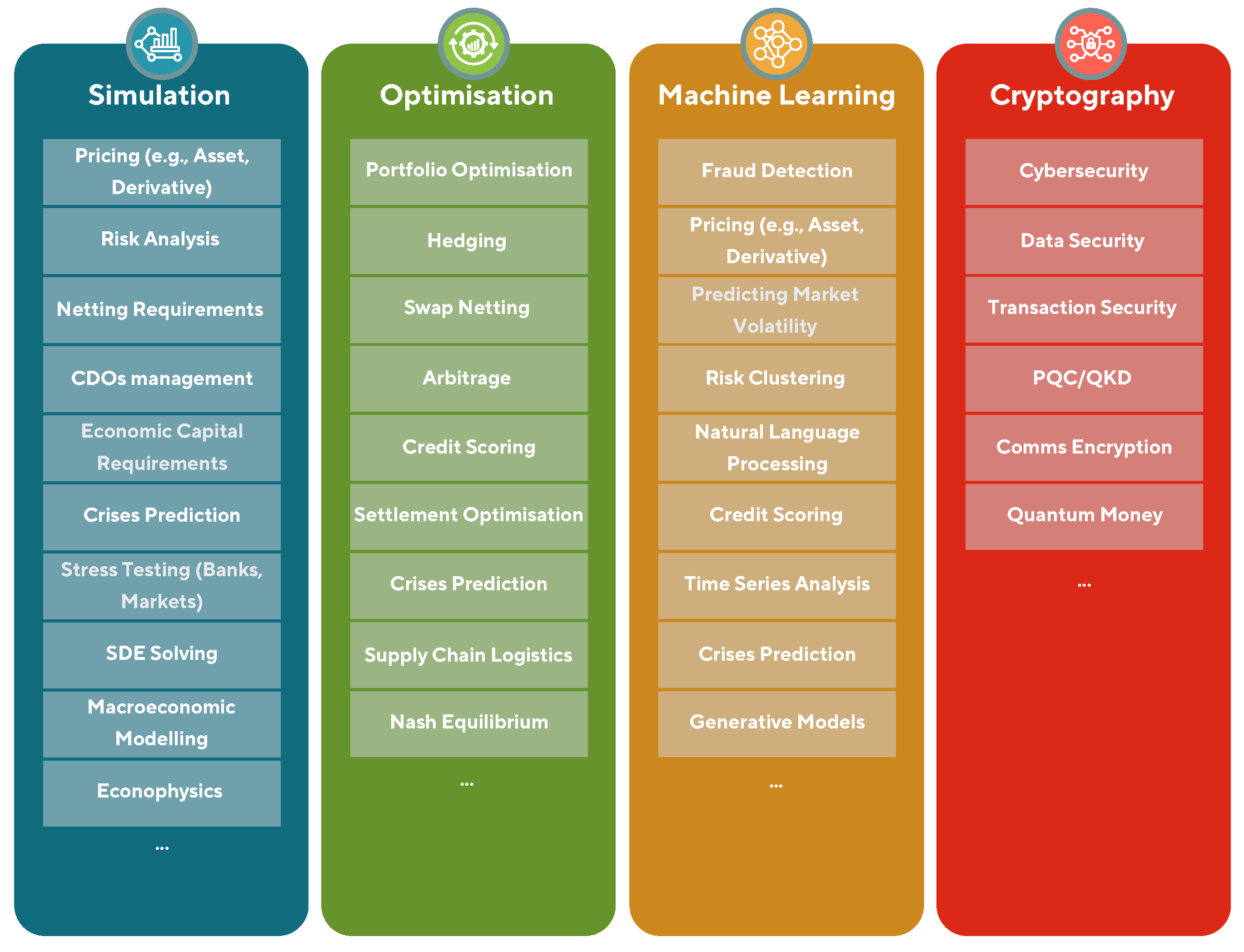
Figure 2.
A sketch of classical and quantum computers’ function in the VQE algorithm. The CPU sets and updates the parameters using an optimiser. The new parameters are used to prepare a quantum state on the QPU which is used to compute the expectation value . Then the CPU takes this output , and based on the energy difference decides to either terminate (convergence at ) or continue loop with new variational parameters .
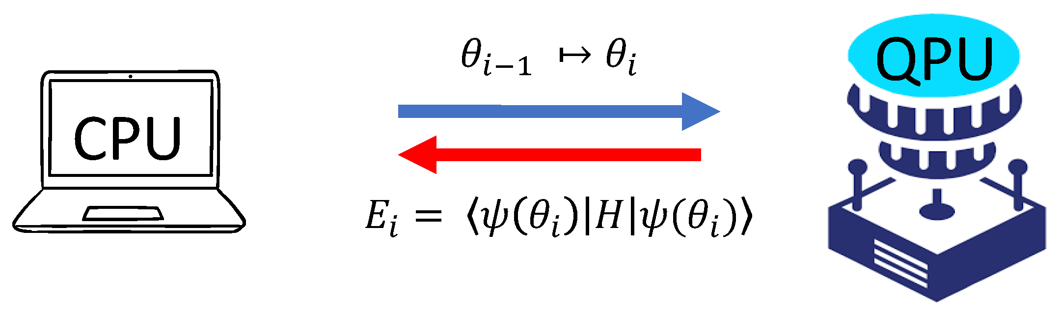
Figure 3.
An overview of the main steps of the Variational Quantum Eigensolver.
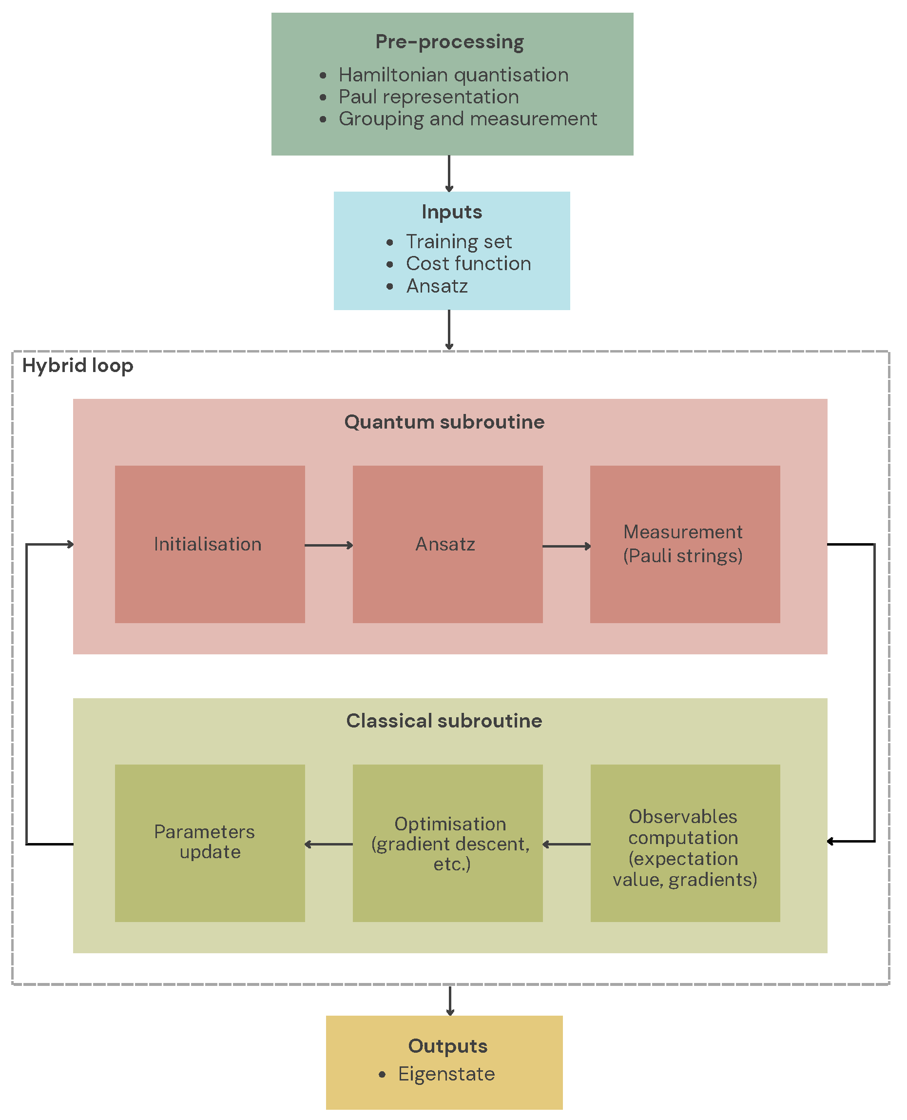
Figure 4.
Example of SVM binary classification. (a) Linearly separable dataset, (b) non-linearly separable case, and (c) the same data transformed into a higher-dimensional feature space using kernel methods, where linear separation becomes possible. Adapted from [301].
Figure 4.
Example of SVM binary classification. (a) Linearly separable dataset, (b) non-linearly separable case, and (c) the same data transformed into a higher-dimensional feature space using kernel methods, where linear separation becomes possible. Adapted from [301].
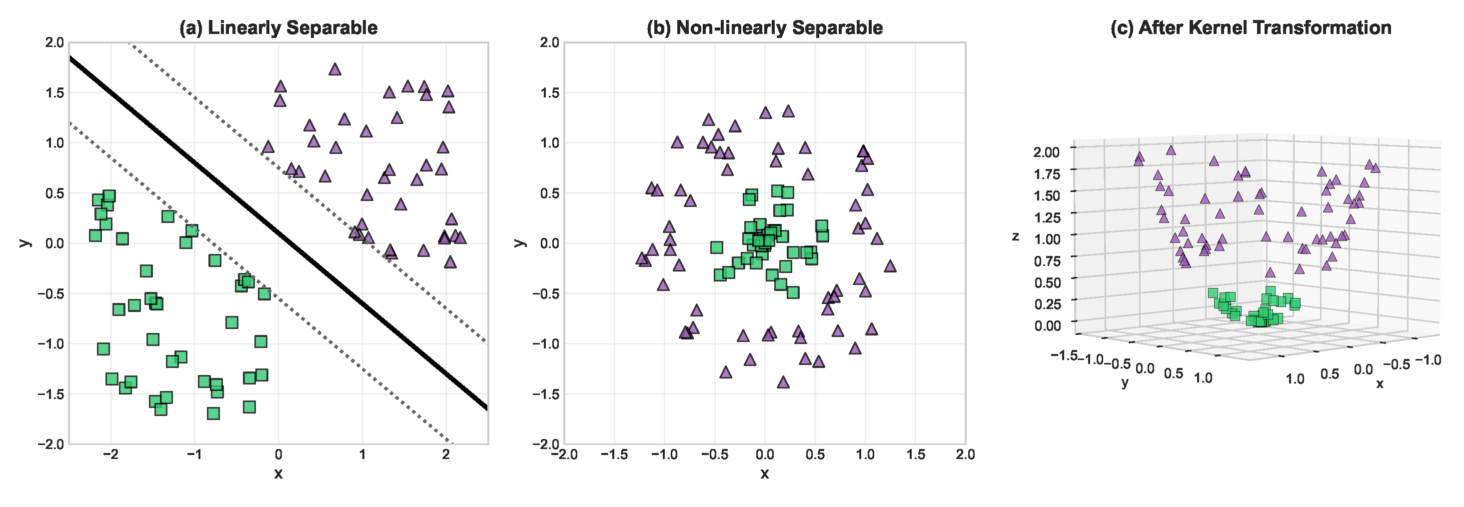
Figure 5.
The DHKX protocol, illustrated with mixing paint, which represents the numbers Alice and Bob send between themselves to arrive at a shared secure key.
Figure 5.
The DHKX protocol, illustrated with mixing paint, which represents the numbers Alice and Bob send between themselves to arrive at a shared secure key.
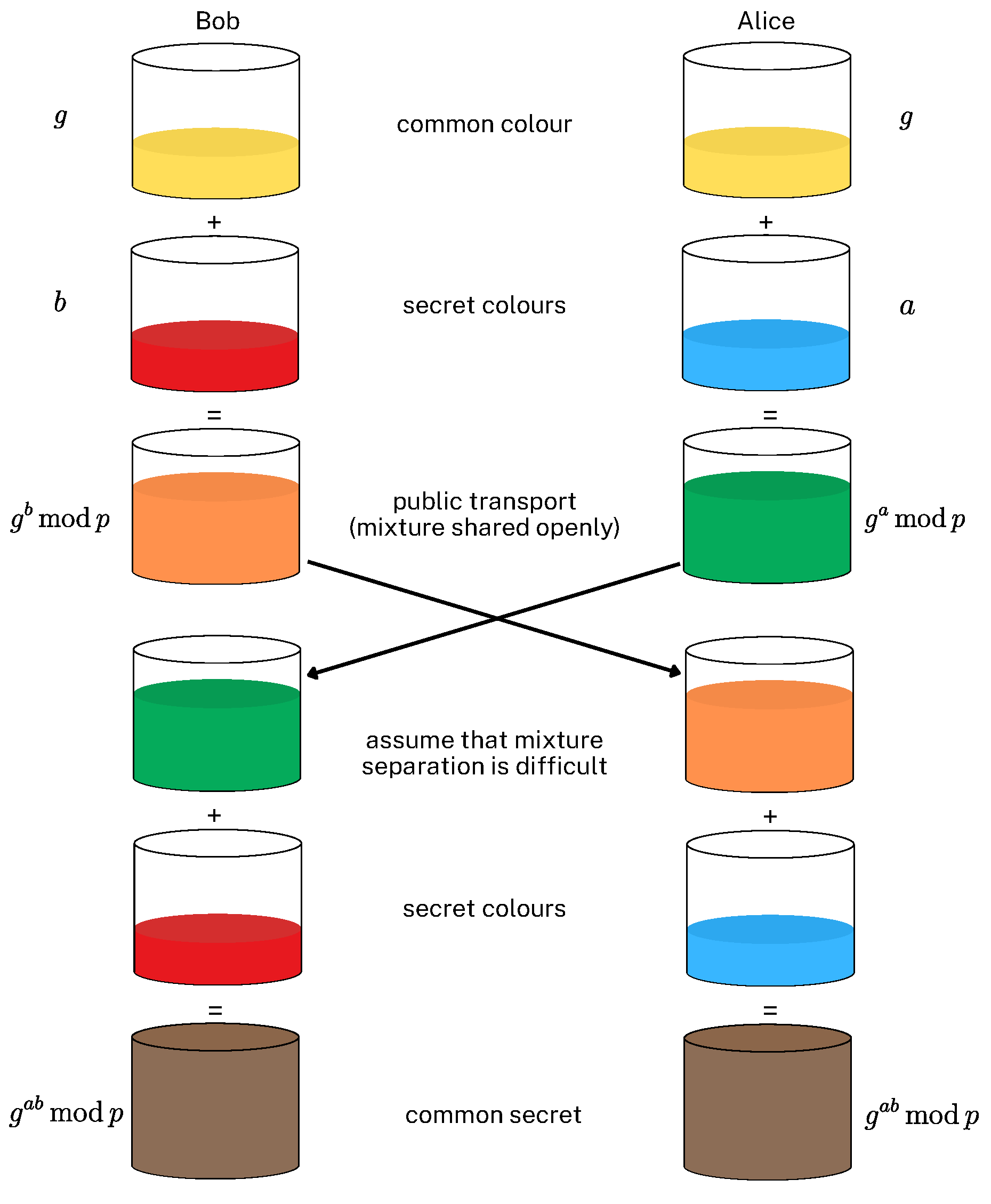
Figure 6.
The results in this section are based on QQ in (a), and the trading toy model (b) for quantum assets. Both figures are adapted based on [608].
Figure 6.
The results in this section are based on QQ in (a), and the trading toy model (b) for quantum assets. Both figures are adapted based on [608].
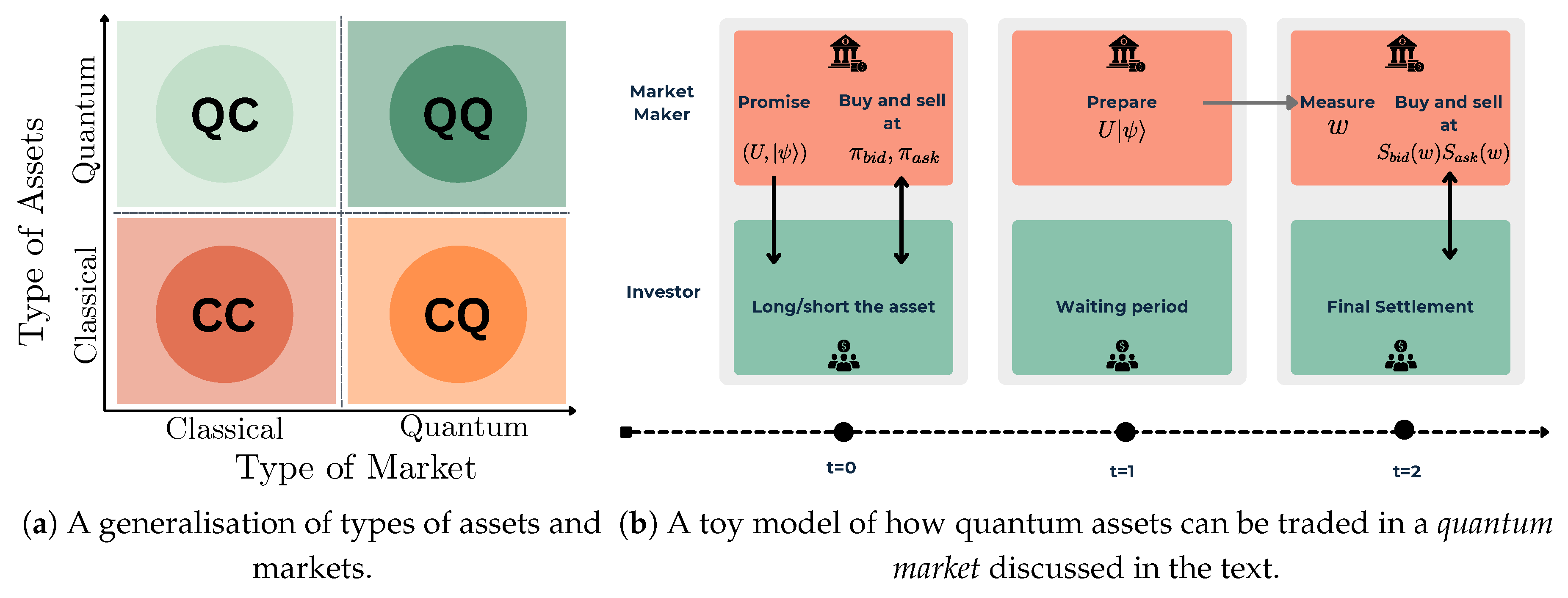
Figure 7.
FIA ETD data of asset class trading volume of futures and options in January 2024 and 2025 [615]. Although there was a decline of nearly 40% from 2024 to 2025, the total volume is still in the order of billions of trades per year, of which more than 80% are based on underlying equity assets.
Figure 8.
An illustrative workflow of option pricing which involves: (1) choosing the type of option, (2) selecting an appropriate model of the underlying assets, and (3) choosing a numerical method for the computation. Quantum algorithms have the potential to improve the efficiency of classical numerical methods.
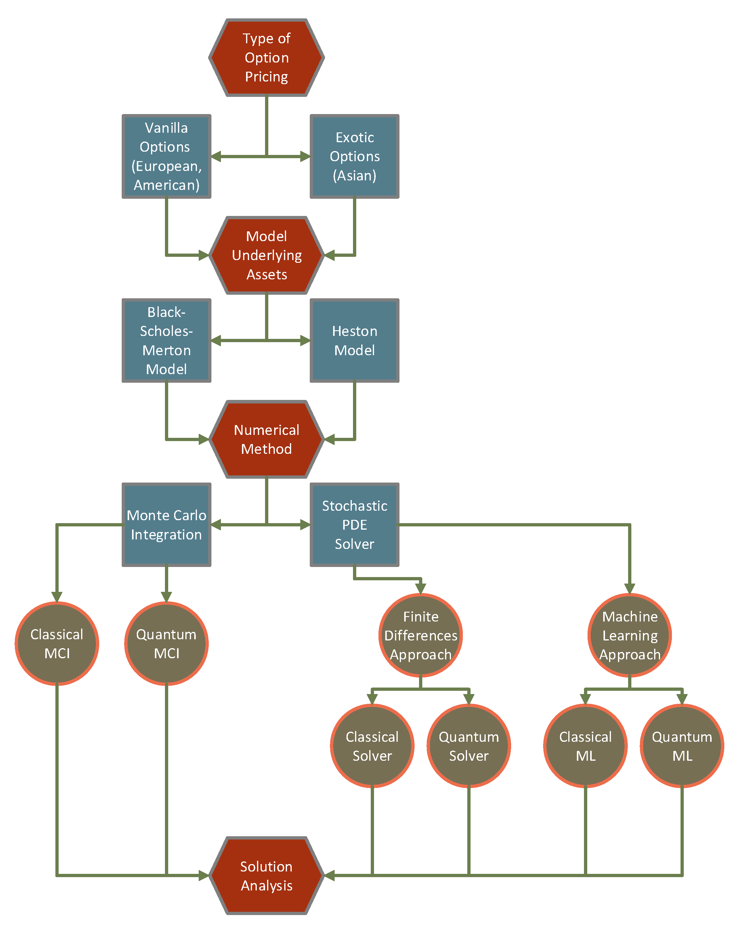
Figure 9.
An example of a random financial network with 4 institutions (blue/top-row) and 5 assets (red/bottom-row).
Figure 9.
An example of a random financial network with 4 institutions (blue/top-row) and 5 assets (red/bottom-row).
Figure 10.
A mapping between use cases and applications for each of the main problem categories in quantum finance and economics.
Figure 10.
A mapping between use cases and applications for each of the main problem categories in quantum finance and economics.
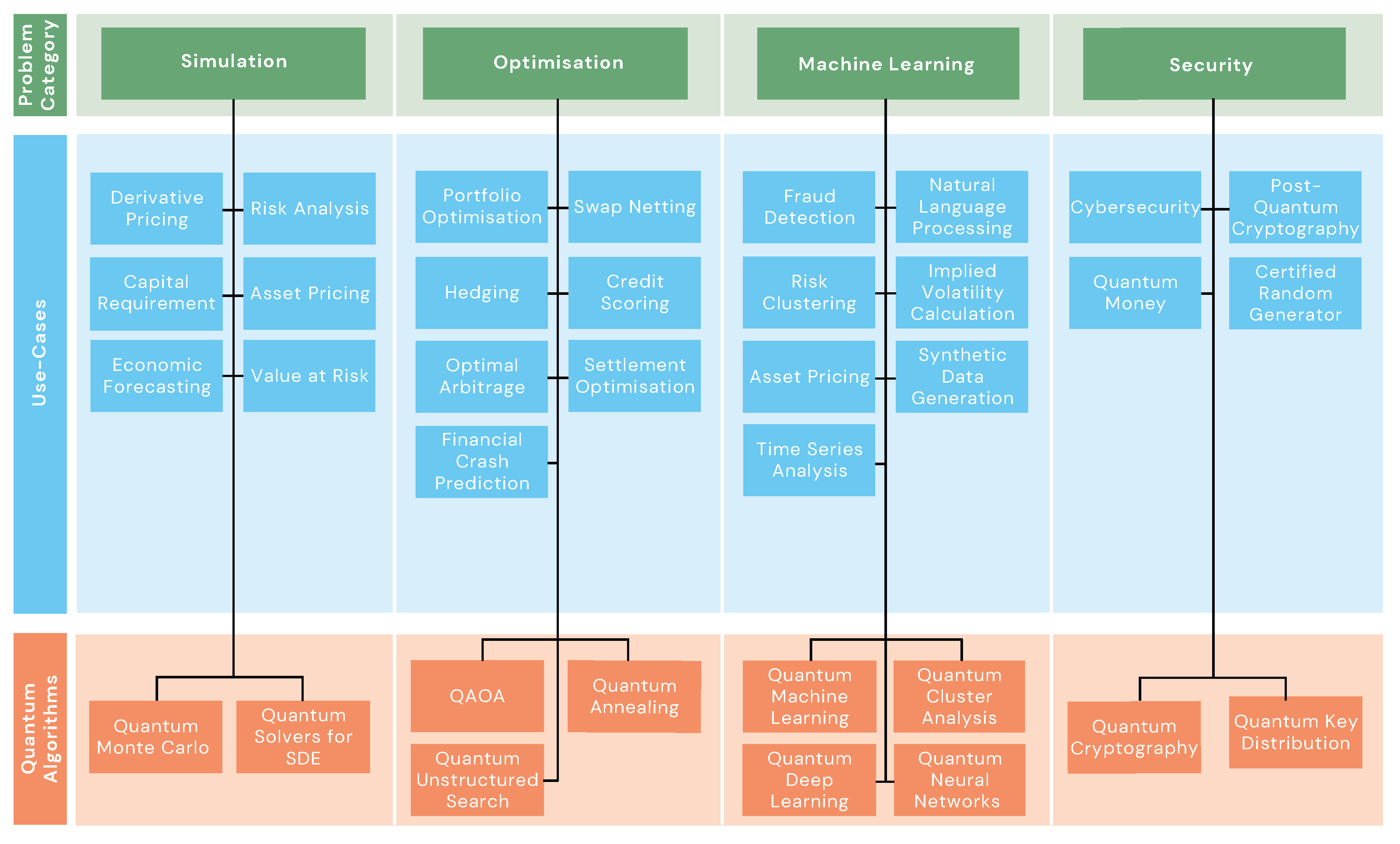

Table 1.
Related survey papers on quantum computing applications in finance.
| Year | First Author | Title of Publication |
| 2019 | Orús [9] | Quantum computing for finance: Overview and prospects |
| 2020 | Egger [23] | Quantum Computing for Finance: State-of-the-Art and Future Prospects |
| 2020 | Alcazar [24] | Classical versus quantum models in Machine Learning: insights from a finance application |
| 2020 | Hull [25,26] | Quantum Technology for Economists |
| 2021 | Pistoia [27] | Quantum Machine Learning for Finance ICCAD Special Session Paper |
| 2022 | García [28] | Systematic Literature Review: Quantum Machine Learning and its applications |
| 2022 | Albareti [29] | A Structured Survey of Quantum Computing for the Financial Industry |
| 2022 | Gómez [31] | A Survey on Quantum Computational Finance for Derivatives Pricing and VaR |
| 2023 | Herman [30] | Quantum computing for finance |
| 2023 | Chang [32] | The Prospects of Quantum Computing for Quantitative Finance and Beyond |
| 2023 | Naik [33] | From Portfolio Optimization to Quantum Blockchain and Security: A Systematic Review of Quantum Computing in Finance |
| 2023 | Saxena [34] | Financial modelling using quantum computing |
| 2024 | Jacquier [35] | Quantum Machine Learning and optimisation in finance |
| 2024 | Claudiu [36] | Enhancing the Financial Sector with Quantum Computing: A Comprehensive Review of Current and Future Applications |
| 2024 | Lu [37] | Quantum financing system: A survey on quantum algorithms, potential scenarios and open research issues |
| 2024 | Atadoga [38] | The Intersection of Artificial Intelligence And Quantum Computing In Financial Markets: A Critical Review |
| 2024 | Gujju [39] | Quantum Machine Learning on near-term quantum devices: Current state of supervised and unsupervised techniques for real-world applications |
| 2024 | Bunescu [40] | Modern finance through quantum computing—A systematic literature review |
| 2024 | Mironowicz [41] | Applications of Quantum Machine Learning for Quantitative Finance |
| 2024 | Auer [22] | Quantum computing and the financial system |
| 2025 | Corli [42] | Quantum Machine Learning algorithms for anomaly detection: A review |
Table 2.
Common notation in quantum computing and analysis of quantum algorithms.
| Symbol | Meaning | Description |
|---|---|---|
| , | Dirac bra-ket notation for a general quantum state and its adjoint, respectively. | A general qubit state: , where . Here, the basis vectors are , |
| Inner product | Measures the overlap or amplitude between two quantum states. | |
| U | Unitary operator | Reversible transformation that preserves norm: . |
| Hamiltonian | Operator that represents the total energy of a quantum system. It determines its time evolution via the unitary . | |
| H | Hadamard gate | Puts a qubit into superposition: . |
| Pauli gates | Single-qubit gates: X (bit flip), Z (phase flip), Y (both flip), I (identity). | |
| , CNOT | Controlled-NOT gate | Two-qubit gate that flips the target if control qubit is . |
| T | T-gate define as | A non-Clifford single-qubit gate that plays two key roles: (i) universality for the set of Clifford gates plus T-gate [44], and (ii) efficient decomposition of Toffoli gates [45] the equivalent of classical gates [46]. |
| ⊗, Tr | Tensor product and Trace | Combines states: . Trace gives the sum of matrix diagonal entries; used in measurement and subsystems. |
| Big-O notation | Describes asymptotic upper bounds on complexity of an algorithm. | |
| Big-Omega notation | Describes asymptotic lower bounds on complexity of an algorithm. | |
| Big-Theta notation | Describes asymptotic average or tight (upper and lower) bounds on the complexity of an algorithm. | |
| meas or M | Measurement | Collapses qubit to classical bit based on amplitude probabilities. |
Table 3.
Comparison of the complexity between various algorithms for the LSP (first two rows) and QLSP. Here, N is the dimension of the system, is the desired precision, s and are the sparsity and condition number of the matrix A, respectively. Note that all the quantum algorithms (except one based on QSVE in the 6th row) for the QLSP have a complexity factor of in terms of the system size.
| Assumption | Algorithm | Complexity |
|---|---|---|
| A is symmetric, s-sparse, and positive definite. | Conjugate Gradient [122] | |
| A can be a dense square matrix | Powers of tensors [123] | with |
| A is s-sparse, Hermitian with singular values | HHL - Hamiltonian simulation with QPE [6] | |
| Same as HHL | Variable-time amplitude amplification [124] | |
| Same as HHL | Fourier or Chebyshev fitting using LCU [125] | |
| A is dense, Hermitian with eigenvalues in | Quantum Singular Value Estimation [126] | |
| A generates Hamiltonian with spectral gap amplification constraints [127] | Adiabatic random method [128] | |
| A general non-Hermitian matrix | Time-optimal adiabatic methods [129] | |
| Same as HHL | Zeno eigenstate filtering [130] | |
| Same as HHL | Quantum discrete adiabatic theorem [131] | |
| Same as HHL | Kernel projection methods [132] |
Table 4.
Examples of how the general asset pricing problem of Equation (133) translates to other pricing problems. Here, is the stock dividend, and other variables are explicitly defined in [181].
| Asset | Price | Payoff |
| Stock | ||
| Return | 1 | |
| Price-dividend ratio | ||
| Excess return | 0 | |
| Managed portfolio | ||
| Moment condition | ||
| One-period bond | 1 | |
| Risk-free rate | 1 | |
| Option | C |
Table 5.
Traditional models: BSM and Heston for the stochastic dynamics of the value of the underlying asset .
Table 5.
Traditional models: BSM and Heston for the stochastic dynamics of the value of the underlying asset .
| BSM | Heston | |
| Assumption | constant volatility | stochastic volatility |
| SDE |
Disclaimer/Publisher’s Note: The statements, opinions and data contained in all publications are solely those of the individual author(s) and contributor(s) and not of MDPI and/or the editor(s). MDPI and/or the editor(s) disclaim responsibility for any injury to people or property resulting from any ideas, methods, instructions or products referred to in the content. |
© 2026 by the authors. Licensee MDPI, Basel, Switzerland. This article is an open access article distributed under the terms and conditions of the Creative Commons Attribution (CC BY) license (http://creativecommons.org/licenses/by/4.0/).
Copyright: This open access article is published under a Creative Commons CC BY 4.0 license, which permit the free download, distribution, and reuse, provided that the author and preprint are cited in any reuse.


