
Submitted:
18 November 2025
Posted:
20 November 2025
You are already at the latest version
Abstract
We derive an explicit analytic expression for the first quantum correction to the second virial coefficient of a $d$-dimensional fluid whose particles interact via the generalized Lennard-Jones $(2n,n)$ potential. By introducing an appropriate change of variable, the correction term is reduced to a single integral that can be evaluated in closed form in terms of parabolic cylinder or generalized Hermite functions. The resulting expression compactly incorporates both dimensionality and stiffness, providing direct access to the low- and high-temperature asymptotic regimes. In the special case of the standard Lennard-Jones fluid ($d=3$, $n=6$), the formula obtained is considerably more compact than previously reported representations based on hypergeometric functions. The knowledge of this correction allows us to determine the first quantum contribution to the Boyle temperature, whose dependence on dimensionality and stiffness is explicitly analyzed. Moreover, the same methodology can be systematically extended to obtain higher-order quantum corrections.
Keywords:
second virial coefficient
; quantum corrections
; generalized Lennard-Jones potential
; semiclassical fluids
; parabolic cylinder functions
1. Introduction
In a semiclassical fluid, the second virial coefficient can be expressed as [1,2,3,4,5,6,7,8]
where
is the classical contribution, and
represents the first quantum correction. In Eqs. (2) and (3), denotes the pair potential, , and is the total solid angle in d dimensions.
The prototypical pair potential in liquid-state theory is the Lennard-Jones (LJ) potential,
where and set the energy and length scales, respectively. The standard LJ (sLJ) fluid corresponds to and , while the generalized Lennard-Jones (gLJ) model allows arbitrary dimensionality d and stiffness parameter . In the limit , the gLJ potential of Eq. (4) approaches the hard-sphere potential.
By introducing the reduced (dimensionless) coefficients
we obtain
where is the reduced temperature.
Several equivalent representations of for the sLJ fluid can be found in the literature (see, for instance, Ref. [8] and references therein). Perhaps the most compact expression—valid for the gLJ fluid—is [9, Sec. 3.7]
where
is the parabolic cylinder function [10]. In Eq. (8), denotes the Heaviside step function.
Naturally, the situation is more involved for the quantum contribution . In a recent work, Zhao et al. [8] derived a linear, second-order homogeneous ordinary differential equation for the sLJ coefficient . From its solution, they obtained
where
2. First Quantum Correction to the Second Virial Coefficient
Our goal is to derive an alternative, more compact expression for in the broader case of the gLJ fluid. We begin by stating the final result:
By introducing the change of variable in Eq. (6b), we obtain
where we have introduced the shorthand notation , . Using the definition of the parabolic cylinder function, Eq. (8), Eq. (13) can be rewritten as
This expression is already quite compact, but it can be further simplified. Iterative application of Eq. (12a) yields
Next, we apply Eq. (12a) to the term , which gives
Substituting this identity into Eq. (14), and returning to the physical variables and , we recover Eq. (11). In terms of the generalized Hermite functions, Eq. (11) can be rewritten as
For the particular case of the sLJ model (, ),
It can be verified that Eq. (18) is equivalent to the combination of Eqs. (9) and (10).
The limits given by Eq. (12c) allow us to determine the low- and high-temperature behaviors of for the gLJ fluid:
In the second equality of Eq. (19), use has been made of the identity .
Interestingly, Eq. (11) simplifies considerably in the case of a two-dimensional fluid (). Using Eq. (12d), we obtain
In this case, the ratio is independent of the stiffness parameter n.
Figure 1 illustrates the temperature dependence of for the two- and three-dimensional gLJ fluids with , 5, 6, 7, 8, and 12. As can be seen, for a given , the reduced first quantum correction increases as the potential becomes stiffer. Moreover, the influence of n is more pronounced at high temperatures than at low temperatures, consistent with the limiting behaviors described by Eq. (19). For the same values of and n, is larger in the two dimensions than in three.
3. First Quantum Correction to the Boyle Temperature
From Eq. (1), the reduced second virial coefficient of the gLJ fluid can be written as
The Boyle temperature, , is defined by the condition . It marks the balance between the attractive and repulsive contributions to the intermolecular potential: the attractive interactions dominate for , whereas the repulsive ones dominate for . In the semiclassical regime, the Boyle temperature can be expanded as
where is the classical Boyle temperature, i.e., the solution of , or equivalently, . By inserting Eq. (22) into Eq. (21), one obtains the first quantum correction to the Boyle temperature,
Thus, one finally obtains
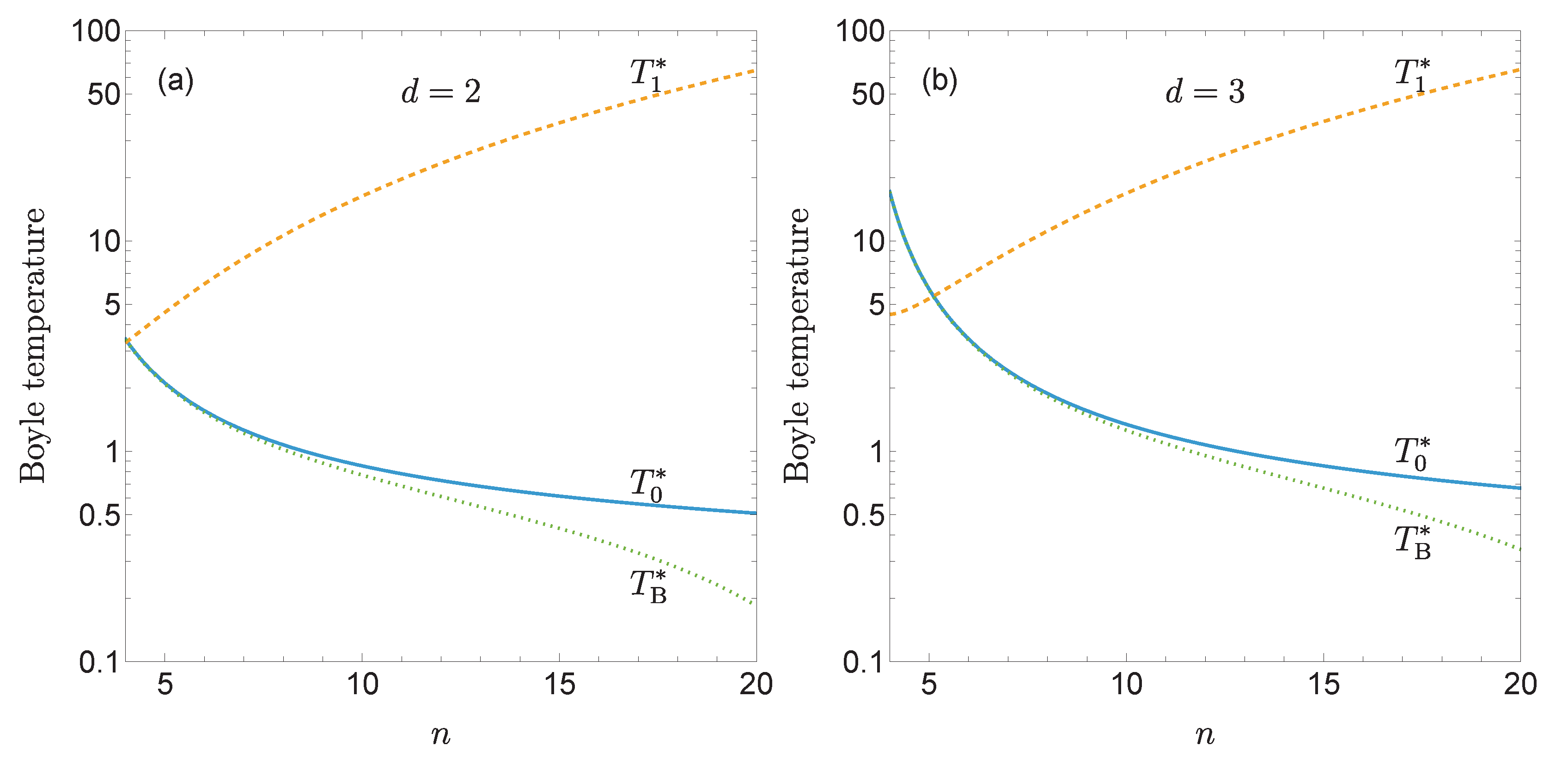
Figure 2 shows and as functions of n for and . While the classical Boyle temperature decreases as the potential becomes stiffer, the first quantum correction increases with n. As a result, quantum effects amplify the decrease of the Boyle temperature with increasing stiffness, as illustrated by the curves representing with . This effect is more pronounced in two-dimensional fluids than in three-dimensional ones.
4. Conclusions
In this paper, we have derived an explicit and compact expression, Eq. (11), for the first quantum correction to the second virial coefficient of a d-dimensional fluid composed of particles interacting through the gLJ potential defined in Eq. (4). As in the classical case, Eq. (8), the first quantum correction has been conveniently expressed in terms of parabolic cylinder functions. For the particular case of the sLJ fluid (, ), the expression obtained here for [see Eq. (18)] is considerably more concise than the combination of Eqs. (9) and (10) reported previously [4,8].
An additional asset of the present results is that they allow one to explore the combined influence of dimensionality and stiffness on the quantum correction . From Eq. (11), it follows that the ratio depends on d and n only through the combination . This implies that, at a given temperature, the value of for a three-dimensional fluid with stiffness n is identical to that of a d-dimensional fluid () with an effective stiffness . In contrast, for two-dimensional fluids, is independent of n and is given by the particularly simple expression of Eq. (17).
The knowledge of has enabled us to derive the first quantum correction to the Boyle temperature [see Eq. (22)]. As illustrated by Figure 1 and Figure 2, the general trend is that the quantum corrections to both the second virial coefficient and the Boyle temperature become more significant as the potential stiffness increases and the system dimensionality decreases.
Although in this work we have focused on the first quantum correction to , the same methodology can be extended to higher-order terms. For example, the general expression for the second-order correction reads [1,2]
Specializing to the gLJ potential, Eq. (4), and introducing the change of variable , one can express in terms of the parabolic cylinder functions , , …, , with . This expression can be further simplified through repeated application of Eq. (12a).
In summary, we have obtained a compact and fully explicit expression for the first quantum correction to the second virial coefficient of a d-dimensional gLJ fluid, expressed in terms of parabolic cylinder or generalized Hermite functions. The formulation unifies the treatment of dimensionality and stiffness, provides analytic access to the limiting behaviors, and naturally yields the quantum correction to the Boyle temperature. Beyond its intrinsic theoretical interest, the approach presented here provides a systematic framework for deriving higher-order quantum corrections of relevance in quantum and semiclassical fluid theory
Author Contributions
Conceptualization, A.S.; methodology, D.P. and A.S.; software, A.S.; validation, D.P. and A.S.; formal analysis, D.P. and A.S.; investigation, D.P. and A.S.; writing—original draft preparation, A.S.; writing—review and editing, D.P. and A.S.; visualization, A.S.; supervision, A.S.; funding acquisition, A.S. All authors have read and agreed to the published version of the manuscript.
Funding
A.S. acknowledges financial support from Grant No. PID2024-156352NB-I00 funded by MCIU/AEI/ 10.13039/501100011033/FEDER, UE and from Grant No. GR24022 funded by the Junta de Extremadura (Spain) and by European Regional Development Fund (ERDF) “A way of making Europe.”
Institutional Review Board Statement
Not applicable.
Data Availability Statement
The raw data supporting the conclusions of this article will be made available by the authors on request.
Conflicts of Interest
The authors declare no conflicts of interest.
Abbreviations
The following abbreviations are used in this manuscript:
| gLJ | generalized Lennard-Jones |
| LJ | Lennard-Jones |
| sLJ | standard Lennard-Jones |
References
- Kihara, T. Virial Coefficients and Models of Molecules in Gases. B. Rev. Mod. Phys. 1955, 27, 412–423. [Google Scholar] [CrossRef]
- Kihara, T.; Midzuno, Y.; Shizume, T. Virial Coefficients and Intermolecular Potential of Helium. J. Phys. Soc. Jpn. 1955, 10, 249–255. [Google Scholar] [CrossRef]
- DeWitt, H.E. Analytic Properties of the Quantum Corrections to the Second Virial Coefficient. J. Math. Phys. 1962, 3, 1003–1016. [Google Scholar] [CrossRef]
- Michels, H.H. Low-Temperature Quantum Corrections to the Second Virial Coefficient. Phys. Fluids 1966, 9, 1352–1358. [Google Scholar] [CrossRef]
- Boyd, M.E.; Larsen, S.Y.; Kilpatrick, J.E. Quantum Mechanical Second Virial Coefficient of a Lennard-Jones Gas. Helium. J. Chem. Phys. 1969, 50, 4034–4055. [Google Scholar] [CrossRef]
- Boyd, M.E. Quantum Corrections to the Second Virial Coefficientfor the Lennard-Jones (m-6) Potential. J. Res. Natl. Bur. Stand. A Phys. Chem. 1971, 75A, 57–95. [Google Scholar] [CrossRef] [PubMed]
- Mamedov, B.A.; Somuncu, E. Evaluation of Quantum Corrections to Second Virial Coefficient with Lennard-Jones (12-6) Potential. J. Phys.: Conf. Ser. 2016, 766, 012010. [Google Scholar] [CrossRef]
- Zhao, Z.; González-Calderón, A.; Perera-Burgos, J.A.; Estrada, A.; Hernández-Anguiano, H.; Martínez-Lázaro, C.; Li, Y. Exact ODE Framework for Classical and Quantum Correctionsfor the Lennard-Jones Second Virial Coefficient. Entropy 2025, 27, 1059. [Google Scholar] [CrossRef] [PubMed]
- Santos, A. A Concise Course on the Theory of Classical Liquids. Basics and Selected Topics; Vol. 923, Lecture Notes in Physics, Springer: New York, 2016. [Google Scholar]
- NIST Digital Library of Mathematical Functions. https://dlmf.nist.gov/, Release 1.2.4 of 2025-03-15. F. W. J. Olver, A. B. Olde Daalhuis, D. W. Lozier, B. I. Schneider, R. F. Boisvert, C. W. Clark, B. R. Miller, B. V. Saunders, H. S. Cohl, and M. A. McClain, eds.
Figure 1.
Reduced first quantum correction to the second virial coefficient, as given by Eq. (11), for the gLJ fluid with (a) and (b) . The curves correspond, from bottom to top, to stiffness parameters , 5, 6, 7, 8, and 12.
Figure 1.
Reduced first quantum correction to the second virial coefficient, as given by Eq. (11), for the gLJ fluid with (a) and (b) . The curves correspond, from bottom to top, to stiffness parameters , 5, 6, 7, 8, and 12.
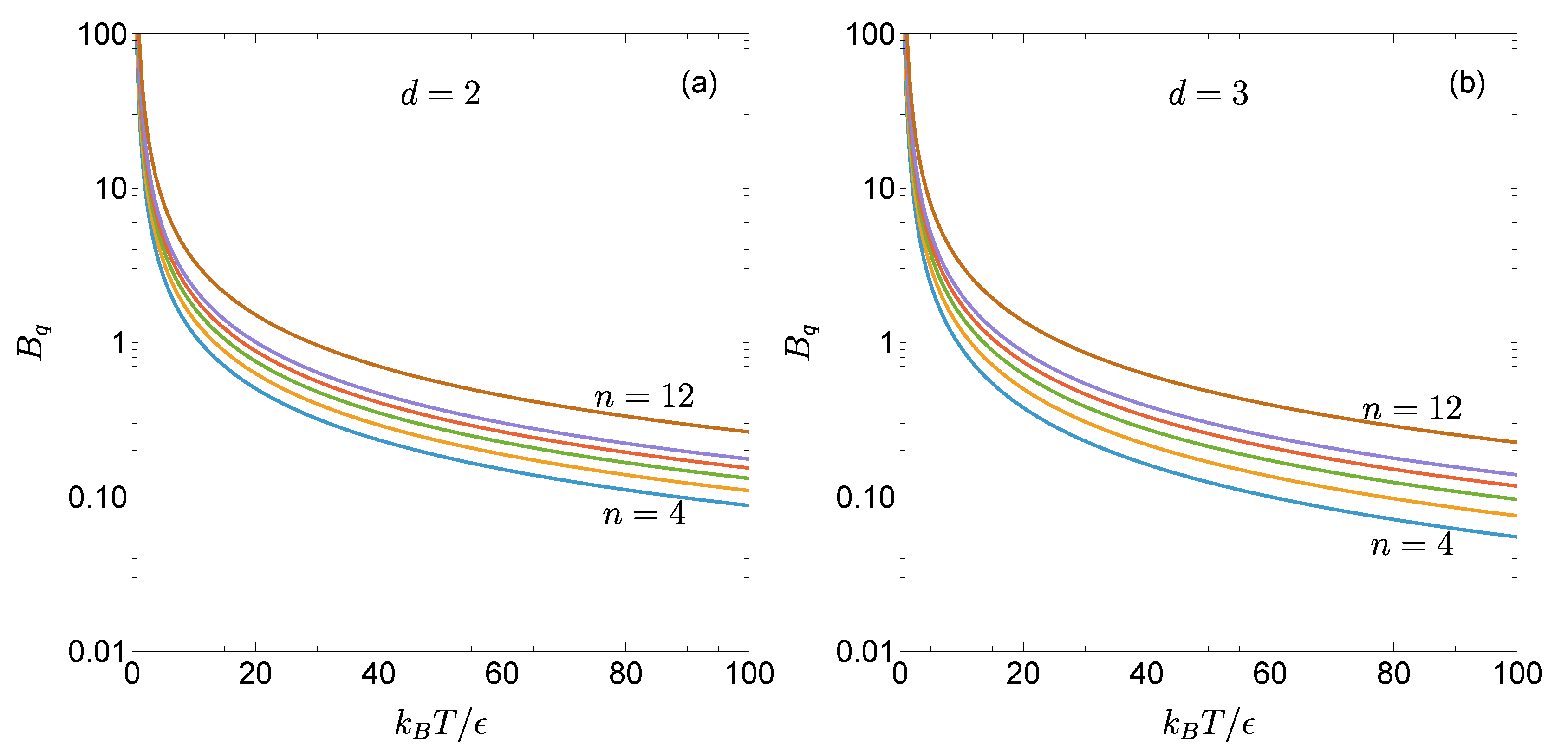
Figure 2.
Classical Boyle temperature (solid lines) and its first quantum correction (dashed lines) as functions of the stiffness parameter n for the gLJ fluid with (a) and (b) . The dotted lines represent the quantum-corrected Boyle temperature , obtained Eq. (19) with .
Figure 2.
Classical Boyle temperature (solid lines) and its first quantum correction (dashed lines) as functions of the stiffness parameter n for the gLJ fluid with (a) and (b) . The dotted lines represent the quantum-corrected Boyle temperature , obtained Eq. (19) with .
Disclaimer/Publisher’s Note: The statements, opinions and data contained in all publications are solely those of the individual author(s) and contributor(s) and not of MDPI and/or the editor(s). MDPI and/or the editor(s) disclaim responsibility for any injury to people or property resulting from any ideas, methods, instructions or products referred to in the content. |
© 2025 by the authors. Licensee MDPI, Basel, Switzerland. This article is an open access article distributed under the terms and conditions of the Creative Commons Attribution (CC BY) license (http://creativecommons.org/licenses/by/4.0/).
Copyright: This open access article is published under a Creative Commons CC BY 4.0 license, which permit the free download, distribution, and reuse, provided that the author and preprint are cited in any reuse.


