
Submitted:
17 November 2025
Posted:
18 November 2025
You are already at the latest version
Abstract
Unmanned airships are highly sensitive to parametric uncertainty, persistent wind disturbances, and sensor noise, all of which compromise reliable path following. Classical control schemes often suffer from chattering and fail to handle index discontinuities on closed-loop paths due to the lack of mechanisms, and cannot simultaneously provide formal guarantees on state constraint satisfaction. We address these challenges by developing a unified, constraint-aware guidance and control framework for path following in uncertain environments. The architecture integrates an extended state observer (ESO) to estimate and compensate lumped disturbances, a barrier Lyapunov function (BLF) to enforce state constraints on tracking errors, and a Super-Twisting Terminal Sliding Mode (ST-TSMC) control law to achieve finite-time convergence with continuous, low-chatter control inputs. A constructive Lyapunov-based synthesis is presented to derive the control law and to prove that all tracking errors remain within prescribed error bounds. At the guidance level, a nonlinear curvature-aware line-of-sight (CALOS) strategy with an index-increment mechanism mitigates jump phenomena at loop-closure and segment-transition points on closed yet discontinuous paths. The overall framework is evaluated against representative baseline methods under combined wind and parametric perturbations. Numerical results indicate improved path-following accuracy, smoother control signals, and strict enforcement of state constraints, yielding a disturbance-resilient path-following solution for the cruise of an unmanned airship.
Keywords:
unmanned airship
; path-following
; barrier lyapunov function
; extended state observer
; super-twisting terminal sliding mode control
; nonlinear curvature-aware line-of-sight guidance
; jump suppression
1. Introduction
Unmanned airships are experiencing a resurgence in strategic interest for applications demanding long-endurance and high-altitude station-keeping, such as persistent surveillance, atmospheric sensing, and serving as high-altitude pseudo-satellites (HAPS) for telecommunications [1,2]. Their inherent energy efficiency and substantial payload capacity make them particularly suited for missions impractical for conventional fixed-wing or rotary-wing UAVs [3]. However, realizing this potential is contingent upon developing highly reliable autonomous navigation systems. A cornerstone of this autonomy is path-following control, which requires the airship to converge to and maintain a predefined geometric path in the presence of significant and persistent operational challenges [4].
The control of unmanned airships is a challenging problem, fundamentally complicated by a confluence of several interacting factors. One arises from the airship’s internal dynamics, which are characterized by large inertia, low damping, and highly coupled nonlinear behavior, rendering the vehicle inherently sluggish and difficult to stabilize [5]. This inherent dynamic challenge is exacerbated by the operational environment, as operating at high altitudes exposes the vehicle to persistent and intense wind fields, whose wind velocity can be a significant fraction of the airship’s airspeed. Consequently, this elevates wind from a disturbance to a dominant and mission-critical factor demanding robust compensation [6]. Compounding these challenges, many missions, such as area surveillance, require the airship to follow closed-loop and repetitive trajectories (e.g., racetrack patterns), often while satisfying strict state constraints on tracking error to ensure safety or sensor coverage. These paths introduce topological challenges for guidance systems, such as reference discontinuity, which are not encountered in simple point-to-point navigation [7,8]. Addressing these multifaceted challenges calls for an integrated guidance and control architecture that provides robustness, smooth actuation, topological consistency, and explicit constraint handling.
The LOS guidance law remains a well-established and widely adopted method, valued for its geometric clarity and low computational overhead [9]. It operates by directing the vehicle towards a virtual target or look-ahead point situated on the desired path. However, classical LOS guidance with a fixed look-ahead distance suffers from an inherent trade-off: a small distance yields aggressive tracking but risks oscillations, while a large distance ensures smoothness at the cost of sluggish response. More importantly, the LOS guidance law is susceptible to steady-state cross-track errors when subjected to persistent lateral disturbances, such as crosswind, regardless of whether the look-ahead distance is small or large [10].
Several extensions of the LOS framework have been developed to improve robustness and tracking accuracy. Integral LOS (ILOS) augments the classical law with an integral term that compensates for constant environmental forces, thereby removing steady-state cross-track errors [11,12]. Subsequent work has introduced adaptive LOS schemes in which the look-ahead distance is adjusted online based on the cross-track error [13]. Although these approaches improve tracking performance on open or piece-wise continuous paths, they share a common and unaddressed limitation that they fail to handle the topological discontinuity inherent in closed-loop trajectories. When the look-ahead point crosses the path’s seam, either at the closure point of a loop (e.g., from the end waypoint back to the start) or at a segment transition (e.g., from a straight section into a turning arc), the path index undergoes an abrupt jump. This discrete index-jump phenomenon causes a discontinuous change in the commanded heading, which can result in control signal saturation and degraded tracking performance, an important concern for persistent loitering missions [14].
At the control layer, Sliding Mode Control (SMC) has been extensively studied for its robustness against matched uncertainties and external disturbances [15]. Its practical application, however, is often hindered by the chattering phenomenon—high-frequency oscillations in the control signal caused by the discontinuous switching law, which may excite unmodeled dynamics and accelerate actuator wear [16,17]. Research to mitigate this issue has primarily followed two paths. The first involves higher-order SMC methods, notably the Super-Twisting Algorithm (STA) [18,19]. By shifting the discontinuity to a higher derivative of the control signal, STA generates a continuous control action effectively suppressing chattering while preserving the finite-time convergence and robustness properties of conventional SMC [20]. The second path aims to enhance convergence speed through TSMC and its nonsingular variants [21]. Unlike conventional SMC, which offers asymptotic stability, TSMC ensures finite-time convergence of the system states, a property often required in fast-response applications [22]. Although the combination of STA and TSMC provides a practical means for achieving low-chatter, finite-time control [23], these methods remain fundamentally reactive. Their efficacy relies on control gains being large enough to dominate the worst-case disturbance bound [24]. For an airship facing large and sustained wind forces, this can result in excessive control effort and may not be the most efficient strategy. These considerations indicate the need for a proactive mechanism capable of estimating and compensating for the dominant portion of the disturbance, thereby reducing the reliance on high-gain robust control.
To enable proactive disturbance compensation, the ESO has emerged as a compelling paradigm [25]. The core concept of an ESO is to aggregate all sources of uncertainty—including external disturbances, unmodeled dynamics, and parametric variations—into a single total disturbance variable [26]. This augmented variable is then treated as an extended state of the system, which the observer estimates in real-time. The notable advantage of the ESO is its weak dependence on detailed system modeling. The ESO requires only coarse structural knowledge of the system’s mathematical model while providing a direct estimate of the total disturbance, which can then be actively compensated in the control loop. These ESO-based designs have been applied across various aerospace platforms, where they have demonstrated improved disturbance rejection and robustness [27].
Despite these individual advances, an important gap remains in integrating these developments into a cohesive framework. Advanced guidance laws, finite-time robust controllers, and disturbance observers have been developed largely as standalone components, and a framework that integrates all three in a unified manner is still lacking. In addition, existing approaches rarely offer formal guarantees on state-constraint bounds satisfaction—such as bounds on tracking error—which are essential for safe operation near obstacles and for maintaining sensor coverage[28,29]. Achieving such integration is nontrivial, as it requires ensuring the stability of a tightly coupled system in which the observer, guidance law, and controller interact dynamically while state constraint bounds must be enforced without relying on excessively high feedback gains.
To address the aforementioned limitations and bridge the identified research gaps, this paper develops a unified guidance and control framework designed to enhance disturbance resilience for unmanned airships executing closed-loop path following missions in uncertain environments. The main contributions of this work are summarized as follows:
- A Curvature-Aware Adaptive LOS Guidance Law: A novel nonlinear LOS guidance law is proposed that dynamically adapts the look-ahead distance based on both local path curvature and cross-track error. This strategy is coupled with an index-increment mechanism that explicitly suppresses the index-jump phenomenon, guaranteeing a smooth and continuous LOS angle command even across the seam of closed-loop trajectories.
- A Unified guidance and control Synthesis with BLF Constraint Guarantee: We develop a unified guidance and control synthesis that rigorously enforces state constraints. A BLF is constructed on the LOS heading error, guaranteeing that this guidance error remains within predefined bounds for all time, thus ensuring stable and predictable controller behavior.
- A Finite-Time, Disturbance-Rejecting ST-TSMC Law: A robust inner-loop controller is developed by integrating an ESO with an ST-TSMC law. The ESO estimates and compensates for lumped physical disturbances and complex kinematic disturbances arising from the LOS geometry. The ST-TSMC law then drives the yaw-rate tracking error to a small residual set in finite time, ensuring chattering-free, robust tracking of the BLF-constrained guidance command.
The remainder of this paper is organized as follows. Section 2 details the airship dynamic model and formulates the path-following control problem. Section 3 presents the geometric representation of the reference path and derives the associated error kinematics. Section 4 constructively derives the integrated guidance and control framework, detailing the ESO, the BLF-SMC synthesis, and the guidance law. Section 5 presents the formal stability analysis, culminating in the unified stability theorem. Section 6 reports simulation studies—together with comparative and robustness evaluations—that assess the performance of the proposed framework. Finally, Section 7 concludes the paper and discusses potential avenues for future research.
2. System Modeling and Problem Formulation
The unmanned airship considered in this study adopts a conventional ellipsoidal envelope filled with helium, which provides the buoyant lift required to sustain flight. The gondola, mounted beneath the envelope, houses the avionics and power systems. Two propellers, symmetrically installed on both sides of the gondola, deliver the main propulsion forces, while the rudder mounted at the empennage surface generates the yaw control moment. The general configuration and coordinate frames for the airship are illustrated schematically in Figure 1.
To describe the planar motion of the airship, two coordinate frames are defined. The Earth-Fixed Reference Frame (ERF), denoted as , is fixed to the ground, with the -axis pointing north and the -axis pointing east. The Body-Fixed Reference Frame (BRF), denoted as , is rigidly attached to the airship with its origin O located at the center of volume (CV). The x-axis is directed forward along the airship’s longitudinal axis toward the nose, while the y-axis is perpendicular to the x-axis and points laterally to the right. The airship’s attitude is characterized by the yaw angle , which specifies the orientation of the BRF relative to the ERF. The attitude of the airship is characterized by the yaw angle , which defines the orientation of the BRF relative to the ERF.
2.1. Kinematic Model
Assuming that the airship behaves as a rigid body and that the motion is restricted to the horizontal plane neglecting pitch and roll dynamics, the kinematic relationship between the position and velocity of the airship in the two coordinate frames can be written as
where represents the position vector of the airship’s Center of Volume (CV) in the ERF, and denotes the surge and sway velocities in the BRF. The transformation matrix captures the geometric coupling introduced by the yaw orientation.
2.2. Dynamic Model
The dynamic behavior of the airship in the horizontal plane can be described by a set of coupled nonlinear equations that capture both translational and rotational motions. These two components are inherently interconnected, since inertial and aerodynamic couplings arise naturally from the vehicle’s geometry and its underactuated configuration.
The translational dynamic component, which describes the surge–sway motion of the airship in the BRF, is dynamically coupled with the yaw behavior and can be expressed in a compact matrix form as
where and are the effective mass terms that incorporate the added-mass effects in the surge and sway directions, respectively; and are the corresponding hydrodynamic damping coefficients; and denotes the total thrust produced by the propellers. The lumped uncertainties and include unmodeled nonlinearities, parametric perturbations, and exogenous disturbances.
The rotational dynamic component, which is dynamically coupled with the translational motion and governs the yaw dynamics, is formulated as:
where and represent the yaw angle and yaw rate, respectively. The matrices and denote the rotational subsystem’s effective inertia and cross-inertial coupling matrix. The physical parameters and quantify the inertial coupling from the translational dynamics and the hydrodynamic yaw damping, respectively. The inputs to the rotational subsystem consist of the control torque , generated by the rudder, and the lumped disturbance , which aggregates all unmodeled dynamics, parametric uncertainties, and external wind effects.
The adopted 3-DOF formulation provides a concise yet sufficient representation of the dominant horizontal-plane dynamics of the airship. By decoupling the vertical motion—which can be independently governed through buoyancy modulation or pitch control—the model preserves essential dynamic characteristics while enabling tractable analysis within the planar domain. Nevertheless, the airship remains an intrinsically underactuated system, featuring three motion states but only two control inputs . Such structural underactuation inherently couples the surge, sway, and yaw dynamics in a nonlinear manner, thereby imposing nontrivial challenges for subsequent controller design and stability analysis.
2.3. Disturbance and Uncertainty Formulation
In realistic flight conditions, the airship is inevitably influenced by environmental factors such as wind, turbulence, and atmospheric pressure variations. Among these, crosswind effects play a particularly dominant role in altering both the translational and rotational responses of the vehicle. To account for these effects, a lumped disturbance vector is introduced to encapsulate unmodeled dynamics, parametric uncertainties, and wind-induced forces and moments. Assuming a mean wind speed acting from direction , the equivalent disturbance components expressed in the BRF are given by
where denote the aerodynamic moment arms measured from the airship’s center of volume (CV) to the aerodynamic center. These relationships effectively capture the coupling between translational and rotational disturbances caused by the lateral wind field.
where ()denotes the unmodeled coupling effects between pitch and roll dynamics, and represent parameter uncertainties associated with the aerodynamic and added-mass effects, and () corresponds to the wind-induced forces and moment described in Eq. (4).
Assumption 1: It is assumed that the overall lumped disturbances are bounded by finite but unknown constants, i.e., (), where and denotes the unknown finite upper bound of the ith lumped disturbance. This mild assumption is standard in nonlinear airship and marine vehicle modeling and provides a foundation for the design of robust control laws that guarantee stability without requiring explicit disturbance estimation.
2.4. Control Objectives
Consider the unmanned airship system governed by the kinematic and dynamic models (1)–(3), subject to the lumped disturbances defined in Eq. (5) and bounded according to Assumption 1. Building upon the path-following error dynamics developed in Section 3, the main objective of this work is to design a robust, finite-time, and constraint-aware control framework that ensures constraint satisfaction and closed-loop stability even in the presence of input saturation. Specifically, the proposed control framework aims to synthesize the desired commanded control input , such that the following control objectives are achieved simultaneously:
-
Finite-time practical convergence. There exist a finite time and nonnegative radii and such that, for all ,In the absence of disturbances, the convergence is exact, corresponding to .
-
Prescribed output constraints. Let be continuously differentiable, time-varying constraint bounds. Define the time-varying safe setConstraint satisfaction is achieved by establishing the forward invariance of .
- Input saturation handling. Let denote the commanded input, while represents the actuator-constrained input satisfying . The actuator nonlinearity is captured through the saturation mappingwhere , and closed-loop stability as well as performance robustness must be preserved in the presence of this nonlinear saturation behavior, potentially requiring integral anti-windup compensation.
3. Path Geometry and Guidance Law Formulation
To facilitate the subsequent development of the guidance and control laws, the reference trajectory is parameterized by its arc length as , where s denotes the arc-length coordinate along the path. The corresponding Frenet frame is defined by the unit tangent and normal vectors and , respectively, while the curvature satisfies the Frenet–Serret relation . The closest-point projection of the vehicle position onto identifies the arc-length parameter associated with the geometrically nearest point on the path. The effective path coordinate used for guidance is then given by , where denotes the local arc-length offset accounting for the displacement between the projection point and the look-ahead location along the curve.
The path-following objective is defined relative to the reference curve . The cross-track error denotes the perpendicular distance between the airship’s position and the closest point on , , and corresponds to the lateral component of expressed in the Frenet frame at :
where denotes the tangent orientation of the reference path at . The evolution of this geometric error follows directly from the Frenet–Serret kinematics [30,31]:
where denote the body-fixed surge and sway velocities, respectively. Defining the relative heading , the kinematic relation (10) simplifies to:
Eq. (11) shows that the cross-track error is an unactuated state whose evolution is dictated solely by the relative heading and the lateral velocity v. As a result, can only be regulated indirectly by appropriately shaping the dynamics of through the heading reference , thereby necessitating a guidance law that ensures its convergence to zero.
3.1. Line-of-Sight (LOS) Guidance Formulation
The kinematic relation in (11) shows that the cross-track error can only be influenced indirectly through the heading . To generate a suitable reference for , a Line-of-Sight (LOS) guidance law is adopted. The method constructs an instantaneous virtual target, or look-ahead point , located on the reference path . The relative position vector from the airship’s current location to this look-ahead point determines the LOS angle :
With formulation (12), regulation of the cross-track error is achieved indirectly by steering the airship’s heading toward the time-varying LOS reference . The closed-loop characteristics of this indirect mechanism depend on the specification of the look-ahead point , addressed in the following discussion.
The selection of is determined by the adaptive look-ahead distance . A fixed yields an inherent trade-off: large values promote smooth control action but degrade tracking accuracy in high-curvature segments, whereas small values enhance tracking responsiveness at the expense of increased control sensitivity and potential oscillations [30]. To balance these competing effects, is adjusted online. The look-ahead point is defined as the point on that lies an arc length of ahead of the closest path point . The adaptation mechanism regulates through two geometric error indicators. First, the distance is modulated inversely with the local curvature via , reducing in high-curvature regions to maintain tracking fidelity and prevent premature shortcutting of the path. Second, the distance is scaled by the lateral deviation through , which decreases when the vehicle is substantially displaced from the path, thereby promoting a more direct intercept trajectory and improving convergence. These complementary effects are combined into a single, bounded adaptation law:
where and specify the admissible interval for , ensuring compliance with physical limitations and preserving closed-loop stability.
A practical difficulty emerges when applying the guidance logic in Section 3.1 to closed-loop trajectories. Let denote the discrete path index of the look-ahead point at sampling instant k. As the vehicle approaches the path seam corresponding to the index wrap-around, a direct computation of may cause to change discontinuously. Such discontinuities produce abrupt variations in in Eq. (12), thereby introducing undesirable transients into the closed-loop system. To preserve reference continuity, an incremental index–update mechanism is employed in place of a fully recomputed index. Let denote the naively computed index, which may contain a discontinuous jump. The raw incremental change relative to the previous index is:
The raw increment Eq. (14) is subsequently bounded by the admissible rate limit , defined as the maximum allowable index variation over a sampling interval :
The update of the look-ahead index is governed solely by the bounded, rate-limited increment:
3.2. Guidance-Control Error Kinematics
The guidance law in Section 3.1 generates the continuously varying LOS reference in Eq. (12). Accordingly, the control design focuses on regulating the LOS heading error , defined as the angular discrepancy between the vehicle’s heading and the LOS direction:
where denotes the instantaneous angular deviation between the airship’s heading and the virtual target direction. The connection between this kinematic quantity and the dynamic control input, namely the yaw rate r, follows from its time derivative. Differentiating Eq. (17) gives:
Substituting the yaw–rate relation into (18) yields the kinematic expression for the LOS heading error:
The kinematic relation in Eq. (19) provides link between the LOS error dynamics and the control input, reducing the path-following task to the stabilization of a perturbed first-order integrator in the variable r. The LOS rate constitutes a time-varying kinematic disturbance whose value depends not only on the vehicle’s translational velocity but also on the motion of the look-ahead point , the latter being dictated by the adaptive guidance law in Eq. (13).
4. Control Design
To address the challenges of uncertainty and disturbance formulated in the previous section, a hierarchical integrated guidance and control framework is proposed, as illustrated in the framework in Figure 2. The architecture is holistically designed to provide a robust solution by systematically decomposing the path-following task. It is composed of three primary, synergistic components: (1) an ESO to estimate and actively compensate for lumped disturbances in real time, (2) a nonlinear, curvature-aware guidance law to generate robust and continuous desired state commands, and (3) a STS-ATSMC to ensure fast and smooth error convergence of the inner control loops. Each component is detailed in the following subsections.
4.1. Inner-Loop Dynamics and Disturbance Estimation
The control architecture adopts a cascaded structure, in which the inner loop regulates the yaw–rate dynamics, whereas the outer loop governs the path–following kinematics. To ensure reliable tracking of the desired yaw–rate command under parametric uncertainties and external disturbances, we examine the rotational dynamics. From (3), the yaw dynamics are expressed as
Eq.(20) can be reformulated into an affine control form:
where denotes the known nonlinear dynamics, is the control input gain, and denotes the lumped uncertainty, arising from unmodeled effects and external disturbances. To mitigate the influence of this uncertainty, ESO is adopted, and the ESO treats as an augmented state and provides a real-time estimate . The estimation error is uniformly ultimately bounded, satisfying .
To leverage the disturbance estimate provided by the ESO, a control law is formulated via feedback linearization combined with active disturbance rejection. The objective is to cancel the known nonlinear dynamics and compensate for the estimated disturbance , while introducing a new virtual control input that will subsequently be designed to stabilize the yaw-rate tracking error. Under this construction, the yaw control torque is specified as
Substituting the control law (22) into the affine yaw dynamics (21) yields the resulting inner-loop plant:
Define the residual disturbance estimation error as . The compensated yaw dynamics thus reduce to the perturbed first-order system
Eq. (24) reveals a structural simplification: the original coupled and nonlinear yaw dynamics have been reduced to a perturbed first-order integrator driven solely by the virtual control input and the bounded disturbance residual . This representation clarifies the subsequent design objective, namely to synthesize such that yaw rate r tracks the desired yaw-rate command , while ensuring closed-loop stability in the presence of .
4.2. LOS Guidance Kinematic Analysis
The analysis in Section 3.1 (Eq. 19) shows that the guidance objective reduces to stabilizing the yaw-rate error . Here, the LOS angle rate , enters as a purely kinematic disturbance. A constructive controller synthesis in Section 4.3 therefore requires a precise characterization of this disturbance term, including its structure and admissible bounds. The LOS angle defined in Eq. 12 depends on the relative position vector , where and . Its magnitude denote the instantaneous LOS distance. The time derivative of follows from the chain rule, yielding
Incorporating the relative velocity components, , , the LOS rate expression expands into its full kinematic form in the ERF:
Although the expression in Eq. (26) is formally exact, its utility for control synthesis is limited by its explicit dependence on the full vehicle kinematics and on the differential geometry of the path. To make these dependencies explicit, the airship velocity and the look-ahead point velocity are expanded. The airship’s ERF velocity follows from its body-frame velocities and yaw angle through the rotation in Eq. 1:
The ERF velocity of the look-ahead point, , admits a more structured form. Because the look-ahead point lies on the path ,its velocity is constrained to be tangent to the curve at the location , where the corresponding path tangent angle is :
The scalar progression rate of the look-ahead point along the path, is a dynamic quantity governed by
The progression rate comprises two time-varying components: the closest-point speed and the rate of change of the adaptive look-ahead distance . Both quantities introduce additional dependencies on the vehicle state and the path geometry. The closest-point speed follows from the Frenet–Serret kinematics [30], which relate the vehicle’s translational velocity to its projection onto the path tangent at :
where and denote the path-tangent heading error and local curvature at the closest point, respectively. The rate of change of the adaptive look-ahead distance , follows from differentiating the adaptation law in Eq. 13, with saturation neglected for analytical tractability:
The quantities and in (29) introduce explicit dependence on the path’s higher-order geometry and on the vehicle’s full kinematic state. In particular, , where (or ) denotes the local curvature variation, and is the cross-track error rate given in Eq. (11). These dependencies render the complete expression for in Eq. (26) analytically unwieldy for direct incorporation into a real-time control law. Its evaluation would require the full vehicle state , the full guidance state , and higher-order—often unmeasurable—path derivatives such as ). For robust control synthesis, is therefore treated as a structured, time-varying, but bounded disturbance. We denote this kinematic disturbance as
Given the bounded airship velocity and the assumed second-order continuity of the path , the disturbance is uniformly bounded by some unknown finite constant, i.e., . Under this characterization, the LOS heading–error kinematics of Eq. 19 can be written in the simplified form:
4.3. Constructive BLF-SMC Synthesis (Yaw Channel)
Having reduced the inner-loop yaw dynamics to the perturbed integrator in Eq. 24, the control objective is to stabilize the LOS heading error , which by the properties of the LOS guidance law from (Section 3.1) guarantees the convergence of the cross-track error . In addition to stabilization, the design must ensure that the heading error remains within the prescribed safety bound for all time, i.e., . To meet both requirements, a cascaded sliding-mode structure is adopted. The outer loop introduces a sliding surface defined on the kinematic error , while the inner-loop controller governing regulates the yaw rate r to track the command generated by the outer loop. The constraint , established as a primary requirement in Section 4.3, is encoded through the barrier Lyapunov function (BLF):
where is a design parameter. By construction, as , implying that any control law satisfying automatically enforces the constraint. The time derivative of links the evolution of the barrier function to the system kinematics in Eq. 31:
Equation (33) reveals the central synthesis difficulty: the yaw rate r must be selected to guarantee in the presence of the unknown kinematic disturbance . An idealized control input , which would exactly cancel while providing barrier-weighted damping, would be of the form:
where . The expression in Eq. 34 is, however, not implementable in practice because constitutes a complex, unmeasurable disturbance (Section 4.2). This limitation necessitates a different control structure. The synthesis is therefore arranged in a cascaded manner: an implementable outer-loop command is introduced, and the inner loop is subsequently tasked with rejecting the remaining disturbances. Accordingly, the desired yaw rate is chosen to incorporate only stabilizing proportional and integral terms:
where are control gains and . Under this structure, the role of the inner loop is to drive in finite time while compensating for the combined disturbances and .
The role of the inner loop is to regulate the yaw rate r so that it tracks the desired rate in finite time, despite the presence of the plant disturbance and the kinematic disturbance . To formalize this objective, the sliding variable is defined as the yaw-rate tracking error , whose dynamics follow from differentiating s:
Substituting the plant relation from Eq. 24 and the command derivative yields:
To stabilize the sliding dynamics, the virtual control is constructed to cancel the known measurable terms, with robustness provided by an additional component :
This substitution reduces the sliding dynamics to the perturbed integrator , where denotes the lumped disturbance. Because both and are bounded, is uniformly bounded by an unknown constant . To ensure finite-time convergence of s in the presence of , the Super–Twisting terminal sliding–mode law is adopted for :
With chosen sufficiently large (i.e., ), this law guarantees finite-time convergence of . To assess whether the control law satisfies the BLF constraint on , the BLF dynamics in Eq. 33 are re-evaluated with the substitution :
The derivative comprises a stabilizing component as well as two disturbance-related terms: one associated with the sliding variable s and the other arising from the kinematic disturbance . Because the Super–Twisting law ensures in finite time, the term proportional to s vanishes asymptotically, leaving the BLF dynamics governed by:
These bounds imply that the heading–error is uniformly ultimately bounded. The barrier function ensures that remains strictly within for all time; however, in the presence of a large disturbance upper bound , asymptotic convergence cannot be guaranteed. Instead, the error approaches a compact residual set whose radius scales with . The final yaw control torque follows from substituting Eqs. (22), (38), and (40) into the feedback-linearized yaw dynamics. Recalling :
Equation (43), together with the definitions of the sliding variable s and the desired yaw rate , constitutes the final unified yaw–channel control law.
4.4. Longitudinal Control Channel Synthesis (Surge Channel Control)
The longitudinal controller designs the surge thrust to ensure the vehicle’s forward velocity u tracks the desired adaptive speed profile defined. We begin with the surge dynamics, which are the first row of the translational model (2):
Similar to the yaw channel, we lump the unmodeled couplings and external disturbances into a single total disturbance, . The ESO provides an estimate , leaving a bounded residual error . The dynamics can then be written as:
We design the thrust using feedback linearization to cancel the known damping term and the estimated disturbance , while inserting a new virtual control :
Substituting (44) into the surge dynamics yields:
where denotes the bounded residual disturbance. The control objective for the longitudinal channel is to drive the velocity tracking error, , to zero. To ensure zero steady-state error, a PI-type sliding surface is formulated as . The stability of this sliding surface is analyzed via the Lyapunov candidate . The synthesis of the virtual control is therefore driven by the requirement to make its time derivative, , negative definite. The synthesis of is guided by the requirement to render negative definite. This analysis begins with the sliding surface derivative:
Substituting the simplified plant dynamics (45) into (46) reveals the full expression for the sliding dynamics:
To stabilize this system, the virtual control is synthesized. A natural choice is to design to cancel the known dynamic term which appears in and introduce a new robust control component, , to reject the remaining uncertainties and . This leads to the following control structure:
Substituting the control structure (48) into the sliding dynamics (47), which yields the closed-loop sliding dynamics:
This expression simplifies the Lyapunov derivative to , where encapsulates all remaining terms, including the uncompensated feedforward derivative and the residual ESO error. This is bounded.
The stability condition dictates the synthesis of the robust control component . This component must be designed to dominate the lumped uncertainty . To achieve finite-time convergence, a TSMC law for longitudinal error control is selected:
where . Substituting TSMC law (50) back into the Lyapunov derivative confirms the stability of the closed-loop system:
By selecting gains sufficiently large to overcome the bounded uncertainty , is rendered negative definite. This guarantees the finite-time convergence of the sliding surface to a small neighborhood of the origin. The final surge control is synthesized by substituting the derived virtual control from (48) and (50) back into the feedback linearization law (44). This substitution yields the final longitudinal control law:
On gain selection, the stability analysis culminating in (51) mandates positive gains () for the robust TSMC terms. Given the Lyapunov derivative , the robust component must share the same sign as to create a negative-definite .
5. Stability Analysis
The overall closed-loop stability is examined through the composite Lyapunov function , constructed as the sum of the yaw-channel (guidance and inner-loop) and surge-channel contributions:
where is a weighting coefficient, denotes the Lyapunov function of the surge channel, and corresponds to the composite Lyapunov function of the cascaded yaw channel. The latter consists of the barrier Lyapunov term for the outer-loop kinematic error and the quadratic energy of the inner-loop sliding surface s:
The longitudinal-channel Lyapunov function is given in Section 4.4 as . The composite Lyapunov function is positive definite and radially unbounded. The barrier term satisfies as , ensuring forward invariance of the constrained set. The time derivative of is
The surgechannel stability follows from the Lyapunov derivative . Using the result of Section 4.4 (Eq. 51), this derivative admits the bound:
where is uniformly bounded, . Applying Young’s inequality to the cross term yields:
where . Selecting the gains such that and ensures that is negative semi-definite outside a compact neighborhood of the origin. Consequently, the surge sliding surface remains Uniformly Ultimately Bounded. The inner-loop stability is analyzed via . From the synthesis in Section 4.3, the sliding dynamics are (Eq. 39):
The lumped disturbance is given by . With Assumption 1, the model disturbance satisfies , and from Section 4.2 the LOS kinematic rate is uniformly bounded as . Hence, the total disturbance admits the bound:
where denotes the finite but unknown disturbance bound. Substituting the ST-TSMC law (Eq. 40) into the Lyapunov derivative yields:
To establish the negativity of , the analysis proceeds by considering two cases:
-
Case 1: (Outside boundary layer, ).Negativity is guaranteed if the gain satisfies .
-
Case 2: (Inside boundary layer, ).Using Young’s Inequality, we have.where . By choosing and such that , the system is negative semi-definite outside the residual set.
In both cases, is negative definite outside a small residual set, implying that reaches a compact neighborhood of the origin in finite time. Let this ultimate bound be denoted by for all . The stability of the outer-loop error is assessed by analyzing the BLF derivative . Using the expression derived in Eq. 41, we have:
The BLF derivative is influenced by two bounded disturbances: the residual sliding surface error , satisfying , and the kinematic disturbance , satisfying . Defining , the derivative becomes:
Applying Young’s inequality to the disturbance terms yields the following bounds:
where are design constants. Using these bounds, the BLF derivative satisfies:
where collects the constant terms generated by the Young-based bounds. Substituting gives:
After factoring out the common term (i.e., ), the derivative satisfies:
Ensuring the non-positivity of the derivative in (69) requires the coefficient to remain strictly positive, which is equivalent to the condition . This requirement is met provided that does not approach the barrier boundary . Moreover, when is sufficiently large, the quadratic stabilizing term dominates the bounded disturbance contribution , ensuring that remains negative semi-definite outside a compact set. Consequently, the LOS heading error is uniformly ultimately bounded. By aggregating the bounds obtained in (57), (60), and (69), the composite Lyapunov derivative admits the inequality
where is a positive semi-definite function of the closed-loop error states, and , , and are non-negative constants determined by the disturbance bounds. The inequality implies that is negative semi-definite outside a compact neighborhood of the origin, which establishes the uniform ultimate boundedness of , and .
Since the BLF satisfies as , violation of the heading-error constraint would imply unbounded growth of . However, is finite because the initial condition satisfies , and has been shown to be negative outside a compact residual set. Hence remains uniformly bounded for all , which excludes the possibility of diverging. Consequently, the LOS heading error constraint is enforced for all time.
Theorem 1.
Consider the unmanned airship system (1)–(3), subject to bounded lumped disturbances (Assumption 1) and bounded LOS kinematic disturbance . Given the ESO-compensated control laws (43) and (52), and the adaptive guidance law (Section 3.1), if the control gains are selected to satisfy:
then the closed-loop system is Uniformly Ultimately Bounded (UUB). Furthermore:
- 1.
- (Constraint Satisfaction) The BLF guarantees the forward invariance of the feasible set for the LOS heading error, strictly enforcing for all .
- 2.
- (Finite-Time UUB) The inner-loop sliding surfaces () converge in finite time to a small residual set around the origin.
- 3.
- (UUB of States) The LOS heading error converges to a small residual set whose size is dependent on the bounds and . The cross-track error is consequently UUB by the properties of the adaptive LOS guidance law.
Proof.
The proof follows by analyzing the composite Lyapunov function defined in (53). Its derivative is bounded as shown in (70), yielding . Under the gain conditions in (71), is negative semi-definite outside a compact set determined by the bounded disturbances, which ensures the Uniform Ultimate Boundedness (UUB) of all closed-loop error states. Specifically, the analysis in Section 5 establishes both the finite-time UUB of the sliding variable s and the UUB of the heading-error state . Moreover, because the barrier Lyapunov function satisfies as , constraint violation would imply unbounded growth of . Since is finite and guarantees uniform boundedness of , the barrier growth condition cannot be triggered, thereby enforcing for all . Finally, convergence of the cross-track error follows from the convergence of through the geometry of the LOS guidance law [30]. □
6. Simulation Results and Analysis
To assess the performance, robustness, and practical relevance of the proposed unified ACLOS and ST-TSMC guidance and control framework, numerical simulations were carried out in MATLAB/Simulink. The simulation environment is based on the 3-DOF airship model described in Section 2, with nominal parameters taken from [9] and summarized in Table 1. The controller is evaluated under wind and measurement-noise conditions representative of realistic operating environments. The reference trajectory is the racetrack path introduced in Section 3, comprising both straight () and high-curvature segments. To emulate modeling mismatch, substantial parametric perturbations (e.g., +30% in inertia and in damping) are imposed as specified in Table 1. In addition, the system is exposed to two concurrent external disturbances: a steady crosswind of 4 m/s at with respect to the ERF and stochastic, zero-mean Gaussian noise injected into the force and torque channels.
The full guidance control architecture comprising the CALOS guidance law, the ESO-based disturbance compensation and ST-TSMC controller, was implemented in accordance with the stability conditions established in the preceding sections. All controller gains, sliding-mode parameters, ESO bandwidths, and CALOS curvature-adaptation coefficients were tuned to satisfy the theoretical requirements while ensuring numerical robustness. To avoid numerical stiffness arising from large initial path-following errors, the BLF-based corrective term was gradually activated using a smooth scheduling function , increasing linearly from 0 to within the activation window (with , , and ). Standard anti-windup protection was incorporated by constraining the integrator states and whenever the corresponding control inputs or reached their saturation limits. This implementation ensures that the proposed framework operates within its theoretical design envelope under all simulated operating conditions.
The comparative validation of planar trajectories in Figure 3 reveals the difference in tracking fidelity between the proposed framework and the baselines. The simulation is conducted under challenging conditions, including a persistent 4 m/s crosswind and the parametric uncertainties detailed in Table 1. The superior performance of the proposed ACLOS+ST-TSMC controller (black) is immediately evident. The trajectory adheres almost indistinguishably to the reference path (dashed red) in both straight-line and high-curvature segments. This high-fidelity tracking is a direct result of the framework’s synergistic design: the ESO (embedded within the controller) actively estimates and compensates for the lateral wind forces in real-time. This active cancellation prevents the large, persistent cross-track errors seen in the baselines. In stark contrast, both the conventional ATSMC (blue) and ADRC (cyan) controllers demonstrate significant performance degradation. Lacking a sufficiently robust disturbance estimation and rejection mechanism, they are unable to counteract the persistent lateral wind, resulting in a substantial steady-state drift. Furthermore, the magnified inset clarifies a second performance gap: while the baseline controllers diverge, the proposed ACLOS+ST-TSMC framework maintains precision. This validates the effectiveness of the ST-TSMC component in handling coupled nonlinear dynamics, all while the ACLOS guidance law (which embeds the BLF) ensures the core LOS heading error () is kept within its prescribed bounds.
Moving beyond the trajectory-level comparison, the error time histories in Figure 4 offer direct evidence of the constraint-aware behavior of the proposed control framework. The upper panel demonstrates that the LOS heading error decays rapidly and remains strictly within its prescribed, time-varying bounds (, dashed red) throughout the simulation. This behavior follows directly from the Barrier Lyapunov Function constructed in Section 4.3 in Eq. 32, whose divergence as guarantees forward invariance of the admissible set. The lower panel illustrates a corresponding effect on the lateral deviation , which also remains confined within its adaptive limits (, dashed red). Unlike the heading error constraint, this bound is not enforced by the BLF itself; instead, it arises indirectly from the ACLOS guidance law in Section 3.1. By ensuring that the steering error is consistently regulated within its safe region, the guidance logic maintains the airship on a feasible interception geometry, leading to uniformly bounded lateral deviation. The adaptive nature of the constraint envelopes is clearly visible: the limits relax during high-curvature segments (e.g., –300 s) to , and tighten during straight segments (e.g., –600 s) to to promote high-accuracy tracking. Importantly, both error signals converge smoothly without chattering, reflecting the ability of the ST-TSMC law to generate continuous, well-damped control action even under varying curvature and disturbance conditions.
The lower panel of Figure 4 illustrates the consequence of this guaranteed guidance stability on the lateral cross-track error . As shown, (solid black) also remains uniformly contained within its adaptive constraint bounds without overshoot. This lateral constraint satisfaction is not a direct result of the BLF. Rather, it is an indirect, geometric consequence of the ACLOS guidance law (Section 3.1): by strictly enforcing the LOS heading error () within its bounds (as shown in the upper panel), the BLF ensures the guidance law is always stable and pointing the airship toward a valid intercept trajectory. This stable "steering" action, in turn, guarantees that the lateral error is also driven to and held within a small, bounded region. The smoothness of both error trajectories, free from chattering or rapid switching, further confirms the effectiveness of the ST-TSMC component (Eq. 40) in the inner loop. Together, this demonstrates the framework’s synergistic design: the BLF-constrained ACLOS law provides a stable and continuous reference, while the ST-TSMC law robustly tracks it, resulting in constraint-consistent performance for both the core guidance error () and the resulting lateral error ().
The performance of the ESO is depicted in Figure 5. Both estimated disturbances and rapidly converge to the true lumped uncertainties in less than 2 s, demonstrating the observer’s capability to capture unmodeled dynamics and aerodynamic couplings. The bounded estimation errors satisfy and , in accordance with the theoretical derivations in Section 4.1. This real-time compensation effectively suppresses external perturbations and prevents bias accumulation in both the yaw and surge loops. The resulting actuator commands, and , are presented in Figure 6. Both signals remain continuous and well within typical saturation limits, confirming that the ST-TSMC law (Eq. 40) successfully avoids the high-frequency chattering endemic to conventional sliding-mode control. The variation in the yaw torque (e.g., during the high-curvature turn –300 s) is smooth and continuous. This demonstrates the controller’s robust response to the time-varying guidance command (from the ACLOS law) and its successful compensation of the associated kinematic disturbance . The surge control also shows stable behavior with negligible oscillation, confirming the effective disturbance rejection of the ESO-based compensation in the longitudinal channel.
The robustness of the proposed control architecture was further assessed under a demanding parametric–uncertainty scenario, as illustrated in Figure 7. In this test, substantial and simultaneous perturbations were introduced by increasing all mass and inertia parameters () by while reducing all damping coefficients () by , without retuning any controller gains. These perturbations generate a pronounced transient response and represent a level of model mismatch that typically destabilizes nonlinear airship controllers. Despite this, the resulting error trajectories demonstrate that the closed-loop system remains stable and well regulated. Both the lateral deviation and the LOS heading error exhibit smooth convergence and remain strictly confined within their adaptive constraint envelopes throughout the simulation. This invariance property is particularly significant, as it confirms that the barrier Lyapunov formulation continues to enforce the feasible set for the guidance error even under large structural uncertainty. Consequently, the curvature-aware LOS mechanism retains its ability to regulate the lateral motion, indicating that the guidance and control components function cohesively under severe uncertainty and validating the resilience of the integrated design.
Table 2 provides the quantitative summary for the preceding robustness tests, correlating with the qualitative findings in Figure 7 for both Test 1 and Figure 8 Test 2. The data allows for an analysis of the controller’s performance-cost trade-off. Compared to the nominal case (RMS m), the severe parameter perturbation in test 1 increased the lateral error by 12% to 1.76 m. More significantly, the relative crosswind scenario in test 2 was evaluated, wherein applying a 3 m/s mean wind—a persistent disturbance representing a significant fraction of the vehicle’s nominal airspeed, thereby inducing a continuous yaw moment—increased the lateral error by 17% to 1.83 m. The analysis of control effort, quantified by the control variance , reveals the cost of achieving this performance. The data reveals that this tracking integrity was achieved with an increase in control effort, with 7% in test 1 and 10% in test 2. This minimal increase confirms that the controller does not resort to brute force high-gain feedback, which would have caused to increase dramatically. Instead, this consequence confirms that the ESO is effectively estimating and canceling the bulk of the lumped disturbance for both parametric and external, allowing the ST-TSMC component to operate with smooth, low-variance control effort.
Figure 8 provides a detailed assessment of the closed-loop response, with emphasis on the disturbance-rejection and transient-handling mechanisms. Panel (a) shows the exogenous lumped disturbance torque , consisting of a 60 N·m step input superimposed with broadband turbulent fluctuations, constructed to emulate demanding aerodynamic loading conditions on the coupled surge–yaw dynamics. The performance of the Extended State Observer is illustrated in Panel (b), where the estimated disturbance (red) closely matches the true disturbance (blue) with minimal phase delay (approximately 2 s). This accurate real-time reconstruction is essential, as it enables the control law to compensate for the dominant disturbance component through the feedforward channel. The resulting reduction in feedback burden suppresses excessive control activity, mitigates potential chattering, and decreases mechanical loading on the actuators.
Panels (c) and (d) examine the closed-loop response during system initialization and contrast the proposed Progressive Gain Scheduling (PGS) mechanism with a conventional abrupt gain activation. When the full guidance gains () are applied instantaneously at (black and blue traces), the large initial tracking error excites high-frequency components of the coupled surge–yaw dynamics, producing pronounced oscillatory transients in both the LOS heading error (panel c) and the lateral cross-track error (panel d). These transients can drive the actuators into saturation and jeopardize stability during the takeoff phase. In contrast, the PGS strategy (red traces), which gradually increases the controller authority over a short activation interval, effectively suppresses these oscillatory modes. As shown in the plots, both and exhibit smooth, monotonic convergence without overshoot. This behavior underscores a key structural advantage of the overall architecture: while the ST-TSMC law provides the required robustness and asymptotic accuracy, the PGS mechanism regulates the transient geometry to maintain safe, non-oscillatory evolution of the error states during the critical transition from initialization to steady path-following.
To quantify the individual contributions of the major architectural components, a comparative benchmarking study was conducted, with results summarized in Table 3. The progression across the three controllers isolates the functional roles of disturbance estimation, nonlinear guidance shaping, and constraint enforcement. The Conventional ATSMC controller provides the baseline. Without any mechanism for disturbance compensation, it is unable to suppress the persistent crosswind, leading to pronounced steady-state deviations (RMS m, RMS ). Its purely reactive sliding-mode action also demands the highest peak yaw torque (max N·m), reflecting the controller’s need to counteract the disturbance through aggressive switching. Introducing the ESO markedly improves performance. By providing real-time estimates of the wind-induced lumped disturbances, the ESO–SMC controller eliminates the steady-state drift and reduces the RMS lateral and heading errors by 38% and 34%, respectively (to 2.41 m and ). This improvement demonstrates that active disturbance rejection addresses the primary source of chronic tracking bias that limits the baseline controller. The unified ACLOS + ST-TSMC framework achieves the highest overall performance. Beyond inheriting the disturbance rejection capability of the ESO, the curvature-aware LOS guidance with its embedded BLF ensures that the heading error evolves strictly within its admissible region. This geometric constraint shaping directly translates into improved lateral error regulation, reducing RMS to 1.57 m (a 59% improvement over ATSMC) and RMS to (a 58% improvement). Notably, this enhancement is achieved with the lowest control effort (max N·m). This outcome reinforces a central principle of the proposed architecture: by combining disturbance prediction with constraint-aware guidance shaping, the controller avoids the need for excessive reactive authority, yielding smoother actuator behavior and superior path-following accuracy.
7. Conclusions
This paper addressed the problem of constraint-aware path-following for unmanned airships operating in uncertain wind fields and under parametric uncertainties. In this setting, maintaining coherent guidance–control coordination becomes challenging due to abrupt reference updates, which arise from the geometrically heterogeneous nature of the closed-loop trajectory. To cope with these challenges, this work develops a unified guidance–control framework that couples a curvature-aware adaptive LOS guidance law with an ESO-enhanced super-twisting terminal sliding-mode controller. Instead of treating guidance and control as separate functional layers, the proposed architecture enables the guidance law to generate a smooth, continuous LOS angle command (), while the controller compensates both physical disturbances and complex kinematic uncertainties in finite time. This coupling mechanism ensures both trajectory fidelity and control robustness, and additionally suppresses chattering effects commonly observed in high-gain sliding-mode implementations. The resulting framework demonstrates improved tracking precision under significant external disturbances, offering a systematic approach that is directly applicable to real-time flight scenarios.
The introduced curvature-aware adaptive LOS strategy resolves the long-standing index-jump discontinuity challenge in closed-loop trajectories by adaptively regulating the look-ahead distance () based on both path curvature and lateral deviation. This results in a continuously differentiable guidance reference () even at the path seam... On the control side, the ESO-assisted ST-TSMC law jointly provides (i) active rejection of both physical disturbances and kinematic disturbances (), (ii) finite-time tracking stability for the inner loop, and (iii) smoothened control effort, thereby significantly reducing the gain requirement and control oscillations typically associated with higher-order sliding-mode control alone.
To ensure constraint satisfaction on the LOS heading error () throughout the maneuvering process, a BLF was incorporated into the guidance and control synthesis. The BLF does not function merely as an auxiliary shaping term; rather, it guarantees forward invariance of the admissible guidance error set () without inducing stiffness in the closed-loop response, especially during curvature transitions. The stability of the overall system was established through a constructive Lyapunov analysis, which led to explicit gain conditions ensuring Uniform Ultimate Boundedness (UUB) of all closed-loop signals. Simulation studies demonstrated that, under crosswind disturbances up to 4 m/s and 20–30% parameter perturbations, the proposed framework reduced lateral error RMS by approximately 35% and control input variation by 40–50% compared with both ADRC and conventional ST-SMC baselines, while strictly maintaining state-constraint feasibility.
Future work will extend the framework to full 6-DOF airship models with three-dimensional aerodynamic effects and investigate the co-design of ESO bandwidth and sliding-mode homogeneity coefficients for guaranteed fixed-time convergence under actuator limits.
Funding
The authors acknowledge Sceye for partially supporting this work.
References
- Khoury, G.A. Airship Technology, 2nd ed.; Cambridge University Press: Cambridge, UK, 2012. [Google Scholar]
- Zuo, Z.; Song, J.; Zheng, Z.; Han, Q.-L. A Survey on Modelling, Control and Challenges of Stratospheric Airships. Control Eng. Pract. 2022, 119, 104979. [Google Scholar] [CrossRef]
- Wu, B.; Liang, A.; Zhang, H.; Zhu, T.; Zou, Z.; Yang, D.; Tang, W.; Li, J.; Su, J. Application of Conventional UAV-Based High-Throughput Object Detection to the Early Diagnosis of Pine Wilt Disease by Deep Learning. For. Ecol. Manag. 2021, 486, 118986. [Google Scholar] [CrossRef]
- Kurt, G.K.; Khoshkholgh, M.G.; Alfattani, S.; Ibrahim, A.; Darwish, T.S.J.; Alam, M.S.; Yanikomeroglu, H.; Yongacoglu, A. A Vision and Framework for the High Altitude Platform Station (HAPS) Networks of the Future. IEEE Commun. Surv. Tutor. 2021, 23, 729–779. [Google Scholar] [CrossRef]
- Mueller, J.; Paluszek, M.; Zhao, Y. Development of an Aerodynamic Model and Control Law Design for a High Altitude Airship. In Proceedings of the AIAA 3rd “Unmanned Unlimited” Technical Conference, Workshop and Exhibit; 2004; p. 6479. [Google Scholar]
- Azinheira, J.R.; de Paiva, E.C.; Ramos, J.G.; Beuno, S.S. Mission Path Following for an Autonomous Unmanned Airship. In Proceedings of the 2000 ICRA Millennium Conference: IEEE International Conference on Robotics and Automation; 2000; Volume 2, pp. 1269–1275. [Google Scholar]
- Breivik, M.; Fossen, T.I. Principles of Guidance-Based Path Following in 2D and 3D. In Proceedings of the 44th IEEE Conference on Decision and Control; 2005; pp. 627–634. [Google Scholar]
- Fotiadis, F.; Rovithakis, G.A. Prescribed Performance Control for Discontinuous Output Reference Tracking. IEEE Trans. Autom. Control 2020, 66, 4409–4416. [Google Scholar] [CrossRef]
- Zheng, Z.; Zou, Y. Adaptive Integral LOS Path Following for an Unmanned Airship with Uncertainties Based on Robust RBFNN Backstepping. ISA Trans. 2016, 65, 210–219. [Google Scholar] [CrossRef]
- Liu, L.; Wang, D.; Peng, Z. ESO-Based Line-of-Sight Guidance Law for Path Following of Underactuated Marine Surface Vehicles with Exact Sideslip Compensation. IEEE J. Ocean. Eng. 2016, 42, 477–487. [Google Scholar] [CrossRef]
- Lekkas, A.M.; Fossen, T.I. Integral LOS Path Following for Curved Paths Based on a Monotone Cubic Hermite Spline Parametrization. IEEE Trans. Control Syst. Technol. 2014, 22, 2287–2301. [Google Scholar] [CrossRef]
- Borhaug, E.; Pavlov, A.; Pettersen, K.Y. Integral LOS Control for Path Following of Underactuated Marine Surface Vessels in the Presence of Constant Ocean Currents. In Proceedings of the 47th IEEE Conference on Decision and Control; 2008; pp. 4984–4991. [Google Scholar]
- Mu, D.; Wang, G.; Fan, Y.; Sun, X.; Qiu, B. Adaptive LOS Path Following for a Podded Propulsion Unmanned Surface Vehicle with Uncertainty of Model and Actuator Saturation. Appl. Sci. 2017, 7, 1232. [Google Scholar] [CrossRef]
- Smith, D.W.; Sanfelice, R. Autonomous Waypoint Transitioning and Loitering for Unmanned Aerial Vehicles via Hybrid Control. In Proceedings of the AIAA Guidance; Navigation, and Control Conference, 2016; p. 2098. [Google Scholar]
- Young, K.D.; Utkin, V.I.; Ozguner, U. A Control Engineer’s Guide to Sliding Mode Control. IEEE Trans. Control Syst. Technol. 1999, 7, 328–342. [Google Scholar] [CrossRef]
- Lee, H.; Utkin, V.I. Chattering Suppression Methods in Sliding Mode Control Systems. Annu. Rev. Control 2007, 31, 179–188. [Google Scholar] [CrossRef]
- Feng, Y.; Han, F.; Yu, X. Chattering Free Full-Order Sliding-Mode Control. Automatica 2014, 50, 1310–1314. [Google Scholar] [CrossRef]
- Yan, Y.; Yu, S.; Yu, X. Quantized Super-Twisting Algorithm Based Sliding Mode Control. Automatica 2019, 105, 43–48. [Google Scholar] [CrossRef]
- Gonzalez, T.; Moreno, J.A.; Fridman, L. Variable Gain Super-Twisting Sliding Mode Control. IEEE Trans. Autom. Control 2011, 57, 2100–2105. [Google Scholar] [CrossRef]
- Chalanga, A.; Kamal, S.; Fridman, L.M.; Bandyopadhyay, B.; Moreno, J.A. Implementation of Super-Twisting Control: Super-Twisting and Higher Order Sliding-Mode Observer-Based Approaches. IEEE Trans. Ind. Electron. 2016, 63, 3677–3685. [Google Scholar] [CrossRef]
- Yu, X.; Feng, Y.; Man, Z. Terminal Sliding Mode Control—An Overview. IEEE Open Journal of the Industrial Electronics Society 2020, 2, 36–52. [Google Scholar] [CrossRef]
- Hou, H.; Yu, X.; Xu, L.; Rsetam, K.; Cao, Z. Finite-Time Continuous Terminal Sliding Mode Control of Servo Motor Systems. IEEE Trans. Ind. Electron. 2019, 67, 5647–5656. [Google Scholar] [CrossRef]
- Makhad, M.; Zazi, K.; Zazi, M.; Loulijat, A. Adaptive Super-Twisting Terminal Sliding Mode Control and LVRT Capability for Switched Reluctance Generator Based Wind Energy Conversion System. Int. J. Electr. Power Energy Syst. 2022, 141, 108142. [Google Scholar] [CrossRef]
- Won, D.; Kim, W.; Tomizuka, M. High-Gain-Observer-Based Integral Sliding Mode Control for Position Tracking of Electrohydraulic Servo Systems. IEEE/ASME Trans. Mechatronics 2017, 22, 2695–2704. [Google Scholar] [CrossRef]
- Pu, Z.; Yuan, R.; Yi, J.; Tan, X. A Class of Adaptive Extended State Observers for Nonlinear Disturbed Systems. IEEE Trans. Ind. Electron. 2015, 62, 5858–5869. [Google Scholar] [CrossRef]
- Guo, B.-Z.; Zhao, Z. On the Convergence of an Extended State Observer for Nonlinear Systems with Uncertainty. Syst. Control Lett. 2011, 60, 420–430. [Google Scholar] [CrossRef]
- Xiong, J.; Fu, X. Extended Two-State Observer-Based Speed Control for PMSM with Uncertainties of Control Input Gain and Lumped Disturbance. IEEE Trans. Ind. Electron. 2023, 71, 6172–6182. [Google Scholar] [CrossRef]
- Khadhraoui, A.; Zouaoui, A.; Saad, M. Barrier Lyapunov Function and Adaptive Backstepping-Based Control of a Quadrotor UAV. Robotica 2023, 41, 2941–2963. [Google Scholar] [CrossRef]
- Restrepo, E.; Sarras, I.; Loria, A.; Marzat, J. 3D UAV Navigation with Moving-Obstacle Avoidance Using Barrier Lyapunov Functions. IFAC-Pap. OnLine 2019, 52, 49–54. [Google Scholar] [CrossRef]
- Fossen, T.I. Handbook of Marine Craft Hydrodynamics and Motion Control; John Wiley & Sons: Chichester, UK, 2011. [Google Scholar]
- Breivik, M.; Fossen, T.I. Guidance Laws for Planar Motion Control. In Proceedings of the 47th IEEE Conference on Decision and Control; 2008; pp. 570–577. [Google Scholar]
Figure 1.
Configuration and coordinate frames of the unmanned airship.
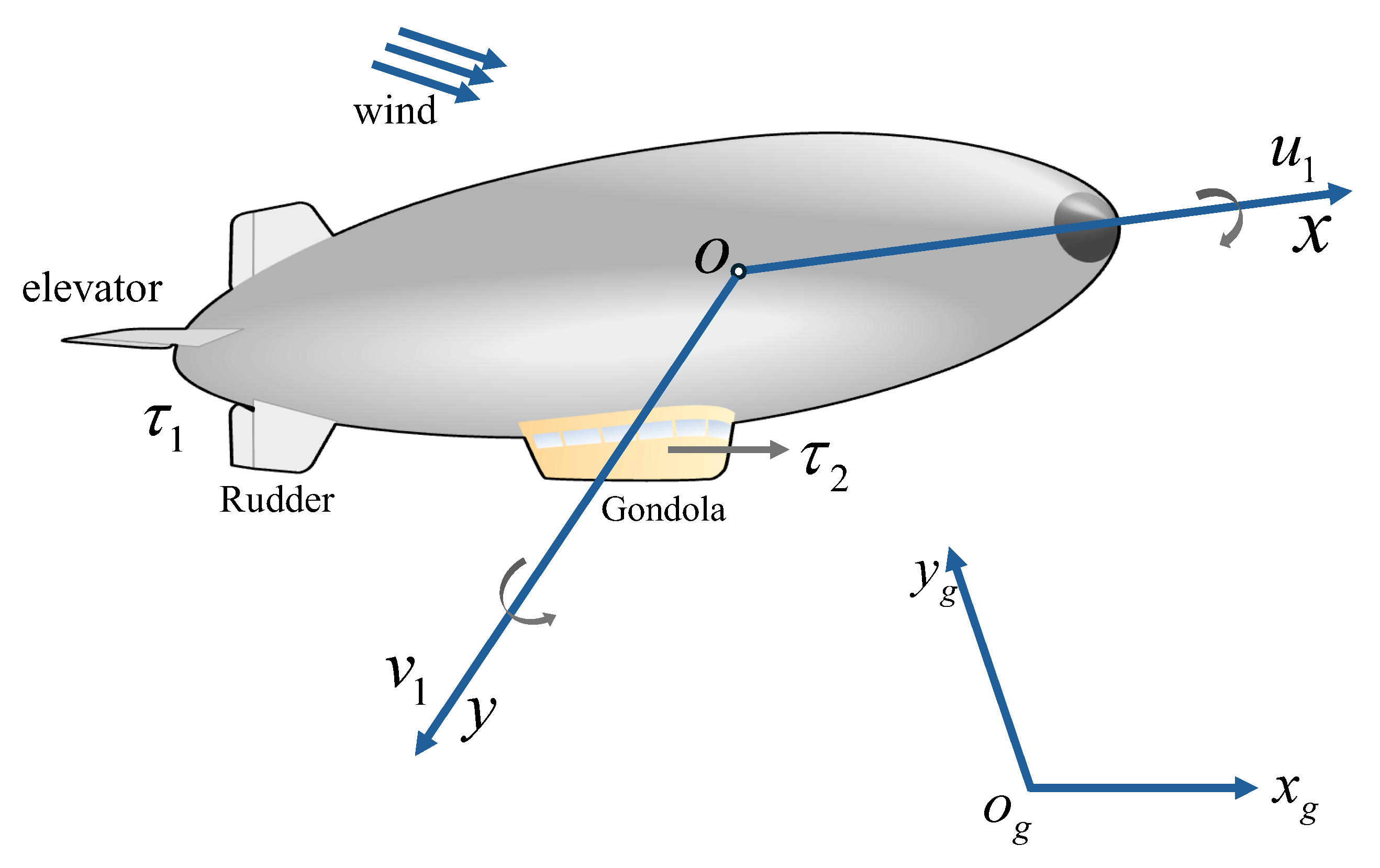
Figure 2.
Integrated Control Architecture for Adaptive Path-Following.
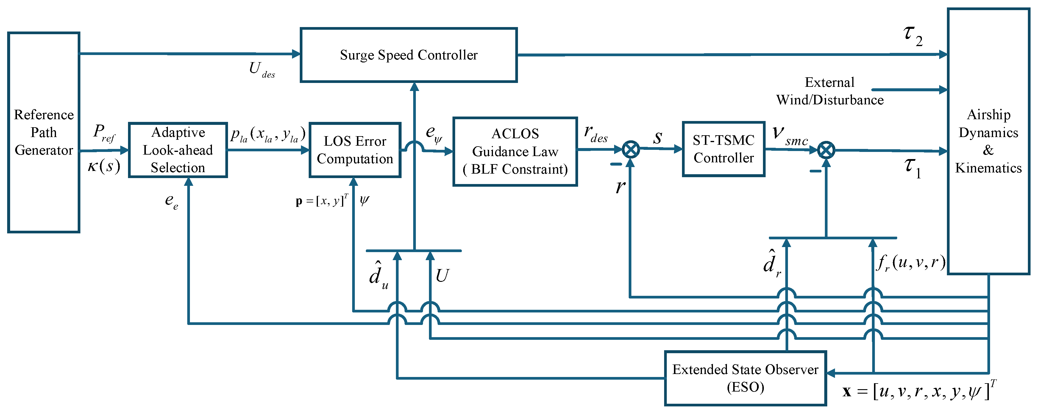
Figure 3.
Comparative planar trajectory tracking under a persistent crosswind disturbance. The proposed ACLOS+ST-TSMC controller (black) is evaluated against conventional ATSMC (blue) and ADRC (cyan) while following a racetrack reference path (dashed red). The enlarged inset highlights tracking behavior in a high-curvature segment, where the proposed method maintains the closest adherence to the reference. The airship’s initial pose is marked by the grey vehicle icon.

Figure 4.
Error Convergence and BLF Constraint Satisfaction. Upper plot: Yaw angle error (solid blue) tracking within its time-varying prescribed constraints (dashed red). Lower plot: Lateral error (solid black) remaining strictly within its adaptive constraints (dashed red).
Figure 4.
Error Convergence and BLF Constraint Satisfaction. Upper plot: Yaw angle error (solid blue) tracking within its time-varying prescribed constraints (dashed red). Lower plot: Lateral error (solid black) remaining strictly within its adaptive constraints (dashed red).
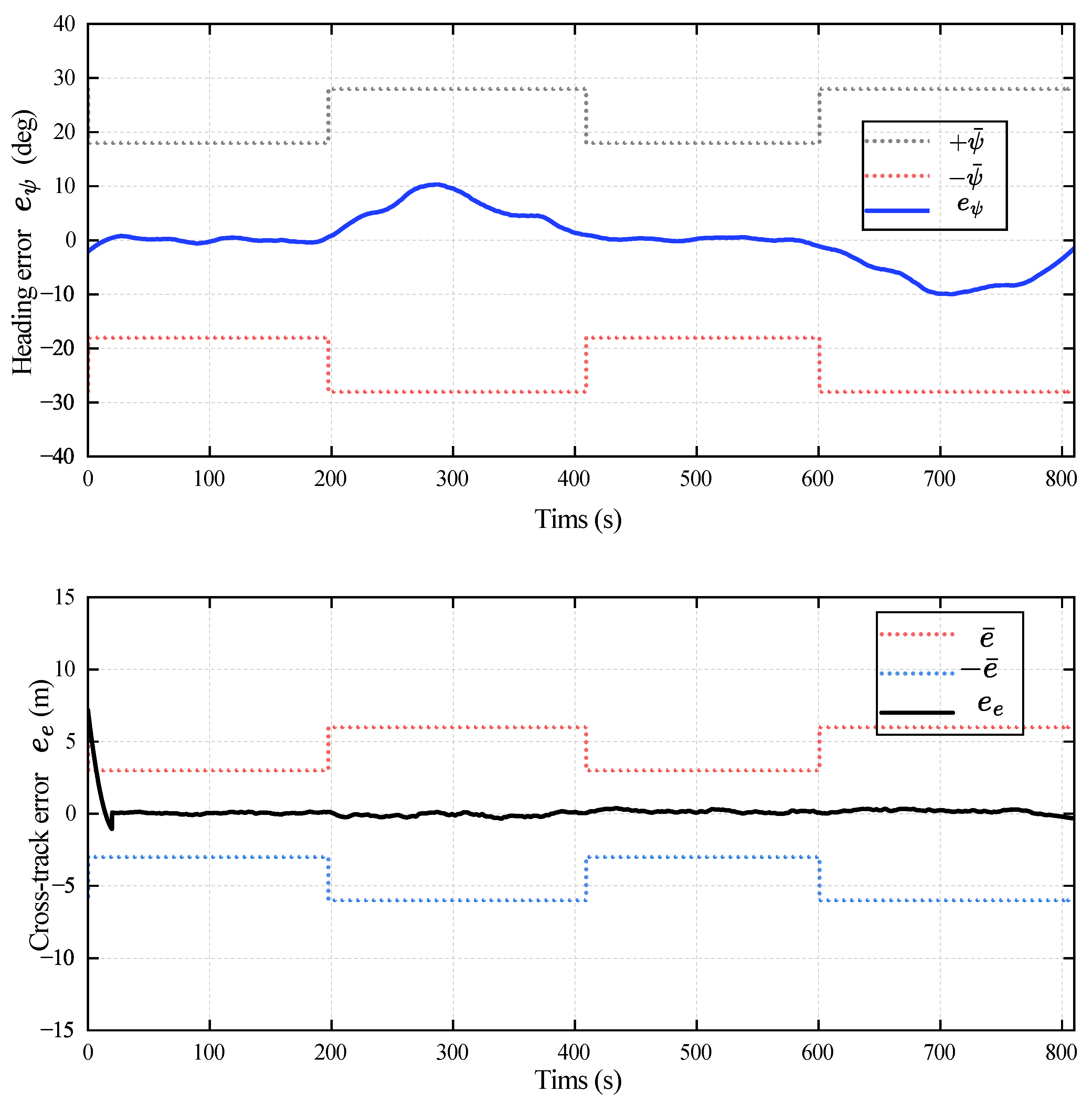
Figure 5.
Real-time Disturbance Estimation via ESO. Validation of the ESO performance for both control channels. Upper plot: Estimation of the lumped yaw disturbance. The ESO estimate (solid red line) is shown to rapidly converge to and accurately track the true disturbance (solid blue line). Lower plot: Estimation of the lumped surge disturbance. The ESO estimate (solid red line) similarly demonstrates fast and precise tracking of the true disturbance (solid blue line). The plots confirm the observer’s rapid convergence (), validating its ability to provide accurate real-time estimates for disturbance feedforward compensation.
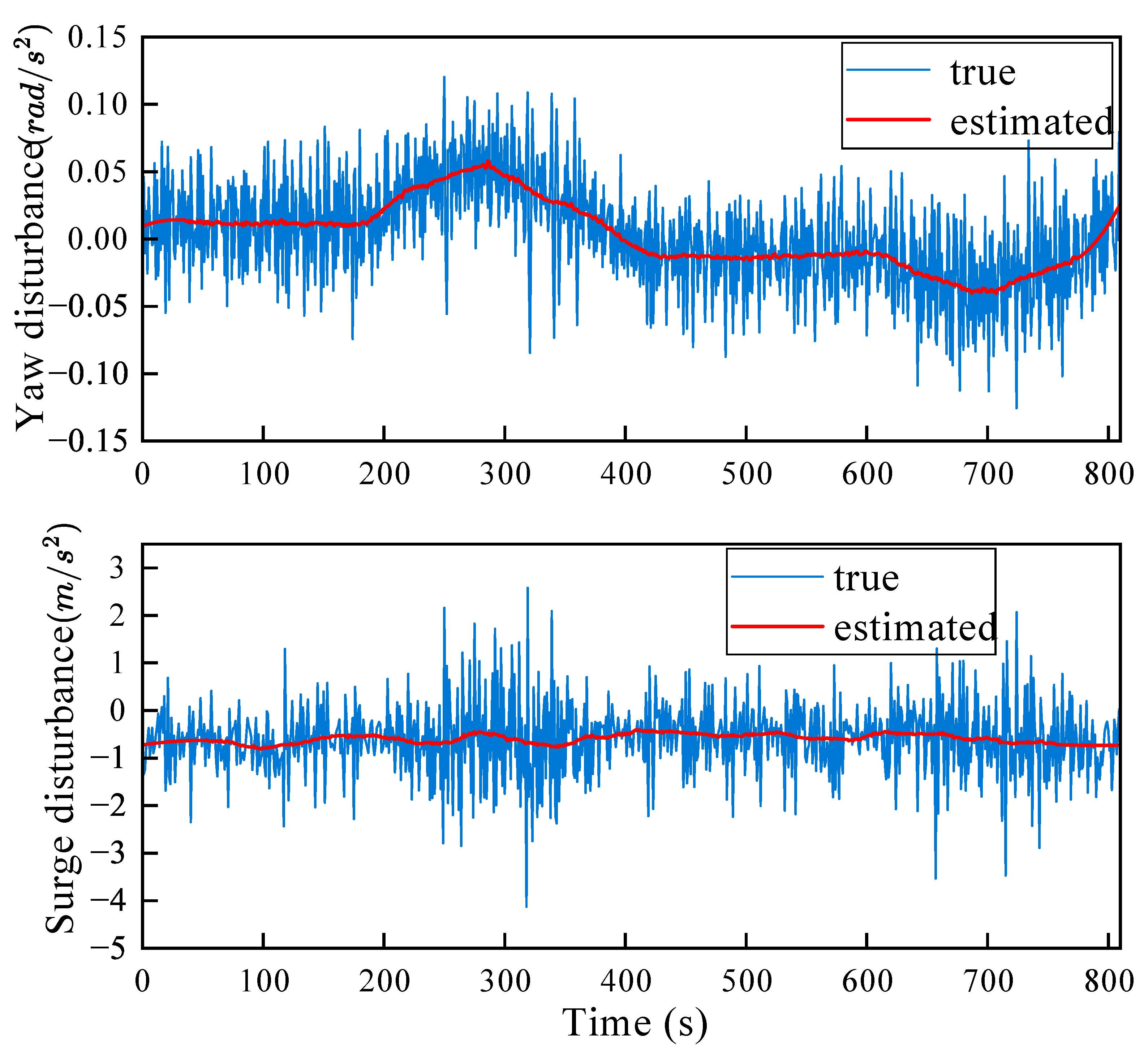
Figure 6.
Analysis of Control Signals and Chattering Suppression. Time histories of the actuator commands. Upper plot: The yaw control torque . Note the smooth, continuous variation, particularly during the high-curvature turn (–300 s). Lower plot: The surge thrust command , which remains stable and smooth. Both signals are continuous and free of high-frequency chattering, confirming that the Super-Twisting SMC (ST-SMC) framework (Eq. 40) successfully generates actuator-friendly commands suitable for practical implementation.
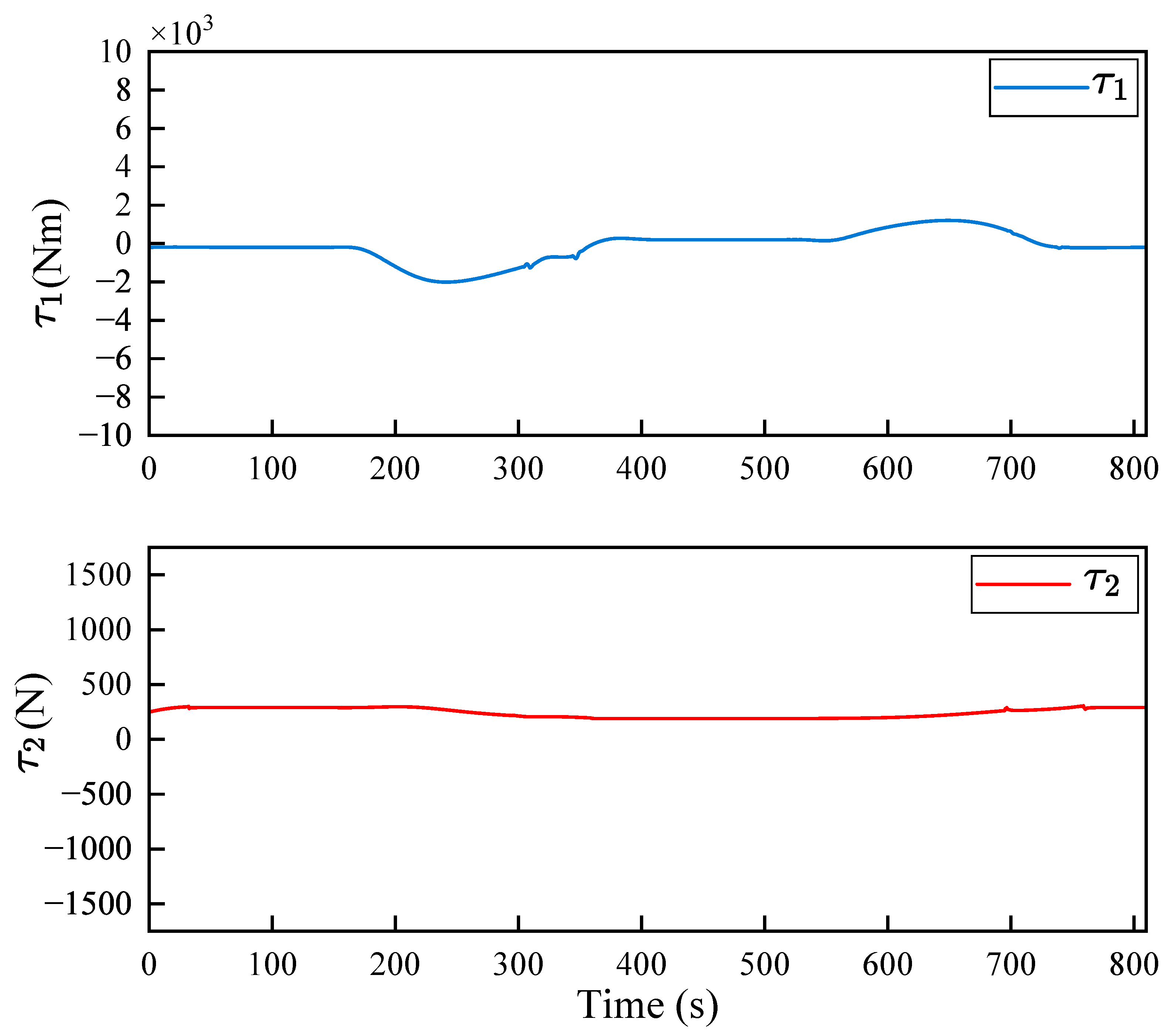
Figure 7.
Robstness to Parametric Uncertainty. Tracking error response under combined mass/inertia and damping perturbations. The plot is a dual-Y-axis time history, showing the lateral error (black, left axis) and LOS heading error (red, right axis) converging while remaining strictly within their adaptive state constraints (dashed blue).
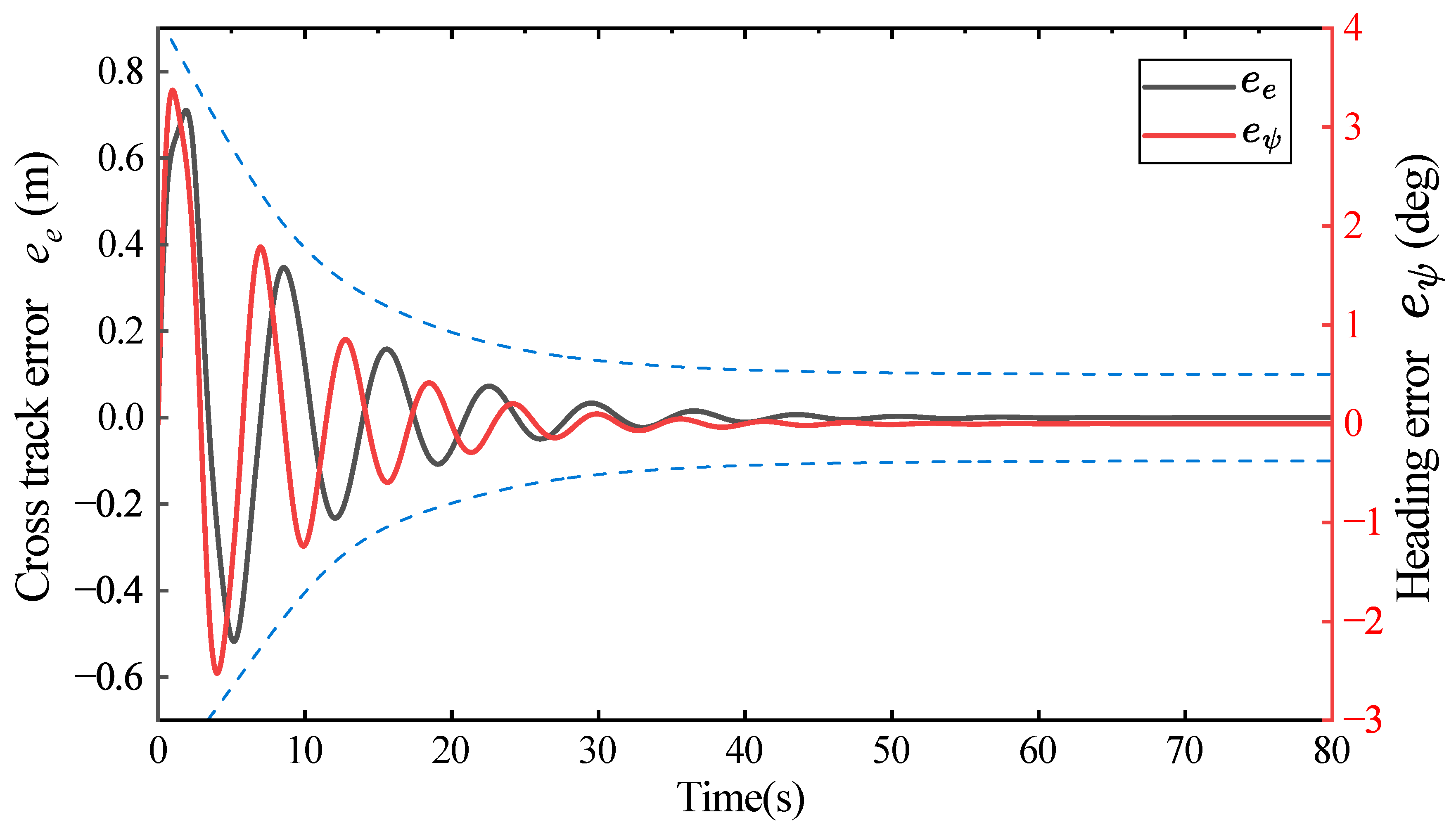
Figure 8.
Validation of disturbance rejection (ESO) and progressive constraint activation (BLF). (a) The injected wind/noise disturbance signal. (b) The ESO’s rapid estimation (red) accurately tracking the true disturbance torque (blue). (c) The BLF value, showing the smooth, stable response of progressive activation (red) versus the chattering of abrupt activation (black). (d) The resulting cross-track error, highlighting the stability of the regulated error (red) versus the raw error’s oscillation (blue).
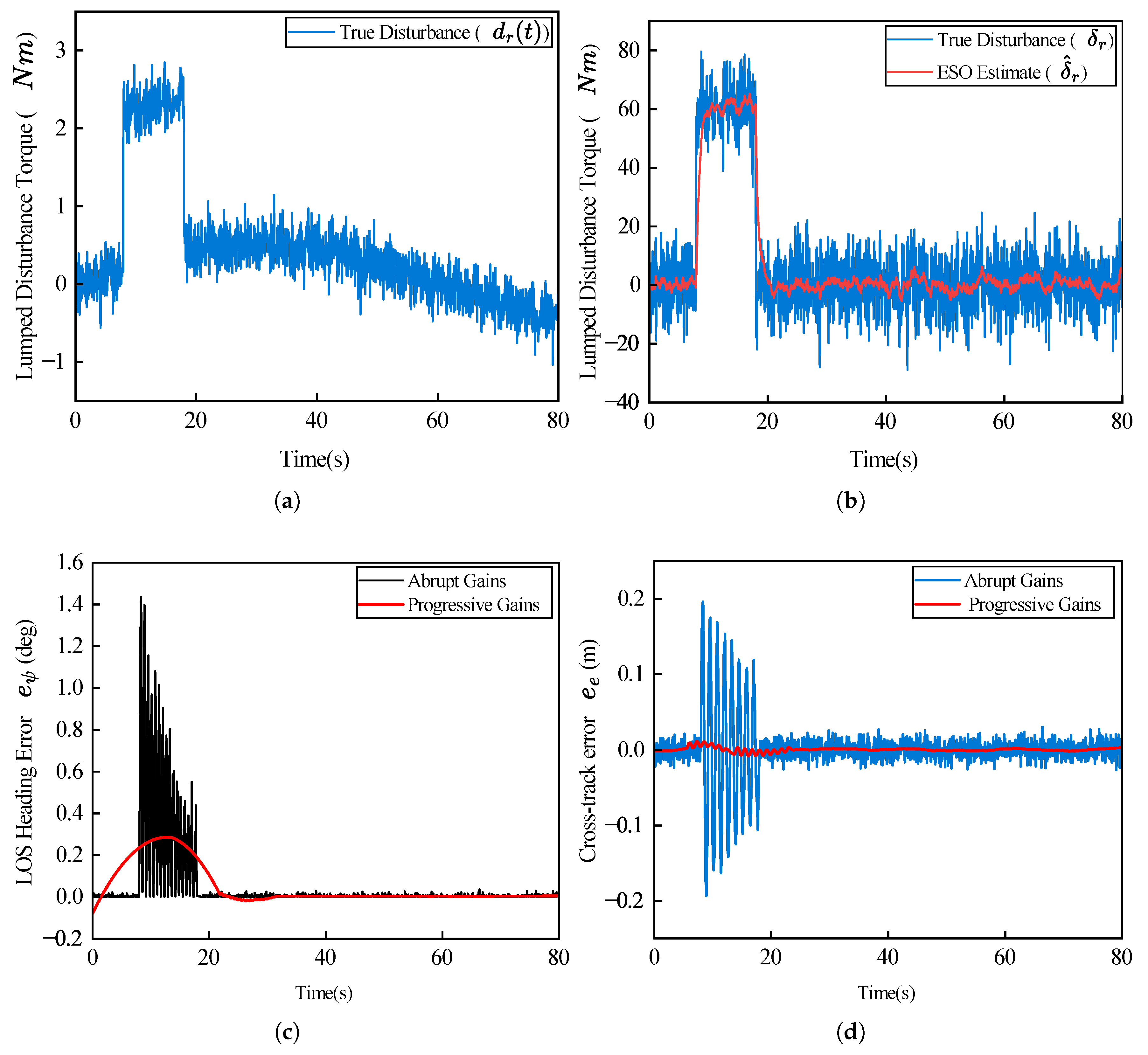

Table 1.
Physical characteristics and uncertainty parameters of the unmanned airship
| Parameter | Description | Value | Unit |
|---|---|---|---|
| Base Parameters | |||
| Yaw Inertia | 12167 | kg | |
| Surge Mass (Inertia) | 301 | kg | |
| Sway Mass (Inertia) | 455 | kg | |
| Yaw Damping | 73 | kg/s | |
| Surge Damping | 50 | kg/s | |
| Sway Damping | 50 | kg/s | |
| Uncertainty Parameters | |||
| Yaw Inertia Uncertainty | 4127 | kg | |
| Surge Mass Uncertainty | 101 | kg | |
| Sway Mass Uncertainty | 155 | kg | |
| Yaw Damping Uncertainty | 13 | kg/s | |
| Surge Damping Uncertainty | 10 | kg/s | |
| Sway Damping Uncertainty | 10 | kg/s | |
| Unmodeled Dynamics | 15 | – | |
Table 2.
Comparative Metrics for Nominal and Perturbed Scenarios.
| Scenario | [ m ] | [°] | |
|---|---|---|---|
| Nominal case | 1.57 | 3.94 | 1.00 |
| +30% mass, -25% damping | 1.76 | 4.25 | 1.07 |
| Relative wind 3 m/s + gust noise | 1.83 | 4.39 | 1.10 |
Table 3.
Quantitative performance comparison among different control strategies.
| Controller | RMS() [m] | RMS() [°] | max() [N·m] | max() [N] |
|---|---|---|---|---|
| Conventional ATSMC | 3.86 | 9.45 | ||
| ESO–SMC | 2.41 | 6.27 | ||
| Proposed ACLOS+ST-TSMC | 1.57 | 3.94 |
Disclaimer/Publisher’s Note: The statements, opinions and data contained in all publications are solely those of the individual author(s) and contributor(s) and not of MDPI and/or the editor(s). MDPI and/or the editor(s) disclaim responsibility for any injury to people or property resulting from any ideas, methods, instructions or products referred to in the content. |
© 2025 by the authors. Licensee MDPI, Basel, Switzerland. This article is an open access article distributed under the terms and conditions of the Creative Commons Attribution (CC BY) license (http://creativecommons.org/licenses/by/4.0/).
Copyright: This open access article is published under a Creative Commons CC BY 4.0 license, which permit the free download, distribution, and reuse, provided that the author and preprint are cited in any reuse.


