

Submitted:
26 August 2025
Posted:
26 August 2025
You are already at the latest version
Abstract
The paper presents a stability analysis of single-channel, slow-rolling, Semi-Automatic Com-mand to Line of Sight (SACLOS) missiles using a comparison of the Routh-Hurwitz and the Frank-Wall stability criteria and a nonlinear analysis. Beginning with a 6-degree-of-freedom (6DOF) model in the Resal frame, a linearized model for the commanded motion is developed. This linearized model, which features complex coefficients due to the coupling of longitudinal channels in rolling missiles, is used to define the structural scheme of the commanded object and its flight quality parameters. The guidance kinematic relations, guidance device equations, and actuator relations, incorporating a switching function specific to slow-rolling single-channel missiles, are also defined and linearized within the Resal frame to construct a comprehensive structural diagram of the SACLOS missile. From this, the characteristic polynomial with com-plex coefficients is derived and analyzed by comparing the Routh-Hurwitz and the Frank-Wall stability criteria. This analysis determines a stability domain for the guidance gain and estab-lishes a minimum limit for the guidance time. The stability domain defined through the linear model is then validated using a nonlinear model in the body frame.
Keywords:
SACLOS missile
; slow‐rolling missile
; single channel command missile
; characteristic polynomial with complex coefficients
; stability criterion
; mathematical model
; Routh‐Hurwitz stability criterion
; Frank‐Wall stability criterion
; flight dynamics
; guidance and control
; Resal frame
; thrust vector control
1. Introduction
In modern anti-armor warfare, guided missiles are a primary tool, often employing "three-point guidance" methods that rely on the alignment of the carrier, missile, and target. These systems can be categorized by their guidance mechanism, with wire-guided missiles typically using angular error control, while laser or radio-beam-guided missiles utilize linear error control. This paper focuses on the former, specifically on wire-guided missiles that require a direct hit on heavily armored targets. This is achieved through a Semi-Automatic Command to Line of Sight (SACLOS) guidance method, where an operator tracks the target, and a guidance signal is automatically generated and transmitted to the missile via a wire.
For subsonic flight regimes, where aerodynamic control surfaces have limited effectiveness, these missiles often rely on gasodynamic controls, such as thrust vector control, to perform necessary maneuvers. The use of slow-rolling missiles in engaging heavily armored targets has become increasingly prevalent in modern weaponry. This design offers several advantages, including a reduction in the missile's size and mass. The rolling motion also serves to cancel out disturbing forces and torques that arise from aerodynamic or gasodynamic asymmetries. Furthermore, the roll allows for control to be executed on a single channel with a single pair of mobile nozzles, simplifying the control system and reducing energy requirements, which is conducive to the development of portable missile systems.
Although these systems are known and technically developed [1,2,3], they represent a special aircraft class, for which, due to the specifics of the movement, theoretical models necessary to clarify some aspects regarding the improvement of their functionality are still in development.
The guidance and control of rolling missiles have been extensively studied. Research has addressed two-channel rolling missiles [4,5], including dual-spin projectiles with high-velocity rotating bodies for gyroscopic stability and lower-velocity rotating tips with canards for trajectory control [6]. Other studies have focused on single-channel missiles with time-modulated commands [7,8,9,10,11]. Recent work on two-channel missiles has explored autopilot design with double [12] or triple [13] feedback loops, the stability of precession motion (conical) [4,5], and the influence of signal errors from the target tracking system [12,14]. Another area of research has been the development of sensors to determine the missile's attitude, particularly the roll angle, which is crucial for command signal generation [15,16]. For instance, some have proposed a new combination of silicon micro-gyroscopes to demodulate yaw, pitch, and spin angular velocities. Another strategy suggested in the literature is the application of a two-step adaptive augmented unscented Kalman filter (TS-AAUKF) [16], which serves to calibrate the magnetometer for accurate roll angle estimation.
To address what was done in the specific case of the single-channel missile, the following section analyses the results from previous research [7–11, 17] in detail.
Reference [7] proposes a digital controller as an alternative to the conventional analogue time-modulation controller. The authors demonstrate that by substituting the analogue phase control with a digital amplitude control system, it is possible to achieve decoupling of the yaw and pitch channels. This method effectively mitigates errors arising from actuator delay and sensor noise. However, the primary limitation of this solution (at the time of proposal) was the increased complexity of the missile's control system, which consequently led to a higher overall cost.
The stability of a rolling rocket with single-channel control is examined in [8] through the development of closed-form analytical solutions from linearized dynamics. This analysis uses a mixed reference frame: the control command is processed in the body frame, while the system dynamics is modelled in the non-rolling Resal frame. Furthermore, the command signal is generated via a series expansion, facilitating a comparative analysis between an idealised rectangular command and a practical implementation that accounts for actuator delays.
In reference [9], a linear model for the commanded motion of a slow-rotating rocket is developed from the equations of motion in the Resal frame. This model uses complex coefficients to account for the coupling between channels caused by gyroscopic and Magnus terms, which allows for the characterization of both nutation and precession motion and the definition of flight quality parameters. This linear analysis concludes in a structural scheme of the commanded object that is specific to slow-rolling missiles with complex coefficients. Unlike the serial development approach in [8], the proposed solution in [9] generates the switch command by considering the sign of a trigonometric expression that depends on the roll angle, as detailed in [18]. The paper analyses two types of single-channel, slow-rolling guided missiles: a portable anti-aircraft homing missile and a portable anti-tank wire-guided missile. In contrast to [8], which formulates the command in the body frame, [9] derives an equivalent command in the Resal frame from the time-modulated command. This equivalent command is then used to construct structural diagrams for both the homing and wire-guided missile types. Due to the complexity introduced by the structural schemes' complex coefficients, the scope was limited to determining the characteristic polynomial's roots and the phase-frequency/amplitude-frequency diagrams for the wire-guided rocket, emphasizing the differences from a non-rolling rocket.
The feasibility of controlling an autonomous rolling rocket via a single-channel reactive command is explored in [10]. The work contrasts a simplified two-nozzle Reaction Control System (RCS) with a conventional six-nozzle configuration. While the traditional system ensures complete three-axis attitude control, the proposed two-nozzle alternative provides actuation for only the pitch and yaw channels. This latter approach leaves the roll angle uncontrolled, thus allowing for free roll rotation of the vehicle.
In [11], starting from the results in paper [9], the case of the anti-aircraft rolling homing missile was analysed, performing a stability analysis with the Frank-Wall criterion.
Reference [17] addresses the optimal control problem for the minimum-time attitude manoeuvring of a rolling missile. In this formulation, a single reaction jet is used to generate the necessary transverse control moments. The problem considers a rocket with an arbitrary initial transverse angular velocity. The objective is to steer the missile to a specified final attitude in the shortest possible time, while simultaneously nullifying the final transverse angular velocity.
The current paper builds upon previous work on single-channel missiles, particularly the findings in [9], by analyzing the stability of a single-channel, slow-rolling SACLOS missile using the Frank-Wall stability criterion [19]. A key distinction between two-channel and single-channel missiles lies in the command formation. While two-channel systems use proportional deflection of both canards, single-channel missiles employ a time-modulated maximum deflection of one canard, managed by a switching function. We will also consider the influence of the guidance gain () and time guidance () of the guided device system, leading to a fifth-order characteristic polynomial, which introduces additional stability conditions that will be analyzed in detail. The effect of phase shift, introduced by actuator delay and inaccuracies in roll angle determination, will also be examined.
Since this paper represents an alternative development of the paper [11], for the case of single-channel slow-rolling missiles with thrust vector control and SACLOS guidance, we will present only the specific elements that appear in this new case, for the common aspects referring to the paper [11].
Contributions of This Paper
This paper presents several key contributions to the study of single-channel, slow-rolling missiles. The primary novelty lies in the comprehensive stability analysis of a SACLOS missile using the comparative Routh-Hurwitz (R-H) and Frank-Wall (F-W) stability criteria and nonlinear analysis. This analysis examines the influence of key guidance system parameters, leading to the definition of specific restrictions and stability domains. To support this analysis, the paper establishes a method for determining the F-W stability parameters for the resulting 5th-order characteristic polynomial, with detailed calculation procedures provided in Appendix E. A detailed structural scheme for a single-channel, slow-rolling SACLOS missile is also developed and presented. Furthermore, this work includes a thorough analysis of the stability and command derivative magnitudes derived from the linearized model, as well as the flight quality parameters. Finally, the stability domains identified through the linear analysis using the R-H and F-W criteria are validated against a nonlinear 6-DOF model, confirming the accuracy and applicability of the results.
The novelty of the paper consists of:
- Comparative analysis between the exact solution and the approximate solution for the equilibrium flight parameters (Section 2);
- The detailed structural scheme for the SACLOS slow-rolling missile with a single-channel (Figure 12);
- Synthesis of the guidance system using the allocation of poly-zeros according to the methodology “Standard coefficient method” (Section 5.6);
- The analysis of the stability of SACLOS missiles using the Routh-Hurwitz criterion for the simplified case without roll. This analysis follows the influence of the main parameters in the missile's guidance system, and stability domains will be defined (Section 7.1).
- The stability analysis for slowly rolling, single-channel SACLOS missiles, employing the Frank-Wall stability criterion. The investigation examines the influence of key guidance system parameters on stability, utilizing a comprehensive model that incorporates higher-order dynamic terms. Based on this analysis, operational constraints are identified, and stability domains are defined for several of these critical parameters. (Section 7.2).
- The evaluation of the Frank-Wall (F-W) stability parameters for 5th order polynomials (the methodology is detailed in Annex E of the paper).
- The validation of linear analysis with R-H and F-W stability criteria using a nonlinear model (Section 7.3)
2. Basic Movement
Since the general equations of motion in the body frame and the Resal frame were presented in the paper [11], to linearize the equations of motion, we will now analyze the basic motion in the Resal frame, because in this case, unlike in [11], we have gasodynamic control.
We will consider a symmetrical evolution in the vertical plane as basic motion. The lateral movement elements are set to zero: . From Figure 1 we can write the equilibrium equations in the vertical plane:
If we detail the lateral accelerations: ; , the relations become:
If the terms of gasodynamic damping [20] are neglected and it is noted
; the thrust components become:
where, as shown in [9,21], the equivalent gasodynamic deflection to the pitch axis of the Resal frame can be taken for twin-channel missiles approximately equal to the deflection in a control plane, and for single-channel missiles it is obtained by integrating the projection of the deflection from the control plane over a period of rotation along the direction of the pitch axis of the quasi-linked frame.
Note: Since in the body frame the position of application of the gasodynamic command is behind the center of mass, it follows .
The aerodynamic coefficients are developed in this way:
For analyzing the magnitude terms in these expressions, and those that will be elaborated later, we will use, according to [22,23], the following parameters:
Small values:
- reference time;
- reduced gravitational acceleration
Large values:
- the reduced mass of the aircraft
-the reduced moment of inertia in pitch
Introducing these parameters into relations (2), we obtain:
where we noted ; while is the dimensionless angular rate of precession, and is the flight-path inclination angle.
If we impose angular velocities , and the angle of inclination of the trajectory , the system (5) can be solved numerically with a Newton algorithm [24] in relation to the sizes , , , which represent the flight parameters for the basic motion under consideration.
If we impose a translational motion with zero angular velocity of pitch and yaw (, and neglecting the aerodynamic terms of higher order (, the system decouples and becomes:
One can notice that for lateral motion the last two homogeneous equations lead to the trivial solution: ; while the first two equations, corresponding to longitudinal motion, for the given lead to a transcendent equation in the angle and a calculus relation for the equivalent thrust deflection in pitch .
Thus, eliminating the incidence between the equations of longitudinal motion, we obtain:
where the static stability reserve was noted..
If the terms of the thrust are eliminated, the following is obtained:
Imposing the value of the climb angle , implicitly for the particular case of horizontal flight , the system is reduced to the relation (8) which becomes a transcendent equation that is solved iteratively in relation to the incidence to which is added the explicit relation (7) which allows the determination of the equivalent thrust angular deflection.
Figure 2.
Comparison between the exact solution (5) and the approximate solution (7) (8) for the equilibrium command - initial mass values.
Figure 2.
Comparison between the exact solution (5) and the approximate solution (7) (8) for the equilibrium command - initial mass values.
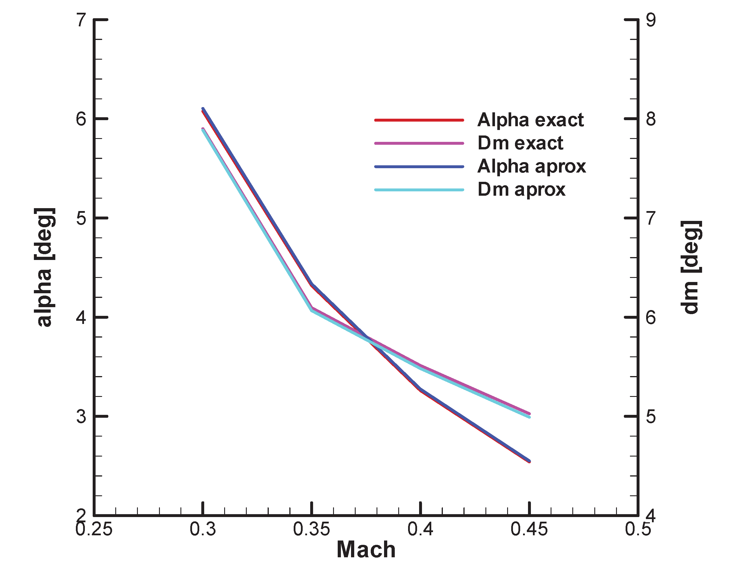
Figure 3.
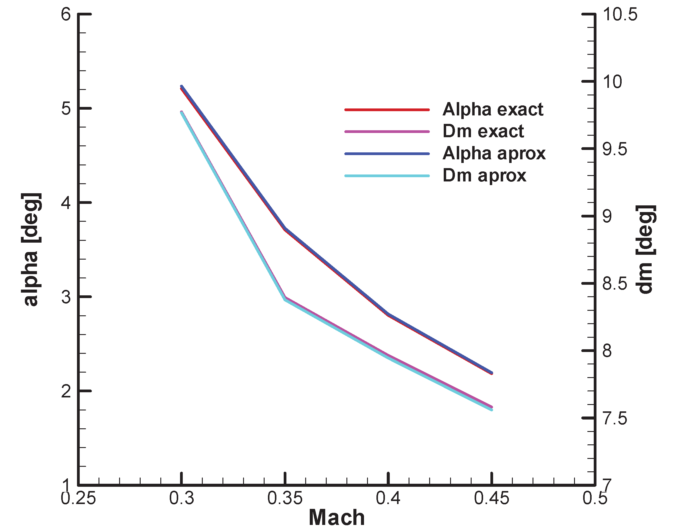
Comparison between the exact solution (5) and the approximate solution (7) (8) for the equilibrium command - final mass values.
Figure 3.
Comparison between the exact solution (5) and the approximate solution (7) (8) for the equilibrium command - final mass values.
These parameters (represent the basic movement of the rolling missile, presented in Appendix B.
From Figure 4 it can be seen that the equilibrium incidence in the lateral plane (β) is negative, which will lead to a deviation of the trajectory to the left of the firing plane, a phenomenon specific to aerodynamically stabilized rolling missiles.
3. The Linear Equations
To obtain the linear equations, we will consider the hypotheses from the work [11].
Also, for the symmetry, for the gasodynamic commands, we will consider the small angular deflections so that:
Linearizing translational equations in the Resal frame [11], we obtain:
On the other hand, linearizing rotational equations in the Resal frame [11], we obtain:
For coupling the equations, similar to the paper [11], the following dual notations are made:
These parameters represent the stability and command derivatives that are presented in Appendix B.
Next, we will rewrite the coefficients of the equations of motion, in which we will include the previously defined parameters for the basic movement, obtaining:
Also, we define the complex quantities:
with: .
In this case the equations (10) and (11) are:
Applying the Laplace transform, the homogeneous form is:
with the characteristic polynomial:
Separating complex terms, we will obtain:
With the approximations (13), the characteristic polynomial becomes:
where will be explained later.
To verify the correctness of relations (13), in Figure 5 and Figure 6 the roots of the characteristic polynomial obtained with the approximate relation (19) and the exact relation (18) are presented comparatively. The diagrams are obtained for a range of Mach numbers: 0.3...0.45.
Based on these results, the approximate relations (13) will be used to obtain the simplified structural scheme for the commanded object.
4. The Flight Quality Parameters
For the considered configuration, similar to the work [11], the following notations are defined:
where is the angular rate of precession, with dimensionless form and represents static stability (Figure B17).
In this case, the characteristic polynomial (19) has the form:
with natural pulsation and damping factor having the expressions:
Sometimes, the inverse of natural pulsation is used:
- time constant of nutation movement.
In Figure B18, Figure B19 and Figure B21 from Appendix B the natural pulsation, damping factor and time constant according to the Mach number are presented.
The roots of the characteristic polynomial (21) are:
Developing we obtain:
where: ; ; To obtain the command parameter, we put the relation (15) in matrix form:
with the inverse matrix:
where is the characteristic polynomial.
Based on this relation, as shown in [11], after processing, the following transfer function is obtained:
where the input is the complex form of gasodynamic deflection in the Resal frame and the output represents the complex form of the angular velocity of the velocity vector.
With the notations:
the transfer function, due to the large value of the parameter , becomes:
where the following notations were made:
the command factor and the parameter
the advance time on command or the aircraft's time constant [25]
and is a Magnus term.
Dropping the secondary terms for the gasodynamic commanded missile, the parameters from the relations (28) become:
where we recall that it was noted: where represents the distance between the point of application of the gasodynamic control and the center of mass, in the body frame, having a negative value.
We can also evaluate the complex acceleration in the Resal frame:
with:
Based on these relations, we can build the structural scheme of the commanded movement for slow-rolling missiles, with gasodynamic command, shown in Figure 7.
5. The Guided Flight Model
5.1. The Guidance Relations
As shown in [21,26,27], the guidance kinematic relations will be constructed into a frame linked to the carrier - target line of sight called the guiding frame (Figure 8). The guiding frame originates at point (, which represents the position of the carrier, the axis pointed target , the axis is in a vertical plane facing downwards, and the axis horizontally, it follows from the condition of the right frame. The guiding frame is non-inertial.
In the case of angular deviation control, the guidance parameters are: , for determining which relations are used:
and:
From Figure 9 and Figure 10 it is observed that the angular error in the two guidance planes can be expressed as follows:
Assuming that the target, the carrier and the mobile evolve independently in the two planes, the geometric connection between the angles can be derived, obtaining:
where the angular velocities were noted:
5.2. Linear Form of Kinematic Guidance Relations
In the case of semiautomatic command to line of sight (SACLOS), which is based on angular error control, the collinearity of the three points (A-M-T) is achieved by cancelling the angular deviation in the two guidance planes:
Considering the geometric connections between angles in the guiding planes (35), one can write:
which represents the collinearity of the position vectors for target and missile Figure 8.
If the condition of cancelling the rate of the deviations is also imposed:
relation (36) show:
which is the condition that the vectors and rotate with the same angular velocity.
To construct a model of guidance with angular deviation control, we start from the observation that the linear shape of the guide controls is decoupled for the case of a general movement.
Thus, if the definition relation of the angular errors is linearized:
under the conditions of the basic movement, the following is obtained:
By entering the expression of the linear deviation previously established, we obtain:
On the other hand:
In this case, the deviation of the angular errors becomes:
From whence:
Considering the particularity of the basic movement adopted, in which the velocity vector of the mobile is collinear with the target's line of sight, namely:
and noting the input functions of order "0" due to the carrier's position deviations:
the deviation of the angular error can be put in the form:
thus, obtaining the cinematic block.
From this relation it can be seen that for the case of the fixed carrier the deviation of the absolute angle of the line of sight of the missile is given by:
On the other hand, the guidance commands in the guidance planes are:
where:
By applying the Laplace transform, the guidance command can be put in the form:
For the linearization of the guidance command, a particular basic motion is considered, where the target, the mobile and the carrier are collinear and the velocity vector of the missile is oriented along this line.
In this case, the angle of lateral inclination of the missile must be zero, the head angle of the missile is equal to the angle of rotation in the horizontal plane of the guidance frame , which overlaps the pitch plane of the missile with the vertical plane of guidance.
The axis of the rocket is above the velocity vector, with which it forms a positive incidence that balances the force of weight.
For the simplification of the structural scheme, in the case of the fixed carrier, the zero-order input functions can be considered cumulated with the inputs due to the target through the angles , obtaining in this case a simplified transfer function, with a single input.
5.3. The Guidance Command
As shown in the paper [11], neglecting the angle of incidence in the vertical plane, and assuming that the pitch angle of the rocket overlaps angle of the guiding frame, the command can be put in the following form:
where the following notation was made:
being the direct rotation matrix with roll angle.
Next, we will seek to bring matrix expressions to complex form using a polar coordinate system that highlights the module and phase of the guidance command. Thus, if the commands are put in the complex form:
where is the command in body frame and is the command in the guiding frame / Resal frame.
In this case, the relation (55) becomes:
Base on Figure 11, the guidance command can be put in polar coordinates:
where:
– is the command module; – is the command phase.
In this case, the command for the two channels (pitch and yaw) in the body frame becomes:
where is the phase shift, the significance of this angular error being detailed in work [11].
As we showed in papers [9] and [11], for the single-channel case we can give up one component of the command in the body frame, obtaining in the guiding frame a command oriented in both directions due to the roll rotation.
To obtain the time modulation of the command for a single-channel missile, it is necessary to use a switching function of the form indicated in work [18]:
where , called the fill factor, is given by the relation:
in which is the command module, is the maximum guidance command, and the argument , called the relative roll angle, is given by:
where represents the command phase (Figure 11), is the roll angle and is the phase shift.
The switching function (61) is applied instantaneously through a nonlinear element, relay-type, the pitch canard deflection angle being:
As shown in the [18] for the expression of the equivalent command, the weight compensation command is also entered. This is achieved by the equilibrium fill factor for a horizontal base motion, which is a function of the ratio of the weight compensation control component to the maximum order value:
Unlike the roll-stabilized missile, where the balance command can be achieved directly by changing the zero position of the command surfaces (canard, elevator), in the case of rolling missiles, the equivalent balance command is introduced by the guidance term; in this case, the balance control is non-zero. Resuming the linear relation established in the works [11] and [9] can be written as:
which expresses the connection in deviations between the command and the thrust equivalent deflection.
Similarly, for the absolute angles of the target's line of sight, the quantity is defined:
and from the angular deviations in the guiding planes, the following are obtained:
where:
Between the three complex quantities defined above there is the relationship:
Finally, it is also possible to define the complex form of the zero-order entry function in the system due exclusively to the operator or the sighting device:
function that will be cumulated with the absolute angle of the target's line of sight ().
Processing of the error signal and formation of the guidance control signal is done using a P.D. (derivative proportional) type element that has the following known structure:
where and are guidance gains, and is a time constant that eliminates high frequencies.
NOTE - In case of Manual Command to Line of Sight (MCLOS), the control is done manually by a human operator, as indicated in the paper [18], and the signal can be shaped by a transfer function:
an expression which, as indicated in the same paper, can be approximated with:
5.4. The Structural Scheme
Next, in order to build the structural scheme of the SACLOS, it is necessary to define the complex shape of some pairs of kinematic parameters in the guiding planes.
Thus, for the absolute angles of the rocket's line of sight, the complex size can be defined:
5.5. Determination of the Characteristic Polynomial
For the analysis of the stability, the transfer function of the open system is first determined:
where we considered null the phase shift introduced by the actuator , and we noted the guidance gain:
and the guidance time:
In this case, the transfer function of the closed system becomes:
where represents one's pulsation.
For the stability check we develop the characteristic polynomial from the denominator of the transfer function.
The characteristic polynomial, after ordering, becomes:
For the stability analysis, we put the polynomial in the form:
where:
5.6. The Guidance System Synthesis
At this point we aim to determine the three parameters of the guidance system:.
To begin with, we will neglect the complex coefficients, considering a regular missile without roll rotation. In this case, the transfer function of the closed system (79) becomes:
Next, we will use an allocation of poly-zeros according to the methodology “Standard coefficient method” from the paper [28]. This analysis can give us indicative information on the main control parameters of the system.
According to the methodology, for the transfer function obtained (84), with a characteristic polynomial of order 5, the recommended transfer function is of the form:
where with the desired system response time.
By identifying the coefficients of the characteristic polynomial of the two transfer functions, the following relations are obtained:
The main quantities that intervene in these relations and that are related to the dynamics of the missile are:
– pulsation; – damping factor and – amplification factor that intervenes in the gain .
The values of these quantities are presented graphically according to the Mach number in the initial phase (with fuel) and in the final phase (without fuel) in Annex B of the work
From the diagrams (Annex B), for the analyzed velocity range , the parameters have the values: ; ; ;
From the last two relations (85) is obtained:
Eliminating , the equation follows:
with the positive solution:
For the range of values of pulsation and damping factor , the solution has the following values: ...3.85
From , the response time can be estimated:
Since the response time of the system must be low enough to combat close targets, we choose , from which it follows .
From the third relation (85) we get:
which for the pulsation values range , has values in the range of:
Combining the second relation (85) with the relation (89) yields:
for which an estimate of the gain is needed.
Considering approximate relations (30) we obtain:
The parameters that intervene in the expression of gain are ; ; ; ; from which it follows: ;
For this range of variation of the gain from (90) we obtain:
Based on the results obtained, the values adopted are:
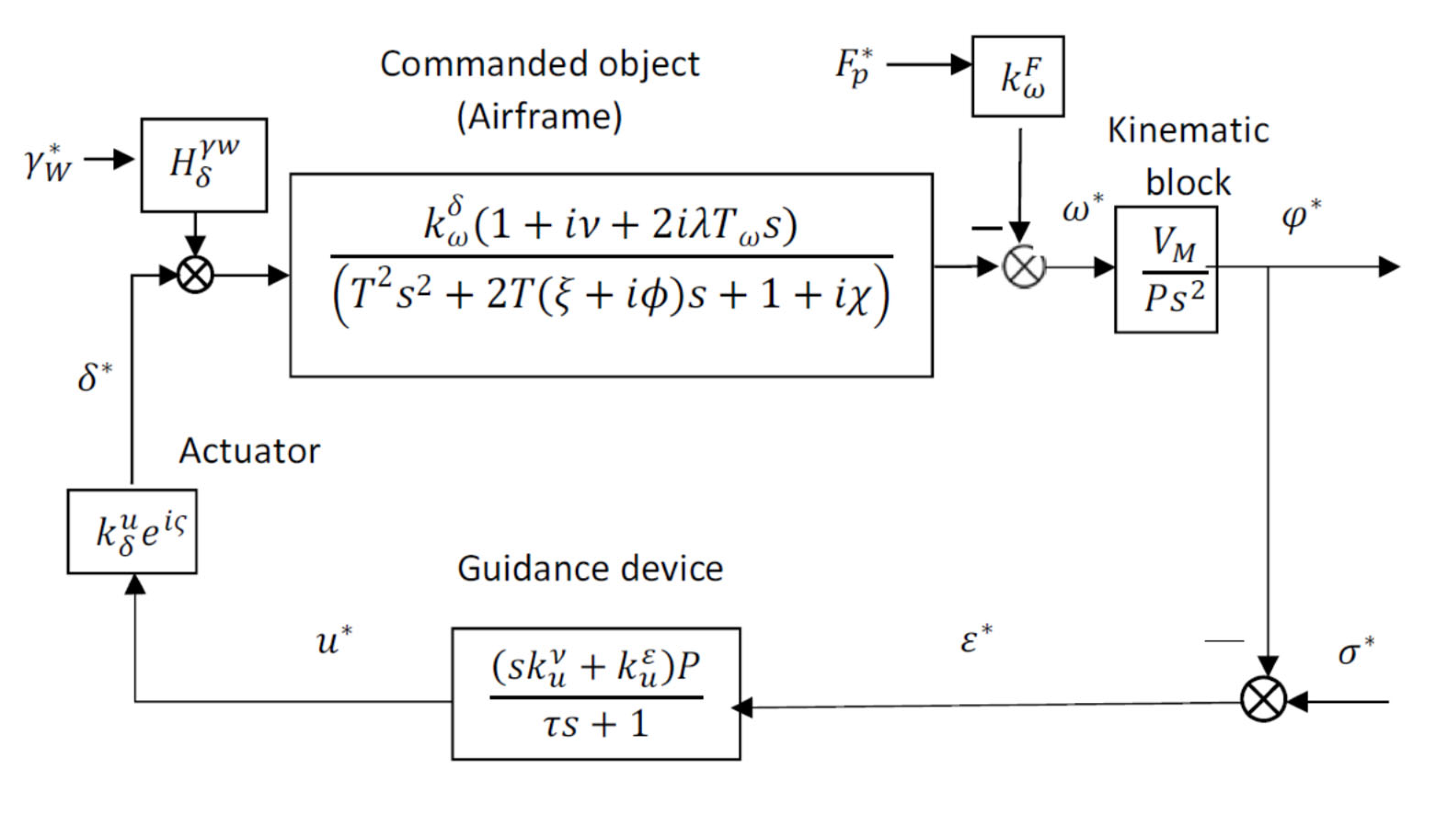
Based on the relations thus obtained, the structural scheme for the SACLOS single-channel rolling missile controlling the angular deviation in the case of the fixed carrier are presented in Figure 12
Figure 12.
Structural scheme for rolling single-channel SACLOS missile.
6. Calculus Model
To obtain numerical results, we will further specify the data of the calculus model.
6.1. Aerodynamic Characteristics
The aerodynamic characteristics were determined using the configuration from Figure 13.
Considering the specifics of the configuration and the flight regimes, starting from the regular aerodynamic coefficients indicated in [29] and [30], according [31] we introduce additional terms that contain influence of rotational and non-stationary motion and combinations with incidences.
Thus, the development of aerodynamic coefficients in the body frame for the slow-rolling airframe from Figure 13 is given by:
where, the rotational velocities and non-stationary translational variables are considered dimensionless, according to the standards [22,31] are:
The terms of development of aerodynamic coefficients are presented against the Mach number in Appendix A.
6.2. Mechanical and Reference Characteristics
The mechanical characteristics of the model are indicated in Table 1

Table 1.
Mechanical characteristics.
| Phase | Mass m[kg] |
Center of Mass [m] | Roll Inertial Moment A [] | Yaw/Pitch Inertial Moment B | Time [s] |
| Start | 11.4 | 0.49 | 0.021 | 0.373 | 0 |
| Initial (1 | 10.6 | 0.50 | 0.018 | 0.364 | 0.65 |
| Final | 8.6 | 0.49 | 0.016 | 0.341 | 27. |
1After finishing the booster.
For the considered configuration, the reference length is reference surface is , and the maximum angular thrust deflection is .
6.3. Thrust Characteristic
The thrust characteristic of the model is shown in Figure 14.
6.4. Time Constants and Controller Gains
As basic data for the linear model, the following parameters were considered:
7. Stability Analysis of the Single-Channel SACLOS Slow-Rolling Missile
7.1. Stability Analysis with the Routh–Hurwitz Criterion
Further, neglecting complex terms, we will do a stability analysis with the Routh-Hurwitz criterion to highlight restrictions on the guidance and control parameters.
The Routh–Hurwitz conditions for the 5th order polynomial with real coefficients are obtained from the matrix of coefficients constructed as follows:
From condition: results successively:
From condition: is obtained successively:
For stabile missile, with and relation (97) is always satisfied, being quadratic equations inwith complex conjugate roots.
From the condition , results successively:
Since is linear in, condition (98) becomes:
relation that allows obtaining the stability domain related to for fixed.
From condition results successively:
Since is quadratic in , the second condition (100) becomes:
The relations (99) and (101) allow obtaining the stability domains related to and .
Figure 15 and Figure 16 show the corresponding stability domains for and , obtained with relations (99) and (101), for fixed at operating point ( in the initial and final of the second phase.
It can be seen from the two diagrams that the stability domain for is more restrictive than that for , and hence only the domain corresponding to will be taken into consideration.
In addition, the domain highlights the inner limit of :
where the gain becomes zero.
Applying relations (99) and (101) over the entire Mach number range, the diagrams from Figure 17 and Figure 18 are obtained. It can be seen from these diagrams that the limit is always more restrictive than and that the current value of the gains falls within the stability domain over the entire Mach number range.
To summarize, for a regular system with a subunitary damping factor (0) and the time constant of the nutation positive , the only constraints that remain active are those given by which limits the guidance gain and lower limits the guidance time and which lower limits the time constant ().
The result obtained is equivalent to the criterion Liénard–Chipart, which for the 5th order polynomial with real coefficients imposes the following conditions [32]:
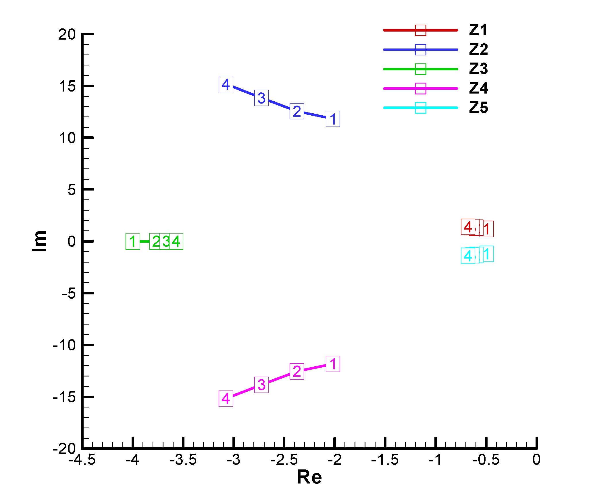
As an additional check, in Figure D1 and Figure D2, the roots of the characteristic polynomial with real coefficients at the operating point, analyzed by the conditions R-H, are presented. It is observed that the polynomial has four conjugate complex roots with negative real parts and a negative real root, which confirms the stability of the analyzed system.
Next, we will analyze the characteristic polynomial of the system, considering the complex part of its terms using the stability criterion Frank-Wall.
7.2. Stability Analysis with the Frank-Wall Criterion
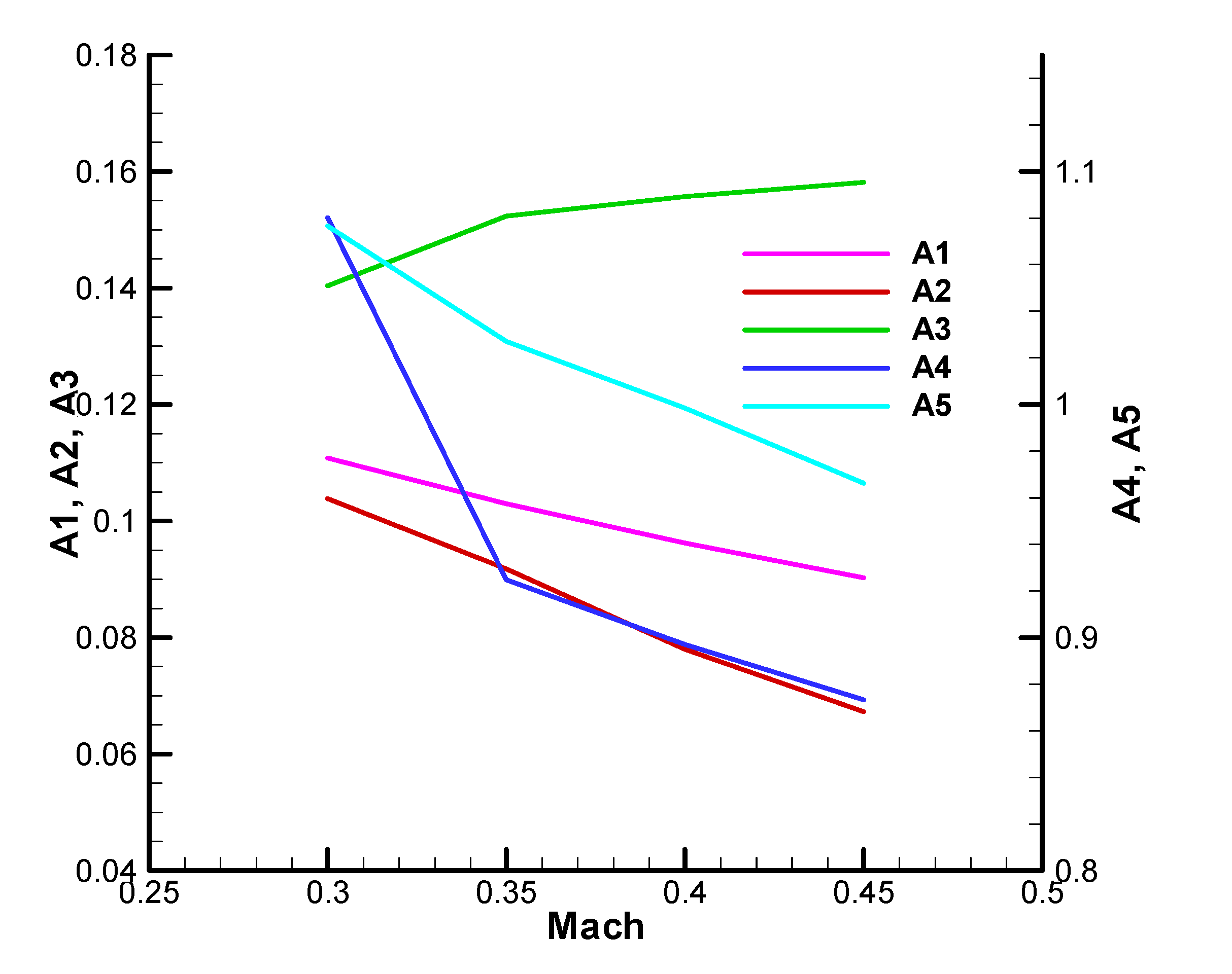
Based on the relations (E 5), (E 6), (E 7) and the characteristic polynomial coefficients, the Frank-Wall parameters ( were determined and graphically shown in Appendix C. For the basic input data considered, the stability criterion F-W is met: , as we can see from Figure C9, Figure C10, Figure C11 and Figure C12. It is observed that they are positive over the entire domain, which means that the roots of the characteristic polynomial will have real negative parts.
Next, we will analyze the root locus of the characteristic polynomial (Appendix D) To begin, we shall consider the basic test case set out in section 7.3, Table 1, for the second phase of flight at two points, at the beginning () and the end of the phase (). The analysis is done on the range of Mach numbers corresponding to phase 2 ( ) at ground level. A first observation of a general nature is that the roots do not have a symmetrical distribution with respect to the real axis, as in the case of stabilized roll rockets, where the characteristic polynomial has real coefficients. There are five roots of the polynomial, thus:
- Roots 2 and 4 are close to those of the characteristic polynomial of the commanded object (23) or (24)(24) which has a negative real part and large complex parts that are almost conjugate.
- Root 3 is large in module, with a negative real part and a small complex part, due to guidance control.
- Roots 1 and 5 are small in module, with negative real parts and small complex parts due to the guidance loop
Figure D3 and Figure D4 present the roots of the characteristic polynomial with complex coefficients for the initial point of the second phase without phase shift ) and with phase shift (.
Figure D5 and Figure D6 present the roots of the characteristic polynomial with complex coefficients for the final point of the second phase, without phase shift () and with a phase shift In this case, unlike the case with real coefficients previously analyzed (Figure D1 and Figure D2 ), we have five complex roots arranged non-symmetrically related to the real axis, that is, we no longer have complex conjugate roots. However, it is observed that the real part of the roots is negative in all cases, which ensures the stability of the analyzed system.
It is of interest to verify whether, in the case of the missile with rolling rotation (polynomial with complex coefficients), we obtain the same stability domains as in the case of the R-H analysis for a missile without rolling (polynomial with real coefficients).
Unfortunately, because the F-W calculation relations are complicated, we cannot find an analytic solution like in the R-H case. Therefore, we will summarize some numerical results for verification.
Thus, in Figure 19, Figure 20, Figure 21 and Figure 22 the variation of the F-W parameters is presented depending on the guidance gain . It is observed that the cancellation of these parameters (), that is, the limit of the stability domain, is done by a jump from the positive to the negative value. The jump is explained by the fact that these points are close to the points of cancellation of the R-H determinants and by the relation (E 8), between the determinants R-H and the parameters F-W, in which the determinant R-H is in the denominator of the parameter F-W. Due to the jump at the point of cancellation, determining an exact solution numerically for these points is difficult.
From the analysis of the diagrams, it is observed that for the condition is similar to is found, i.e. , and for the stability conditions similar to are found, i.e. we have a domain for between and . The condition is also found, i.e. the stability condition for is more restrictive than . As for , this introduces a condition similar to . Regarding and , these parameters were not analyzed because they do not depend on the gain .
It can be seen from the figures that in the initial phase (Figure 19,Figure 20) the cancellation values are smaller and in the final phase (Figure 21, Figure 22), which means that the domain of stability is more restricted in the initial phase. Also, in the initial phase, a third cancellation point is observed, which is not found in the final phase nor in the R-H analysis. Regarding the shift phase, it is observed that this leads to a decrease in the upper cancellation point , therefore there is a slight decrease in the stability domain.
It can be seen from the two diagrams that the stability domain for is more restrictive than that for , and hence only the domain corresponding to will be taken into consideration.
In addition, the domain highlights the inner limit of from relation (102).
The stability domains are presented for the initial moment (Mach=0.3) and the final moment (Mach=0.45). Similar to the R-H analysis, it is observed that in the case of the F-W analysis, the stability domain is smaller in the initial phase than in the final phase of the guided flight.
Figure 23.
Stability F-W domains Mach=0.3;- initial.
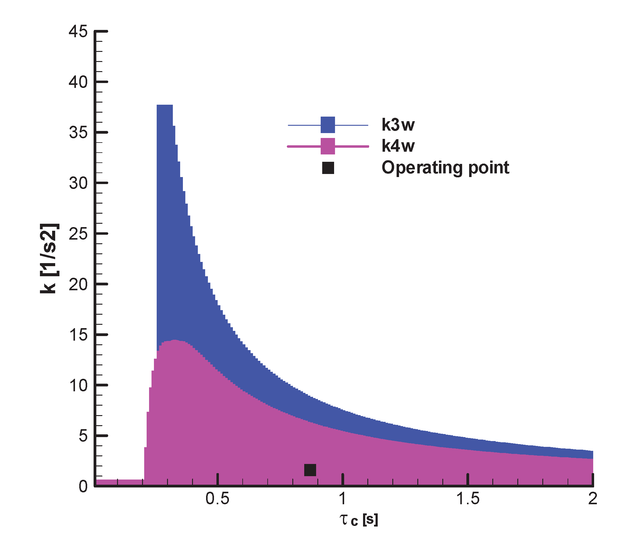
Figure 24.
Stability F-W domains Mach=0.45, ; – final.
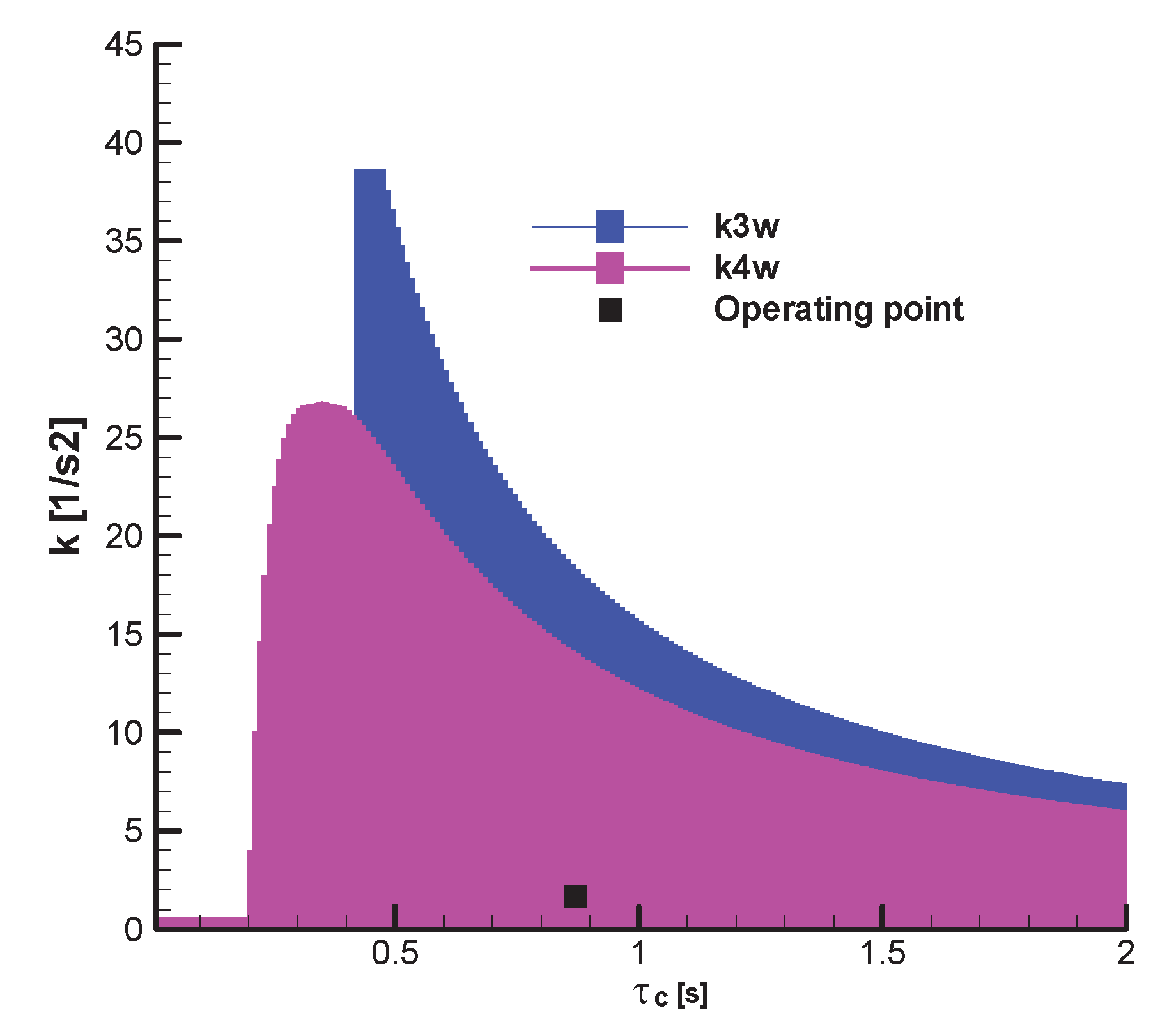
From the previous analysis it follows that the most restrictive stability domain F-W, which must be considered, depends on the first point of cancellation of , namely To have a comparative picture, in Figure 25 and Figure 26, the stability range obtained with the R-H criterion and the stability range obtained with the F-W criterion are presented together.
Thus, in Figure 25 and Figure 26 the stability range of the gain as a function of the guiding time for a fixed time constant. It is also observed from all the diagrams, that for the considered operating range, the F-W stability domain is reduced compared to the R-H domain, which represents an important result in the comparative analysis performed.
To exemplify the result of the previous analysis, we will start from the operating point and increase the gain until we obtain instability on the F-W criterion. Then we will check whether stability is maintained for the R-H criterion at that new operating point.
Thus, if we increase from to , and the other parameters remain unchanged (, ), the F-W parameter that will become negative will be , as can be seen from Figure 27.
At the same time, one root of the characteristic polynomial with complex coefficients has a positive real part, as seen in Figure 28. The diagram is obtained for a range of Mach numbers 0.3...0.45.
On the other hand, from Figure 29 it can be seen that for the gain k value is maintained in the stability range (R-H) determined on the polynomial with real coefficients but is out of the stability range (F-W) determined on the polynomial with complex coefficients.
Moreover, for this case, the roots of the characteristic polynomial with real coefficients have a negative real part, as can be seen from Figure 30. The diagram is obtained for a range of Mach numbers: 0.3...0.45.
This means that for the case of a rolling missile, the stability analysis on the polynomial with real coefficients, in this case R-H, is not sufficient, requiring an additional analysis on the polynomial with complex coefficients of the F-W type and an evaluation on the nonlinear model, as we will proceed further.
7.3. Stability Analysis Based on the Nonlinear Model
Based on equations of motion in the body frame [11], and kinematic guidance relations (33), (34), as well as guidance control equations (73), switching function (61) with the relative roll angle definition relation (63) and expression of pitch canard deflection angle (64), the nonlinear model of guided flight of the single-channel, slow-rolling, SACLOS missile is obtained.
A nonlinear model in the Resal frame, based on relations from the paper [11] would be much easier to build and use, but we would lose essential information related to command formation such as the fill factor or the command phase, parameters useful in the analysis as will be seen below.
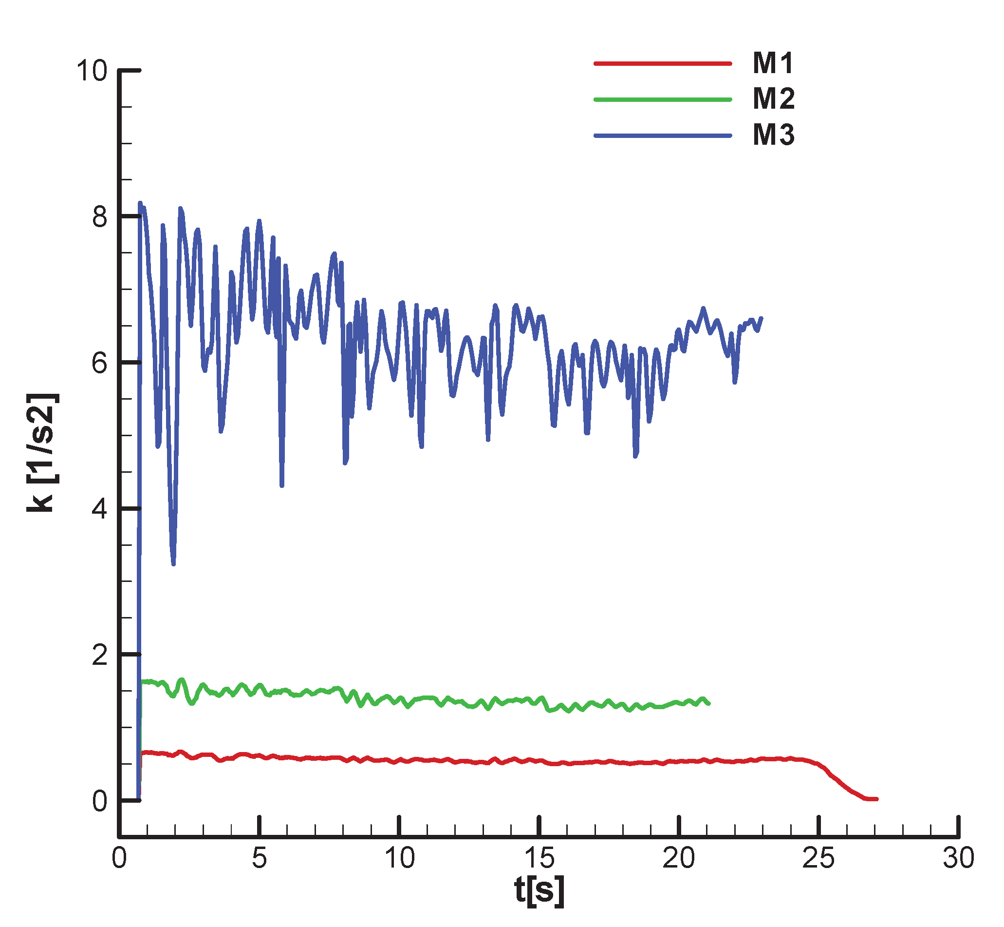
The objective of the nonlinear model analysis is to verify the limits of the guidance gain ( set out in the previous point, such as the guidance time We will consider parameters similar to linear analysis: and a tactical situation with a fixed target placed at a distance of 3 km and a height of 10 m. For the gain we will use the relation (91):
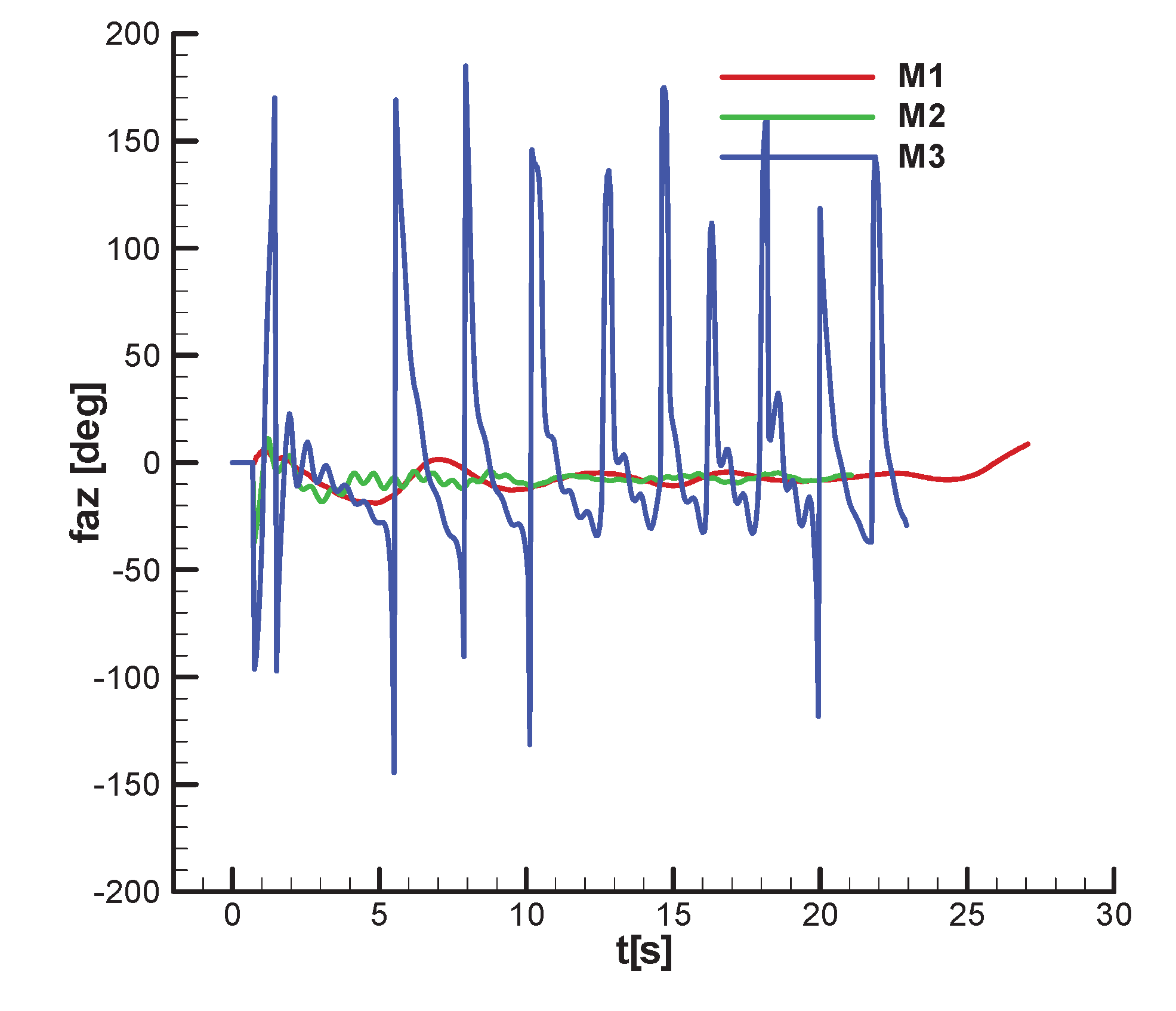
From this relation, only the first factor can be imposed because it is related to the constructive solution guidance device. At the same time, the second factor is constant and the third factor depends on the dynamics of the missile, being difficult to control. In this case, we will choose so that, when multiplied by the other two gains and velocity, a value close to the desired is obtained. Given the objectives of this section of the paper, we will seek to obtain three gains, the first less than the operating value the second close to the operating value , considerate optimal, and used in linear analysis, and the third bigger than the operating value, at the limit of the stability F-W range, as can be seen from Figure 29, namely . As previously stated, these values will be determined as a function of time, simultaneously with the integration of nonlinear equations of motion that will be done in the body frame. Obviously, due to the variation of the third factor , and the velocity the guidance gain will vary over time, as can be seen in and Figure 32 where the phase shift was . The analysis is performed considering three identical missiles but with different guidance gains, the first: M1, below the optimal value (the under-gain case), the second: M2 close to the optimal value defined in the linear analysis (the optimal-gain case), and the third: M2 bigger than the optimal (the over-gain case).
Figure 31.
Guidance gain; ; ;
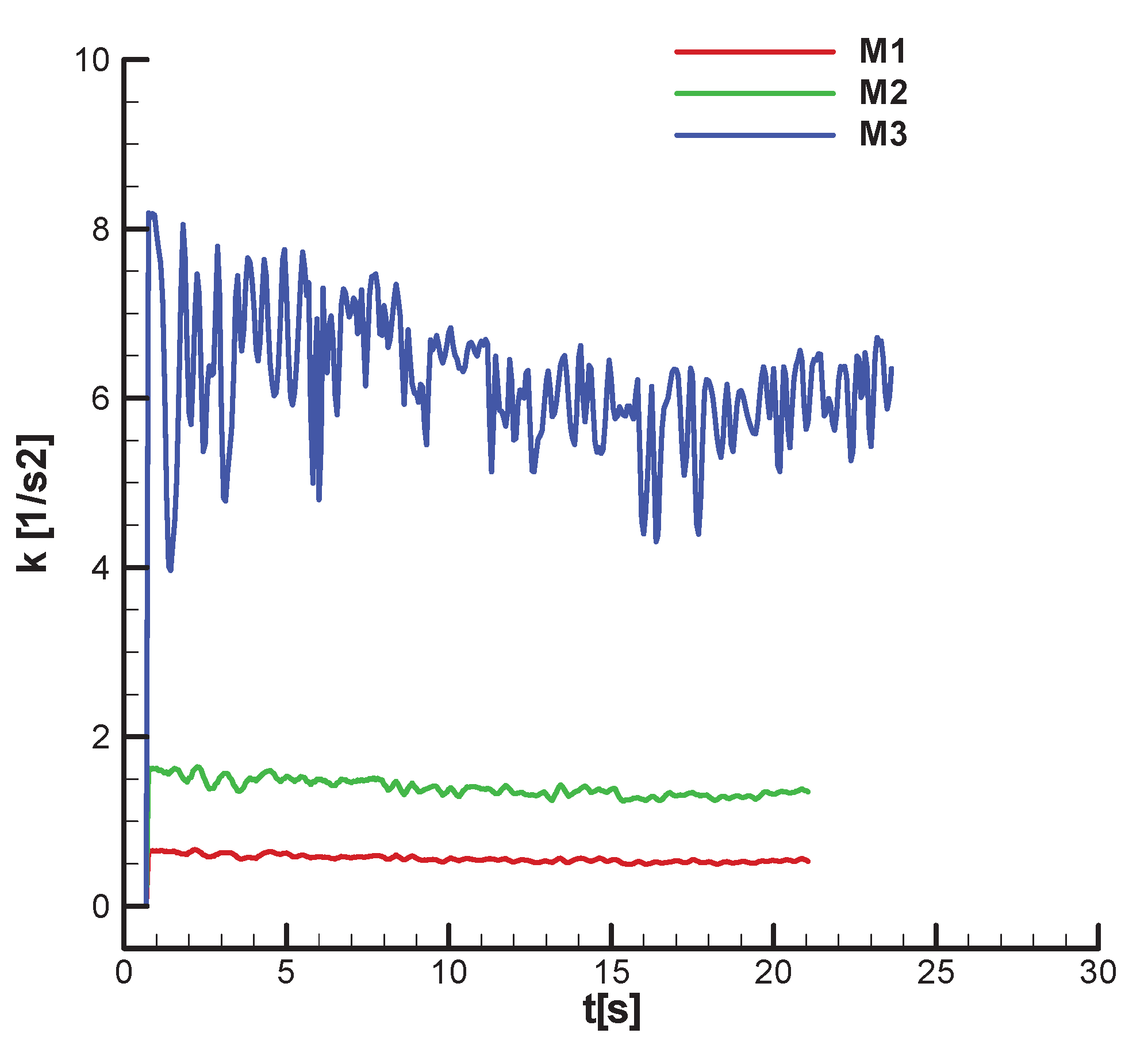
Figure 32.
Guidance gain; ; ;
For the three rocket models defined above Figure 33 and Figure 34 show the velocity diagram that was previously used to define the analysis range on the linear model , which corresponds to the second phase of flight. There are no significant differences between M1 and M2. For M3 (over-gain case), a loss of velocity is observed. This phenomenon occurs regardless of the phase shift, as can be seen from the two diagrams.
Figure 33.
Velocity diagram; ; ;
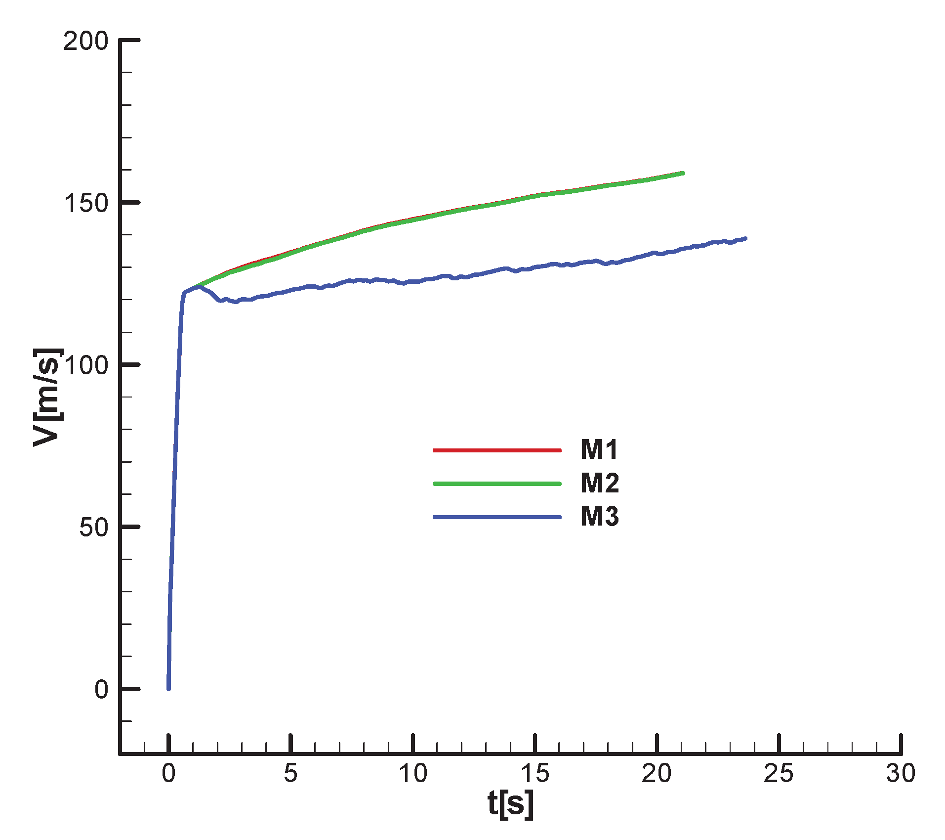
Figure 34.
Velocity diagram; ; ;
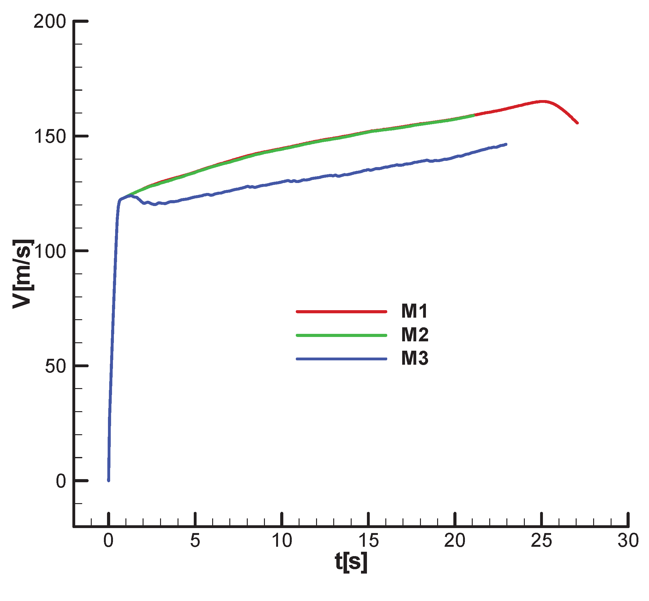
Figure 35 and Figure 36 show the angular roll velocity diagram based on which the rotational velocity of , corresponding to the second phase of flight, used in linear analysis, was chosen. It is observed that the roll velocity follows the velocity profile and does not differ substantially between M1 and M2. For M3 (over-gain case) a loss of roll velocity is observed. Similarly, for roll velocity, the phase shift does not have a significant influence.
Figure 35.
Roll velocity diagram; ; ;
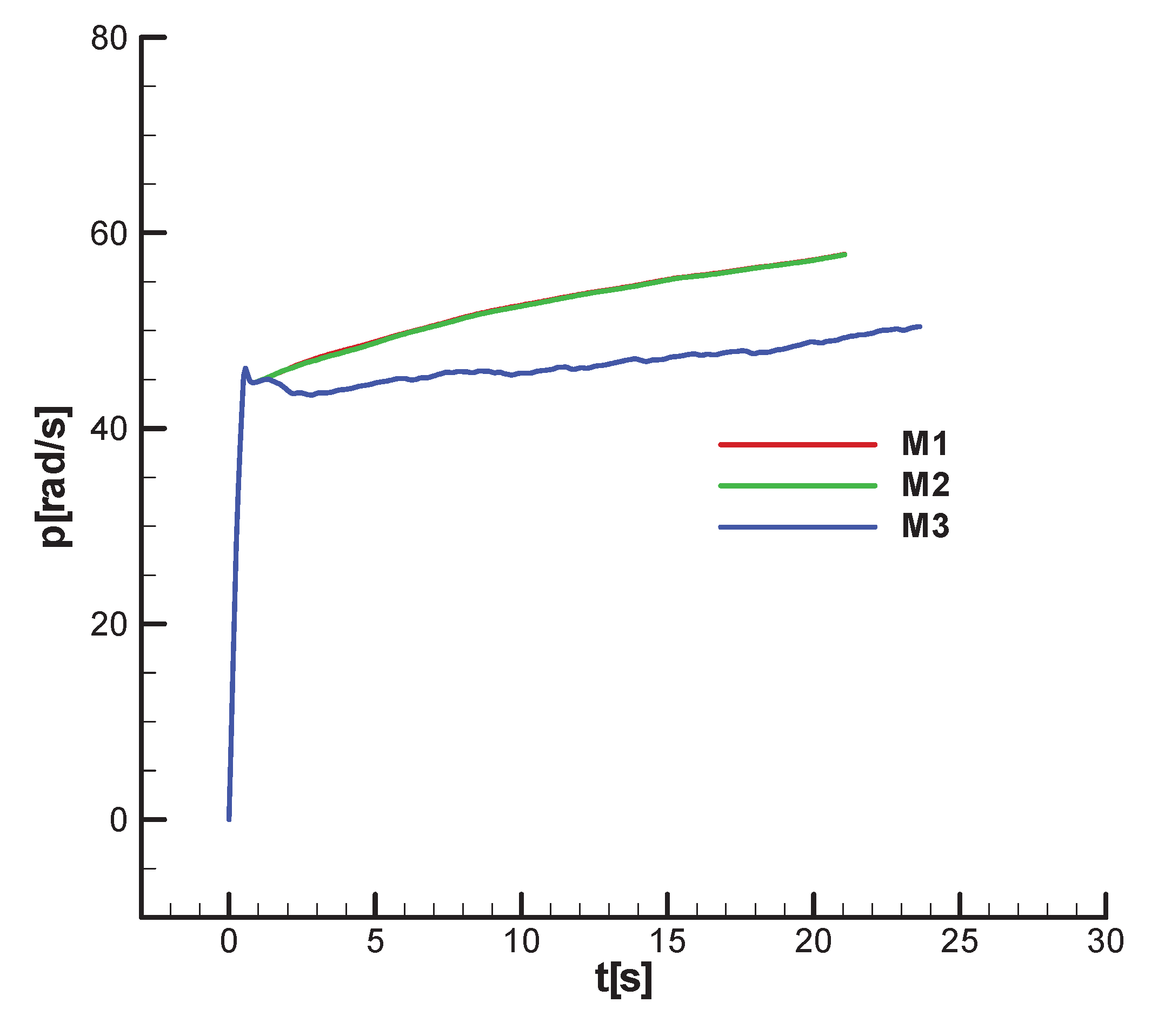
Figure 36.
Roll velocity diagram; ; ;
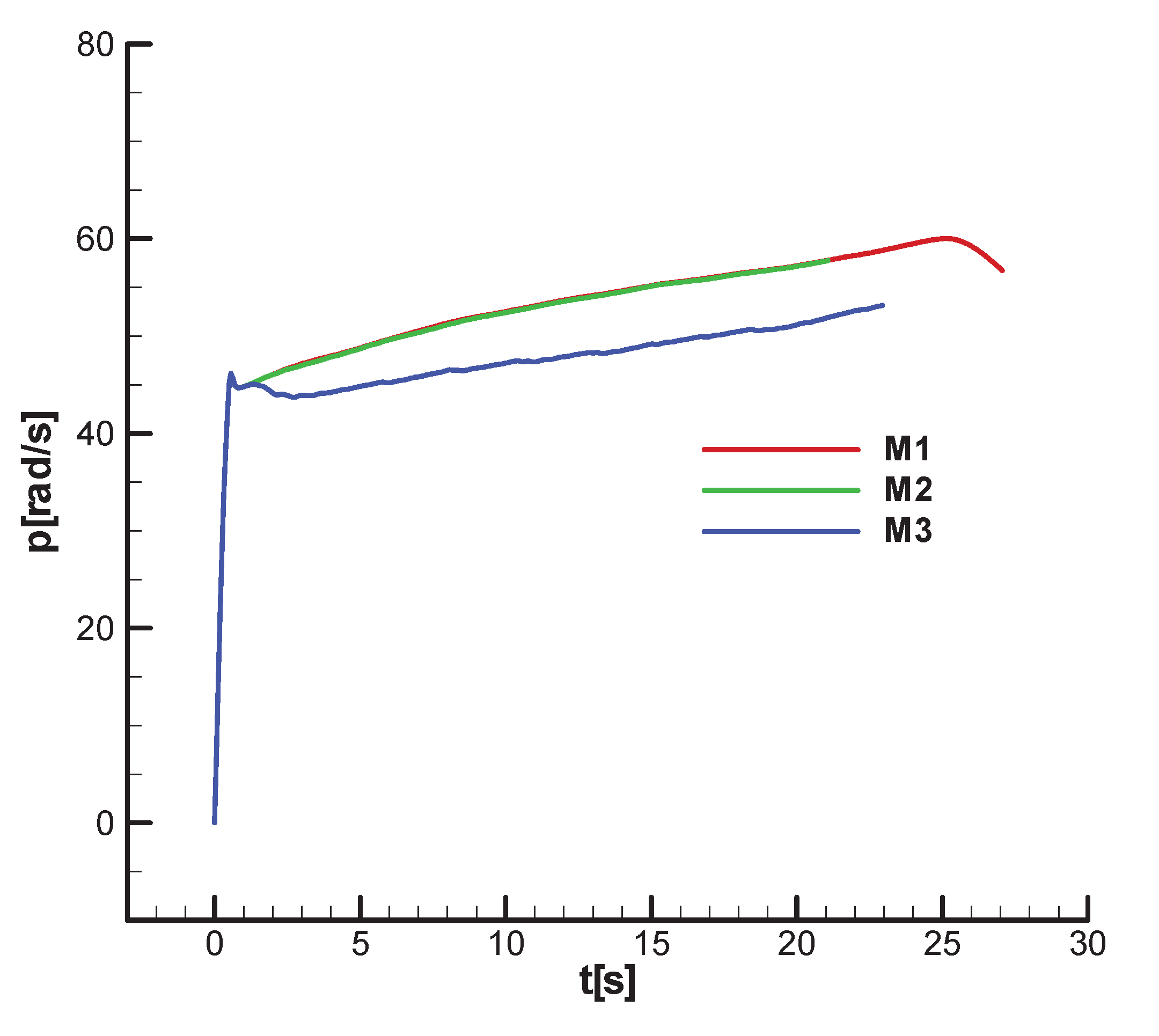
Figure 37 and Figure 38 show the vertical and horizontal projections of the trajectories for the three analyzed cases without the shift phase.
Observation: In the trajectory diagrams, the following were noted, according to [26]: A- carrier; T - Target; M – Missile.
Although all missiles hit the target, for M3 (the over-gain case), from vertical projection Figure 37 an overshoot can be seen at the entry into the second phase which caused the loss of velocity and roll velocity observed in the previous diagrams.
From the horizontal projection Figure 38, pronounced oscillations are observed for M3 (the over-gain), which can also lead to loss of velocity. Also, from both diagrams (the vertical and horizontal projection), it is observed that for M1, a greater final distance from the target is obtained but still within the imposed final distance of 3 m.
Figure 39 and Figure 40 show the vertical and horizontal projection of the trajectories for the three analyzed cases with shift phase (). Unlike the previously analyzed cases, if the shift phase is considered M1, with under-gain, it no longer reaches the target. The other features of the movement are preserved. For M3, an overshoot and oscillations along the trajectory are observed, which leads to a loss of velocity with a decrease in the performance of combating distant targets (over 3 km).
From the vertical projection (Figure 39) it can be seen that M1, after missing the target, continues to fly until it hits the ground.
From Figure 38 and Figure 40 a deviation of the trajectory to the left of the firing plane can be observed, a phenomenon specific to aerodynamically stabilized rolling missiles.
Figure 41 and Figure 42 show the command fill factor without and with the shift phase. It is observed that in both situations, for all missiles, the filling factor stabilizes at the equilibrium value, which achieves weight compensation. For both cases (Figure 41 and Figure 42), for M3, the filling factor saturates over a longer period of time, which leads to a decrease in the missile's maneuverability, therefore a decrease in performance, including the close targets. Also, for M3, strong oscillations are observed during the trajectory, which leads to a loss of velocity and, implicitly, a decrease in performance regarding distant targets. As for M1, it shows pronounced long-period oscillations of the filling factor, especially under shift phase conditions (Figure 42).
It is observed that in both situations, for all missiles, the phases stabilize at a small negative equilibrium value, which compensates for the Magnus and gyroscopic effects in the lateral plane.
For both cases, the phase of M3 has strong oscillations all the time, which leads to a loss of velocity, therefore a decrease in performance regarding distant targets.
Figure 45, Figure 47 and Figure 48 shows the influence of the guidance time . Unlike the cases previously analyzed, in these last situations, the three gain cases will be resumed, but with a reduced value of the guidance time .
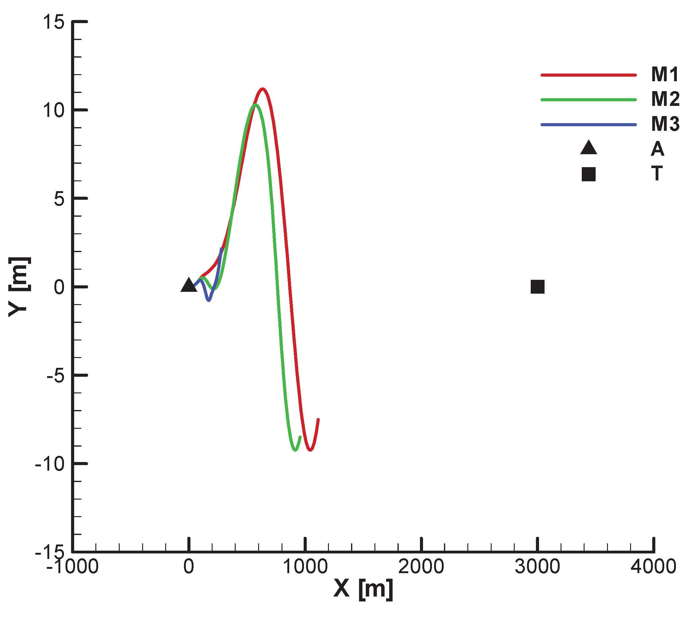
Thus, in Figure 45 and Figure 46 the vertical and horizontal projection of the trajectories for the case without the shift phase, and is presented. Let's compare it with the corresponding diagrams in Figure 36 and Figure 37 (with tau sub c equals 0.87). We can see that the decrease to leads to strong oscillations of the trajectory, which denotes a tendency to destabilase the system. In cases without the shift phase, M2 hit the target, while M1 and M3 missed the target. In contrast, for the cases with the shift phase (Figure 47 and Figure 48) with all three missiles miss the target, which shows the importance of a correct choice of guidance parameters.
Figure 45.
Target hitting – vertical view; ;
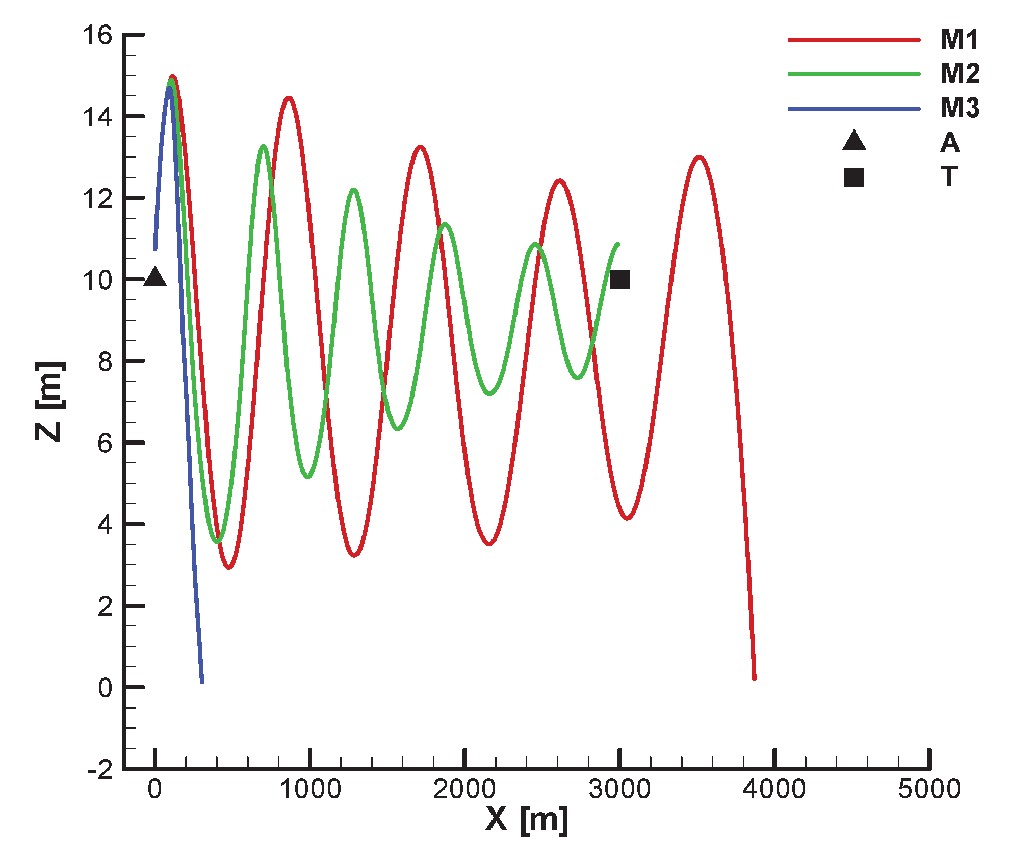
Figure 46.
Target hitting – horizontal view; ;

Figure 47.
Target missing – vertical view; ;
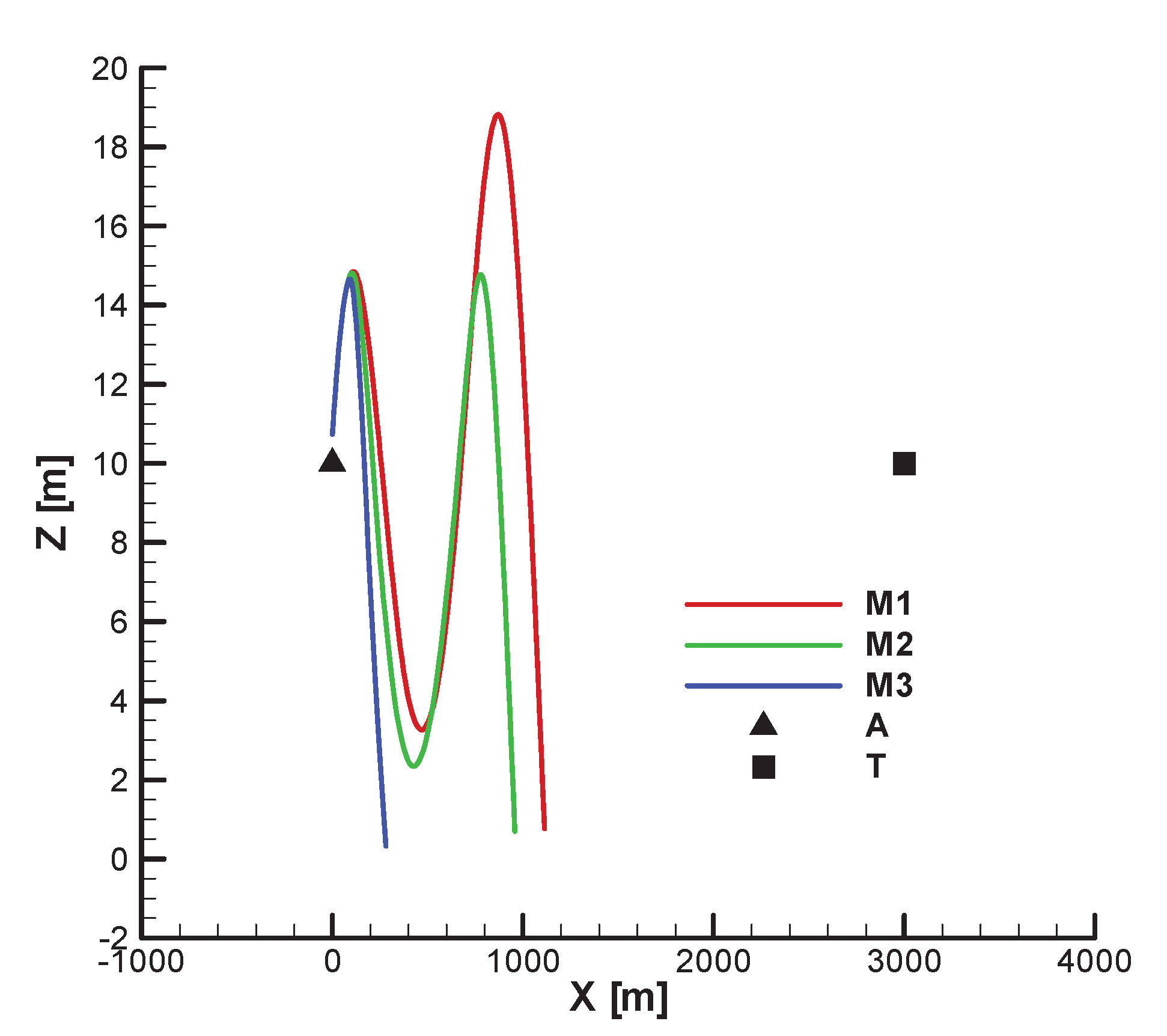
Figure 48.
Target missing – horizontal view; ;
8. Organization of Results from the Appendix
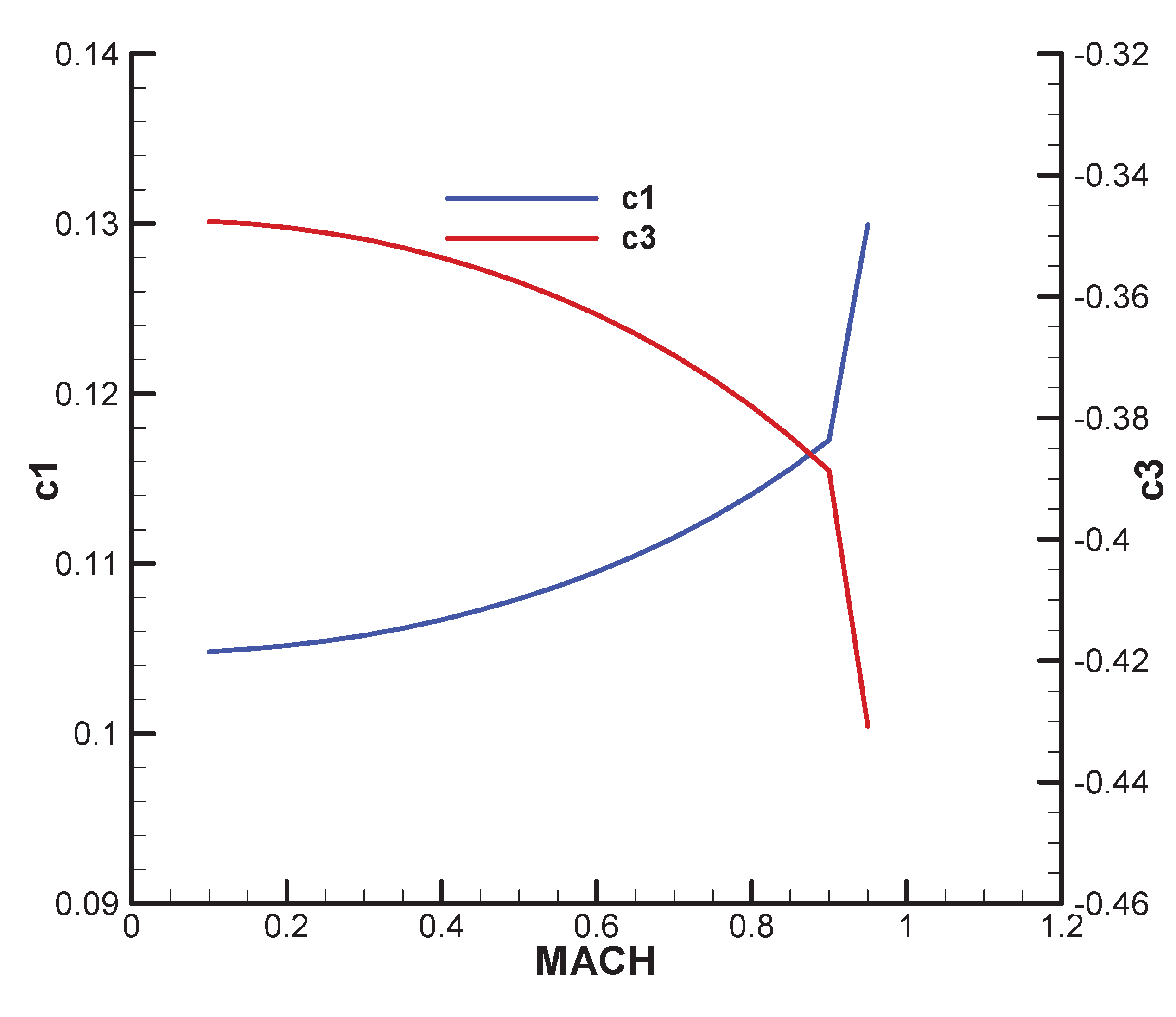
Appendix A illustrates the variation of the primary aerodynamic coefficients as a function of the Mach number.
Appendix B tabulates the thrust incidence, equilibrium thrust deflection angle, and key flight quality parameters for the start and end of the flight's second phase (marching mode), based on the mechanical data in Table 1. The analysis domain, selected with reference to the velocity profiles in Figure 33 and Figure 34, covers Mach numbers from 0.34 to 0.45 within the operational flight altitude.
The characteristic polynomial coefficients were determined for the start and end of the second flight phase using the relation (82) and the flight parameters from Appendix B. From these coefficients and relations (E 5), (E 6)(E 6),(E 7), the Frank-Wall (F-W) parameters ( were calculated as a function of the Mach number. As shown graphically in Appendix C, the results confirm the F-W stability criterion. , is met, with the positivity of the parameters demonstrated in Figure C9, Figure C10, Figure C11 and Figure C12.
Appendix D contains the root locus of the characteristic polynomial in both cases with real coefficients and complex coefficients.
Appendix E contains the algorithm details for Frank-Wall stability criterion for 5th order polynomials.
9. Conclusions
We present a stability analysis for a slowly rolling, single-channel Semi-Automatic Command to Line-of-Sight (SACLOS) missile. The analysis begins in Section 2 with the definition of the basic motion for a single-channel slow-rolling rocket with gasodynamic command. Next, in section 3, the coupled linear form of the commanded motion of the rolling missile was obtained.
Leveraging the missile's symmetric configuration, the analysis first identifies the symmetrical and cross-coupling terms for the pitch and yaw channels, treating the latter as complex quantities. Building on this, Section 4 derives the flight quality parameters and presents a structural model for the commanded motion of the rolling missile, which is characterized by complex parameters due to the inherent channel coupling.
Subsequently, Section 5 constructs the complete guided flight model. The development begins by defining the guidance kinematics and proceeds to a detailed analysis of the single-channel actuator, including its command generation logic and error compensation methods. The formulation of the final guidance equations integrates these components into the non-linear 6-DOF framework, creating a comprehensive guided flight model.
To complete the linear analysis, the commanded motion model from Section 4 is connected with the transfer functions for the guidance device and actuator within a closed guidance loop, yielding the final closed-loop structural diagram for the SACLOS system. Within this scheme, three parameters are emphasized, specifically the guidance gain. , the guidance time () and the time constant (), that will be analyzed in the following sections. Also, in Section 5, we obtained the characteristic polynomial of the transfer function associated with the closed-loop scheme. Next, based on the simplified structural scheme, a synthesis of the parameters of interest was carried out through a poly-zeros allocation method: “Standard coefficient method”.
Because in stability analysis from the following sections, we will use numerical values, in section 6, a numerical model was defined for a similar rocket in this class, for which aerodynamic, mechanical, thrust, time constants and amplification constants were provided, including the values for the guidance gain , the guidance time () and the time constant ().
Section 7, dedicated to stability analysis, contains three parts. First, it is dedicated to a simplified analysis using the R-H criterion for the characteristic polynomial with real coefficients. The second is the complex analysis using the F-W stability criterion for the characteristic polynomial with complex coefficients, and the third is for a realistic 6DOF model. The results obtained were compared between the three models, resulting in significant similarity between the linear model with complex coefficients and the nonlinear model. The presence of complex-valued elements in the system's structural scheme results in a characteristic polynomial with complex coefficients. Consequently, stability was assessed using the Frank-Wall (F-W) criterion, a generalization of the Routh-Hurwitz (R-H) criterion applicable to such polynomials. For the resulting 5th-order characteristic polynomial, the F-W criterion requires five distinct parameters to be positive to ensure system stability. Due to the analytical complexity of these F-W parameters, a simplified case was first considered where the missile's roll was neglected. This simplification enabled the use of the standard R-H criterion, yielding determinants with much simpler expressions. The subsequent analysis of these five R-H parameters resulted in the definition of five corresponding system constraints. Thus, from the first condition R-H resulted the first lower limitation for the time constant , the second condition for regular case with damping factor subunitary ( and the time constant of nutation positive is always fulfilled. The third condition resulted in an upper limitation for the guidance gain , and the fourth condition imposed a lower and the upper limit of the guidance gain ) more restrictive than the third condition. Also, a fifth condition imposes a lower limit for the guidance time .
The simplified Routh-Hurwitz (R-H) analysis yielded a fifth, more restrictive constraint on the time constant (τ>0). While the R-H parameters were treated analytically, the more complex Frank-Wall (F-W) parameters required numerical evaluation (Section 7). This numerical study included evaluating the F-W stability parameters and the influence of key parameters on the system's characteristic roots. A key finding from comparing the R-H (non-rolling) and F-W (rolling) results is that roll motion contracts the stable range for the guidance gain, particularly at the upper boundary. Finally, the linear F-W stability predictions were verified through non-linear simulations of a tactical scenario. Three cases were tested: under-gained (M1), optimal-gained (M2), and an over-gained case (M3) set at the predicted stability limit.
The results of the nonlinear model confirmed the limitations obtained with the F-W stability criterion. In the first and last cases, the system performance is degraded, for the first case (the under-gain case) obtains a greater final distance from the target, with the possibility of missing the target and for the third case, having large oscillations of the guidance parameters (phase and fill factor) during the flight. Moreover, for the third case, a significant overshoot is observed in the initial phase, which, together with the oscillations along the way, leads to a loss of velocity, with the loss of the ability to combat targets at long distances. Instead, in the second case, with the guidance gain close to the operating value, the missile hit the target, the guidance parameters having an asymptotic behavior during the trajectory. In parallel with the guidance gain, the behavior of the missile in the conditions of decreasing the guidance time from 0.87 [s] to 0.3 [s], for the three cases that were analyzed, finding that decrease leads to strong oscillations of the trajectory, which denotes a tendency to destabilize the system. In cases without the shift phase, M2 hit the target, while M1 and M3 missed the target. In contrast, for the cases with a shift phase with all three missiles miss the target, which shows the importance of a correct choice of guidance parameters.
In summary, this paper develops a comprehensive stability analysis for a slowly rolling, single-channel SACLOS missile, starting from a non-linear 6-DOF model formulated in the Resal frame. This model is first linearized to derive a structural scheme for the commanded motion, which yields flight quality parameters with a complex-valued form due to channel coupling. Subsequently, the guidance loop components—including the kinematic relations, guidance device, and a single-channel actuator with a specific switching function—are defined and linearized. These elements are then integrated to construct a complete, closed-loop linear model of the SACLOS system. From this linear model, the system's characteristic polynomial is determined. The presence of complex coefficients necessitates the use of the Frank-Wall (F-W) stability criterion, which is compared against the simpler Routh-Hurwitz (R-H) criterion for the non-rolling case. This analysis establishes a stability domain for the guidance gain and lower limits for the guidance time constant. A key finding is that the stability domain predicted by the F-W criterion (with roll) is more restrictive than that obtained with the R-H criterion. Finally, the results of the linear stability analysis are verified through simulation with the original non-linear 6-DOF model. The non-linear system's behavior shows strong agreement with the predictions of the more accurate F-W criterion, thus validating the derived stability boundaries for the guidance gain and time constant.
The paper contains five Appendixes, as follows: Appendix A presents graphical the main terms of development of aerodynamics coefficients; Appendix B presents graphical the linear model flight quality parameters used for the characteristic polynomial of the transfer function; Appendix C presents graphical the real and imaginary part of the characteristic polynomial coefficients as well as the five F-W stability parameters; Appendix D contain the root locus of the characteristic polynomial. Appendix E detailing the calculation of F-W stability parameters.
10. Nomenclature
Aerodynamics terms
;- Term of development of axial force coefficient
;- Terms of development of coefficients for normal forces
;- Terms of development of the torque coefficients in pitch and yaw
;
- Terms of development of the roll torque coefficient
The Flight Quality Parameters
– The natural pulsation of nutation;
– The damping factor of nutation;
– The time constant of nutation;
– The command factor;
– The advance time on command;
– The angular rate of precession;
– The static stability;
– The reference time;
– The reduced mass of the aircraft or relative density;
– The reduced moment of inertia in pitch;
– The reduced gravitational acceleration;
– The maximum load factor;
The Guidance Parameters
A – The Carrier;
M – The Missile;
T – The Target;
– Line of sight carrier-target;
AM – Line of sight carrier – missile;
– Range of the target related to the carrier;
– Range of the missile related to the carrier;
– Range of the target related to the missile;
– The attitude angles for the guiding frame orientation;
, - Absolute angles of the line of sight carrier - target;
, - Absolute angles of the line of sight carrier - missile;
– The angular deviations in guiding planes;
– The rate of angular deviations in guiding planes;
– The linear deviations in guiding planes;
– Missile climb angle and flight path azimuth angle;
– Missile velocity;
– The components of the missile velocity in the guiding frame;
– Target climb angle and flight path azimuth angle;
– Target velocity;
– The components of the target velocity in the guiding frame;
– Missile acceleration;
– Target acceleration;
, – Angular rate of LOS carrier- target;
, – Angular rate of LOS carrier- missile;
– Missile angular rates of the velocity vector;
– The guidance gain;
– The guidance time;
– The time constant;
– The guidance command in the body frame;
– The guidance command in the Resal frame;
– The command module;
– The command phase;
– The phase shift error;
– The fill factor;
– The relative roll angle;
– The pitch canard deflection angle;
– The average equivalent canard deflection;
– The guidance device gain;
– The actuator gain;
The Stability Parameters
– Routh- Hurwitz determinants
– Frank-Wall stability parameters
Appendix A. Aerodynamics
The reference system for all aerodynamic coefficients is the body frame.
The reference area, respectively the reference length for all aerodynamic coefficients, is the fuselage cross-section, respectively the fuselage length.
For torque coefficients, the reference point is the final center of mass of the rocket.
For the translational development terms, work [33] with experimental corrections was used.
For rotational and non-stationary terms, including Magnus terms, the paper [29] was used.
Figure A1.
Term of axial force coefficient at zero incidence (a1). Term of development of the coefficient of axial force with the squares of incidences (a2).
Figure A1.
Term of axial force coefficient at zero incidence (a1). Term of development of the coefficient of axial force with the squares of incidences (a2).
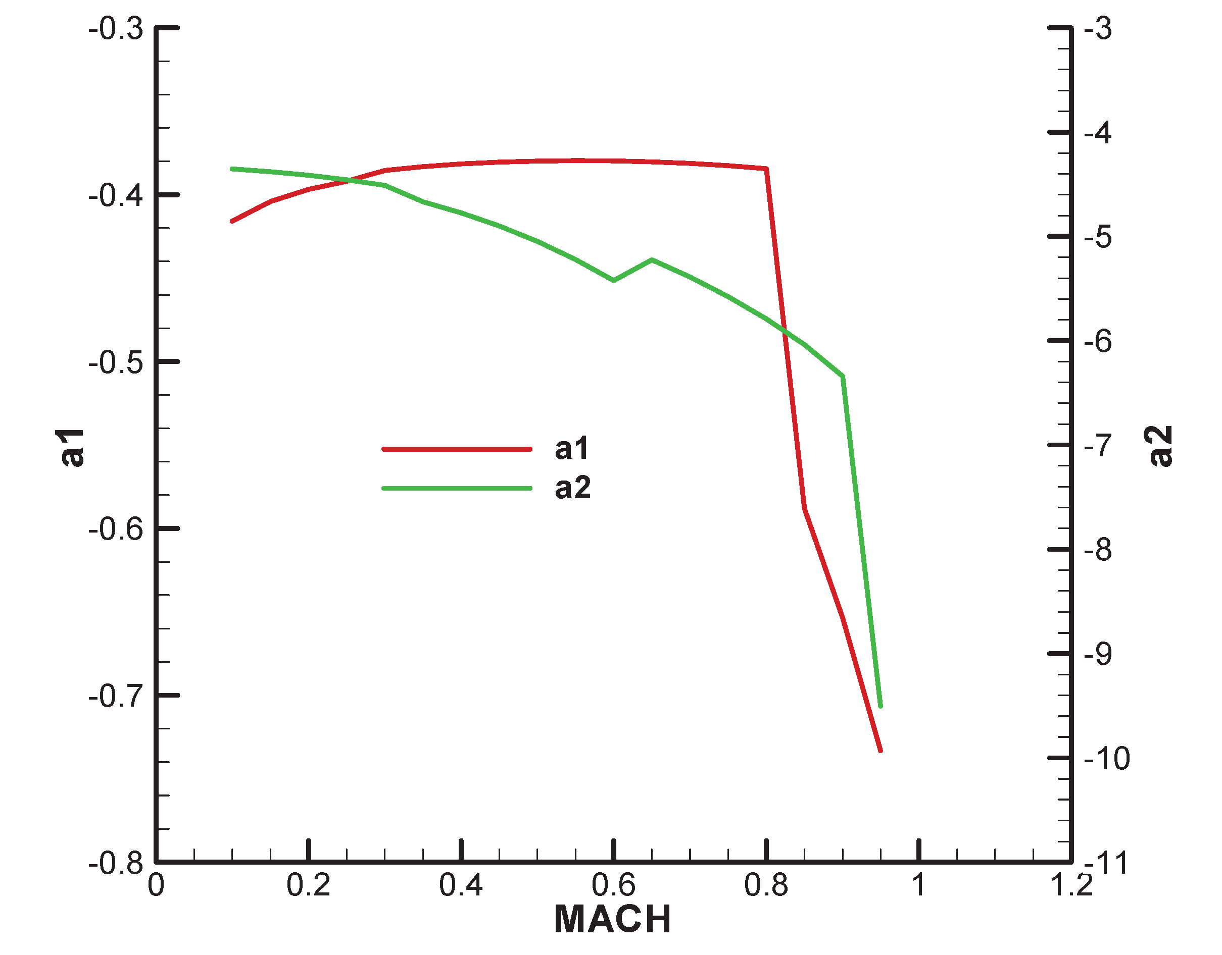
Figure A2.
Term of development of the coefficient of axial force with the incidence of the 4th power (a3). Term of development of the coefficient of axial force with the product of quadrat incidences (a4).
Figure A2.
Term of development of the coefficient of axial force with the incidence of the 4th power (a3). Term of development of the coefficient of axial force with the product of quadrat incidences (a4).
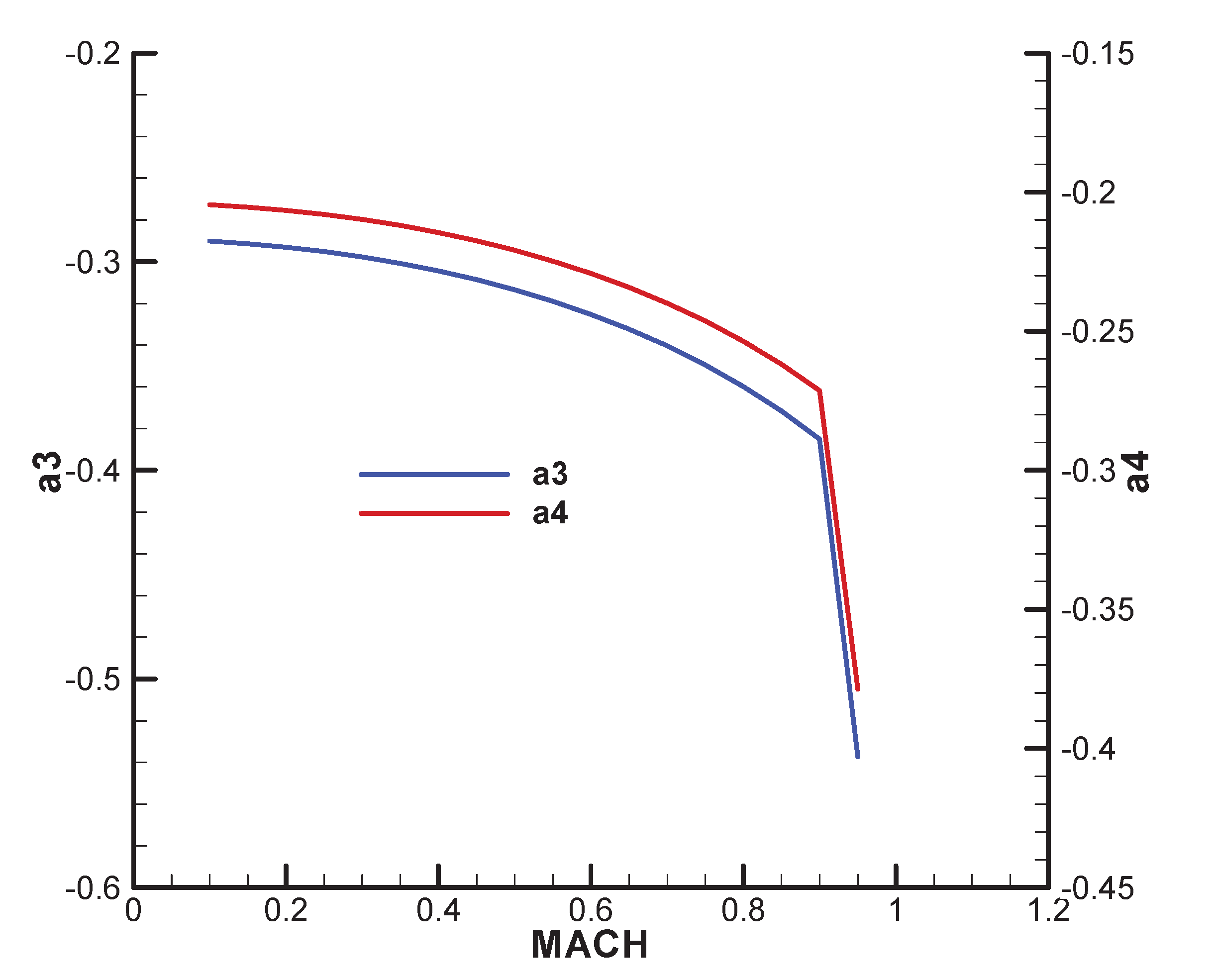
Figure A3.
Terms of development of coefficients for the normal forces with incidences.
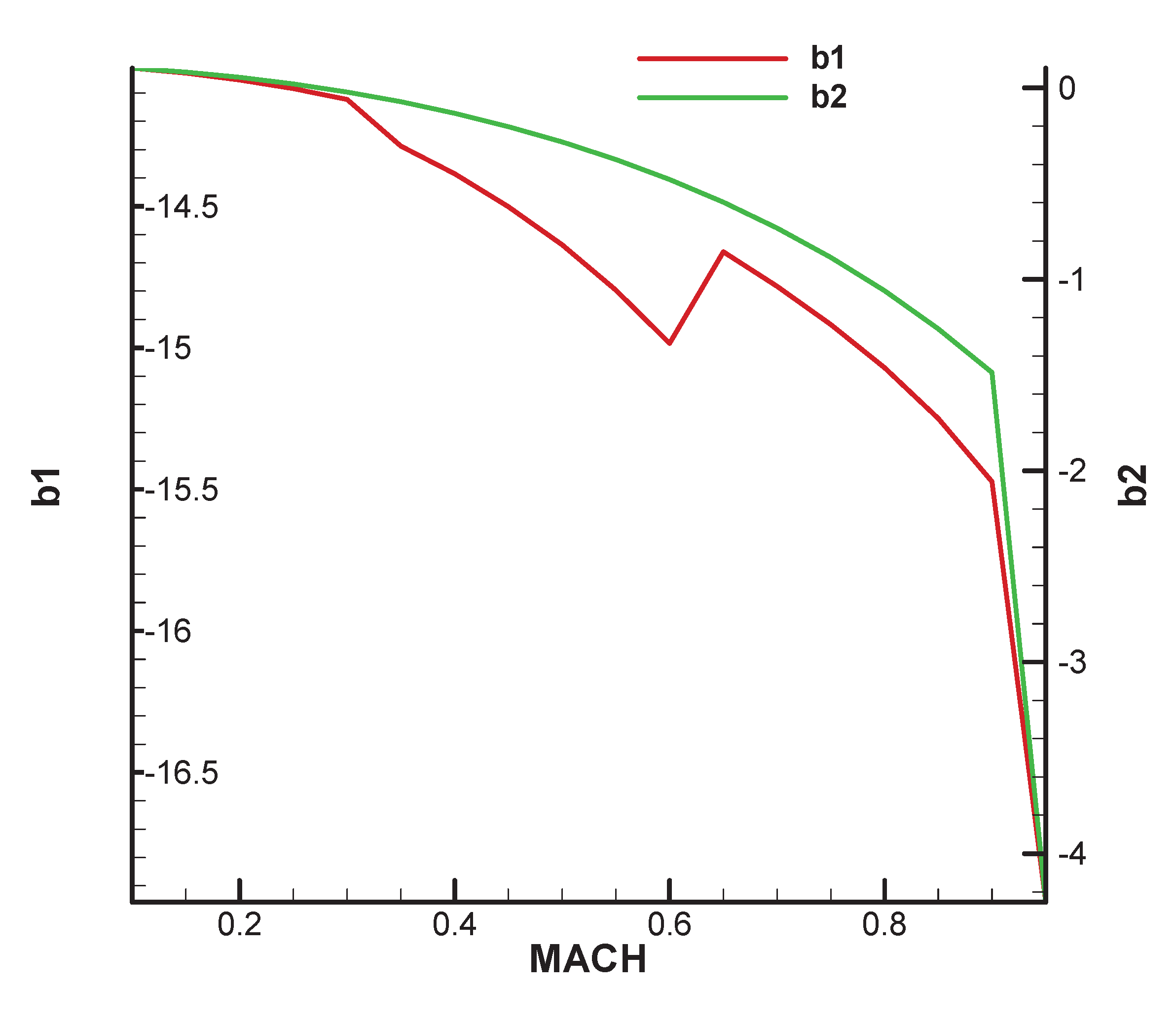
Figure A4.
Magnus terms of the development of coefficients for the normal forces.
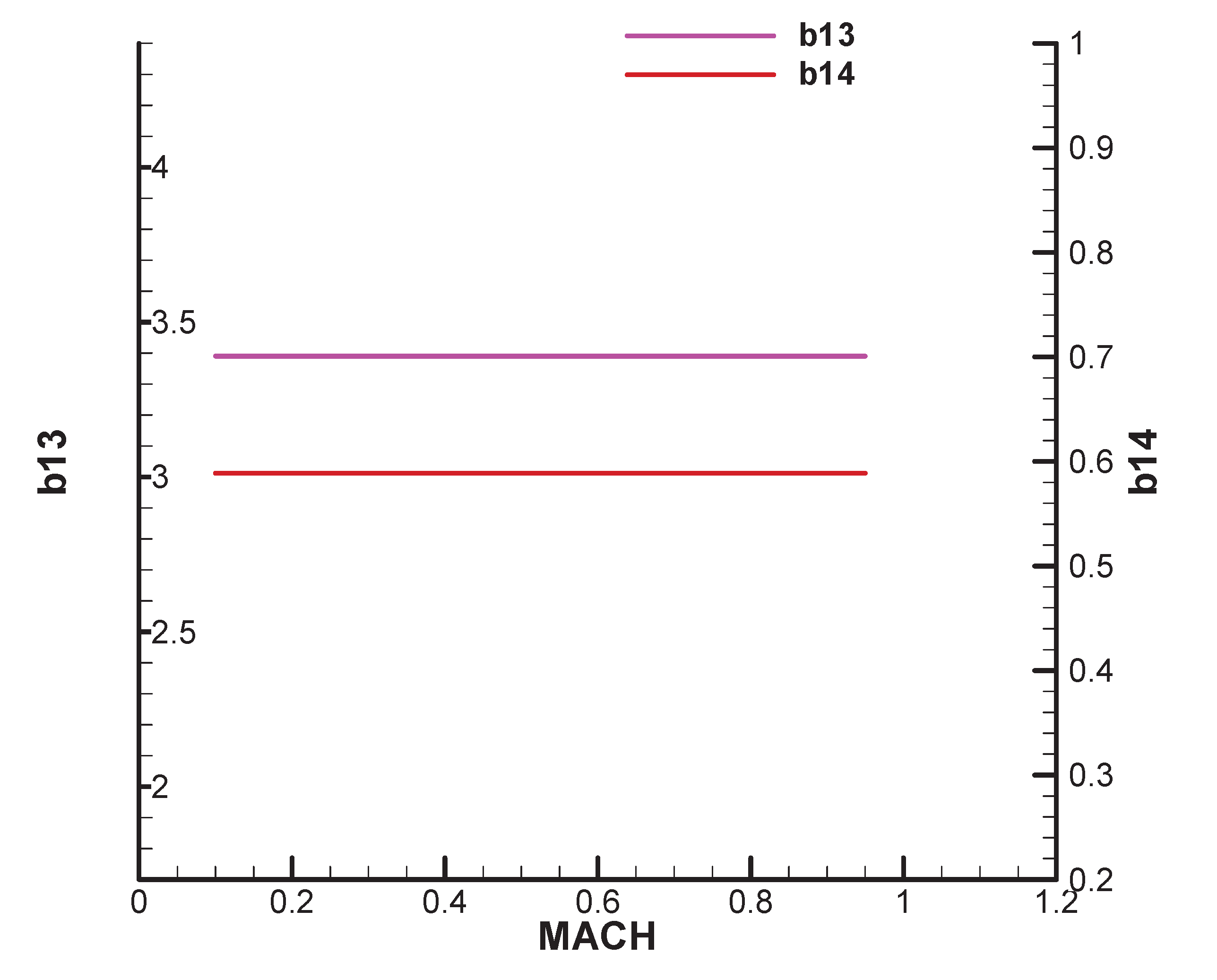
Figure A5.
Terms of development of coefficients of normal forces with rate of incidence (b9) and angular velocity (b4).
Figure A5.
Terms of development of coefficients of normal forces with rate of incidence (b9) and angular velocity (b4).
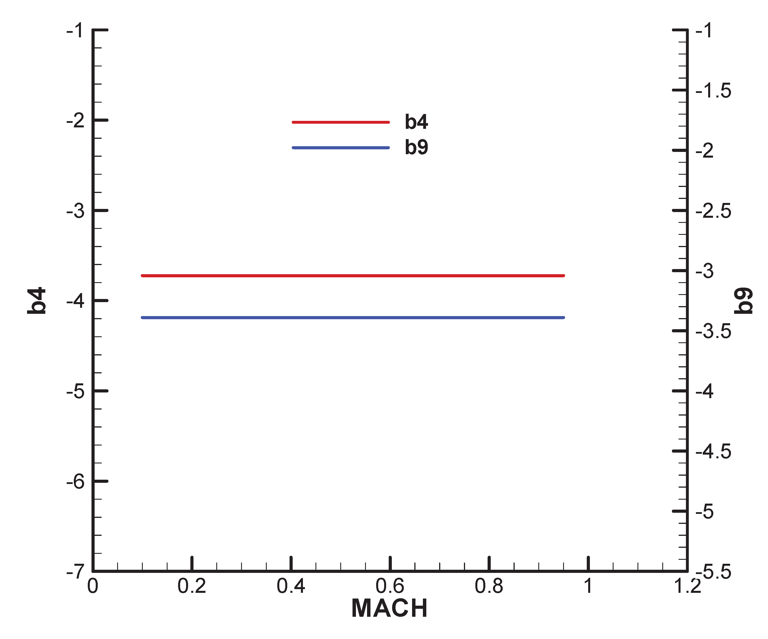
Figure A6.
Terms of development of the torque coefficients in pitch and yaw with incidences.
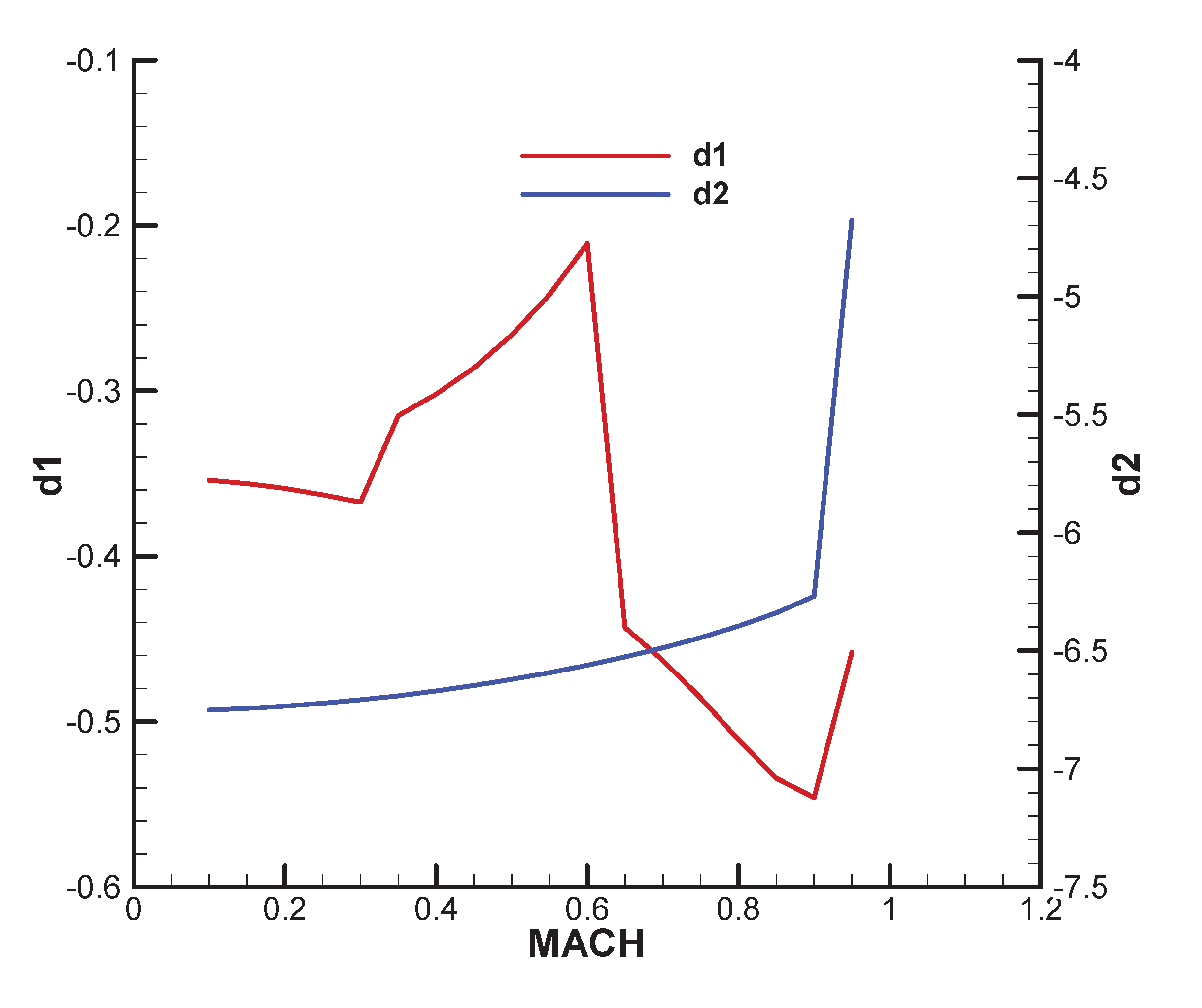
Figure A7.
Magnus terms of the development of pitch and yaw torque coefficients.
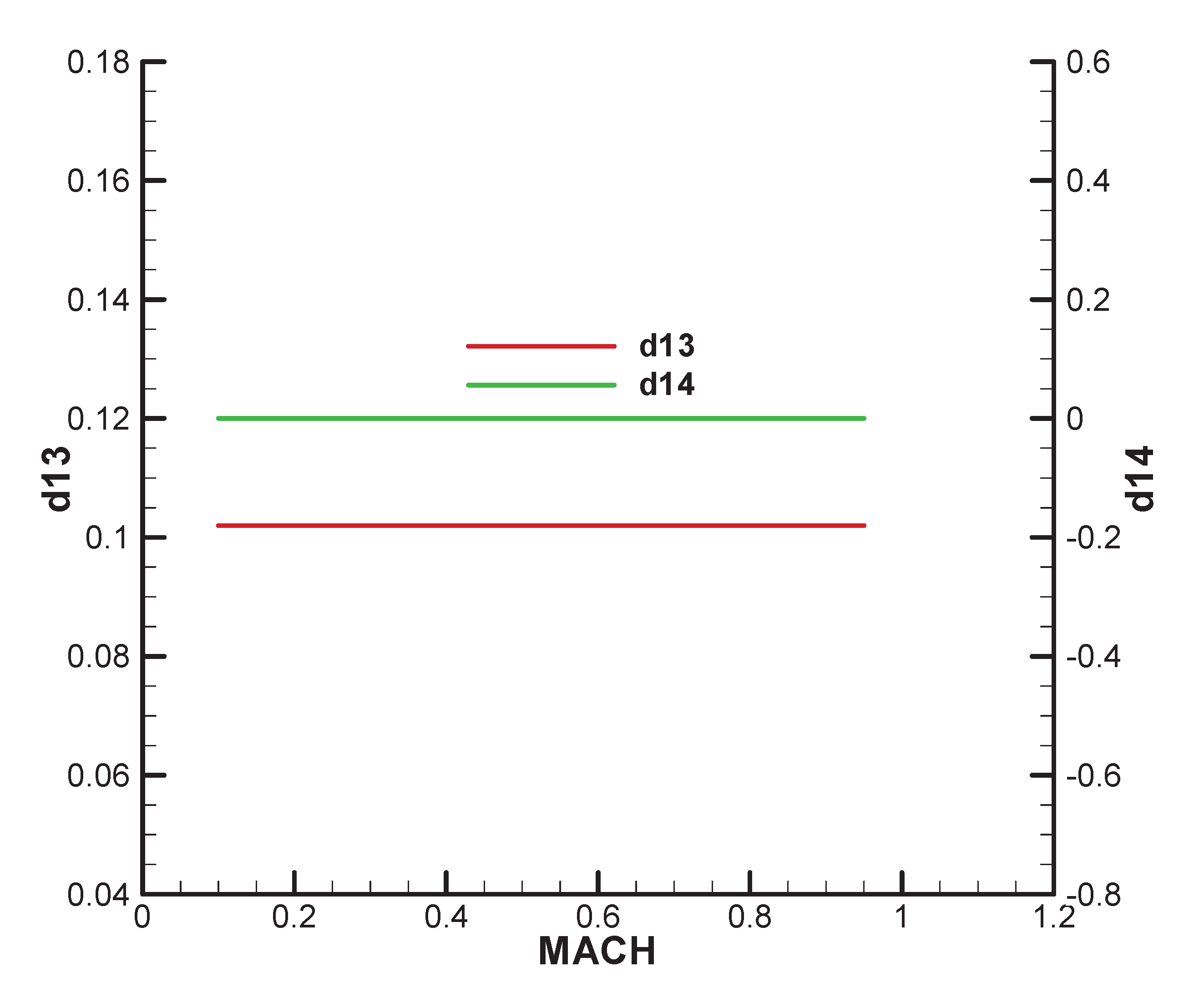
Figure A8.
Terms of development of the torque coefficient in pitch with rate of incidence (d9) and angular velocity (d4).
Figure A8.
Terms of development of the torque coefficient in pitch with rate of incidence (d9) and angular velocity (d4).
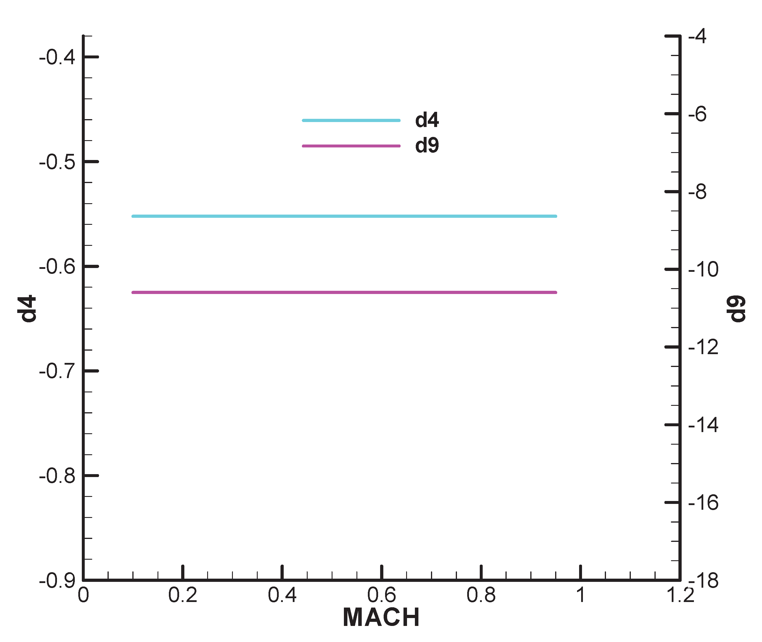
Figure A9.
Terms of development of the roll torque coefficient.
Appendix B. Parameters of the Linear Model
Basic Movement
Figure B1.
Velocity (V) and roll angular rate (p) corresponding to velocity.
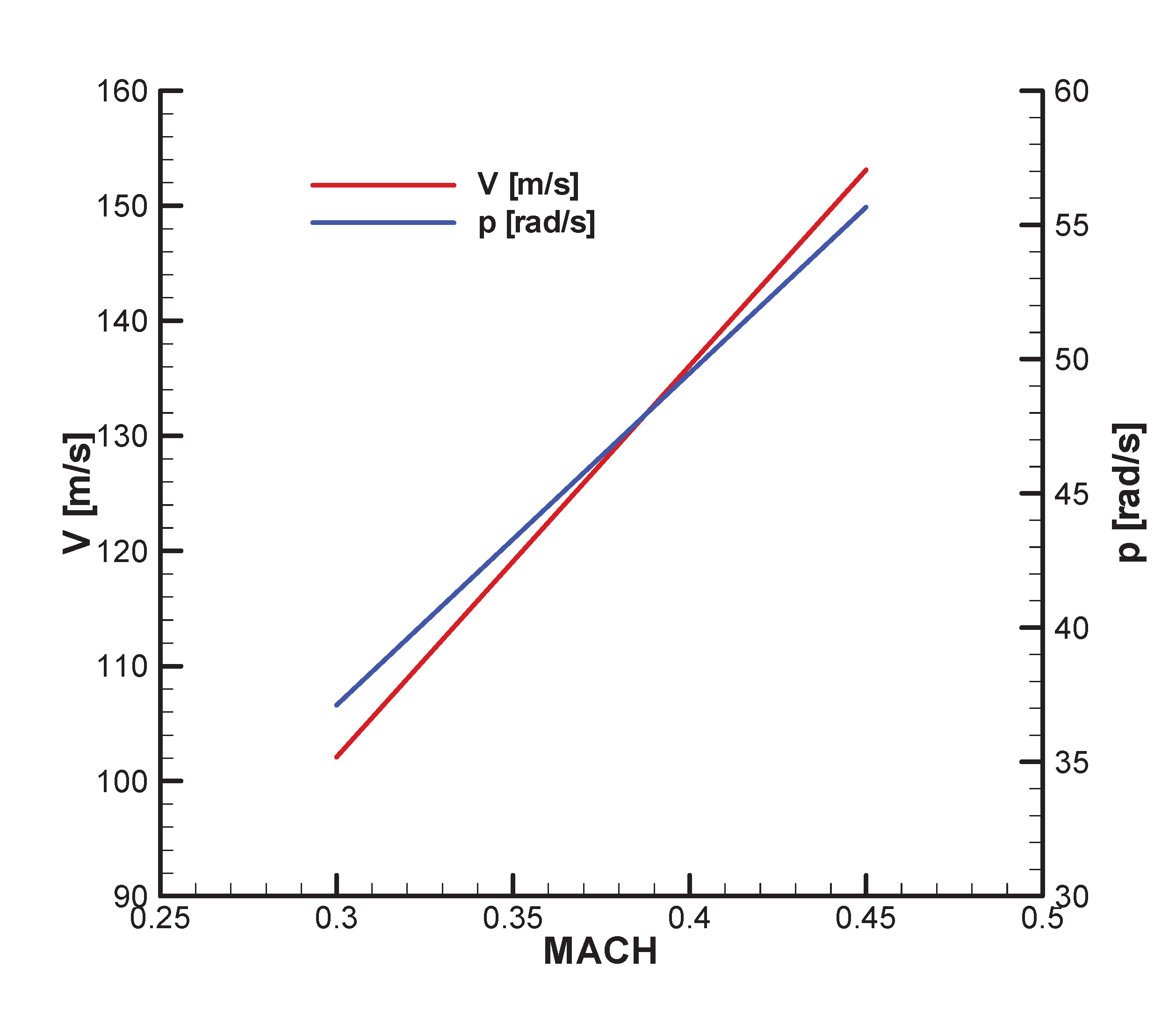
Figure B2.
Equilibrium incidence in the vertical plane.
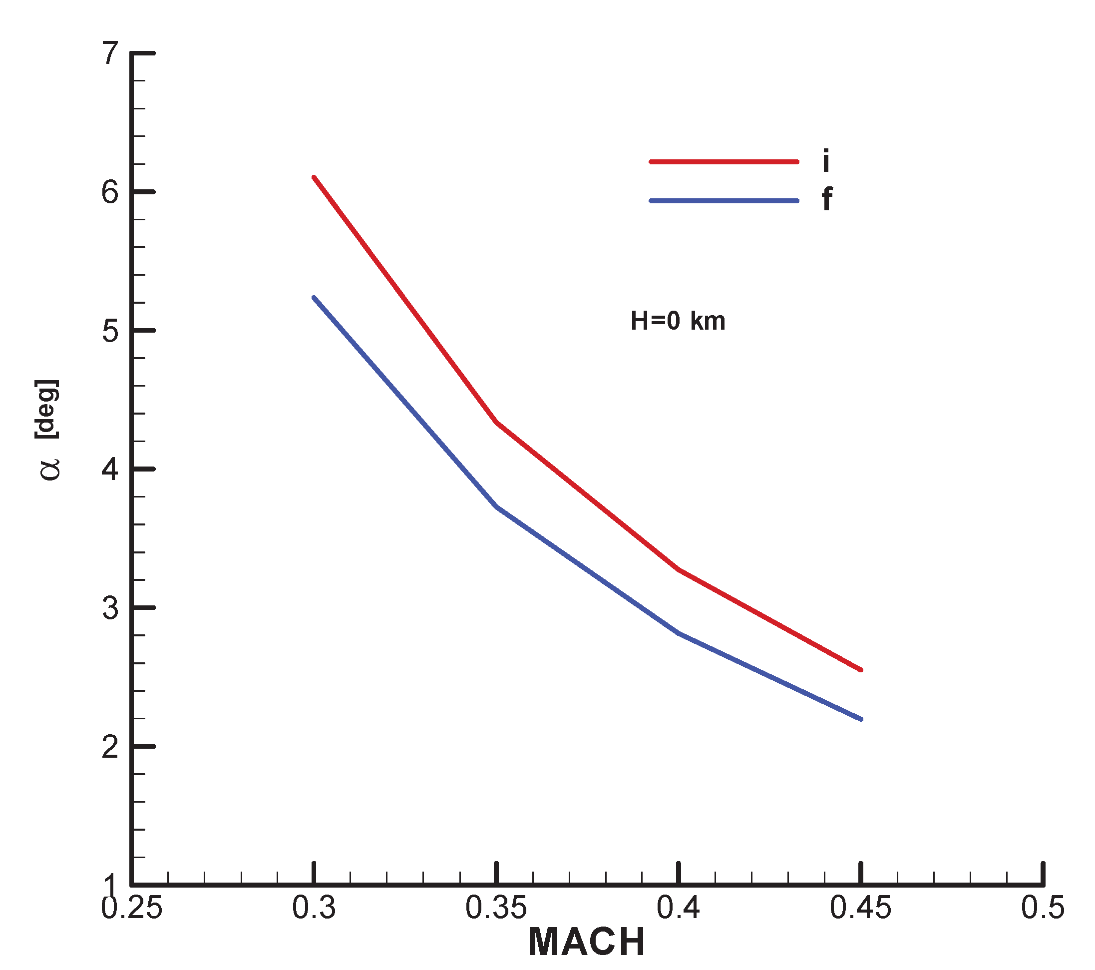
Figure B3.
Equilibrium pitch thrust deflection.

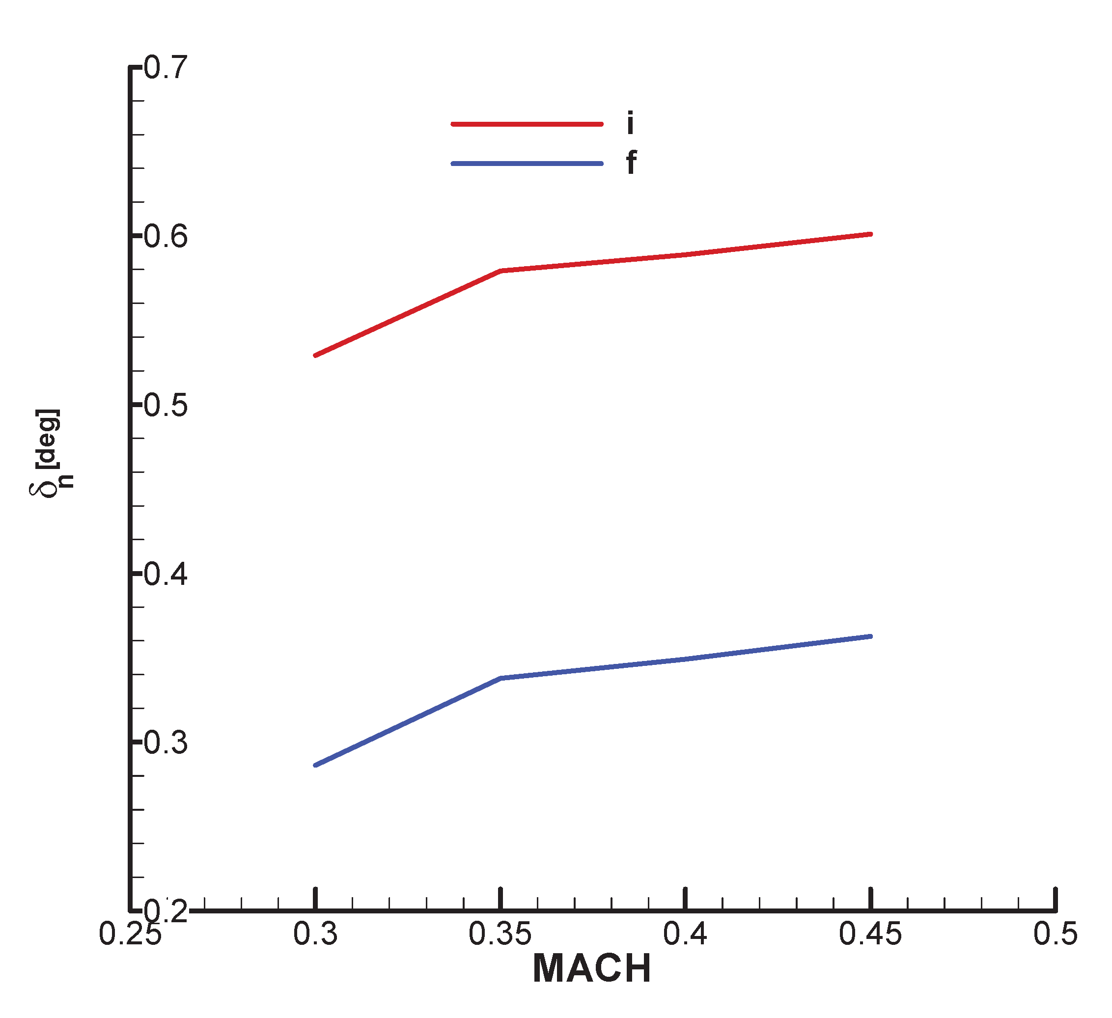
Figure B4.
Equilibrium yaw thrust deflection.
Stability Matrix
Figure B5.
Derivative term of the incidence equation against incidence.
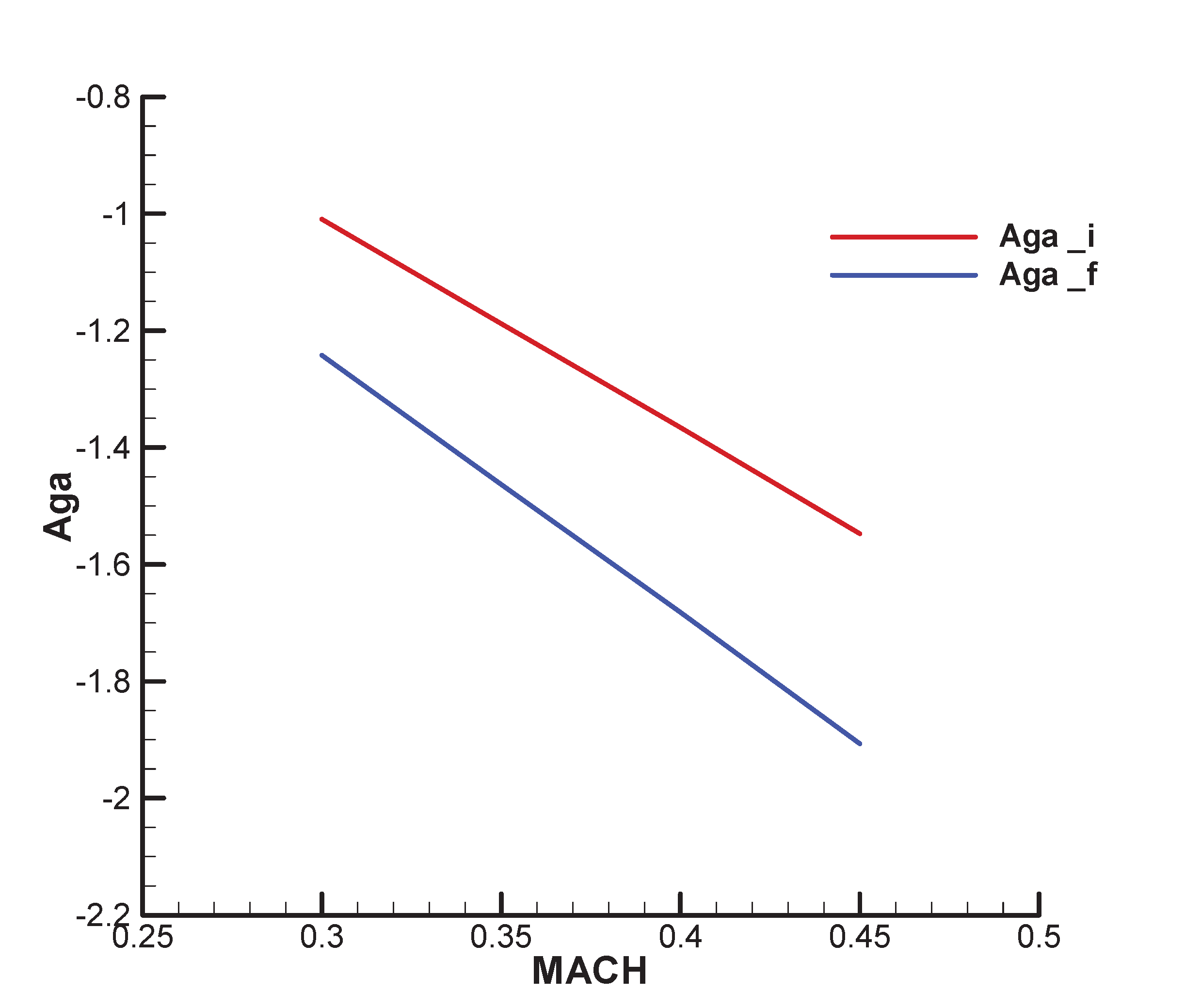
Figure B6.
Derivative term of the incidence equation against angular velocity.
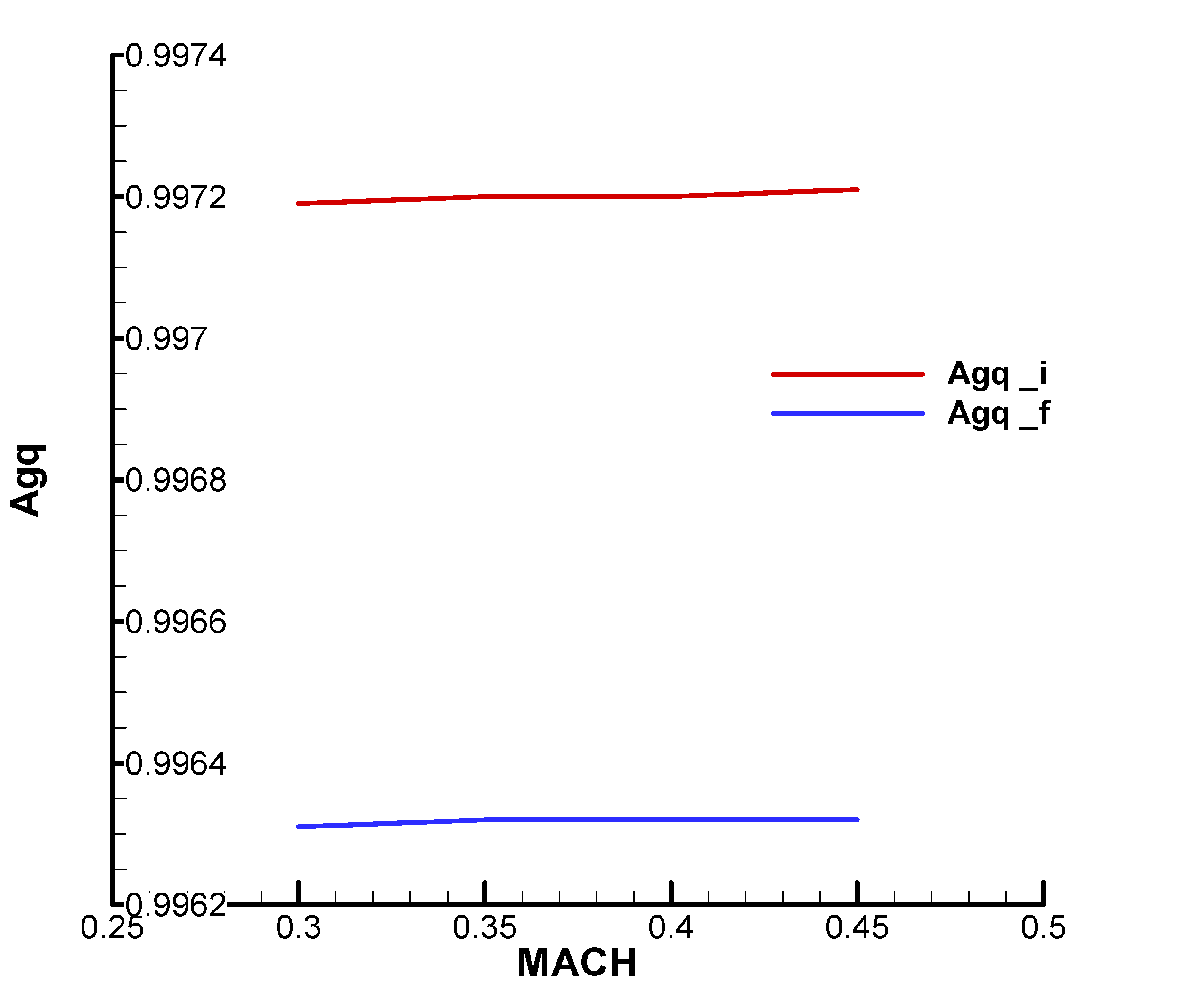
Figure B7.
Derivative term of the incidence equation against unsteady incidence.
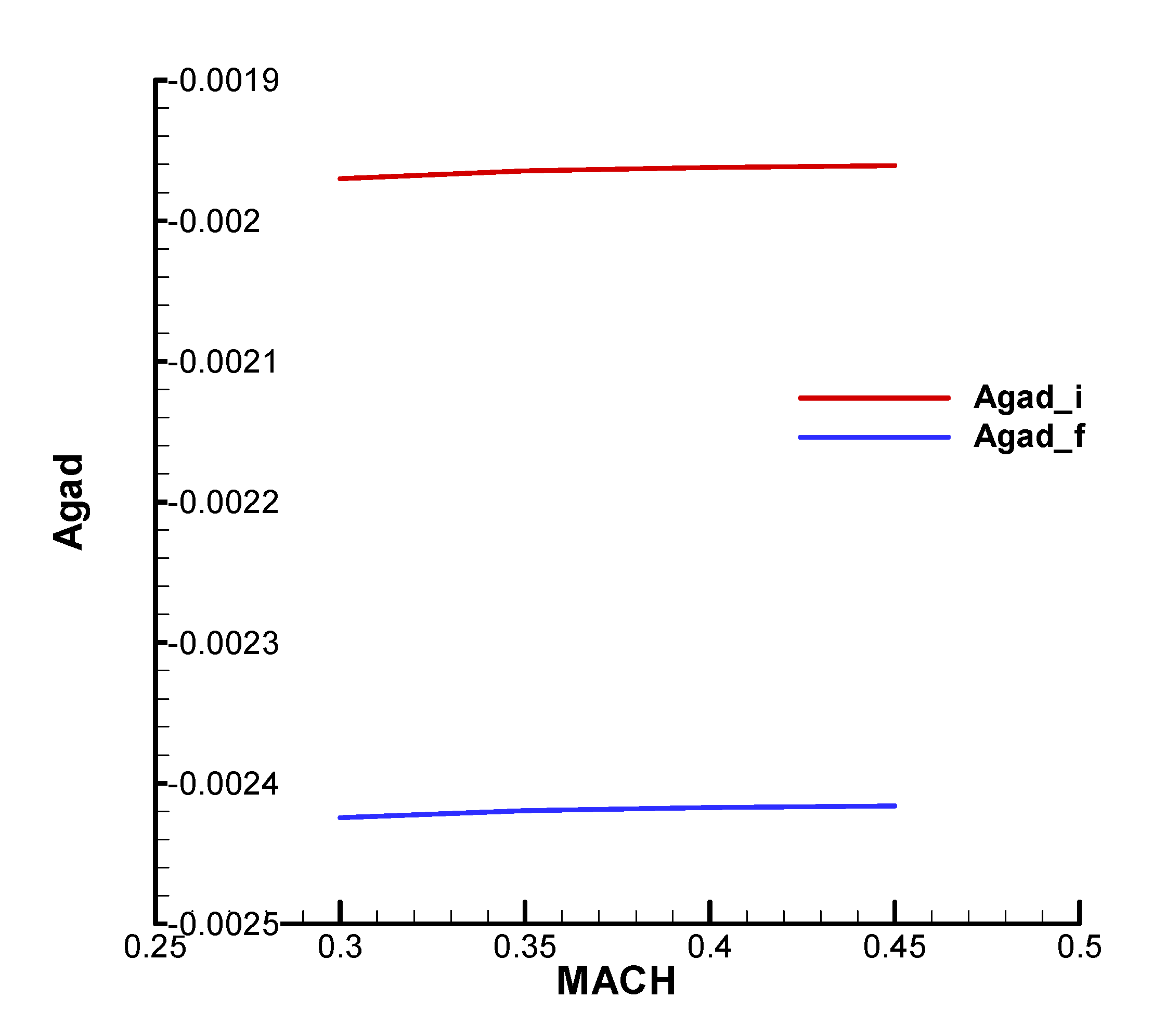
Figure B8.
Derivative term of the incidence equation against the cross incidence – Magnus term.
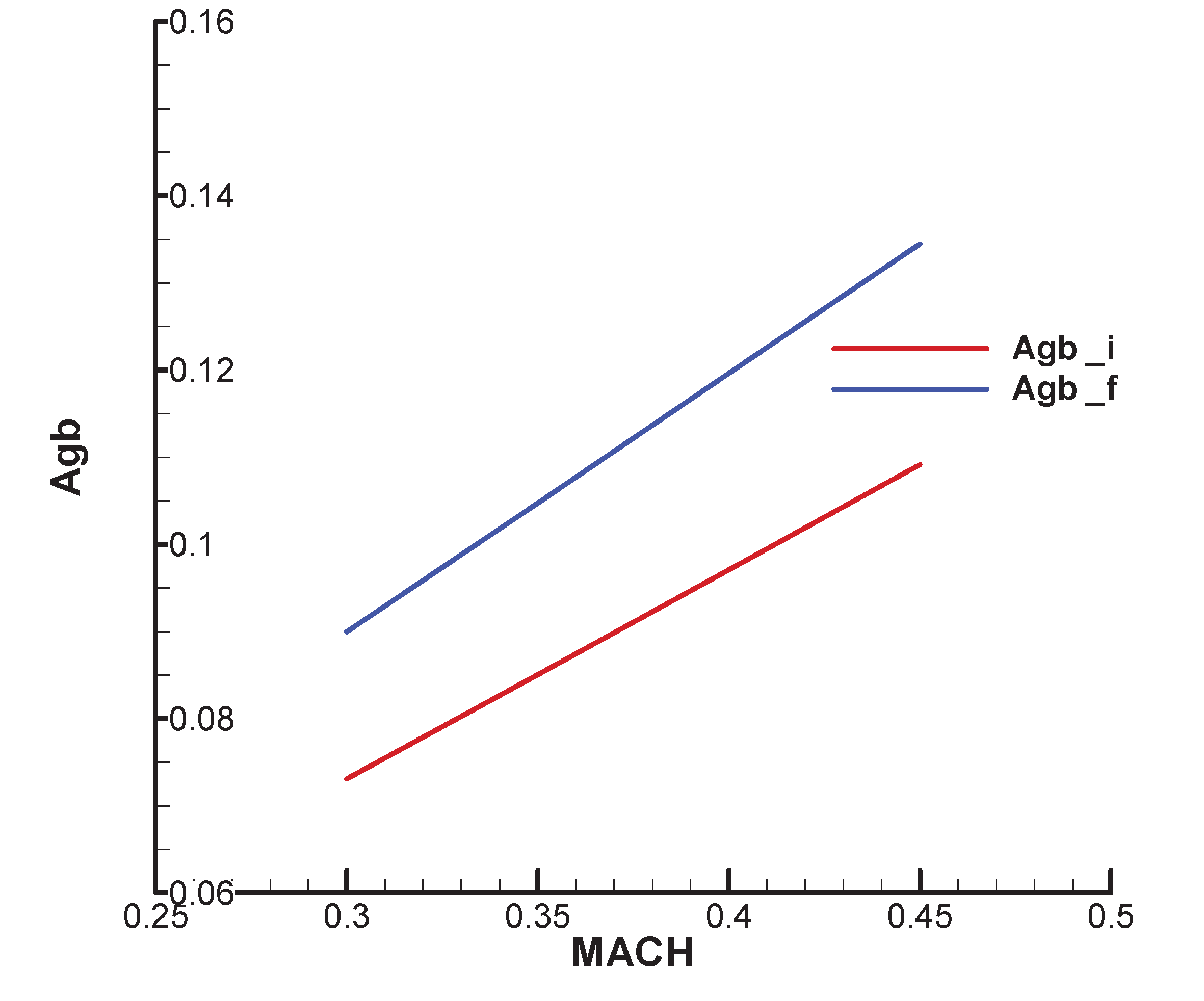
Figure B9.
Derivative term of the incidence equation against the cross angular velocity – Magnus term.
Figure B9.
Derivative term of the incidence equation against the cross angular velocity – Magnus term.
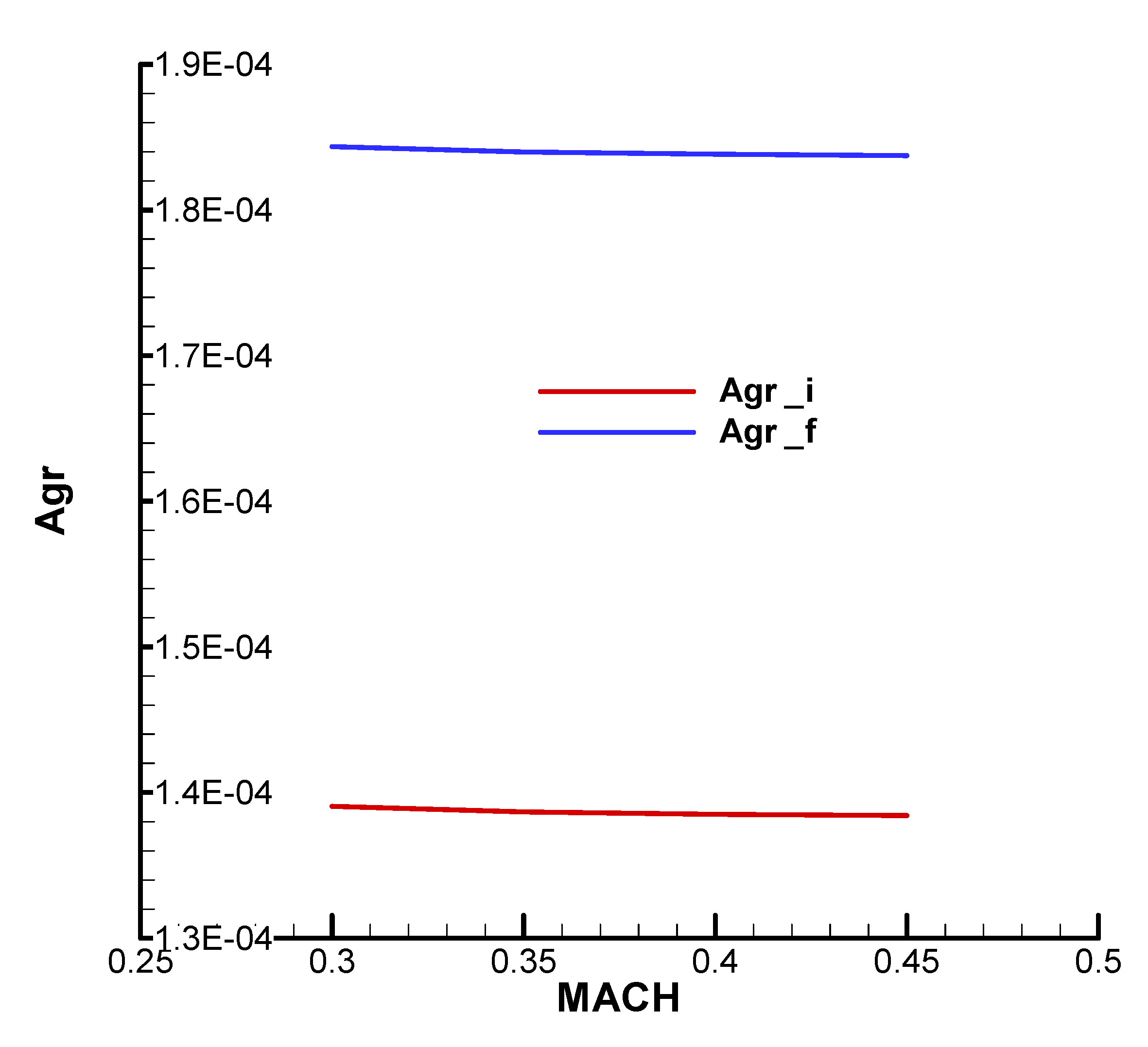
Figure B10.
Derivative term of the angular velocity equation against the incidence.
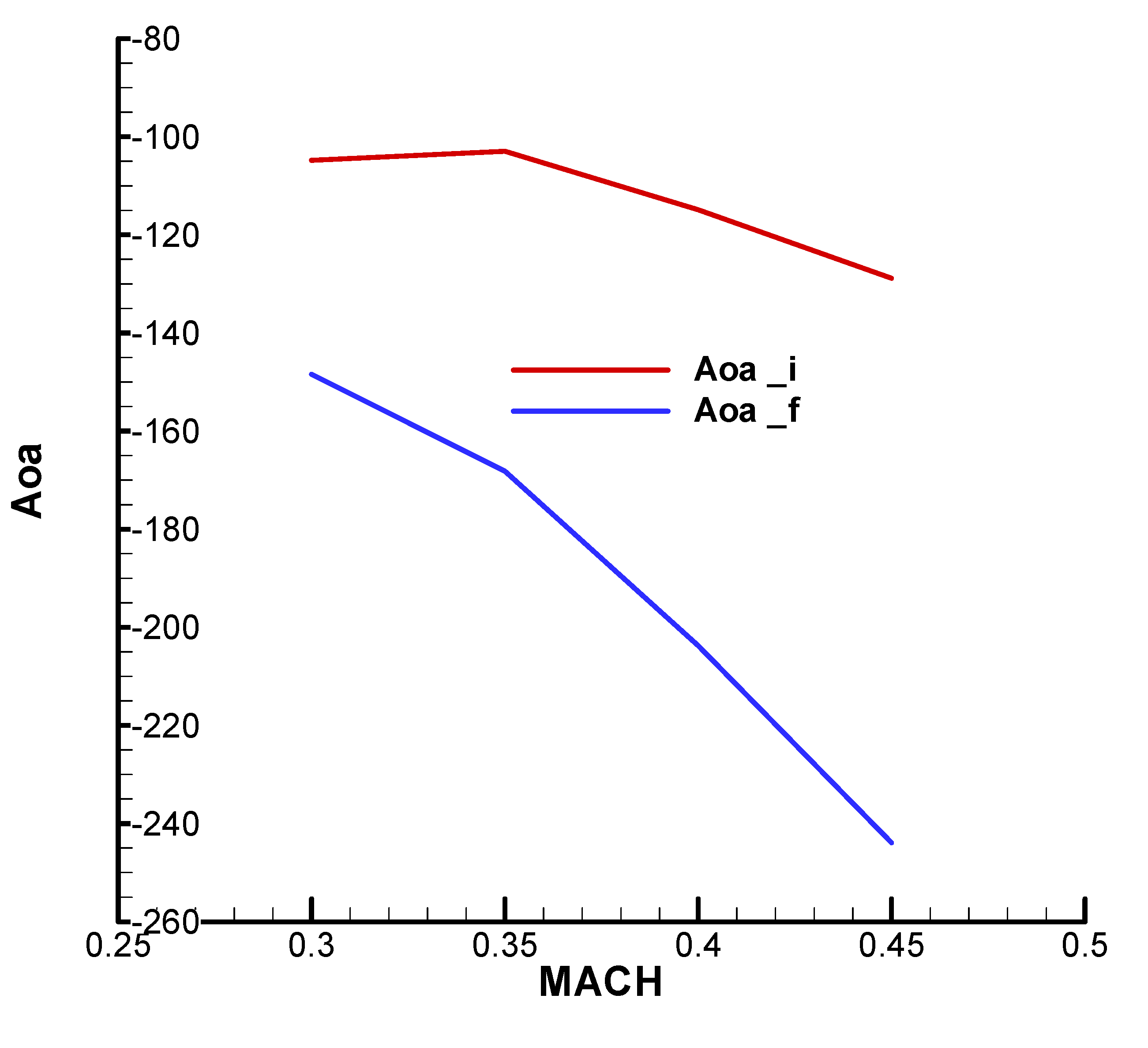
Figure B11.
Derivative term of the angular velocity equation with respect to angular velocity.
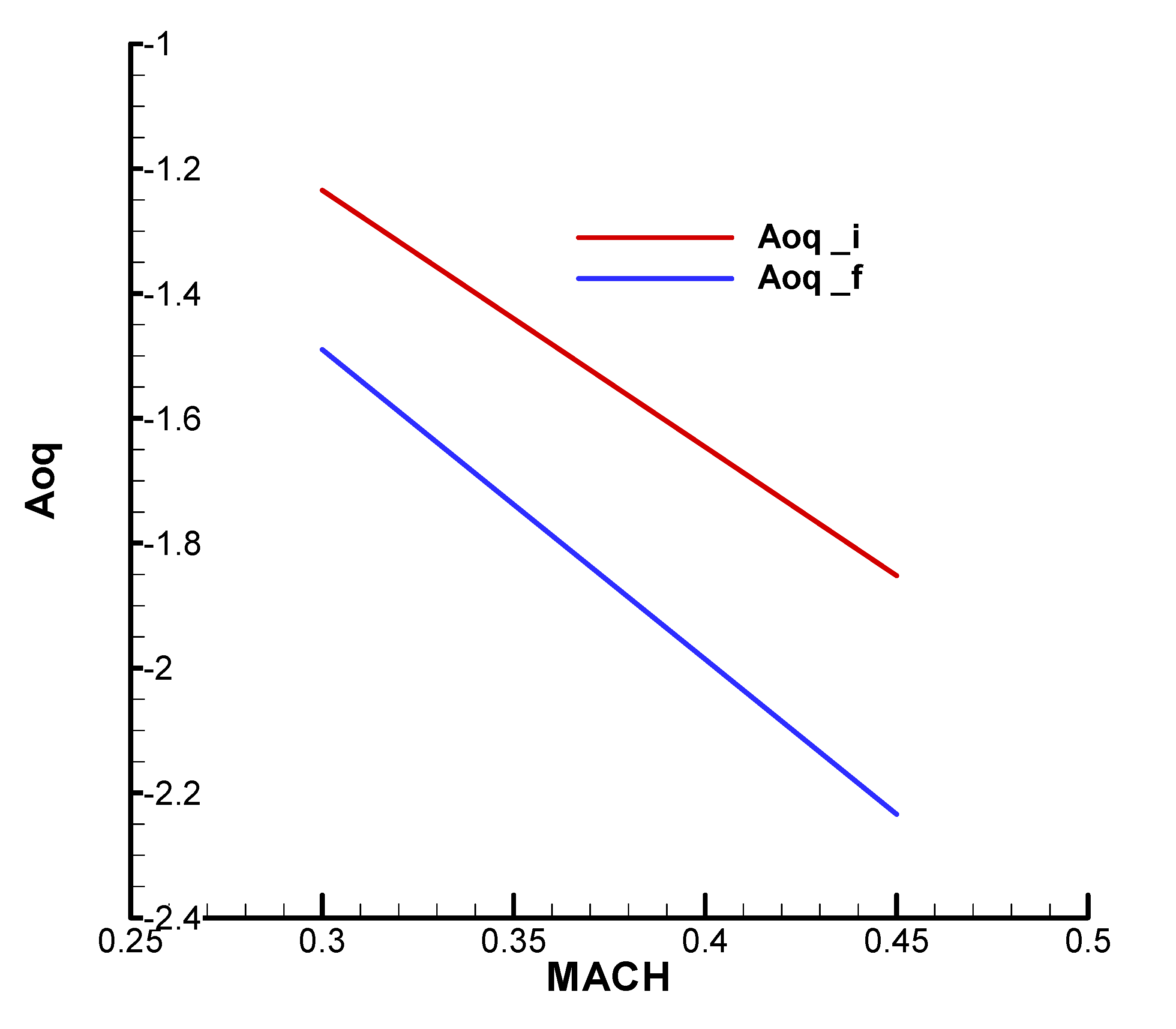
Figure B12.
Derivative term of the angeular velocity equation against unsteady incidence.
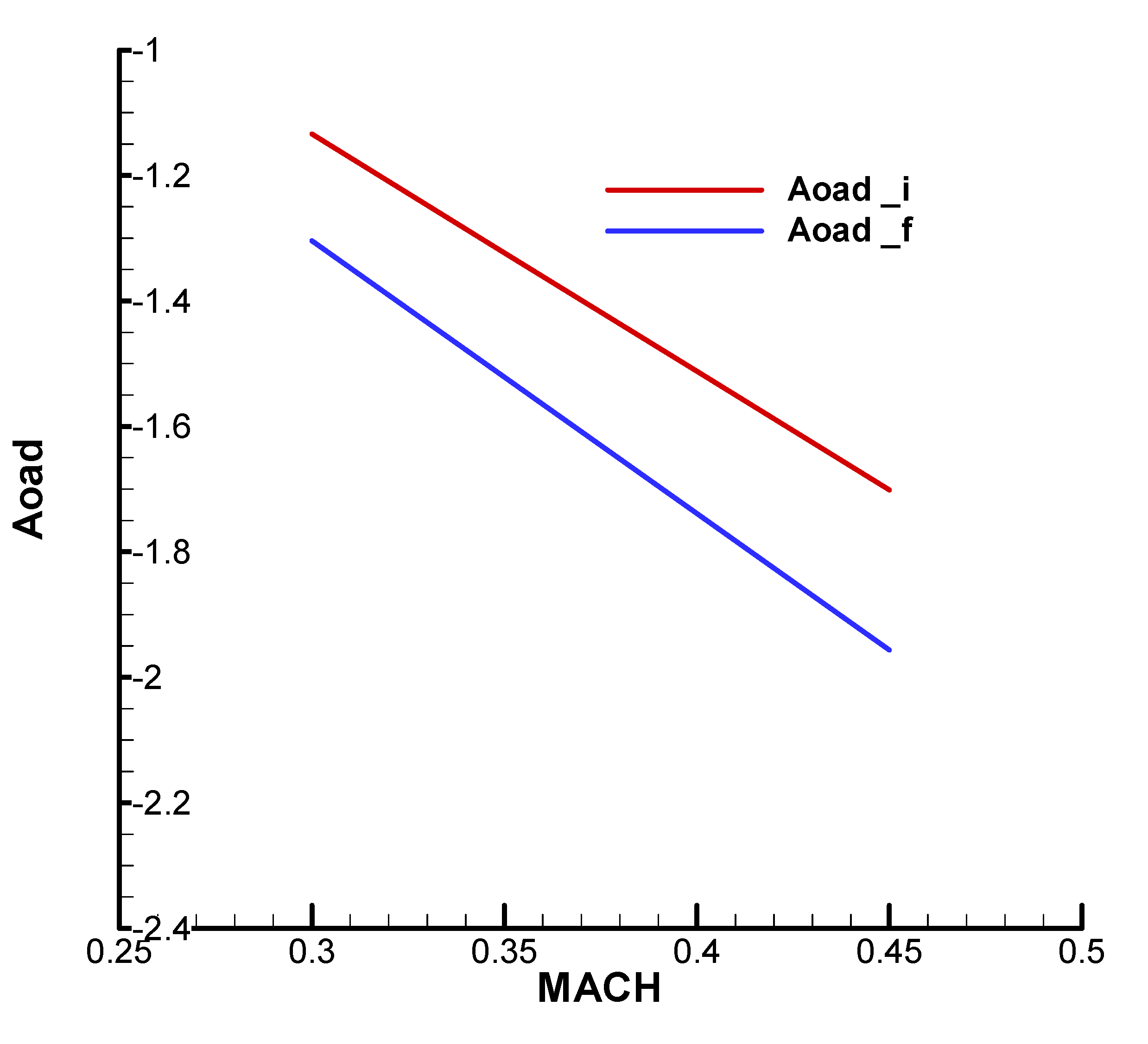
Figure B13.
Derivative term of the angular velocity equation against cross incidence – Magnus term.
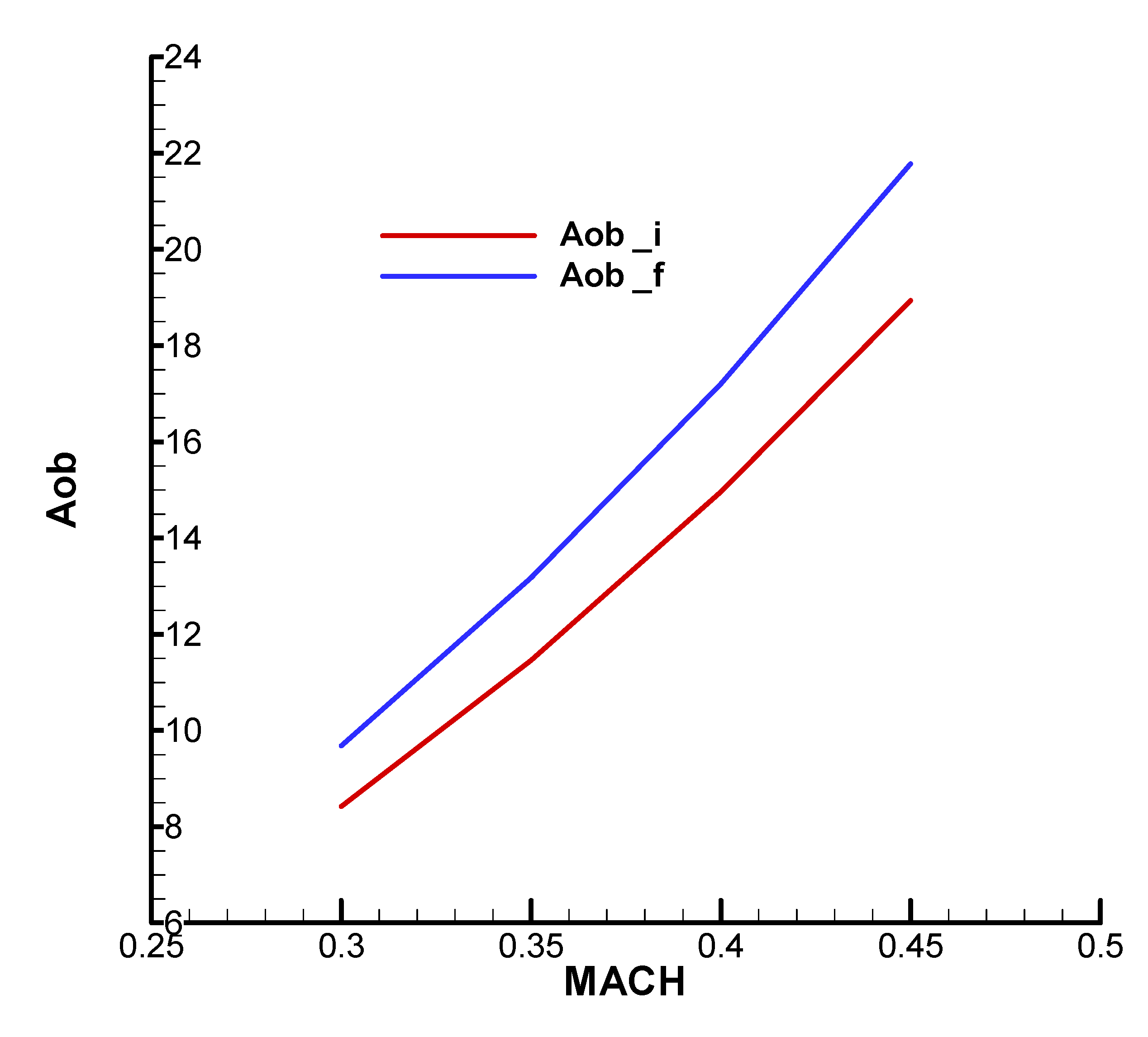
Figure B14.
Derivative term of the angular velocity equation against the cross angular velocity – Magnus and gyroscopic term.
Figure B14.
Derivative term of the angular velocity equation against the cross angular velocity – Magnus and gyroscopic term.
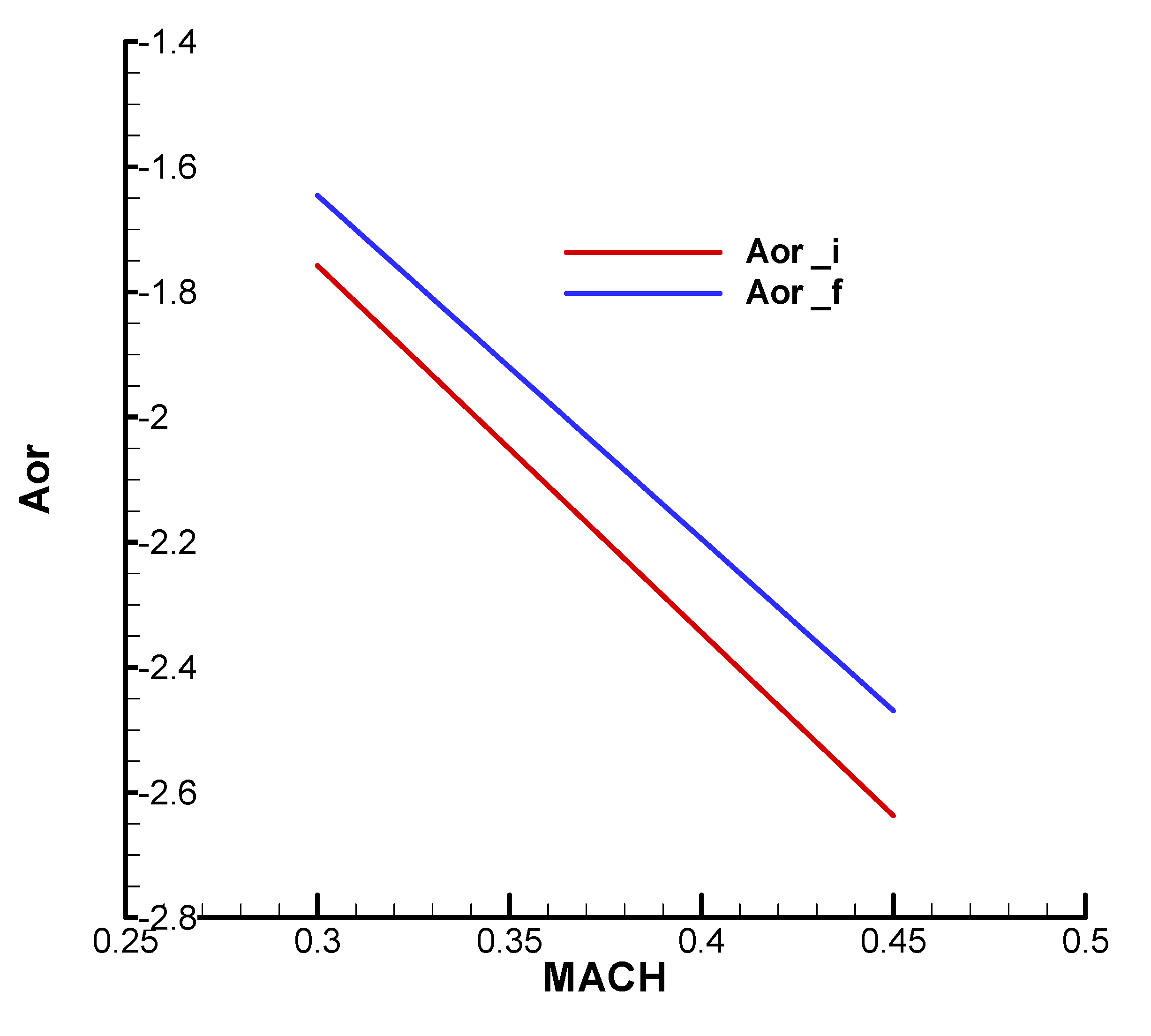
Command Matrix
Figure B15.
Derivative term of the incidence equation against thrust deflection.
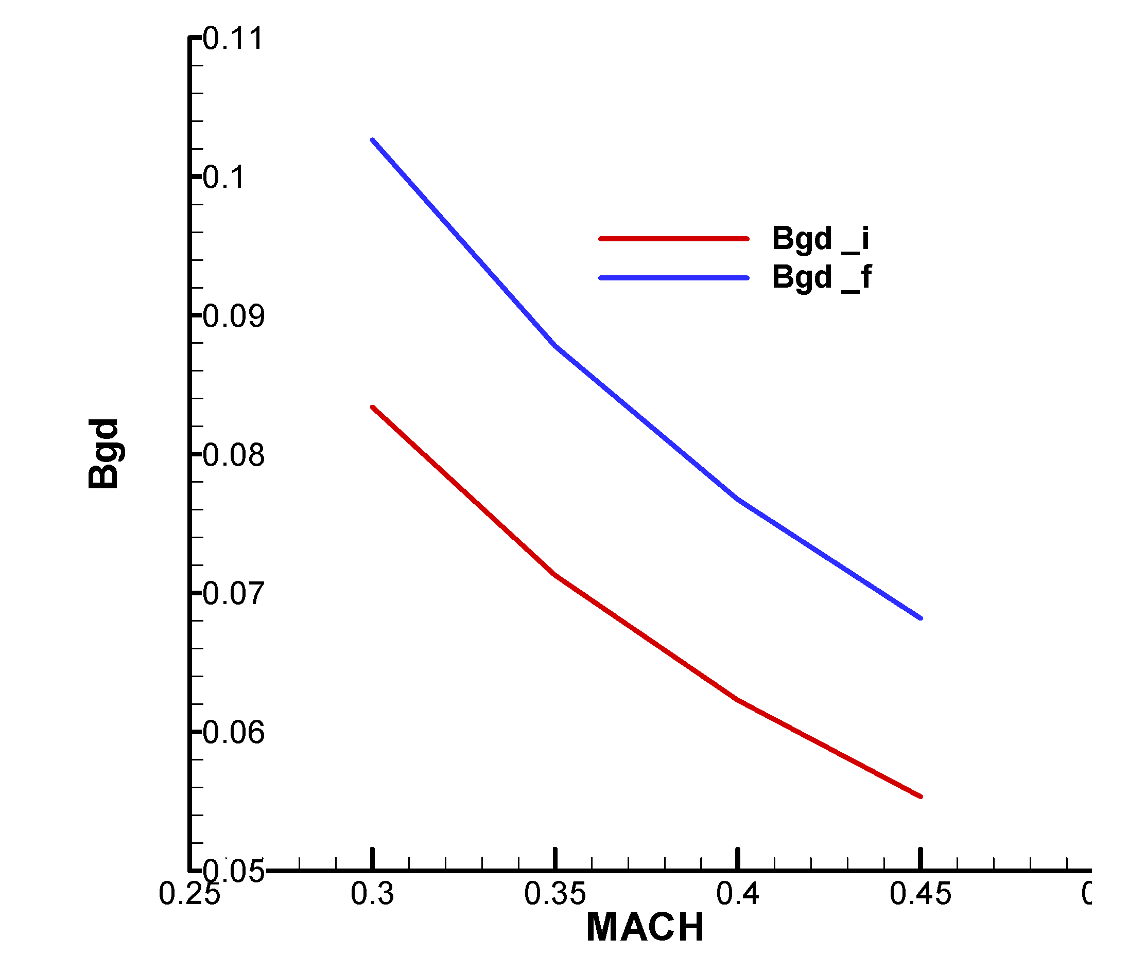
Figure B16.
Derivative term of the angular velocity equation against thrust deflection.
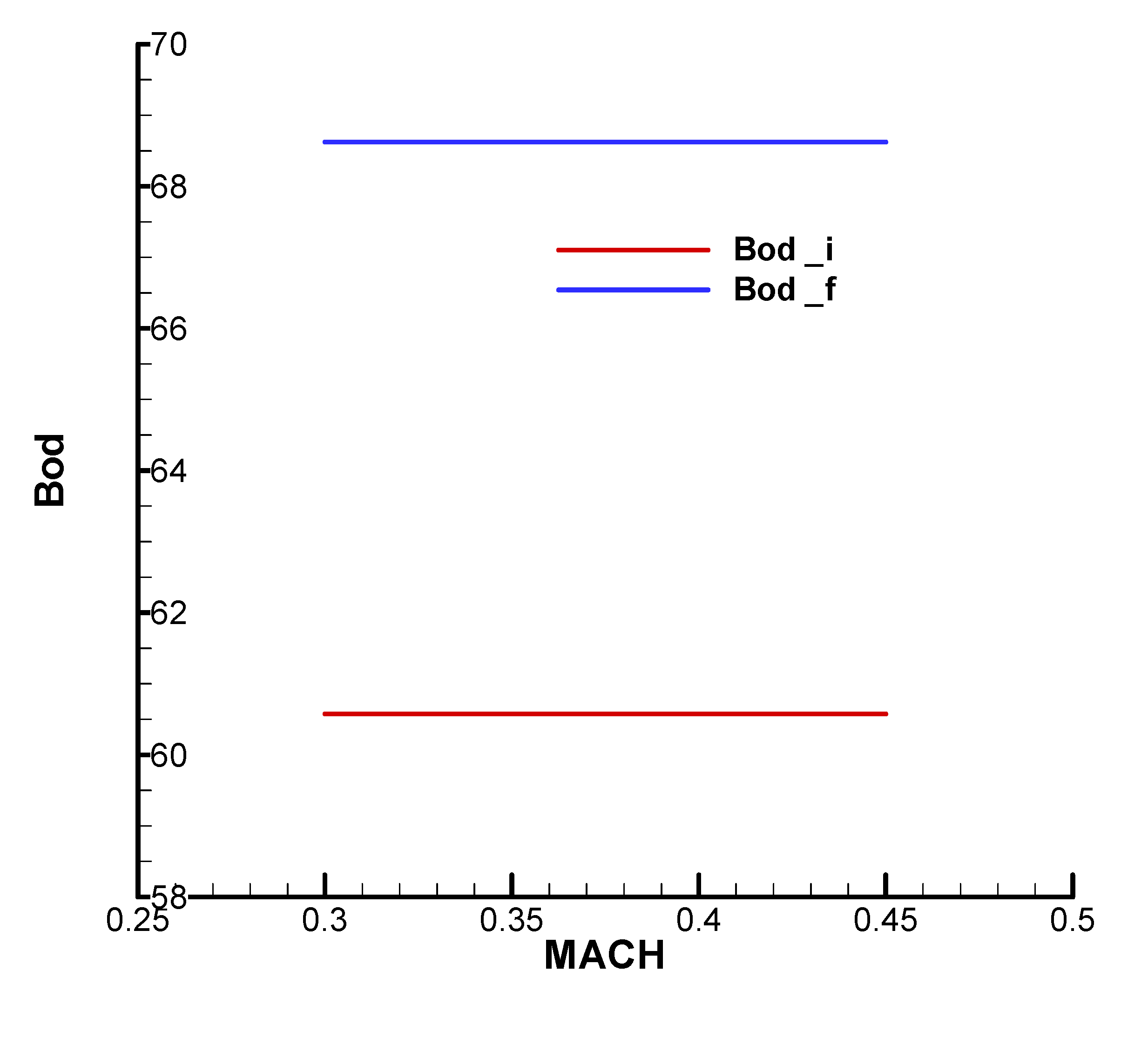
Flight Quality Parameters
Figure B17.
Static stability.
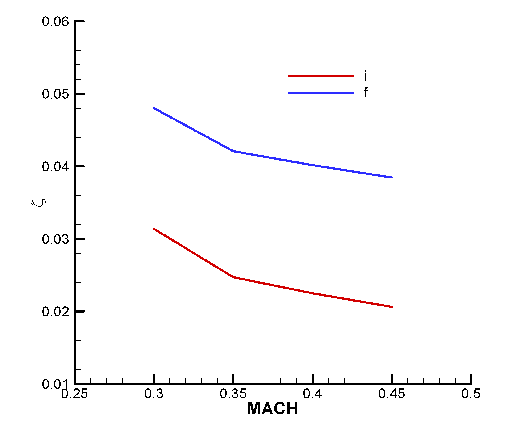
Figure B18.
Natural pulsation of nutation.
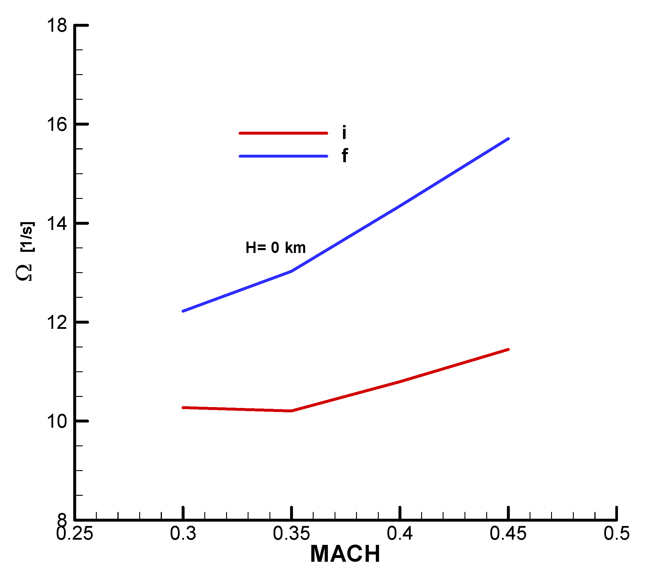
Figure B19.
Nutation damping factor.
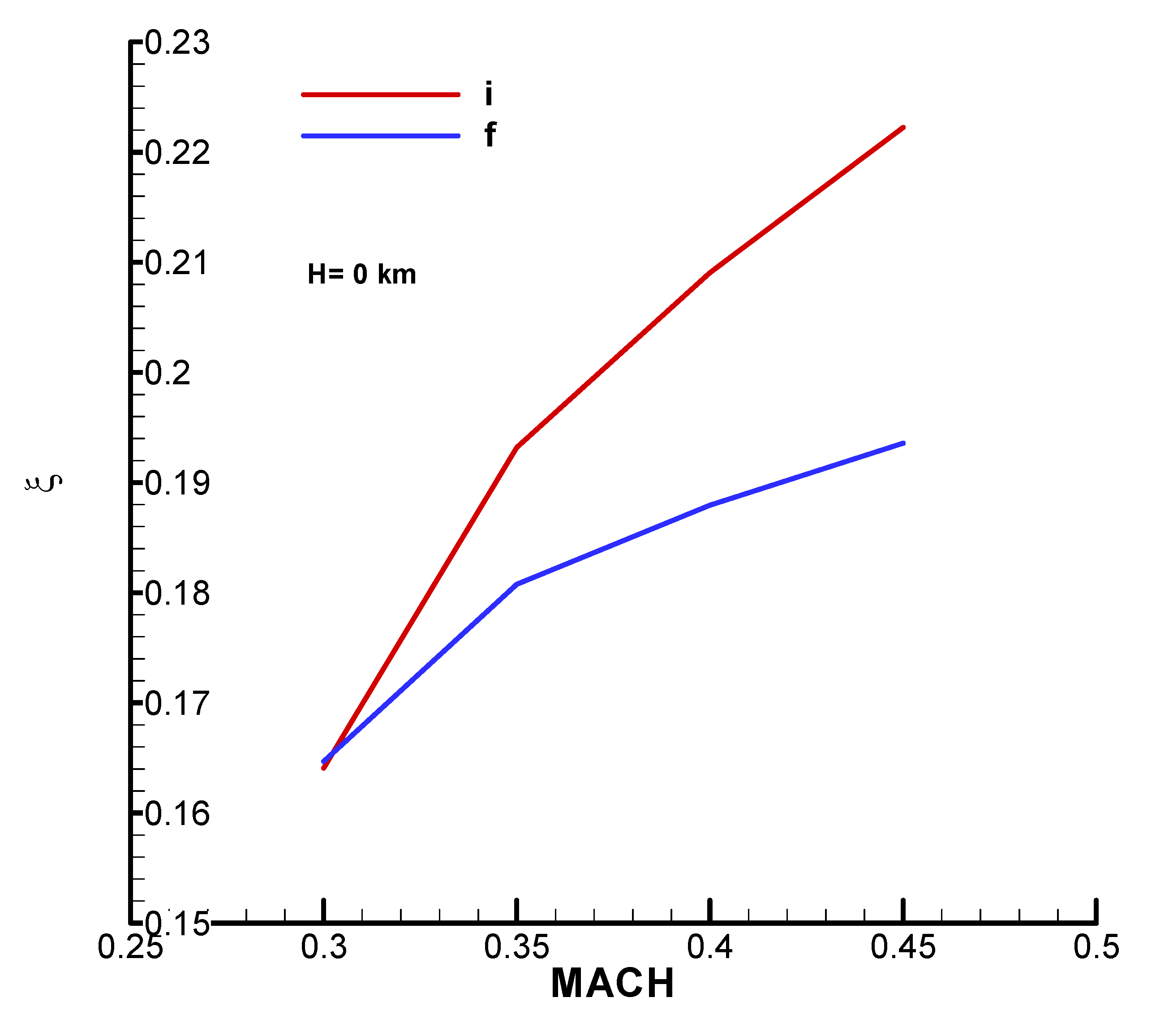
Figure B20.
Command factor.
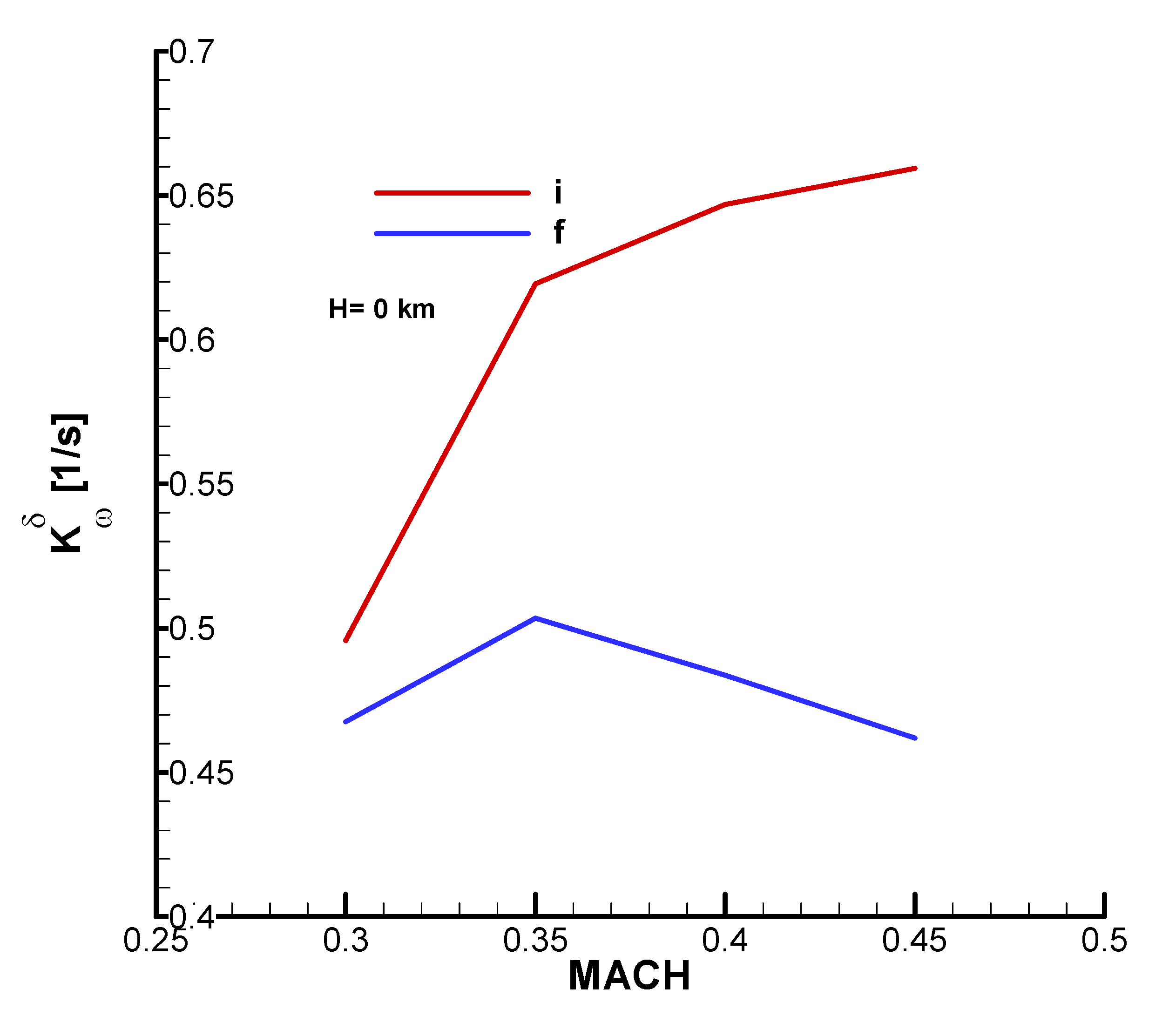
Figure B21.
The time constant of the missile.
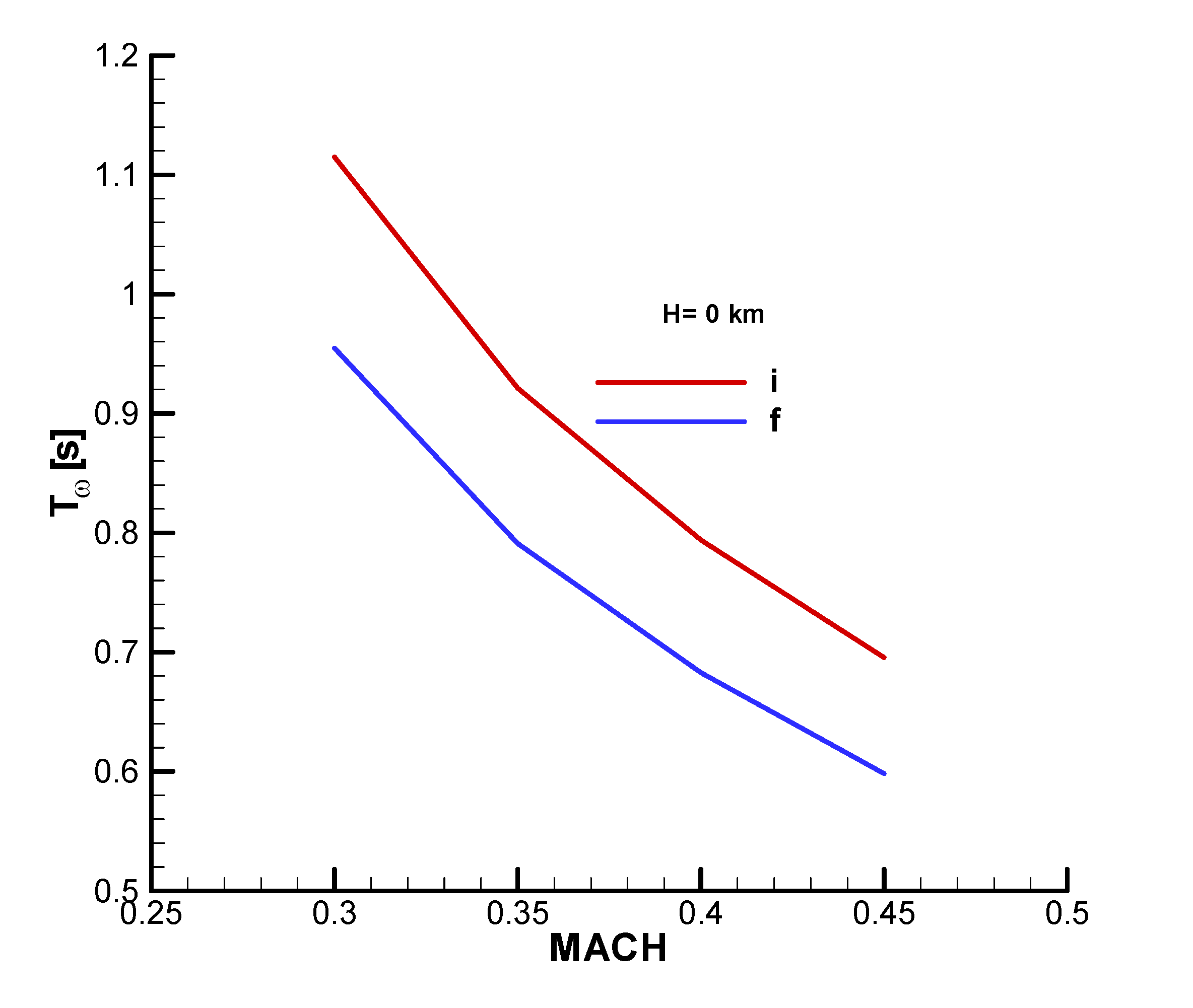
Figure B22.
Maximum overload factor.
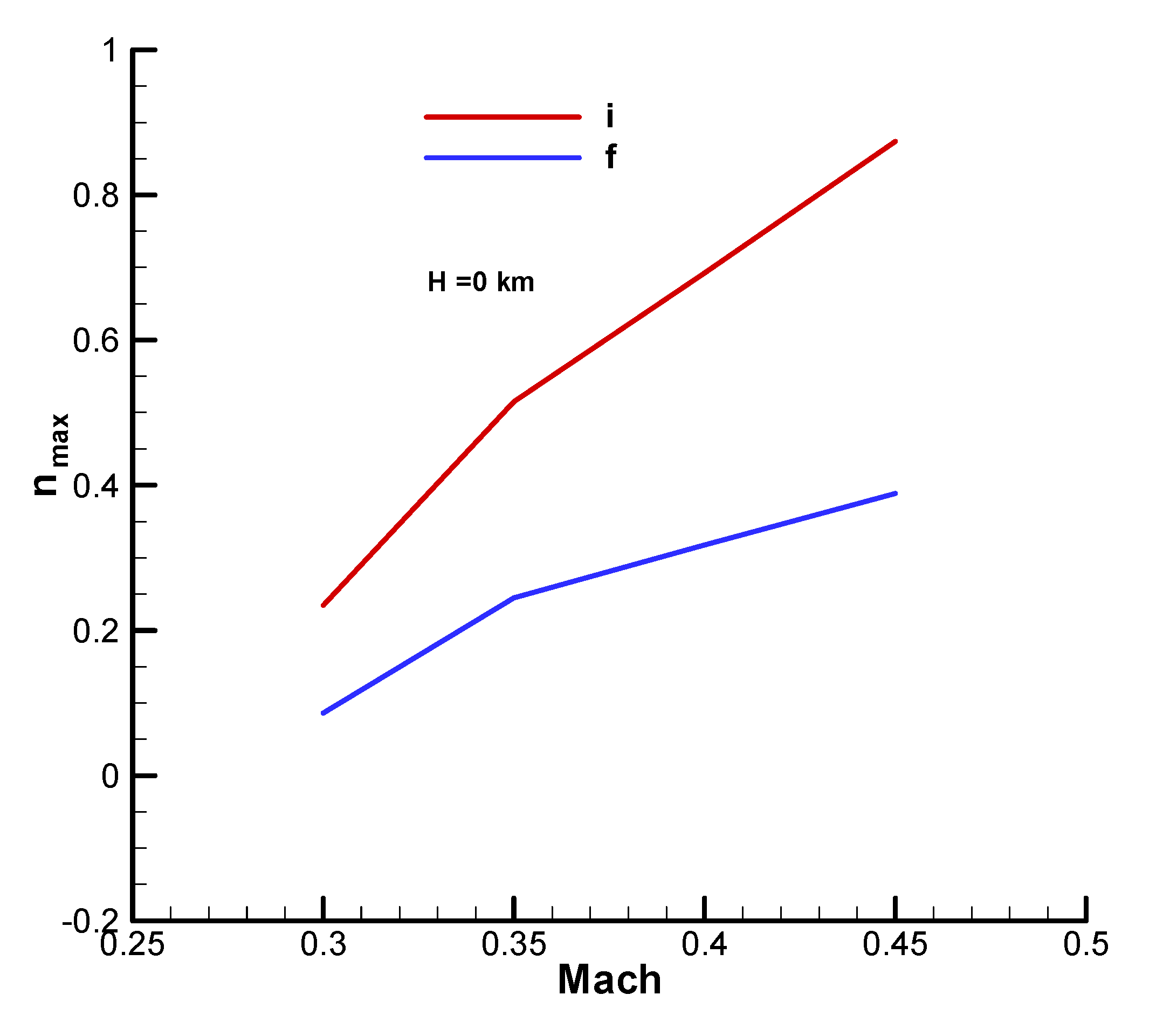
Appendix C. Frank-Wall Analyses Results
Coefficients of the Characteristic Polynomial
Figure C1.
Coefficient of the characteristic polynomial – the real part, initial; .
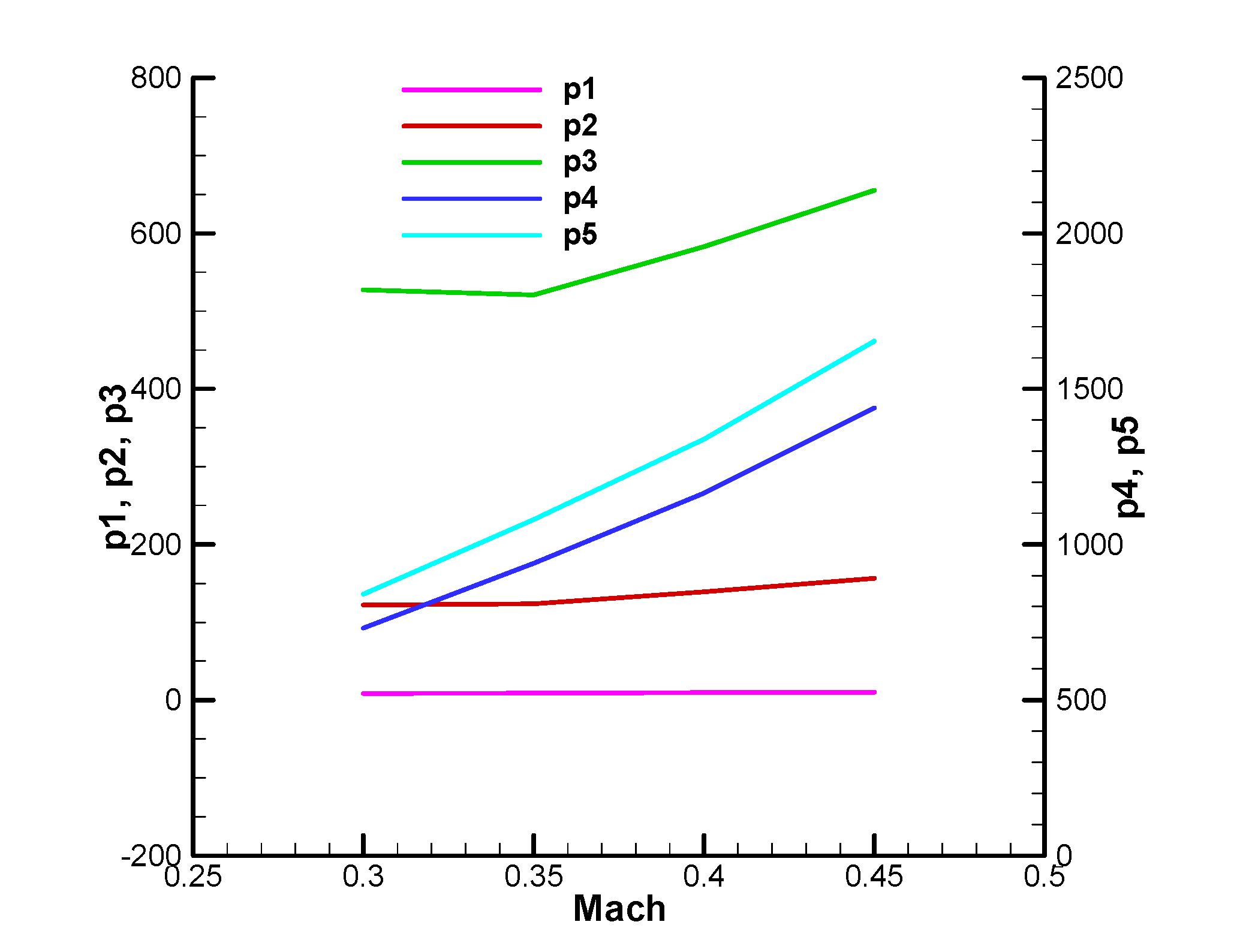
Figure C2.
Coefficient of the characteristic polynomial – the real part, initial; .
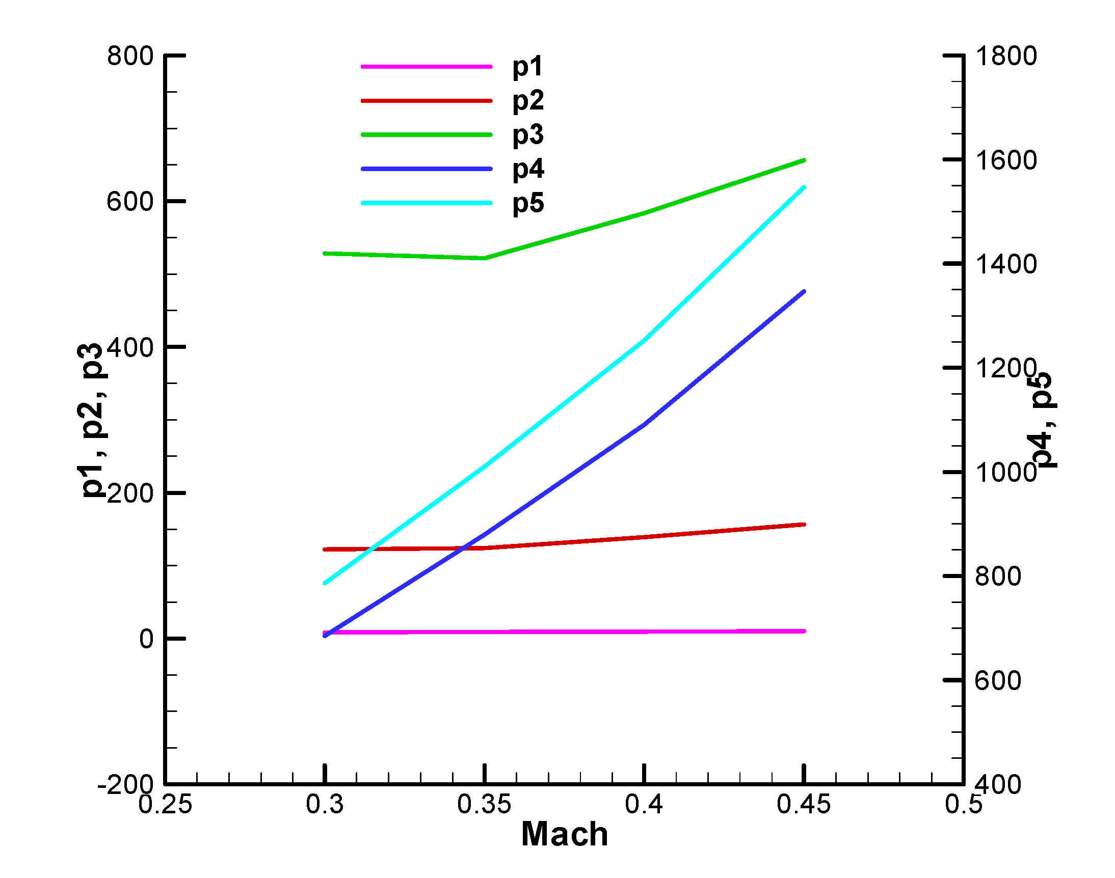
Figure C3.
Coefficient of the characteristic polynomial – the real part, final; .
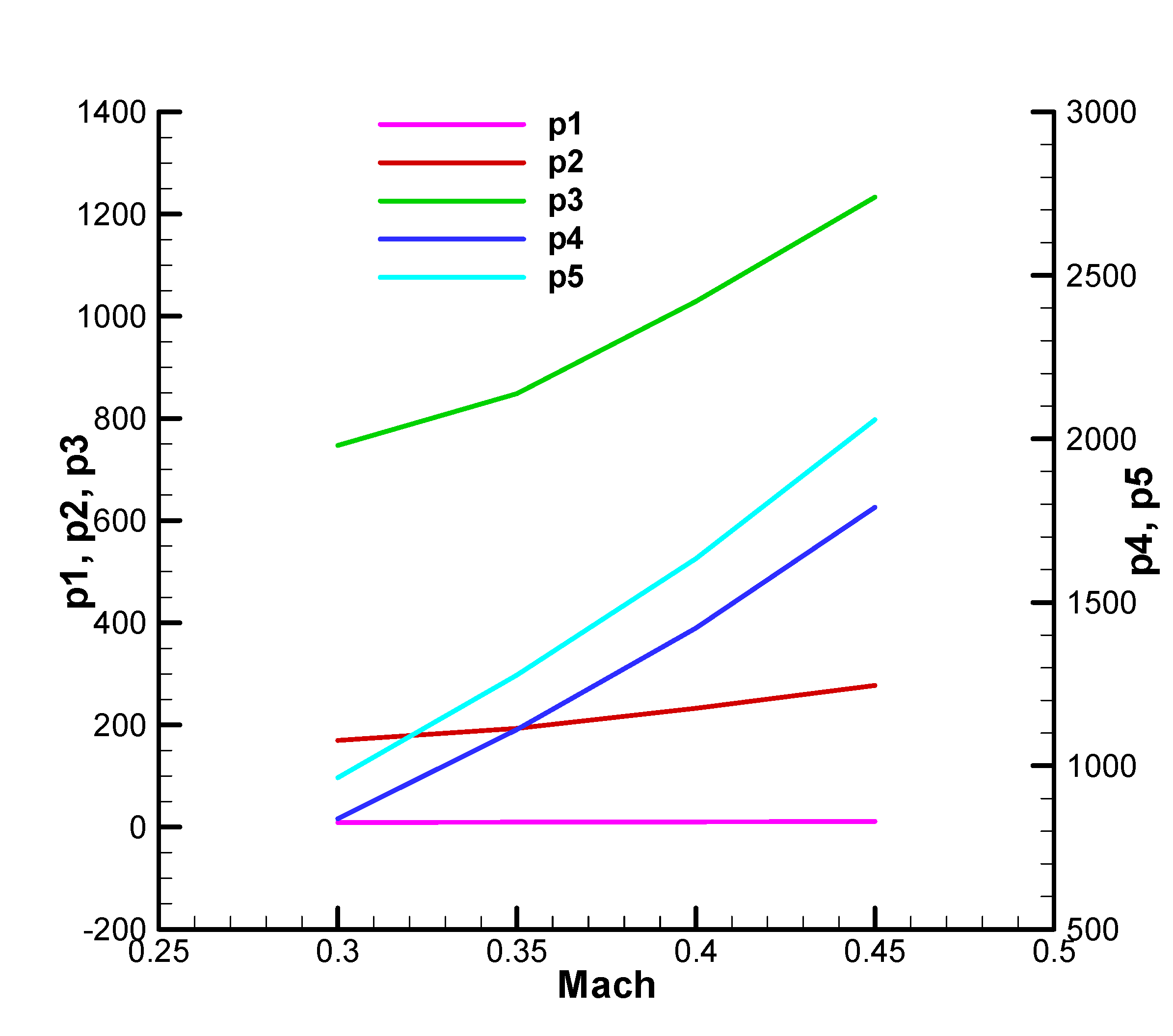
Figure C4.
Coefficient of the characteristic polynomial – the real part, final; .
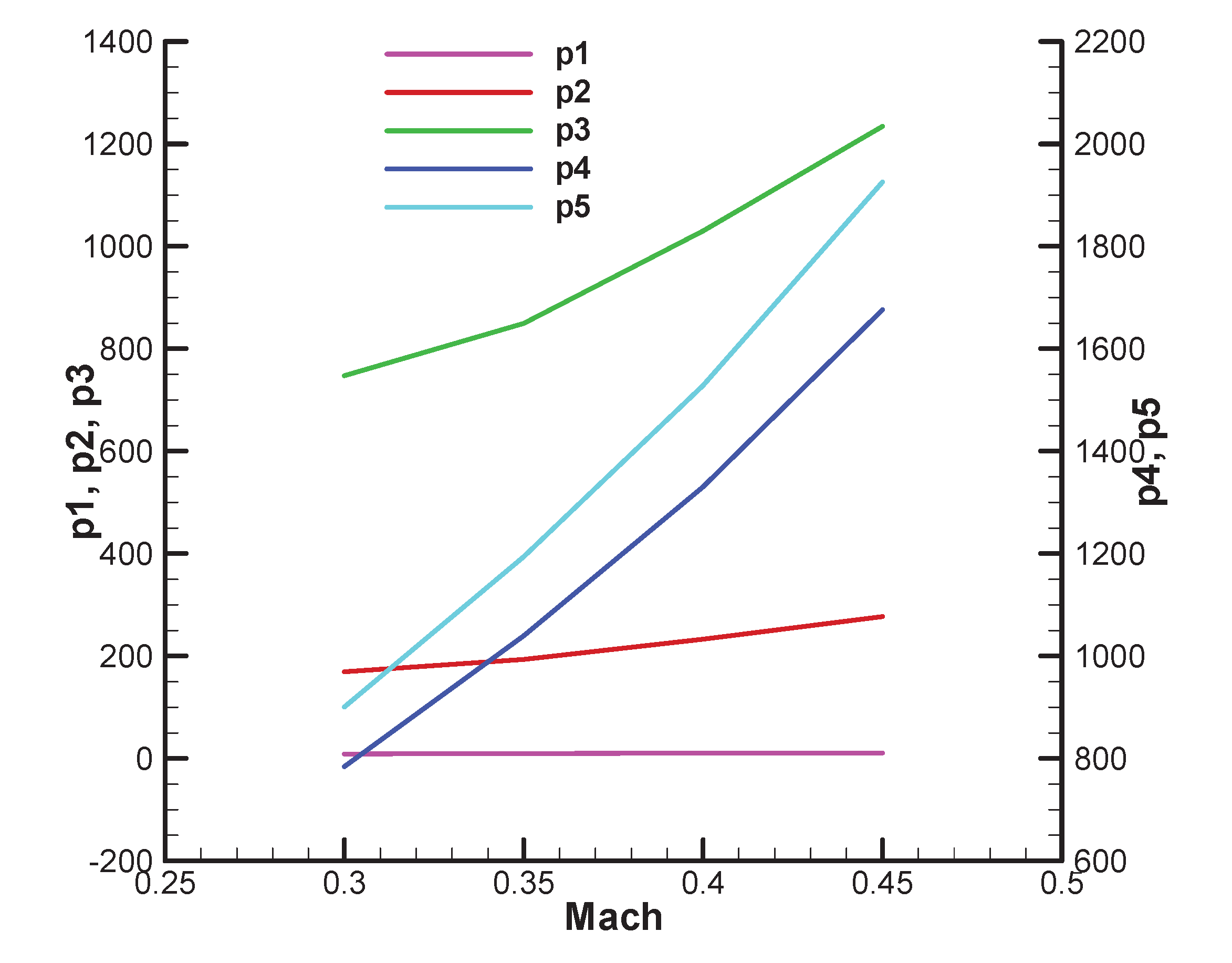
Figure C5.
Coefficient of the characteristic polynomial – the imaginary part, initial; .
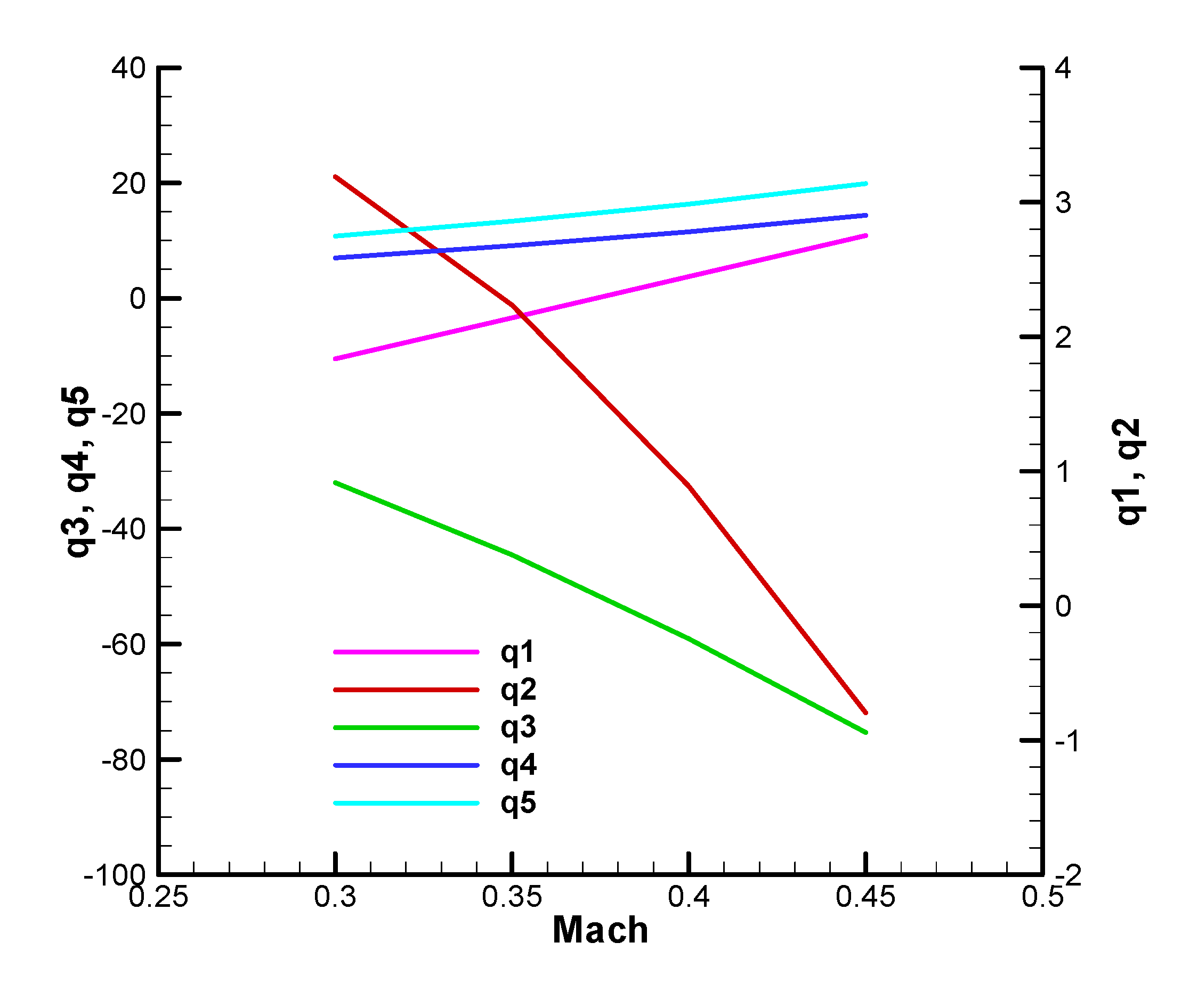
Figure C6.
Coefficient of the characteristic polynomial – the imaginary part, initial; .
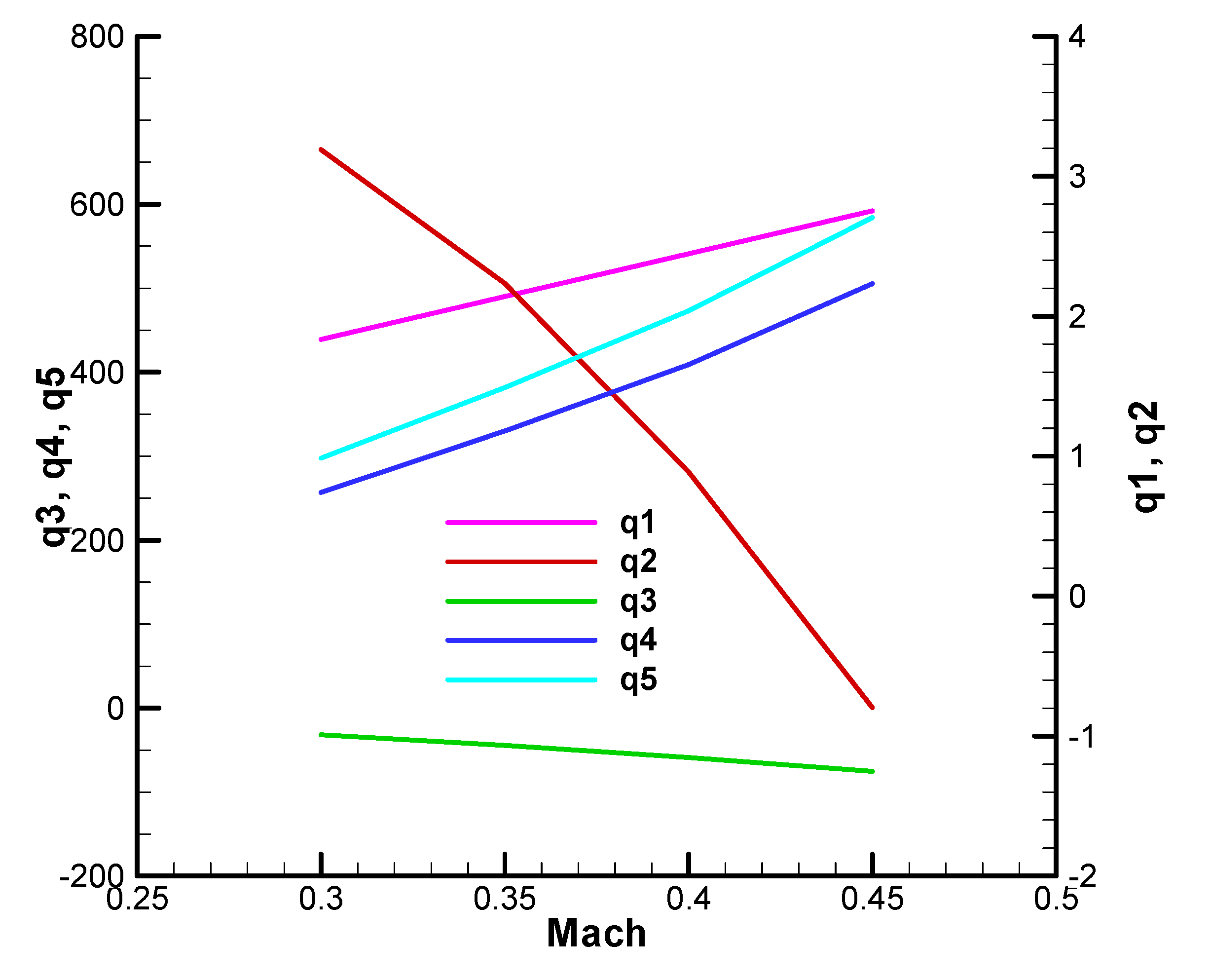
Figure C7.
Coefficient of the characteristic polynomial – the imaginary part, final; .
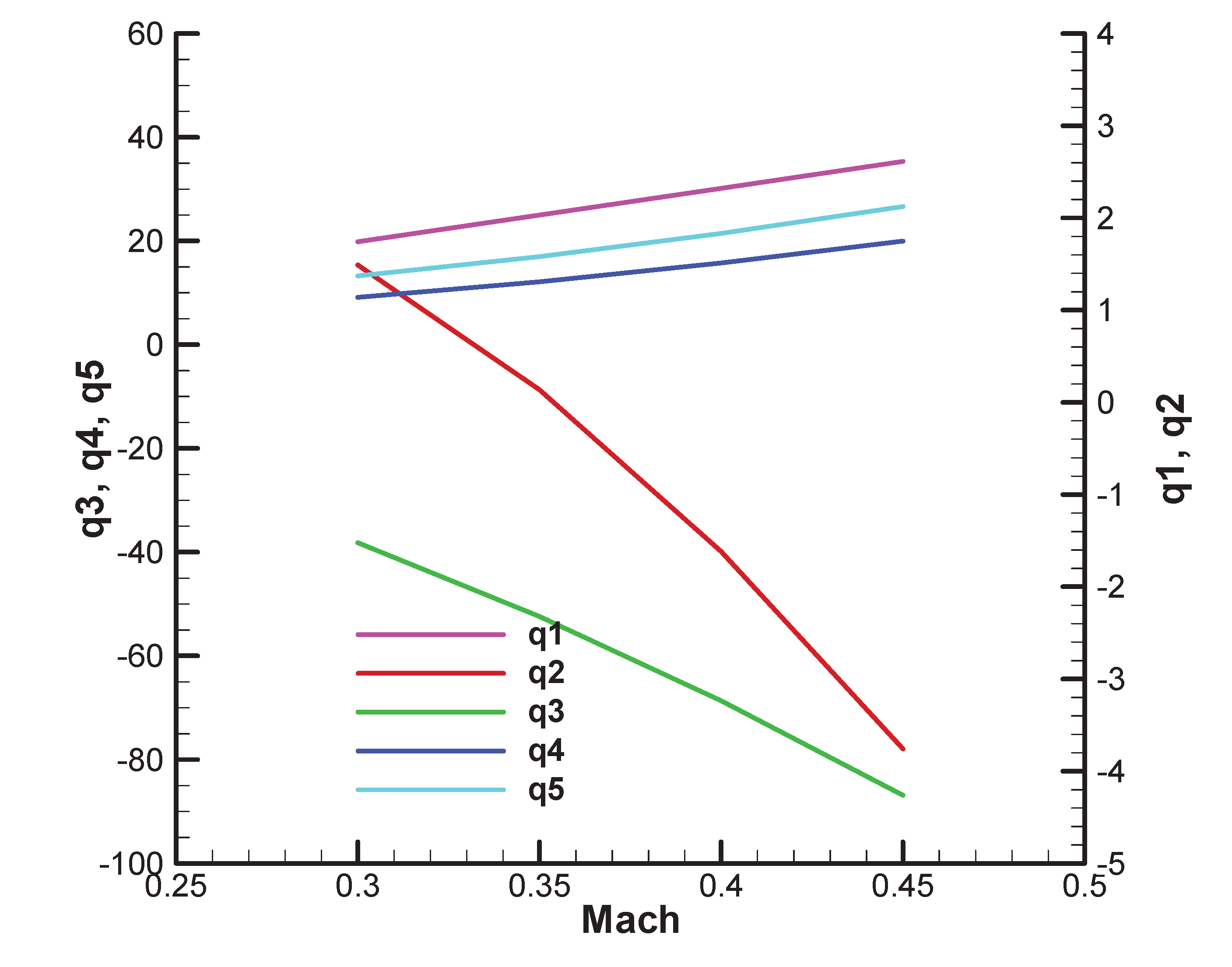
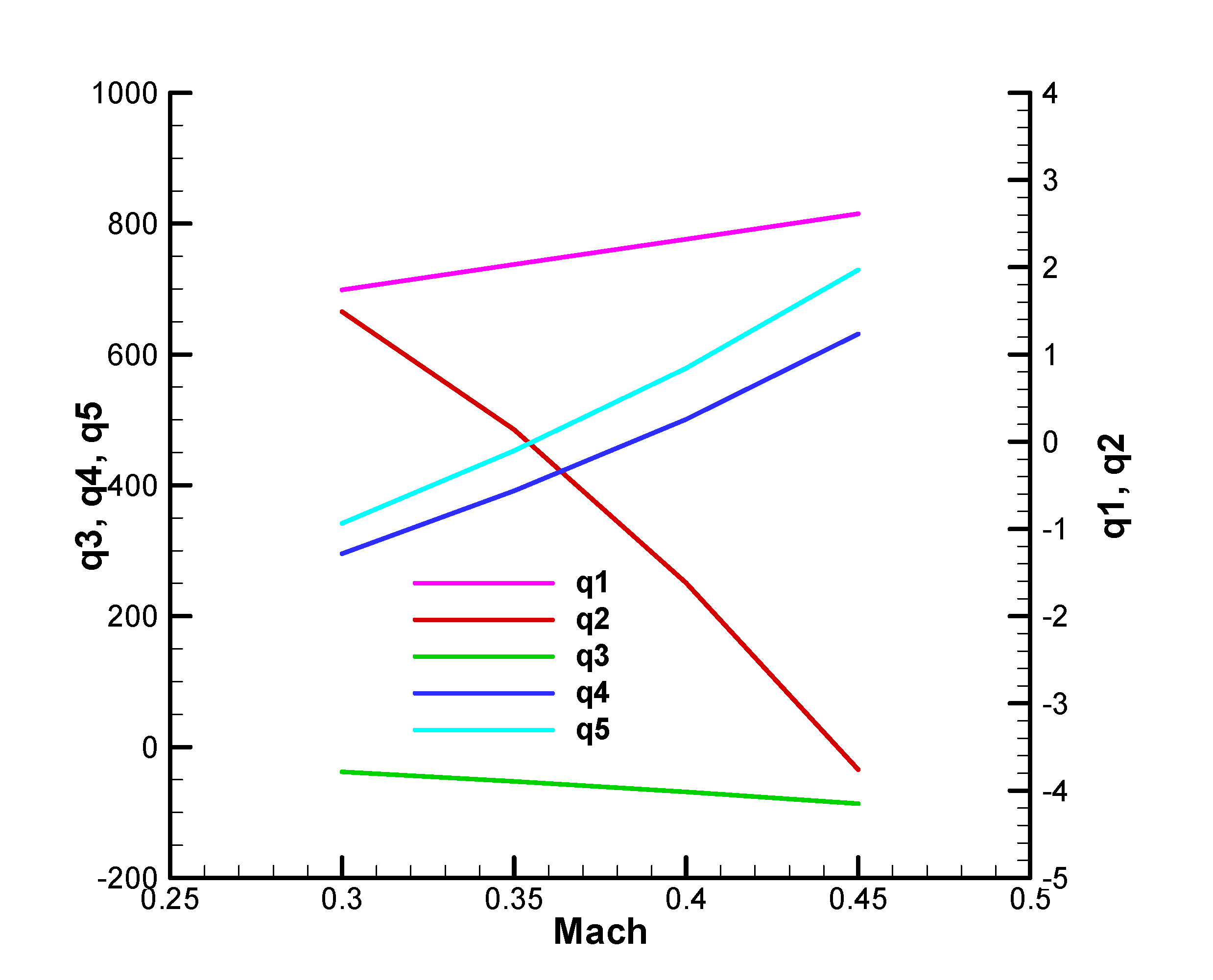
Figure C8.
Coefficient of the characteristic polynomial – the imaginary part, final; .
Stability Parameters F-W
Figure C9.
Stability parameters F-W – initial; .
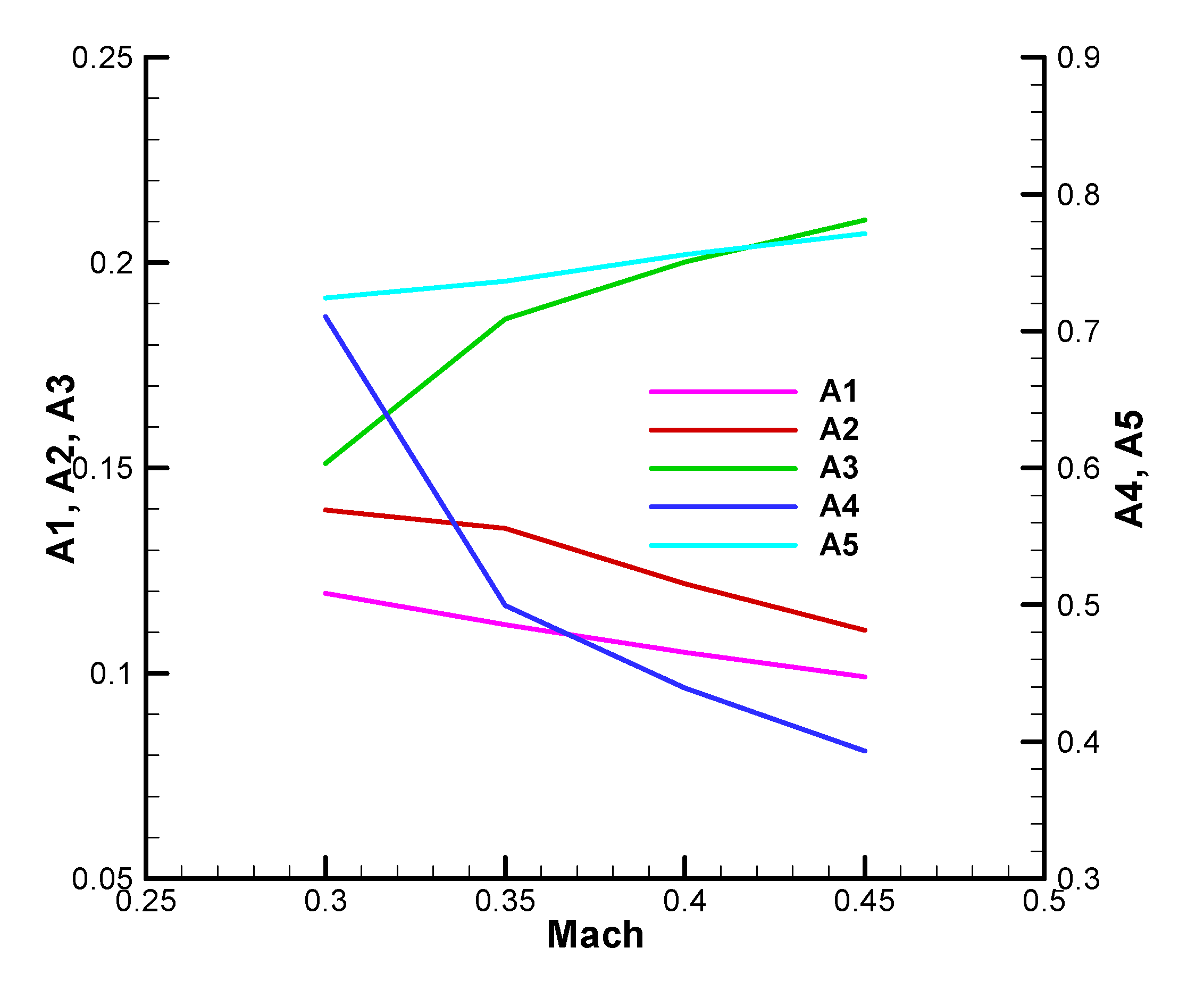
Figure C10.
Stability parameters F-W – initial; .
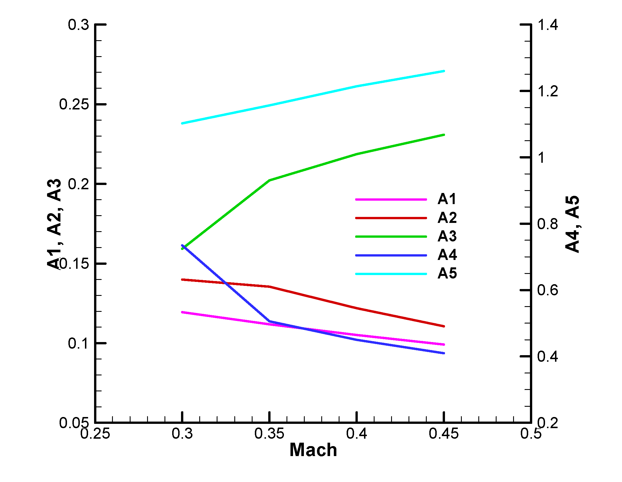
Figure C11.
Stability parameters F-W – final; .
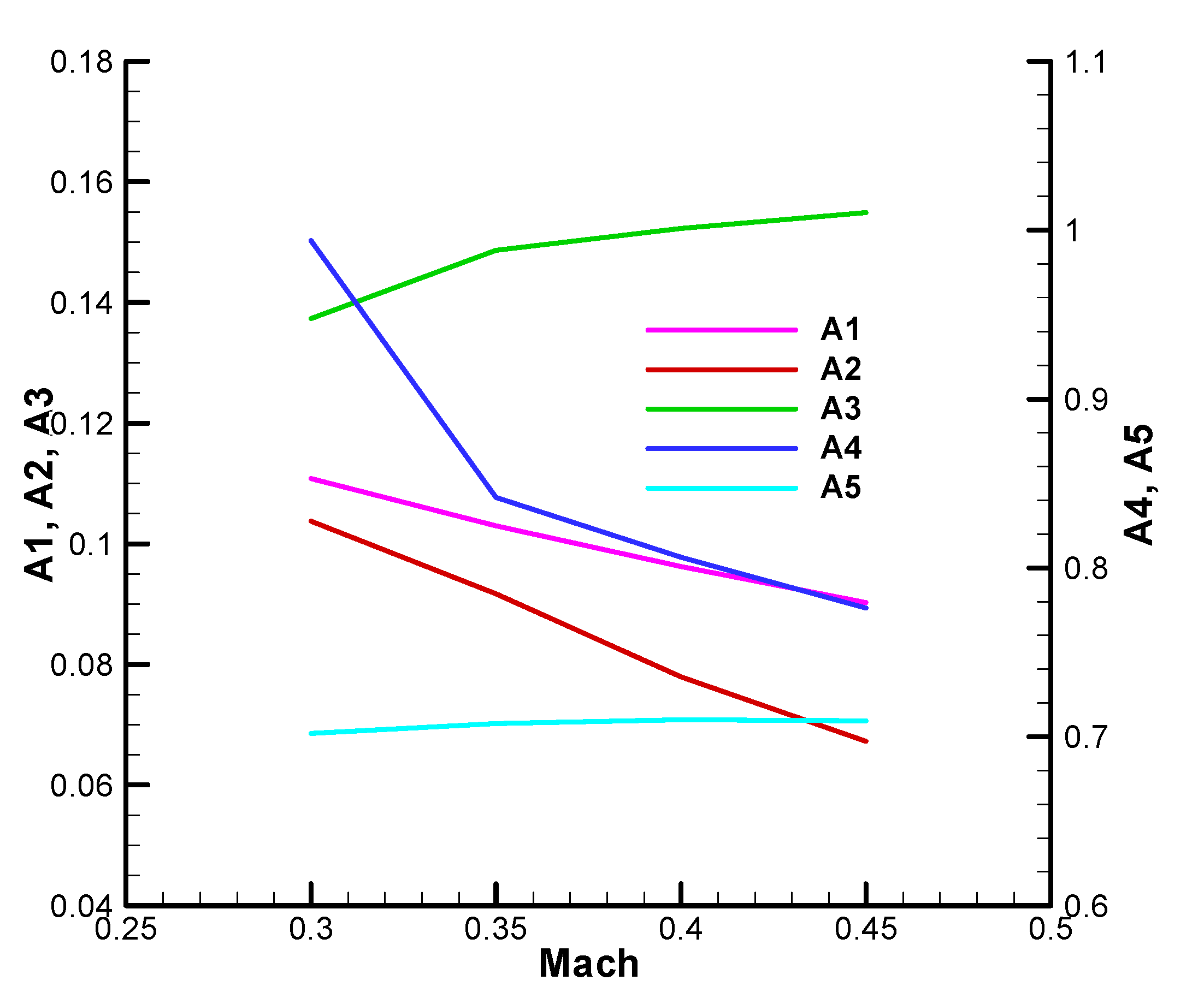
Figure C12.
Stability parameters F-W – final; .
Appendix D. The Root Locus of the Characteristic Polynomial
The diagrams are obtained for a range of Mach numbers: 0.3...0.45.
Characteristic Polynomial with Real Coefficients
Figure D1.
Roots of the characteristic polynomial with real coefficients – initial.
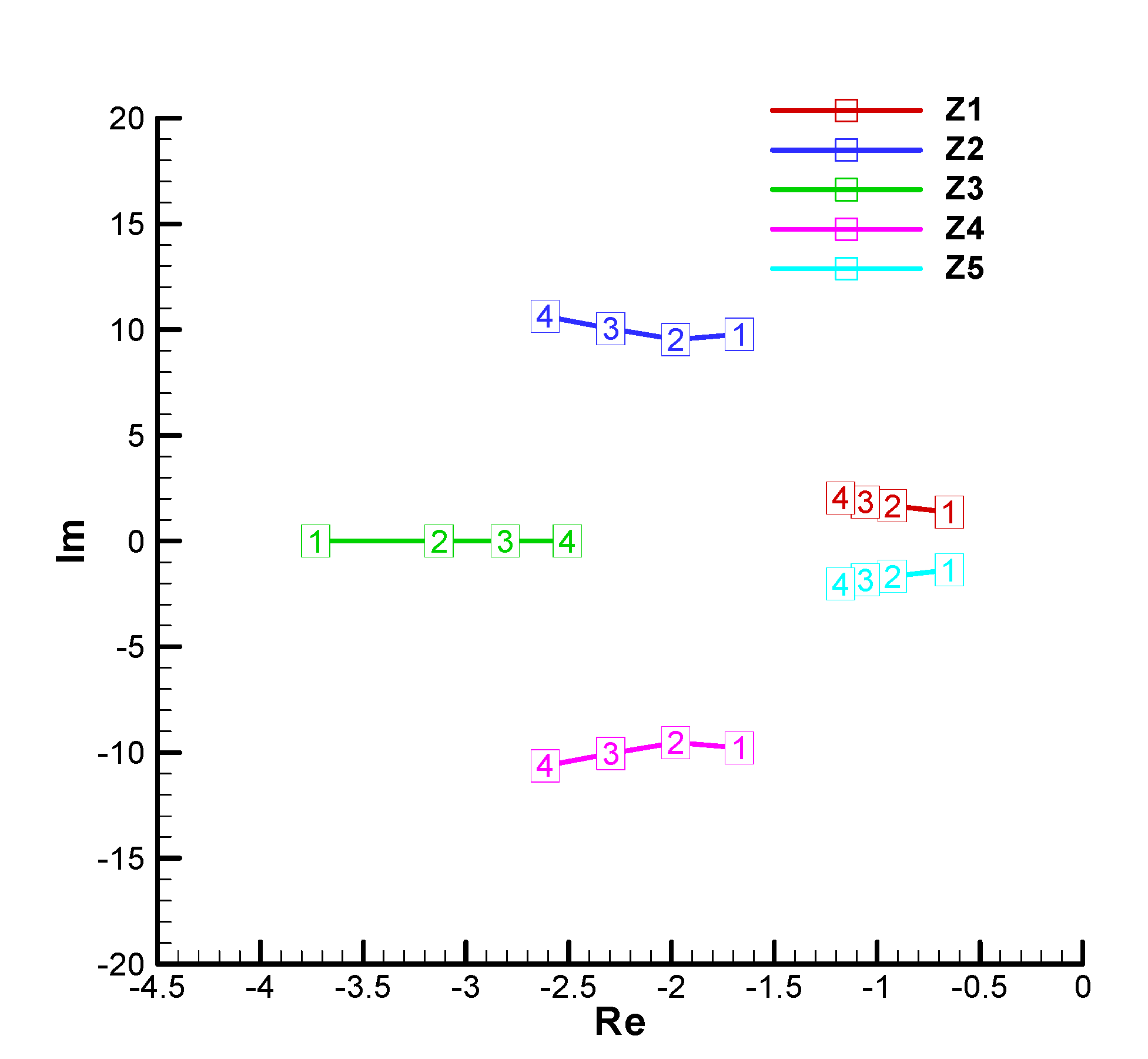
Figure D2.
Roots of the characteristic polynomial with real coefficients – final.
Characteristic Polynomial with Complex Coefficients
Figure D3.
Roots of the characteristic polynomial with complex coefficients– initial; .
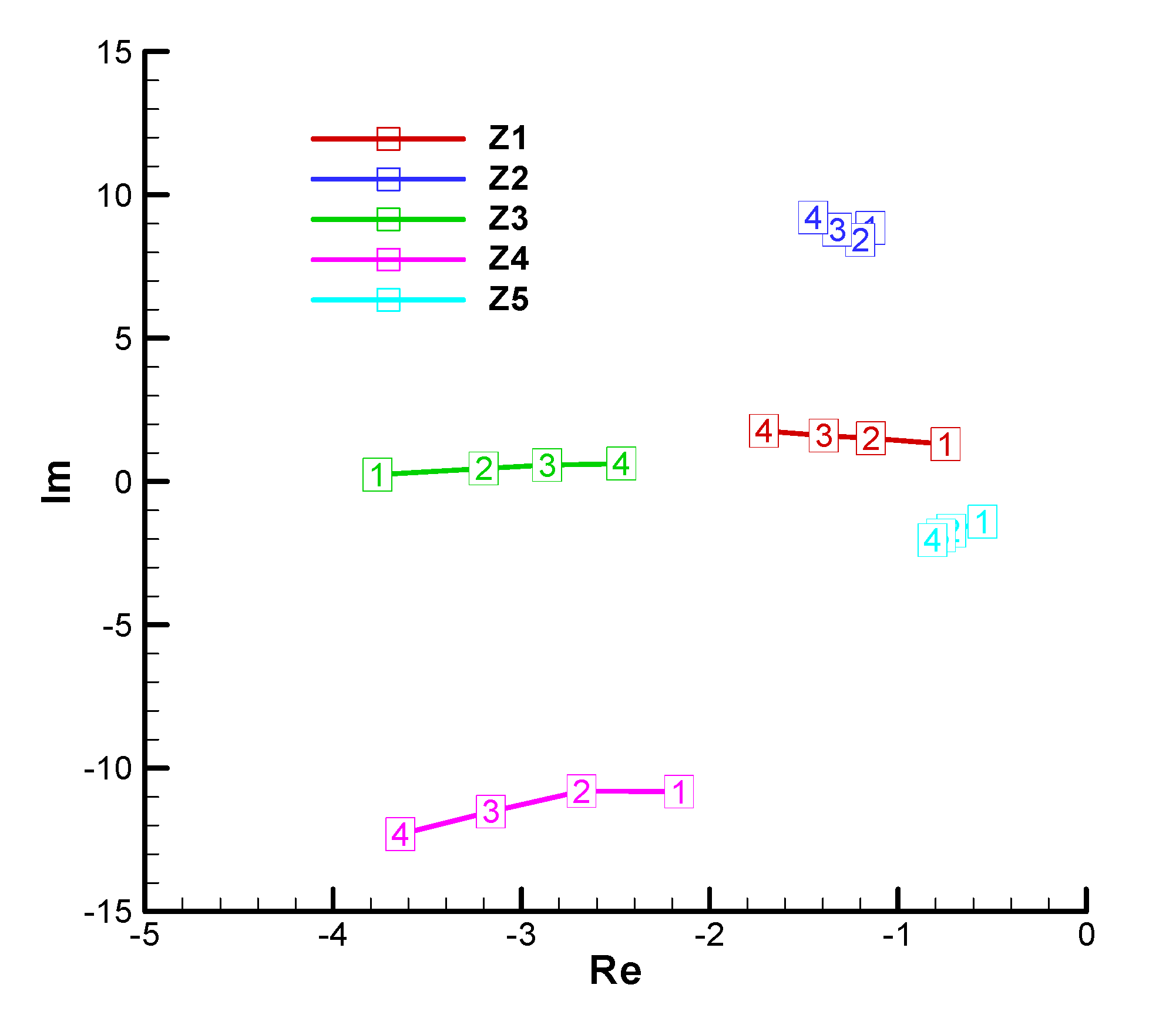
Figure D4.
Roots of the characteristic polynomial with complex coefficients– initial; .
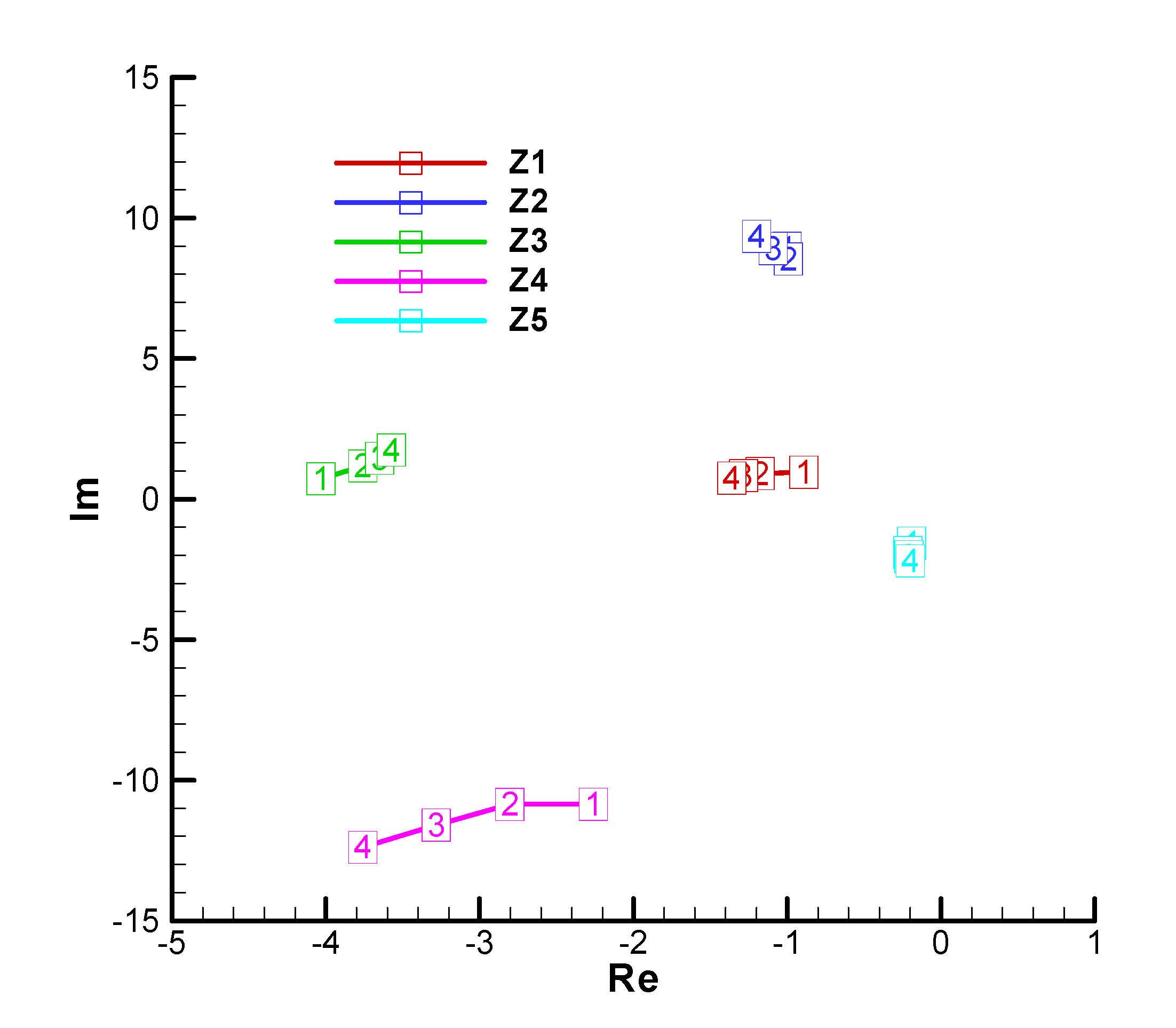
Figure D5.
Roots of the characteristic polynomial with complex coefficients – final; .
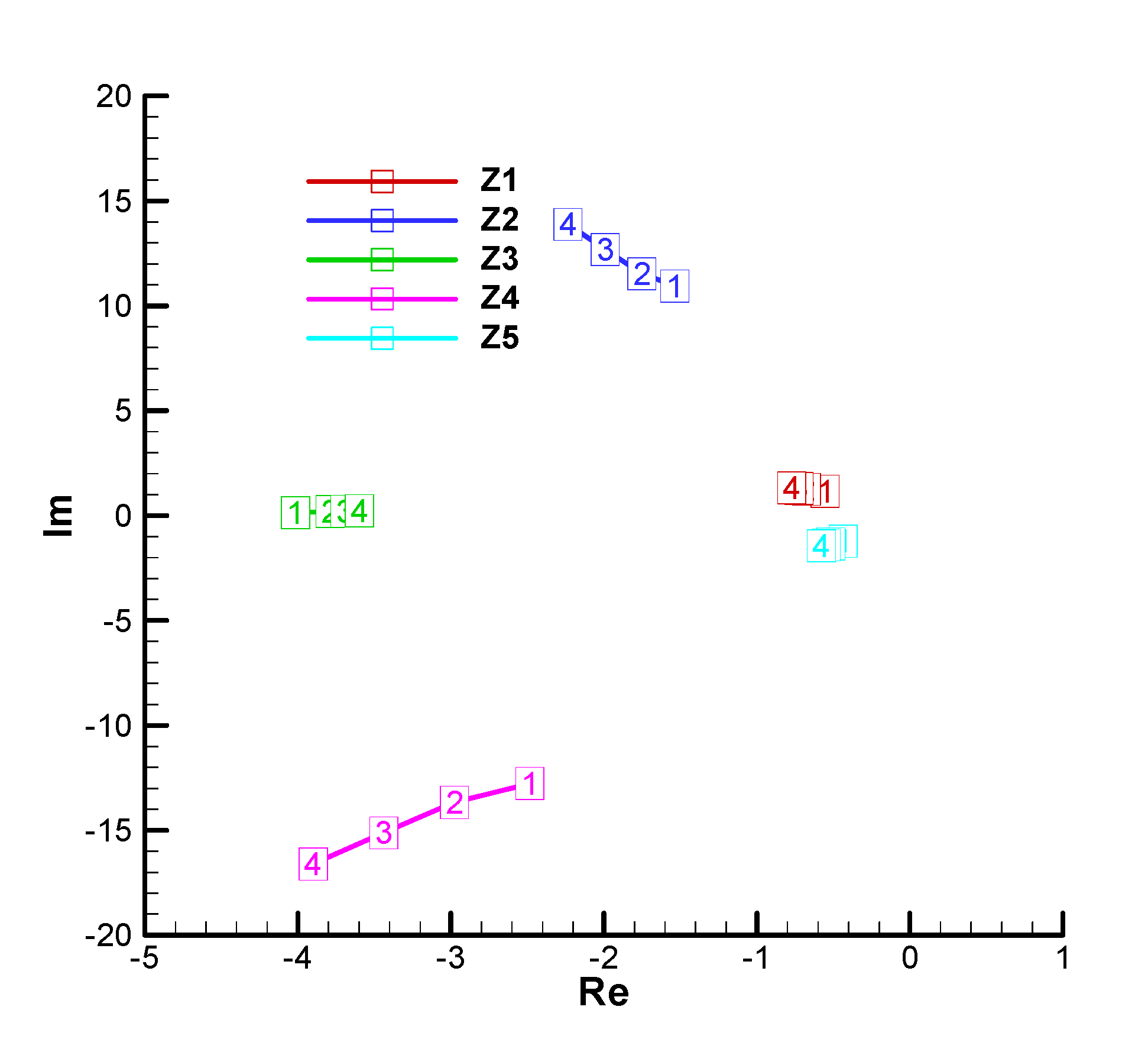
Figure D6.
Roots of the characteristic polynomial with complex coefficients – final;

Appendix E. Frank-Wall Stability Criterion for the 5th Order Polynomial
Considering a 5th order polynomial with complex coefficients:
to check if the real part of the roots is negative, first an associated polynomial is constructed:
after which, the ratio of the polynomials is put in the form:
According to the F-W stability theory [19], the necessary and sufficient condition for all roots of the polynomial (E1) to have the negative real part is that that and that be pure complex numbers or null.
In the same paper [19], the algorithm for calculating the F-W stability parameters is presented, which we detail below for a 5th order polynomial.
After which, for the 5th order polynomial is obtained successively:
Based on these relations, the stability parameters can be determined:
respectively:
Check for non-rolling case
For the case without rotation, the five parameters become:
where are the R-H determinants for the 5th order polynomial with real coefficients. It is observed that in this case the two conditions are equivalent:
References
- xxx. https://en.wikipedia.org/wiki/9M14_Malyutka. [Online].
- xxx, “https://en.wikipedia.org/wiki/MILAN,” [Online].
- xxx, “https://en.wikipedia.org/wiki/BGM-71_TOW,” [Online].
- Hu, X and Yang, SX. Coning motion instability of spinning missiles induced by the delay of strap-down seeker. CHINESE JOURNAL OF AERONAUTICS 2021, 33, 3360–3368. [Google Scholar]
- Hu, Shaoyong; Wang, Jiang; Wang, Yuchen; Tian, Song. Stability Limits for the Velocity Orientation Autopilot of Rolling Missiles. IEEE ACCESS 2021, 9, 110940–110951. [Google Scholar] [CrossRef]
- Zheng, Qiushi; Zhou, Zhiming, “Flight Stability of Canard-Guided Dual-Spin Projectiles with Angular Rate Loops,” INTERNATIONAL JOURNAL OF AEROSPACE ENGINEERING, 2020.
- Suiçmez, E.C.; Kutay, A.T. . Single channel digital controller design for a high spinning rate rolling airframe missile. AERONAUTICAL JOURNAL 2022, 126, 1815–1833. [Google Scholar] [CrossRef]
- J. Karimi. A new closed form solution for dynamic stability analysis of rolling airframes having one pair on-off actuator. Aviation, Open Access 2021, 25, 92–103. [Google Scholar]
- Botez, RM; Chelaru, V; Parvu, P; Gheorghe, C. . Calculus model for a rolling guided missile. JOURNAL OF VIBRATION AND CONTROL 2001, 7, 863–889. [Google Scholar] [CrossRef]
- Chelaru, T.-V. , Constantinescu, C. In E.. Theoretical and experimental solutions for multistage quasi-guided rocket.. in Proceedings of the International Astronautical Congress, IAC, Washington; 2019. [Google Scholar]
- Chelaru, T. V, Constantinescu C.E., Pana, V., Ene, C., Chelaru A. Stability of single channel homing rolling aerospace vehicle. Aerospace 2024, 11, 60. [Google Scholar] [CrossRef]
- Zheng, Duo; Lin,Lin, Defu; Wang, Jiang; Xu, Xinghua. Dynamic stability of rolling missiles employing a two-loop autopilot with consideration for the radome aberration parasitic feedback loop. AEROSPACE SCIENCE AND TECHNOLOGY 2017, 61, 1–10. [Google Scholar] [CrossRef]
- Tian, Song; Lin, Defu; Wang, Jiang; Li, Bin. Dynamic stability of rolling missiles with angle-of-attack feedback three-loop autopilot considering parasitic effect. AEROSPACE SCIENCE AND, TECHNOLOGY 2017, 71, 592–602. [Google Scholar] [CrossRef]
- Zheng, Duo; Lin, Defu; Xu, Xinghua; Tian, Song. Dynamic stability of rolling missile with proportional navigation & PI autopilot considering parasitic radome loop. AEROSPACE SCIENCE AND TECHNOLOGY 2017, 67, 41–48. [Google Scholar]
- Qin, Sheng-jie; Zhang, Fu-xue. A Combination of Silicon Micro-gyroscope that Application Rotary Missile Attitude Control System. in 2011 INTERNATIONAL CONFERENCE ON PHYSICS SCIENCE AND TECHNOLOGY (ICPST), Hong Kong,, 2011.
- Yan, Xiaolong; Chen, Guoguang; Tian, Xiaoli. Two-Step Adaptive Augmented Unscented Kalman Filter for Roll Angles of Spinning Missiles Based on Magnetometer Measurements. MEASUREMENT & CONTROL. 2018, 51, 73–82. [Google Scholar]
- Jahangir,E. and Howe, R. M. Time-Optimal Attitude Control Scheme for a Spinning Missile. JOURNAL OF GUIDANCE, CONTROL, AND DYNAMICS 1993, 16, Narch–April. [Google Scholar]
- Kocetkov,V.T, Polovko,A.M., Ponomarev, B.M.,Theory of self-guided and remote-controlled missile systems, Moskva: Nauka, 1964.
- E. Frank. On the zeros of polynomials with complex coefficients. Bull. Amer. Math. Soc. 1946, 52, 144–157. [Google Scholar] [CrossRef]
- Niţă, M.M. , Andreescu, D.ŞT., Rocket flight, Bucharest: Militara, 1964.
- Chelaru,T.V., Dynamics of Flight – Guided Missile, 2nd Ed Revised and Added, Bucharest: Printech, 2004, p. 434.
- xxx. ISO 1151 -1:1988; -2:1985-3:1989. 1989.
- Hacker, T. , Stability and control in flight theory, Bucharest: Romanian Academy, 1968.
- K. M. Brown. A Quadratically convergent Newton-like method based upon Gaussian elimination. SIAM J. NUM. ANAL.,, vol. 6, pp. 560-569, 1969.
- Belea, C. , Lungu, R., Cismaru, C., Gyroscopic systems and their applications, Craiova: Scrisul Romanesc, 1986.
- xxx. STP M 40455-99 The Guided Missile System - Terminology and Symbols. Bucharest, 1998.
- Carpantier,R., Guidance des avions et des missiles aerodynamiques, Tom I,II,III, lit. ENSAE, 1989.
- Kuzovkov, N.T. , Flight stabilization systems, ballistic missile and anti-aircraft missile, Moskva: Visaia Skola, 1976.
- Niţă, M.M. ,Moraru, FL., Patraulea, R., Airplanes and missiles, design concepts, Bucharest: Militară, 1985.
- Sviatoduh, V. , Dynamics of spatial motion of guided missiles, Moskva: Masinostroenie, 1969.
- Nielsen,J., Missile Aerodynamics, New-York, Toronto, London, : McGraw-Hill Book Company, Inc., 1960.
- xxx. STP M 40406-99 The Commanded Missile System - Terminology and Symbols. Bucharest, 1998.
- Daud, A.A.M. A Note on Lienard-Chipart Criteria and its Application. Math. Stat. 2021, 9, 41–45. [Google Scholar] [CrossRef]
Figure 1.
Vertical plane motion elements with thrust vector control.
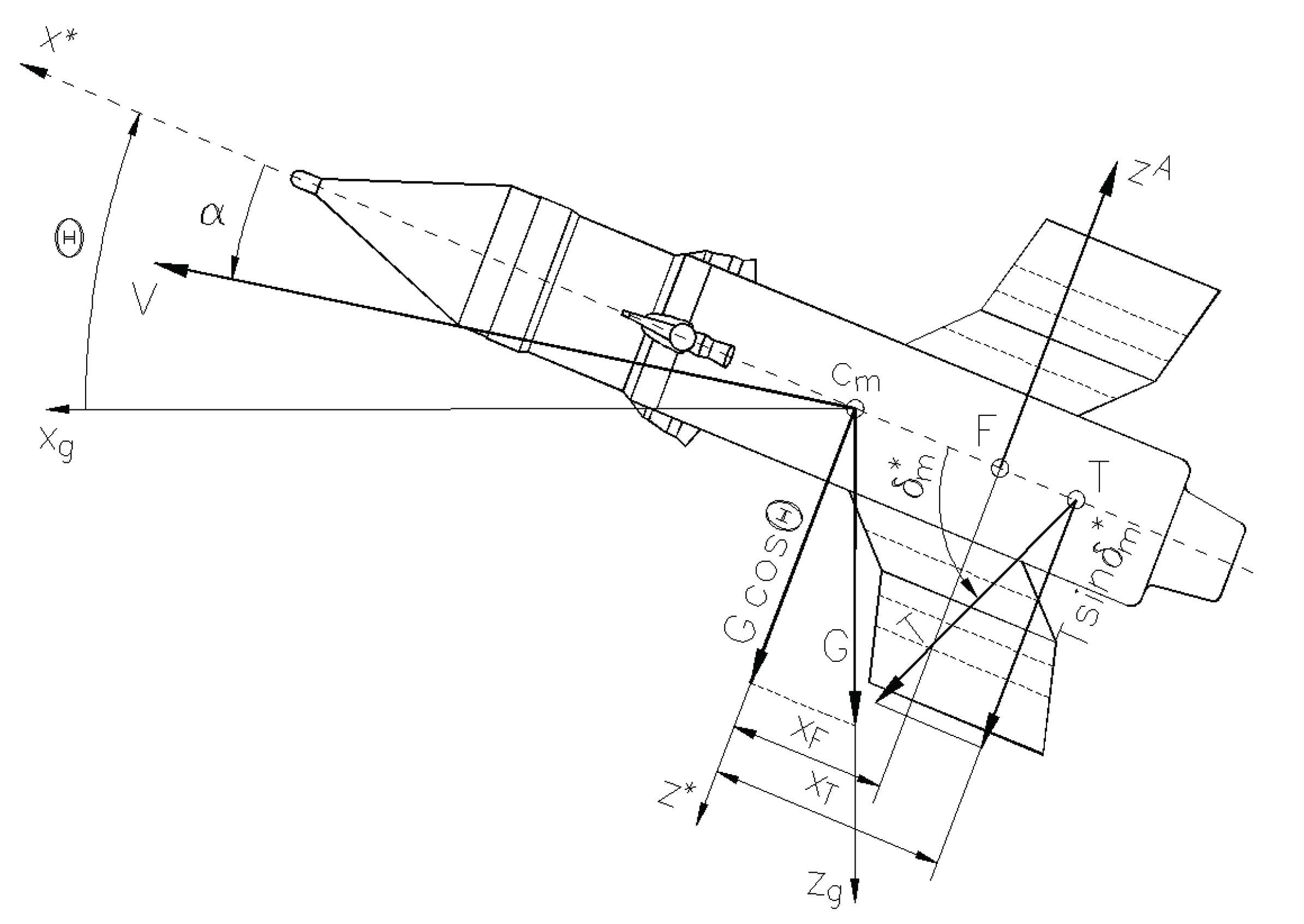
Figure 4.
Equilibrium incidence in the lateral plane.
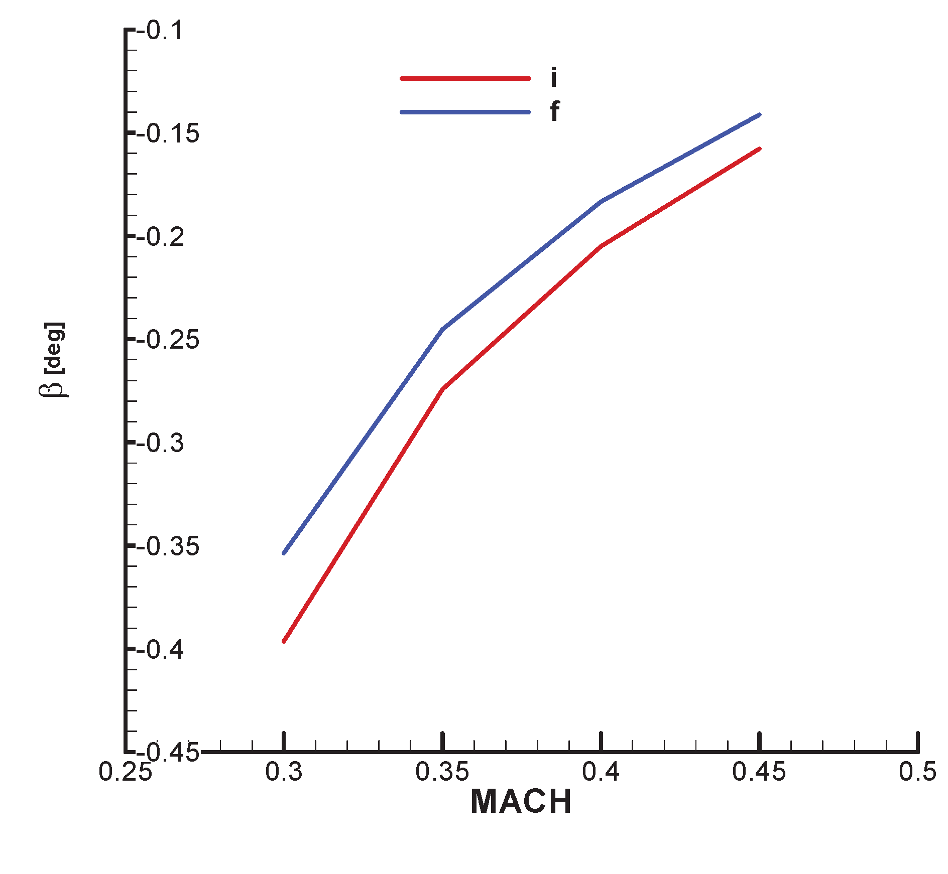
Figure 5.
The roots of the characteristic polynomial -initial.
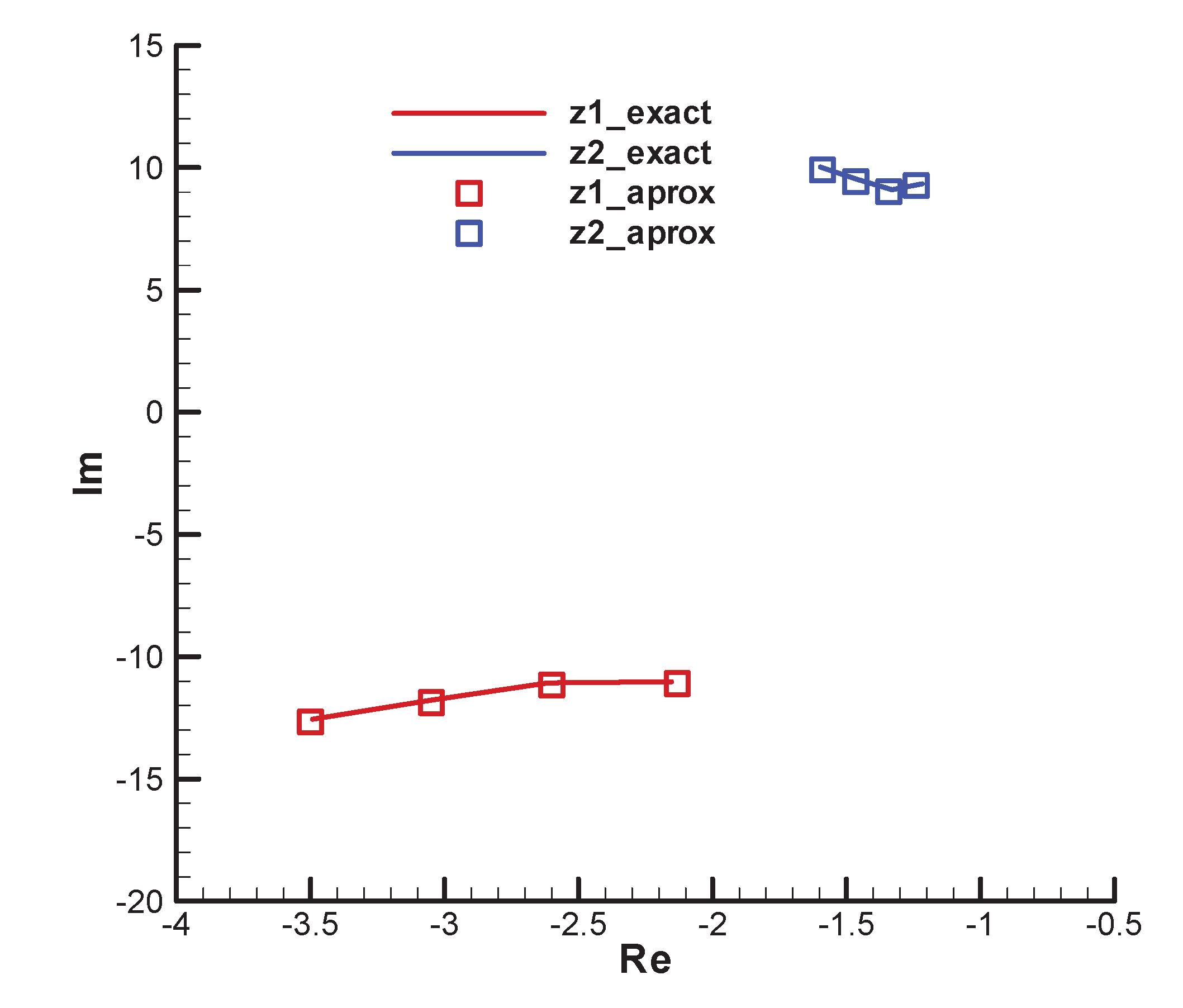
Figure 6.
The roots of the characteristic polynomial -final.

Figure 7.
Structural scheme of commanded movement for a slow-rolling missile
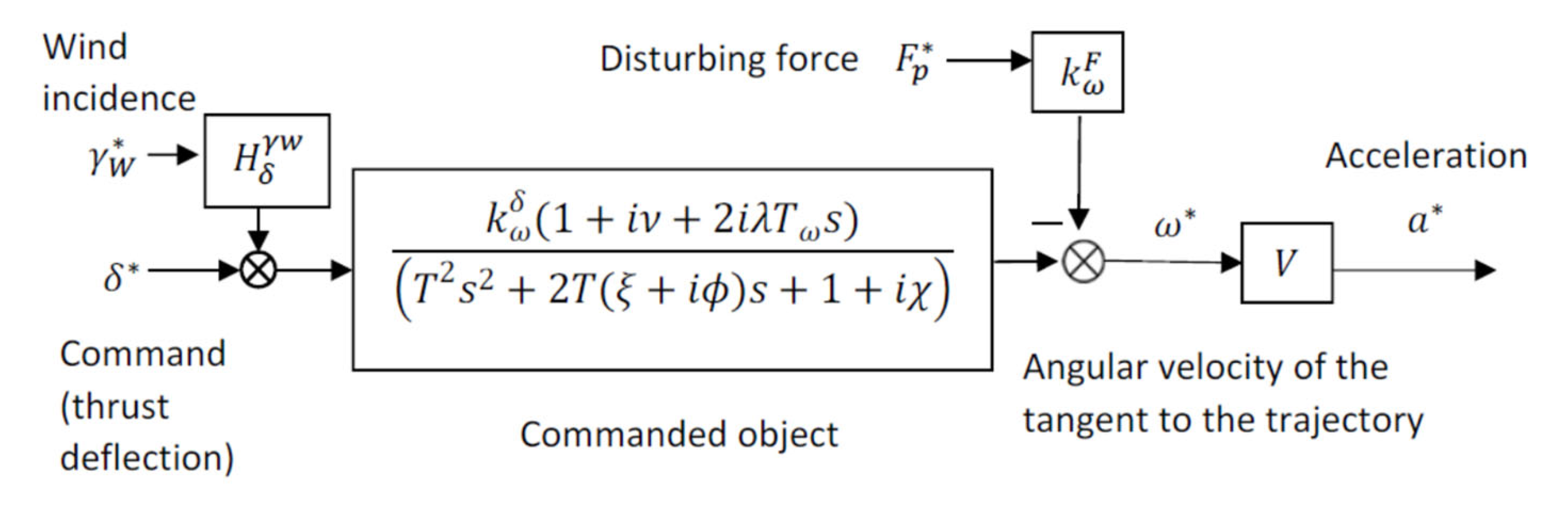
Figure 8.
Orientation of the guiding frame with respect to the local frame [26].
Figure 8.
Orientation of the guiding frame with respect to the local frame [26].
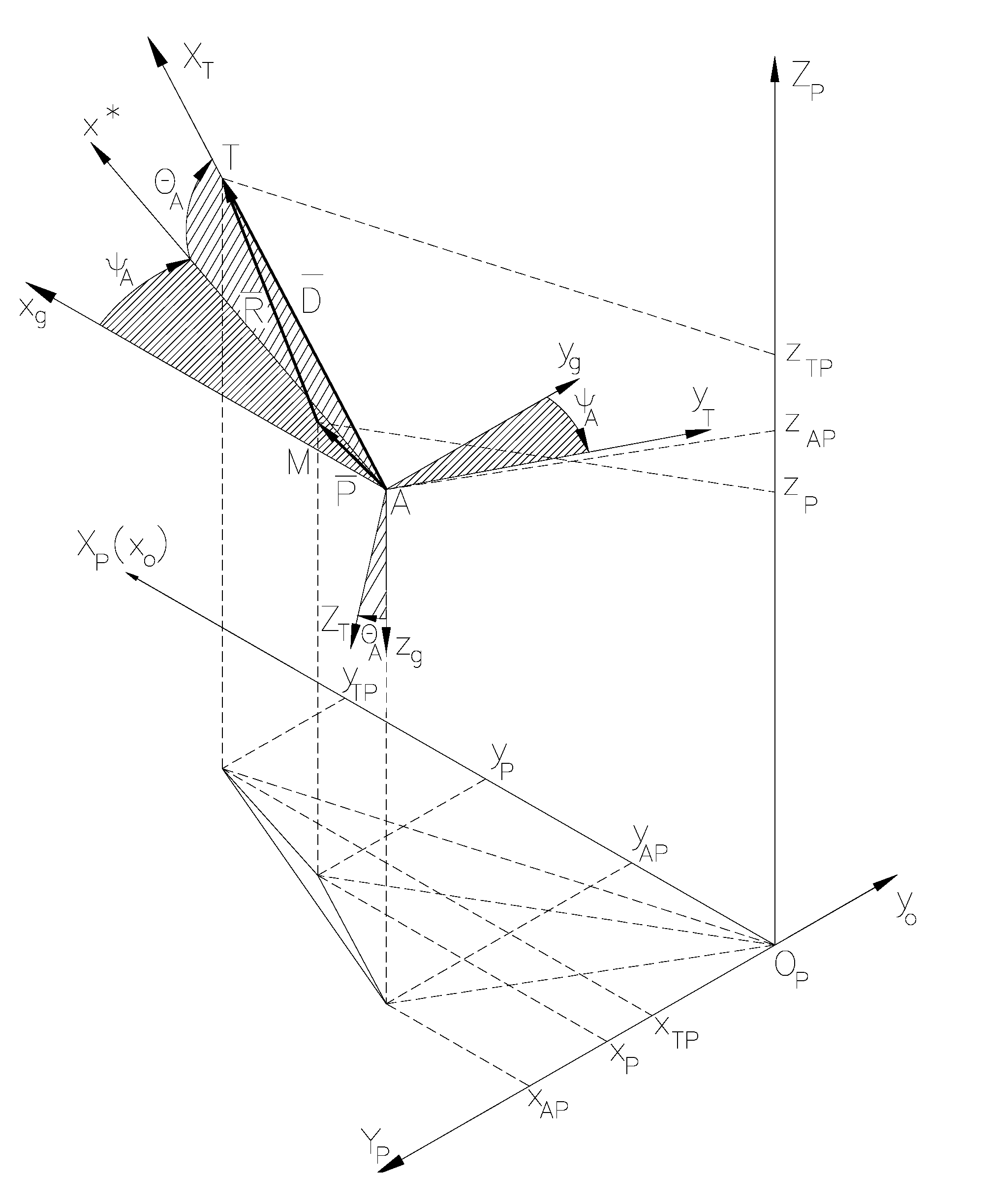
Figure 9.
Kinematics of three-point guidance method - first guiding plane.
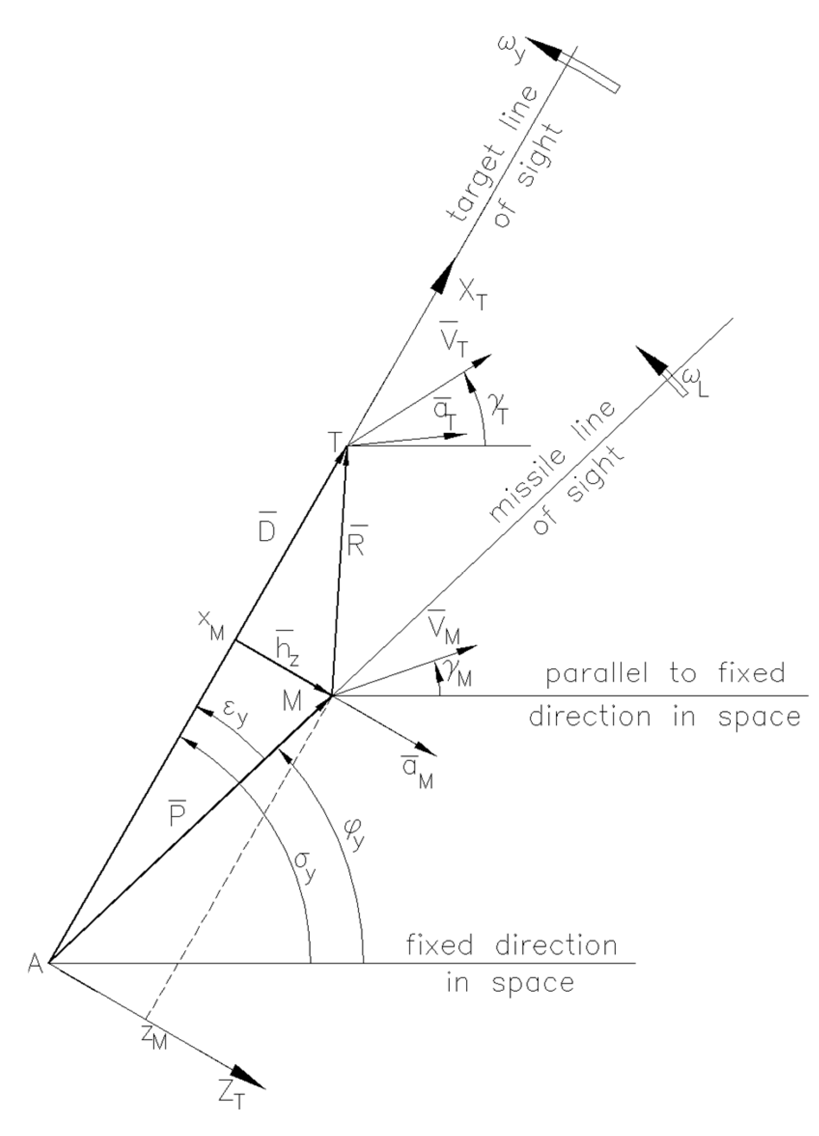
Figure 10.
Kinematics of three-point guidance method - second guiding plane.
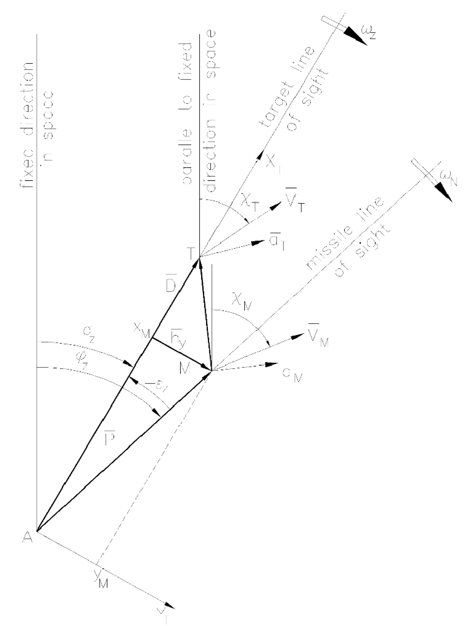
Figure 11.
The guidance command in polar coordinates.
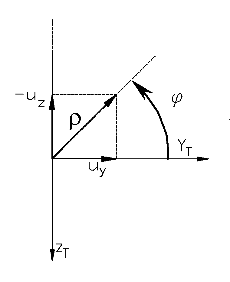
Figure 13.
Rolling missiles with gasodynamic controls.
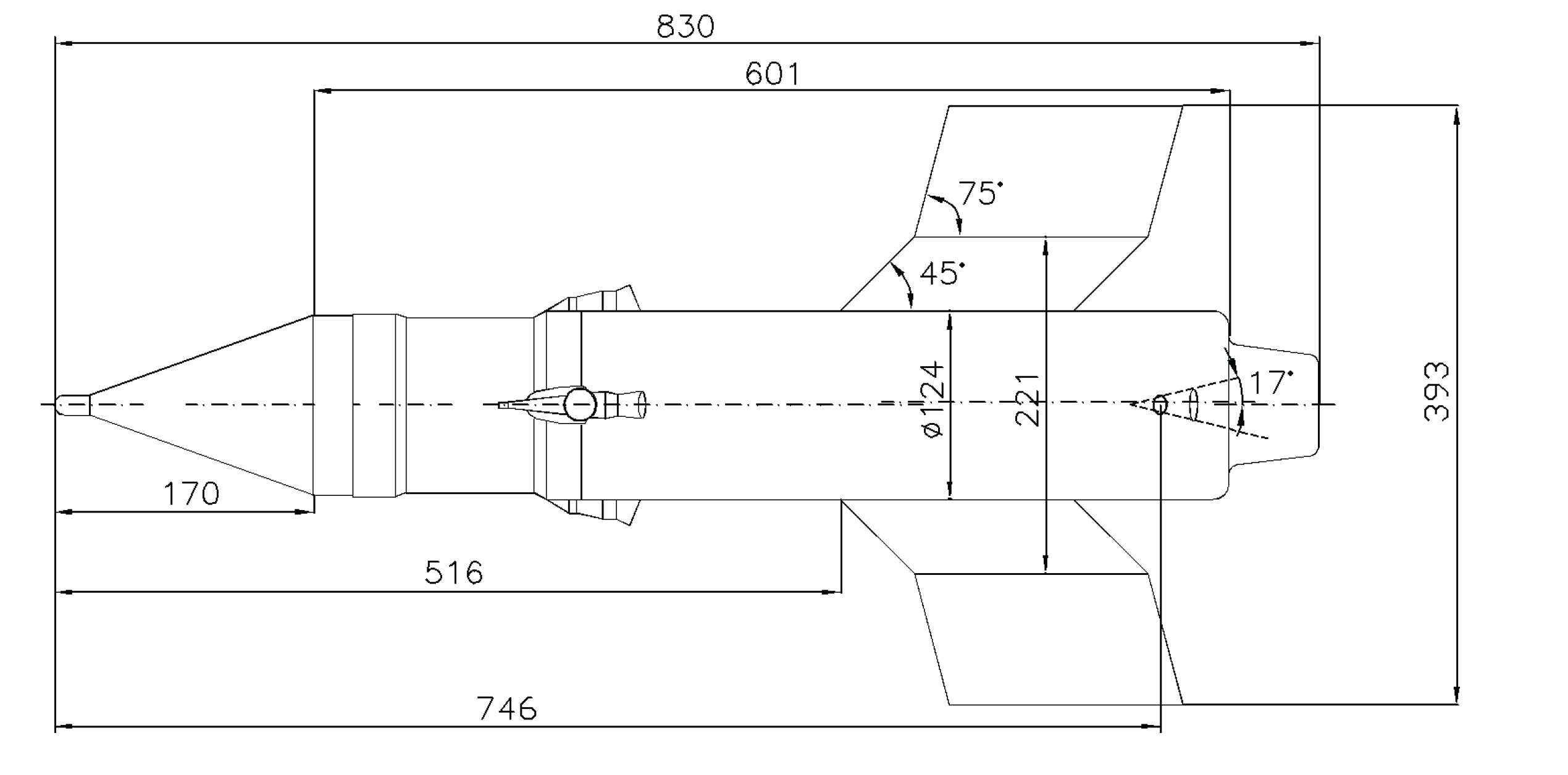
Figure 14.
Thrust diagram.
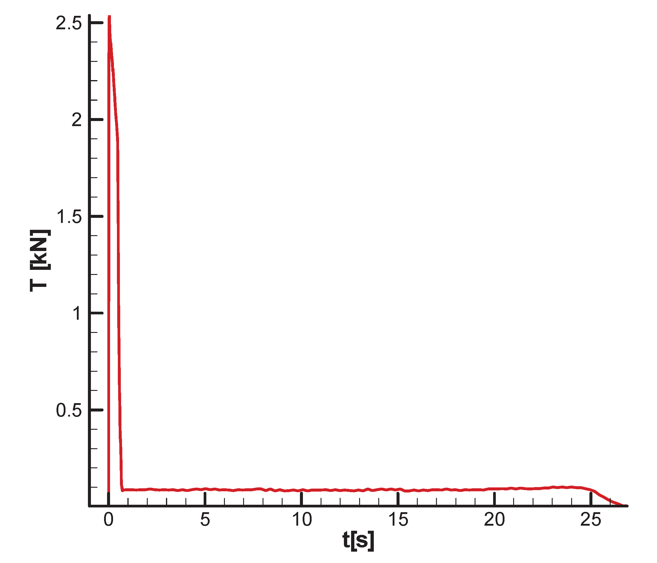
Figure 15.
Stability R-H domains Mach=0.3, - initial.
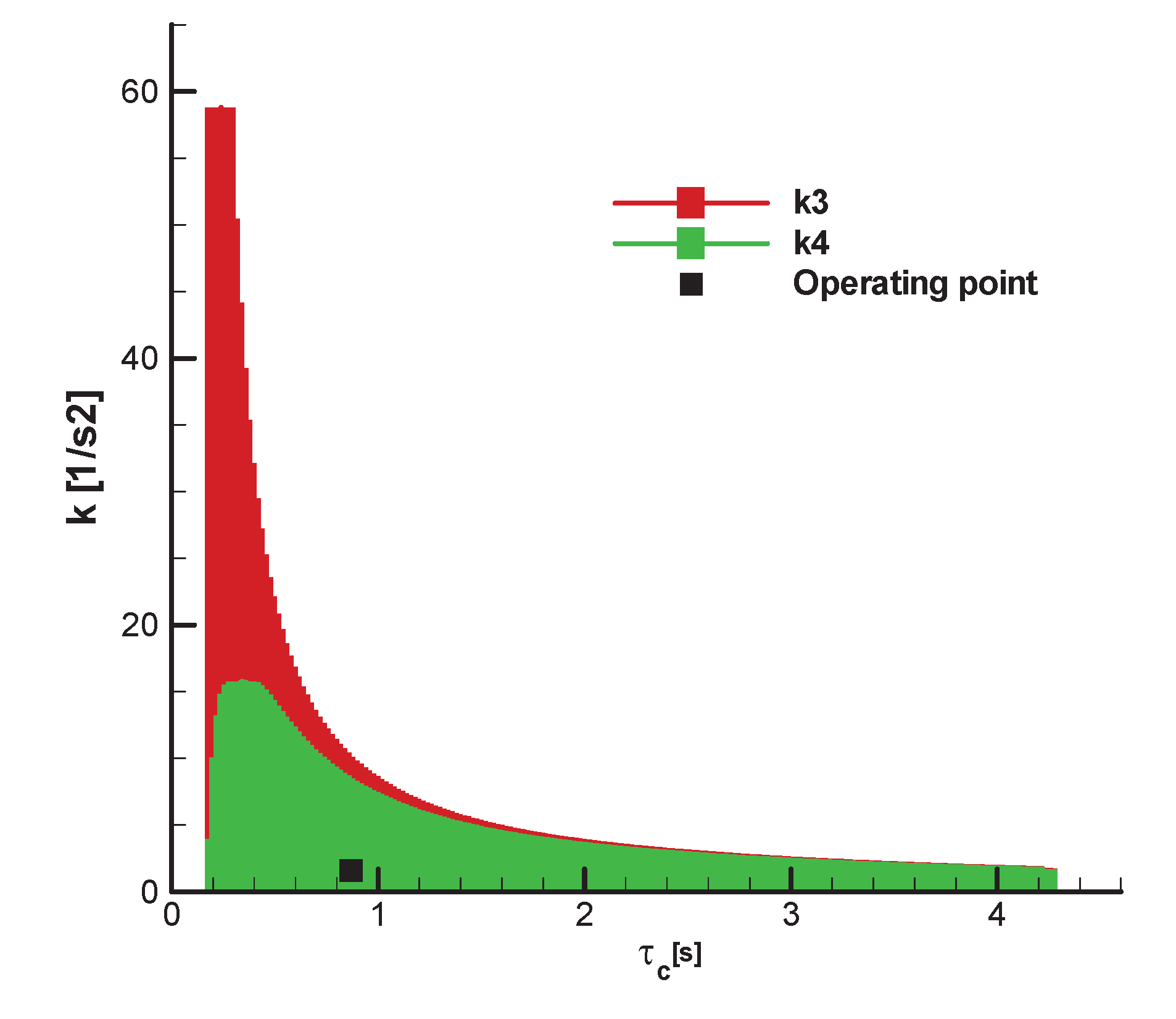
Figure 16.
Stability R-H domains Mach=0.45, – final.
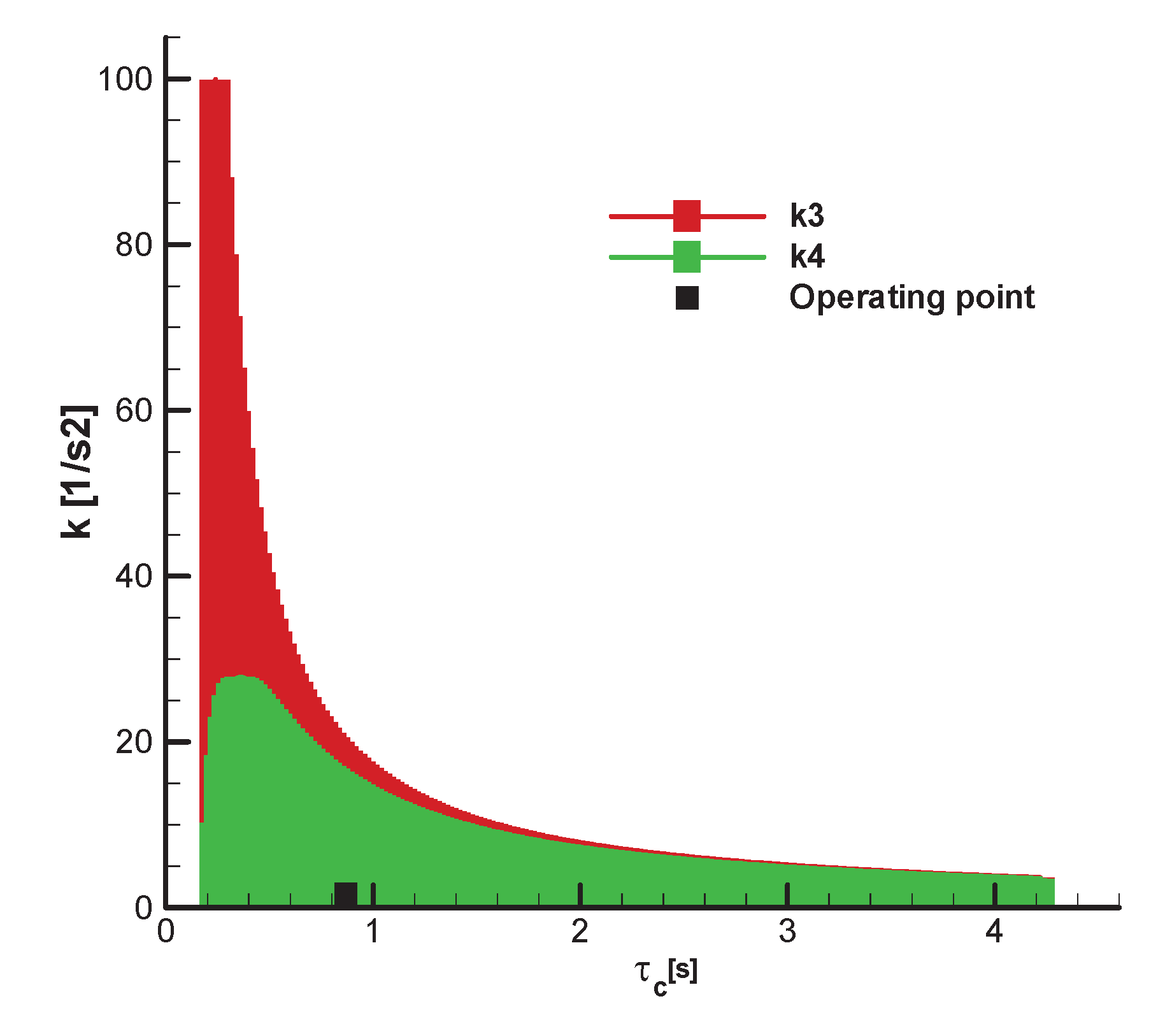
Figure 17.
Upper limits () () and gain (k) - initial;
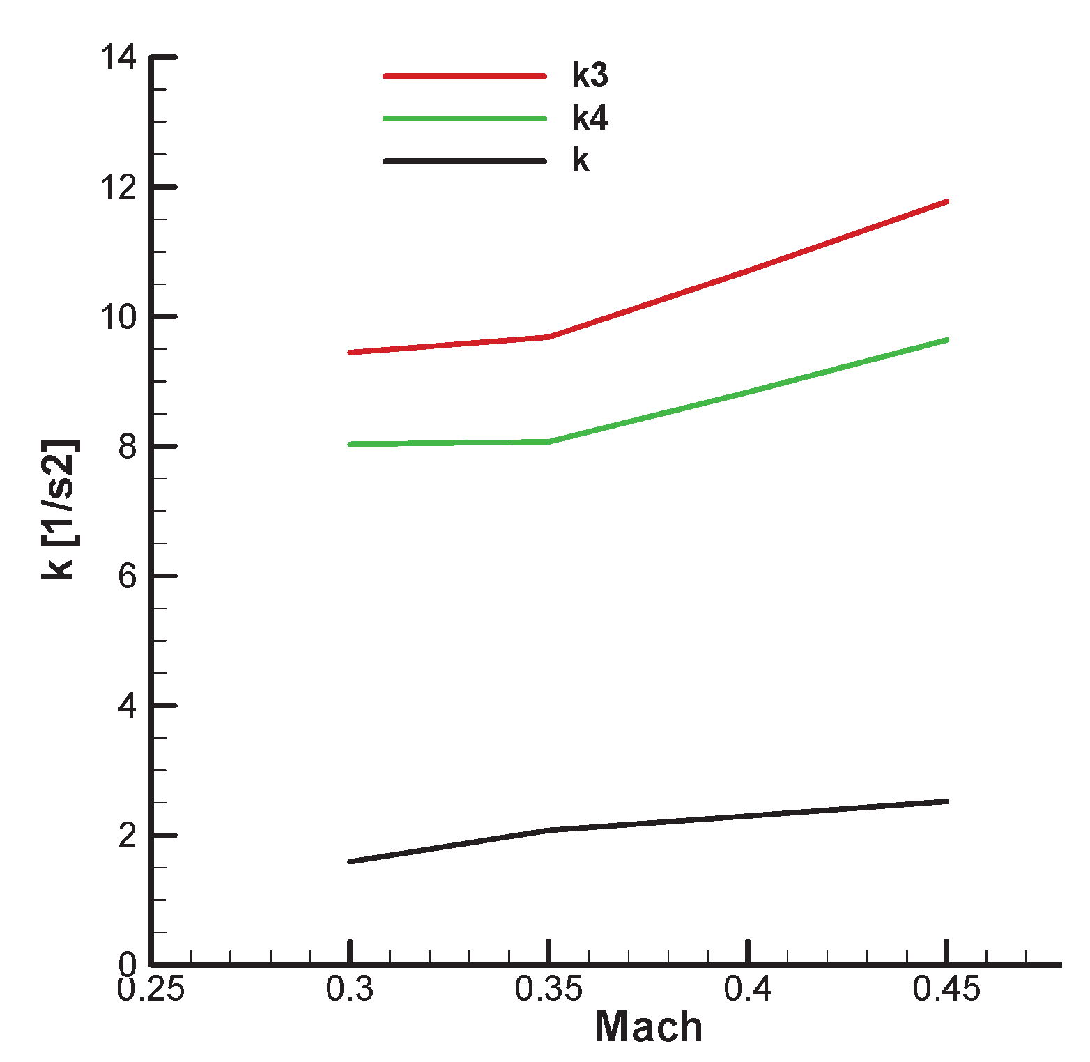
Figure 18.
Upper limits () () and gain (k) - final; Finally, the condition , because we have already imposed the condition leads to , i.e. .
Figure 18.
Upper limits () () and gain (k) - final; Finally, the condition , because we have already imposed the condition leads to , i.e. .
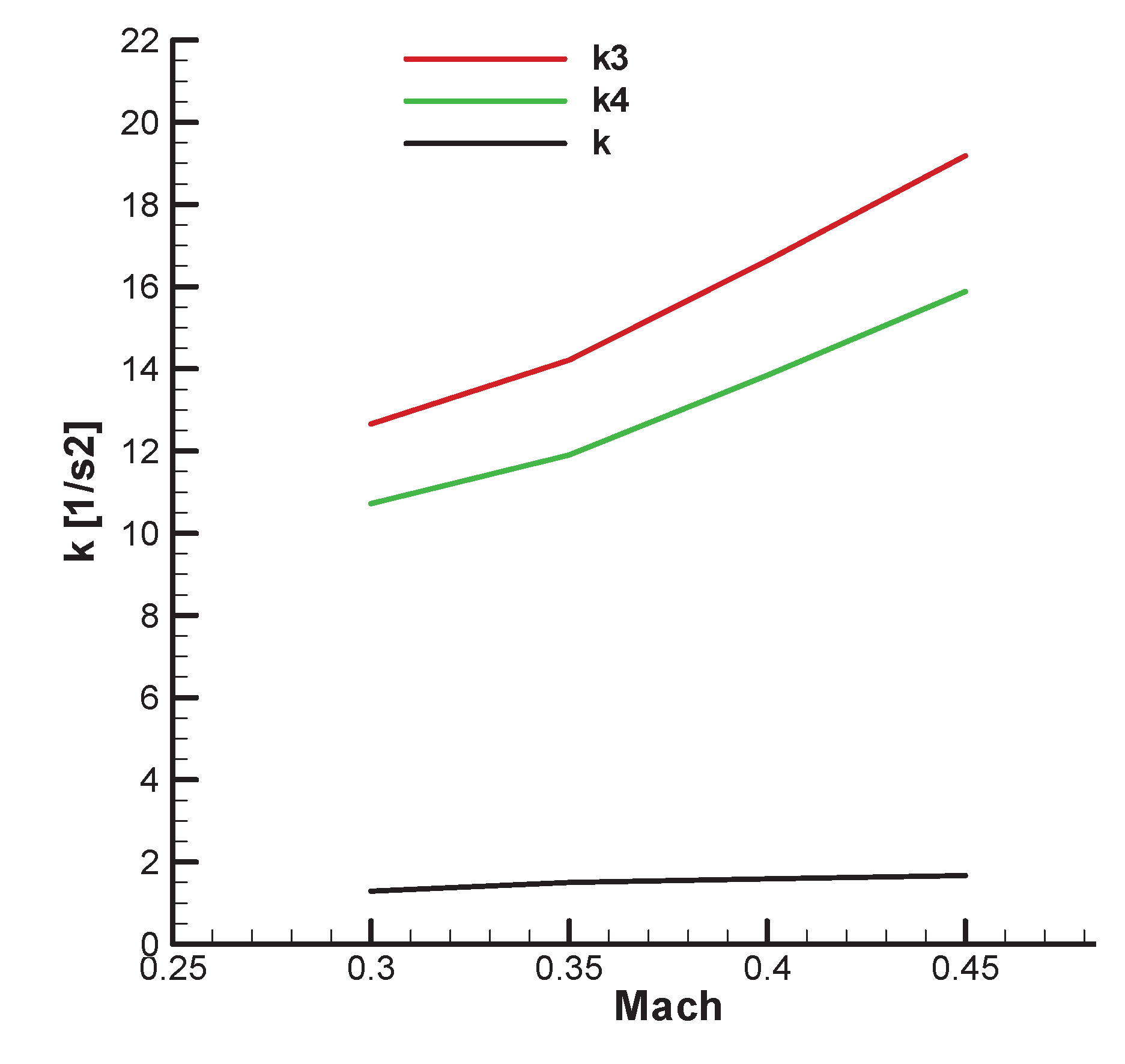
Figure 19.
Variation of the F-W parameters as a function of the guidance gain - initial;
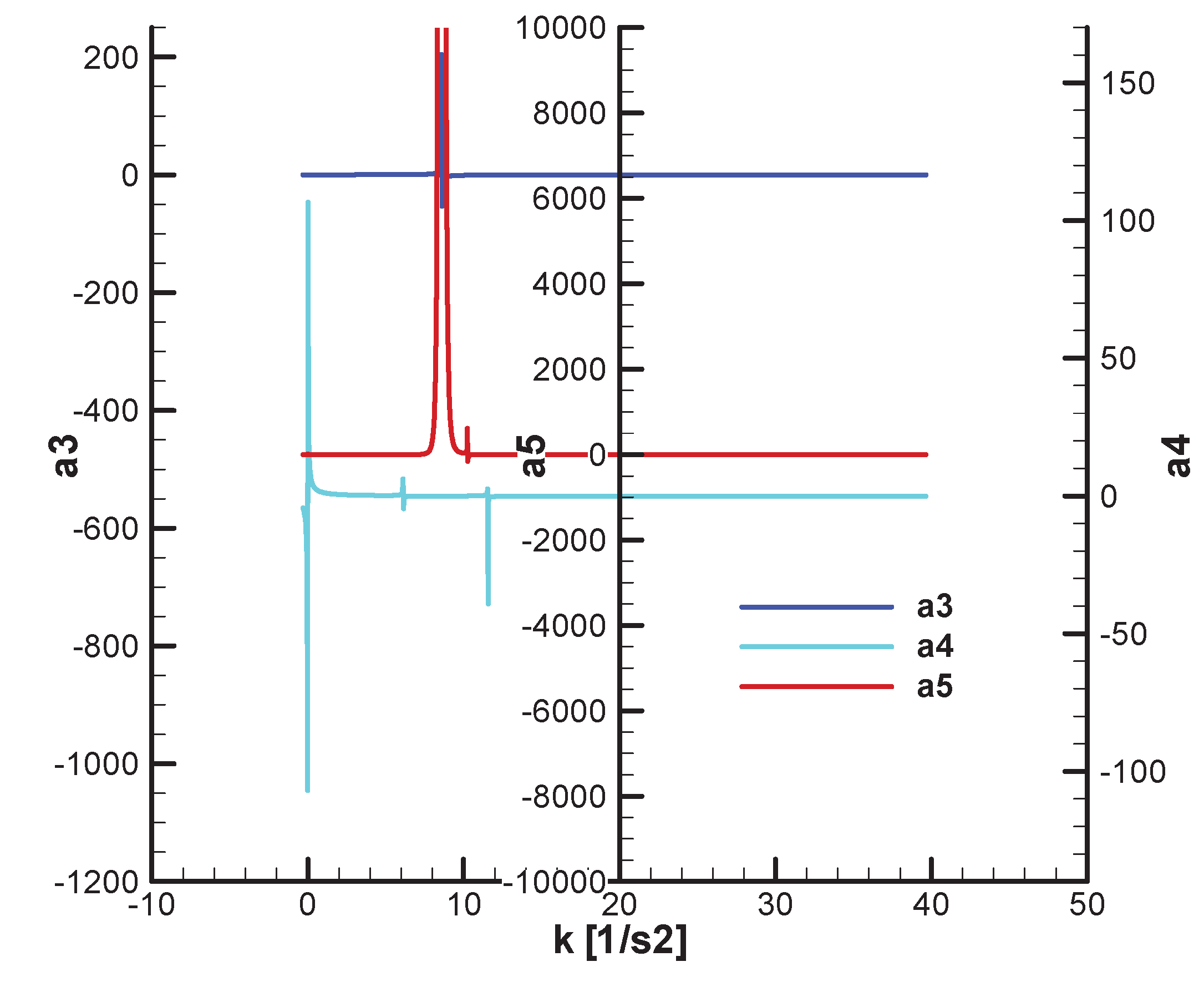
Figure 20.
Variation of the F-W parameters as a function of the guidance gain - initial;
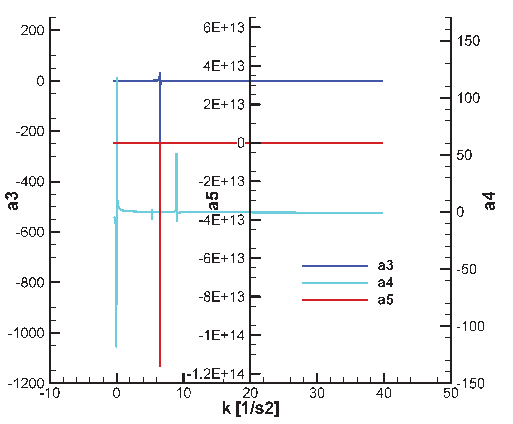
Figure 21.
Variation of the F-W parameters as a function of the guidance gain - final;
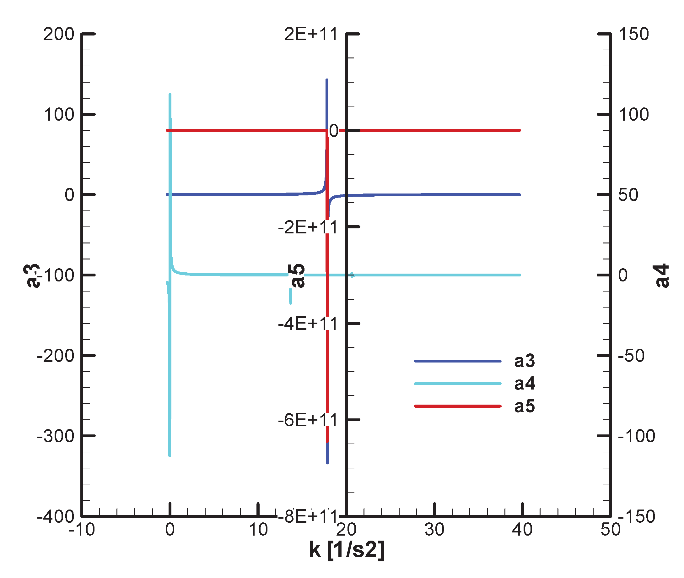
Figure 22.
Variation of the F-W parameters as a function of the guidance gain - final; Figure 23 and Figure 24 the corresponding stability domains for and for fixed at operating point (in the initial and final of the second phase.
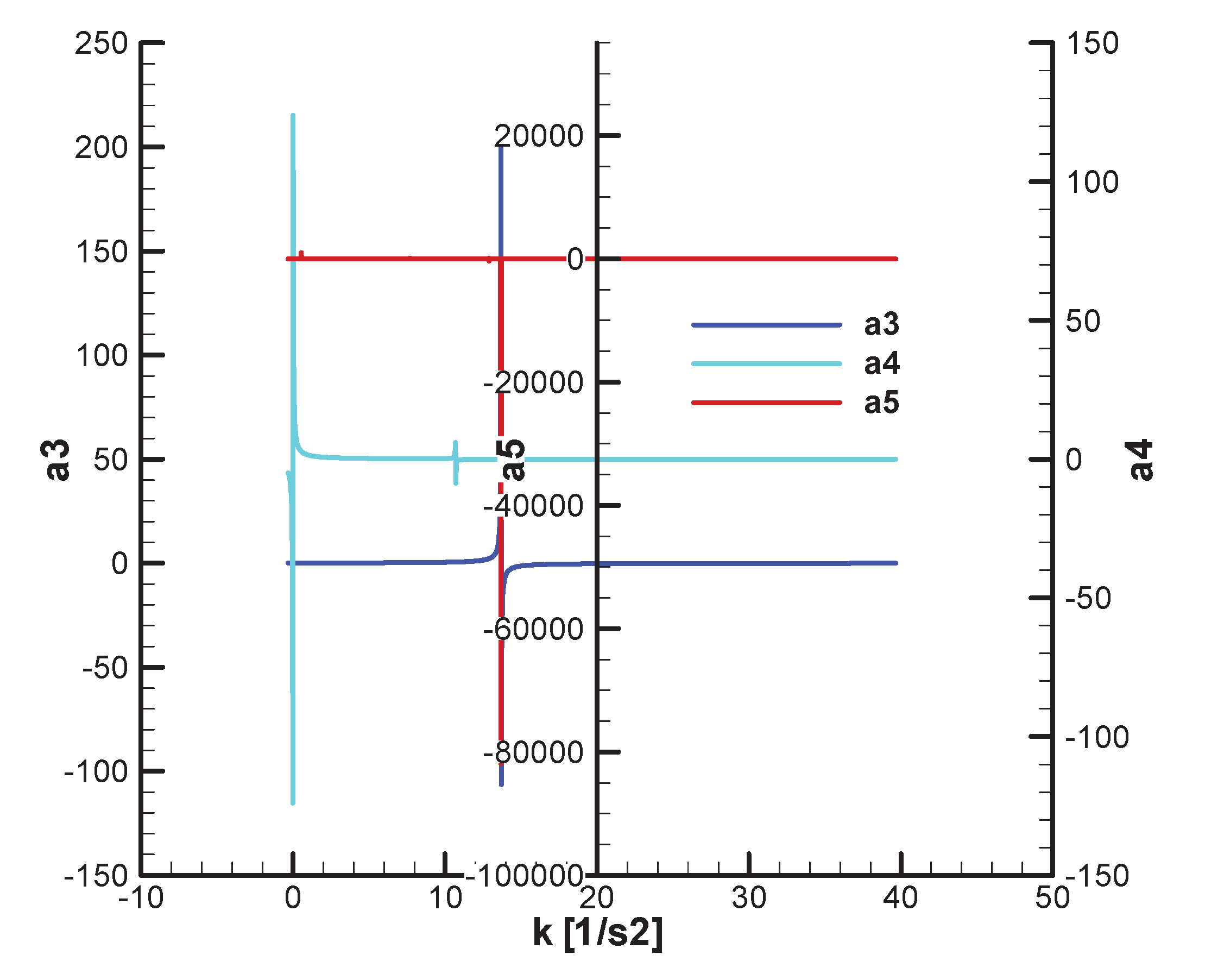
Figure 25.
Stability domains Mach=0.3 ; - initial.
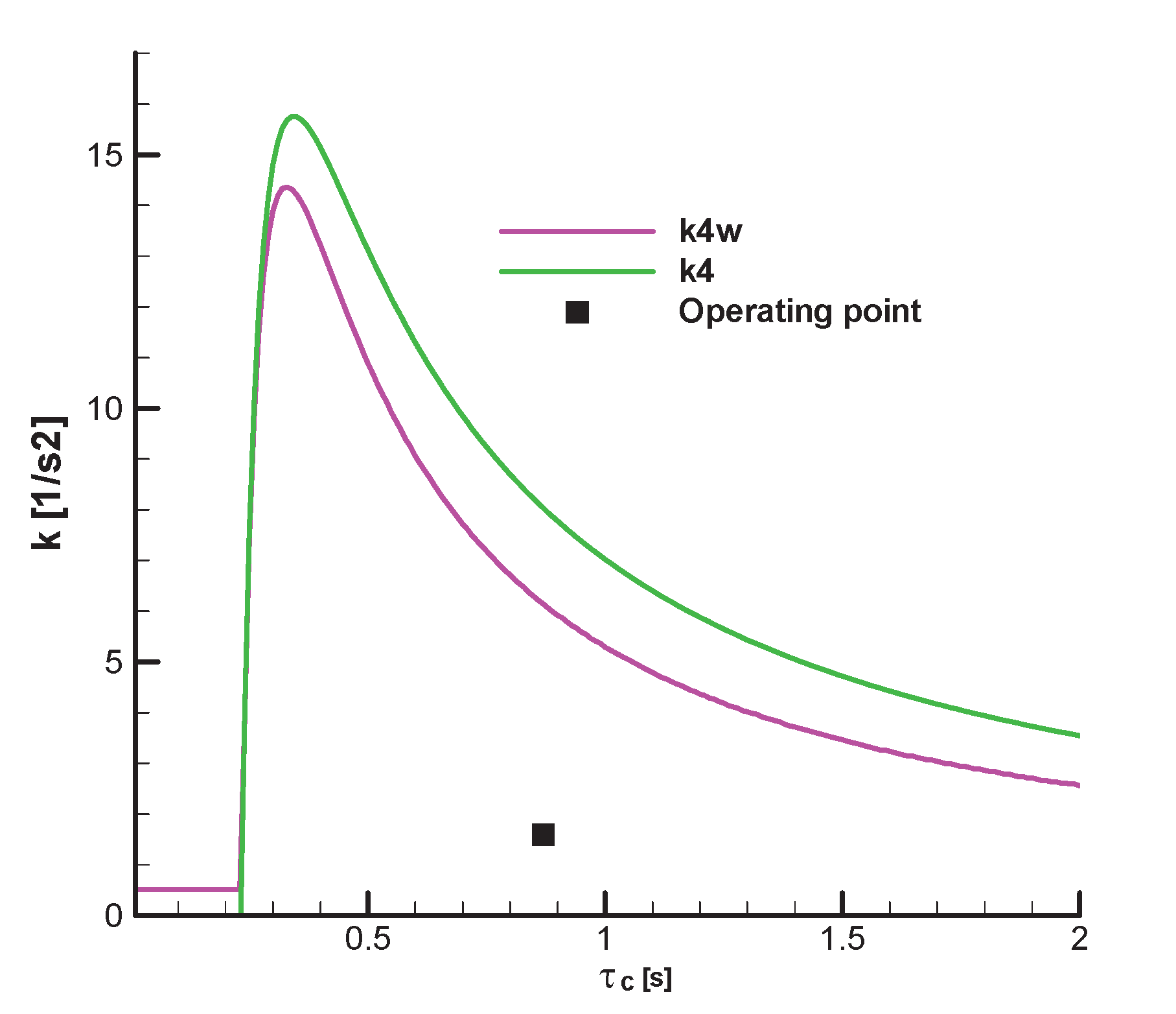
Figure 26.
Stability domains Mach=0.45, – final.
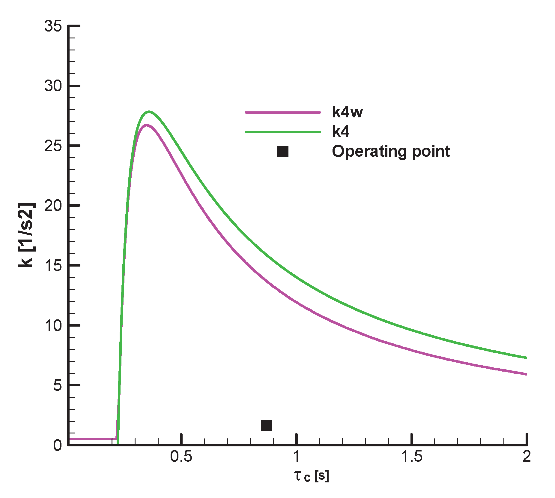
Figure 27.
Stability parameters F-W – initial; ;
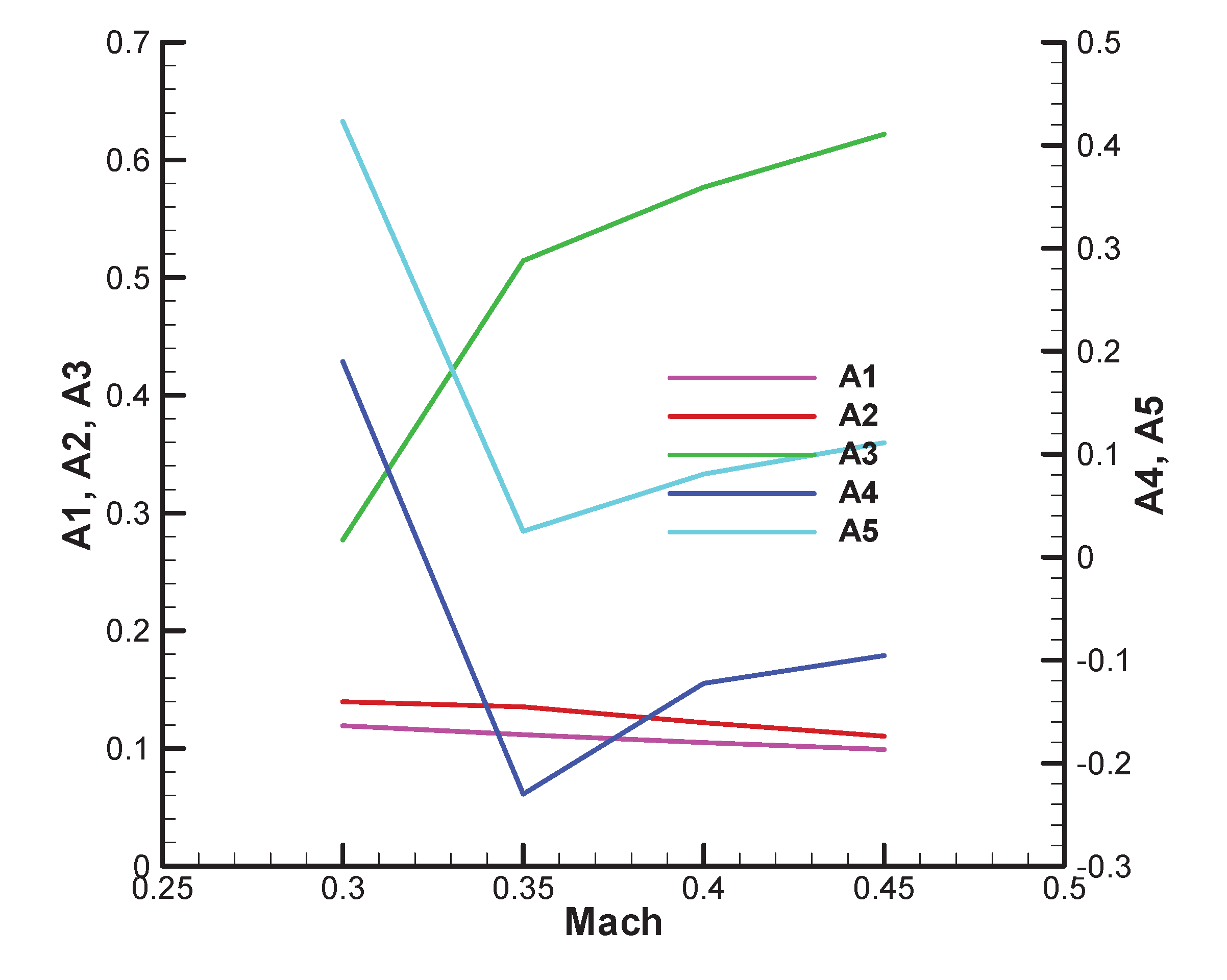
Figure 28.
Roots of the characteristic polynomial with complex coefficients– initial;
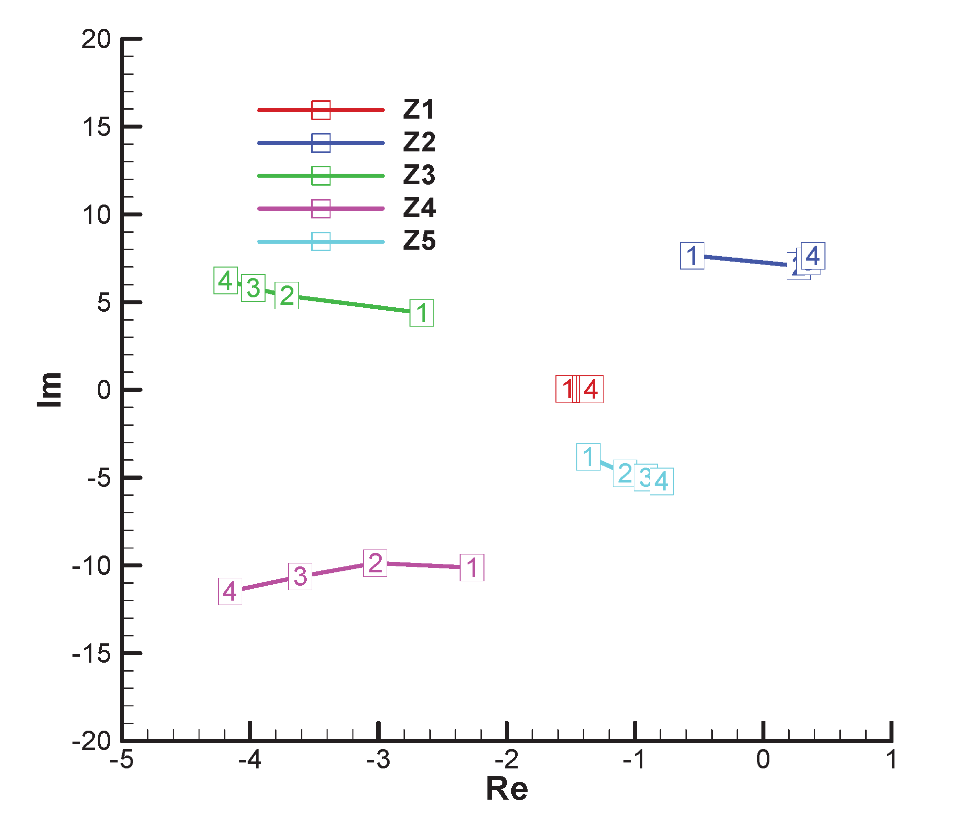
Figure 29.
Upper limits () () and gain (k) – initial;
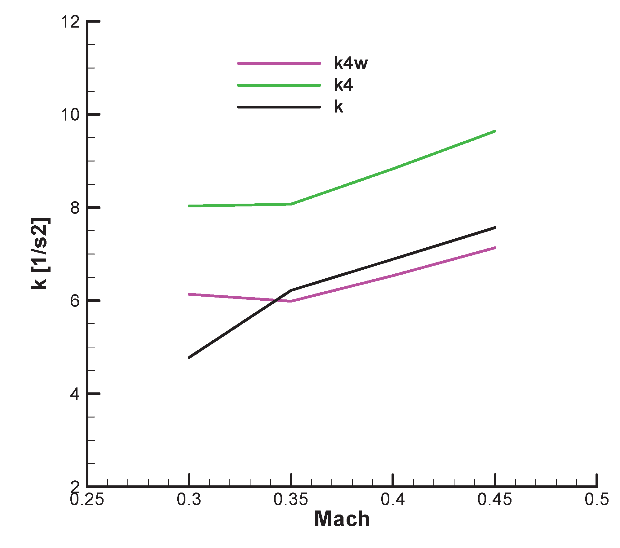
Figure 30.
Roots of the characteristic polynomial with real coefficients – initial

Figure 37.
Target hitting – vertical view; ; ;
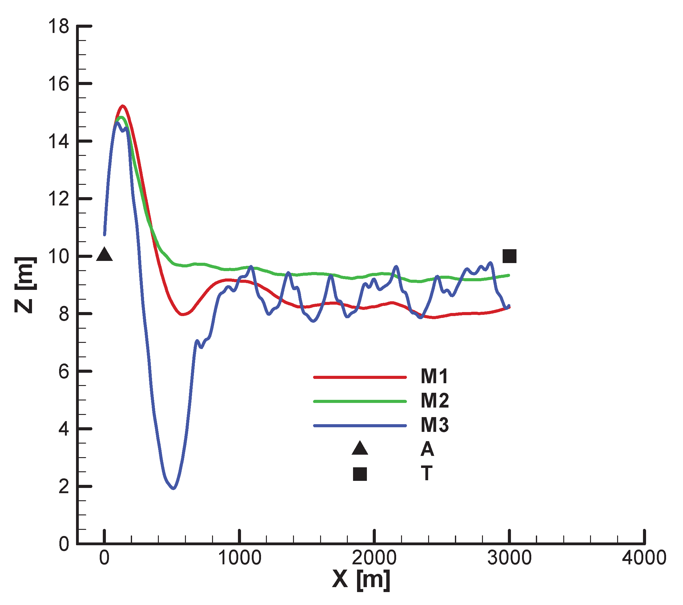
Figure 38.
Target hitting – horizontal view; ;
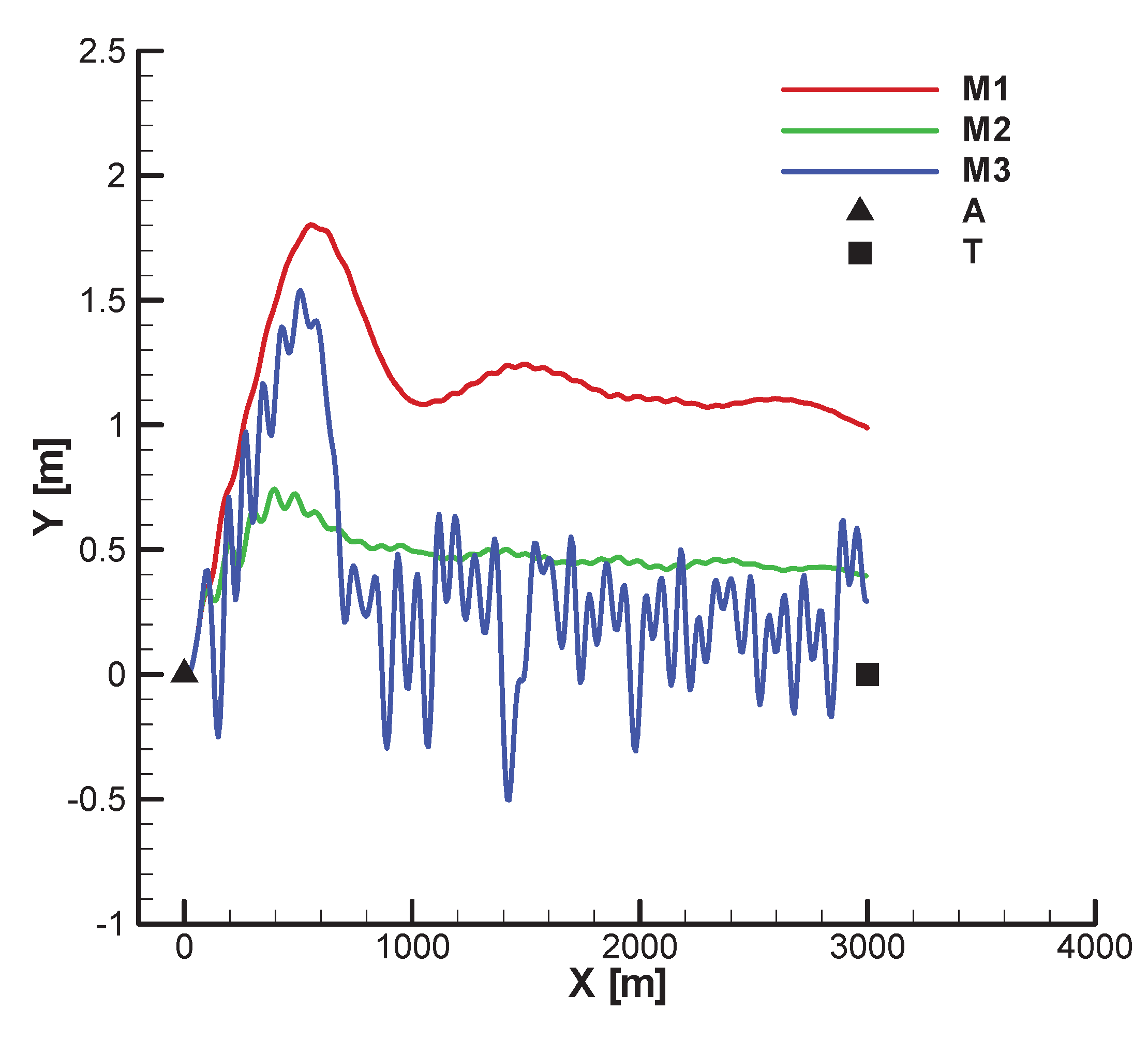
Figure 39.
Target hitting – vertical view; ; ;
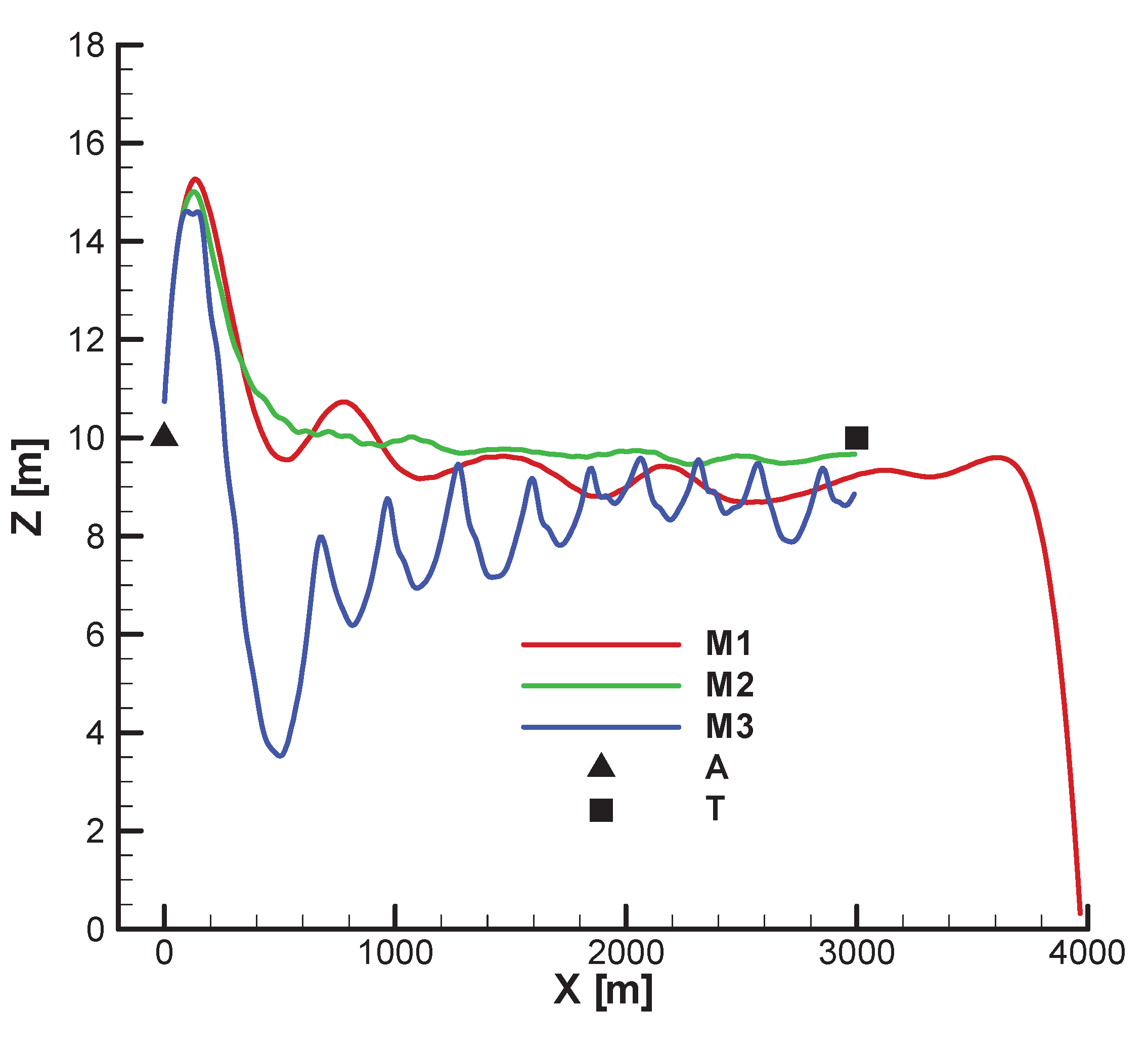
Figure 40.
Target hitteing – horizontal view; ; ;
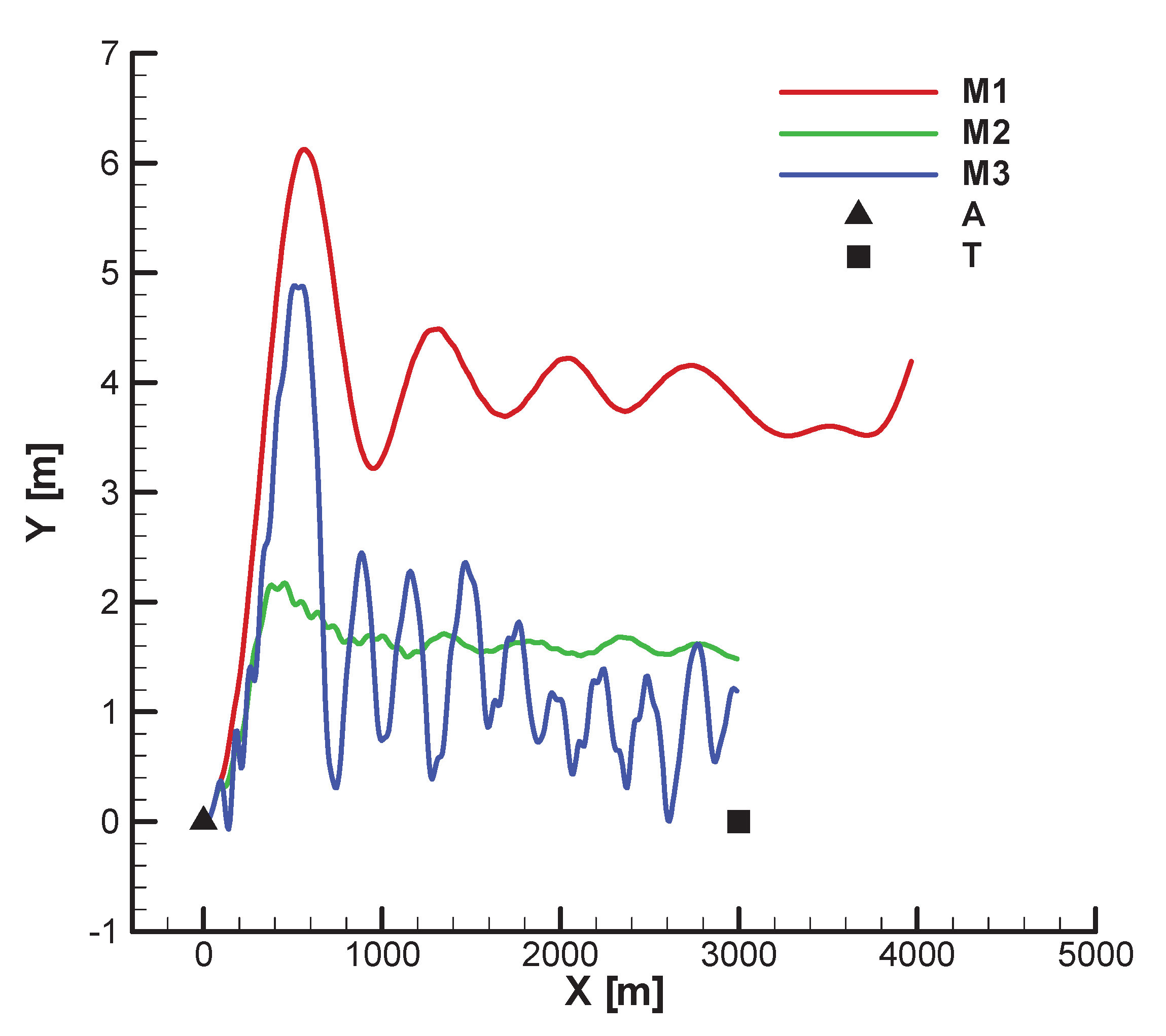
Figure 41.
Command fill factor;
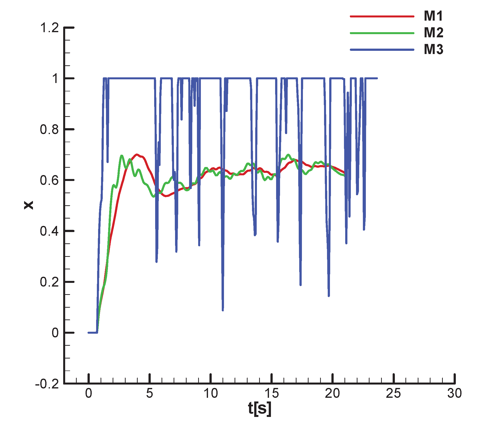
Figure 42.
Coemmand fill factor; ; ;
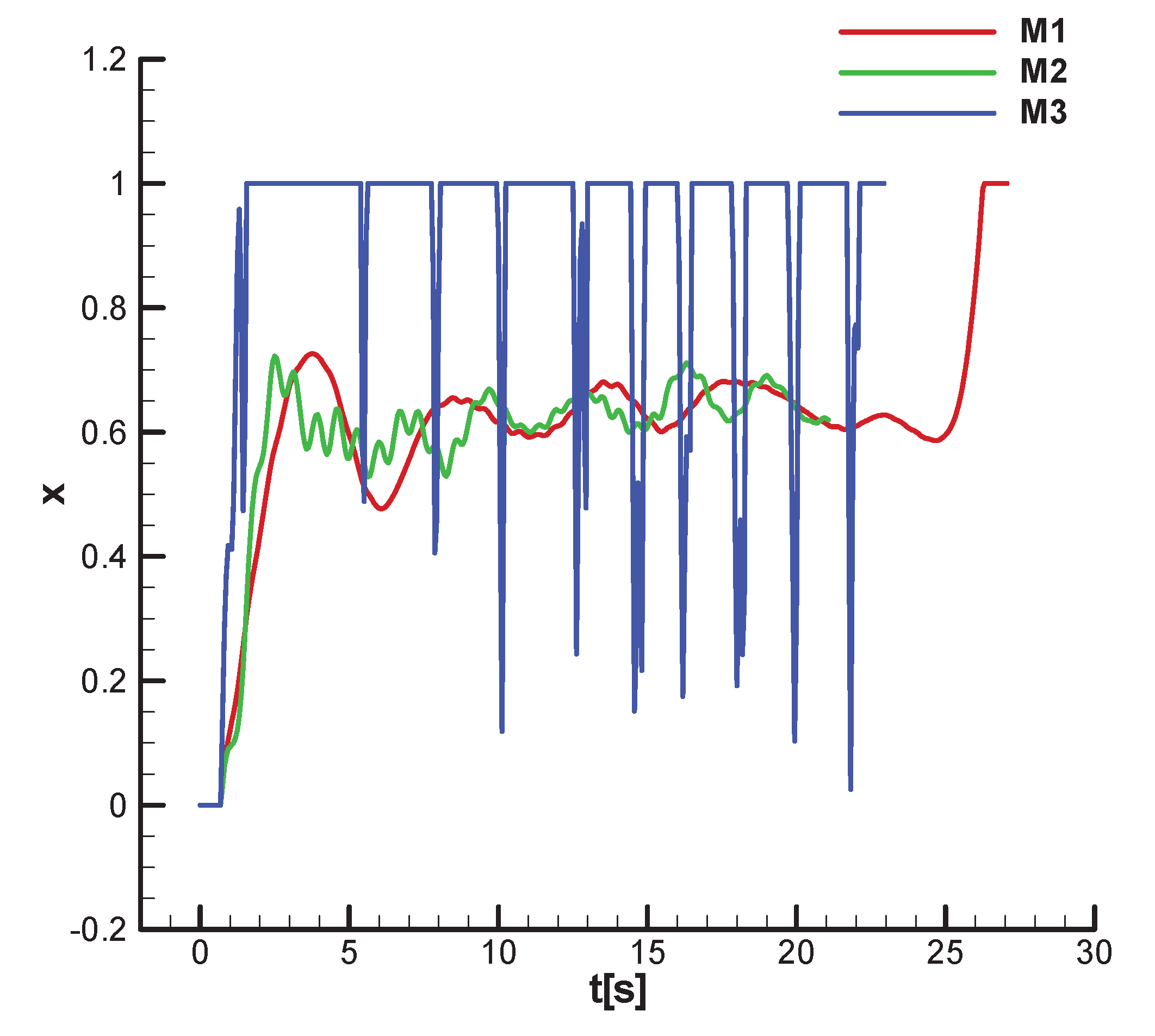
Figure 43.
Command phase; ; ;
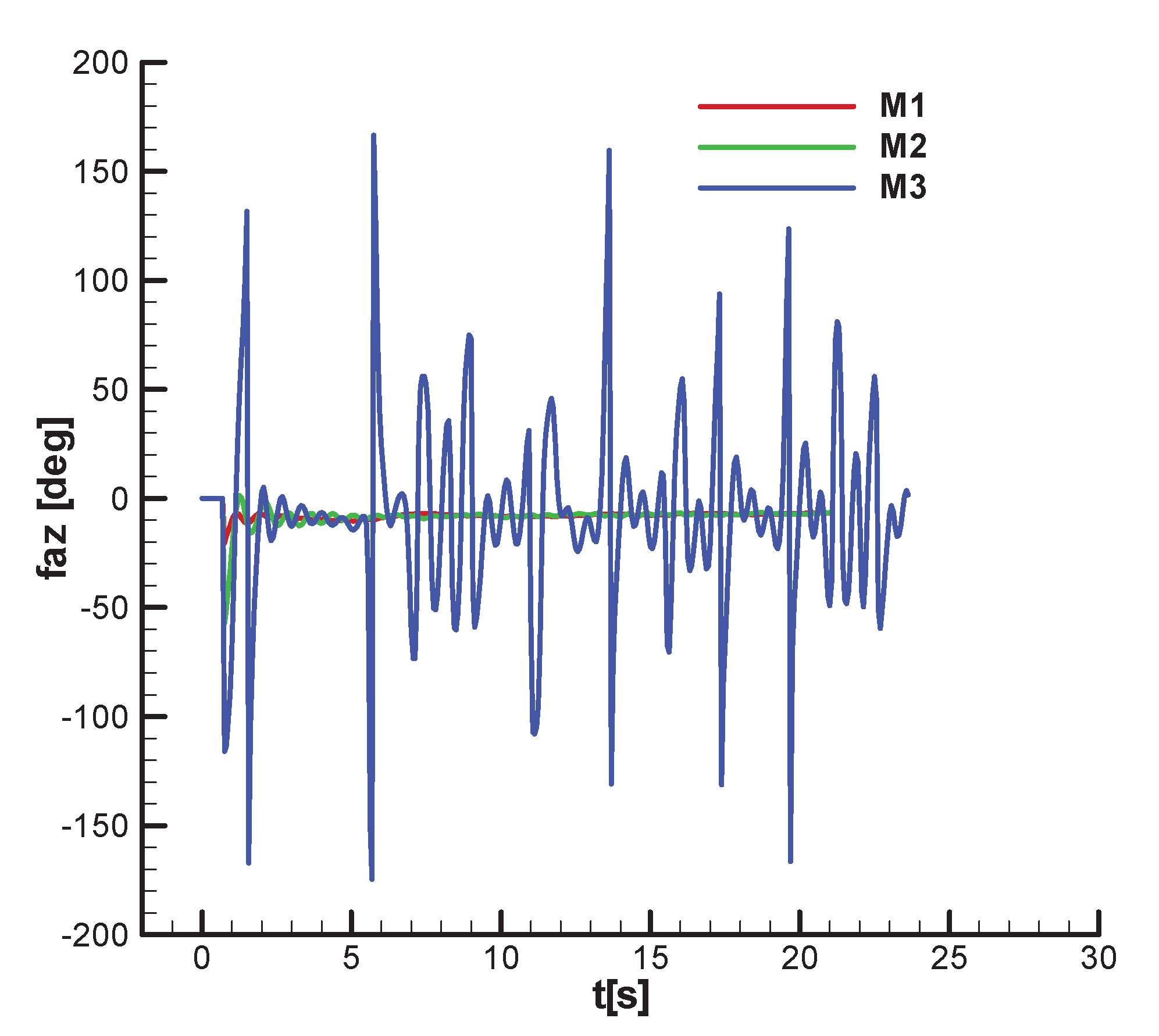
Figure 44.
Command phase; ;
Disclaimer/Publisher’s Note: The statements, opinions and data contained in all publications are solely those of the individual author(s) and contributor(s) and not of MDPI and/or the editor(s). MDPI and/or the editor(s) disclaim responsibility for any injury to people or property resulting from any ideas, methods, instructions or products referred to in the content. |
© 2025 by the authors. Licensee MDPI, Basel, Switzerland. This article is an open access article distributed under the terms and conditions of the Creative Commons Attribution (CC BY) license (http://creativecommons.org/licenses/by/4.0/).
Copyright: This open access article is published under a Creative Commons CC BY 4.0 license, which permit the free download, distribution, and reuse, provided that the author and preprint are cited in any reuse.


