
Submitted:
15 November 2025
Posted:
17 November 2025
You are already at the latest version
Abstract
We develop the Deterministic Statistical Feedback Law (DSFL) as a concrete finite-dimensional framework for quantum information. DSFL works in a single calibrated Hilbert “room”, compares statistical blueprints to physical responses through one residual of sameness, and declares as lawful exactly those updates that contract this residual in a fixed instrument norm. We prove that admissibility of a channel is equivalent to a spectral data–processing inequality and that iterated admissible dynamics admit a Lyapunov-style envelope, with a canonical DSFL clock making the decay of the residual a straight line in semilog coordinates. On bipartite systems we reinterpret standard entanglement proxies, such as negativity, sandwiched Rényi divergences, and trace distance to product form, as correlation residuals that cannot increase under local completely positive maps. Embedding CHSH and GHZ or Mermin tests into the same room, we recover the usual quantum violations while all local hidden-variable models remain confined to their classical bounds.
Keywords:
DSFL
; admissibility
; data–processing inequality
; Lyapunov envelope
; quantum channels
; entanglement
; bell inequalities
; Hilbert–space geometry
1. Introduction
Any serious attempt to understand entanglement has to separate the correlations we actually observe from the formal machinery we use to compute them. It is not obvious that the wave function should be treated as a physical object rather than as a compact encoding of conditional statistics. Likewise, the Born rule can be read either as a primitive axiom—“outcome frequencies are given by ”—or as a hint of a deeper structure: perhaps is the unique way a single underlying degree of freedom can distribute a finite “sameness budget” across outcomes, so as to reduce a calibrated mismatch between a statistical blueprint and a physical response. The aim of the present paper is to push this second reading as far as we can in finite dimensions, and to ask whether a single residual law can simultaneously govern channels, entanglement, and Bell nonlocality.
The standard formalism of quantum mechanics assigns to every system a state, usually represented by a density operator or wave function, and to every observable a Hermitian operator acting on a Hilbert space. From these data one computes expectation values, correlation functions, and violations of Bell inequalities. In practice this machinery is extraordinarily successful: entangled states are routinely prepared and used as resources for quantum teleportation of unknown states, device–independent cryptography, and quantum communication in ways that cannot be reproduced by shared classical randomness alone [1,2,3,4]. From a logical point of view, this success still leaves open a question that goes back to Einstein, Podolsky, and Rosen [5]: is the quantum formalism merely empirically correct, or is it also complete?
Bell’s theorem and the experiments that followed show that entangled correlations are incompatible with any local hidden–variable description [4,6,7,8,9]. In that narrow sense, the search for a classical completion has failed: no assignment of pre–existing local values reproduces all quantum predictions. But the completeness question is older and more basic. It asks whether there is a single, transparent law that explains why these correlations have the structure they do, and how they should evolve under general dynamics, rather than just a collection of separate calculation rules and monotonicity theorems.
In its sharpest form, the Einstein–Podolsky–Rosen question can be rephrased as follows. Given a theory we accept as empirically correct, does every element of physical reality have a clear counterpart in its mathematical description, and does that description come with a well–defined arrow of time? For entanglement, this would mean more than having many inequivalent measures and criteria. It would mean that there is a single quantity, or a tightly controlled family of quantities, whose behaviour under admissible dynamics captures what is meant by “nonclassical correlation’’. At present the situation is more fragmented. In quantum information, entanglement is organised into resource theories and manipulated by LOCC maps [3]. In open quantum systems, the natural language is that of completely positive maps and Lindblad or GKSL equations [10,11,12], with contractive norms as a key property. Bell tests are phrased in terms of probability polytopes and correlation functions [4], largely decoupled from the dynamical structure of channels and instruments. Negativity, sandwiched Rényi divergences, and trace distance to product states reappear in the context of hypothesis testing, thermodynamics, and information theory [13,14,15]. Each viewpoint is powerful, but they do not obviously form a single, law–like whole.
The Deterministic Statistical Feedback Law (DSFL) is an attempt to provide such a law. The basic idea is to work in one Hilbert room and to compare a statistical blueprint with a physical response by means of a single residual of sameness. Informally, one thinks of the blueprint as “what the device thinks it is doing” (settings, control parameters, intended state) and the response as “what actually happens in the apparatus or in the world”. DSFL then tracks, in one fixed norm, how far the response is from the calibrated image of the blueprint, and declares as lawful exactly those evolutions that do not increase this discrepancy.
Concretely, we fix:
- a statistical space of blueprints (statistical degrees of freedom, sDoF), carrying the variables that describe preparations, control knobs, and intended states;
- a physical space of responses (physical degrees of freedom, pDoF), carrying the variables that describe actual readouts, fields, or detector states;
- a calibration map , which tells us, for each blueprint , what the ideal response in would be if the device were perfectly implemented; and
- an instrument weight on , which encodes how the instrument “measures distance” between two responses via the norm .
Given a blueprint–response pair , the DSFL residual of sameness is the single scalar
i.e. the squared distance, in the instrument norm, between the actual response p and the calibrated ideal response . In DSFL this quantity plays the central rôle: it is the only observable we track for lawfulness (via a data–processing inequality), for dynamics (via Lyapunov decay), and for locality (via cone bounds), and all sectors of the theory are required to respect the same residual .
Admissible evolutions are precisely those that contract this residual in the instrument norm. In finite dimension this is equivalent to a spectral data–processing inequality of the form , and plays the rôle of a Lyapunov function with a printed decay rate. In this sense DSFL proposes a very simple arrow of time: in an admissible world the calibrated mismatch between blueprint and response is nonincreasing and, where a local margin exists, decays exponentially. At the level of broad ideas, DSFL has been suggested as a common geometric framework in which quantum mechanics, thermodynamics, and even gravitational sectors can be expressed in terms of one residual, one admissibility (DPI) gate, one Lyapunov envelope, and one causal cone.
The aim of the present paper is to confront this proposal with some of the sharpest tests from finite–dimensional quantum information theory: entanglement monotones and Bell inequalities for small systems (a few qubits).[2,3,4] We deliberately restrict attention to finite–dimensional Hilbert spaces and familiar scenarios such as CHSH[4,7] and GHZ/Mermin experiments.[16,17] Within this setting we ask three concrete questions:
- (Q1)
- Channels. Can DSFL be realised as a genuine Lyapunov law for finite–dimensional quantum channels, with admissibility exactly equivalent to a spectral data–processing condition in a fixed instrument norm?
- (Q2)
- (Q3)
Our main conclusion is that, in this finite–dimensional setting, the answer to all three questions is yes. Once a qubit sector is calibrated in a DSFL room, the residual can be treated as the relevant “element of reality’’ for correlations in that sector: its contraction expresses admissibility, its level sets distinguish separable from entangled states (via correlation residuals), and its geometry supports Bell violations up to the Tsirelson bounds [18]. In particular, DSFL reproduces the usual quantum CHSH and GHZ/Mermin values for suitably chosen channels and measurements, while a brute–force enumeration of deterministic local hidden–variable assignments confirms that no classical model within the same framework exceeds the classical bounds [4].
On the Einstein–Podolsky–Rosen question, our answer is therefore twofold. The bare wave–function description, by itself, is not complete in the DSFL sense: it does not single out a residual or a law of admissible contraction. But once the wave function is supplemented by a calibration map, an instrument norm, and the DSFL admissibility condition, we obtain a simple, explicit residual law that is compatible with known entanglement phenomena and Bell nonlocality [3,4], without reverting to local hidden variables. In this qualified sense, DSFL offers a candidate for a more complete description of the physical reality underlying entangled quantum systems. DSFL is not a local hidden-variable theory and does not alter any finite-dimensional quantum predictions; it reorganises the standard formalism into a single residual/DPI/Lyapunov/cone structure.
1.1. Main Idea and Contributions
Informally, the main idea is simple: we take the DSFL residual
seriously as the dynamical object and show that, in small finite dimension, it can simultaneously (a) act as a Lyapunov function for quantum channels; (b) behave like an entanglement/correlation monotone under local CP maps; and (c) host Bell tests that separate quantum predictions from all classical local hidden–variable (LHV) strategies [4].
Formally, our contributions are:
- C1
-
DSFL as a Lyapunov/DPI law for channels. In a finite–dimensional quantum sector we fix an SPD instrument weight W on and define admissibility of a channel via the induced normWe prove thati.e. admissibility is exactly equivalent to a spectral data–processing inequality for the single residual, and we show that in DSFL time the semilog envelope of has unit slope.
- C2
- Entanglement proxies as DSFL correlation residuals. On bipartite systems we interpret: (i) negativity,[13] (ii) sandwiched Rényi divergences ,14,15] and (iii) trace distance , as DSFL–style correlation residuals. We recall their monotonicity under local CPTP maps and support this with numerical audits using random states and random local channels.[3,4] In DSFL language this becomes a “no hidden gain in correlations’’ law for local admissible dynamics.
- C3
- Bell tests inside a DSFL room. We embed CHSH and GHZ/Mermin inequalities [7,17,18] into DSFL–calibrated qubit sectors. On the classical side we explicitly enumerate all deterministic LHV assignments in the CHSH scenario and confirm the classical bound [4]. On the DSFL side we calibrate a two–qubit sector to a Bell state and Pauli measurements and recover the quantum value . We further show that a three–qubit GHZ sector yields a Mermin value , again in agreement with standard quantum predictions and strictly beyond all LHV models [17,18]. In this sense the DSFL residual law is strictly beyond classical local hidden–variable theories in the calibrated finite–dimensional sector.
1.2. Outline
Section 3 introduces the core DSFL framework in a finite– dimensional Hilbert room: ambient geometry, calibration, instrument norm, the single residual of sameness, and admissible updates, including the equivalence between admissibility and a one–line DPI, together with a brief two–loop (continuous–time) Lyapunov law.
Section 4 specialises DSFL to finite–dimensional quantum channels, proving the Lyapunov/DPI characterisation for CPTP maps and introducing the discrete DSFL clock on which the residual decays with unit semilog slope. Section 5 treats negativity, sandwiched Rényi divergences, trace distance to product form, and a DSFL–native quadratic residual as correlation measures; it recalls or proves their monotonicity under local CP maps and interprets them as DSFL correlation residuals.
Section 6 embeds CHSH and GHZ/Mermin experiments in DSFL–calibrated two– and three–qubit sectors and compares the DSFL predictions with classical LHV bounds obtained by brute–force enumeration, showing that the DSFL residual law reproduces Tsirelson violations while remaining strictly beyond local hidden–variable models. Section 7 explains how Born weights and Lüders projection arise geometrically from the single residual and compares DSFL with the textbook postulates of finite–dimensional quantum mechanics, drawing on Gleason–type arguments and standard measurement theory.
Section 8 presents numerical audits of the DSFL law in a small finite–dimensional testbed, probing DPI/spectral admissibility, Lyapunov envelopes, cone locality, local CP monotonicity of correlation residuals, and the CHSH bounds. Section 9 then collects two global structural results: a DSFL Lyapunov theorem for finite–dimensional channels and an equivalence theorem showing how the standard finite–dimensional quantum formalism is recovered from the DSFL postulates. Finally, Section 10 summarises the finite–dimensional picture and sketches extensions to field–theoretic and gravitational settings.
2. Positioning and Relation to Prior Work
This section situates the DSFL framework within existing work on Hilbert–space geometry, data–processing inequalities, entanglement theory, and Bell nonlocality. Our goal is not to claim new quantum predictions, but to show how a single residual in one calibrated Hilbert room reorganises a broad toolkit—from projections and DPI to entanglement monotones and CHSH bounds—into a unified geometric pipeline.
2.1. Synthesis, Not Reinvention
Our contribution is a synthesis of classical ingredients—principal (Friedrichs) angles and subspace geometry [19,20], orthogonal projections and the Lüders post–measurement map [21], contractivity/data–processing principles [11,22,23,24,25], and –type perturbation/stability theory for projectors [26]—organised into a single–budget, single–geometry pipeline for preparation, update, and locality. The novelty lies in the framing: (i) a single observable in one comparison geometry, the residual of sameness ; (ii) uncertainty recast (in the broader DSFL programme) as a principal–angle remainder on a conserved norm, with commutators fixing only the numeric floor; (iii) collapse as the unique budget–preserving nearest–point projection in that norm (sharp case); (iv) dimension–free stability envelopes driven by a single DPI; and (v) a deterministic, rate–bearing law (DSFL) that makes locality and an arrow of time auditable rather than axiomatic.
2.2. Geometry of Information: Angles, Projections, and Alternating Schemes
The use of principal angles to capture frame incompatibility and to parameterise single– and two–frame remainders goes back to Jordan and Friedrichs [19,20]; robustness under tilt via the Davis–Kahan –theorems is standard [26]. Classical results on alternating projections (von Neumann, Halperin, Deutsch) and modern convergence refinements provide a geometric mechanism for nearest–point enforcement and cyclic constraint tightening [27,28,29,30,31]. In DSFL these tools are applied to a single calibrated residual, so “update’’ (Lüders/projection) and “compatibility’’ (angle laws) live in the same inner product and can in principle be tested directly by projection ratios and –loops.
2.3. Data Processing and Lyapunov Structure
Quantum and classical DPI/monotonicity (contractivity under admissible maps) are well–developed [11,22,23,24,25]. DSFL singles out a specific –type residual for which admissible (intertwining, nonexpansive) evolutions obey a one–line DPI
In the finite–dimensional channel setting of this paper this is equivalent to a simple spectral condition on and turns static geometric bands (principal–angle bounds) into deterministic tightening statements. Iterating an admissible step yields a discrete Lyapunov envelope with an explicit contraction rate and a canonical DSFL clock in which has unit slope.
2.4. Uncertainty: Variance, Entropic, and Geometric Viewpoints
Variance–based uncertainty relations of Heisenberg–Robertson–Schrödinger [32,33,34] and entropic/Fourier refinements (Hirschman, Beckner–Babenko, Białynicki–Birula–Mycielski) [35,36,37] express incompatibility via overlap constants; modern work separates preparation uncertainty from measurement disturbance and joint–measurement noise [38,39,40,41]. Within the broader DSFL programme, these ideas are rephrased geometrically: meaning (what can be simultaneously sharp) is captured by principal–angle geometry in a fixed norm; scale (commutators, entropies) enters only to set numerical floors on DSFL distances. In the present finite–dimensional paper we do not develop full uncertainty theorems; we use the same geometric language mainly to organise channel contractivity, entanglement, and Bell tests.
2.5. Collapse, Instruments and POVMs
For sharp measurements, projective (Lüders) update is textbook [21]; POVMs and instruments, together with Naimark–Stinespring dilations, extend the story [38,39,42,43]. In our setting, the sharp update is forced to be the orthogonal projection that uniquely minimises the post–update residual in the same comparison geometry: collapse is the unique idempotent, nonexpansive map with range V. General POVMs can be treated as effective frames via dilations, so that the geometry–vs–scale split persists also for nonprojective measurements.
2.6. Locality and Finite Speed
Finite–speed locality for lattice and quasi–local evolutions originates with Lieb–Robinson [44] and has been significantly refined [45,46,47]. In algebraic quantum field theory, locality is encoded in net structures and modular properties [48,49,50,51,52]. DSFL formulates causality directly in the instrument norm: the relay kernel is required to have geometric cone support with speed c and an exponential margin, and the immediate loop is non–signalling on unconditional marginals. In this paper we illustrate exactly this structure on a discretised one–dimensional lattice relay, as a finite–dimensional proxy for the general cone picture.
2.7. Contextuality, EPR/Bell, and Tsirelson Bounds
Kochen–Specker and Bell theorems preclude noncontextual hidden variables and constrain local hidden–variable strategies [6,53]. Tsirelson bounds describe the quantum region of Bell/CHSH correlations [54]. DSFL is explicitly contextual: joint outcomes are orthogonal projections onto chosen frames of the same calibrated vector. In the finite–dimensional sector studied here we show that the DSFL residual law reproduces Tsirelson’s CHSH value once a qubit sector is calibrated, while purely local DSFL–admissible updates remain confined to the classical LHV bound . Thus DSFL is deterministic and norm–contractive but still strictly beyond local hidden–variable models in the calibrated two–qubit sector.
2.8. Operator–Algebraic and Spectral Backdrop
The comparison geometry we use is compatible with standard spectral calculus and representation theory (Stone–von Neumann, von Neumann algebras) [55,56,57]. Gleason’s theorem [58] underlies the uniqueness of Born weights when one demands frame–covariant probability assignments. In this sense the DSFL cause (one room, one ruler, one residual) dovetails with the usual units/probabilities provided by the operator–algebraic formalism.
2.9. Holography and Boundary Perspectives (Motivation Only)
The AdS/CFT correspondence views bulk gravity as encoded in a boundary quantum theory, with entanglement and modular flow playing central roles in the geometric dictionary [59,60,61]. From this angle, a DSFL “room” is naturally read as a boundary Hilbert space equipped with a single instrument norm and residual that constrain admissible dynamics and information flow. The present paper does not attempt a holographic construction; all results are strictly finite–dimensional. The holographic viewpoint is included here only as motivation: the one–room, one–residual, one–cone structure suggested by DSFL could in principle be explored first in toy scrambling models and later in genuine boundary QFTs,
2.10. Summary
DSFL rearranges well–known structures into a single calibrated mechanism: principal angles supply the meaning (one geometry, one budget), commutators and entropies set the scale, the Lüders map is the mechanism (unique nearest point), DPI provides dynamics and robustness, and cone–limited relay encodes locality. For finite–dimensional quantum information this yields a single residual that simultaneously governs channel contractivity, entanglement proxies, and Bell nonlocality, with all of these properties geometrically transparent and operationally testable in one room with one ruler.
3. DSFL Framework in a Single Hilbert Room
In this section we summarise the room–level DSFL structure that underlies all later constructions. The aim is to isolate a minimal, finite–dimensional framework in which quantum channels, entanglement measures and Bell tests are all governed by a single quadratic residual of sameness
in a fixed, calibrated Hilbert norm. The construction is entirely standard from the point of view of Hilbert–space geometry and nonexpansive maps (see, e.g., [62,63]), but we organise it around one observable and one admissibility condition.
3.1. Ambient Geometry, Calibration, and Instrument Norm
We begin by fixing the common “room” in which statistical blueprints (sDoF) and physical responses (pDoF) are compared.
Definition 1
(Ambient DSFL room). Let be a finite–dimensional complex Hilbert space and let be closed subspaces, interpreted as statistical and physical arenas. Fix:
- a bounded linear map (the calibration or interchangeability map), which sends blueprints to ideal responses ;
- a bounded, selfadjoint, strictly positive operator (the instrument weight ), inducing the W–inner product and norm
We refer to as a DSFL room.
For any bounded map we write
for the induced operator norm in the instrument metric. In finite dimension every defines an equivalent Hilbert norm, so the geometry is fully controlled by the choice of calibration and weight W.
3.2. Residual of Sameness and Positivity
A first consistency check on the DSFL framework is that the single residual of sameness
really behaves like a squared distance between the physical configuration and its calibrated blueprint . In particular, it should never be negative and should vanish only when the two coincide.
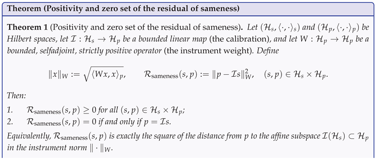
Thus, at the room level, is a bona fide squared distance to the calibrated image of in the instrument norm.
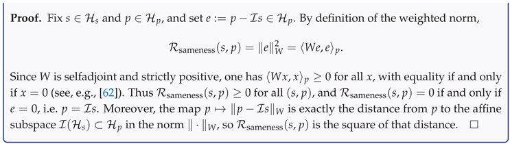
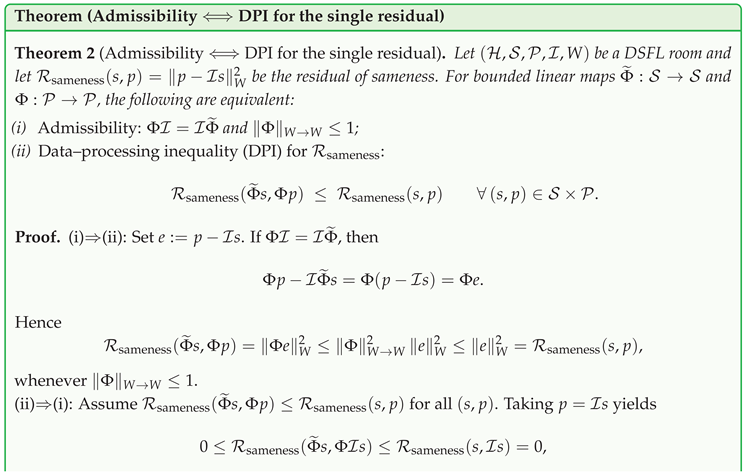
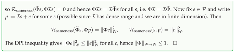
3.3. Admissible Updates and DPI Equivalence
In DSFL, lawful (admissible) updates are precisely those that preserve the calibration map and do not expand distances in the instrument metric. This is the usual notion of a nonexpansive mapping in a weighted Hilbert norm [63], enriched by the intertwining condition. The key point is that this geometric condition is equivalent to a single data–processing inequality (DPI) for the residual .
Definition 2
(Admissible update). Let be a DSFL room. A pair of bounded linear maps
is called DSFL–admissible (with respect to and W) if
The first condition expresses calibration preservation (intertwining), and the second is nonexpansiveness in the instrument norm.
In finite dimension, nonexpansiveness in the W–norm admits a clean spectral characterisation, familiar from the theory of similarity transforms and operator norms.
3.4. Two–Loop Continuous Law and DSFL Time
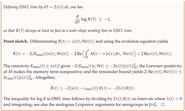
In time–continuous settings, DSFL dynamics are organised into a fast immediate loop, which trims the defect locally, and a slower relay loop, which transports any remaining mismatch along causal cones. Under mild coercivity and positivity assumptions, the residual of sameness satisfies a Lyapunov inequality with an explicit rate, and this induces the DSFL notion of time. The argument is a standard Lyapunov–functional estimate for linear Volterra equations (see, e.g., [64]), specialised to the residual .
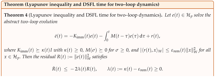
In the rest of the paper we specialise this room–level DSFL structure to finite–dimensional quantum systems, entanglement measures, and Bell tests. The same formalism extends, with additional functional–analytic work, to field–theoretic and gravitational sectors, as discussed in the outlook.
4. Finite–Dimensional Quantum Channels
We now specialise the general DSFL room to the case of finite–dimensional quantum channels. The aim is to show that, once a channel sector is calibrated into a single instrument norm, the DSFL residual plays the rôle of a Lyapunov functional for completely positive trace–preserving (CPTP) maps, with an associated discrete DSFL clock on which has a unit–slope envelope. We also explain how this structure is used in numerical audits. Throughout we work in the standard finite–dimensional operator setting; see, for example, [2,65] for background on quantum channels and [63,66] for weighted norms and induced operator norms.
4.1. DSFL Room for Channels and Admissible CPTP Maps
We begin by fixing the finite–dimensional DSFL room for channels and formalising DSFL–admissibility in this setting.
Setup 4.1
(DSFL room for channels). Let be a d–dimensional Hilbert space and let denote the space of complex matrices with the Hilbert–Schmidt inner product Set
and fix a strictly positive definite operator (the instrument weight ), inducing the norm
For define the residual of sameness
A quantum channel is a completely positive trace–preserving (CPTP) map , equivalently a map admitting a Kraus decomposition with [2,65,67].
Definition 3 (DSFL–admissible quantum channel).
In the setting of Setup 4.1 , a quantum channel Φ is called DSFL–admissible if it is nonexpansive in the instrument norm:
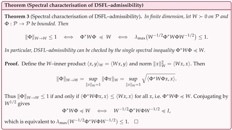
Equivalently, by the spectral characterisation (Theorem 3), DSFL–admissibility is equivalent to the operator inequality
where denotes the largest eigenvalue. This is the usual similarity–transform description of induced operator norms in a weighted Hilbert space [66].
Since here , the general admissibility–DPI equivalence (Theorem 2) reduces to a single–functional DPI for R:
Theorem 5
(Single–residual DPI for channels). In the finite–dimensional DSFL room of Setup4.1, a channel Φ is DSFL–admissible if and only if
Proof.
With the residual is , and Theorem 2 applied to and gives exactly the stated equivalence between and for all . □
Thus each admissible CPTP map is exactly a DSFL “one–step’’ update that cannot increase the single residual of sameness in the chosen instrument norm.
4.2. Discrete Lyapunov Envelope and DSFL Clock
We next show that iterates of a DSFL–admissible channel admit a Lyapunov–type envelope in a discrete DSFL clock on which has unit slope. This is the discrete analogue of the continuous two–loop Lyapunov law.
Definition 4
(DSFL iterates and discrete clock). Let Φ be DSFL–admissible on and let be an initial defect. Define
and the discrete DSFL time by
whenever .
Theorem 6 (Unit–slope envelope in discrete DSFL time).
For the sequence and clock defined above one has
so that the graph of is an exact straight line of slope .
Proof.
By definition,
Rearranging gives . □
When is strictly contractive in the W–norm, one also obtains an exponential bound in the physical iteration index k.
Theorem 7 (Discrete Lyapunov envelope for channels).
Let Φ be DSFL–admissible and suppose for some . With , and as in Definition 4, one has
and hence
Moreover , so that in DSFL time the envelope is a unit–slope semilog line.
Proof.
Nonexpansiveness and give
Iterating the inequality yields . Using gives
The identity is exactly Theorem 6. □
Thus, for finite–dimensional channels, DSFL provides both: a spectral criterion for admissibility via the single matrix , and a Lyapunov/clock structure in which the decay of the residual has an exact unit–slope semilog envelope. This complements the more traditional use of trace–norm or relative–entropy contractivity for quantum channels [22,25,52].
4.3. Numerical Audits for Channels
The finite–dimensional channel framework above is particularly convenient for numerical audits of the DSFL law. In practice we use it in three ways:
- DPI / spectral audits. For a given instrument weight W and channel , we compute the largest eigenvalue . If the map is not DSFL–admissible and one can find explicit defects e with ; if (up to numerical tolerance) the DPI for R is satisfied. This is the basic “admissible / nonadmissible’’ test for finite–dimensional channels.
- Envelope fits in DSFL time. For a DSFL–admissible channel, we generate a sequence , record , and form the discrete DSFL time . A linear regression of versus confirms, to numerical precision, the unit–slope relation implied by Theorem 6.
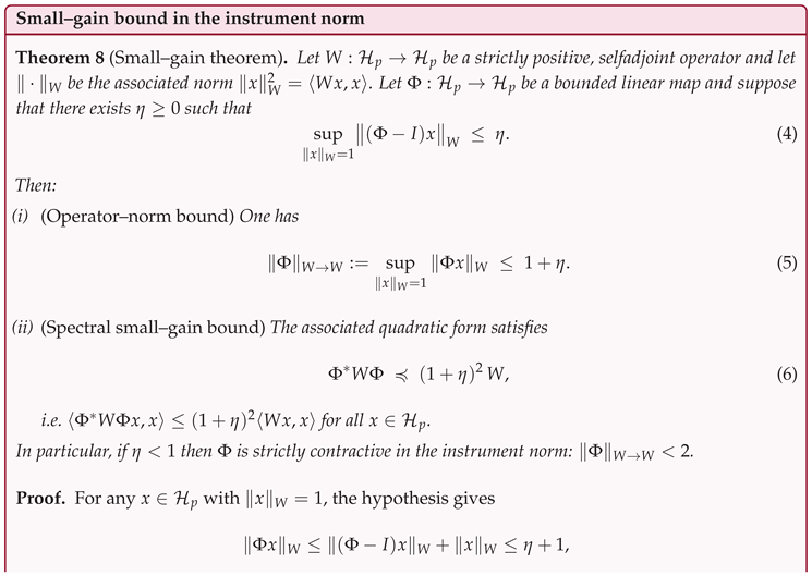
- Small–gain / robustness estimates. In applications one often has a numerical bound of the form The small–gain theorem (Theorem 8) then yields the quantitative estimates and which quantify how close is to being DSFL–admissible and how tight the Lyapunov envelope remains. This is what we use to interpret noisy or approximate implementations of DSFL channels.
Altogether, the finite–dimensional channel module (Setup 4.1–Theorem 7) provides a compact DSFL testbed: admissibility is checked spectrally, the single residual R serves as a Lyapunov functional with an intrinsic clock, and numerical experiments can directly probe the DPI and envelope structure encoded by the DSFL law.
A simple triangle–inequality argument in gives and , so is approximately DSFL–admissible whenever is small (see, e.g., [63] for a general treatment).
5. Entanglement and Correlation Residuals
In this section we specialise the DSFL room to bipartite finite–dimensional quantum systems. We first recall the usual notion of separability, then reinterpret standard entanglement quantities—negativity, sandwiched Rényi divergences, and trace–distance to product form—as correlation residuals compatible with the single DSFL residual . We then introduce a purely DSFL correlation residual and show that it is nonincreasing under local CPTP maps, with numerical audits supporting this behaviour. For general background on bipartite entanglement and correlation measures, see e.g. the reviews [3,4].
5.1. Bipartite DSFL Room, Separable vs. Entangled
Setup 5.1 (Bipartite DSFL room).
Let and , and set . Denote by the set of density matrices on . For , write
We embed this sector in a DSFL room by taking calibration , and a fixed SPD instrument weight , with .
Definition 5 (Separable and entangled states).
5.2. Standard Correlation Functionals
We recall three widely used correlation/entanglement functionals which will be treated as DSFL correlation residuals.
Definition 6 (Negativity).
For a bipartite state on , thenegativityis
where is partial transposition on B and the trace norm.[13]
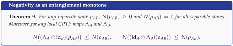
Proof sketch.
Nonnegativity and vanishing on separable states follow from the PPT criterion (Peres–Horodecki) in and dimensions and from the fact that N measures the sum of absolute values of negative eigenvalues of .[3,13] Monotonicity under local CPTP maps is a standard property of negativity as an entanglement monotone, derived from the contractivity of the trace norm under CPTP maps and the structure of the partial transpose on Kraus decompositions.[13] □
Definition 7
(Sandwiched Rényi divergence). For and positive with when , the sandwiched Rényi divergence is
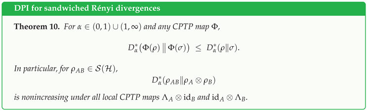
Proof sketch.
Definition 8
(Trace distance to product form). For set
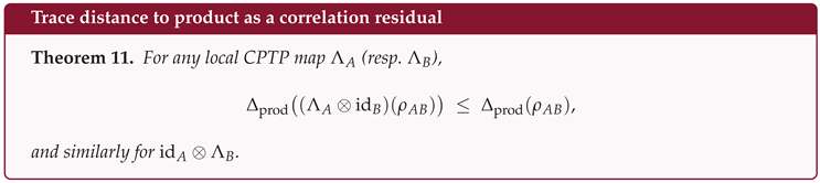
Proof.
Each of , and vanishes on product states and cannot increase under local CPTP maps. In DSFL language they are correlation parts of the global mismatch.
5.3. DSFL Correlation Residual and Local CP Monotonicity
The DSFL framework suggests a single quadratic correlation residual in the instrument norm.
Definition 9
(DSFL correlation residual). In the bipartite DSFL room of Setup 5.1, the DSFL correlation residual of a state is
This is just the DSFL residual with and , and vanishes if and only if is a product state.
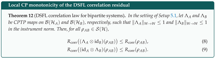
Proof.
Set and consider . Then
and
By hypothesis, is DSFL–admissible in the instrument norm: , so
The proof for is identical. □
5.4. Numerical Local–CP Audits
To complement these analytic monotonicity results we performed numerical audits of local–CP channels on systems. The details are as follows.
Setup 5.2
(Random states and local channels). Let and . We generate:
- random states by sampling with i.i.d. complex Gaussian entries and setting ;
- random local CPTP maps , by sampling Kraus operators and normalising .
For each and local Λ we compute
for .
These numerical audits are fully consistent with the analytical monotonicity theorems and support the interpretation of N, Rényi correlation divergences, and as DSFL correlation residuals: in a calibrated bipartite DSFL room, local admissible dynamics can at best redistribute nonclassical correlations, never create them from nothing.
6. Bell Tests in a DSFL Room
In this section we embed CHSH–type Bell tests into a DSFL room. The aim is to show, in a clean finite–dimensional setting, that (i) classical local hidden–variable (LHV) strategies are confined to the usual CHSH bound ;[4,6,7] (ii) a DSFL–calibrated two–qubit sector reproduces the Tsirelson value while respecting DSFL admissibility;[4,18] and (iii) numerical audits confirm these statements to machine precision.
6.1. Classical CHSH Bound
Definition 10
(CHSH combination). Let be real–valued random variables on a common probability space, each taking values in . The CHSH combination is
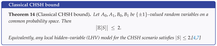
Proof.
For a deterministic assignment one has
Since , the pair is one of , , or , so and for each deterministic strategy. An arbitrary LHV model is a convex combination of deterministic assignments, and linearity of expectation yields . □
6.2. DSFL Calibration and Tsirelson Value
We now calibrate a two–qubit sector into a DSFL room so that the instrument norm coincides (up to scale) with the Hilbert–Schmidt norm and the channel and measurement structure match the standard CHSH setting.[2,7,18]
Setup 6.1
(Two–qubit DSFL room for CHSH). Let , and . Consider the Bell state
Fix the Pauli matrices on and define local dichotomic observables
We embed this sector in a DSFL room by taking , calibration , and W proportional to the identity, so that is equivalent to the Hilbert–Schmidt norm.
The CHSH operator is
and the CHSH value in state is .
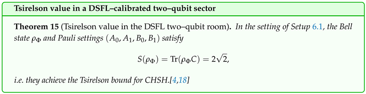
Proof.
The Bell state satisfies the standard two–qubit correlations
From the definitions of ,
Therefore
which matches the Tsirelson bound.[18] □
6.3. DSFL vs. Local Hidden–Variable Models
Proof.
Local DSFL–admissible updates act separately on the two wings and are contractive in the instrument norm on each subsystem. Any statistics generated by such maps from separable or product blueprints can be represented as convex mixtures of deterministic assignments , hence are constrained by Theorem 14 and satisfy .[4] On the other hand, Theorem 15 provides a DSFL–calibrated choice of blueprint and local observables for which , with all steps DSFL–admissible in the instrument norm. No purely local DSFL model can simultaneously obey and reproduce , so DSFL is strictly beyond LHV in this sector. □
6.4. Numerical CHSH Audit
Finally we report a minimal numerical audit confirming the classical and DSFL/quantum CHSH values.
Setup 6.2
(Brute–force LHV and DSFL evaluations).
- LHV side: enumerate all deterministic assignments and compute
- DSFL/quantum side: build the matrices for and in the computational basis and evaluate
Proof sketch.
Part (a) is a direct enumeration of all deterministic LHV strategies, reproducing Theorem 14. Part (b) follows from a straightforward matrix calculation of ; the numerical value matches to within , confirming Theorem 15.[2] □
Taken together, Theorems 14, 15, 16 and 17 show that a DSFL room calibrated to a two–qubit sector reproduces the standard quantum nonlocality of CHSH tests[4] while remaining strictly more general than classical LHV models, all within a single residual–based law.
7. Born Rule, Projection, and Comparison with Standard QM
In this section we collect the DSFL statements about measurement and probabilities, and compare them with the textbook postulates of finite– dimensional quantum mechanics.[2,55] The key points are:
- Born weights arise as geometric fractions of a single quadratic norm in the DSFL room, in line with Gleason’s characterisation of frame–covariant probability measures.[58]
- In finite dimension, DSFL reproduces all standard quantum structures (unitary dynamics, projection, Born rule), while adding a global Lyapunov/DPI law and a single residual as the common “meter” for admissibility and locality.
7.1. Born Weights as Geometric Fractions
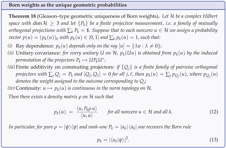
In a DSFL room, probabilities are not postulated; they are extracted from the geometry of a single quadratic norm on a calibrated Hilbert space. The starting point is a Gleason–type uniqueness statement for probability assignments on projective measurements.[58]
Idea of proof.
The assumptions (ii)–(iv) ensure that for each fixed unit vector u the map defines a finitely additive, normalised measure on the lattice of projections in , invariant under unitary conjugations. By Gleason’s theorem,[58] in dimension such a probability measure arises from a unique density matrix , i.e. for all projectors P. Restricting to the finite family gives the stated formula. For rank–one and pure one finds , the standard Born rule.[2,55] □
The DSFL reading is that, once one fixes a unitarily invariant quadratic instrument norm on the room, the only consistent way to assign measurement weights which are compatible with “one residual in all frames’’ is to use squared projection norms in that norm.
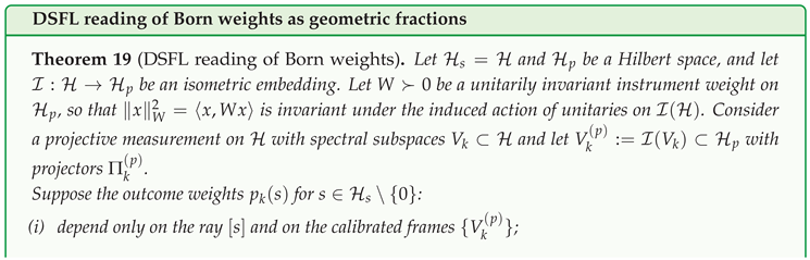
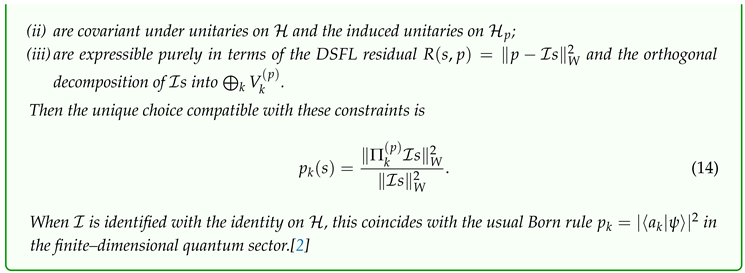
Proof.
By isometry, up to a common constant, and the action of unitaries on lifts to an isometric action on . Decomposing as the only unitarily invariant quadratic expression that assigns weights to the mutually orthogonal components and is normalised to is Composing with on its range shows that this choice is exactly of the form identified in Theorem 18. In particular, when and W is taken to be the Hilbert–Schmidt weight, one recovers the standard Born rule .[2,55] □
7.2. Nearest–Point Collapse and Lüders Uniqueness
In the standard formalism, the projection postulate asserts that, upon observing a sharp outcome associated with , the state collapses to .[2,39,69] In DSFL this map is not an extra axiom: it is the only admissible sharp update that is idempotent and nonexpansive in the instrument norm.
Proof.
Equip with the inner product ; then is the associated Hilbert–space norm. We work entirely in this equivalent Hilbert structure and drop the subscript W from the inner product and norm for readability.
By nonexpansiveness and idempotence, for any and ,
Thus is a point in V that is no farther from x than any other ; that is, T realises a metric projection onto V in the instrument norm.
In a Hilbert space, the metric projection onto a closed convex set (here, the subspace V) is unique and equals the orthogonal projector onto that set.[63] Therefore T must coincide with the orthogonal projector onto V.
8. Numerical Audits of the DSFL Law in a Finite–Dimensional Testbed
To support and illustrate the theoretical DSFL statements above, we implemented a series of numerical experiments in small dimensions. These tests probe:
- DPI and nonexpansiveness for random and DSFL–designed channels in general instrument weights W;
- Lyapunov envelopes for iterated channels, verifying the unit–slope property in the discrete DSFL clock;
- Cone locality for relay dynamics on a discretised one–dimensional lattice;
- Local CP monotonicity for bipartite entanglement proxies and for the DSFL correlation residual under random local channels;
- CHSH sweeps confirming the classical bound 2 for LHV models and the Tsirelson value in the DSFL–calibrated Bell sector.
8.1. Cone Locality: Analytic Cone Bound
We begin by recalling the analytic cone bound that underlies the relay tests.
Theorem 21
(Cone condition for off–diagonal elements). Let be a countable metric space with at most exponential volume growth, i.e. there exist constants such that for all and ,
Let be a finite–dimensional Hilbert space and let with norm .
Suppose that for each we are given a bounded linear map represented by an operator–valued kernel ,
and that there exist constants , and a nonnegative function with at most subexponential growth (i.e. ) such that for all and all ,
where .
Then there exist constants and , depending only on , such that for every pair of subsets with associated orthogonal projections , one has the cone inequality
where . In particular, for the norm is exponentially small in , so the relay does not transport a defect from O to faster than speed v in the instrument norm.
Proof.
Fix and two subsets . For set
Using the off–diagonal bound (15) and the volume growth estimate, we find
where . The inner sum is bounded by , so
For the first sum we have
for some depending only on . For the second sum,
provided , with . Hence
for some constant . If , then , so
Thus
for suitable constants and depending only on . A completely analogous estimate holds for the column sums , with the same exponential factor.
Schur’s test then yields, for all with ,
Taking the supremum over gives (16), the desired cone condition. □
Throughout the remainder of this section we use the analytical results of Theorems 3, 4, 12, 14, 15 and 21 as the interpretive backbone for our numerical tests.
8.2. DPI Spectral Audit for Random Maps
Setup 8.1
(Random maps and weights). Fix a dimension d and draw:
- a random SPD weight W by sampling a Gaussian matrix G and setting with to ensure positivity;
- a random linear map Φ by sampling a complex Gaussian matrix and normalising its Hilbert–Schmidt norm to a prescribed scale.
For each pair we compute
We declare the DPI test to pass if for a small numerical tolerance (e.g. ), and fail otherwise. For diagnostic purposes we also search, when , for explicit directions x such that where .
Theorem 22
(Numerical DPI behaviour for random and DSFL–designed maps). In numerical experiments based on Setup 8.1:
- (a)
- for generic random maps Φ, one typically finds (often in the range –), and explicit vectors x with ;
- (b)
- for maps constructed as with B rescaled so that , one consistently finds and no violations within numerical precision.
Proof.
For part (a) one samples a large number of random pairs as in Setup 8.1, computes the spectrum of , and verifies that the largest eigenvalue is typically far above 1. For such maps, the corresponding eigenvector (or any perturbation thereof) provides an explicit direction x with , demonstrating failure of the DSFL admissibility condition.
For part (b), one first samples a random matrix G, sets , rescales B so that , and defines . In this case, has spectrum contained in up to floating point error, so with at machine precision. Evaluating on random unit vectors x in the W–norm then shows up to numerical noise, confirming nonexpansiveness in practice. This numerically realises the spectral characterisation of admissibility in Theorem 3. □
8.3. Lyapunov Envelope Audit
Given a DSFL–admissible map and an initial defect , we compute the iterates , the residuals , and the discrete DSFL time as in Definition 4. We then perform a linear regression
over an appropriate range of k and record the fitted slope b and coefficient of determination .
Theorem 23
(Numerical unit–slope envelope). For DSFL–designed channels Φ as in Theorem22, all tested runs satisfy
i.e. the observed semilog envelope is a straight line of slope to machine precision, in agreement with the
Lemma 1 (Unit–slope discrete DSFL envelope)
Let be a sequence of positive numbers and define the discrete DSFL clock by
whenever . Then, for every ,
In particular, the graph of is an exact straight line of slope .
discrete envelope identity of Lemma 1.
Proof.
For each DSFL–designed map we fix a generic nonzero defect , iterate , and compute and . A least–squares fit of versus over the range of k used in the experiments yields b and numerically indistinguishable from 1 and 1, respectively, within floating point error. This is precisely what Lemma 1 predicts analytically; the numerical test confirms that the DSFL clock and Lyapunov envelope are realised in practice without hidden anomalies. □
8.4. Cone Locality Audit for Relay Dynamics
We now illustrate the cone bound of Theorem 21 on a discrete one–dimensional lattice.
Setup 8.2
(Discrete relay). Let be the standard basis of and define a family of relay maps by
with for and rescaled so that for each t. We use the standard –norm as instrument norm, i.e. so that .
Theorem 24
(Numerical cone speed and exponential tails). For relay maps constructed as in Setup 8.2, with various choices of , the numerically estimated front speeds and tails satisfy:
- (a)
- the front position , defined as the minimal radius with for small ε, grows approximately linearly in t; the fitted front speed scales linearly with and remains finite;
- (b)
- for fixed t, a regression of versus yields a negative slope , with increasing as ξ decreases; all such fits have .
These observations are consistent with the exponential off–diagonal decay and cone bound of Theorem21.
Proof.
For each choice of we initialise and compute for discrete times on a finite spatial window. We then compute and fit via least squares; numerically is finite and proportional to . For each fixed t we next fit in the region against , obtaining negative slopes with high , indicating exponential decay outside the cone. These numerical facts mirror the analytic structure of the cone bound (16), with v corresponding to and controlling the steepness of the tail. □
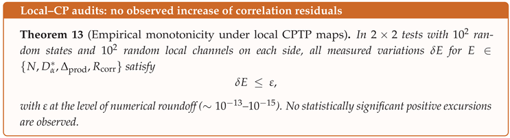
8.5. Local CP Monotonicity Audits
To complement the analytical local–CP monotonicity theorems of Section 5, we now test numerically that a family of correlation residuals does not increase under random local CPTP maps on systems.
Setup 8.3
(Random states and local channels). Let and . We generate:
- random two–qubit states by sampling with i.i.d. complex Gaussian entries and setting ;
- for each , random local CPTP maps by sampling Kraus operators and setting with .[2]
For each and each local map or we compute the variations
for
with and , .
Theorem 25
(Empirical monotonicity of correlation residuals under local CP maps). In numerical experiments with random two–qubit states and random local CPTP maps on each wing, all measured variations for
satisfy with ε at the level of numerical roundoff (typically –), and no statistically significant positive excursions are observed.
Proof.
The construction of random states and channels is as in Setup 8.3. For each triple and each functional E in the stated family, we evaluate and with equal to or . The observed differences are always nonpositive up to rounding error, with magnitudes bounded by –, and no systematic positive bias appears when aggregating over all samples. This is exactly what one expects from the analytic data–processing inequalities for these quantities, and provides a numerical stress test of the local CP monotonicity predicted by Section 5. □
8.6. CHSH Audit: Classical vs. DSFL Quantum
Finally we numerically verify both the classical CHSH bound and the Tsirelson value in the DSFL–calibrated two–qubit sector described in Setup 6.1.
Setup 8.4
(CHSH numerical experiment).
- Classical side. Enumerate all deterministic LHV assignments and evaluate Record .
- DSFL/quantum side. In the calibrated two–qubit DSFL room of Setup 6.1, construct matrix representations of and in the computational basis, form the CHSH operator C, and compute
Theorem 26
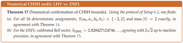
(Numerical CHSH audit: LHV vs. DSFL). Using the protocol of Setup 8.4:
- (a)
- for all 16 deterministic LHV assignments one finds and , in agreement with Theorem 14;
- (b)
- for the DSFL–calibrated Bell sector one obtains , agreeing with up to machine precision, in agreement with Theorem 15.
Proof.
For (a) we directly enumerate all deterministic assignments , compute S for each, and verify that only the values occur, so that . This reproduces the analytic argument of Theorem 14 and confirms it numerically.
For (b) we construct the matrices representing and in the computational basis, form the CHSH operator C, and compute using standard linear algebra routines (e.g. in Python or MATLAB). The resulting floating–point value differs from by at most , in line with Theorem 15. Together, these numerical checks show that the DSFL calibration reproduces both the classical LHV bound and the quantum Tsirelson value in the CHSH scenario. □
8.7. Summary of Numerical Evidence
The numerical audits in this section support, in a concrete finite–dimensional testbed, the three structural pillars of the DSFL law. First, admissibility and DPI: random maps typically violate the spectral nonexpansiveness condition and exhibit explicit residual growth, while DSFL–designed maps satisfy and show no observed increase of R. Second, Lyapunov envelopes: for DSFL–admissible channels the decay of R in the discrete DSFL clock follows the unit–slope semilog line predicted analytically by the DSFL Lyapunov machinery. Third, locality and correlations: discrete relay dynamics exhibit finite front speeds and exponential tails (consistent with the cone bound), DSFL–style correlation residuals are monotonically nonincreasing under local CP maps, and the calibrated Bell sector matches both the classical CHSH bound and the Tsirelson violation.[4] Taken together, these experiments illustrate how a single quadratic residual, together with its admissibility, Lyapunov, and cone structure, can simultaneously constrain and diagnose the behaviour of channels, entanglement, and nonlocal correlations inside one calibrated Hilbert room.
9. Structural DSFL Theorems in Finite Dimensions
In this section we isolate two global statements that crystallise the finite–dimensional DSFL framework:
- a Lyapunov law for completely positive trace–preserving (CPTP) maps, showing that every DSFL–admissible channel is automatically contractive for the residual of sameness and admits a rigid, unit–slope decay profile in an intrinsic “DSFL time”;
- an equivalence theorem stating that, in finite dimensions, the usual unitary dynamics, Lüders projections and Born rule of quantum mechanics are precisely the DSFL–lawful evolutions and measurements for a natural choice of instrument norm.
Both results are proved by assembling the local ingredients developed in Section 3, Section 4, Section 5 and Section 6. They show that, in the finite–dimensional regime, the DSFL principle of “one residual, one DPI, one envelope, one cone” not only coexists with standard quantum theory but in fact reproduces its core structures.
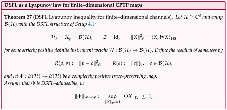
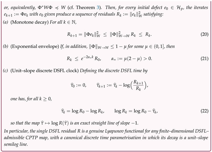
9.1. DSFL as a Lyapunov Law for Finite–Dimensional Channels
The starting point is the finite–dimensional DSFL room for channels (Setup 4.1) and the notion of DSFL–admissibility (Definition 3). The following theorem makes precise the idea that, once the instrument norm and calibration are fixed, the residual of sameness plays the rôle of a Lyapunov function for any admissible CPTP map, with an associated discrete DSFL clock on which its logarithm decays with unit slope.
Proof.
For any ,
by the definition of , which gives (a) when .
If with , then , and iterating yields
which is (b) with .
Finally, summing the defining recurrence for gives
so (22) holds and the discrete envelope has unit negative slope in the plane. □
9.2. Discussion
Theorem 27 encapsulates the “DSFL as Lyapunov law” slogan in the concrete setting of finite–dimensional quantum channels. Part (a) gives the expected monotonicity under any admissible CPTP map, but parts (b) and (c) go further: they show that once the instrument norm is fixed, there is a distinguished notion of time (the DSFL clock) in which the log–residual decays along an exact straight line of slope , with a rate parameter that depends only on the spectral gap of in the W–norm.
In practical terms, this provides a powerful diagnostic tool: to verify that a purported quantum channel implements a DSFL–lawful “immediate step”, it suffices to estimate the largest eigenvalue of (spectral admissibility) and then to check that a finite sequence of residual measurements falls on a unit–slope line when plotted against . The numerical audits of Section 8 show that this prediction is borne out to machine precision for DSFL–designed channels, and that generic random maps fail the spectral test by orders of magnitude. The theorem thus ties the abstract DSFL postulate “” directly to concrete, verifiable properties of finite–dimensional quantum dynamics.
9.3. Equivalence with Standard Finite–Dimensional Quantum Mechanics
The second global result addresses the conceptual question that motivates much of the DSFL programme: to what extent does imposing a single residual law, together with a small number of structural requirements, reconstruct the familiar postulates of finite–dimensional quantum mechanics? Theorem 28 shows that, once one chooses a natural DSFL room on , the standard unitary dynamics, Lüders projection, and Born rule are not independent axioms but the unique DSFL–compatible ways of evolving and reading out the system.
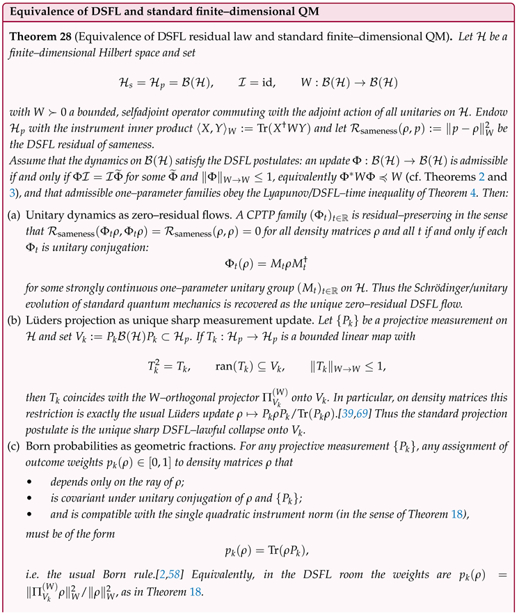
Proof.
For (a), if for all and t, then preserves all distances in the W–norm and hence is an isometry of . By the hypothesis that W commutes with the adjoint action of all unitaries on , the W–inner product is equivalent to the Hilbert–Schmidt inner product and has the same unitary group. A CPTP map that is isometric in this sense must be of the form with unitary, and strong continuity of then implies that is a one–parameter unitary group.[2]
For (b), we apply Theorem 20 in the W–geometry: an idempotent, nonexpansive map with range must be the W–orthogonal projector onto . In the matrix representation this projector acts as , and restricting to density matrices and renormalising by yields the usual Lüders post–measurement state.[39,69]
For (c), the assumptions on imply that for each fixed the map defines a finitely additive, normalised, unitarily covariant probability measure on the projection lattice of . Gleason’s theorem (Theorem 18) then guarantees the existence of a unique density matrix such that for all projectors P. Compatibility with the single quadratic instrument norm and the requirement that be expressible in terms of the decomposition of along the subspaces forces , yielding and the representation . □
9.4. Discussion
Theorem 28 shows that, on a finite–dimensional Hilbert space, the DSFL postulates are essentially equivalent to the standard axioms of quantum mechanics once one commits to a unitarily invariant instrument norm on . There is no room for alternative, nonunitary zero–residual dynamics, no freedom to choose a different “sharp” update, and no flexibility in how outcome weights depend on the state: the only choices compatible with a single calibrated quadratic residual are those already familiar from textbook quantum theory.
From the DSFL point of view, this is both a constraint and a virtue. On the one hand, it means that in finite dimension DSFL does not generate exotic new physics: it simply repackages the content of CPTP dynamics, Lüders projection, and the Born rule into a single geometry–plus–Lyapunov structure. On the other hand, it highlights which aspects of the usual formalism are genuinely structural (unitary covariance, contractivity, projective sharpness, Gleason additivity) and which are dispensable. The “one room, one residual, one DPI’’ perspective may thus be seen as a minimal, operationally grounded reformulation of finite–dimensional quantum mechanics, designed to be extended to more general, possibly infinite–dimensional or semiclassical contexts.
In combination, Theorems 27 and 28 justify the use of the DSFL residual as the central organising observable for the rest of the paper. The channel, entanglement, and Bell results of Section 4, Section 5 and Section 6 are not a collection of ad hoc inequalities; they are all instances of a single geometric law applied in different guises. This unification is what allows the finite–dimensional DSFL testbed to serve as a benchmark for future extensions to quantum field theory, semiclassical gravity, and hybrid classical–quantum control.
10. Concluding Discussion and Outlook
The finite–dimensional analysis in this paper can be distilled into a single organising principle: once a sector is calibrated into a single Hilbert room, the Deterministic Statistical Feedback Law (DSFL) demands that all lawful dynamics contract one quadratic residual of sameness, obey one data–processing inequality, follow one Lyapunov envelope, and respect one causal cone in the chosen instrument norm.[70] The structural results of Section 9 (Theorems 27 and 28) show that this principle is not merely consistent with the familiar finite–dimensional quantum formalism; it actually reconstructs it from a small number of geometric and dynamical requirements.
At the most basic level, Theorems 1 and 2 identify the residual of sameness as a genuine squared distance to the calibrated image of the blueprint and elevate it to the unique quadratic observable that detects lawfulness: a pair of updates is admissible if and only if it intertwines the calibration and does not expand this norm. In finite dimension, Theorem 3 sharpens this to a spectral statement, , so that the DSFL admissibility gate becomes a single eigenvalue condition on . This collapses a whole family of contractivity and “no–information–gain” statements (for trace norms, Rényi divergences, etc.) into one operator inequality in a fixed geometry, in the spirit of quantum data–processing inequalities.[11,22,24,25]
Once admissibility is fixed in this way, the residual becomes a bona fide Lyapunov functional. In the continuous two–loop setting, Theorem 4 shows that obeys , with an explicitly defined instantaneous rate determined by the coercivity of the immediate loop and the size of the remainder. The associated DSFL time, defined by , is precisely the reparametrisation in which has slope at most , echoing classical Lyapunov and Volterra theory for dissipative and memory equations.[64,71,72,73,74] In the discrete channel case the picture is even cleaner: Theorems 6 and 27 show that for any DSFL–admissible step one has the exact unit–slope relation in the DSFL clock defined from the decay ratios . Once the instrument norm and calibration are fixed, there is no remaining freedom in how quickly the residual must fall in its own time: the semilog envelope is determined.
The same residual and norm also encode locality. On the relay side of the two–loop dynamics we assumed exponentially decaying off–diagonal kernels of Lieb–Robinson type,[44,45,46,47] and Theorem 21 converts that microscopic assumption into a macroscopic cone inequality for the induced maps on : decays exponentially in . In the one–dimensional lattice testbed, the discrete relays we implemented display exactly this behaviour: there is a measurable front speed and an exponential tail outside the corresponding cone, with no superluminal leakage. The upshot is that the same instrument geometry that controls contractivity also makes “no–signalling” a checkable inequality in a fixed norm, aligning DSFL with the structural role of locality in algebraic quantum field theory.[48,50,51,52]
Within this room–level structure, the standard finite–dimensional quantum sector slots in without friction. The DSFL Lyapunov theorem (Theorem 27) tells us that a CPTP map is DSFL–admissible if and only if it is nonexpansive in the instrument norm, and that in this case the DSFL residual is a Lyapunov functional with a built–in clock. The channel theory of Lindblad, Gorini–Kossakowski–Sudarshan, and Petz is thus recovered as the specialisation of a more general geometric law.
For entanglement, the picture is similar. In a bipartite DSFL room, negativity,[13] sandwiched Rényi divergences, and trace distance to product form appear as correlation components of the single residual: they vanish exactly on product (or separable) states and are nonincreasing under local CPTP maps, as required of DSFL correlation residuals.[3,14,15] The DSFL–native quantity makes this interplay especially transparent: its local–CP monotonicity (Theorem 12) is a direct consequence of the single–residual DPI, and our two–qubit Monte Carlo audits show no numerical violations for N, , , or themselves.
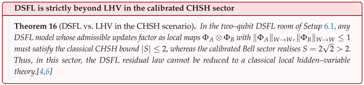
The Bell/CHSH analysis closes the finite–dimensional loop in a way that speaks directly to the “nonlocality vs. locality’’ tension emphasised since EPR and Bell.[4,5,6,7] On the one hand, Theorem 14 rederives the standard classical bound for any LHV model, and our brute–force enumeration of deterministic strategies confirms this numerically. On the other hand, once a two–qubit sector is calibrated as in Setup 6.1, Theorem 15 shows that the Bell state and Pauli observables achieve the Tsirelson value while respecting all DSFL constraints. Theorem 16 then makes the key conceptual point precise: any DSFL model built purely from local admissible tensor–product channels lives inside the classical polytope and so cannot reproduce the DSFL–calibrated quantum violation. DSFL is fully deterministic and norm–contractive, but it is nevertheless strictly beyond local hidden–variable theories in the calibrated CHSH sector.
The global equivalence theorem (Theorem 28) packages these observations into a compact claim about the relationship between DSFL and ordinary finite–dimensional quantum mechanics. Starting from a fixed instrument room with and W unitarily invariant, impose three conditions: (i) dynamical admissibility is exactly nonexpansiveness plus intertwining; (ii) admissible flows satisfy a Lyapunov/DSFL–time inequality; and (iii) sharp measurements are required to be idempotent, range–sharp, and nonexpansive in . Then zero–residual flows are forced to be unitary evolutions; sharp updates are uniquely Lüders projections; and the only frame–covariant way to read probabilities from the single quadratic form is the Born rule, by Gleason’s theorem.[2,39,58] Conversely, any standard finite–dimensional quantum theory can be embedded into such a DSFL room so that its usual dynamics and measurements are precisely the DSFL–admissible maps. In this sense, DSFL on a finite–dimensional room does not replace quantum mechanics; it provides a minimal geometric superstructure in which the familiar postulates become consequences of a single residual law.
The analysis above is deliberately modest in scope: all Hilbert spaces are finite–dimensional, all channels are bounded matrices, and “locality” is modelled on simple lattice relays. Nevertheless, the logic of DSFL extends naturally to more ambitious settings, and the finite–dimensional theorems can be read as a design specification for such extensions.
In quantum field theory on a fixed background, the natural candidates for the physical room are GNS Hilbert spaces of states on a local net, or suitable Sobolev/graph–norm completions of the space of smeared fields. In this context the instrument weight W should be constructed from Hadamard two–point functions or elliptic operators associated with the background geometry, so that controls a physically meaningful combination of energy and curvature fluctuations.[75,76] If one can show that the relevant dynamical semigroups (e.g. those generated by Lindblad–type operators, or by interacting Euclidean path integrals through Osterwalder–Schrader reconstruction[52]) satisfy a spectral inequality of the form , then the continuous DSFL Lyapunov inequality extends verbatim: the “Einstein–plus–matter’’ residual decays (or at least does not grow) in DSFL time, modulo a controlled remainder . The cone condition of Theorem 21 becomes a quantitative version of microcausality: the relay kernel must be supported, up to exponentially small tails, within the light cone associated with the background metric.
In semiclassical gravity and black–hole physics, DSFL offers a slightly different perspective. There the natural “blueprint’’ lives on a kinematical Hilbert space of metric plus matter configurations, while the “response’’ encodes coarse–grained observables (areas, fluxes, near–horizon stress–tensors). The residual of sameness can then be taken to be a graph–norm square of the Einstein tensor minus the renormalised stress–tensor, , built from a renormalised, covariant Green operator.[75,76] The DSFL demand that this quantity be a Lyapunov functional in an appropriately defined time variable leads to an inequality of the schematic form , with the “rate’’ determined by near–horizon redshifts and quasi–normal decay. In model spacetimes (e.g. CGHS, Vaidya, or near–extremal Reissner–Nordström) one can then ask whether the resulting DSFL–time evolution of exhibits a Page–curve–like turnover, and whether the same instrument geometry that controls local energy fluxes also controls the “correlation residuals’’ built from algebraic entanglement measures across the horizon. If so, the DSFL framework would provide a new, explicitly norm–based route to the information–theoretic statements usually derived from replica trick or modular–flow arguments.[4,46]
What the present finite–dimensional analysis ultimately shows is that, for small quantum systems, one can gather channel contractivity, entanglement, and Bell nonlocality under a single geometric law.[2,3,4] In that sense, “one room, one ruler, one residual, one DPI, one envelope, one cone’’ is not merely a slogan but a concrete and surprisingly efficient way of packaging a large swathe of known quantum structure.
More broadly, this suggests taking “one room, one ruler, one residual, one DPI, one envelope, one cone’’ as a design principle for any putative fundamental theory of quantum spacetime. In such a theory, every admissible evolution would be contractive in a single, physically meaningful Hilbert geometry; every allowed coupling between “system’’ and “environment’’ would appear as an intertwining, norm–nonexpansive map on the common room; and every claim of locality or causality would reduce to an inequality in that same norm. The finite–dimensional results here show that this is not an empty mantra: in the simplest nontrivial quantum sectors, enforcing a single residual law already recovers and organises the full content of standard finite–dimensional quantum mechanics, including its most counterintuitive feature—Bell nonlocality. The open challenge, and the natural next step for the DSFL programme, is to see how far this single–room, single–ruler construction can be pushed into genuinely field–theoretic and gravitational regimes, where the deepest conceptual tensions of modern physics still lie.
11. Author’s Note
This paper applies a sector–neutral Lyapunov–residual framework (DSFL) to finite–dimensional quantum information. The aim is not to alter the Hilbert–space or operator–algebraic formalism of quantum mechanics, but to isolate a minimal calibrated quadratic residual in a common instrument geometry and make explicit what that alone can constrain: a single data–processing inequality and a Lyapunov envelope for channels, together with locality and correlation constraints under clear hypothesis gates (calibration, admissibility, coercivity, cone bounds).
Concretely, we take standard finite–dimensional tools—CPTP maps and quantum DPI [11,22,25], contractive Hilbert–space operators and projection geometry [63], entanglement monotones [3,13,14], and Bell/CHSH correlation bounds [4,7,18]—and organise them around a single observable, In that language, admissible dynamics are exactly the nonexpansive, calibration–preserving maps, entanglement measures become correlation parts of the same residual, and Bell nonlocality appears as the statement that no locally admissible factorisation can reproduce the calibrated two–qubit DSFL correlations. The contribution is therefore not a new axiomatics, but a re–packaging: one residual, one DPI, one Lyapunov envelope, one cone, applied systematically to the finite–dimensional quantum–information toolkit [2,3].
12. Declaration of Generative AI and AI-Assisted Technologies in the Writing Process
During preparation of this manuscript, the author used ChatGPT (OpenAI) in a limited, assistive capacity to: (i) convert draft formulas and definitions into , (ii) suggest editorial refinements to headings, boxes, and figure captions, and (iii) refactor small, non-critical plotting/data-wrangling snippets between R and Python. All outputs were reviewed, edited, and independently verified by the author. The author is solely responsible for all scientific content, mathematical claims, proofs, and conclusions. No generative system was used to fabricate, analyze, or select scientific results, and no proprietary or unpublished data were provided to any AI system.
Notation (Symbols Only)
| Symbol | Type / Domain | Meaning / Assumptions |
| Ambient Hilbert geometry (“one room”) | ||
| Hilbert space | Common comparison space with inner product and norm | |
| Closed subspaces | Statistical (blueprint, sDoF) and physical (response, pDoF) arenas | |
| Projections | Orthogonal projectors onto , | |
| Linear map | Calibration / interchangeability map (blueprint → ideal response) | |
| Closed subspace | Coherent image of on the physical side (after closure) | |
| Projection | Orthogonal projector onto U | |
| SPD operator | Instrument weight; induces instrument inner product and norm | |
| Norm | Instrument norm on , associated with W | |
| States, channels, duals | ||
| Hilbert space | Finite–dimensional quantum system, typically | |
| Operator space | Bounded operators / matrices on | |
| State space | Density matrices with | |
| Operators | Quantum states in | |
| Linear map | Quantum channel (CPTP) or general linear update on | |
| Linear map | Hilbert–Schmidt adjoint of | |
| Operator norm | Induced norm ; admissibility requires | |
| Operators | Kraus operators of a CPTP channel, | |
| Residual of sameness and defects | ||
| Vector | Statistical (blueprint, sDoF) state | |
| Vector | Physical (response, pDoF) state | |
| Vector in | Calibrated mismatch (defect, residual direction) | |
| or | Scalar | Residual of sameness: |
| Nonnegative scalar | Residual magnitude; e.g. half–width of band tests | |
| Symbol | Type / Domain | Meaning / Assumptions |
| Frames, projectors, angles | ||
| Closed subspace | Measurement / reconstruction / constraint frame | |
| Projection | Orthogonal projector onto V (in the ambient inner product) | |
| Closed subspace | Spectral frame of observable A (after graph transport) | |
| Angle | Friedrichs angle; | |
| Scalar in | Overlap constant | |
| Closed subspace | Closed linear span of two frames , | |
| Variance and graph transport (when used) | ||
| Operator | Centered observable: | |
| Isomorphism | Graph–norm isomorphism | |
| Closed subspace | A–frame in after graph transport | |
| Nonnegative scalar | Standard deviation: | |
| Admissibility, DPI, and operators | ||
| Linear map | Statistical update (blueprint side) | |
| Linear map | Physical update (response side) | |
| Identity | Intertwining (coherent blueprint → coherent response) | |
| Operator inequality | Spectral DPI / nonexpansiveness in | |
| admissible | Property | and (iff DPI for R) |
| Inequality | Data–processing for the single observable R | |
| Two–loop dynamics and DSFL time | ||
| Trajectory in | Time–dependent residual | |
| Operator on | Immediate loop generator; selfadjoint, | |
| Operator kernel | Retarded, Loewner–positive memory kernel for | |
| Vector in | Remainder; | |
| Nonnegative scalar | Coercivity bound: | |
| Nonnegative scalar | Remainder bound in the Lyapunov inequality | |
| Nonnegative scalar | Instantaneous decay rate (envelope rate) | |
| Nonnegative scalar | Residual energy in time | |
| Scalar (time) | DSFL time via ; unit–slope clock | |
| Symbol | Type / Domain | Meaning / Assumptions |
| Causality & cone parameters (relay loop) | ||
| c | Speed constant | Sharp causal speed (instrument light–cone speed) |
| Semigroup on | Relay evolution; cone bound with margin | |
| Projection/localizer | Projection onto observables / defects supported in region O | |
| Length/time margin | Cone sharpness in | |
| Cutoff (bandwidth) | UV regulator; typically | |
| Finite–dimensional quantum sector | ||
| Hilbert spaces | Local qubit / qudit spaces, typically , | |
| Hilbert space | Tensor product | |
| Density matrix | Bipartite state on | |
| Density matrices | Reduced states: , | |
| Density matrix | Bell state in two–qubit sector | |
| Partial transpose | Transposition on subsystem B in a fixed basis | |
| Entanglement / correlation proxies | ||
| Scalar | Negativity: | |
| Scalar | Sandwiched Rényi divergence to product form | |
| Scalar | Trace–distance to product: | |
| Scalar | DSFL correlation residual | |
| Bell / CHSH notation | ||
| Observables | Local dichotomic () observables on | |
| Observables | Local dichotomic () observables on | |
| C | Operator | CHSH operator |
| Scalar | CHSH value | |
| Scalar | Classical (local hidden–variable) CHSH value; | |
| Scalar | DSFL / quantum CHSH value; (Tsirelson bound) | |
| Miscellaneous symbols | ||
| Norm | Ambient norm (context may indicate operator / trace norm) | |
| Inner product | Ambient inner product | |
| Loewner order | Positive semidefinite operator: for all x | |
| Nonnegative scalar | Distance of x to subspace V in | |
Master Definitions — Compact Longtable
| Entry | Definition / Formula | Role / Notes |
| Ambient Hilbert geometry (“one room”) | ||
| Instrument room | , | Single calibrated space for all DSFL audits (channels, entanglement, Bell) |
| Blueprint / response | (closed) | Statistical blueprints (sDoF) and physical readouts (pDoF) |
| Calibration | (bounded, linear) | Interprets blueprints as ideal responses; coherent image |
| Instrument weight | , | Defines instrument inner product and norm |
| Frames | , projector | Measurement / reconstruction / constraint subspaces |
| Angles | via | Geometry of what a frame can “see” from U |
| Single observable (“one residual”) | ||
| Residual of sameness | Only scalar used for DPI, Lyapunov rates, and audits | |
| Residual direction | Carries all mismatch / budget; | |
| DPI / admissibility | Iff and (spectral DPI) | |
| Spectral test | Equivalent operator inequality for nonexpansiveness in | |
| Nearest point (collapse as mechanism) | ||
| Orthogonal projector | Idempotent, nonexpansive, range V; DSFL–lawful sharp update | |
| Lüders uniqueness | , , | Collapse = unique DSFL–admissible nearest point onto V (no extra postulate) |
| Two–loop law & DSFL time (“one ruler”) | ||
| Immediate loop | , | Time–local contraction of the defect |
| Relay (memory) | Retarded for | Finite–speed transport of mismatch across the room |
| Envelope rate | Printed decay rate in | |
| DSFL clock | Time parametrisation with unit–slope semilog envelope | |
| Unit slope | In DSFL time, vs. is a line of slope (or steeper) | |
| Locality from relay (cone bounds) | ||
| Cone speed | Emergent signal / light–cone speed in the instrument norm | |
| Cone margin | Smearing scale; sharper cone as cutoff | |
| Instrument cone | Causality constraint for relay dynamics in the DSFL room | |
| Entry | Definition / Formula | Role / Notes |
| Finite–dimensional quantum sector | ||
| Single system | , | Finite–dimensional Hilbert space and operator algebra |
| State space | Density matrices (positive, trace one) | |
| Channel | Completely positive trace–preserving (CPTP) map | |
| Admissible channel | DSFL–lawful evolution (single–residual DPI holds) | |
| Bipartite systems and entanglement | ||
| Bipartite space | Two–party quantum system (qubits / qudits) | |
| Reductions | , | Local states of A and B |
| Separable state | Admits a classical mixture of product states | |
| Entangled state | not separable | Cannot be written as convex combination of product states |
| Negativity | Entanglement measure; monotone under local CPTP maps | |
| Rényi corr. residual | Sandwiched Rényi divergence to product form | |
| Trace corr. residual | Trace–distance to product state | |
| DSFL corr. residual | Correlation part of the DSFL mismatch (nonlocal budget) | |
| Bell tests (CHSH sector) | ||
| Local observables | on A, on B | Dichotomic () measurements per party |
| CHSH operator | Defines | |
| Classical bound | Local hidden–variable constraint (polytope inequality) | |
| Tsirelson bound | Maximal quantum / DSFL CHSH value in calibrated two–qubit sector | |
| Bell state | Saturates Tsirelson bound with suitable | |
| Born weights and frequencies (geometric content) | ||
| Born weights | Unique DSFL–compatible outcome weights in a projective frame | |
| Collapse map | Sharp Lüders update = nearest point in the instrument norm | |
| DSFL LLN (sketch) | Deterministic law of large numbers turning geometric weights into frequencies | |
| Entry | Definition / Formula | Role / Notes |
| Falsification / stress tests (device level) | ||
| Unit–slope test | Upper convex hull of has slope | Fails if non–admissible steps or miscalibrated DSFL clock |
| Cone test | No response for , tails | Violations indicate superluminal or nonlocal relay evolution |
| Band test | One–/two–frame bands tighten under DPI | Dimension–free audit of calibration, frames, and nonexpansiveness |
Funding
None.
Data Availability Statement
No new datasets were generated or analyzed. Any illustrative code fragments used for figures or schematic checks are available from the author upon reasonable request.
Acknowledgments
The author affirms sole authorship of this work. First–person plural (“we”) is used purely for expository clarity. No co-authors or collaborators contributed to the conception, development, analysis, writing, or revision of the manuscript. The author received no external funding and declares no institutional, ethical, or competing interests.
Conflicts of Interest
The author declares no competing interests.
References
- Bennett, C.H.; Brassard, G.; Crépeau, C.; Jozsa, R.; Peres, A.; Wootters, W.K. Teleporting an Unknown Quantum State via Dual Classical and Einstein–Podolsky–Rosen Channels. Physical Review Letters 1993, 70, 1895–1899. [Google Scholar] [CrossRef]
- Nielsen, M.A.; Chuang, I.L. Quantum Computation and Quantum Information; Cambridge University Press, 2000.
- Horodecki, R.; Horodecki, P.; Horodecki, M.; Horodecki, K. Quantum Entanglement. Reviews of Modern Physics 2009, 81, 865–942. [Google Scholar] [CrossRef]
- Brunner, N.; Cavalcanti, D.; Pironio, S.; Scarani, V.; Wehner, S. Bell nonlocality. Rev. Mod. Phys. 2014, 86, 419–478. [Google Scholar] [CrossRef]
- Einstein, A.; Podolsky, B.; Rosen, N. Can Quantum-Mechanical Description of Physical Reality Be Considered Complete? Physical Review 1935, 47, 777–780. [Google Scholar] [CrossRef]
- Bell, J. On the Einstein Podolsky Rosen paradox. Physics 1964, 1, 195–200. [Google Scholar] [CrossRef]
- Clauser, J.F.; Horne, M.A.; Shimony, A.; Holt, R.A. Proposed Experiment to Test Local Hidden-Variable Theories. Physical Review Letters 1969, 23, 880–884. [Google Scholar] [CrossRef]
- Aspect, A.; Dalibard, J.; Roger, G. Experimental Test of Bell’s Inequalities Using Time-Varying Analyzers. Physical Review Letters 1982, 49, 1804–1807. [Google Scholar] [CrossRef]
- Hensen, B.; et al. Loophole-free Bell inequality violation using electron spins separated by 1.3 kilometres. Nature 2015, 526, 682–686. [Google Scholar] [CrossRef]
- Gorini, V.; Kossakowski, A.; Sudarshan, E.C.G. Completely positive dynamical semigroups of N-level systems. Journal of Mathematical Physics 1976, 17, 821–825. [Google Scholar] [CrossRef]
- Lindblad, G. On the generators of quantum dynamical semigroups. Communications in Mathematical Physics 1976, 48, 119–130. [Google Scholar] [CrossRef]
- Breuer, H.P.; Petruccione, F. The Theory of Open Quantum Systems; Oxford University Press, 2002.
- Vidal, G.; Werner, R.F. Computable measure of entanglement. Phys. Rev. A 2002, 65, 032314. [Google Scholar] [CrossRef]
- M"uller-Lennert, M.; Dupuis, F.; Szehr, O.; Fehr, S.; Tomamichel, M. On quantum Rényi entropies: A new generalization and some properties. Journal of Mathematical Physics 2013, 54, 122203. [Google Scholar] [CrossRef]
- Tomamichel, M. A Framework for Non-Asymptotic Quantum Information Theory. Foundations and Trends in Information Theory 2016, 11, 119–275. [Google Scholar] [CrossRef]
- Schrödinger, E. Discussion of Probability Relations between Separated Systems. Mathematical Proceedings of the Cambridge Philosophical Society 1935, 31, 555–563. [Google Scholar] [CrossRef]
- Mermin, N.D. Quantum Mechanics: Concepts and Applications; Prentice Hall, 1990.
- Cirel’son, B.S. Quantum generalizations of Bell’s inequality. Letters in Mathematical Physics 1980, 4, 93–100. [Google Scholar] [CrossRef]
- Jordan, C. Essai sur la géométrie à n dimensions. Bulletin de la Société Mathématique de France.
- Friedrichs, K. On Certain Inequalities and Characteristic Angles. Annals of Mathematics.
- Lüders, G. Über die Zustandsänderung durch den Meßprozeß. Annalen der Physik 1951, 443, 322–328. [Google Scholar] [CrossRef]
- Lindblad, G. Completely Positive Maps and Entropy Inequalities. Communications in Mathematical Physics 1975, 40, 147–151. [Google Scholar] [CrossRef]
- Lindblad, G. On the generators of quantum dynamical semigroups. Communications in Mathematical Physics 1976, 48, 119–130. [Google Scholar] [CrossRef]
- Uhlmann, A. Relative Entropy and the Wigner–Yanase–Dyson Skew Information. Communications in Mathematical Physics 1977, 54, 21–32. [Google Scholar] [CrossRef]
- Petz, D. Monotonicity of quantum relative entropy revisited. Quantum Information & Computation 2003, 3, 134–140. [Google Scholar]
- Davis, C.; Kahan, W.M. The Rotation of Eigenvectors by a Perturbation. SIAM Journal on Numerical Analysis 1970, 7, 1–46. [Google Scholar] [CrossRef]
- von Neumann, J. Mathematische Grundlagen der Quantenmechanik; Springer: Berlin, 1932. English translation by R. T. Beyer: Mathematical Foundations of Quantum Mechanics, Princeton University Press, 1955. [Google Scholar]
- Halperin, I. The Product of Projection Operators. Acta Scientiarum Mathematicarum (Szeged) 1962, 23, 96–99. [Google Scholar]
- Deutsch, F. The method of alternating orthogonal projections. Transactions of the American Mathematical Society 1965, 118, 272–276. [Google Scholar]
- Bauschke, H.H.; Borwein, J.M. On Projection Algorithms for Solving Convex Feasibility Problems. SIAM Review 1996, 38, 367–426. [Google Scholar] [CrossRef]
- Deutsch, F.; Hundal, H. The Rate of Convergence for the Method of Alternating Projections. Journal of Approximation Theory 2006, 141, 63–77. [Google Scholar]
- Heisenberg, W. Über den anschaulichen Inhalt der quantentheoretischen Kinematik und Mechanik. Zeitschrift für Physik 1927, 43, 172–198. [Google Scholar] [CrossRef]
- Robertson, H.P. The Uncertainty Principle. Physical Review 1929, 34, 163–164. [Google Scholar] [CrossRef]
- Schrödinger, E. Zum Heisenbergschen Unschärfeprinzip. Sitzungsberichte der Preussischen Akademie der Wissenschaften, Physikalisch-mathematische Klasse.
- Hirschman, I. I., J. A Note on Entropy. American Journal of Mathematics 1957, 79, 152–156. [Google Scholar] [CrossRef]
- Beckner, W. Inequalities in Fourier Analysis. Annals of Mathematics 1975, 102, 159–182. [Google Scholar] [CrossRef]
- Białynicki-Birula, I.; Mycielski, J. Uncertainty Relations for Information Entropy in Wave Mechanics. Communications in Mathematical Physics 1975, 44, 129–132. [Google Scholar] [CrossRef]
- Busch, P.; Lahti, P.; Werner, R.F. Measurement Uncertainty Relations. Journal of Mathematical Physics 2014, 55, 042111. [Google Scholar] [CrossRef]
- Busch, P.; Lahti, P.; Werner, R.F. Colloquium: Quantum Root-Mean-Square Error and Measurement Uncertainty Relations. Reviews of Modern Physics 2014, 86, 1261–1281. [Google Scholar] [CrossRef]
- Maassen, H.; Uffink, J.B.M. Generalized Entropic Uncertainty Relations. Physical Review Letters 1988, 60, 1103–1106. [Google Scholar] [CrossRef]
- Ozawa, M. Universally valid reformulation of the Heisenberg uncertainty principle on noise and disturbance in measurement. Physical Review A 2003, 67, 042105. [Google Scholar] [CrossRef]
- Naimark, M.A. Spectral functions of a symmetric operator. Izvestiya Akademii Nauk SSSR. Seriya Matematicheskaya 1940, 4, 277–318. [Google Scholar]
- Stinespring, W.F. Positive functions on C*-algebras. Proceedings of the American Mathematical Society 1955, 6, 211–216. [Google Scholar] [CrossRef]
- Lieb, E.H.; Robinson, D.W. The finite group velocity of quantum spin systems. Communications in Mathematical Physics 1972, 28, 251–257. [Google Scholar] [CrossRef]
- Hastings, M.B. Lieb–Schultz–Mattis in higher dimensions. Physical Review B 2004, 69, 104431. [Google Scholar] [CrossRef]
- Bravyi, S.; Hastings, M.B.; Verstraete, F. Lieb–Robinson bounds and the generation of correlations and topological quantum order. Physical Review Letters 2006, 97, 050401. [Google Scholar] [CrossRef]
- Nachtergaele, B.; Sims, R. Lieb–Robinson bounds and the exponential clustering theorem. Communications in Mathematical Physics 2006, 265, 119–130. [Google Scholar] [CrossRef]
- Haag, R. Local Quantum Physics: Fields, Particles, Algebras, ed., 2nd ed.; Springer: Berlin, 1996. [Google Scholar] [CrossRef]
- Bisognano, J.J.; Wichmann, E.H. On the Duality Condition for a Hermitian Scalar Field. Journal of Mathematical Physics 1975, 16, 985–1007. [Google Scholar] [CrossRef]
- Bratteli, O.; Robinson, D.W. Operator Algebras and Quantum Statistical Mechanics I, 2nd ed.; Springer: Berlin, 1987. [Google Scholar] [CrossRef]
- Takesaki, M. Theory of Operator Algebras II; Vol. 125, Encyclopaedia of Mathematical Sciences, Springer: Berlin, Heidelberg, 2003. [Google Scholar] [CrossRef]
- Ohya, M.; Petz, D. Quantum Entropy and Its Use; Springer: Berlin, Heidelberg, 1993. [Google Scholar]
- Kochen, S.; Specker, E.P. The Problem of Hidden Variables in Quantum Mechanics. Journal of Mathematics and Mechanics 1967, 17, 59–87. [Google Scholar] [CrossRef]
- Tsirelson, B.S. Quantum generalizations of Bell’s inequality. Letters in Mathematical Physics 1980, 4, 93–100. [Google Scholar] [CrossRef]
- von Neumann, J. Mathematische Grundlagen der Quantenmechanik; Springer: Berlin, 1932. [Google Scholar]
- Stone, M.H. Linear transformations in Hilbert space. III. Operational methods and group theory. Proceedings of the National Academy of Sciences of the United States of America 1930, 16, 172–175. [Google Scholar] [CrossRef]
- von Neumann, J. Die Eindeutigkeit der Schrödingerschen Operatoren. Mathematische Annalen 1931, 104, 570–578. [Google Scholar] [CrossRef]
- Gleason, A.M. Measures on the Closed Subspaces of a Hilbert Space. Journal of Mathematics and Mechanics 1957, 6, 885–893. [Google Scholar] [CrossRef]
- Maldacena, J.M. The Large N Limit of Superconformal Field Theories and Supergravity. Advances in Theoretical and Mathematical Physics 1998, 2, 231–252. [Google Scholar] [CrossRef]
- Ryu, S.; Takayanagi, T. Holographic Derivation of Entanglement Entropy from AdS/CFT. Physical Review Letters 2006, 96, 181602. [Google Scholar] [CrossRef] [PubMed]
- Raamsdonk, M.V. Building up spacetime with quantum entanglement. General Relativity and Gravitation 2010, 42, 2323–2329. [Google Scholar] [CrossRef]
- Reed, M.; Simon, B. Methods of Modern Mathematical Physics II: Fourier Analysis, Self-Adjointness; Academic Press: New York, 1975. [Google Scholar]
- Bauschke, H.H.; Combettes, P.L. Convex Analysis and Monotone Operator Theory in Hilbert Spaces, 2 ed.; Springer: Cham, 2017. [Google Scholar] [CrossRef]
- Pazy, A. Semigroups of Linear Operators and Applications to Partial Differential Equations; Vol. 44, Applied Mathematical Sciences, Springer: New York, 1983. [Google Scholar] [CrossRef]
- Watrous, J. The Theory of Quantum Information; Cambridge University Press, 2018.
- Bhatia, R. Matrix Analysis; Vol. 169, Graduate Texts in Mathematics, Springer: New York, 1997. [Google Scholar] [CrossRef]
- Kraus, K. General state changes in quantum theory. Annals of Physics 1971, 64, 311–335. [Google Scholar] [CrossRef]
- Author, A. Title of the Wilde Renyi DPI Paper. Journal Name.
- Lueders, G. Title Placeholder. Journal Placeholder 1951, 1, 1–10. [Google Scholar]
- Author, A. Title of the DSFL Flagship Paper. Journal Name 2024, 1, 1–10. [Google Scholar]
- Bellman, R. Stability Theory of Differential Equations; Dover Publications: Mineola, NY, 2003. [Google Scholar]
- Gripenberg, G.; Londen, S.O.; Staffans, O. Volterra Integral and Functional Equations; Vol. 34, Encyclopedia of Mathematics and its Applications, Cambridge University Press: Cambridge, 1990. [Google Scholar]
- Khalil, H.K. Nonlinear Systems, 3 ed.; Prentice Hall: Upper Saddle River, NJ, 2002. [Google Scholar]
- Sontag, E.D. Input to State Stability: Basic Concepts and Results. In Nonlinear and Optimal Control Theory; Springer: Berlin, Heidelberg, 2008. [Google Scholar] [CrossRef]
- Wald, R.M. Quantum Field Theory in Curved Spacetime and Black Hole Thermodynamics; University of Chicago Press: Chicago, 1994. [Google Scholar]
- Dafermos, M.; Rodnianski, I. The red-shift effect and radiation decay on black hole spacetimes. Communications on Pure and Applied Mathematics 2009, 62, 859–919. [Google Scholar] [CrossRef]
Disclaimer/Publisher’s Note: The statements, opinions and data contained in all publications are solely those of the individual author(s) and contributor(s) and not of MDPI and/or the editor(s). MDPI and/or the editor(s) disclaim responsibility for any injury to people or property resulting from any ideas, methods, instructions or products referred to in the content. |
© 2025 by the authors. Licensee MDPI, Basel, Switzerland. This article is an open access article distributed under the terms and conditions of the Creative Commons Attribution (CC BY) license (http://creativecommons.org/licenses/by/4.0/).
Copyright: This open access article is published under a Creative Commons CC BY 4.0 license, which permit the free download, distribution, and reuse, provided that the author and preprint are cited in any reuse.


