
Submitted:
14 November 2025
Posted:
17 November 2025
You are already at the latest version
Abstract
Subradiance is a phenomenon where coupled emitters radiate light at a slower rate than independent ones. While its observation was first reported in disordered cold atom clouds, ordered subwavelength arrays of emitters have emerged as promising platforms to design highly cooperative optical properties based on dipolar interactions. In this work we characterize the eigenmodes of 2D and 3D regular arrays, using a method which can be used for both infinite and very large systems. In particular, we show how finite-size effects impact the lifetimes of these large arrays. Our results may have interesting applications for quantum memories and topological effects in ordered atomic arrays.
Keywords:
superradiance
; subradiance
; cooperative emission
1. Introduction
Dicke superradiance corresponds to the enhancement of the radiation rate by N emitters due to coherence effects [1,2], as opposed to subradiance for which it is inhibited [3,4]. Recently, the subradiant suppression of radiative decay has spurred strong interest due to its potential applications for quantum memories [5,6], excitation transfer [7,8] and topological photonics [9]. Many-atom subradiance has been observed almost ten years ago in disordered clouds of cold atoms, with long lifetimes evidencing the phenomenon [10].
More recently, ordered sub-wavelength arrays of atoms have emerged as a promising configuration to achieve subradiance, with distinct advantages over disordered ensembles for applications such as photon storage or photonic gates [11,12,13,14,15,16]. In these systems, the emitters are regularly arranged with a spatial period below the atomic transition wavelength, so the dipolar interactions lead to strong cooperative optical properties.
In this context, infinite lattices offer interesting insights on the scattering properties of these arrays. The single-excitation eigenmodes of the scattering problem are translationally invariant and obey Bloch’s theorem. This allows one to define the quasi-momentum and calculate explicitly the collective frequency shift and decay rate of each of these modes [15]. Differently, in finite systems these collective features can only be accessed by numerical diagonalization, leading to severe limitations on the system size which can be simulated. Furthermore, most studies on subradiance in ordered systems have focused on one-dimensional (1D) atomic chains [6,7,8,17,18,19,20,21] and two-dimensional (2D) arrays [9,13,14,15,22], with investigations on the three-dimensional configurations lacking [23]. We note that while the band structure of 2D and 3D arrays have been studied through the density of states [24,25,26], the connection between this phenomenon and subradiance has not been yet clarified.
In this work, we investigate the cooperative decay rates of 2D and 3D atomic array, using a technique where the discrete sums over the emitters is turned into an angular integral. It provides the cooperative rate for the quasi-modes in infinite arrays [27]. But it is also particular convenient to study the rates of large size systems, for which the technique provides a good approximation, and numerical diagonalization are out of reach. Used successfully for 1D systems [27], we show the collective decay rates of the associated generalized Dicke state (also called generalized Bloch state [28]) can also be derived explicitly for 2D and 3D arrays. The work thus opens new perspectives for the study of cooperative scattering in large, regular atomic systems.
2. Microscopic Modeling of Atomic Arrays
2.1. Coupled Dipole Model
Let us consider N atoms with transition frequency between the ground state and the excited state (), linewidth , where ℏ is the Planck constant, the vacuum permittivity and the electric-dipole transition matrix element. The atoms are at fixed positions and have transition dipole moments , with . In the Born-Markov approximation, one can trace out the quantized light fields and obtain the field-mediated dipole-dipole couplings between the atoms described by an effective Hamiltonian [29]:
where is the lowering operator for atom j. The dyadic Green’s tensor for the electromagnetic field in the 3D free space in vacuum is given by
where is the identity tensor , and . The dyadic Green’s tensor (2) can be obtained from the scalar Green’s function [30]
If we assume that all transition dipoles point in the same direction, , such as in presence of a strong external field, the interaction term between atoms j and m read
with and . Note that has both a real and imaginary part, which describe the photon exchange between the atoms and their collective emission out of the system, respectively. Throughout this work we focus our attention on the imaginary part of , defining
Introducing the angular average
and using the property , we can rewrite as an angular average of the photon exchange term between the two atoms
where and . The remarkable property of Eq. (6) is that the contribution of the two atoms can now be factorized, which will allow us to calculate explicitly the collective decay rates, as we will later see.
2.2. Generalized Dicke State
We hereafter consider regular atomic arrays with lattice step d, with atoms at positions with , and , so is the total number of atoms. We then introduce the generalized Dicke states [27], or generalized Bloch states [28]:
The single-excitation states are and , where is the volume of first Brillouin zone in the reciprocal lattice, i.e., . It includes the symmetric Dicke state [1] for , as well as the timed-Dicke state introduced in Ref. [31,32] for a driving with wavevector . The family satisfies the completeness relation
For a finite lattice these states are not orthogonal since
nevertheless, in the limit of an infinite lattice the asymptotic property turns the set into an orthonormal basis for the single-excitation manifold.
2.3. Collective Decay Rate
The collective decay rate of mode is defined as [27]
Eq. (10) corresponds to the Fourier transform of only if the lattice is infinite, when modes (7) are the Bloch states and set is discrete. Nevertheless, treating as a continuous variable in Eq. (10) is a good approximation for the mode when N is sufficiently large [15]. We hereafter refer to as the “continuous spectrum” of the decay rate. We highlight that we are not referring to the discrete spectrum of the eigenvalues of the system, described by the non-Hermitian Hamiltonian (1), but rather to the imaginary part of the expectation value of the effective Hamiltonian on the collective state of Eq. (7), describing the interference among the (single-photon) fields emitted by N atoms. In particular, in the infinite N limit, is precisely the decay rate of mode , yet in the finite-N case, the exact rate must be obtained by diagonalizing the full matrix (1).
3. Two-Dimensional Square Lattice
3.1. General Expression of the Decay Rate
For a 2D atom array in the plane , with with and , the rate (11) reads
where the structure factor now factorizes for each direction:
Summing over and , we obtain
The property
can then be used, along with the assumption of large and , to write the decay rate as
where , , are the components of the reciprocal lattice vector . Note that different values of correspond to different Brillouin zones. In order to perform the integration over the angles and , we introduce the variables and , which leads to
We have here defined
so that . The final expression forthe rate then depends on the lattice size, , and we first discuss the case of an infinite 2D system.
3.2. Infinite Square Array
In the limit , using the property in the rate expression (18) leads to
with the condition , i.e., : Each term of the sums in Eq. (21) is different from zero inside a circle of radius and center in . This allows us to recover the result of Ref. [15] for parallel polarization, with the dipoles oriented in the array plane ():
as well as for perpendicular polarization, with the dipoles orthogonal to the 2D array plane ():
with the reciprocal array vector introduced previously. Figure 1 shows as a function of and for and ( is the atomic transition wavelength), and for dipoles oriented along the x-axis. The black areas correspond to dark states, with : They have a suppressed emission, akin to subradiant modes, yet reaching in this infinite-size limit. Note that for only the terms and contribute to the sums in Eq. (21), while for , the terms and also contribute.
3.3. Finite Square Array
The collective decay rates for a finite square are obtained from integral (17), for finite and . A particular case is that of the mode ), which can be addressed, for example, using a laser with wave vector perpendicular to the atomic plane, as done in Ref. [22]. Figure 2 shows as a function of the normalized step , for a square array of atoms, with dipole polarization for panel (a) and for panel (b).
The dashed red lines are the solution for an infinite lattice, see Eq. (21), and we observe that they provide a good estimate of the decay rates, apart from the strongly superradiant or subradiant ones. In particular, the rate of the symmetric mode goes to for a vanishing step (out of scale in the figure): This corresponds to the superradiant case in the subwavelength regime, which scales as the number of particles [1].
As for subradiance, for perpendicular polarization [panel (a) in Figure 2], the collective decay rate is close to zero for subwavelength array step, (i.e., ). Differently, for parallel polarization [panel (b)] the decay rate is less than the single-atom decay one only for , and its value is overall much larger. The origin of this much more efficient suppression of the emission in the perpendicular polarization channel can be found in the pattern of the dipole radiation, which is in the atomic plane in that case so the light remains confined in the system, whereas for parallel polarization the dipole radiation has a substantial component out of the atomic array, thus promoting stronger leaks of the radiation out of the lattice.
3.4. Large-N Limit for the Finite Square Array
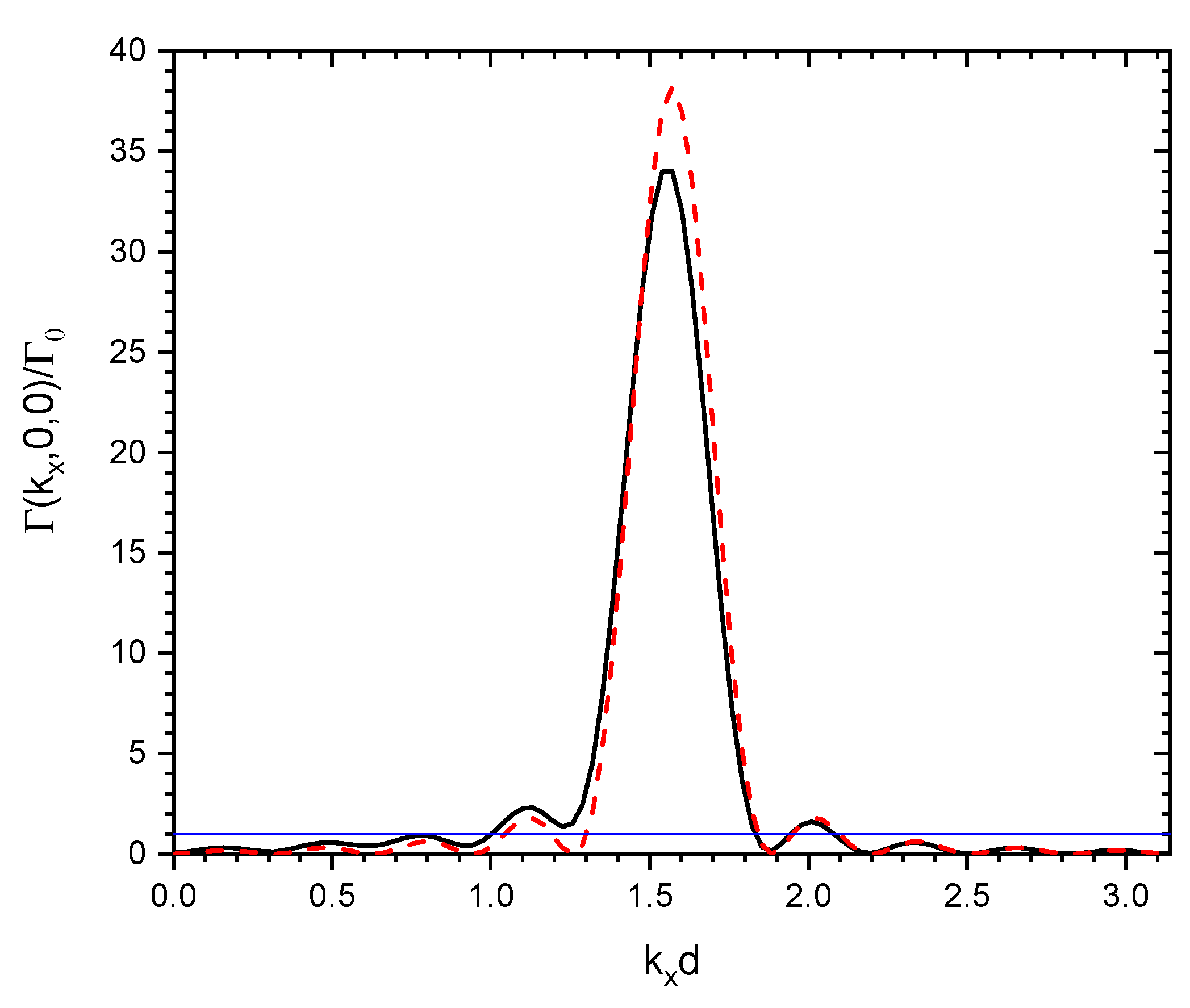
For a large but finite lattice (), and considering modes along the x direction () and with dipoles perpendicular to the 2D array (), an approximate expression for the subradiant region of the spectrum can be derived. Indeed, assuming and in the integral (18) we obtain, for and up to terms (see Appendix A):
where . In the limit (that is, far from the subradiant boundary ), Eq. (24) can be approximated by
which is valid for . Hence, in the subradiant region () the rate scales as . In the superradiant region , for large the expression is close to the solution for an infinite chain (21), which diverges for . Indeed, for and large , Eq. (24) approximates as .
These features are illustrated in Figure 3, where the exact solution of from Eq. (17) [continuous blue line] is compared with the approximate solution (24) [dashed red line] as a function of , in the region . The dash-dotted black line is the infinite chain solution (21), with the vertical dotted line marking the value .
3.5. Finite Square Array: Radial Mode Distribution
For an infinite square array with perpendicularly oriented dipoles [], the rate presents a radial symmetry around – see Eq.(23). Let us exploit this symmetry, now for a finite array, with . Substituting , , and into Eq. (18), we then use the approximation . For a subwavelength step , it leads to
where .
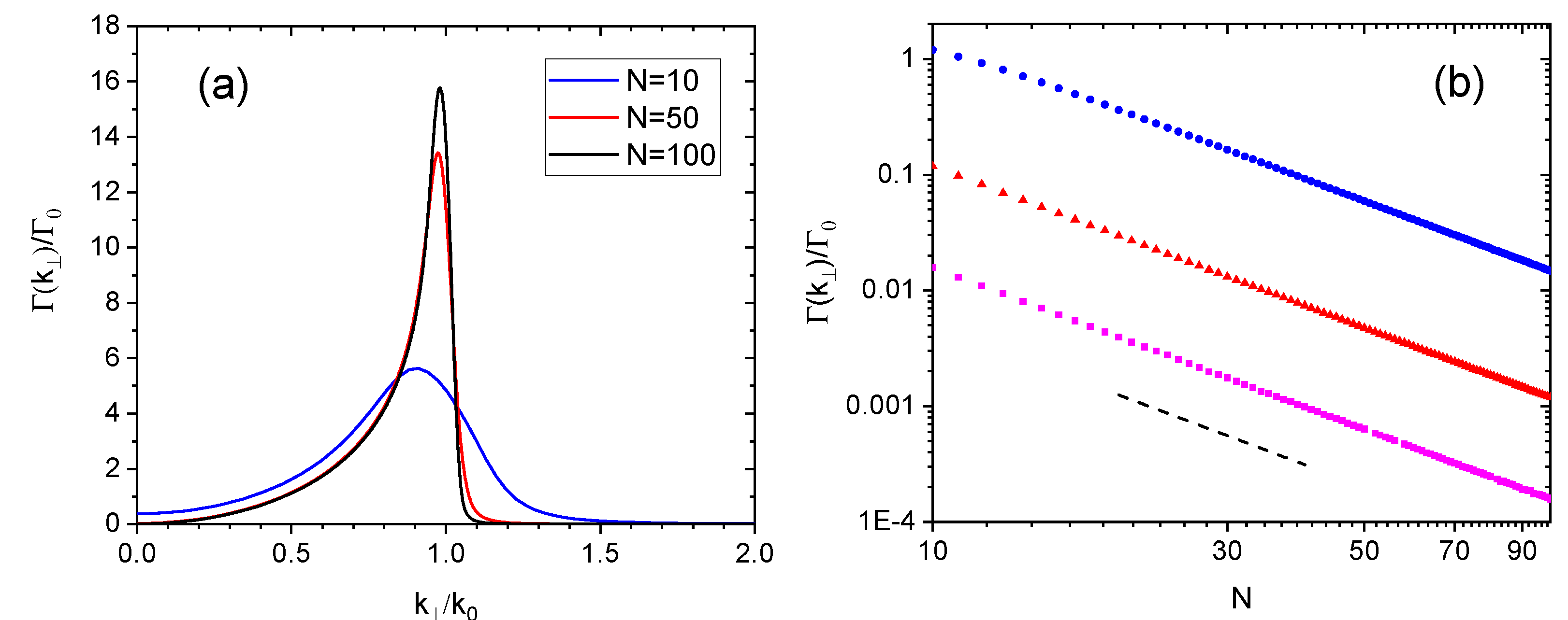
Figure 4(a) shows the behavior of for and different values of N, from a numerical integration of Eq. (26). If we now introduce in Eq. (26), it now takes the form
where is independent on N. This allows us to deduce that in the large N limit, Eq. (27) scales as . This analysis is confirmed by the numerical analysis of Eq. (26), shown in Figure 4(b), where the trend is observed already for .
4. 3D Cubic Atom Array
Let us now consider a 3D cubic array, with atoms at positions with , and . The rate of mode (11) now writes
where
Assuming a large array, , and using the same transformation as in Eq. (18) for 2D arrays, the rate rewrites
where . Here, is the reciprocal lattice vector, with .
4.1. Infinite 3D Array
In the infinite array limit, , one can use the property to simplify rate (30) as
Each term of the sum in Eq. (31) is thus an infinitely-thin shell of center and radius .
We note that in Ref. [15] subradiant modes in infinite 1D and 2D arrays have been described as "guided", since the associated radiation fields are evanescent in the directions transverse to the array. In contrast, in 3D arrays the radiation modes are extended over space, in all directions. Thus, differently from the 1D and 2D cases, the subradiant modes in finite 3D arrays cannot be identified using the results of the infinite arrays, as it has been possible in 1D and 2D arrays. This has lead to focusing on the numerical diagonalization of the scattering matrix to determine the eigenvalues in the finite-N case [15]. In our approach, subradiant modes in a finite 3D array have a finite width around the surface , as we will discuss in the next section.
4.2. Decay Rate for Mode Along an Axis of the Finite Cubic Array
Considering a cubic array with a large size, , an approximate solution for the decay rate can be derived from Eq. (30). In the subradiant region of the spectrum, with and considering for instance modes with polarization along the z axis and along the one (), we derive, up to terms (see Appendix B):
Note that for , using that is the total number of atoms in the cubic array with edges and , the rate rewrites where is the resonant optical thickness. In contrast, decreases as when moves away from , both inside and outside the shell, toward the dark zone. In Figure 5 the rate as a function of shows the very good agreement between the exact expression (28) and the approximate one (32).
In conclusion, for an infinite 3D array subradiance appears almost everywhere, except when . For a finite cubic array, subradiant states are close to those of the infinite array, but with the sharp surfaces of the spectrum turned into smooth ones, with tails in the dark regions whose widths decrease as the inverse of the atom number N.
5. Conclusion
We have thus characterized the decay rates of 2D and 3D atomic arrays, identifying families of Bloch states with strong subradiance properties. In particular, we have shown that using an integral representation to deal with the sum over the many emitters allows one to obtain explicit expressions for the rates, but also to study finite-size effects in different dimensions. With the recent realization of a subradiant 2D atomic array mirror [22], the development of techniques to study systems too large to be studied directly by numerical diagonalization is a crucial task.
While the present work addressed the single-excitation regime, the possibility to use two-level atoms to manipulate multiple-photons states calls for the extension of such methods to the many-body regime [33,34,35]. In particular, combining the long lifetimes of subradiant modes with the photon-photon interactions achieved through dipolar or Rydberg interactions could allow for the creation of tunable atomic platforms for photon manipulation.
Author Contributions
Conceptualization, N.P. and R.B.; methodology, N.P.; formal analysis, N.P.; investigation, N.P. and R.B.; writing—original draft preparation, N.P. and R.B.; writing—review and editing, N.P. and R.B. All authors have read and agreed to the published version of the manuscript.
Funding
R.B. acknowledge the financial support of the São Paulo Research Foundation (FAPESP) (Grants No. 2022/00209-6 and 2023/03300-7), from the Brazilian CNPq (Conselho Nacional de Desenvolvimento Científico e Tecnológico), Grant No. 313632/2023-5.
Institutional Review Board Statement
Not applicable.
Informed Consent Statement
Not applicable.
Conflicts of Interest
The author declare no conflict of interest.
Appendix A. Approximate Solution Γ(k x,0)
We can obtain an approximate solution of of Eq. (18) for a lattice which is finite, yet assuming large. To this end, we change the integration variable from and to and , which leads to:
where and . In Eq. (A1) the dependence on and is in and , respectively; furthermore, the is appreciable only for . We are looking for an approximate solution for the subradiant region of the spectrum under the condition that in the integral of Eq. (A1) . Let us consider the spectrum along the axis (), for dipoles perpendicular to the 2D array (). Taking , we obtain, up to terms :
Inserted in Eq. (A1), we obtain the rate
where . In the subradiant region, when , using the integrals in Eq. (A3) can be solved exactly as
Appendix B. Approximate Solution Γ(k x,0,0)
An approximate solution of from Eq. (30) can be obtained for a finite cubic lattice assuming large. In the subradiance region of the spectrum, we consider the spectrum along the direction axis () and for dipoles oriented along the z-axis (). Taking , Eq. (30) takes the form
By changing the integration variables as and , we obtain up to terms
where . Introducing , we can write
if we neglect the terms proportional to . Then we obtain for the rate
Changing the integration variable into we obtain
If we also neglect the terms and (large size limit), we obtain
References
- Dicke R. H., Coherence in spontaneous radiation processes. Phys. Rev. 1954, 93, 99. [CrossRef]
- Gross, M.; Haroche, S. Superradiance: An Essay on the Theory of Collective Spontaneous Emission. Phys. Rep. 1982, 93, 301. [Google Scholar] [CrossRef]
- Pavolini, D.; Crubellier, A.; Pillet, P.; Cabaret, L.; Liberman, S. Experimental Evidence for Subradiance. Phys. Rev. Lett. 1985, 54, 1917. [Google Scholar] [CrossRef]
- Crubellier, A. Superradiance and subradiance. III. Small samples J. Phys. B 1987, 20, 971. [Google Scholar]
- Facchinetti, G.; Jenkins, S.D.; Ruostekoski, J. Storing light with subradiant correlations in arrays of atoms. Phys.Rev. Lett. 2016, 117, 243601. [Google Scholar] [CrossRef] [PubMed]
- Jen, H.H.; Chang, M.-S.; Chen, Y.-C. Cooperative single photon subradiant states. Phys. Rev. A 2016, 94, 013803. [Google Scholar] [CrossRef]
- Needham, J.A.; Lesanovsky, I.; Olmos, B. Subradiance-protected excitation transport. New J. Phys. 2019, 21, 073061. [Google Scholar] [CrossRef]
- Cech, M.; Lesanovsky, I.; Olmos, B. Dispersionless subradiant photon storage in one-dimensional emitter chains. Phys. Rev. A 2023, 2023 108, L051702. [Google Scholar] [CrossRef]
- Bettles R., J.; Minàř, J.; Adams C., S.; Lesanovsky, I.; Olmos, B. Topological properties of a dense atomic lattice gas. Phys. Rev. A 2017, 96, 041603(R). [Google Scholar] [CrossRef]
- W. Guerin, M. O. Araùjo, and R. Kaiser, Subradiance in a large cloud of cold atoms. Phys. Rev. Lett. 2016, 116, 083601. [CrossRef]
- Porras, D.; Cirac, J.I. Collective generation of quantum states of light by entangled atoms. Phys. Rev. A 2008, 78, 053816. [Google Scholar] [CrossRef]
- Jenkins, S.D.; Ruostekoski, J. Controlled manipulation of light by cooperative response of atoms in an optical lattice. Phys. Rev. A 2012, 86, 031602(R). [Google Scholar] [CrossRef]
- Bettles, R.J.; Gardiner, S.A.; Adams, C.S. Enhanced optical cross section via collective coupling of atomic dipoles in 2D array. Phys. Rev. Lett. 2016, 116, 103602. [Google Scholar] [CrossRef]
- Shahmoon, E.; Wild, D.S.; Lukin, M.D.; Yelin, S.F. Cooperative resonances in light scattering from two-dimensional atomic arrays. Phys. Rev. Lett. 2017, 118, 113601. [Google Scholar] [CrossRef]
- Asenjo-Garcia A.; Moreno-Cardoner M.; Albrecht A:; Kimble H. J.; Chang D. E. Exponential improvement in photon storage fidelities using subradiance and “selective radiance” in atomic arrays. Phys. Rev. X 2017, 7, 031024.
- Jenkins S.D.; Ruostekoski J.;, Papasimakis N:; Savo S.; Zheludev N.I. Many-Body Subradiant Excitations in Metamaterial Arrays: Experiment and Theory. Phys. Rev. Lett. 2017, 119, 05390.
- Bettles, R.J.; Gardiner, S.A.; Adams, C.S. Cooperative eigenmodes and scattering in one-dimensional atomic arrays. Phys. Rev. A 2016, 94, 043844. [Google Scholar] [CrossRef]
- Das, D.; Lemberger, B.; Yavuz, D.D. Subradiance and Superradiance-to-Subradiance Transition in Dilute Atomic Clouds. Phys. Rev. A 2020, 102, 043708. [Google Scholar]
- Ferioli, G.; Glicenstein, A.; Henriet, L.; Ferrier-Barbut, I.; Browaeys, A. Storage and release of subradiant excitations in a dense atomic cloud. Phys. Rev. X 2021, 11, 021031. [Google Scholar] [CrossRef]
- Zoubi, H.; Ritsch, H. Metastability and Directional Emission Characteristics of Excitons in 1D Optical Lattices. Europhys. Lett. 2010, 90, 23001. [Google Scholar]
- Bettles R., J.; Gardiner S., A.; Adams, C.S. Cooperative Ordering in Lattices of Interacting Two-Level Dipoles. Phys. Rev. A 2015, 92, 063822. [Google Scholar] [CrossRef]
- Rui, J.; Wei, D.; Rubio-Abadal, A.; Hollerith, S.; Zeiher, J.; Stamper-Kurn D., M.; Gross, C.; Bloch, I. ; A Subradiant Optical Mirror Formed by a Single Structured Atomic Layer. Nature 2020, 583, 369. [Google Scholar] [CrossRef]
- Katharina Brechtelsbauer, K.; Malz, D. Quantum simulation with fully coherent dipole-dipole interactions mediated by three-dimensional subwavelength atomic arrays. Phys. Rev. A 2021, 104, 013701. [Google Scholar] [CrossRef]
- Van Coevorden, D.V.; Sprik, R.; Tip, A.; Lagendijk, A. Photonic Band Structure of Atomic Lattices. Phys. Rev. Lett. 1996, 77, 2412. [Google Scholar] [CrossRef]
- Antezza, M.; Castin, Y. Fano-Hopfield model and photonic band gaps for an arbitrary atomic lattice. Phys. Rev. A 2009, 80, 013816. [Google Scholar] [CrossRef]
- Perczel, J.; Borregaard, J.; Chang, D.E.; Pichler, H.; Yelin, S.F.; Zoller, P.; Lukin, M.D. Photonic band structure of two-dimensional atomic lattices. Phys. Rev. A 2017, 96, 063801. [Google Scholar] [CrossRef]
- Piovella, N. Cooperative Decay of an Ensemble of Atoms in a One-Dimensional Chain with a Single Excitation. Atoms 2024, 12, 43. [Google Scholar] [CrossRef]
- Zhang Y.X., Mölmer K. Phys. Rev. Lett. 2020, 125, 253601.
- Akkermans, E.; Gero, A.; Kaiser, R. Photon localization and Dicke superradiance in atomic gases. Phys. Rev. Lett. 2008, 101, 103602. [Google Scholar] [CrossRef] [PubMed]
- Rouabah, M.T.; Samoylova, M.; Bachelard, R.; Courteille, P.W.; Kasier, R.; Piovella, N. Coherence effects in scattering order expansion of light by atomic clouds, J. Opt. Soc. Am. A 2014, 31, 1031. [Google Scholar] [CrossRef]
- Scully, M.O.; Fry, E.; Ooi, C.H.R.; Wodkiewicz, K. Directed Spontaneous Emission from an Extended Ensemble of N Atoms: Timing Is Everything. Phys. Rev. Lett. 2006, 96, 010501. [Google Scholar] [CrossRef] [PubMed]
- Scully, M.O. Single photon subradiance: quantum control of spontaneous emission and ultrafast readout. Phys. Rev. Lett. 2015, 115, 243602. [Google Scholar] [CrossRef]
- Walther, V.; Zhang, L.; Yelin, S.F.; Pohl, T. Nonclassical light from finite-range interactions in a two-dimensional quantum mirror. Phys. Rev. B 2022, 105, 075307. [Google Scholar] [CrossRef]
- Zhang, L.; Walther, V.; Mölmer, K.; Pohl, T. Photon-photon interactions in Rydberg-atom arrays. Quantum 2022, 6, 674. [Google Scholar] [CrossRef]
- Pedersen, S.P.; Zhang, L.; Pohl, T. Quantum nonlinear metasurfaces from dual arrays of ultracold atoms. Phys. Rev. Res. 2022, 5, L012047. [Google Scholar] [CrossRef]
Figure 1.
Collective decay rate in the plane for the infinite array with (a) and (b) , and dipoles oriented along the x-axis.
Figure 1.
Collective decay rate in the plane for the infinite array with (a) and (b) , and dipoles oriented along the x-axis.
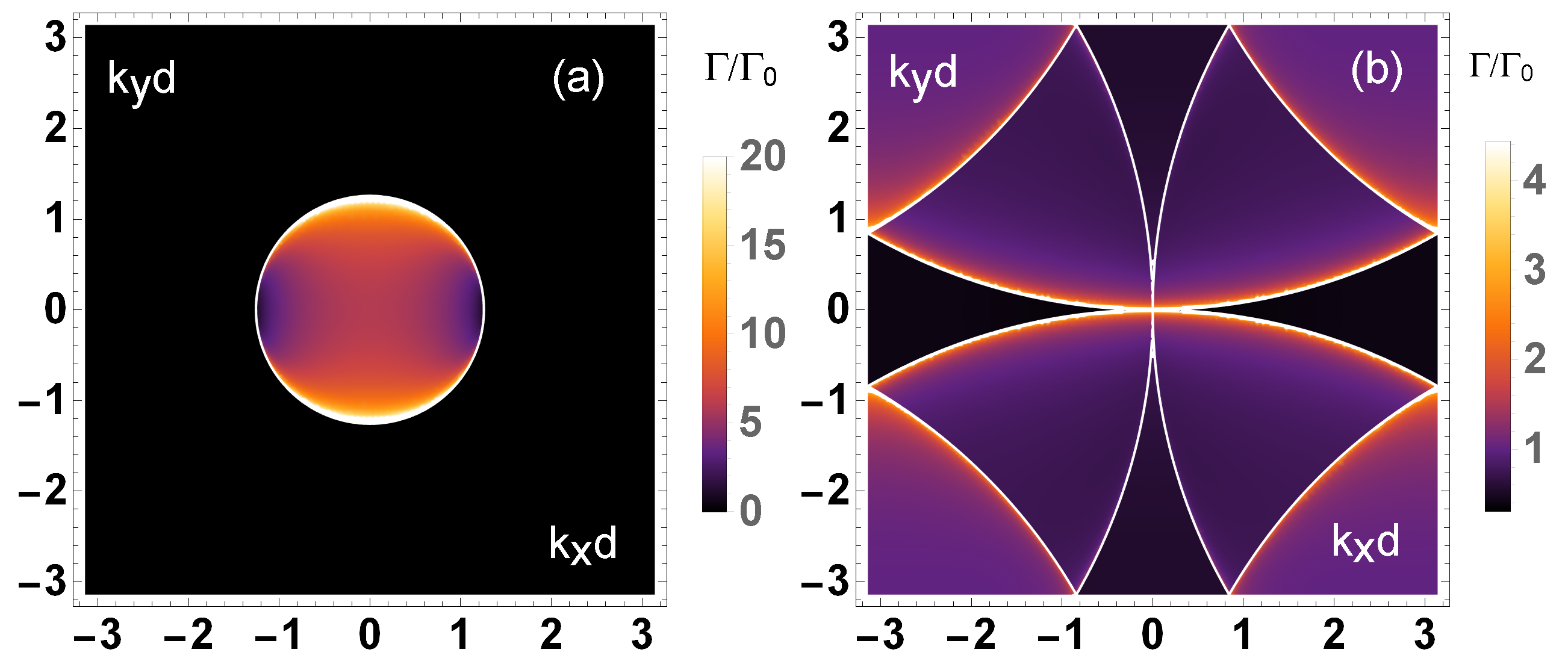
Figure 2.
vs for a square lattice with and polarization (a) perpendicular to the plane, , and (b) within the atomic plane, . The dashed red lines are the solution for an infinite lattice, provided by Eq. 21). In the case (a), when for an infinite lattice.
Figure 2.
vs for a square lattice with and polarization (a) perpendicular to the plane, , and (b) within the atomic plane, . The dashed red lines are the solution for an infinite lattice, provided by Eq. 21). In the case (a), when for an infinite lattice.
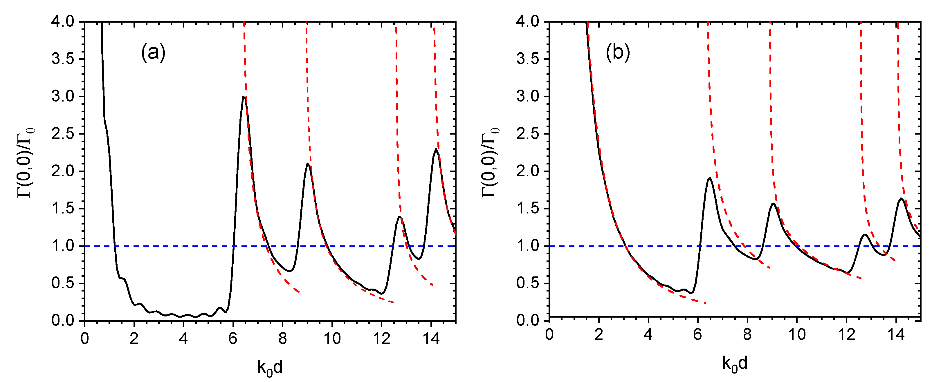
Figure 3.
Collective decay rate as a function of , for a square array with and , with a polarization orthogonal to the array (). Full blue line: exact solution (18); Red dashed line: approximate solution (24); Dash-dotted line: solution for the infinite chain (21). The vertical dotted line stands for the value .
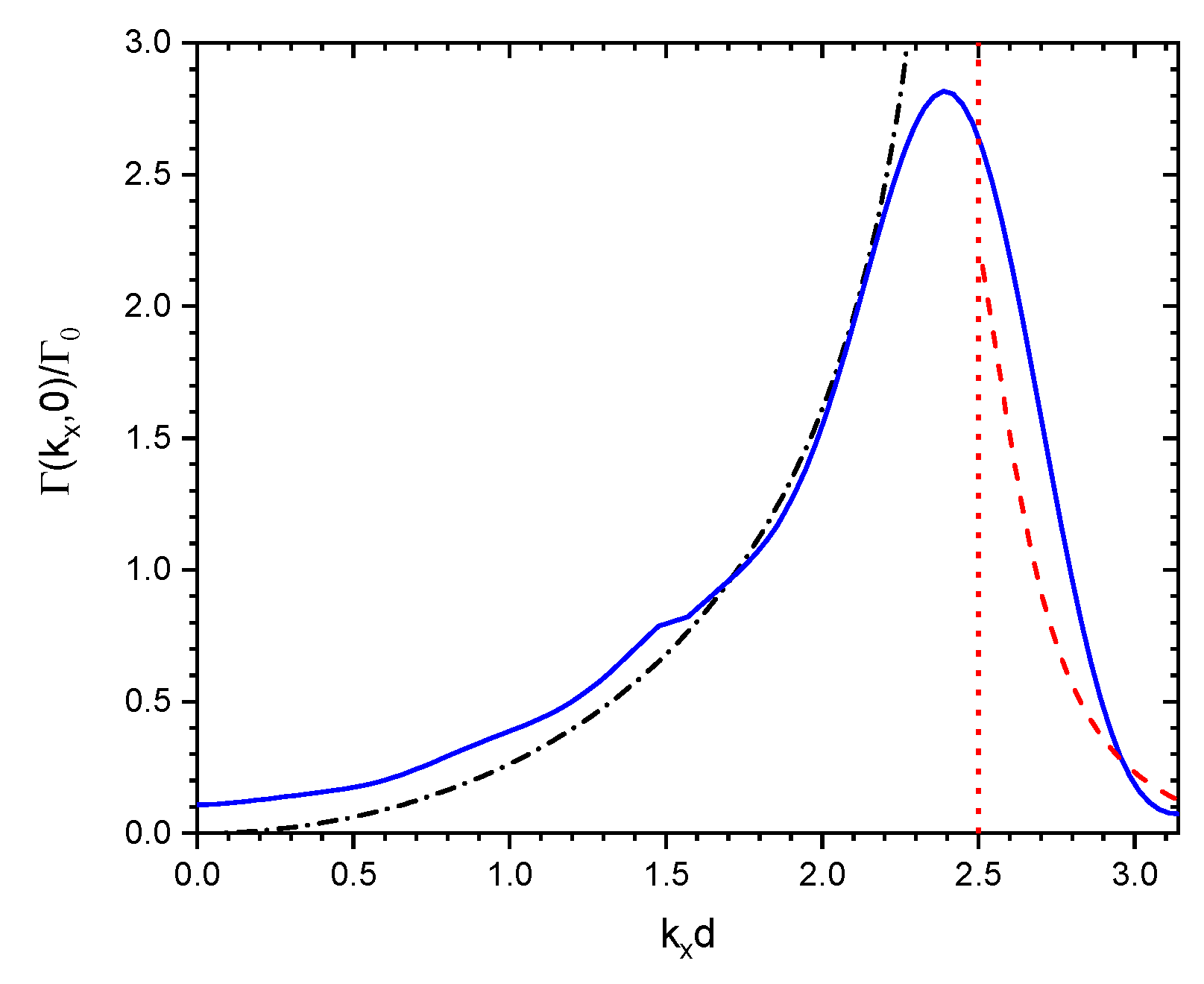
Figure 4.
Collective decay rate as a function (a) of for a square array and (blue line), (red line) and (black line), and (b) of N for (pink boxes), (red triangles) and 2 (black circles); the dashed line in (b) shows the dependence. All simulations realized for .
Figure 4.
Collective decay rate as a function (a) of for a square array and (blue line), (red line) and (black line), and (b) of N for (pink boxes), (red triangles) and 2 (black circles); the dashed line in (b) shows the dependence. All simulations realized for .
Disclaimer/Publisher’s Note: The statements, opinions and data contained in all publications are solely those of the individual author(s) and contributor(s) and not of MDPI and/or the editor(s). MDPI and/or the editor(s) disclaim responsibility for any injury to people or property resulting from any ideas, methods, instructions or products referred to in the content. |
© 2025 by the authors. Licensee MDPI, Basel, Switzerland. This article is an open access article distributed under the terms and conditions of the Creative Commons Attribution (CC BY) license (https://creativecommons.org/licenses/by/4.0/).
Copyright: This open access article is published under a Creative Commons CC BY 4.0 license, which permit the free download, distribution, and reuse, provided that the author and preprint are cited in any reuse.


