A Novel Decomposition-Integration Based Transformer Model for Multi-Scale Electricity Demand Prediction

1. Introduction

With China’s rapid economic development driving accelerated growth in electricity demand, electricity sales forecasting [1] has evolved into a critical component for power system planning and operational management. As a core performance metric for grid operators, sales volume data underpins performance evaluation, profit equi-librium regulation, and electricity marketing strategies, while simultaneously guiding daily operational and production activities—including resource allocation and emer-gency response protocols. Accurate forecasting enables optimized grid infrastructure planning, evidence-based enterprise operations management, rational power trans-mission/distribution network allocation, and accelerated electricity market reform [2].

However, actual sales volume data manifests significant multidimensional heteroge-neity due to the compound effects of meteorological conditions, external economic fluctuations, grid operational indicators, and holiday impacts. This complexity arises from interconnected mechanisms wherein temperature variations and holi-day-induced regime shifts reshape societal consumption patterns, while economic tra-jectories and grid operational status collectively drive usage scale volatility. Dynami-cally, these interacting forces generate highly coupled trend components, periodic os-cillations, and stochastic perturbations within the time series. Conventional forecasting approaches—including Long Short-Term Memory (LSTM) [3] models, Autoregressive Integrated Moving Average (ARIMA) models, and Transformer-based mod-els—frequently encounter challenges when processing strongly coupled data, such as overfitting, sensitivity to noise, and excessive computational complexity. Furthermore, long-term sequential data often faces memory bottlenecks and is highly susceptible to external interference, leading to data distribution drift. These limitations hinder simple models from capturing long-term temporal dependencies, resulting in persistent chal-lenges in achieving both accurate and efficient predictions.

To address these challenges, this paper proposes a decomposition-integration-based transformer framework. Initially, the methodology employs Variational Mode De-composition (VMD) [4] coupled with the Zebra Optimization Algorithm (ZOA) to adaptively decompose the original electricity sales sequence. This process mitigates data non-stationarity and extracts representative subsequences with clearer structural characteristics, thereby establishing a robust foundation for subsequent modeling. Subsequently, an improved RevInformer model is utilized to separately model and forecast each derived subsequence. The predictions from all components are then in-tegrated to generate the final output. The primary contributions of this study are summarized as follows:

1)

A novel electricity sales forecasting method is proposed, employing a decomposi-tion-integration framework. This approach adaptively decomposes the original se-quence by integrating Variational Mode Decomposition (VMD) with the Zebra Opti-mization Algorithm (ZOA), thus significantly reducing modeling complexity. Subse-quently, an improved RevInformer model performs component-wise prediction on each subsequence, with final forecasts generated through aggregated integration of all component predictions.

2)

An enhanced RevInformer model is developed by introducing Reversible Layers to the Informer architecture, strengthening deep feature propagation capabilities. Simulta-neously, a bidirectional modeling mechanism is incorporated, effectively improving modeling capacity and prediction accuracy for complex non-stationary sequences.

3)

The proposed methodology was validated using an annual electricity sales dataset from a commercial building. Experimental results demonstrate that our approach achieves 60%–90% improvements across all evaluation metrics, surpassing the per-formance of existing benchmark methods.

The remainder of this paper is structured as follows. Section 2 reviews existing tech-niques in demand forecasting. Section 3 presents the system model and primary re-search methodology. Section 4 verifies the feasibility and effectiveness of the pro-posed approach through experimental validation. Section 5 concludes the study and outlines future research directions.

2. Related Work

Accurate forecasting in power systems is critical for grid stability and economic dispatch. However, the unique characteristics of power data—including high volatility, complex multi-scale seasonality, and susceptibility to external factors like weather and economic activity—pose significant challenges to conventional forecasting models.

Early studies primarily relied on traditional statistical methods. The ARIMA model [5], for instance, became a benchmark for time series forecasting and was ap-plied to tasks such as carbon emission prediction [6]. While enhanced by techniques like wavelet decomposition for handling transients [7], these models are fundamentally limited to univariate, stationary series, failing to capture the complex nonlinearities in power data. The advent of machine learning, marked by decision trees [8] and en-semble methods like random forests [9,10], improved predictive performance by model-ing more complex relationships. Concurrently, Recurrent Neural Networks (RNNs), with the Elman network [11] as a prototype, introduced a mechanism for processing sequential data. However, vanilla RNNs suffer from gradient vanishing [12], limiting their capacity to learn long-term dependencies in historical load data.

To overcome these limitations, more sophisticated neural architectures were in-troduced. Long Short-Term Memory (LSTM) networks [13], enhanced by the forget gate [14], provided a robust solution for capturing long-range dependencies and mit-igating temporal noise. Parallelly, Convolutional Neural Networks (CNNs) [15] were adapted to extract local temporal patterns. Despite their strengths, these models often remain inadequate for modeling the intricate, long-range dependencies present in large-scale, multi-variable power system data.

The Transformer architecture [16] emerged as a breakthrough, replacing recur-rence with self-attention to efficiently capture global dependencies. Its superiority has led to numerous adaptations in load forecasting. For example, some works integrate seasonal decomposition with Transformer to model periodic characteristics [17], while others employ federated learning frameworks to alleviate data scarcity in new regions [18]. Despite these advances, the standard Transformer and its early variants, such as Informer [19], face persistent challenges. Informer’s generative decoder and sparse at-tention improve long-sequence forecasting efficiency, but its massive memory con-sumption and slow execution become prohibitive with the high-dimensional data typical in power systems [20]. Furthermore, while hybrid models that combine decomposition techniques (e.g., CEEMDAN) with Informer can enhance noise ro-bustness [21], they often treat decomposition and modeling as separate, sub-optimal stages, and still struggle with complex, non-stationary dynamics.

This has spurred the development of decomposition-integration frameworks, which leverage signal processing techniques to decompose complex sequences into simpler sub-sequences for individual modeling, significantly enhancing predictive performance. This approach has demonstrated effectiveness across multiple domains. For instance, it has been integrated with Prophet and Stacking for electricity price forecasting [22], combined with VMD-BiLSTM-TCN for stock market prediction [23], and utilized with EEMD for financial trend analysis [24] and mass spectrometer data enhancement [25].

However, a pivotal challenge in these frameworks often remains unaddressed: distribution shift. The statistical properties of the decomposed sub-series can differ significantly from each other and from the original data, a problem particularly acute in volatile power load sequences. This can compromise the reliability of forecasts from standard models trained on these components.

To address the dual challenges of long-sequence forecasting efficiency and dis-tribution shift in decomposed components, this paper introduces the RevInformer model for power load forecasting. Our framework incorporates Variational Mode Decomposition (VMD) in the data preprocessing phase. The decomposed components are then processed by the RevInformer architecture [26], which implements Reversible Instance Normalization (RevIN). This mechanism allows the model to dynamically adapt to non-stationary sub-series, effectively resolving distribution shifts and signifi-cantly enhancing the reliability of predictions for complex power system data.

3. Methodology

3.1. The Framework for the Proposed Method

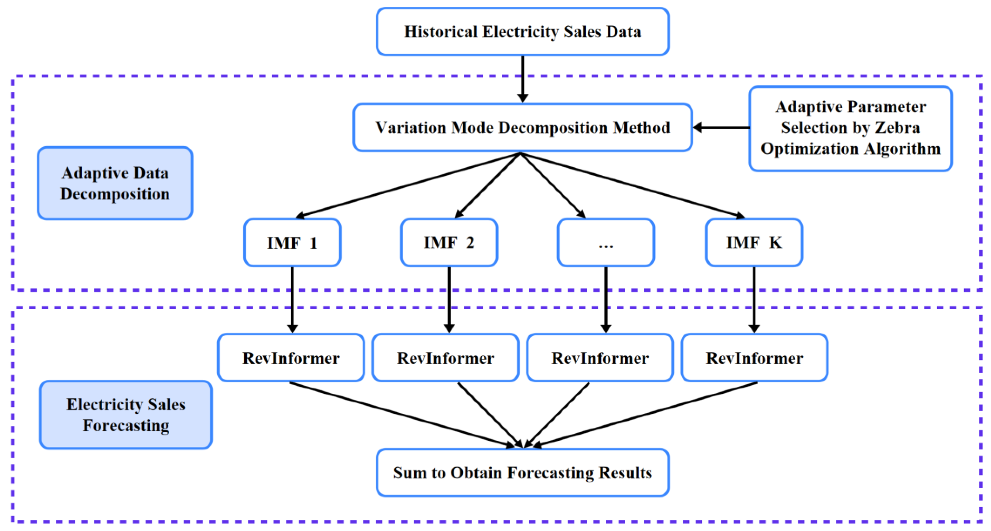
Affected by natural conditions, human activities, unexpected events, and other factors, electricity sales data exhibits pronounced non-stationarity and nonlinearity, rendering sales forecasting highly challenging. Given the difficulty in capturing volatility patterns from raw data, this study adopts a decomposition-integration framework. First, the model employs VMD to adaptively decompose long time-series data, utilizing ZOA for optimized parameter selection to achieve peak performance. Subsequently, the raw data—decomposed into designated IMFs—is independently fed into the RevInformer model for separate training and prediction. Finally, predicted subsequences are aggregated through summation to yield the final forecast. This framework effectively mitigates sequence non-stationarity, adapts to data distribution variations, and enhances predictive performance. The detailed workflow is illustrated in Figure 1.

3.2. Adaptive Data Decomposition

The core objective of adaptive data decomposition is to dynamically adjust decomposition strategies for more accurate identification of hidden patterns in complex data, thereby enhancing subsequent forecasting precision. Traditional decomposition methods struggle to handle cyclical variations or abrupt trends, whereas adaptive decomposition provides flexible adaptation to data dynamics while avoiding overfitting in complex data scenarios, thus strengthening model generalization capabilities.

Parameter selection proves critical to decomposition effectiveness during this process. For VMD-based methods:

4)

Insufficient subsequence settings increase reconstruction errors.

5)

Excessive settings substantially escalate computational overhead.

Manual parameter determination fails to optimally balance reconstruction error and computational complexity. Therefore, this study integrates ZOA with VMD decomposition to automatically select optimal configurations based on raw data characteristics. This approach effectively manages computational costs while guaranteeing reconstruction precision.

3.2.1. Variational Mode Decomposition

Variational Mode Decomposition (VMD) employs a variational optimization framework to decompose signals into distinct modes with specific center frequencies while minimizing the total bandwidth of all modes. It is commonly used to decompose complex non-stationary signals into multiple Intrinsic Mode Functions (IMFs) characterized by sparsity and band-limited properties. Compared to traditional Empirical Mode Decomposition (EMD), VMD demonstrates stronger robustness against noise and non-stationary signals. The IMF obtained via VMD decomposition is expressed as:

$$u_k\left(t\right)=A_k\left(t\right)\cos \left({\varnothing }_k\left(t\right)\right)$$

(1)

where $A_k\left(t\right)$ represents the instantaneous amplitude of $u_k\left(t\right)$, and ${\varnothing }_k\left(t\right)$ is a non-decreasing phase function. To enhance decomposition precision, VMD incorporates a penalty factor (α) and Lagrangian multiplier (λ) to formulate a highly nonlinear constrained variational problem. The algorithm minimizes the following function:

$$L\left(\left\{u_k\right\},\left\{{\omega }_k\right\},\lambda \right)=\alpha {\sum }_k{‖\left[{\partial }_t(\sigma \left(t\right)+{\displaystyle \frac{j}{\pi t}})\bullet u_k\left(t\right)\right]e^{-j{\omega }_{t}t}‖}_2^2+{‖f\left(t\right)-{\sum }_k{u}_k\left(t\right)‖}_2^2+〈\lambda \left(t\right),f\left(t\right)-{\sum }_k{u}_k\left(t\right)〉$$

(2)

where α denotes the penalty factor, and λ(t) is the Lagrangian multiplier.

The Alternating Direction Method of Multipliers (ADMM) iteratively updates the mode functions $u_k$, center frequencies ${\omega }_k$, and Lagrangian multiplier $\lambda$ to solve the constrained variational problem. The iterative formulas are:

$$\left\{\begin{array}{c}{\widehat{\mathrm{u}}}_{\mathrm{k}}^{\mathrm{n}+1}={\displaystyle \frac{\widehat{\mathrm{f}}\left(\mathrm{x}\right)-{\sum }_{\mathrm{i}<\mathrm{k}}{\widehat{\mathrm{u}}}_{\mathrm{k}}^{\mathrm{n}+1}\left(\mathsf{\omega }\right)+\frac{{\widehat{\mathsf{\lambda }}}^{\mathrm{n}}\left(\mathsf{\omega }\right)}{2}}{1+2\mathsf{\alpha }{\left(\mathsf{\omega }-{\mathsf{\omega }}_{\mathrm{k}}^{\mathrm{n}}\right)}^2}}\\ {\mathsf{\omega }}_{\mathrm{k}}^{\mathrm{n}+1}={\displaystyle \frac{{\int }_0^{\mathrm{\infty }}\mathsf{\omega }{\left|{\widehat{\mathrm{u}}}_{\mathrm{k}}^{\mathrm{n}+1}\left(\mathsf{\omega }\right)\right|}^2\mathrm{d}\mathsf{\omega }}{{\int }_0^{\mathrm{\infty }}{\left|{\widehat{\mathrm{u}}}_{\mathrm{k}}^{\mathrm{n}+1}\left(\mathsf{\omega }\right)\right|}^2\mathrm{d}\mathsf{\omega }}}\\ {\widehat{\mathsf{\lambda }}}^{\mathrm{n}+1}={\widehat{\mathsf{\lambda }}}^{\mathrm{n}}\left(\mathsf{\omega }\right)+\tau (\widehat{\mathrm{f}}\left(\mathsf{\omega }\right)-\sum _{\mathrm{k}}{\widehat{\mathrm{u}}}_{\mathrm{k}}^{\mathrm{n}+1}\left(\mathsf{\omega }\right)\end{array}\right.$$

(3)

where $\widehat{\mathrm{u}}$, $\widehat{\mathrm{f}}$ and ${\widehat{\mathsf{\lambda }}}^{\mathrm{n}}$ are the Fourier transforms of $u_k\left(t\right)$, $f\left(t\right)$, and $\lambda \left(t\right)$ respectively; $\tau$ denotes the noise-tolerance parameter; and$n$ indicates the iteration index.

Iterations continue until the stopping criterion is satisfied:

$${\displaystyle \frac{{\sum }_{k-1}^L{‖{\widehat{\mathrm{u}}}_{\mathrm{k}}^{\mathrm{n}+1}-{\widehat{\mathrm{u}}}_{\mathrm{k}}^{\mathrm{n}}‖}_2^2}{{‖{\widehat{\mathrm{u}}}_{\mathrm{k}}^{\mathrm{n}}‖}_2^2}}<\epsilon$$

(4)

where ε is a predefined tolerance constant for convergence. The process terminates upon meeting this condition, yielding K final IMFs.

3.2.2. Self-Adaptive Parameter Selection Using Zebra Optimization Algorithm

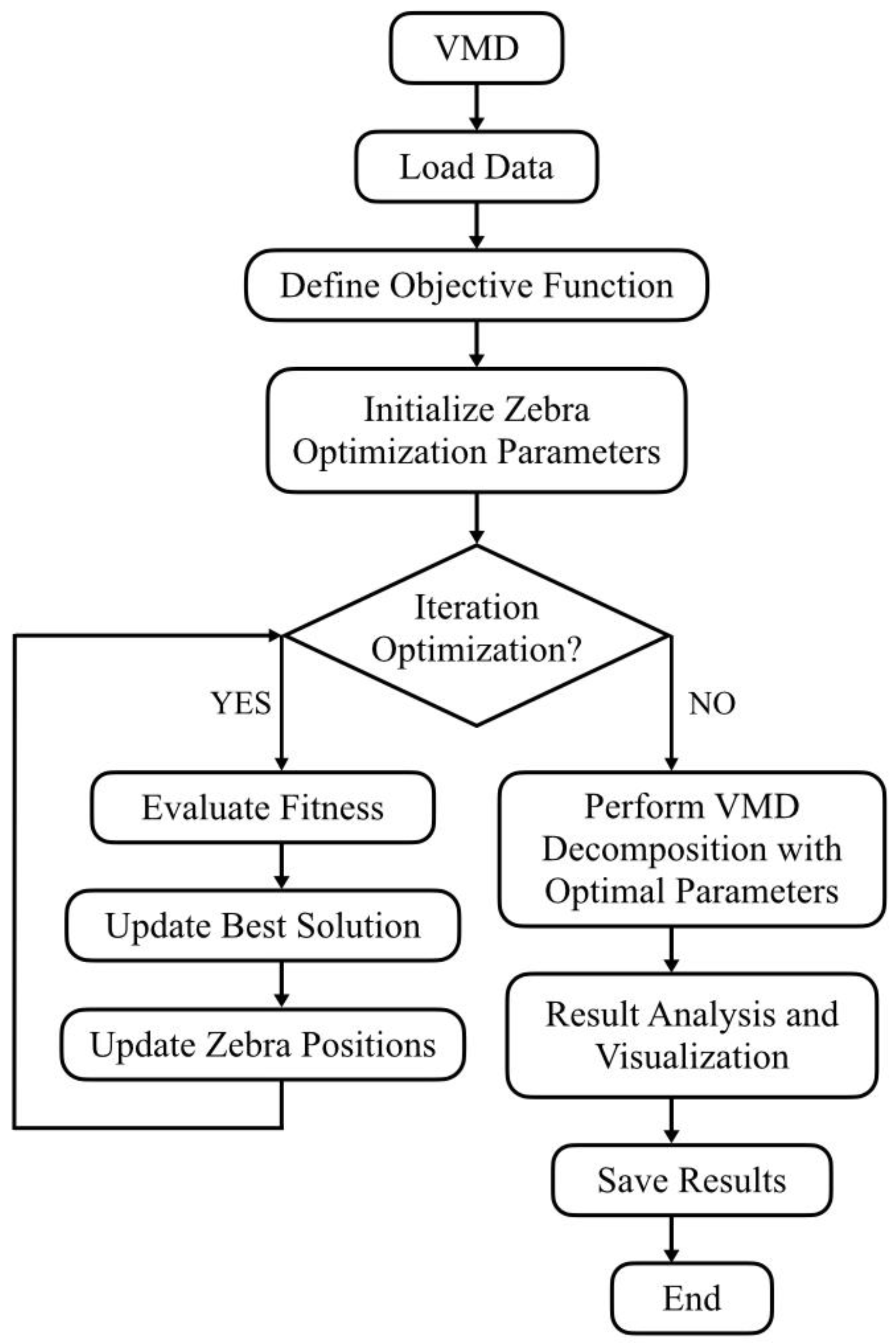
When applying VMD to electricity sales data, the selection of critical parameters—mode number K and penalty factor α—is essential. This study introduces the Zebra Optimization Algorithm (ZOA) to optimize these parameters by simulating zebra herd behaviors through three stages: parameter initialization, iterative optimization, and result recording/output.

Optimization Workflow:

1)

Initialization: Randomly generate 15 parameter combinations ($K$,$\alpha$) within predefined bounds.

2)

Iteration: Dynamically adjust combinations toward optimal solutions.

3)

Evaluation: For each combination, compute RMSE to assess performance.

4)

Finalization: Deploy the optimal combination ($K^{*}$, ${\alpha }^{*}$) for VMD signal decomposition.

Post-Decomposition Validation: calculate performance metrics including Root Mean Square Error (RMSE), Signal-to-Noise Ratio (SNR), Mean Absolute Error (MAE), Maximum Absolute Error (MaxAE).

The complete procedure is illustrated in Figure 2.

Compared to traditional optimization algorithms, the ZOA demonstrates distinct advantages in the following aspects:

1）When searching for the optimal solution, ZOA extends its scope to the global range. The exploration phase of ZOA, characterized by long-distance jump properties, enables the algorithm to escape current local optimum regions and expand the search boundary. In contrast, traditional Particle Swarm Optimization (PSO) relies on particle historical and social experiences, making it prone to stagnation in current regions and often limiting exploration outcomes to local optima.

2）As a meta-optimizer, ZOA possesses fewer parameters and a clearer structure, eliminating the need for additional computational overhead to tune its own parameters. However, the Genetic Algorithm (GA) involves parameters such as crossover rate and mutation rate during the optimization process. Tuning these parameters can compromise the algorithm’s robustness and lead to an “infinite recursion” dilemma.

The typical steps of ZOA—initialization, iterative update, and evaluation selection—endow it with a broader perspective, more reliable convergence, and overall robustness when addressing complex, black-box parameter optimization problems.

3.3. Electricity Sales Forecasting

Following adaptive decomposition of electricity sales data, k independent IMFs are obtained. Each component is individually trained and predicted. This study introduces standardization and destandardization operations for model inputs/outputs based on the Informer architecture, termed the RevInformer model. This model generates k independent predictions, which are then summed to yield final forecasting results.

3.3.1. RevInformer

Forecasting tasks often involve long time series characterized by extensive data coverage and high complexity. Transformer models leveraging self-attention mechanisms capture global dependencies to avoid gradient vanishing. However, self-attention exhibits $O\left(n^2\right)$ complexity, leading to high memory consumption and low efficiency for long sequences, while iterative decoding causes significant error accumulation. To address these issues, the improved Informer model replaces standard self-attention with ProbSparse self-attention, reducing complexity to $O\left(n\log n\right)$. The sparsity metric $M(qi,K)$ evaluates query vector importance:

$$M\left(qi,K\right)=\ln {\sum }_{j=1}^{K_K}{e}^{{\displaystyle \frac{Q_i{K}_j^T}{\sqrt{d}}}}-{\displaystyle \frac{1}{L_K}}{\sum }_{j=1}^{L_K}{\displaystyle \frac{Q_i{K}_j^T}{\sqrt{d}}}$$

(5)

where $qi$ denotes the i-th query, $K$ the key matrix, and $L_K$ the key length. This yields the ProbSparse self-attention formula:

$$Attention\left(Q,K,V\right)=Softmax\left({\displaystyle \frac{Q{K}^T}{\sqrt{d}}}\right)V$$

(6)

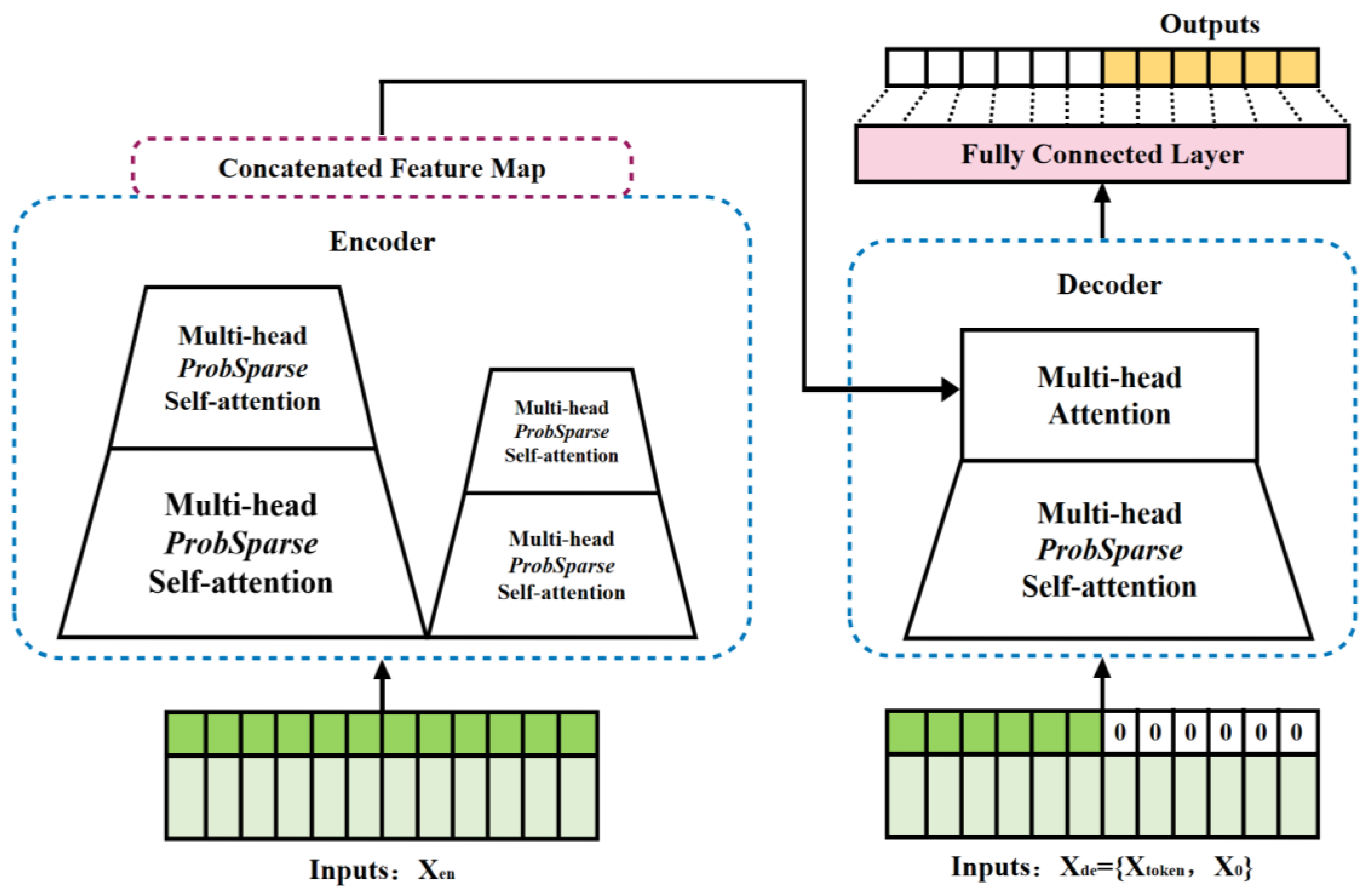
As depicted in Figure 3, Informer’s self-attention distillation compresses feature dimensions layer-wise, halving input sequence length per encoder to reduce memory usage while preserving essential information. Its generative decoder outputs full prediction sequences in a single step, eliminating iterative decoding errors and accelerating inference. The encoder (left) processes long inputs via sparse attention, while the decoder (right) generates predictions autoregressively.

However, existing forecasting models remain vulnerable to distribution shift—temporal variations in statistical properties across long sequences. This discrepancy between training and inference phases causes model instability. Additionally, input sequence heterogeneity degrades performance. While removing non-stationary signals reduces variability, critical predictive information may be lost.

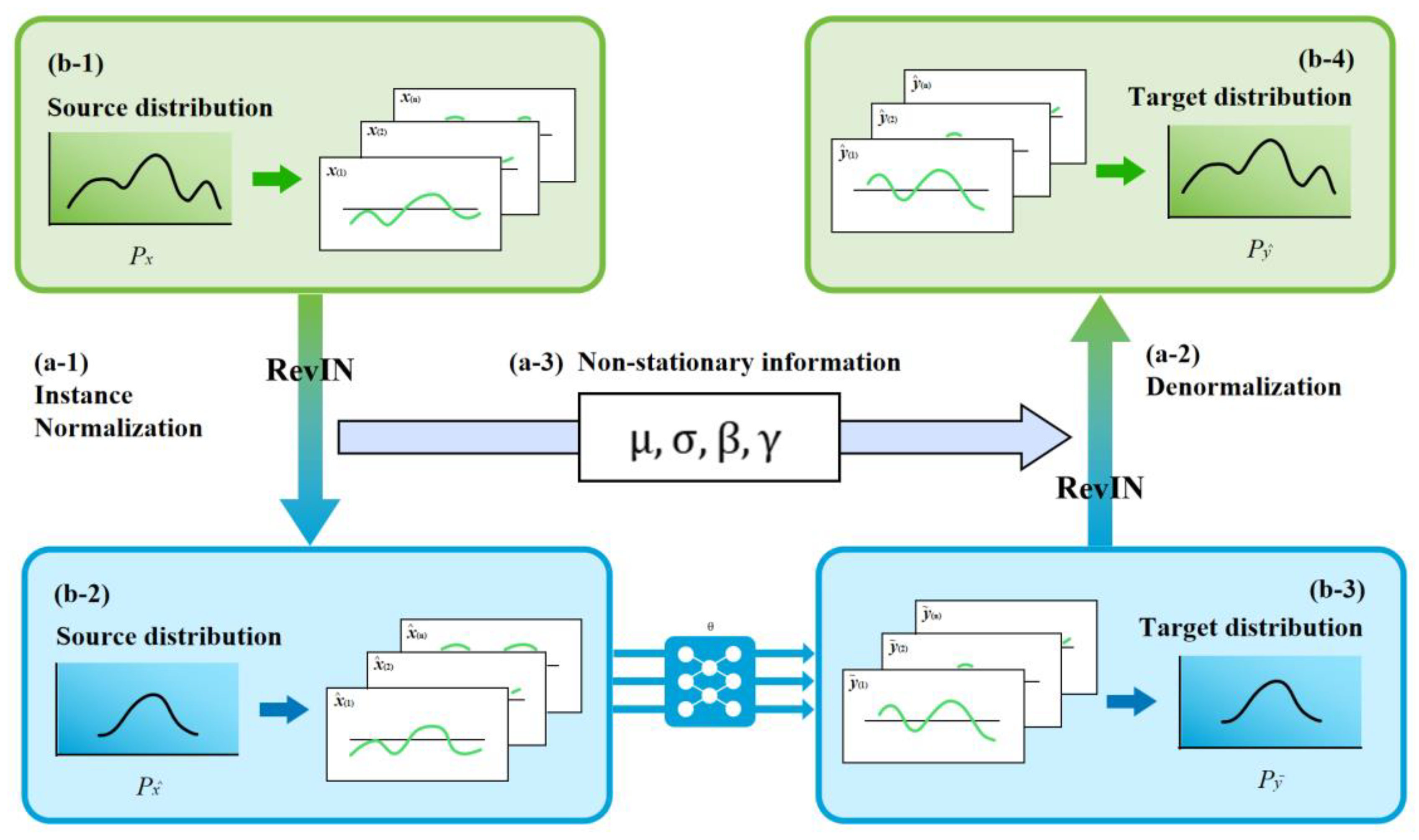
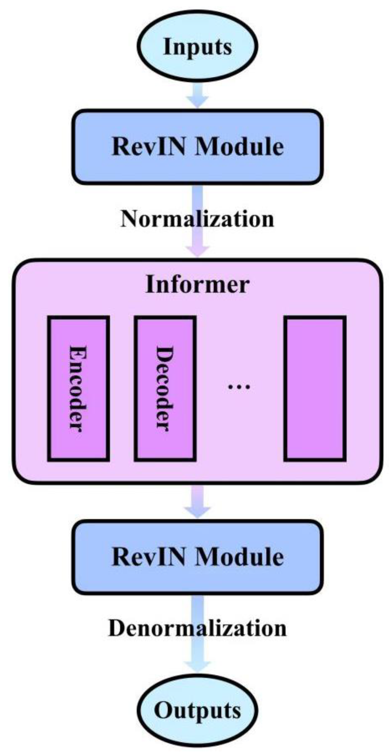
To resolve this, RevInformer incorporates Reversible Instance Normalization (RevIN) (Figure 4). The source distribution (b-1, b-2) represents raw inputs exhibiting non-stationary mean and variance. The target distribution (b-3, b-4) requires alignment with the source to mitigate distribution shift.

Process (a-1): Instance Normalization. For each input instance, this operation is defined as:

$$x^{\text{'}}={\displaystyle \frac{x-\mu }{\sigma }}$$

(7)

where $\mu \left(i\right)$ and $\sigma \left(i\right)$ represent the input sequence’s mean and standard deviation, respectively.

Process (a-2): Denormalization. This operation acts upon model outputs as follows:

$$y=y^{\text{'}}\bullet \sigma +\mu$$

(8)

restoring data to its original scale to preserve distribution information.

Process (a-3): Parameter Storage and Adaptation. Stores parameters $\mu \left(i\right)$ and $\sigma \left(i\right)$ extracted during standardization, while incorporating learnable scaling $\left(\gamma \right)$ and shift $\left(\beta \right)$ parameters to enhance adaptability to distribution shifts.​

The RevIN module executes standardization upon receiving input sequences. After internal model processing, destandardization is applied to outputs. This symmetric workflow ensures:

Elimination of input-output distribution discrepancies;

Effective resolution of ​​distribution shift​​ in forecasting;

Preservation and reversible recovery of non-stationary information;

Mitigation of information loss through parameter retention.

Particularly suited for long-horizon forecasting tasks (e.g., electricity sales prediction) impacted by non-stationarity, this mechanism guarantees that decomposed IMF components can be accurately reconstructed via destandardization after independent prediction.

3.3.2. RevInformer-Based Sales Forecasting

Electricity sales forecasting necessitates extensive historical data derived from daily consumer records, characterized by abrupt fluctuations, strong coupling, and heightened sensitivity to external disturbances that compromise predictive accuracy. Following VMD-based decomposition into K mutually independent IMFs—ensuring spectral separation without informational overlap—this study employs the RevInformer model for individual IMF prediction.

During data loading and preprocessing, the univariate forecasting mode is configured by invoking relevant functions to load datasets and define critical parameters: input sequence length, prediction horizon, training epochs, and dataset partitions. Each IMF undergoes independent model retraining and validation prior to prediction to ensure component isolation. Concurrently, the RevIN module executes instance-specific normalization on each subsequence, persistently storing instance-wise mean (μ) and standard deviation (σ) parameters throughout the process.

Formal prediction proceeds through batched data processing via the encoder-decoder architecture:

The encoder leverages ProbSparse self-attention to extract global dependencies from historical sequences.

The decoder adopts a semi-autoregressive mechanism: initial tokens guide sequential prediction, with intermediate outputs iteratively interacting with encoder states to generate predictions.

Post-prediction, the symmetrical RevIN component denormalizes outputs using stored μ and σ values restoring original scales. Results are exported as NumPy arrays, effectively mitigating distribution shift inherent in conventional models.

The integrated RevInformer framework architecture is illustrated in Figure 5.

The final predictions are obtained by summing the k denormalized prediction sequences output by RevInformer:

$${\widehat{y}}_{total}={\sum }_{i=1}^k{\widehat{y}}^{\left(i\right)}$$

(9)

where ${\widehat{y}}^{\left(i\right)}$ denotes the i-th denormalized prediction sequence. Linear superposition of these sequences yields the ultimate target prediction series.

4. Experimental Verification

4.1. Dataset Introduction

The data employed in this study characterizes provincial electricity consumption patterns over a recent three-year period, encompassing daily usage volumes, peak load points, service disruptions due to payment defaults or technical failures, and sector-specific consumption across industries. This comprehensive dataset comprises approximately 1,100 daily interval measurements. Throughout experimentation, all data points were partitioned into training, testing, and validation sets at a ratio of 7:2:1 for model development and evaluation purposes.

4.2. Experimental Setup

4.2.1. Performance Indicators

To rigorously evaluate the predictive performance of the RevInformer model, five key accuracy metrics are adopted: Mean Absolute Error (MAE), Mean Squared Error (MSE), Root Mean Squared Error (RMSE), Mean Absolute Percentage Error (MAPE), Mean Squared Percentage Error (MSPE). These metrics provide statistically robust evaluation criteria, with their formal definitions and computational formulas detailed below to elucidate their utility in error quantification and model reliability assessment.

1)

Mean Absolute Error (MAE)

Measures the average magnitude of absolute errors, providing a linear score:

$$MAE={\displaystyle \frac{1}{n}}{\sum }_{i=1}^n\left|y_i-{\widehat{y}}_i\right|$$

(10)

where $n$: Number of observations, $y_i$: Observed value, ${\widehat{y}}_i$: Predicted value.

2)

Mean Squared Error (MSE)

Measures the average of squared errors, thereby penalizing larger errors more severely:

$$MSE={\displaystyle \frac{1}{n}}{\sum }_{i=1}^n{\left(y_i-{\widehat{y}}_i\right)}^2$$

(11)

3)

Root Mean Squared Error (RMSE)

The square root of MSE, interpretable in the same units as the target variable:

$$RMSE=\sqrt{MSE}=\sqrt{{\displaystyle \frac{1}{n}}{\sum }_{i=1}^n{\left(y_i-{\widehat{y}}_i\right)}^2}$$

(12)

4)

Mean Absolute Percentage Error (MAPE)

Expresses the error as a percentage of the actual values, facilitating scale-independent interpretation:

$$MAPE={\displaystyle \frac{1}{n}}{\sum }_{i=1}^n\left|{\displaystyle \frac{y_i-{\widehat{y}}_i}{y_i}}\right|\times 100\%$$

(13)

Note: MAPE becomes undefined when $y_i$=0.

5)

Mean Squared Percentage Error (MSPE)

Similar to MAPE but uses squared percentage differences, placing a higher penalty on larger percentage errors:

$$MSPE={\displaystyle \frac{1}{n}}{\sum }_{i=1}^n{\left({\displaystyle \frac{y_i-{\widehat{y}}_i}{y_i}}\right)}^2$$

(14)

Note: Valid calculation requires ensuring $y_i$≠0.

4.2.2. Parameter Settings

The preprocessing of historical data employs Variational Mode Decomposition (VMD) as an adaptive signal decomposition technique, targeting the separation of input signals into k modal components. The selection of k typically balances signal complexity and prior knowledge, where an undersized k risks incomplete signal decomposition while an oversized k introduces extraneous noise. Equally critical is the penalty factor α, which modulates the trade-off between bandwidth penalty and constraint weighting within the VMD framework. Specifically, insufficient α values diminish bandwidth penalization, potentially yielding overly broad modal bandwidths that compromise component separation. Conversely, excessive α values may over-constrain bandwidths, producing excessively sparse decompositions that risk critical signal loss. To optimize the (k, α) configuration, this study implements the Zebra Optimization Algorithm (ZOA) for parameter tuning. After 100 iterations evaluating 15 candidate solutions per cycle, optimal parameters converge to modal count k = 8 and penalty factor α = 511 (validated in Table 1). Consequently, the VMD stage decomposes input data into 8 independent IMFs for subsequent prediction.

When employing the RevInformer model for forecasting processed modal components, optimal parameter configuration remains essential to ensure predictive accuracy and computational efficiency. The detailed optimal values for these parameters are explicitly specified in Table 2 and Table 3, providing a comprehensive reference for model deployment.

4.2.3. Software and Hardware Platform

This experiment utilizes Python 3.8 as the primary programming language, equipped with PyTorch 1.10 and CUDA 11.3 as the deep learning framework to construct and train models. For data processing, the implementation relies on Pandas 1.3.5 and NumPy 1.21.2 libraries for data loading and preprocessing.

4.3. Comparative Results with Other Methods

To validate the efficacy of the RevInformer model, comparative experiments were conducted using LSTM and Informer as benchmarks. These models were applied to forecast future electricity sales under varying time series conditions, revealing distinct architectural strengths: The LSTM model, rooted in recurrent neural networks (RNN), demonstrates superior short-term forecasting accuracy and efficiency but exhibits limitations in long-horizon predictions. Conversely, for extended sequence forecasting, the Transformer-based Informer model excels in capturing global dependencies due to its ProbSparse self-attention distillation and generative decoder, which collectively reduce computational complexity to $O\left(nlogn\right)$and enhance predictive efficiency. Building on this foundation, the RevInformer incorporates reversible layers that preserve intermediate features through forward-backward propagation, reducing memory consumption. The integration of multi-scale feature fusion further augments its capacity to model temporal patterns, significantly improving adaptability to abrupt events and complex pattern recognition. The VMD-enhanced RevInformer extends these advantages by implementing a decomposition-integration framework: long sequences are decomposed into disjoint subsequences for parallel prediction before final result synthesis. This strategy effectively mitigates strong coupling in raw data and facilitates targeted attribution analysis post-prediction while preserving sophisticated modeling capabilities.

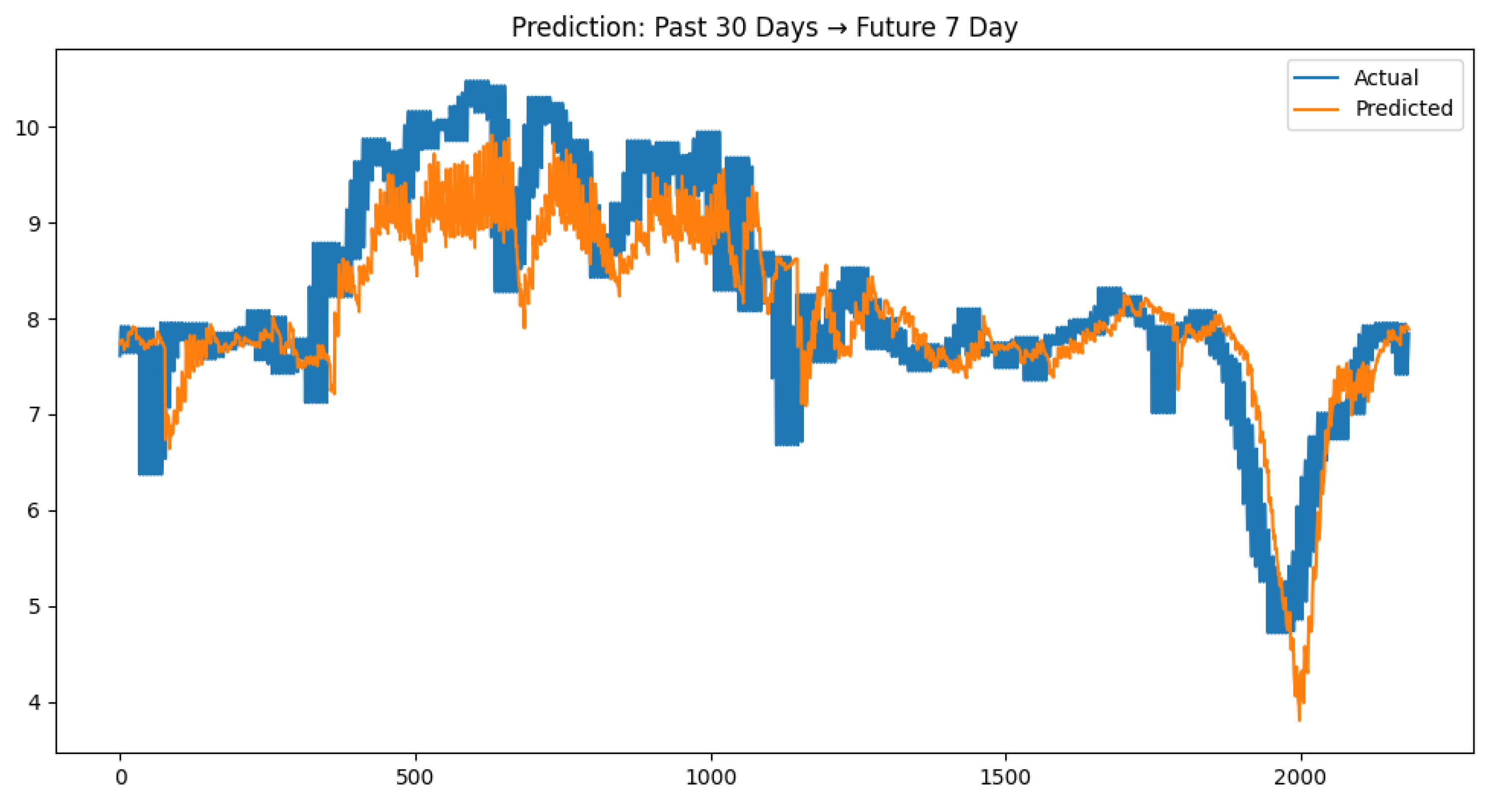
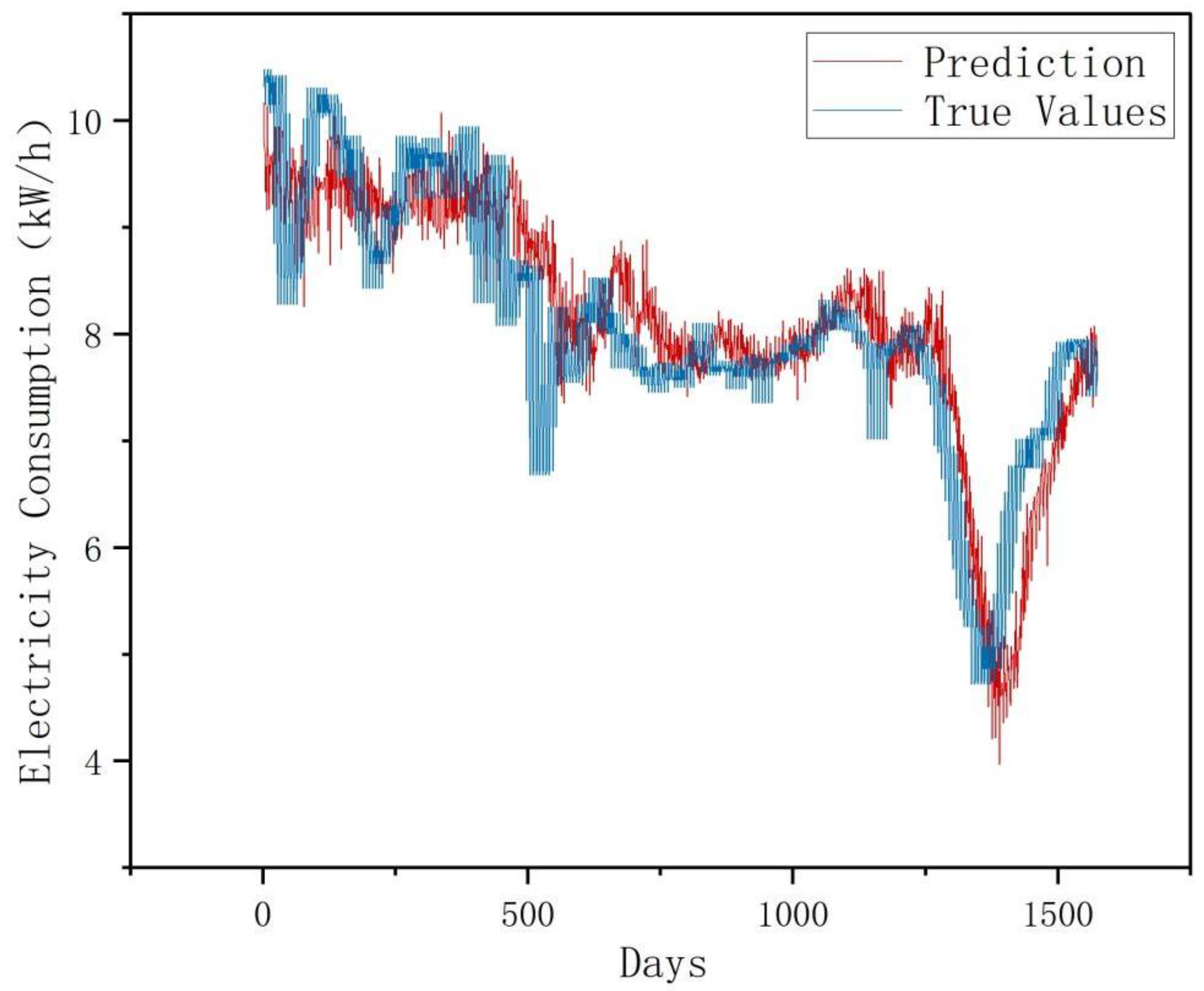
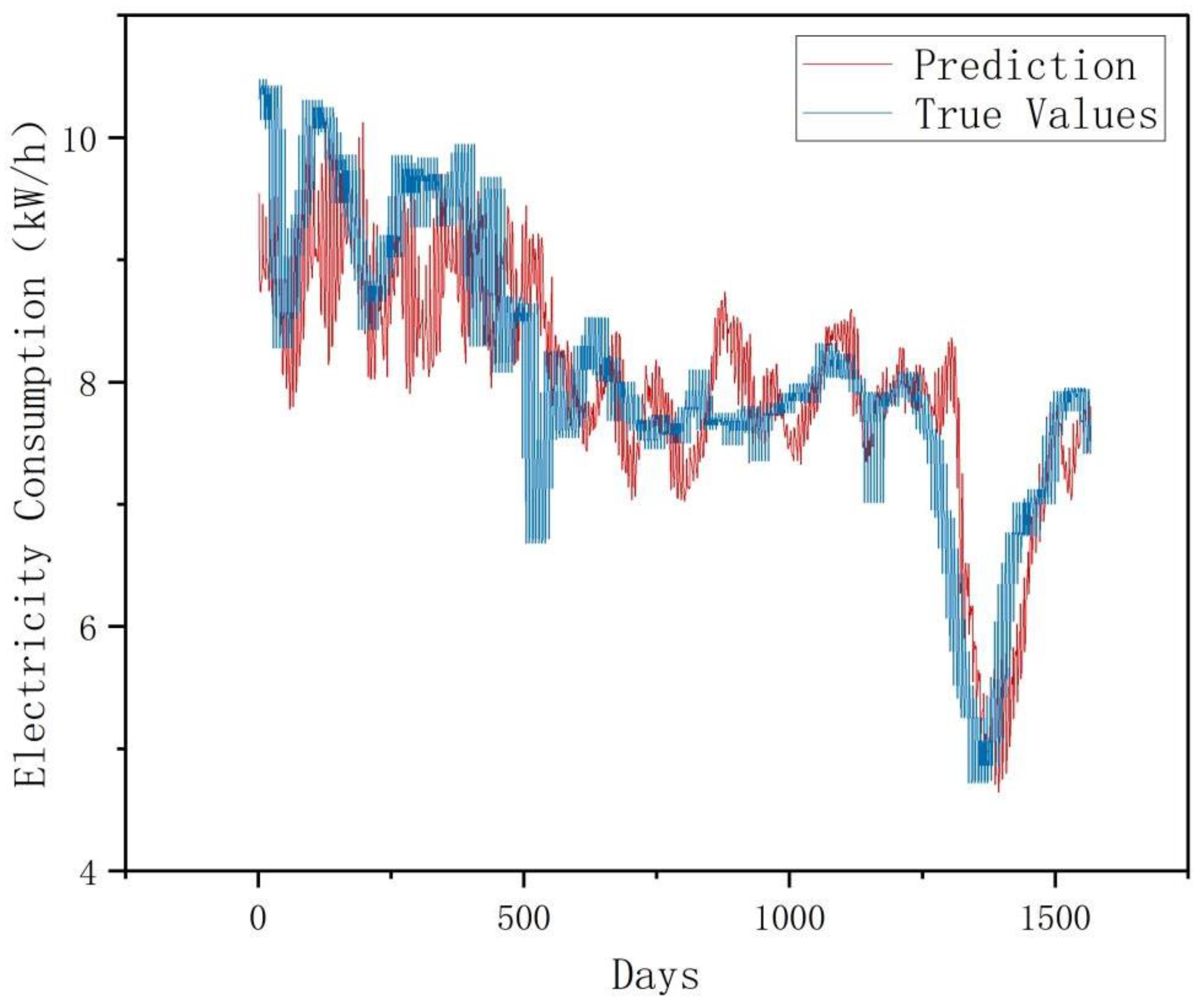
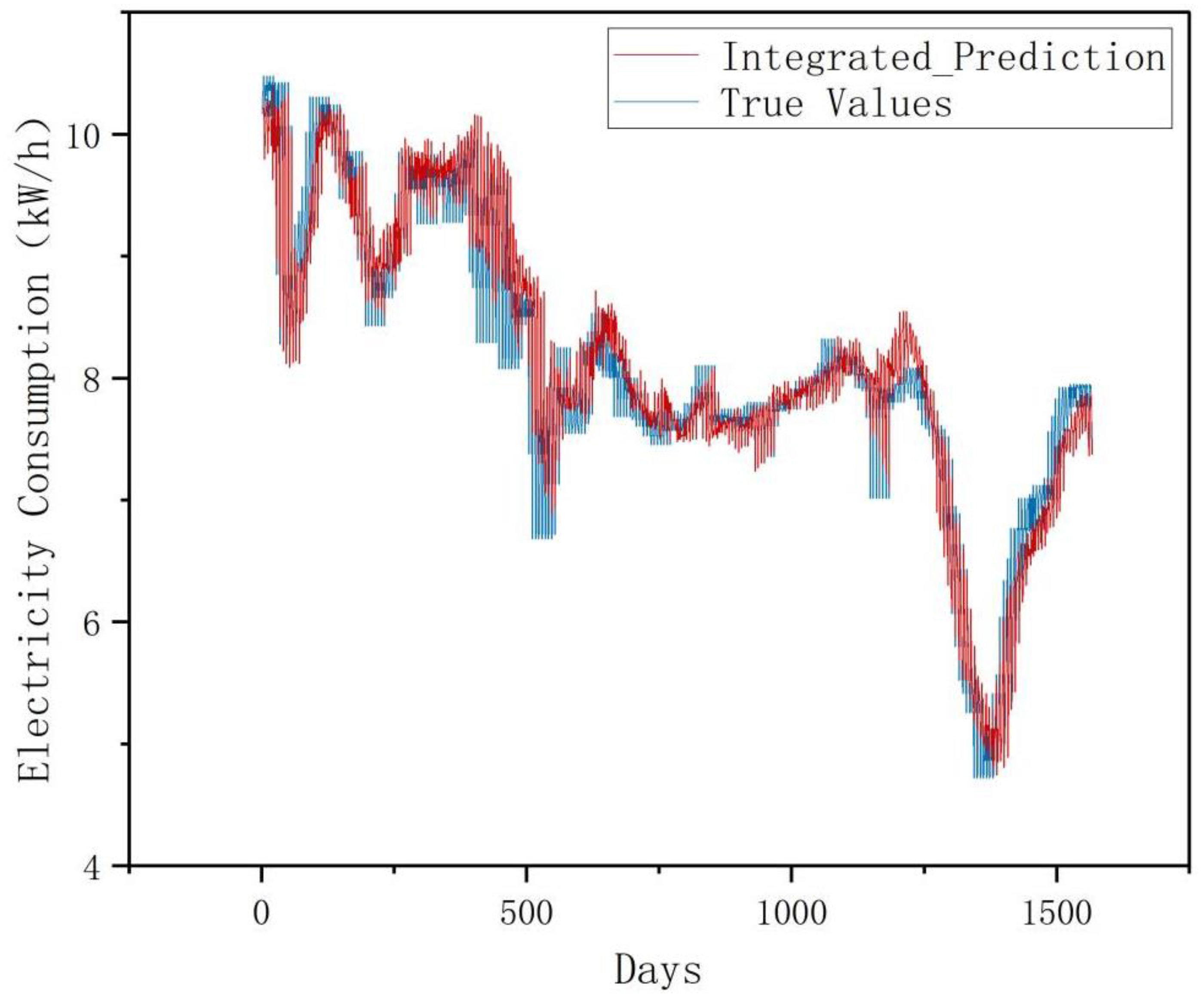
This experiment employs a univariate monthly electricity sales forecasting case study, where original data is partitioned into training, validation, and test sets at a 7:1:2 ratio. Models predict 7-day electricity sales using 30-day historical sequences. Four architectures were implemented and validated: LSTM, Informer, RevInformer, and VMD-RevInformer. Based on multiple experimental trials calculating indicator means, the predictive performance comparison between various models and actual values is depicted in Figure 6, Figure 7, Figure 8 and Figure 9. As opposed to the LSTM and Informer models, our proposed RevInformer model demonstrates significantly better alignment with actual values in predicting the target data, achieving prediction outcomes closest to the ground truth.

To further compare predictive accuracy, five performance metrics rigorously evaluate model efficacy: MAE, MSE, RMSE, MAPE and MSPE. MAE quantifies the average absolute deviation between predictions and true values, particularly effective for regularly distributed errors; MSE and RMSE demonstrate heightened sensitivity to larger errors due to their quadratic nature; MAPE and MSPE measure relative deviation through percentage-based scaling. Lower values across all metrics indicate stronger predictive capability, with optimal performance approaching zero. Comprehensive quantitative results are detailed in the following table:

Table 4. Performance Benchmarking: LSTM vs. Informer vs. RevInformer vs. VMD-RevInformer.

	MSE	MAE	RMSE	MAPE（%）	MSPE(%)
LSTM	0.506737	0.469673	0.685327	6.416559	0.813309
Informer	0.457568	0.456091	0.622173	5.985666	0.721323
RevInformer	0.387774	0.375074	0.612433	5.594999	0.625999
VMD-RevInformer	0.155937	0.044783	0.211621	1.986559	0.074951

Table 4. Performance Benchmarking: LSTM vs. Informer vs. RevInformer vs. VMD-RevInformer.

	MSE	MAE	RMSE	MAPE（%）	MSPE(%)
LSTM	0.506737	0.469673	0.685327	6.416559	0.813309
Informer	0.457568	0.456091	0.622173	5.985666	0.721323
RevInformer	0.387774	0.375074	0.612433	5.594999	0.625999
VMD-RevInformer	0.155937	0.044783	0.211621	1.986559	0.074951

Tabular results confirm that for long-term time-series forecasting, Informer surpasses LSTM across key metrics including MSE, MAE, and RMSE. The enhanced RevInformer further elevates performance, achieving the lowest MSE (0.3878—23.5% lower than LSTM and 15.3% lower than Informer), optimal MAE (0.3751, representing a 17.8% reduction versus the suboptimal Informer), and minimal MAPE (5.595%, 12.8% lower than LSTM). These results demonstrate RevInformer’s inherent superiority in training and forecasting capabilities.

Integration with VMD preprocessing yields transformative improvements in error suppression and stability: MAE decreases by nearly 90.5% compared to standalone RevInformer (compressing absolute error to one-tenth of its original magnitude), MSPE declines by 88.2% (significantly mitigating outlier interference), and RMSE drops by 65.4% (effectively controlling prediction instability). The consistent optimization across all metrics indicates that VMD reduces model learning complexity while synergizing with RevInformer’s reverse-propagation gradient architecture. Critically, although the base RevInformer already excels among non-enhanced models, VMD provides complementary enhancements across all indicators, proving that signal decomposition remains effective even for advanced architectures. This establishes the VMD-RevInformer framework as the preferred solution for high-precision temporal forecasting tasks.

4.4. Contribution of Each Module

To elucidate the specific contributions of the proposed method’s innovative components (VMD and RevInformer), a series of ablation studies with quantitative attribution analysis was conducted. As detailed in Table 6, three key comparative configurations were implemented:

1)

Baseline: Original Informer model;

2)

VMD-Informer: Baseline enhanced with Variational Mode Decomposition (VMD) for data preprocessing;

3)

VMD-RevInformer: VMD-Informer with its core module replaced by the proposed RevInformer.

Experiments utilized a univariate electricity sales dataset, with primary evaluation metrics including MSE, MAE, RMSE, MAPE and MSPE.

Table 5. Comparative Evaluation of Innovative Modules.

	MSE	MAE	RMSE	MAPE（%）	MSPE (%)
Informer	0.506737	0.469673	0.685327	6.416559	0.813309
VMD-Informer	0.155937	0.165839	0.220879	2.066998	0.075588
VMD-RevInformer	0.048788	0.044783	0.211621	1.986559	0.074951

Table 5. Comparative Evaluation of Innovative Modules.

	MSE	MAE	RMSE	MAPE（%）	MSPE (%)
Informer	0.506737	0.469673	0.685327	6.416559	0.813309
VMD-Informer	0.155937	0.165839	0.220879	2.066998	0.075588
VMD-RevInformer	0.048788	0.044783	0.211621	1.986559	0.074951

The tabulated results reveal that incorporating the VMD module for data preprocessing yields exceptionally significant performance gains across all evaluation metrics compared to the baseline Informer. Specifically, MSE decreases by approximately 90.4% and MSPE by 90.7%, strongly demonstrating that VMD is the core driver for enhancing forecasting precision. This module effectively addresses nonlinearity and non-stationarity in univariate electricity sales data, substantially optimizing input data quality and reducing overall prediction errors.

When replacing the core forecasting module from Informer to RevInformer atop VMD preprocessing, while MSE exhibits a marginal increase versus VMD-Informer, other critical metrics—MAE, MAPE, and MSPE—show marked improvements: MAE reduction of ~73.0% (achieving the lowest recorded value for this metric), MAPE reduction of ~3.9%. The RevInformer module delivers critical refinements, indicating its architectural superiority in modeling complex temporal dependencies. It proves particularly effective at reducing outliers or large deviations in predictions, aligning model outputs more closely with the central tendency of actual value sequences.

The ablation experiments demonstrate that the performance enhancement of the proposed method stems from the synergistic interplay between both modules: The VMD module, acting as a robust data preprocessing mechanism, delivers dominant contributions to overall prediction accuracy and stability, playing a decisive role in reducing all categories of error metrics. As an enhanced core forecasting architecture, the RevInformer module complements this foundation by providing targeted refinements to prediction robustness and consistency through its specialized structural design.

5. Conclusion and Future Work

This study addresses the challenges of abruptness, stochasticity, and complexity in monthly electricity sales forecasting, along with existing methods’ limitations in handling long-sequence time series data. We propose RevInformer, an enhanced Transformer-based model, integrated with Variational Mode Decomposition (VMD) optimized via Zebra Optimization Algorithm (ZOA) for data processing. The superiority of this approach is demonstrated through five key evaluation metrics in comparative studies with existing forecasting methods. Results indicate that our model achieves approximately 70% error reduction across all metrics compared to LSTM predictions, with MSPE improvement reaching approximately 90%. Relative to the Informer model, it delivers an average 65% optimization in error metrics. When benchmarked against the RevInformer model without VMD-processed raw data, our method demonstrates performance enhancements ranging from 64% to 88%.

The comparative results demonstrate that:

1)

Input data processed through VMD are decomposed into distinct Intrinsic Mode Functions (IMFs), where the shortened sequences substantially alleviate computational burden while significantly enhancing individual IMF forecasting precision. This reveals the feasibility of integrating signal decomposition with deep learning architectures, offering a novel approach to complex time series prediction;

2)

The incorporation of reversible layers into the Informer framework effectively addresses distribution shift in temporal data, enabling bidirectional propagation with parameter sharing to reduce memory consumption. Simultaneously, the Probsparse self-attention mechanism lowers computational complexity, while the generative inference decoder permits single-step prediction sequence generation, collectively optimizing forecasting efficiency.

Experimental results demonstrate that while the RevInformer model exhibits significant potential for electricity consumption forecasting across extended time horizons, its direct application to raw sequences reveals inherent limitations in decoupling non-stationary, multi-scale characteristics. The VMD preprocessing effectively mitigates RevInformer’s frequency-domain decoupling deficiency, and future research will focus on advancing hybrid methodologies that integrate signal processing theory with large-scale predictive models to address complex temporal forecasting challenges.

References

- H. Dong, J. Zhu, S. Li, Y. Miao, C. Y. Chung, and Z. Chen, “Probabilistic Residential Load Forecasting with Sequence-to-Sequence Adversarial Domain Adaptation Networks,” J. Mod. Power Syst. Clean Energy, vol. 12, no. 5, pp. 1559–1571, Sept. 2024. [CrossRef]
- R. Smith, K. Meng, Z. Dong, and R. Simpson, “Demand response: a strategy to address residential air-conditioning peak load in Australia,” J. Mod. Power Syst. Clean Energy, vol. 1, no. 3, pp. 219–226, Dec. 2013. [CrossRef]
- X. Sun et al., “Electricity Theft Detection Method Based on Ensemble Learning and Prototype Learning,” J. Mod. Power Syst. Clean Energy, vol. 12, no. 1, pp. 213–224, Jan. 2024. [CrossRef]
- H. Gong and H. Xing, “Predicting the highest and lowest stock price indices: A combined BiLSTM-SAM-TCN deep learning model based on re-decomposition,” Appl. Soft Comput., vol. 167, p. 112393, Dec. 2024. [CrossRef]
- G. Box, “Box and Jenkins: Time Series Analysis, Forecasting and Control,” in A Very British Affair, London: Palgrave Macmillan UK, 2013, pp. 161–215. [CrossRef]
- W. Zhong et al., “Accurate and efficient daily carbon emission forecasting based on improved ARIMA,” Appl. Energy, vol. 376, p. 124232, Dec. 2024. [CrossRef]
- L. Ouyang, F. Zhu, G. Xiong, H. Zhao, F. Wang, and T. Liu, “Short-term traffic flow forecasting based on wavelet transform and neural network,” in 2017 IEEE 20th International Conference on Intelligent Transportation Systems (ITSC), Oct. 2017, pp. 1–6. [CrossRef]
- D. Gordon, L. Breiman, J. H. Friedman, R. A. Olshen, and C. J. Stone, “Classification and Regression Trees.,” Biometrics, vol. 40, no. 3, p. 874, Sept. 1984. [CrossRef]
- T. K. Ho, “Random decision forests,” in Proceedings of 3rd International Conference on Document Analysis and Recognition, Aug. 1995, pp. 278–282 vol.1. [CrossRef]
- M. I. Jordan et al., “SERIAL ORDER: A PARALLEL DISTRmUTED PROCESSING APPROACH,” 2009. Accessed: Aug. 08, 2025. [Online]. Available: https://www.semanticscholar.org/paper/SERIAL-ORDER%3A-A-PARALLEL-DISTRmUTED-PROCESSING-Jordan-Conway/f8d77bb8da085ec419866e0f87e4efc2577b6141?p2df.
- J. L. Elman, “Finding structure in time,” Cogn. Sci., vol. 14, no. 2, pp. 179–211, Apr. 1990. [CrossRef]
- N.-T. Bui et al., “TSRNet: Simple Framework for Real-time ECG Anomaly Detection with Multimodal Time and Spectrogram Restoration Network,” Mar. 05, 2024, arXiv: arXiv:2312.10187. [CrossRef]
- S. Hochreiter and J. Schmidhuber, “Long short-term memory,” Neural Comput., vol. 9, no. 8, pp. 1735–1780, Nov. 1997. [CrossRef]
- F. A. Gers, J. Schmidhuber, and F. Cummins, “Learning to forget: continual prediction with LSTM,” in 1999 Ninth International Conference on Artificial Neural Networks ICANN 99. (Conf. Publ. No. 470), Sept. 1999, pp. 850–855 vol.2. [CrossRef]
- Y. Lecun, L. Bottou, Y. Bengio, and P. Haffner, “Gradient-based learning applied to document recognition,” Proc. IEEE, vol. 86, no. 11, pp. 2278–2324, Nov. 1998. [CrossRef]
- A. Vaswani et al., “Attention Is All You Need,” Aug. 02, 2023, arXiv: arXiv:1706.03762. [CrossRef]
- J. Zhu, D. Liu, H. Chen, J. Liu, and Z. Tao, “DTSFormer: Decoupled temporal-spatial diffusion transformer for enhanced long-term time series forecasting,” Knowl.-Based Syst., vol. 309, p. 112828, Jan. 2025. [CrossRef]
- T. Zhou, Z. Ma, Q. Wen, X. Wang, L. Sun, and R. Jin, “FEDformer: Frequency Enhanced Decomposed Transformer for Long-term Series Forecasting,” June 16, 2022, arXiv: arXiv:2201.12740. [CrossRef]
- H. Zhou et al., “Informer: Beyond Efficient Transformer for Long Sequence Time-Series Forecasting,” Proc. AAAI Conf. Artif. Intell., vol. 35, no. 12, Art. no. 12, May 2021. [CrossRef]
- W. Yu, Y. Dai, T. Ren, and M. Leng, “Short-time photovoltaic power forecasting based on Informer model integrating Attention Mechanism,” Appl. Soft Comput., vol. 178, p. 113345, June 2025. [CrossRef]
- J.-C. Li, L.-P. Sun, X. Wu, and C. Tao, “Enhancing financial time series forecasting with hybrid Deep Learning: CEEMDAN-Informer-LSTM model,” Appl. Soft Comput., vol. 177, p. 113241, June 2025. [CrossRef]
- Huang, T. Zhao, D. Huang, B. Cen, Q. Zhou, and W. Chen, “Artificial intelligence-based power market price prediction in smart renewable energy systems: Combining prophet and transformer models,” Heliyon, vol. 10, no. 20, p. e38227, Oct. 2024. [Google Scholar] [CrossRef]
- G. Zhang, B. Xu, H. Liu, J. Hou, and J. Zhang, “Wind Power Prediction Based on Variational Mode Decomposition and Feature Selection,” J. Mod. Power Syst. Clean Energy, vol. 9, no. 6, pp. 1520–1529, Nov. 2021. [CrossRef]
- Y. Cai, Z. Tang, and Y. Chen, “Can real-time investor sentiment help predict the high-frequency stock returns? Evidence from a mixed-frequency-rolling decomposition forecasting method,” North Am. J. Econ. Finance, vol. 72, p. 102147, May 2024. [CrossRef]
- “Signal processing for miniature mass spectrometer based on LSTM-EEMD feature digging,” Talanta, vol. 281, p. 126904, Jan. 2025. [CrossRef]
- T. Kim, J. Kim, Y. Tae, C. Park, J.-H. Choi, and J. Choo, “Reversible Instance Normalization for Accurate Time-Series Forecasting against Distribution Shift,” presented at the International Conference on Learning Representations, Oct. 2021. Accessed: Aug. 08, 2025. [Online]. Available: https://openreview.net/forum?id=cGDAkQo1C0p.