1. Introduction
The advancement of high-speed air-breathing propulsion systems is a cornerstone for the future of aerospace transportation, with applications ranging from supersonic transport to hypersonic cruise vehicles [
1]. Central to the performance of these systems is the supersonic inlet, a critical component tasked with capturing freestream air and efficiently decelerating it to subsonic conditions suitable for the engine compressor [
2]. The historical context of these systems reveals the persistent design challenges that motivate ongoing research [
3]. This deceleration process is achieved through a carefully managed system of shock waves; however, the interaction of these strong shocks with the boundary layers developing on the intake surfaces presents one of the most significant challenges in high-speed flight. This phenomenon, known as shock/boundary layer interaction (SBLI), subjects the low-momentum fluid near the wall to a severe adverse pressure gradient, which can provoke a range of detrimental effects [
4]. These consequences include a rapid thickening of the boundary layer, increased total pressure losses, and, in severe cases, large-scale flow separation [
5,
6]. The resulting non-uniform flow delivered to the engine, formally quantified as flow distortion, is a primary driver of reduced engine performance and stability, as outlined by industry guidelines. At its most extreme, SBLI can lead to a catastrophic event known as “inlet unstart,” where the shock system is violently expelled, causing an abrupt loss of thrust and posing a significant risk to the vehicle. Therefore, the effective management and control of SBLI are paramount for robust and reliable inlet operation [
7].
Over several decades, various flow control strategies have been developed to mitigate SBLI, with boundary layer bleed being one of the most mature and widely implemented techniques [
8]. This method involves the removal of the low-energy, near-wall fluid through porous surfaces, slots, or discrete holes located in the interaction region, a concept proven effective in both fundamental studies and practical applications [
9,
10]. By removing this fluid, the boundary layer becomes more resilient to the adverse pressure gradient, which can effectively suppress flow separation, stabilize the terminal shock position, and improve pressure recovery (
PR), forming an integral part of high-speed design philosophies [
11].
Despite its benefits for SBLI control, the implementation of a bleed system introduces its own set of complex fluid dynamics consequences. The act of suction through discrete geometries can induce powerful secondary flows and tangential velocity components within the main duct flow. This generates a rotational, non-axial flow field at the engine face, a condition known as swirl [
12]. The criticality of this issue is underscored by the aerospace industry’s development of standardized methodologies, such as SAE AIR5686, for the explicit purpose of quantifying swirl distortion as a key performance metric [
13]. It is well-established that such rotational flow can negatively impact engine stability by altering the incidence angles on compressor blades, potentially leading to reduced efficiency, increased structural loads, and a diminished stall margin [
14]. Indeed, the practical characterization of swirl in high-speed inlets has been the focus of dedicated experimental and numerical efforts [
15]. While previous work has identified bleed as a source of vorticity, a systematic and parametric investigation that quantitatively links the bleed rate required for SBLI control to the resulting swirl intensity (
SI) across a range of flight conditions has not been fully explored.
This study aims to address this gap through a parametric numerical investigation of a bleed-enabled external compression supersonic intake. The primary objective is to establish a quantitative relationship between the freestream Mach number, the applied bleed rate for effective SBLI control, and the consequential swirl and pressure distortion metrics at the aerodynamic interface plane (AIP). Comprehensive three-dimensional, steady-state Reynolds-Averaged Navier–Stokes (RANS) based Computational Fluid Dynamics (CFD) simulations for a single-ramp supersonic intake model are performed for a range of freestream Mach numbers (M∞ = 1.4-1.9), and the results are discussed in terms of relationships of SBLI, pressure recovery and swirl characteristics of the intake flow field with and without bleed system.
2. Methodology and Model Geometry
The results are obtained from three-dimensional, steady-state RANS simulations of a single-ramp, external compression supersonic inlet, evaluated with bleed (WB) and without bleed (WOB) system. The computational model, model geometry, computational grid, test matrix and boundary conditions, and post-processing methodology are described below.
2.1. Computational Methodology
The CFD simulations are performed by using ANSYS Fluent 2017 CFD software by solving the 3-D, steady-state, compressible RANS equations with the total energy equation. Air is treated as an ideal gas with temperature-dependent properties (Sutherland-law viscosity; temperature-dependent thermal conductivity). Turbulence is modeled with the realizable
k–ε model and enhanced wall treatment (EWT), which is appropriate for adverse pressure gradient flow with shock/boundary layer interaction and local separation. A pressure-based coupled solver is used in double precision. Gradients are computed with least-squares cell-based method; second-order method is used for pressure interpolation; second-order upwind method is used for production iterations for momentum, energy,
k, and
ε. A short first-order pass is used only to stabilize initial shock formation before switching to second order. The Courant number is ramped from ≈1 to ≈30 as residuals settle; the pseudo-transient option is not used. Under-relaxation factors are staged from start-up (pressure = 0.5,
k = 0.2,
ε = 0.2, momentum = 0.5, energy = 0.5) to production (pressure = 0.8-0.9,
k = 0.7,
ε = 0.7, momentum = 0.9, energy = 0.9). Algebraic multigrid is employed with default cycling; temperature and pressure-coupled smoothing are set to 0.1/0.7. Full multigrid (FMG) initialization is performed from the pressure far-field. Convergence is declared when all scaled residuals fall below 1 x 10
−5 and the global mass imbalance is ≤ 0.1% [
16].
2.2. Model Geometry and Computational Domain
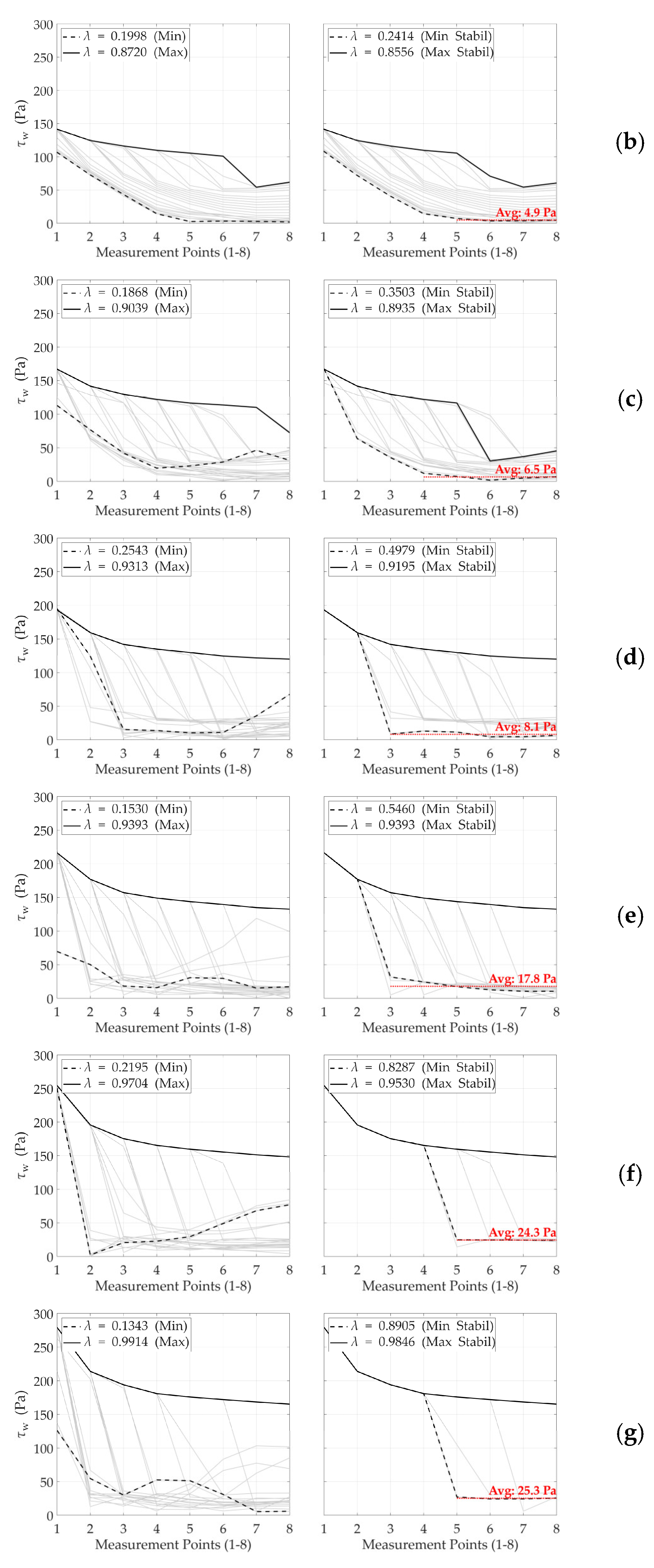
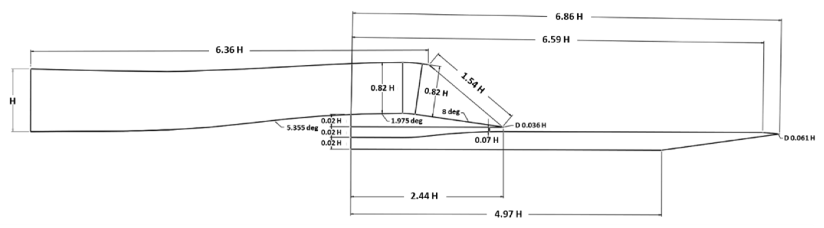
The model is a single-ramp external compression supersonic inlet geometry with a ramp angle of 8°, followed by a short diffuser and an Aerodynamic Interface Plane (AIP), as shown in
Figure 1.
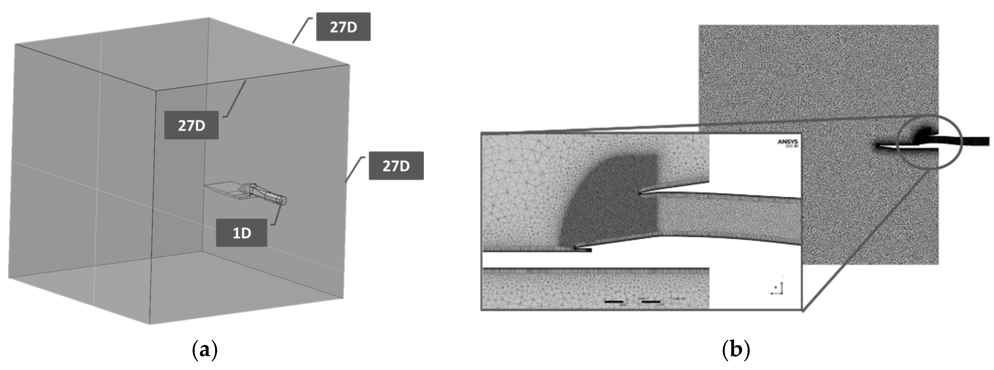
The external flow rectangular computational domain, as shown in
Figure 2, is a Cartesian box with a size of 27 D x 27 D x 27 D to avoid boundary interference with the upstream, downstream, and all lateral boundaries placed away from the inlet duct which has a reference diameter D (= H).
2.3. Grid Independence Study
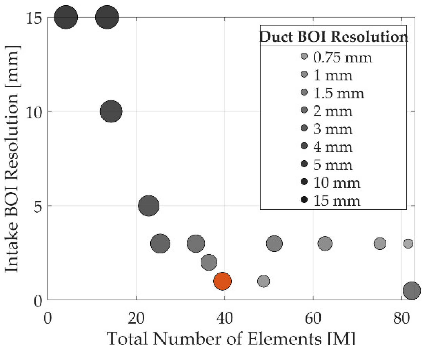
To ensure that the numerical results are independent of the spatial discretization and to quantify the numerical uncertainty, a comprehensive grid independence study is conducted. The primary objective of this study is to identify a grid configuration that provides a sufficient level of accuracy for capturing the key flow phenomena, such as shock waves, shock–boundary-layer interactions, and flow separation, while maintaining a manageable computational cost. A systematic approach is adopted where several key meshing parameters are varied to generate a series of grids with a wide range of element counts, from approximately 1.5 million to nearly 83 million cells.
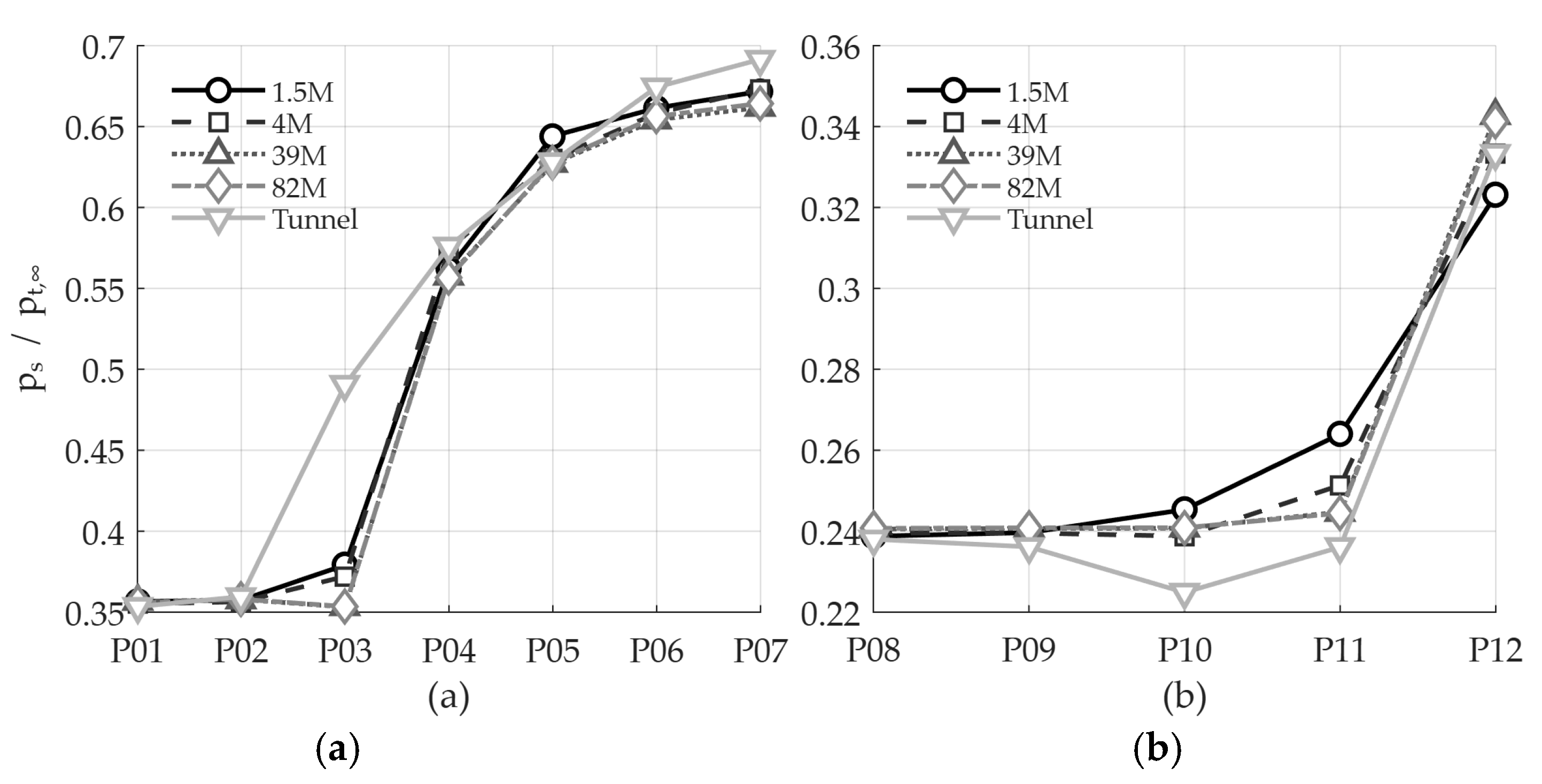
The parameters investigated include: the resolution of local refinement regions using Bodies of Influence (BOI) in the intake and duct sections, the inflation layer properties (first cell thickness, number of layers, and growth rate), and the general surface and body sizing of the computational domain. The independence of the solution is assessed by comparing the static pressure ratio (ps / pt,∞) distributions along the compression surface and the splitter plate for each grid configuration against the experimental wind tunnel data.
The effect of the various meshing parameters investigated as part of the grid independence study on the total number of elements (computational cost) is visualized in the grid-parameter map in
Figure 3. In this chart, the
x-axis represents the total number of elements, while the
y-axis shows the Intake BOI resolution, which is critical for capturing the shock structures. The color of the bubbles encodes the Duct BOI resolution, and their size represents the surface (intake surface) mesh sizing. The chart quantitatively demonstrates that refining the resolution in the BOI regions (a smaller mm value) significantly increases the total number of elements. The reference grid, highlighted in orange with approximately 39 million elements, is selected based on the observation that the pressure ratio shown in
Figure 4.
Figure 4 shows that the pressure distributions converge with grid refinement and that the 39 M and 82 M solutions are essentially indistinguishable across both surfaces. On the compression surface (P01-P07, panel a), all grids reproduce the gradual rise from P01-P02 and the sharp increase through P03-P05 associated with the ramp SBLI, with the fine grids capturing the post-ramp plateau beyond P05. On the splitter plate (P08-P12, panel b), the fine grids also collapse, recovering the local minimum around P10 and the subsequent rise toward P12. Differences to the tunnel data appear mainly near P03-P04, P10 and P12 stations that are highly sensitive to boundary layer state and local SBLI/corner interactions, whereas the remainder of the taps show good agreement. Taken together, these results indicate that further refinement beyond ~39 M cells brings negligible improvement to the local pressure field, supporting the selection of the 39 M grid for production runs.
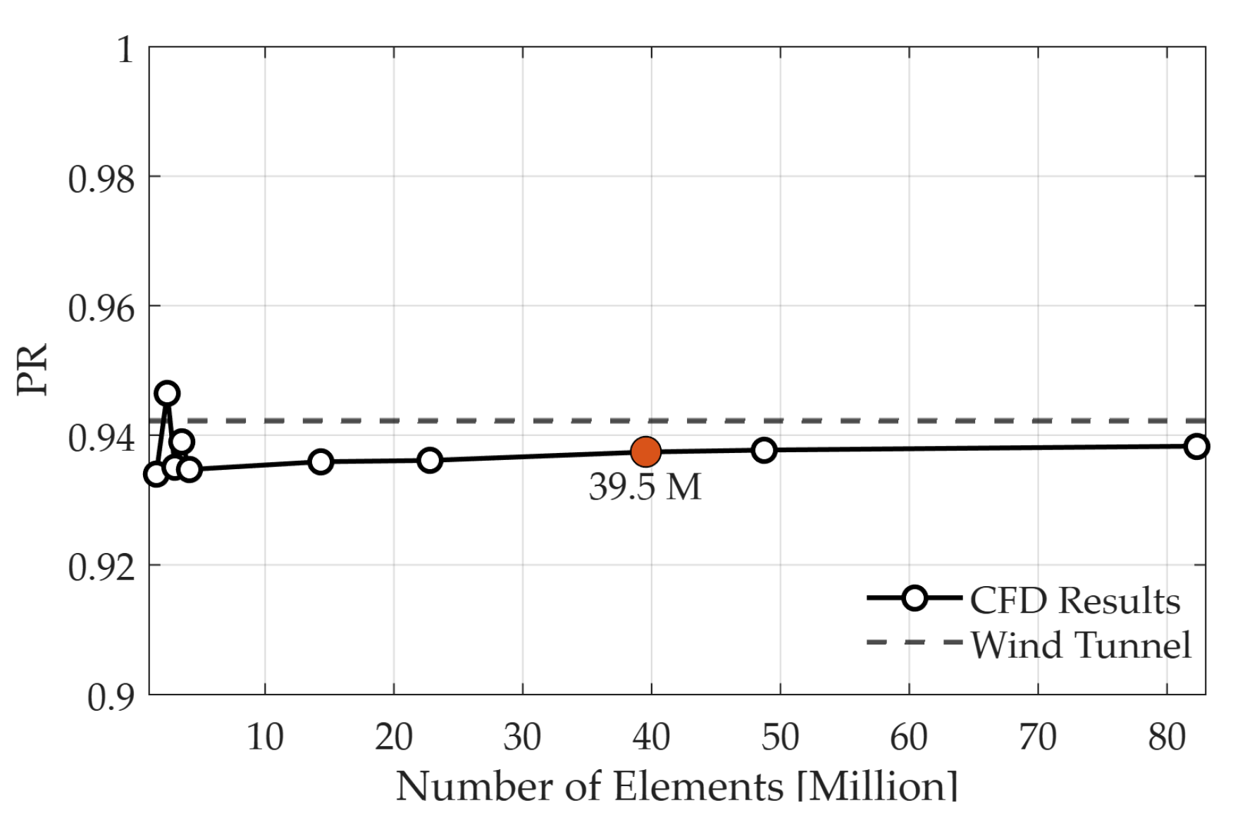
In addition to the local static pressure comparisons, the grid independence of a key global performance metric, the
PR at the AIP, is assessed in
Figure 5. This analysis is performed at the reference operating condition at M
∞ = 1.8 and
λ = 0.97. The figure plots the calculated
PR value as a function of the total number of mesh elements for ten different grid configurations. The corresponding experimental value from the wind tunnel test is also shown as a dashed line for reference. The results show a clear trend of convergence as the mesh is refined. For coarser grids with fewer than 10 million elements, the calculated
PR is highly sensitive to the mesh resolution. As the element count increases, the
PR value asymptotically approaches a stable value. The curve visibly flattens for meshes beyond approximately 40 million elements, with the difference in
PR between the 40 M and 82 M grids being negligible.
2.4. Test Matrix and Boundary Conditions
The operating condition (operating-map) is parameterized by the flow ratio,
λ:
where,
Ac is the geometric cowl capture area, and
A0 is the equivalent capture area. For each freestream Mach number, the traverse is carried out from supercritical through critical into subcritical conditions until the last stable point (buzz onset) is reached. At every operating point, the following performance parameters are evaluated and reported: pressure recovery (
PR), swirl angle (
α), swirl intensity (
SI) (ring-wise) at the AIP, and the mass-averaged total-pressure loss factor (
ϵloss).
This study is designed to systematically investigate the effects of freestream Mach number and bleed rate on the SBLI phenomena and the resulting engine-face flow quality metrics, including
PR and swirl. To achieve this, a comprehensive case matrix is established, encompassing a range of operating conditions. The two primary parameters varied in this study are the M
∞ and the bleed configurations: WB and WOB. The analyses are conducted at three distinct Mach numbers: M
∞ = 1.6, 1.8, and 1.9. For each Mach number, a baseline WOB configuration is simulated to serve as a reference against a WB configuration. The WB configuration is implemented via a porous-jump boundary condition fitted to hole-resolved 3-D RANS [
18]. The viscous (
F1) and inertial (
F2) resistances are expressed via a quadratic of pressure drop (
∆p) versus exit-plane superficial velocity (
V), parameterized by porosity, length-to-diameter ratio (
L/D), and hole diameter (
D) [
18]. This model utilizes the optimized geometric parameters determined in a preceding study: for the bleed entry, an
L/D ratio of 1.0 is selected and the porosity level is set to 0.2. For the bleed exit, an
L/D of 0.25 is selected and a porosity of 0.50 is chosen. For all configurations, the back pressure is swept from supercritical through critical into subcritical (unstart) conditions. The complete test matrix, summarizing all simulated conditions, is presented in
Table 1.
2.5. Data Post-Processing and Metric Calculations
This section describes how the AIP data is extracted and how each performance metric is computed. All quantities are evaluated at converged solutions using the same sampling layout and averaging operators to ensure a consistent basis for comparison across the entire case matrix.
The primary metric for intake performance is the total pressure recovery,
PR, which quantifies the efficiency of the pressure-rise process. It is defined as the area-averaged total pressure at the AIP normalized by the freestream total pressure [
2] as:
Total pressure loss factor,
ϵloss, is defined as the difference between the freestream total pressure and the total pressure at the aerodynamic interface plane, normalized by the dynamic pressure at the AIP [
19] as:
where,
γ is the ratio of specific heats, M
AIP is the area average Mach number at the AIP,
ps is the static pressure at the AIP, and
pt,AIP is the total pressure at the AIP.
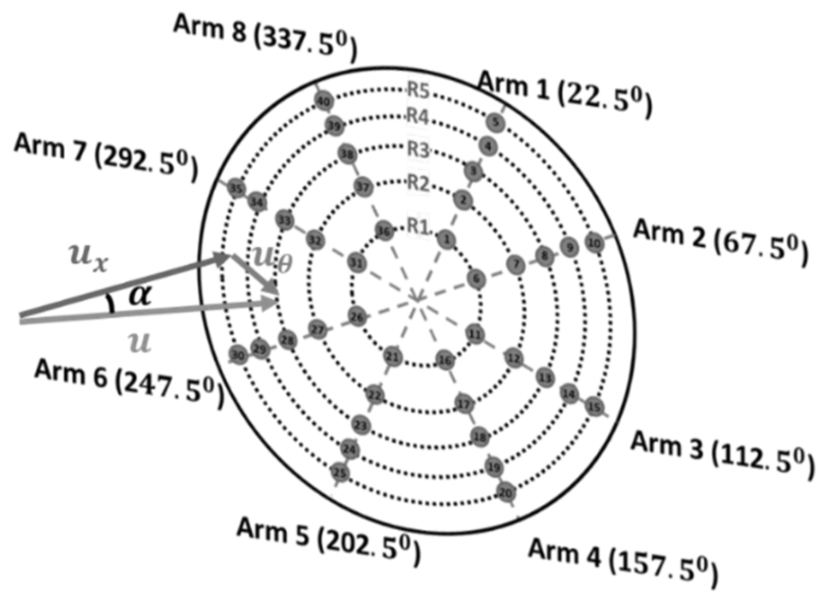
Swirl, or the rotational component of the flow at the engine face, is a critical form of distortion that can significantly affect engine stability. To quantify swirl, the detailed methodology outlined in SAE AIR5686 [
13] is employed. The fundamental metric is the local swirl angle,
αswirl, defined at each point on the AIP, as shown in
Figure 6. It is calculated from the tangential (
uθ) and axial (
ux) velocity components as:
From this local angle, two key SI descriptors are derived to characterize the magnitude and spatial nature of the swirl. The sector swirl intensity (SISA) identifies the maximum absolute mass-flow-averaged swirl angle within any predefined 60-degree sector of the AIP. Similarly, the ring swirl intensity (SIRA) identifies the maximum absolute mass-flow-averaged swirl angle within any of the concentric rings defined at the AIP. These standardized metrics capture the magnitude and spatial nature of the swirl, providing a comprehensive assessment of the rotational distortion delivered to the engine face.
A rake designed to assess the overall pressure at the AIP is depicted in
Figure 6. Eight “arms,” each supporting five evenly spaced pressure ports, are arranged in an 8x5 arrangement, providing 40 measurement locations distributed around the AIP cross section. Any radial or circumferential changes in total pressure that can result from inlet distortions or non-uniformities are captured by this arrangement, which guarantees thorough mapping of the flow field [
20,
21].
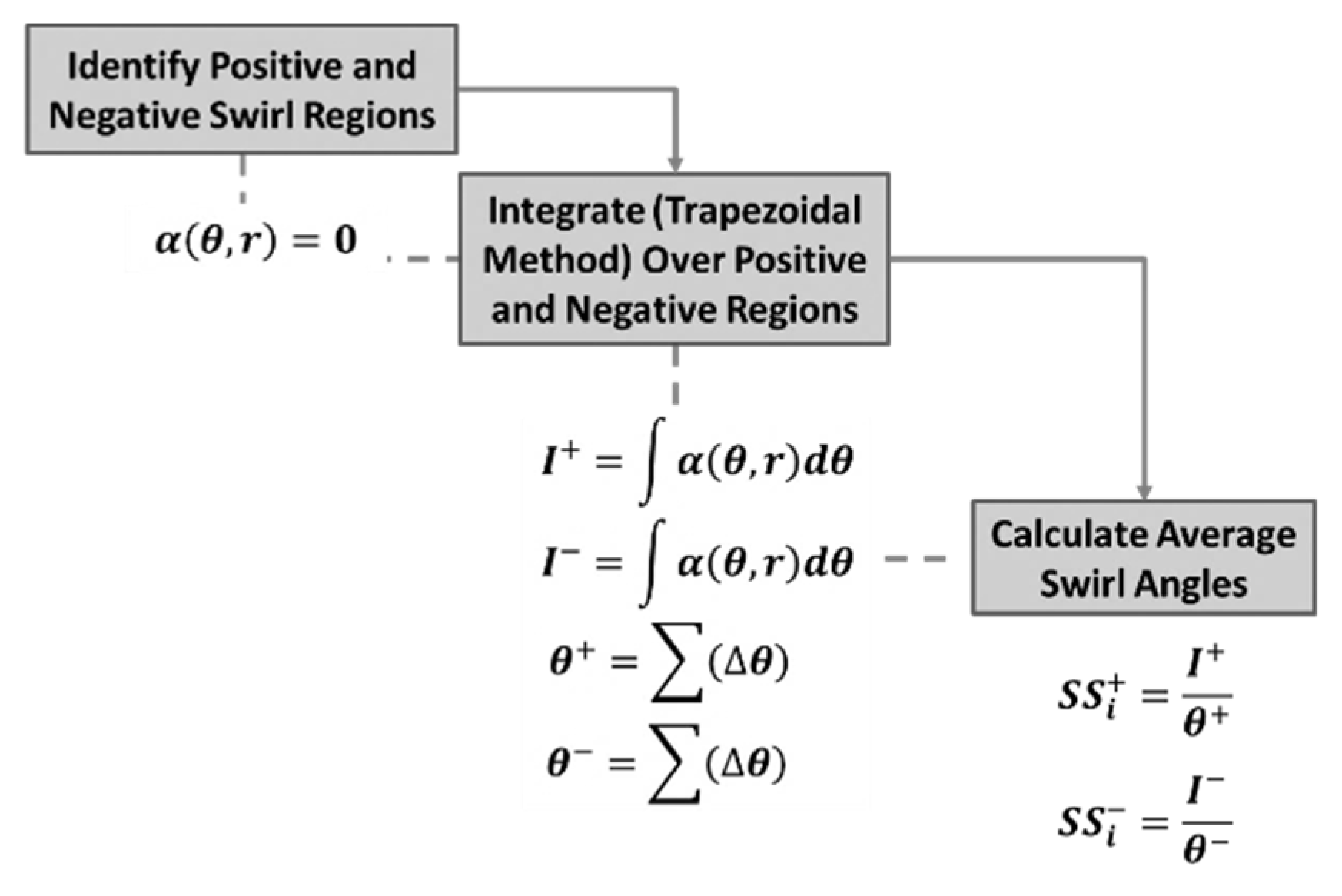
Aside from experimental measurements, the velocity components at the AIP can be recovered using CFD simulations (
Figure 7). The velocity data, specifically the axial,
ux, and tangential,
uθ, components, allow for the determination of swirl parameters including swirl angle,
α(
θ,r), and swirl intensity,
SI at a point
i on the AIP as:
This formula computes a weighted average of the positive and negative swirl sectors, scaled over the full 360° of the ring [
23,
24]. The result is a net
SI for that ring, taking into account both the strength (average angle) and the size (angular extent) of the swirl regions. A high absolute value of
SIi indicates strong swirl distortion, which can affect compressor stability.
3. Results
The results of the CFD simulations are presented and discussed below without and with bleed system for different conditions.
3.1. Intake Characteristic Without Bleed System
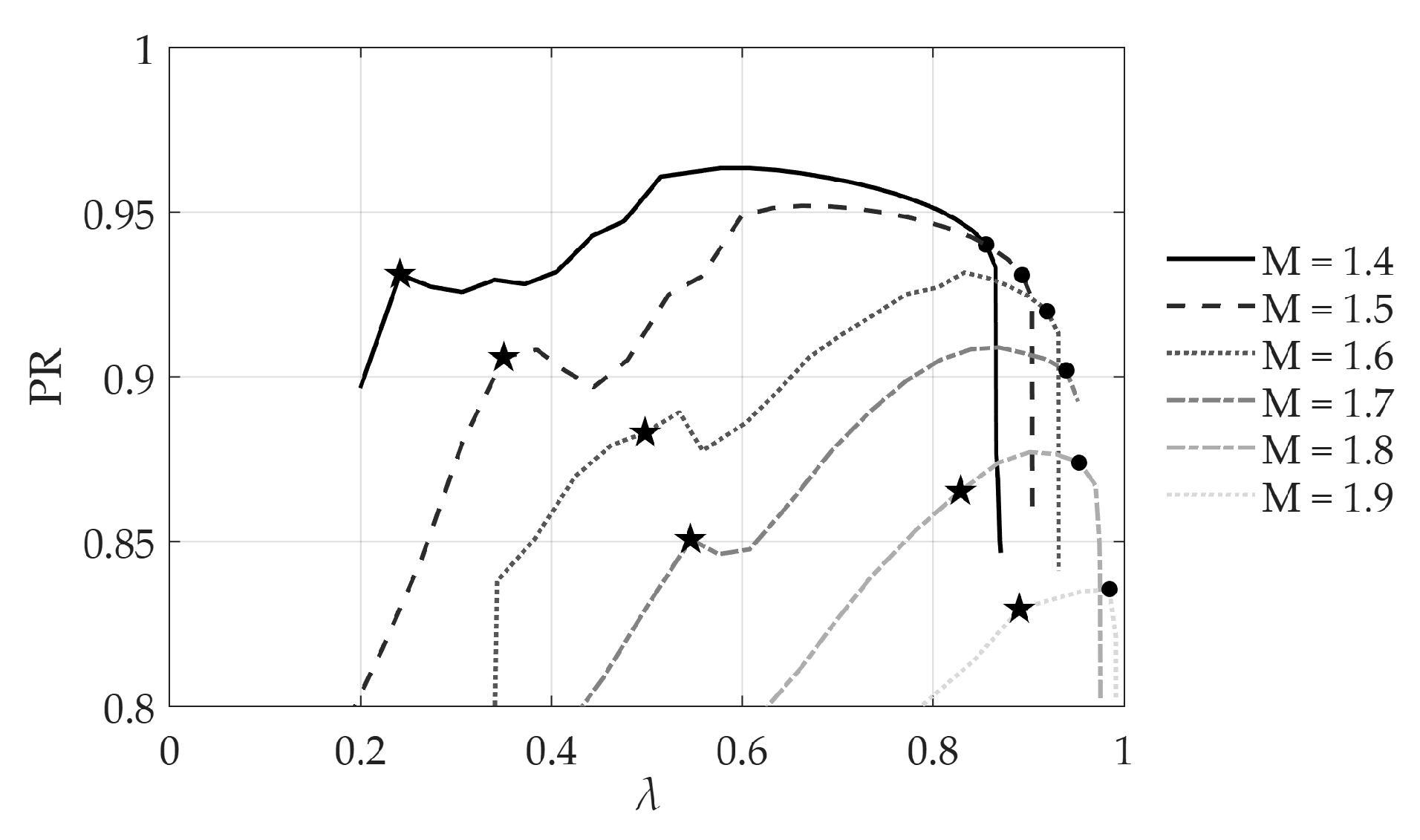
The operational performance map of the inlet is presented for M
∞ ranging from 1.4 to 1.9. In
Figure 8,
PR is plotted against the flow parameter
λ with each line style corresponding to a specific Mach number. This map is crucial for stability assessment, as two critical performance boundaries are explicitly marked on each curve: the star (★) marker indicates the ‘buzz onset’ (the last stable operating point), while the dot (●) marker signifies the ‘throat choking’ condition (the maximum flow or unstart limit). A key trend observed is that as the Mach number increases, the overall peak
PR achieved by the inlet tends to decrease.
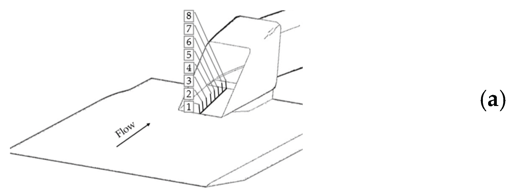
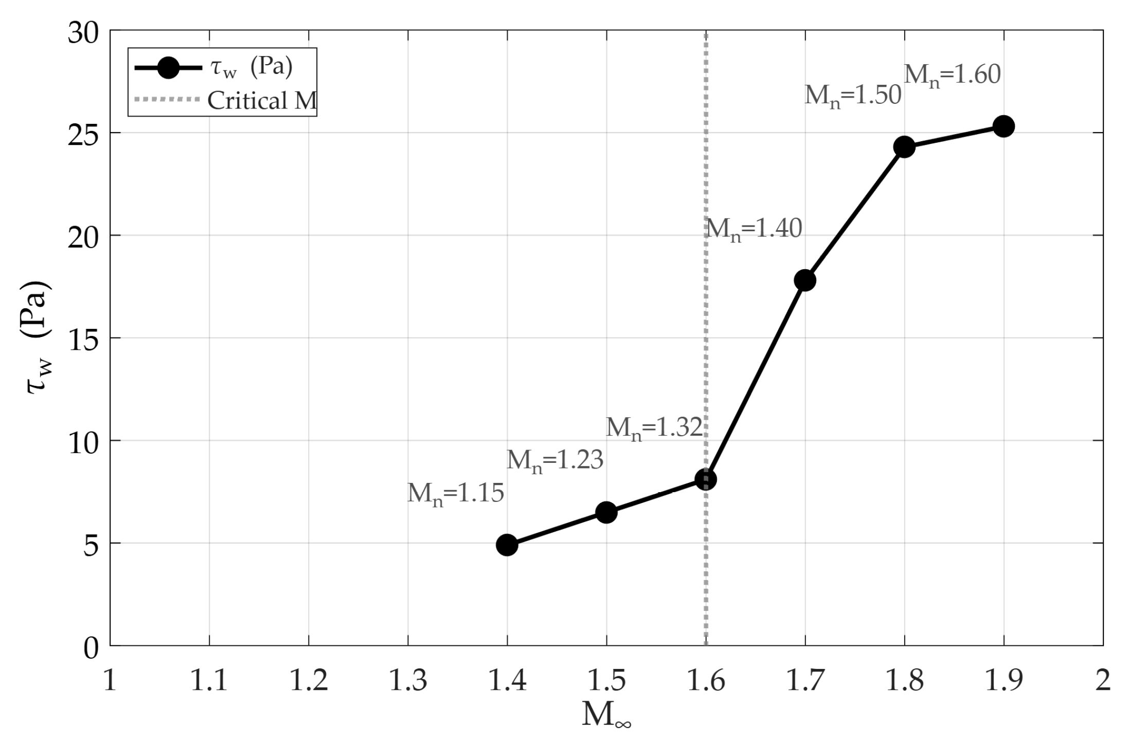
3.2. Wall Shear on Compression Surface
The upstream movement of the terminal shock, as observed in the Mach distributions (
Figure 10), creates a strong adverse pressure gradient. This pressure gradient can cause the boundary layer to separate from the wall, which is the direct cause of the ‘buzz’ instability. To quantify the onset and severity of this separation, the wall shear stress
τw is analyzed for the WOB configuration. This analysis is conducted in several steps. First, the
τw distributions are observed across the entire range of
λ as shown by the grey lines in
Figure 9 (left side). The analysis is then constrained to the stable operating limits, specifically comparing the maximum stable condition (solid black line) with the minimum stable “buzz onset” condition (dashed black line). To establish a clear metric for instability, the average wall shear stress is calculated over the post-shock region of minimum
τw at this minimum stable (buzz onset) condition. This resulting average value is determined for each freestream Mach number to quantitatively assess how close the boundary layer is to separation at the very edge of its stable operability.
Figure 9.
Comparison of wall shear stress a) at 8 discrete data points along a line on the compression surface; at different freestream Mach numbers: b) M∞ = 1.4, c) M∞ = 1.5, and d) M∞ = 1.6, e) M∞ = 1.7, f) M∞ = 1.8, and g) M∞ = 1.9, for different flow ratios.
Figure 9.
Comparison of wall shear stress a) at 8 discrete data points along a line on the compression surface; at different freestream Mach numbers: b) M∞ = 1.4, c) M∞ = 1.5, and d) M∞ = 1.6, e) M∞ = 1.7, f) M∞ = 1.8, and g) M∞ = 1.9, for different flow ratios.
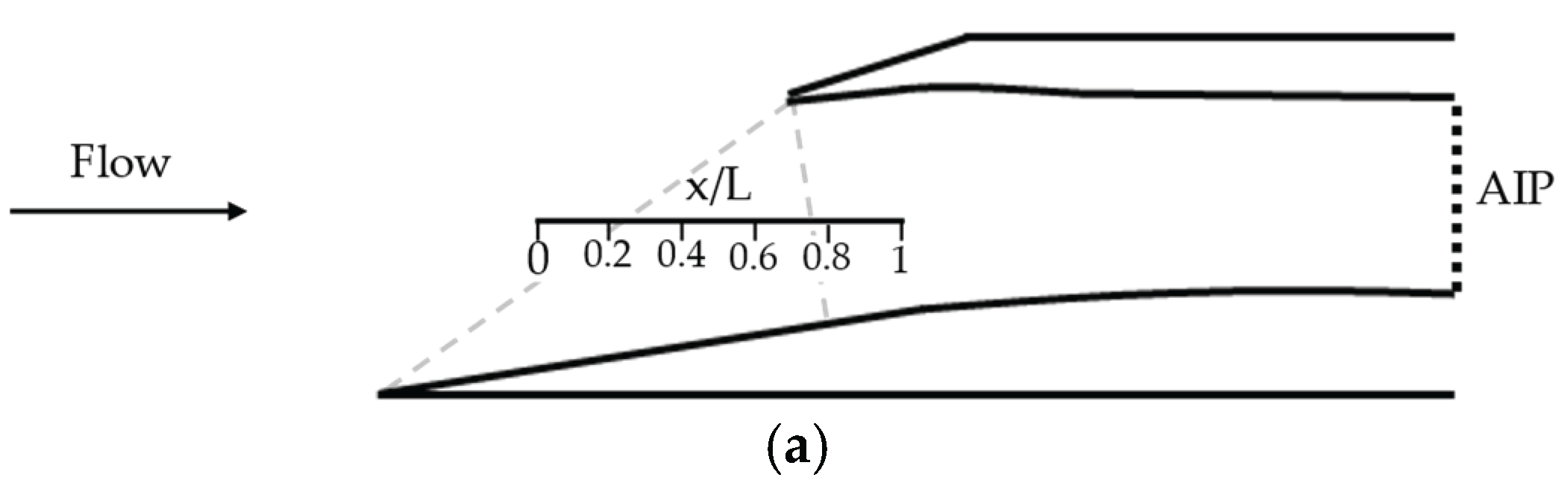
Figure 10.
Comparisons of streamwise Mach-number distributions for different flow ratios (λ) a) along a line on the compression surface; at different freestream Mach numbers: b) M∞ = 1.4, c) M∞ = 1.5, d) M∞ = 1.6, e) M∞ = 1.7, f) M∞ = 1.8, and g) M∞ = 1.9.
Figure 10.
Comparisons of streamwise Mach-number distributions for different flow ratios (λ) a) along a line on the compression surface; at different freestream Mach numbers: b) M∞ = 1.4, c) M∞ = 1.5, d) M∞ = 1.6, e) M∞ = 1.7, f) M∞ = 1.8, and g) M∞ = 1.9.
3.3. Mach Distribution Along Compression Surface
Figure 10 provides detailed flow-field evidence to explain the wall shear stress trends observed in
Figure 9.
Figure 10 illustrates the streamwise Mach number distributions along the compression surface for each M
∞ at several different
λ. The plots clearly visualize the upstream movement of the terminal shock system as
λ is reduced (i.e., as back pressure increases) toward the ‘buzz onset’ limit.
3.4. Boundary Layer Control Mechanism Requirement
The crucial insight is that the strength of this terminal shock (specifically, its upstream of the normal shock Mach number, M
n) is the decisive parameter. A well-established criterion in aerodynamics states that a shock with M
n =1.32 is typically strong enough to induce turbulent boundary layer separation [
2].
The data presented in
Figure 11 provides the definitive justification for the necessity of boundary layer control. The plot clearly shows the M
n of the terminal shock relative to the M
∞. At M
∞ = 1.4, and 1.5, the shock strength remains sub-critical M
n < 1.3. However, at M
∞ = 1.6, the shock strength M
n = 1.32 explicitly crosses the ‘Critical Mach’ threshold, which is the established criterion for shock-induced turbulent boundary layer separation.
At all higher Mach numbers from M∞ = 1.7 to 1.9, the Mn value continues to increase, guaranteeing the formation of extensive flow separation. Given that this unavoidable separation is the root cause of both performance loss (as identified in the τw analysis) and critical instability (buzz), it is concluded that a boundary layer bleed (WB) system is an essential design requirement for achieving stable and efficient operation of the inlet for all M∞ >1.6.
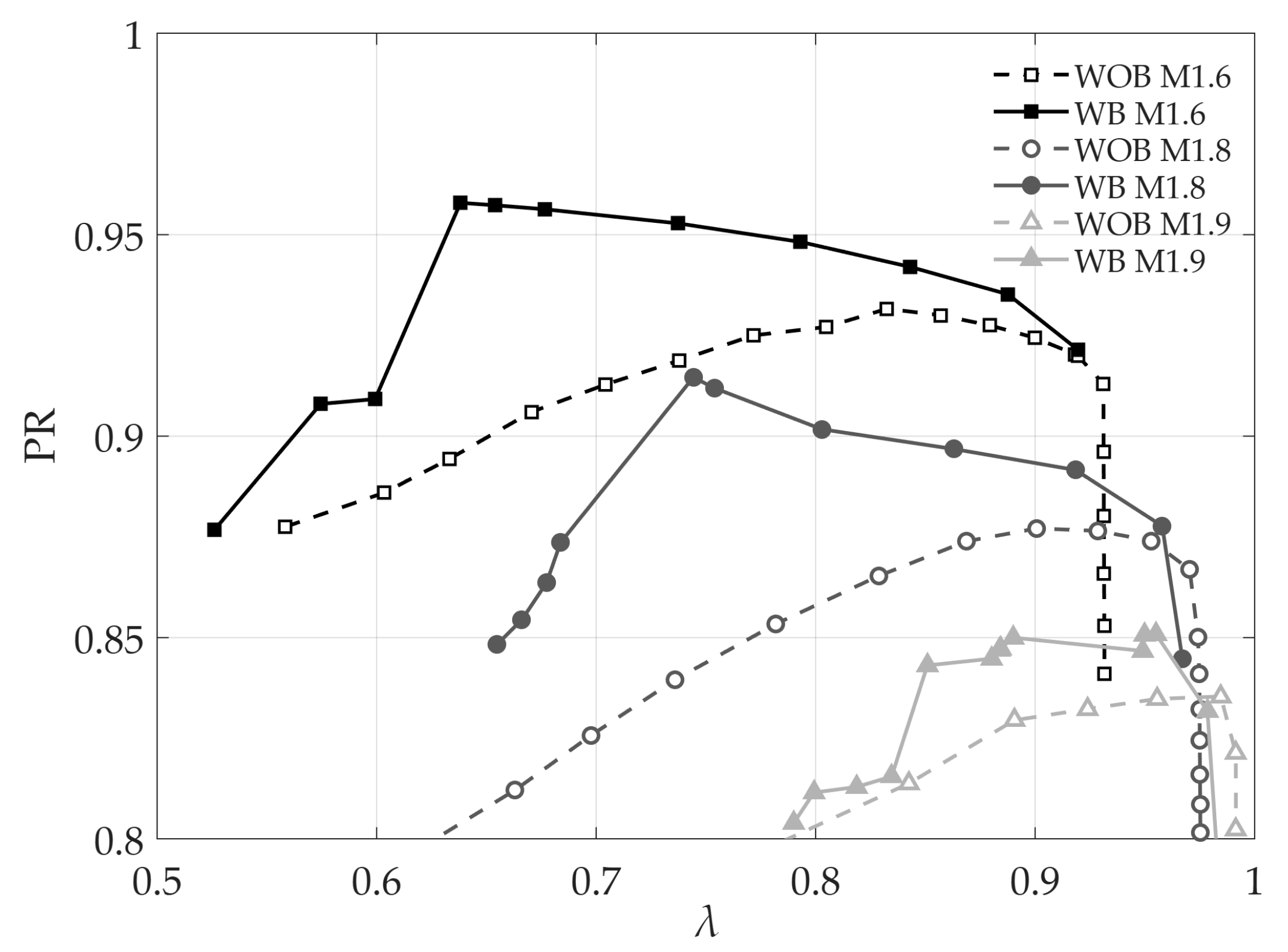
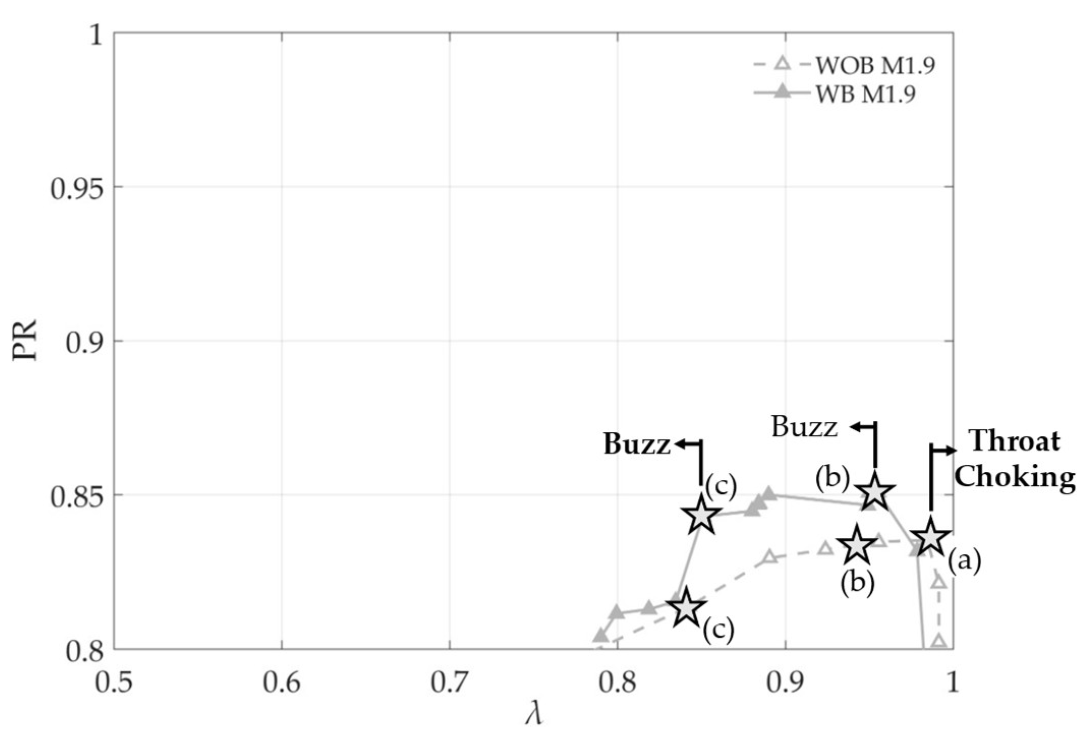
3.5. Bleed System Effect on Intake Stability
Figure 12 shows that implementing a boundary layer bleed system considerably improves the stability margin of the supersonic inlet, principally by delaying the onset of aerodynamic instabilities such as buzz. As seen in the
PR versus
λ characteristics, the bleed system enables the inlet to work stably down to lower
λ values when compared to the non-bleed arrangement. As a result, the bleed system effectively expands the stable operational envelope towards lower mass flow conditions, increasing the inlet’s tolerance to downstream disturbances or backpressure fluctuations before instability occurs, and thus improving the overall stability margin across the tested freestream Mach numbers.
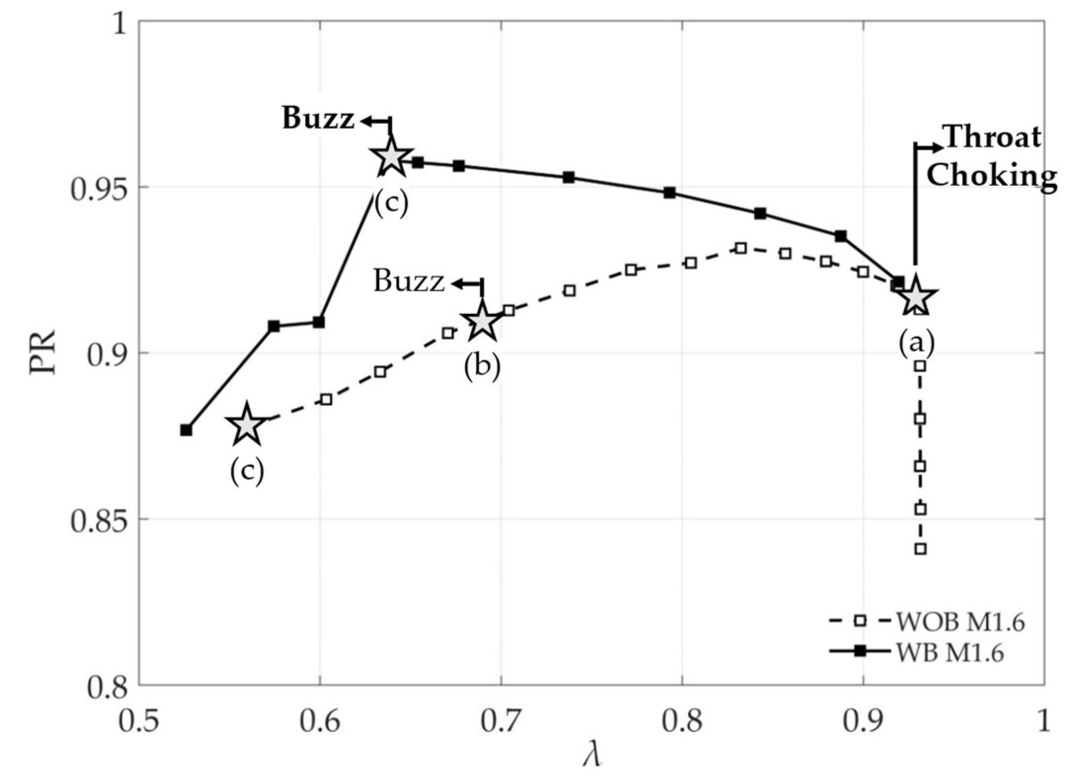
Figure 13 depicts the operational parameters of the supersonic inlet at Mach 1.6, comparing performance WB (solid line) and WOB (dashed line) by graphing
PR against the
λ. The curves distinguish three key operating regimes. The first is (a) supercritical operation, which terminates at the ‘Throat Choking’ limit. This point (a) represents the maximum mass flow rate capacity of the inlet; any further increase in
λ cannot pass additional mass flow as the throat is choked. As
λ is reduced, the inlet enters (b) critical operation, defined here as the onset of low-frequency buzz. This instability (b) is understood to begin when the shear layer, originating from the triple point of the shock interaction, starts to be ingested into the duct. Further reductions in
λ lead to (c) subcritical operation, which is initiated by the onset of high-frequency buzz (c). This final regime is characterized by significant boundary layer separation and is observed on the graph as a region of sudden, sharp drops in
PR. The activation of the bleed system results in significant benefits; it enhances the maximum possible
PR, raises
PR levels across the subcritical range, and crucially, improves inlet stability by delaying the onset of both buzz instabilities (points b and c) to much lower
λ values, thereby expanding the stable operating range.
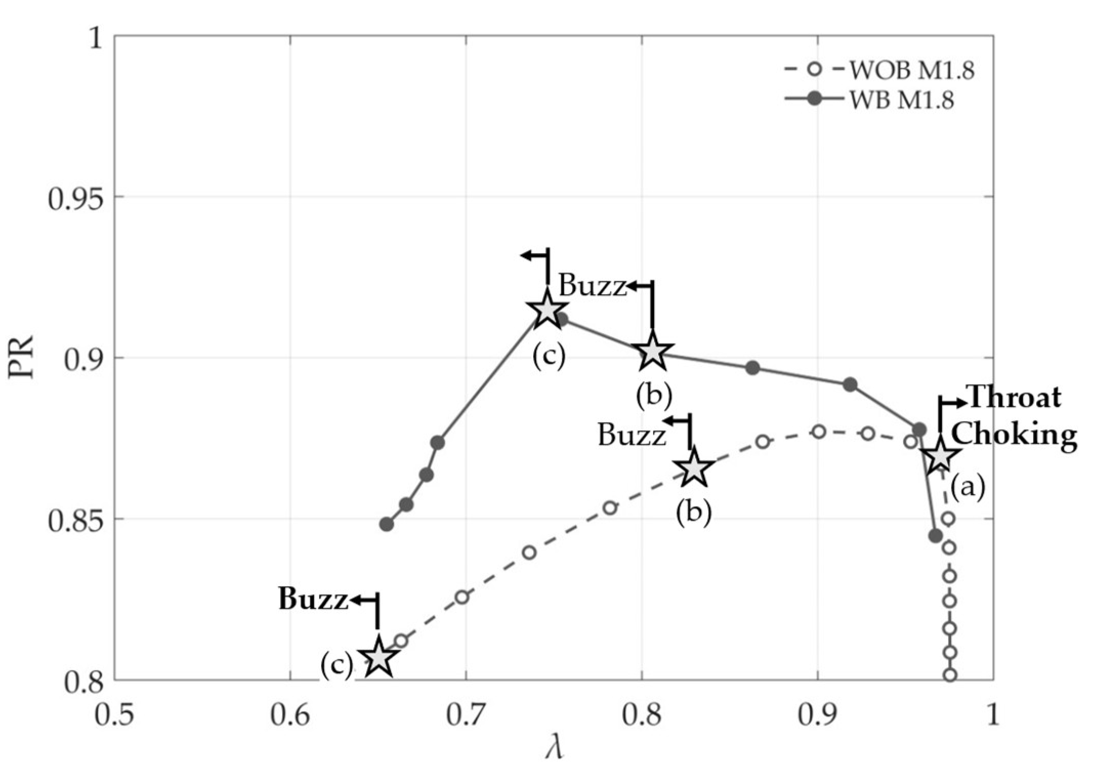
Figure 14 presents the performance characteristics of the inlet at M
∞ = 1.8, comparing the WB (solid line) and WOB (dashed line) configurations. The plot of
PR versus the
λ clearly shows that the WB case achieves a significantly higher peak
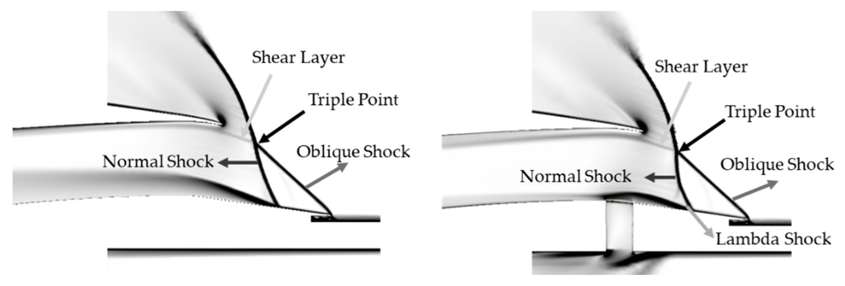
PR than the WOB case. Critical operating points are also marked, including the ‘Throat Choking’ limit (a) and the ‘Buzz’ instability onsets (b and c), illustrating the differences in stability.
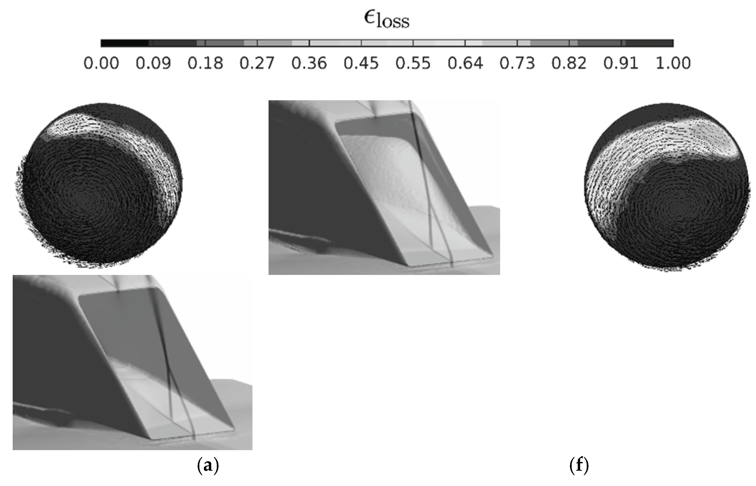
Figure 15 provides the physical explanation for this performance difference by visualizing the flow structure at two specific operating points near the “Buzz (b)” stability limit. The WOB condition
λ = 0.8287 shows a strong SBLI. A Normal Shock interacts with the wall’s boundary layer, creating a Triple Point and a large Shear Layer, which indicates flow separation. This separation is inefficient and contributes to the lower
PR and instability seen in the WOB curve. The WB condition
λ = 0.8057 demonstrates the effect of bleed. The bleed actively removes the low-energy boundary layer. This suction alters the SBLI, causing the shock to bifurcate (split) at its base, forming a characteristic Lambda Shock structure. This control of the boundary layer prevents large-scale separation, stabilizes the shock system, and is the direct cause of the superior
PR and stability documented for the WB configuration in
Figure 14.
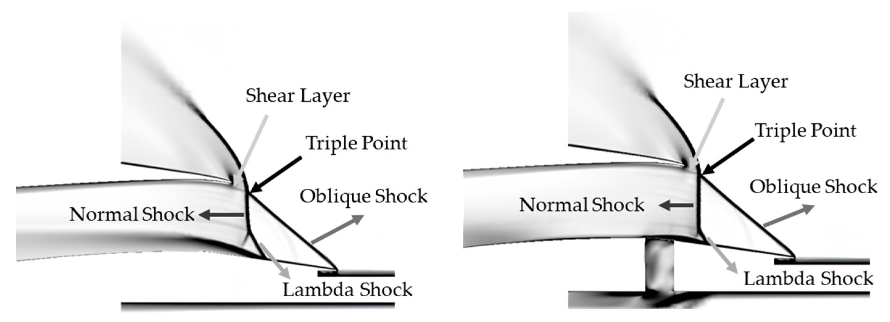
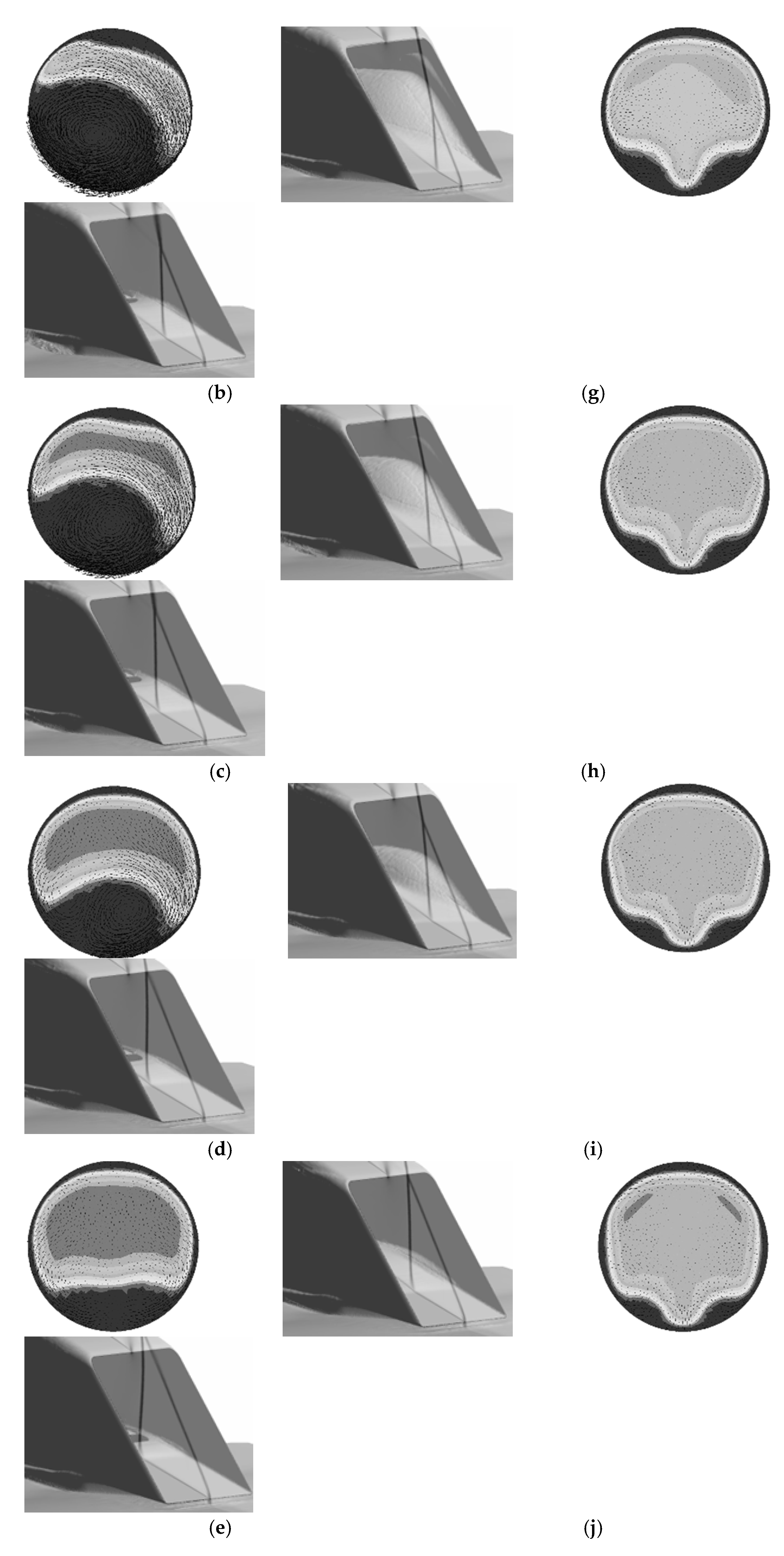
Figure 16 displays the performance characteristics for the inlet at M
∞ = 1.9, comparing the WB (solid line) and WOB (dashed line) configurations.
Figure 17 provides the physical explanation for the performance difference observed at Mach 1.9, visualizing the flow structure at specific operating points for both configurations. The WOB condition (left, at
λ = 0.942) visualizes the baseline SBLI. A primary Normal Shock interacts with the boundary layer, leading to the formation of a Triple Point, an Oblique Shock, and a subsequent Shear Layer. A small Lambda Shock structure is also visible at the foot, indicating the presence of flow separation. This separation is the source of the pressure losses and instability documented for the WOB case in
Figure 16. The WB condition (right, at
λ = 0.951) demonstrates the effect of bleed. The bleed, positioned directly under the interaction, actively removes the low-energy boundary layer. This suction modifies the SBLI, promoting a more stable and pronounced Lambda Shock structure at the foot. By controlling the boundary layer in this manner, the bleed system prevents large-scale separation, anchors the terminal shock, and is the direct cause of the enhanced
PR and stability documented for the WB configuration in
Figure 16.
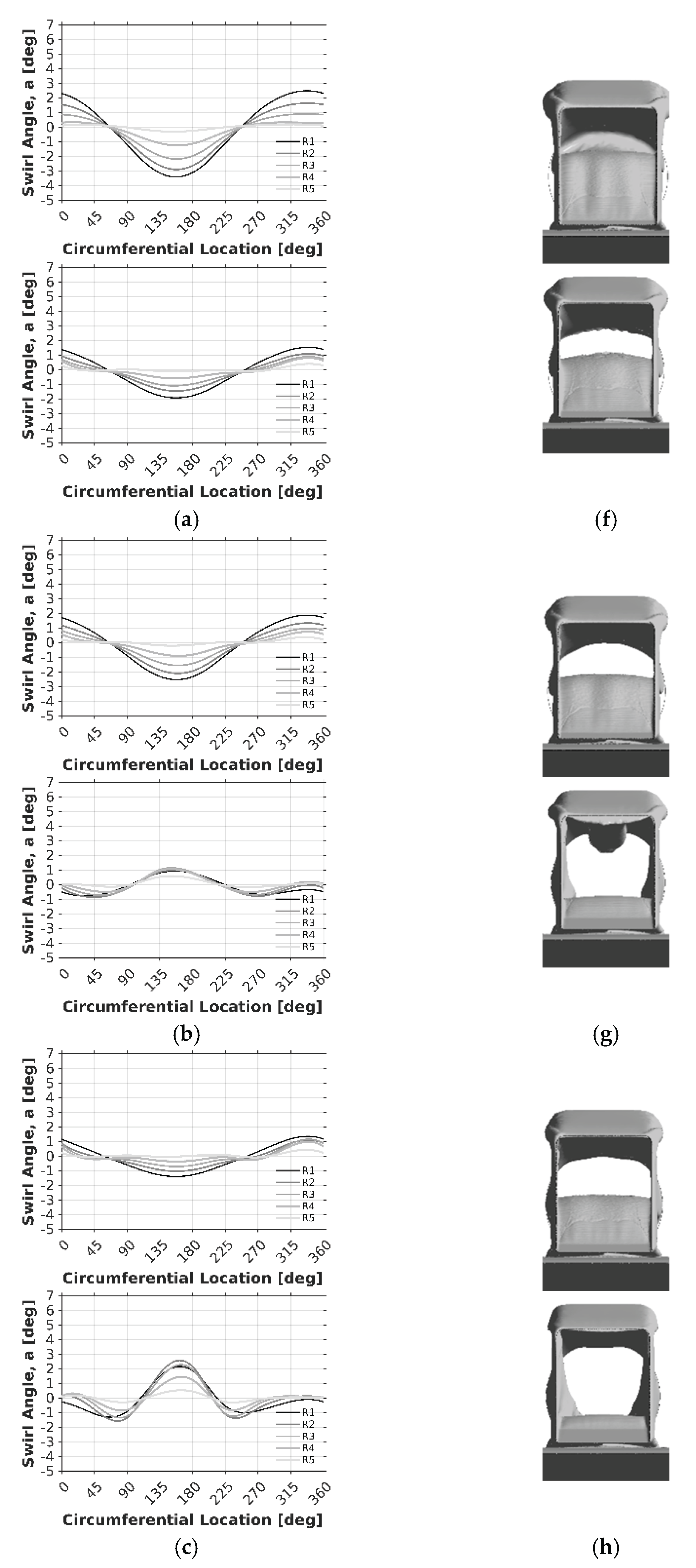
3.6. Circumferential Swirl Angle Distributions
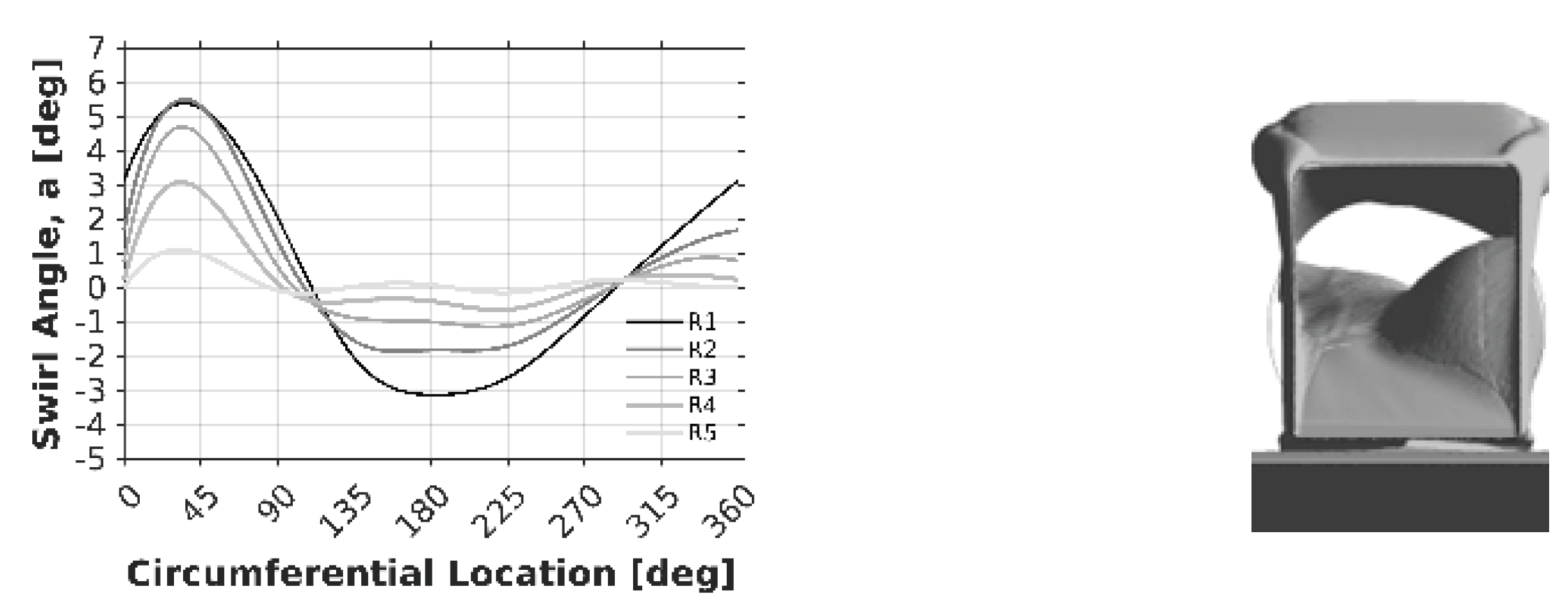
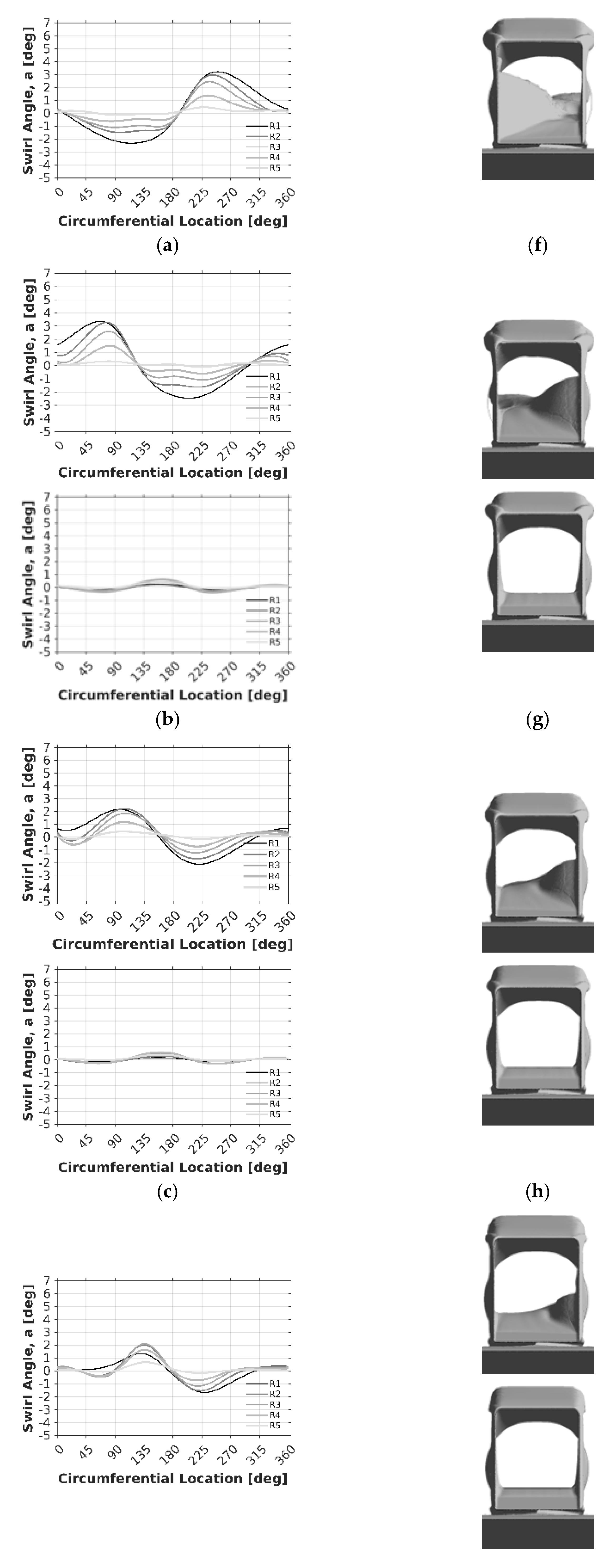
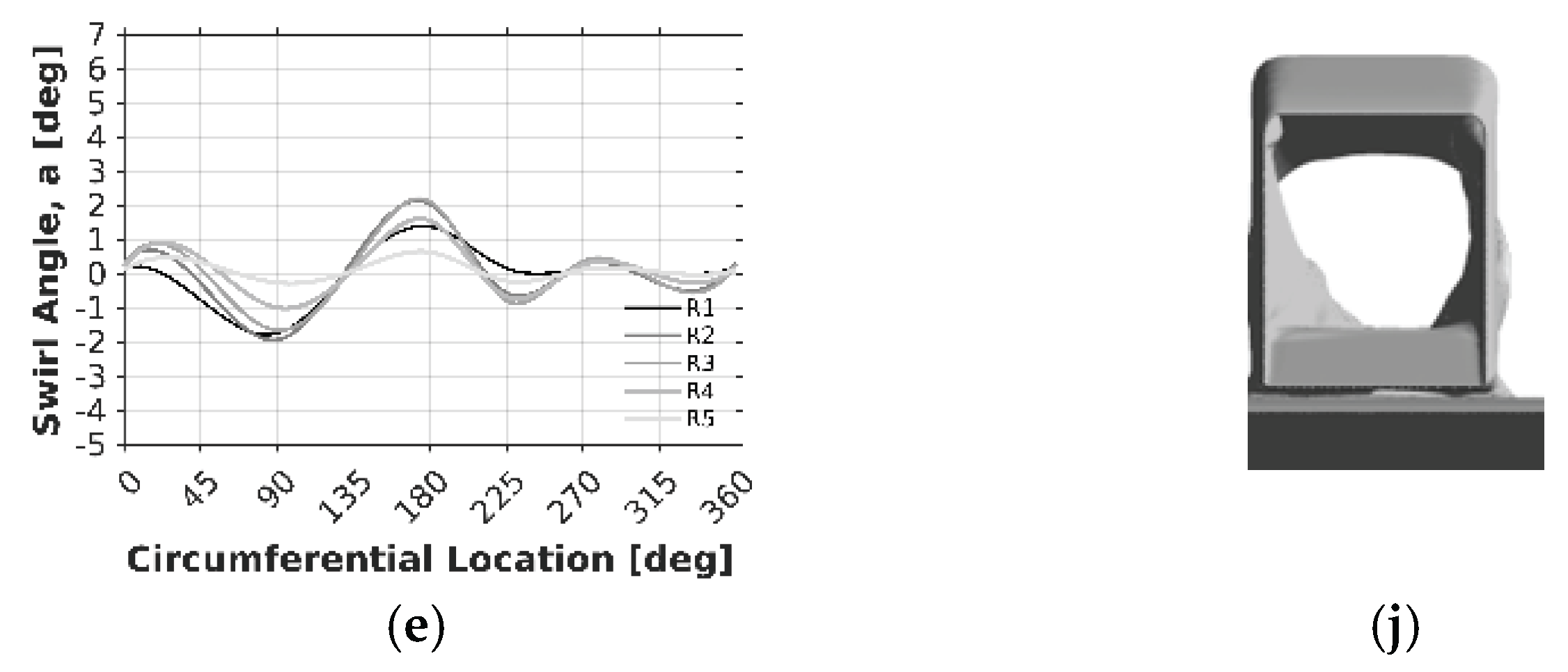
Figure 18 shows the swirl angle (
α) distribution at the AIP over five radial rings (R1 to R5) at M
∞ = 1.6. The results are presented for
λ values ranging from 0.57 to 0.84. Each subfigure depicts both the swirl angle variation and the
ϵloss iso-surface at the AIP plane. The left column shows the baseline (no bleed, WOB) case, whereas the right column shows the bleed-enabled cases.
In the absence of bleed, the swirl angle profiles show significant circumferential asymmetry and increased amplitude, especially at lower λ values. At λ = 0.57, the swirl angle ranges from ±6°, with the inner rings (R1-R3) showing the most significant variances. This phenomenon is strongly related to sidewall separation and the subsequent SBLI, which causes concentrated swirling motion at the separated region. Visual confirmation for these swirl patterns comes from the accompanying ϵloss iso-surfaces, which show a thick pressure loss structure skewed toward the separated side. As λ increases, the amplitude and asymmetry of the swirl angle profiles gradually diminish, indicating a return to flow symmetry as the boundary layer reattaches and the separation bubble weakens. Nonetheless, even at λ = 0.79, residual swirl asymmetry is discernible in both the angular plots and the ϵloss contours.
In contrast, bleed-enabled situations exhibit a significant reduction in SI and distortion across all λ values. At λ = 0.57, swirl profiles flatten dramatically, reducing peak values to ±2° and suppressing radial variance between rings. This homogeneity is further represented in the ϵloss contours, which have smooth and symmetric pressure loss distributions, with the high-loss zones significantly reduced. The bleed action appears to reduce SBLI-induced separation along the sidewall, resulting in a more symmetrical and stable inlet flow field. As λ increases, the swirl profiles remain flat and relatively uniform, while the ϵloss distributions show little further change, indicating that the incoming flow has entered a highly stable state.
Taken together, these findings show that applying bleed flow efficiently decreases swirl production by reducing separation-driven vorticity and restoring circumferential symmetry at the AIP. The ϵloss iso-surfaces provide a valuable qualitative correlate to swirl angle trends, supporting the fact that when bleed is activated, inlet symmetry and aerodynamic performance improve dramatically across the entire λ working range.
Figure 19 depicts iso-surfaces of the ϵ
loss and accompanying swirl vector fields at the AIP spanning five
λ values for both WOB (left) and WB (right) configurations. For the baseline (no bleed) cases, there is a clear evolution of the separation pattern and swirl asymmetry: at
λ = 0.57, a strong sidewall-originating vortex dominates the flow structure, producing high swirl angle magnitudes and elevated ϵ
loss values concentrated along the left side of the AIP. As λ increases, the intensity and footprint of this divided zone gradually decrease, although traces of the asymmetry continue until
λ = 0.79. In contrast, the bleed-enabled setup results in a significant reduction in both swirl strength and ϵ
loss intensity, beginning with the lowest
λ case. Circumferential symmetry has been restored in the flow vectors, and high-loss zones are either greatly limited or missing.
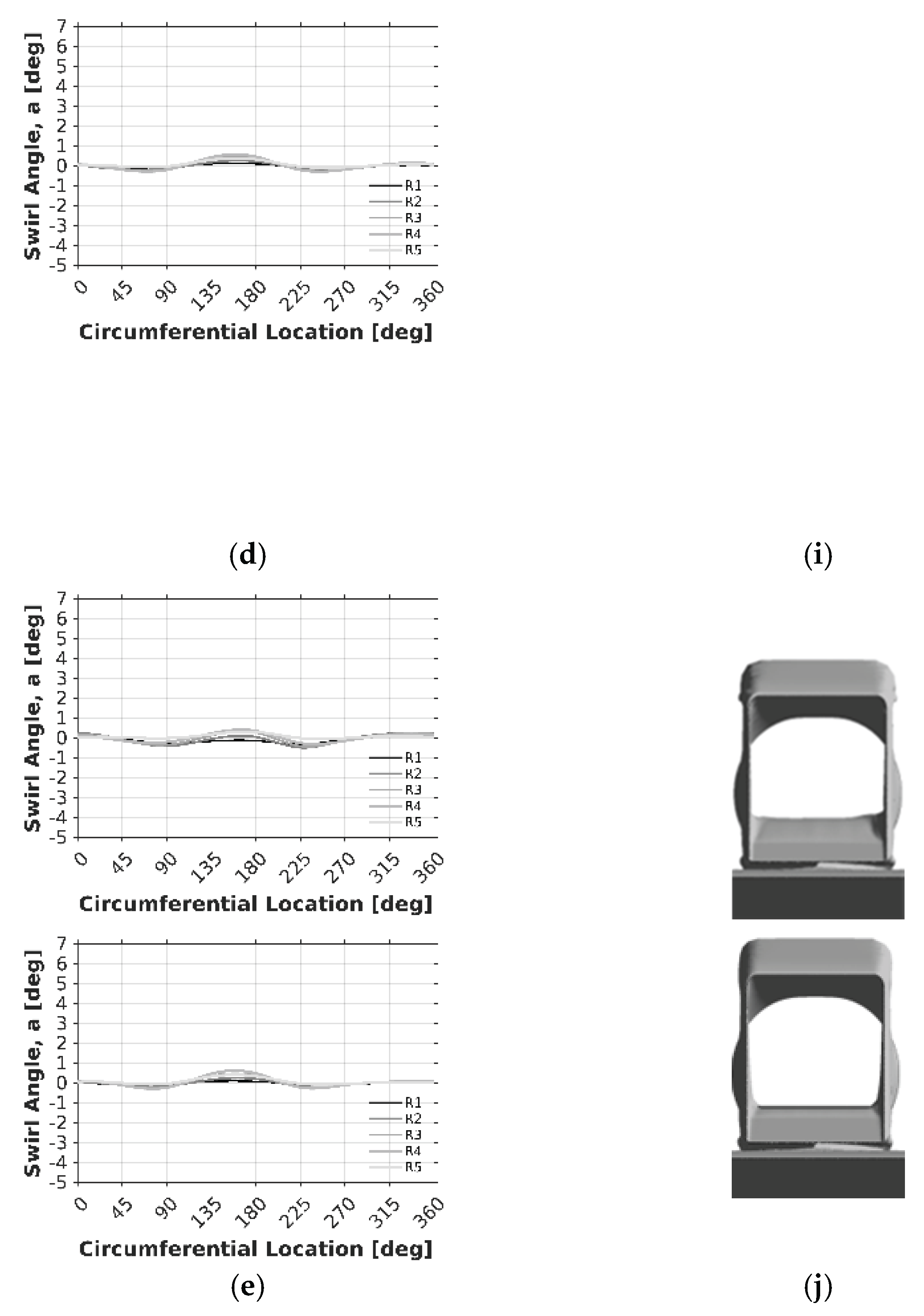
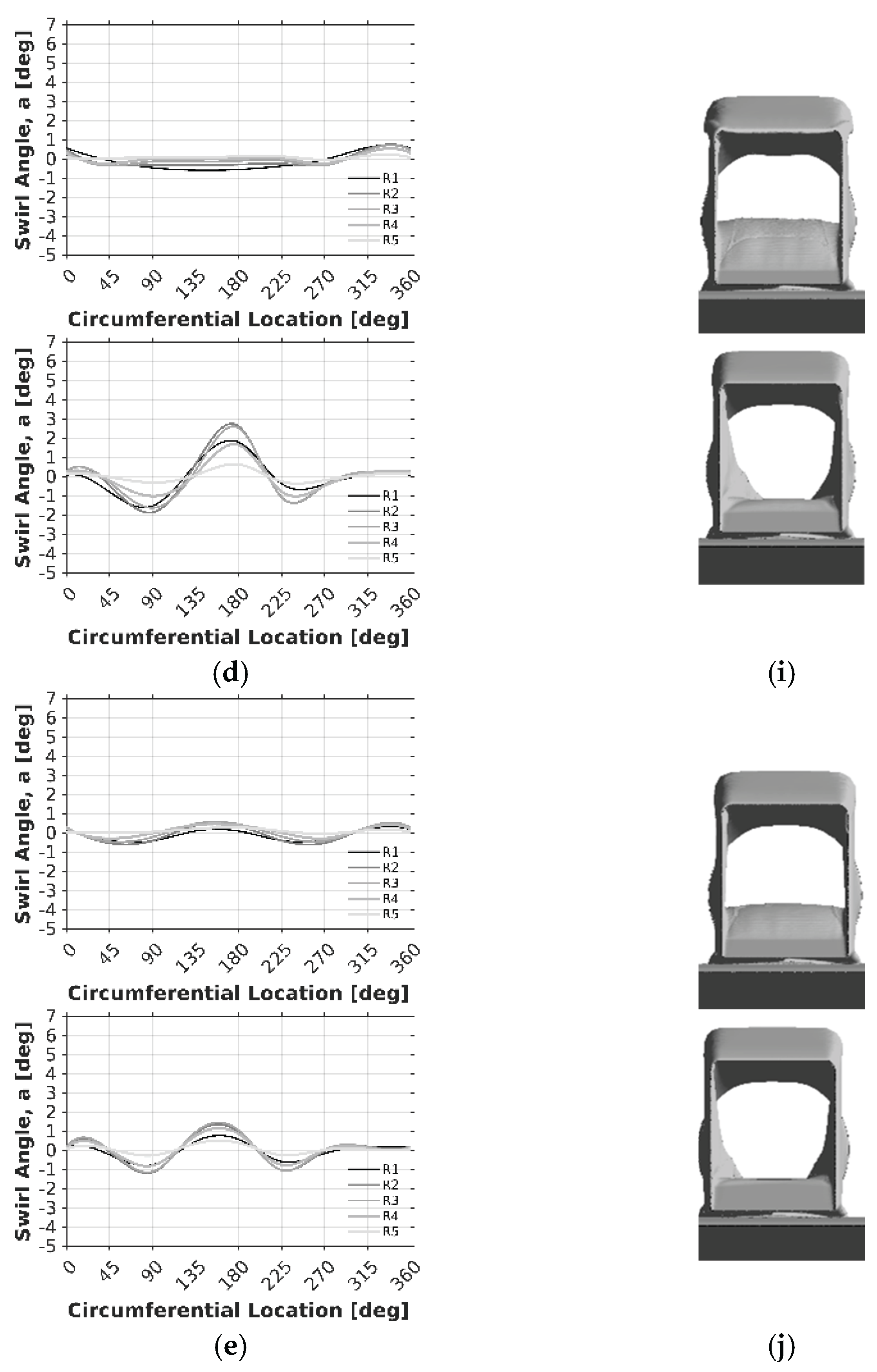
Figure 20 shows a detailed investigation of the swirl angle (α) distribution over the AIP for a supersonic intake with M
∞ = 1.8. The WOB data (a-e) show significant swirl distortion, defined by organized patterns with distinct positive and negative swirl zones, notably at lower λ values (a, b), reaching magnitudes of up to approximately ±4 degrees. These patterns, which indicate organized vortical structures, correspond to the asymmetric flow features shown in the corresponding schematic views and gradually decrease in intensity as λ increases. However, engaging the bleed system (WB, plots f-j) results in a significant improvement in flow quality. Swirl angle magnitudes are reduced to below ±2 degrees, resulting in more consistent circumferential profiles across all radial sites. This enhanced homogeneity is reflected in the more symmetric patterns seen in the accompanying AIP diagrams. While certain low-amplitude wavy variations persist in the WB cases at intermediate λ (h, i), overall swirl distortion is much reduced, proving the bleed system’s ability to manage flow angularity at Mach 1.8.
In
Figure 21, the swirl angle (
α) distribution at the AIP for a supersonic intake operating at M
∞ = 1.9 is compared between the baseline WOB, left column, a-e and the WB, right column, f-j across
λ from 0.68 to 0.95. At high Mach numbers, swirl angle magnitudes in the WOB configuration (a-e) remain considerable, but generally smaller than at M=1.6, with peaks reaching roughly ±3-4 degrees. The patterns show clear structure, with dominant negative swirl near the 180° circumferential location, especially at lower
λ (a, b, c), indicating organized vortical flow caused by flow separation phenomena within the inlet duct, as supported by the asymmetric AIP flow patterns in the accompanying schematics. As
λ grows (from a to e), the swirl magnitude decreases. The WB arrangement (f-j) reduces swirl angles to ±2 degrees, leading to more uniform flow patterns over AIP rings and circumference. Although the bleed cases have much flatter profiles overall, some residual low-amplitude swirl structure can still be seen (e.g., plot i,
λ = 0.87), but the large-scale distortion seen in the WOB cases has been effectively suppressed, indicating successful mitigation of the primary swirl-inducing mechanisms.
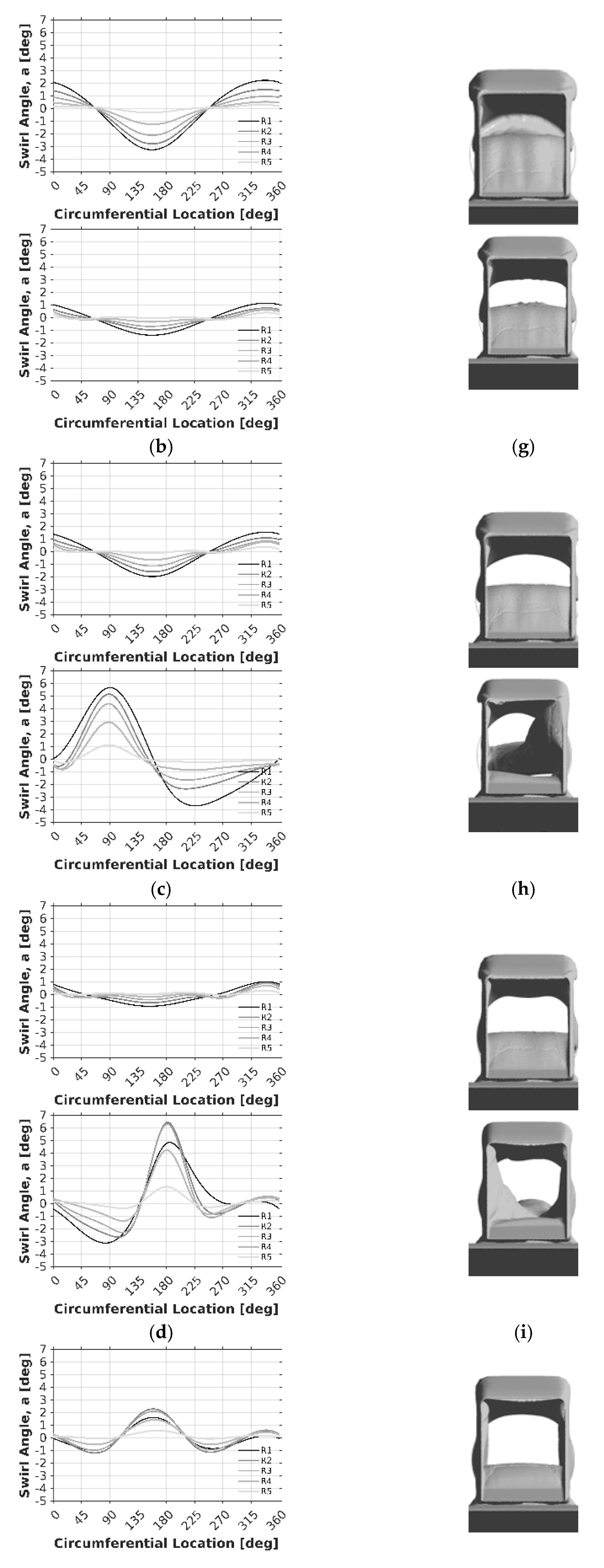
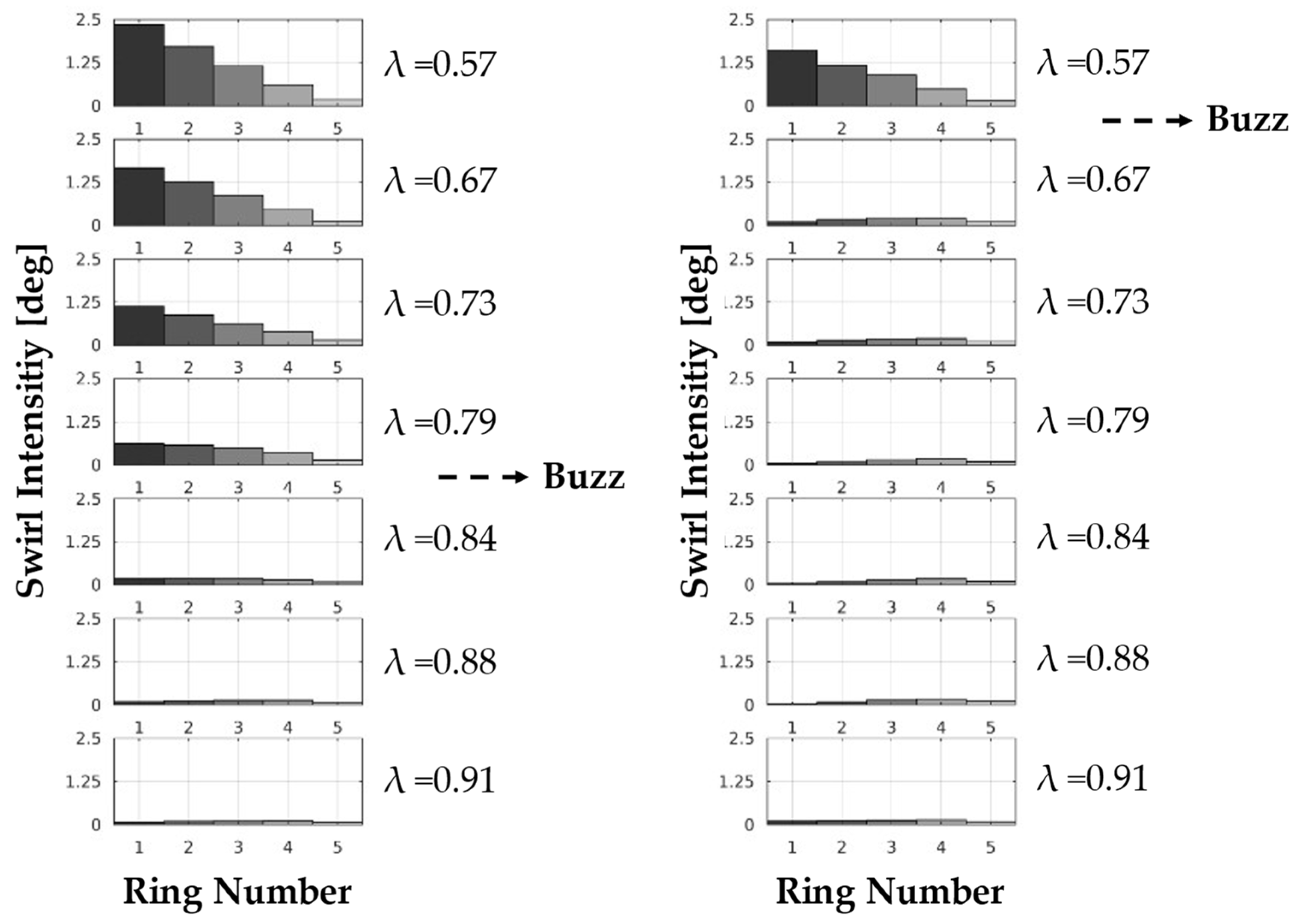
3.7. Circumferential Swirl Intensity Distributions
Figure 22 shows a quantitative assessment of SI, resolved radially, for an intake operating at M
∞ = 1.6. In the WOB scenario, significant SI is found at lower λ values (0.57 to 0.91), mainly focused in the inner rings (R1, R2), with peak values reaching around 2.5 degrees in Ring 1 at λ = 0.57. The intensity diminishes radially outward towards Ring 5. SI decreases sharply across all rings as λ increases beyond the specified buzz onset threshold about λ = 0.79, with values becoming negligible at λ = 0.84 and higher. In contrast, activating the bleed system has a significant influence on reducing SI. Across the entire λ range, the SI values are significantly lower than in the WOB scenario, typically remaining far below 1 degree and frequently close to zero for all rings. The consistently low SI levels in the WB configuration, even at low λ before buzz onset (lower than WOB’s), demonstrate the bleed system’s effectiveness in mitigating the development of strong vortical structures responsible for swirl across all measured radial locations and operating conditions at M
∞ = 1.6.
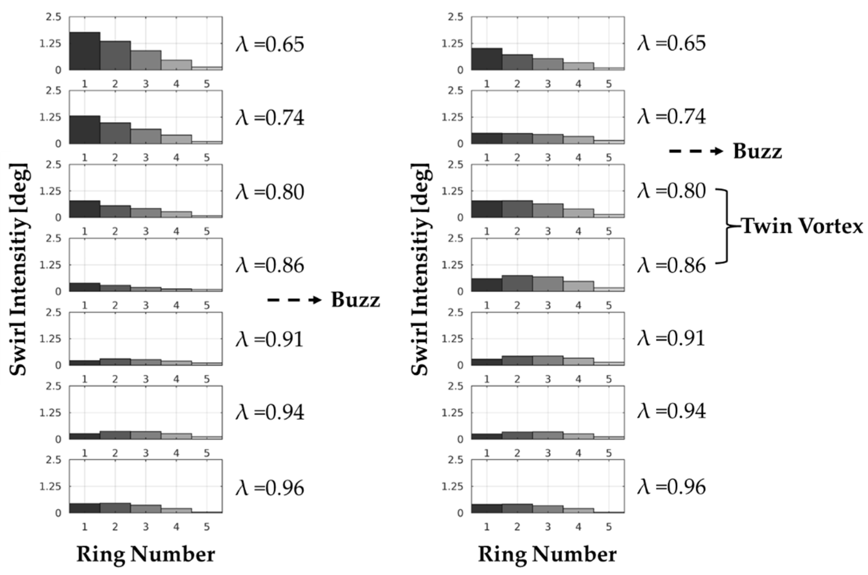
Figure 23 depicts the radially resolved
SI features at 1.8, over a
λ range of 0.65 to 0.96. In the WOB arrangement, the
SI is moderately high at lower
λ values (0.65 to 0.86), peaking at 1.5 degrees in the inner rings (R1, R2) and decreasing radially outwards. Similar to the Mach 1.6 scenario, as the
λ increases beyond the buzz beginning point (shown near
λ = 0.86), there is a noticeable decline in intensity throughout all rings. In contrast, the bleed system produces a significant reduction in
SI throughout all rings and
λ, with values typically remaining below 1 degree. The radial distribution is likewise much more uniform than in the WOB example. Surprisingly, despite the overall low intensity levels, the presence of a “Twin Vortex” structure matching to
λ = 0.80 and 0.86 in the WB data. This shows that, while the bleed system effectively reduces the overall amplitude of the swirl, residual structured flow structures, maybe corresponding with modest wavy patterns in swirl angle distributions, may exist under certain operating conditions even when the bleed system is functioning.
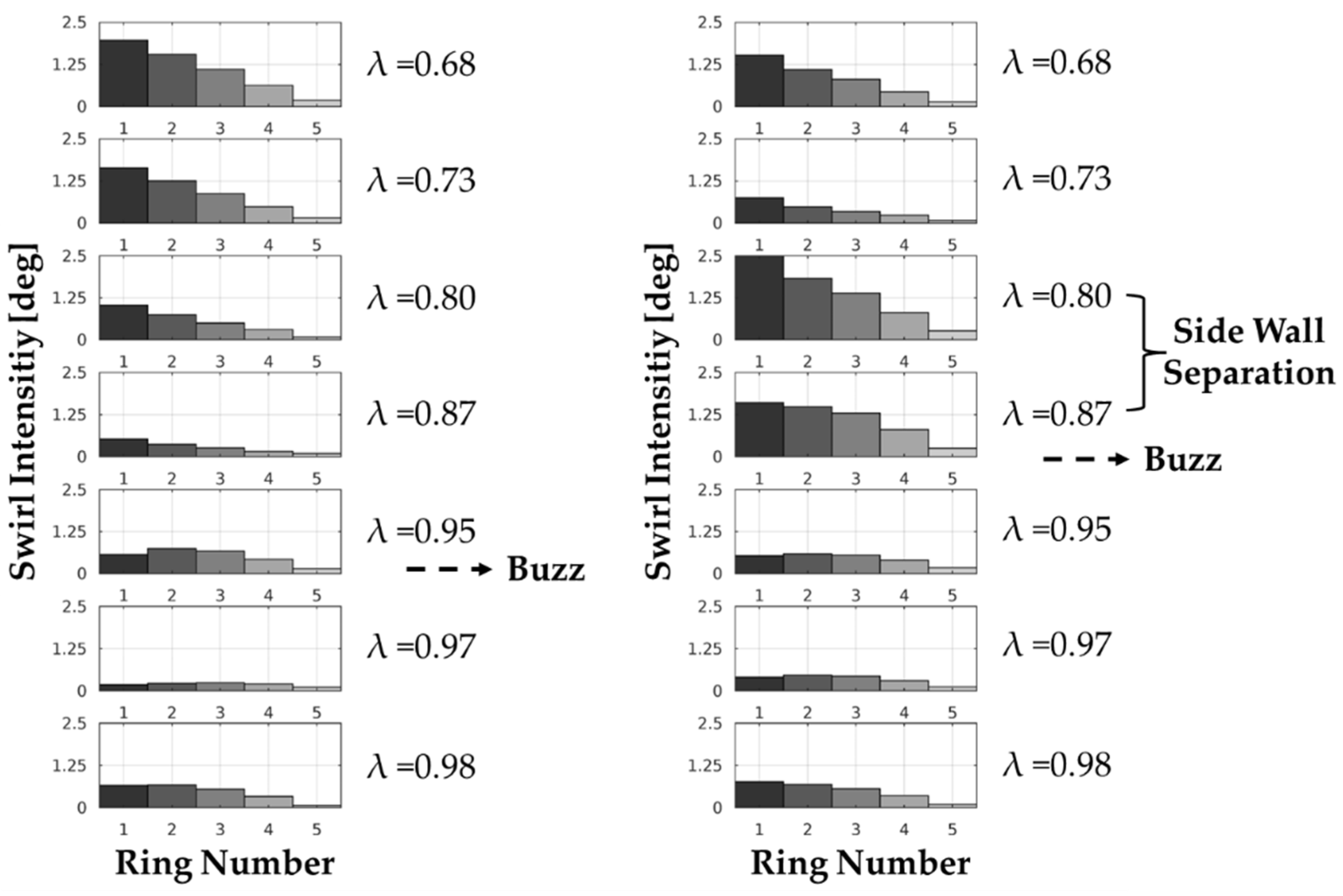
Figure 24 depicts the radially resolved
SI features at the AIP at M
∞ = 1.9, throughout a
λ range of 0.68 to 0.98. In the WOB arrangement, the
SI is quite high at lower
λ values (0.68 to 0.95), peaking at 1.5 degrees in the inner rings (R1, R2) and decreasing radially outwards. Similar to the Mach 1.6 case, a significant decline in intensity happens throughout all rings when the
λ rises over the buzz initiation point. The radial distribution is likewise much more uniform than in the WOB example. Surprisingly, despite the overall low intensity levels, there is a “side wall separation” structure in the WB data with
λ values of 0.80 and 0.87. This shows that, while the bleed system effectively reduces the overall amplitude of the swirl, residual structured flow structures, maybe corresponding with modest wavy patterns in swirl angle distributions, may exist under certain operating conditions even when the bleed system is functioning.
3.8. Map-Level Trends and Physical Mechanism
Across M∞ = {1.6, 1.8, 1.9}, WOB cases exhibit SBLI-driven separation that elevates swirl at low λ and weakens toward the buzz onset, whereas WB consistently yields lower SI at matched λ. At M∞ = 1.6, strong corner vortices dominate the swirl signature near λ of 0.57; as λ increases, corner-vortex strength decays and SI drops, becoming negligible beyond λ = 0.84. At M∞ = 1.8, the separation peak is observed near λ = 0.65, producing the highest WOB SI; under WB at the same λ, separation persists but SI remains markedly lower. Between λ = 0.80 - 0.86, WB may show “twin corner-vortex” traces that wane with increasing λ. At M∞ = 1.9, trends mirror the M∞ = 1.8 case; under WB, sidewall-separation signatures can appear around λ = 0.80 yet SI stays unusually low, indicating that bleed alters the separation footprint and de-organizes swirl sectors.
3.9. Bleed-Onset Threshold and Operability Implications
Once the pre-shock normal Mach number exceeds Mn = 1.32, separation is triggered without bleed, setting the practical bleed-onset threshold for M∞ > 1.6. With WB, near-wall low-momentum fluid is overboarded and the terminal shock footprint is stabilized into a Λ-type pattern, PR increases and SI decreases across the operating map. Consequently, the last stable point shifts to lower λ at fixed M∞ extending the stable operating range while keeping SIRA / SISA within guideline levels.
3.10. Modeling Considerations and Limitations
The WB configuration is implemented via a porous-jump surrogate fitted to hole-resolved 3-D RANS data. The viscous (F1) and inertial (F2) resistances are expressed through a quadratic ∆p-V relation at the exit-plane superficial velocity, parameterized by porosity, L/D, and hole diameter. The flow solution is obtained with the steady-state RANS (realizable k−ε, EWT). High-frequency buzz dynamics, plenum–structure coupling, and unsteady bleed–shock interactions are not resolved.
Figure 1.
Geometry of the single ramp external supersonic compression intake model [
17].
Figure 1.
Geometry of the single ramp external supersonic compression intake model [
17].
Figure 2.
(a) Rectangular computational domain around the supersonic inlet. (b) Detailed views of the unstructured computational grid with refinement near the inlet surfaces.
Figure 2.
(a) Rectangular computational domain around the supersonic inlet. (b) Detailed views of the unstructured computational grid with refinement near the inlet surfaces.
Figure 3.
Grid-parameter map for the grid-independence study.
Figure 3.
Grid-parameter map for the grid-independence study.
Figure 4.
Comparisons of the results for four different grid resolutions (1.5 M, 4 M, 39 M, and 82 M cells) with the experimental (tunnel) data: (a) pressure distribution along the compression surface (P01-P07); (b) pressure distribution along the splitter plate (P08-P12).
Figure 4.
Comparisons of the results for four different grid resolutions (1.5 M, 4 M, 39 M, and 82 M cells) with the experimental (tunnel) data: (a) pressure distribution along the compression surface (P01-P07); (b) pressure distribution along the splitter plate (P08-P12).
Figure 5.
Grid-independence study: Pressure recovery change with grid size at the operating condition at M∞ = 1.8 and λ = 0.97.
Figure 5.
Grid-independence study: Pressure recovery change with grid size at the operating condition at M∞ = 1.8 and λ = 0.97.
Figure 6.
The 8×5 rake model for total pressure measurement at the AIP.
Figure 6.
The 8×5 rake model for total pressure measurement at the AIP.
Figure 7.
Flowchart for swirl angle classification and integration [
22].
Figure 7.
Flowchart for swirl angle classification and integration [
22].
Figure 8.
Pressure recovery versus flow ratio for different Mach numbers, M∞ = 1.4-1.9.
Figure 8.
Pressure recovery versus flow ratio for different Mach numbers, M∞ = 1.4-1.9.
Figure 11.
Wall shear stress versus freestream Mach number. Each data point is with the corresponding Mach number upstream of the normal shock. The vertical dotted line indicates the ‘Critical Mach’ at Mn = 1.32 (corresponding to M∞ = 1.6).
Figure 11.
Wall shear stress versus freestream Mach number. Each data point is with the corresponding Mach number upstream of the normal shock. The vertical dotted line indicates the ‘Critical Mach’ at Mn = 1.32 (corresponding to M∞ = 1.6).
Figure 12.
Pressure recovery versus flow ratio, with bleed (WB, solid line) and without bleed (WOB, dashed line), for three different Mach numbers M∞ = 1.6, 1.8, and 1.9.
Figure 12.
Pressure recovery versus flow ratio, with bleed (WB, solid line) and without bleed (WOB, dashed line), for three different Mach numbers M∞ = 1.6, 1.8, and 1.9.
Figure 13.
Pressure recovery versus flow ratio for the Mach 1.6 inlet (M∞ = 1.6) with bleed (WB, solid line with squares) and without bleed (WOB, dashed line with squares).
Figure 13.
Pressure recovery versus flow ratio for the Mach 1.6 inlet (M∞ = 1.6) with bleed (WB, solid line with squares) and without bleed (WOB, dashed line with squares).
Figure 14.
Pressure recovery versus flow ratio for the Mach 1.8 inlet (M∞ = 1.8) with bleed (WB, solid line with squares) and without bleed (WOB, dashed line with squares).
Figure 14.
Pressure recovery versus flow ratio for the Mach 1.8 inlet (M∞ = 1.8) with bleed (WB, solid line with squares) and without bleed (WOB, dashed line with squares).
Figure 15.
Comparison of inlet shock structures and shear layer visualization at M∞ = 1.8 for WOB condition at λ = 0.8287 (left) and WB condition at λ = 0.8057 (right).
Figure 15.
Comparison of inlet shock structures and shear layer visualization at M∞ = 1.8 for WOB condition at λ = 0.8287 (left) and WB condition at λ = 0.8057 (right).
Figure 16.
Pressure recovery versus flow ratio for the Mach 1.8 inlet (M∞ = 1.8) with bleed (WB, solid line with squares) and without bleed (WOB, dashed line with squares).
Figure 16.
Pressure recovery versus flow ratio for the Mach 1.8 inlet (M∞ = 1.8) with bleed (WB, solid line with squares) and without bleed (WOB, dashed line with squares).
Figure 17.
Comparison of inlet shock structures and shear layer visualization at Mach 1.9 for WOB condition at λ = 0.942 (left) and WB condition at λ = 0.951.
Figure 17.
Comparison of inlet shock structures and shear layer visualization at Mach 1.9 for WOB condition at λ = 0.942 (left) and WB condition at λ = 0.951.
Figure 18.
Swirl angle distribution at the AIP for the supersonic intake at the freestream Mach 1.6, showing five rings (R1 to R5) across λ = 0.57 (a, f), 0.67 (b, g), 0.73 (c, h), 0.79 (d, i), and 0.84 (e, j), for WOB (left) and WB (right). The x-axis represents circumferential location (0° to 360°), and the y-axis shows swirl angle (degrees).
Figure 19.
Loss factor (ϵloss) contours and iso-surfaces at the AIP for M∞ = 1.6, without bleed (WOB) (a-e) and with bleed (WB) (f-j) configurations, at the same λ values of 0.57 (a, f), 0.67 (b, g), 0.73 (c, h), 0.79 (d, i), and 0.84 (e, j).
Figure 19.
Loss factor (ϵloss) contours and iso-surfaces at the AIP for M∞ = 1.6, without bleed (WOB) (a-e) and with bleed (WB) (f-j) configurations, at the same λ values of 0.57 (a, f), 0.67 (b, g), 0.73 (c, h), 0.79 (d, i), and 0.84 (e, j).
Figure 20.
Swirl angle distribution at the AIP for the supersonic intake at the freestream Mach 1.8, showing five rings (R1 to R5) across λ = 0.65 (a, f), 0.74 (b, g), 0.80 (c, h), 0.86 (d, i), and 0.91 (e, j), for WOB (left) and WB (right). The x-axis represents circumferential location (0° to 360°), and the y-axis shows swirl angle (degrees).
Figure 21.
Swirl angle distribution at the AIP for a supersonic intake at the freestream Mach 1.9, showing five rings (R1 to R5) across λ = 0.68 (a, f), 0.73 (b, g), 0.80 (c, h), 0.87 (d, i), and 0.95 (e, j), for WOB (left) and WB (right). The x-axis represents circumferential location (0° to 360°), and the y-axis shows swirl angle (degrees).
Figure 22.
Comparison of SI [deg] distribution across AIP rings (R1-R5) at at M∞ = 1.6 for WOB (left) and WB (right) configurations at λ from 0.57 to 0.91.
Figure 22.
Comparison of SI [deg] distribution across AIP rings (R1-R5) at at M∞ = 1.6 for WOB (left) and WB (right) configurations at λ from 0.57 to 0.91.
Figure 23.
Comparison of SI [deg] distribution across AIP rings (R1-R5) at M∞ = 1.8 for WOB (left) and WB (right) configurations at λ from 0.65 to 0.96.
Figure 23.
Comparison of SI [deg] distribution across AIP rings (R1-R5) at M∞ = 1.8 for WOB (left) and WB (right) configurations at λ from 0.65 to 0.96.
Figure 24.
Comparison of SI [deg] distribution across AIP rings (R1-R5) at M∞ = 1.9 for WOB (left) and WB (right) configurations at λ from 0.68 to 0.98.
Figure 24.
Comparison of SI [deg] distribution across AIP rings (R1-R5) at M∞ = 1.9 for WOB (left) and WB (right) configurations at λ from 0.68 to 0.98.
Table 1.
Test matrix for the inlet operating-map study.
Table 1.
Test matrix for the inlet operating-map study.
| Configuration |
M∞
|
Operating Sweep of Flow Ratio (λ) |
| Without Bleed (WOB) |
1.6, 1.8, 1.9 |
Supercritical → critical → subcritical
0.99 → 0.80 → 0.25 |
| With Bleed (WB) |