
Submitted:
12 November 2025
Posted:
13 November 2025
You are already at the latest version
Abstract
High-speed low-pressure turbines in geared turbofans operate at transonic exit Mach numbers and low Reynolds numbers. Engine-relevant data remain scarce. The SPLEEN C1 linear cascade is investigated at Mout=0.70--0.95 and Reout=65,000--120,000 under steady inlet flow. Experiments are combined with 2D RANS and MISES, including transition modelling and inlet-turbulence decay calibrated to measurements. Results are consistent with conventional LPT behaviour: losses decrease with increasing Mach and Reynolds numbers, except when shocks interact with the blade boundary layer (M≈0.95). Profile loss drops by 23% from M=0.70 to 0.95 at Re=70,000, and by 19% at M=0.80 when open separation is suppressed. Secondary loss decreases by up to 25% at Re=70,000 and shows weak sensitivity to Reynolds number. A coupled loss model predicts profile loss with RMSE=4.7%. Secondary-loss modelling reproduces global trends: separating endwall dissipation from mixing keeps errors within ±10% for most cases, but accuracy degrades near the shock–boundary layer interaction case and at the highest Reynolds number. Mixing dominates endwall loss (∼75%), with the passage vortex contributing ∼50% (±10%) of the mixing component. This article is a revised and expanded version of “An Experimental Test Case for Transonic Low-Pressure Turbines—Part 2: Cascade Aerodynamics at On- and Off-Design Reynolds and Mach Numbers” presented at ASME Turbo Expo 2022, Rotterdam, June 13–17, 2022. All data and documentation are openly available at https://doi.org/10.5281/zenodo.7264761.
Keywords:
high-speed low-pressure turbine
; linear cascade
; transonic
; laminar separation bubble
; secondary flows
; profile loss
; geared turbofan
; open-access dataset
1. Introduction
Ultra-high-bypass-ratio geared turbofans (GTFs) reduce and noise. For bypass ratios they enable lower specific fuel consumption, fewer low-pressure turbine stages, and reduced engine mass [13] – the low-pressure turbine (LPT) can account for one-third of the engine mass [14].
Torre et al. [15] investigated a high-speed LPT in a transonic rotating rig and documented key differences from conventional LPT operation. In geared architectures, the higher shaft speed drives the LPT blading sections to transonic exit Mach numbers () and low Reynolds numbers at cruise [16]. This combined transonic/low-Reynolds number regime is a principal challenge for GTF LPT design [17,18].
In conventional LPTs, profile losses typically exceed secondary losses because of their high aspect ratio [14]. Under engine-representative conditions, they can be comparable [19].
Vera et al. [20] showed that profile loss is nearly independent of Mach up to and rises beyond at . Vázquez et al. [21] observed increasing loss with Mach and decreasing loss with Reynolds number in an annular cascade. Both works attributed the Mach effect to higher dynamic pressure and altered suction side loading [20,21].
Perdichizzi [22] reported that higher outlet Mach confines secondary structures toward the endwall, reducing under/overturning and net loss. Mach and Reynolds effects were not decoupled for LPT conditions. Vázquez et al. [21] found endwall losses decrease with off-design Mach at fixed Reynolds number. Vázquez and Torre [23] confirmed the Mach effect at fixed incidence and linked it to off-design loading changes.
Hodson and Dominy [24] reported increasing secondary loss with Reynolds number near . Duden and Fottner [25] found secondary loss decreasing as both Mach and Reynolds increased for other LPT blades.
Despite this literature, few studies target the combined high Mach number, very-low-Reynolds number regime () that can exist in high-speed LPT blading. To our knowledge, no open database provides on- and off-design measurements for a high-speed LPT linear cascade.
This study extends the open SPLEEN C1 test case. Operating points spanned and under steady inlet flow. Experiments were combined with 2D Reynolds-averaged Navier–Stokes (RANS) computations and MISES with transition modelling. Inlet turbulence decay was calibrated to hot-wire measurements. Separation and reattachment were identified using an acceleration-parameter method anchored to the data. Profile and secondary losses were decomposed, and loss models were assessed under high-speed LPT conditions. The study builds upon and expands [26]. The data presented in this study are openly available in Zenodo at https://doi.org/10.5281/zenodo.7264761, reference number [66] (accessed September 9, 2025).
2. Experimental Methods
2.1. The SPLEEN C1 Test Case
The SPLEEN test case, introduced in [1], considers the rotor-hub geometry of a geared low-pressure turbine. The profile was designed for and . The Reynolds number is based on outlet aerothermodynamic conditions and the true chord C. The blade used in the experiments is shown in Figure 1a. The nominal blade loading from a turbulent RANS solution is shown in Figure 1b. Key geometric parameters are listed in Table 1.
The linear cascade has 23 blades and a span of . A passive turbulence grid sets a freestream turbulence intensity of . A spoked-wheel wake generator with 96 cylindrical bars of diameter can impose unsteady wakes. The bar diameter matches the trailing edge thickness and produces an airfoil-like wake [2]. The bars extend to of the span when aligned with the central blade leading edge. At midspan the reduced frequency is and the flow coefficient is [5,9,10]. A slot between the wake generator and the cascade allows purge injection with a purge mass-flow ratio of [3]. In this study, the wake generator and the purge system were off.
2.2. The VKI S-1/C High-Speed Linear Cascade
Measurements were conducted in the high-speed, low-Reynolds-number facility S-1/C at the von Karman Institute. The tunnel is a continuous closed loop driven by a 615 kW, 13-stage axial compressor. A heat exchanger holds the flow near ambient temperature. Mass flow is set by compressor speed and a pressure-control valve. A vacuum pump enables static pressures as low as .
Figure 2 shows the wind-tunnel layout. The cascade test section is located in the first elbow after the diffuser. Wire meshes and honeycombs condition the flow. The facility covers high-subsonic to transonic exit conditions. A movable turbulence grid sets the freestream turbulence level. Unsteady wakes can be imposed with a spoked-wheel wake generator. A secondary air system supplies purge flow. Further facility details can be found in [11,12]. Descriptions of the wake generator and the secondary air system are in [3,9,10] and in the open database at https://doi.org/10.5281/zenodo.7264761 [66].
2.3. Instrumentation
Figure 3a shows a meridional view of the test section and the measurement planes in the cascade reference frame. Figure 3b shows a blade-to-blade view. The pitchwise coordinate y increases toward passages below the central blade. The origin at each plane is the intersection between the measurement plane and the plane formed with the leading edge at the inlet metal angle. Downstream, the same construction uses the trailing edge and the outlet metal angle.
Fixed instrumentation monitored the rig operating condition. Isentropic inlet and outlet Mach numbers and Reynolds numbers were computed from the inlet total pressure downstream of the grid, the inlet total temperature, and the inlet and outlet static pressures. The cascade inlet total pressure was not measured. A correlation was used to estimate the pressure drop across the turbulence grid and the wake generator as a function of flow condition. The correlation maps the measured reference total pressure upstream of the grid to the cascade inlet total pressure [1].
The reference total pressure and temperature were measured with a WIKA P-30 absolute pressure sensor and a bare K-type thermocouple. Static pressure at Plane 06 was measured downstream of the trailing edge. The inlet flow at Plane 02 was surveyed with a Cobra-shaped five-hole probe (C5HP). The outlet flow at Plane 06 was surveyed with an L-shaped five-hole probe (L5HP). Probe ports were connected to a Scanivalve MPS4264 (1 psi). Aerodynamic calibration coefficients were applied to recover local total pressure and flow angles [5]. When the L5HP was not installed, the static pressure for kinetic energy loss calculations was interpolated from pressure taps at Plane 06.
Blade loading was measured with surface pressure taps. The suction side had 24 taps and the pressure side had 17 taps. The endwall pressure distribution within the passage was also mapped using pneumatic pressure taps. The taps are integrated into two inserts on the endwalls: Insert 1 above the central blade and Insert 2 below it. Insert 1 contains thirty pneumatic taps, while Insert 2 holds thirty-six pneumatic taps.
Two Scanivalve MPS4264 units with ranges of 1 psi and 2.5 psi recorded pressures from probes, Plane 06 taps, blade taps, and passage taps. Surface-mounted hot-film sensors measured quasi-wall shear stress. The suction and pressure sides had 31 and 21 sensors at 2 mm spacing. The array was custom-built by Tao Systems. It wrapped around the leading edge and sat in a flush recess on both sides. These measurements were also used to assess secondary-flow and wake effects [9,10]. A full description of the sensor geometry and operation is given in [5].
Signals were conditioned with a Dantec Streamline Pro using six Wheatstone bridges. The 52 channels were acquired in groups. Signals were low-pass filtered at 8 kHz. Acquisition used an NI6253-USB board at for .
2.4. Flow Conditions
On- and off-design operating points were investigated. Instrument deployment varied across the test matrix. Table 3 summarizes the instrumentation used at each : aerodynamic probes (AP), blade pneumatic taps (BP), endwall pneumatic taps (EP), and blade surface-mounted hot films (HF).
3. Numerical Methods
MISES and RANS were used to complement the experiments and to obtain blade loading and boundary layer parameters for loss modelling. MISES is a coupled viscous–inviscid solver that combines steady Euler equations with integral boundary layer equations [6]. It includes a modified Abu–Ghannam and Shaw transition model as described by Drela [7,8].
RANS computations used Cadence FineTM/Turbo 18.2. Turbulence closure used the SST model. Transition was modelled with the model of Langtry and Menter [27]. Inlet boundary conditions were total pressure, total temperature, flow direction, and turbulence quantities. The outlet boundary condition was static pressure. The total-to-static pressure ratio was adjusted to match the experimental and at .
Turbulent kinetic energy k and dissipation rate at the inlet were prescribed from the measured turbulence intensity and integral length scale :
with . Sensitivity to inlet flow angle was assessed in MISES and RANS. Blade loading was insensitive within the measured incidence range. An incidence of was adopted for all cases [5].
3.1. Mesh
Mesh-sensitivity studies were performed for MISES and RANS. For MISES, additional refinement had a negligible effect on blade loading. The final MISES mesh is shown in Figure 4a and summarized in Table 4.
Structured RANS meshes were generated with Autogrid5. An O-block topology wraps the blade. The number of nodes on the suction and pressure sides sets the near-wall resolution. The final RANS mesh and topology are shown in Figure 4b.
Five RANS meshes with approximately to cells were tested. Near the blade, was enforced and the wall-normal expansion ratio was . Mesh properties are listed in Table 5.
Figure 5a shows the surface isentropic Mach number for and . The overall loading is weakly sensitive to mesh density. A close-up of the suction side near the trailing edge shows that mesh density affects the laminar separation bubble topology. The coarsest mesh exhibits oscillations. Differences among the other meshes are small. On the pressure side, oscillations appear for the coarsest and the finest meshes because the separation bubble is unsteady.
Figure 5b reports the mass-averaged total-pressure loss coefficient. Relative errors for M3 and M4 against the most refined mesh are and . For M3 the absolute difference is . Mesh M3 is therefore considered sufficiently converged for this case.
3.2. Turbulence Model Calibration
MISES was used to calibrate the blade loading to reproduce the suction side laminar separation bubble. For the AGS transition model, only the inlet turbulence intensity is required. The intensity was swept from 0.10% to 3.00% in 0.10% steps. The case and was selected because it exhibits a closed laminar separation bubble.
Figure 6a shows the surface isentropic Mach number. The aft suction side is sensitive to the prescribed turbulence intensity. At the measured free-stream level (), a bubble appears but is smaller than in the experiments. Reducing the intensity enlarges the bubble and improves suction side agreement. The pressure side is also affected, and the agreement worsens as the intensity is reduced. The misfit was quantified with
Errors on the suction side were computed between the velocity peak and the last sensor before the trailing edge. Errors on the pressure side were computed between the second tap and the point of minimum Mach number. Figure 6b reports versus intensity. An intensity of maintains the suction side error below 0.01 and was therefore adopted for MISES across all cases, prioritizing suction side fidelity given its dominant role in profile loss [30].
For the RANS inlet, and were adjusted to match the turbulence intensity level and decay measured with a cross-wire probe [65], following the procedure in [28]. Figure 7 compares the measured decay and a fitted power law with the Roach correlation [31]. The central blade leading edge is downstream of the grid and the location at Plane 02 is indicated. Using the measured integral length scale () produced a decay that was too slow relative to the fitted curve. Fine-tuning the inlet turbulence parameters, as in [29], yielded a good match with and an effective integral length scale .
In RANS, the apparent turbulence level increases toward the leading edge because the decay distance is measured normal to the grid. In the experiment, the traverse at Plane 02 remains parallel to the leading edge plane, so the effective distance varies with pitchwise position. The same tuning procedure was applied to all operating points. The resulting inlet , , , and used in the computations are listed in Table 6.
4. Results
4.1. Inlet Boundary Layer Characterization
The inlet boundary layer at Plane 01 was surveyed with a Preston tube under steady flow. The pressure coefficient is
where is the Preston pressure, the freestream total pressure, and the endwall static pressure at Plane 01. Figure 8a shows the spanwise at on- and off-design conditions. Figure 8b reports the spanwise mean with the full range as a shaded band. The inlet total-pressure deficit remains within of the inlet freestream total pressure.
Figure 9 summarizes the integral parameters. The displacement thickness decreases with Mach number and shows no clear Reynolds-number trend, with (Figure 9a). The momentum thickness behaves similarly, with (Figure 9b). The shape factor stays near for all cases, indicating a turbulent boundary layer [4] (Figure 9c). Within the measurement uncertainty, the inlet boundary layer is insensitive to the operating point.
4.2. Inlet Flow at Plane 02
Midspan pitchwise traverses with the C5HP provided incidence, cascade pitch angle, and velocity profiles.
Figure 10a shows the pitchwise distribution of incidence. Incidence decreases monotonically across the pitch. The variation is within a given operating point and across all operating points at a fixed pitch location. The mean incidence is .
The cascade pitch angle (Figure 10b) depends on the Reynolds number. At a fixed pitchwise location, a higher Reynolds number yields a lower pitch angle. For a given Reynolds number, the pitch angle is insensitive to Mach number and shows negligible pitch-to-pitch variation. The near-zero mean angle indicates two-dimensional midspan flow.
Normalized inlet Mach profiles (Figure 10c) collapse across operating points. The midspan velocity distribution is therefore independent of .
4.3. Blade Aerodynamics
Figure 11 compares midspan blade loadings from experiments, RANS, and MISES at on- and off-design conditions. Overall agreement is good on both the suction and pressure sides. A systematic underprediction of the suction side Mach level appears and grows with increasing Mach number. Incidence effects are negligible because the measured incidence is essentially the same for all cases. As the off-design Mach number increases, the velocity peak shifts toward the trailing edge, consistent with prior observations in cascades by Vázquez et al. [21], Vázquez and Torre [23], and Vera et al. [20].
A suction side close-up is provided in Figure 12. Despite the overall consistency, both solvers struggle to match the aft suction side loading for , independent of , as also reported in previous numerical studies on the same test case [60].
At the lowest Mach number, a closed laminar separation bubble forms on the suction side for (Figure 12c,d). Reattachment occurs well upstream of the trailing edge. Both CFD and MISES reproduce the bubble topology and length when the calibrated transition settings are used. Similar behavior is found at .
For (Figure 12a) and (Figure 12b), the bubble shifts downstream and reattaches near the trailing edge. CFD underpredicts the suction side Mach level at the lowest Mach number in these two cases, whereas MISES matches the loading after adjusting the turbulence intensity. The pressure side separation, although not shown, is also captured by both solvers (see [5] for details).
Quasi-wall shear stress from surface hot films was used to locate separation and reattachment on the suction side. Significant scatter was observed, primarily due to operating at low density and post-test uncertainty in the hot-film bridge offset. A representative case with a well-defined bubble is shown in Figure 13.
The bubble extent was then inferred from the blade-mounted pneumatic taps using a method based on the acceleration parameter [61,62]:
Figure 14a shows the suction side (black, left axis), the acceleration parameter (red, right axis), and its derivative (blue, right axis) for and . All curves are derived from the measurements. and come from a cubic spline fit to the loading.
Separation S is taken near the first local minimum of after the velocity peak, where acceleration stops. Reattachment R is taken at the subsequent inflection in , which reflects the bubble imprint on the loading. For , these signatures are clear. At the aft loading flattens and shock–boundary layer interaction masks the markers (Figure 14b).
The method was calibrated against CFD and MISES using locations based on the skin friction coefficient. Figure 15 compares separation positions from and from . A linear fit quantifies the lag, excluding where shocks alter the signature:
This fit is likely geometry-dependent.
Figure 16 shows the acceleration parameter at separation versus the surface-length Reynolds number. The lines resulting from the correlation of Hatman and Wang [62] and Michalek et al. [63] are added for completeness. Agreement with the Hatman and Wang correlation [62] improves significantly after applying the above correction, particularly for and . Cases at follow the same trend but depart due to shock-boundary layer interaction [5,60].
The relation between Reynolds numbers at reattachment and separation is given in Figure 17. Experimental points fall within the envelope of existing correlations [62,63,64]. The lower-Mach number cases align closely with Hatman and Wang, and the lowest-Mach number cases trend toward Houtermans.
Table 7 and Table 8 summarize the separation and reattachment locations from experiments and numerical results. For the method, premature separation of about of the surface length appears at a lower Mach number. At and the separation location is underpredicted by . The largest CFD–experiment discrepancy occurs at (up to ). Away from shock interaction, CFD tends to delay separation by up to . MISES usually predicts later separation by up to , except at where earlier separation by is obtained. Reattachment from CFD is delayed at and (up to ) and premature at higher , implying a shorter bubble than measured. MISES underpredicts reattachment by across conditions.
These outcomes indicate that classical separated–induced transition behavior is largely preserved up to , for which there are no strong passage shocks. Accuracy deteriorates when shock–boundary layer interaction becomes dominant at .
Spanwise variation was assessed using the traversable blade. The blade loading decreases toward the endwall for all cases. Figure 18a shows the progressive reduction at and . The zoomed region highlights a shorter suction side bubble near the endwall, attributable to secondary flow transport and the local incidence variation [5]. At a fixed Mach number, the near-wall loading in the secondary-flow region is largely insensitive to . An example at is given in Figure 18b.
4.4. Profile Wake and Loss
The blade wake was characterized from the pitchwise distribution of the kinetic energy loss coefficient at Plane 06. The coefficient was computed using the inlet freestream total pressure, the local outlet total pressure, and the endwall static pressure from Plane 06 taps. Wakes for and are shown in Figure 19a and Figure 19b.
At , RANS underestimates wake depth and shows little variation in wake width across Mach number. The widest experimental wake occurs at , consistent with open separation thickening the suction side boundary layer. As the Mach number increases, separation shifts aft, shortening the development length and thinning the wake; by , the RANS wake depth approaches the measured values. At , RANS predicts reattachment for both Mach numbers, yielding a thinner boundary layer and a narrower wake at . The measurements indicate reattachment only at the lowest Mach number. However, the wakes converge at higher Mach numbers due to the stronger acceleration and thinner boundary layer.
Figure 20 reports the mass–averaged kinetic energy loss. At the lowest Reynolds number, both measurements and RANS decrease monotonically with the Mach number. The measured loss drops by about from to , while RANS shows a reduction of about , and typically underpredicts loss except at . Increasing the Reynolds number reduces the loss. Suppressing open separation at lowers the loss by about . In the measurements, the loss plateaus at the highest Reynolds number. The loss obtained with RANS continues to decrease.
4.5. Secondary Flows
The primary flow structures are briefly characterized to support the measurements at the cascade outlet. A 3D transitional RANS simulation, supplied with experimentally measured inlet boundary conditions (radial distributions of total pressure, incidence, turbulent quantities, and outlet static pressure), was used qualitatively to identify likely structures. Detailed setup is omitted because the work is part of an ongoing collaboration. The results are used qualitatively as guidance.
Figure 21 shows the Q–criterion at , , with iso–surfaces colored by axial vorticity. The dominant structure is the passage vortex (PV, green). A distinct “double PV” was not observed when inspecting vorticity and secondary–velocity vectors. Above the PV, a wall–induced vortex (WIV) of opposite sign develops and stays attached to the suction side. Reduced blade loading near the endwall creates a counter–vorticity region that feeds trailing shed vorticity (TSV). A corner vortex (CV) forms at the suction–side/endwall junction. Only these primary structures are considered here.
The outlet secondary field at Plane 06 was mapped with the L–shaped five–hole probe. Three quantities were used to describe location and strength: the kinetic energy loss coefficient , the streamwise vorticity coefficient , and the secondary kinetic energy coefficient .
Figure 22 illustrates the nominal case. In Figure 22a, shows a midspan wake and two endwall loss cores. Core “C1” lies above and is shifted from the trailing edge metal–angle line (). Core “C2” sits close to the endwall and follows the outlet metal angle. Figure 22b overlays on . Clockwise vorticity near the endwall corresponds to the CV and aligns with “C2.” A second clockwise region around is influenced by TSV. Counter–clockwise vorticity on the adjacent pressure side marks the PV, whose interaction with TSV contributes to “C1.” Figure 22c shows with secondary–velocity vectors. High appears at interfaces between structures and the endwall, with the largest values where PV and TSV interact.
At fixed , increasing the Mach number moves “C1” toward the endwall and skews the wake near the endwall (Figure 23). This migration with the Mach number agrees with prior cascade observations.
The spanwise, mass–averaged (gross loss minus profile and inlet–BL contributions) is plotted in Figure 24a. Two peaks are evident: one associated with PV+TSV (“C1”) and a larger one combining CV and endwall boundary layer. As the Mach number increases, the overall decreases and the “C1” peak drops by about . The mass–averaged radial flow deviation (Figure 24b) shows underturning and overturning near the endwall. Peak underturning weakens by about with increasing Mach number, consistent with weaker secondary structures. The secondary kinetic energy loss (Figure 24c) highlights two zones: region “A” near the endwall from CV and endwall BL, and region “B” at the PV–TSV shear. The “B” peak varies less with Mach number than but still reduces by roughly .
Reynolds–number effects at are shown in Figure 25. Increasing the Reynolds number reduces the magnitude below “C1,” giving an drop in the “C1” peak of (Figure 25a). In contrast, underturning in the PV region intensifies with the Reynolds number (Figure 25b), and the dominant core increases by (Figure 25c). The differing trends of and suggest that may retain some sensitivity to inlet BL contributions despite the subtraction.
A planewise loss breakdown is provided in Figure 26. The net loss is defined as
The inlet boundary–layer contribution is essentially independent of the Reynolds number. Profile loss is the largest term, exceeding the endwall contribution by a factor of more than two. It decreases with increasing off–design Mach number as suction side separation moves aft and the boundary layer at the trailing edge thins, and it also decreases with Reynolds number as the laminar separation bubble shortens. The endwall loss generally diminishes with Mach and Reynolds numbers; for it falls by about between and , with a minimum near . These behaviors are consistent with linear–cascade findings in the literature, such as [24].
4.6. Loss Modelling
4.6.1. Profile Loss
Profile–loss estimates in the literature are mostly geometry–based and trace back to the model of Ainley and Mathieson [35]. Subsequent variants incorporate features of modern blading [36,40,42,43,44]. Alternative approaches include the models of Craig and Cox [37] and Traupel [41]. A comprehensive comparison for SPLEEN C1 is given in [5].
A limitation of these classical models is the lack of a clear separation of the constituent loss terms. The formulation of Senior and Miller [46] overcomes this, provided a blade loading is available. The model includes recent trailing edge loss physics following Melzer and Pullan [47] and Rossiter et al. [48]:
where the base–pressure coefficient is
Boundary layer integral quantities near the trailing edge were estimated using the model of Coull and Hodson [30]. The pressure side boundary layer was assumed attached, even though RANS and MISES captured a small laminar separation bubble in the experiments. The Coull–Hodson correlations account for growth in the presence of a laminar separation bubble, separating contributions from the bubble and the downstream turbulent development:
The total momentum thickness is computed as the sum of contributions:
Estimating the separation location is required to evaluate growth across the bubble. Two families of methods were examined: Thwaites–parameter criteria (Equation 13) and Stratford–type criteria (Equation 14).
The constants adopted for common Thwaites–based variants are listed in Table 9.
In Stratford’s method, the constant depends on an m coefficient used to describe the boundary layer inner layer, and is a leading edge correction used when the velocity does not remain flat up to the peak:
The adopted constants for Stratford–type criteria are given in Table 10.
Fully turbulent blade loadings from MISES were used as input for the separation prediction. Across the present cases, the difference in predicted profile loss when using RANS instead of MISES remained within . Figure 27 compares experimentally inferred separation locations with predictions. Among the Thwaites–type criteria, the Pohlhausen variant provided the smallest error, typically within (Figure 27a). For Stratford–type criteria, the minimum error occurred for with the leading edge correction (Figure 27b).
As discussed by Coull and Hodson [30], cases with moderate deceleration are best represented by . All SPLEEN C1 conditions satisfy this. At a Mach number of 0.70, the velocity ratio is , increasing as the Mach number rises. Table 11 lists the relevant loading parameters.
Mean absolute errors in separation location are summarized in Table 12. All methods tend to underpredict the separation point. The lowest mean error among Thwaites–type criteria is from the Pohlhausen variant (7.8%). For Stratford–type criteria, with the leading edge correction gives 8.1%.
Although the Pohlhausen method shows a lower mean error, the Stratford method offers advantages in specific cases. Figure 28 compares the experimentally inferred separation location with predictions from the best-performing Thwaites- and Stratford-type criteria. The figure highlights the effect of the Mach number in delaying the separation location. The shaded band represents an error range of .
Agreement of the Pohlhausen method deteriorates at higher Mach numbers when compared with the Stratford method. Table 13 reports the mean error by Mach-number set. Based on this evidence, the Stratford criterion with and a leading edge correction is adopted for the present analysis.
Figure 29a compares experimental and predicted profile loss. The model captures the reduction of profile loss with increasing Mach number. The model also reproduces the reduction with increasing Reynolds number. The largest overprediction occurs at a Mach number of 0.70 and a Reynolds number of 65,000, with an error of approximately relative to the experiment.
The pressure side displacement thickness (not shown) is at most of the suction side value. Using the Coull and Hodson framework [30], the suction side momentum thickness was decomposed. Figure 29b shows the contributions to as functions of the Mach number, with curve color indicating the Reynolds number. The total follows the profile loss trend. Turbulent growth contributes up to , while the bubble term diminishes with increasing Mach and Reynolds numbers.
Recalling the model of Senior and Miller, the profile loss partitions into boundary layer mixing, blockage-induced, trailing edge wedge angle, and base pressure contributions:
is the base pressure coefficient computed as:
Here was taken at the last available pressure taps on the blade pressure and suction surfaces. The term was taken as the local freestream static pressure near the trailing edge on the suction side. Figure 30 summarizes each contribution versus the Mach number, with line color indicating the Reynolds number.
The mixing term (Figure 30a) mirrors the overall loss decrease with increasing Mach number and Reynolds number through the reduction of boundary layer momentum thickness in Equation 16. The blockage term (Figure 30b) increases with the Mach number. Although displacement thickness contributes, the dominant driver is the velocity ratio , which grows as the blade loading reduces. This term accounts for roughly of the total blockage contribution. The trailing edge wedge term (Figure 30c) is nearly invariant with the Mach number, as expected for an effect governed primarily by the fixed wedge angle. A mild decrease with the Reynolds number arises from thinner trailing edge boundary layers. The base pressure term (Figure 30d) increases mainly with the Mach number. The Reynolds number trend reflects competing changes in displacement thickness, base pressure coefficient, and velocity ratio.
4.6.2. Secondary Loss
Classical secondary-loss correlations (Ainley–Mathieson family [35,36,37,42,43,44] and Craig–Cox [37]) were assessed and found to overpredict the loss by up to . A detailed root-cause analysis is beyond the scope here, and these models do not decompose contributing mechanisms. A comprehensive comparison is provided in [5].
The model of Coull [34] is adopted to separate the contributions of the passage vortex, trailing shed vorticity, and corner vortex. The endwall loss due to boundary-layer dissipation is approximated as:
with a boundary-layer dissipation coefficient [56]. Midspan flowfields from fully turbulent MISES were used to estimate , and a like-for-like comparison against endwall measurements was performed to quantify the impact.
Figure 31a shows the isentropic Mach number along the normalized axial direction at the endwall. MISES tends to overpredict near the pressure side and underpredict near the suction side. The resulting symmetry reduces the difference between integrals evaluated with endwall data versus MISES quantities. The integral in Equation 21 was evaluated over the endwall area covered by the available taps. Figure 31b compares the resulting endwall loss integrals. Using experimental versus MISES inputs changes the estimate by about , which corresponds to an absolute difference of (about of the expected endwall loss). The MISES-based approach is therefore adequate for the present purposes, and the whole domain from Plane 01 to Plane 06 (i.e., ) was used.
The total endwall loss is written as the sum of endwall dissipation and secondary-flow mixing. The latter is modeled via a vorticity amplification framework:
Figure 32 summarizes the sensitivity to the Mach number and the Reynolds number, including the inlet kinetic energy deficit measured at Plane 01. The Mach number trend is captured at both Reynolds numbers. For the lower Reynolds number, all cases lie within except the case at a Mach number of 0.80. At the higher Reynolds number, the model overpredicts the loss, consistent with its weak Reynolds number sensitivity and with known probe-related challenges in transonic measurements [58,59]. The model also neglects the interaction of suction and pressure side laminar separation bubbles with the secondary system, which can feed low-momentum fluid into the passage vortex [19].
To characterize contributions by structure, Coull’s amplification factors are used for the passage vortex, corner vortex, and trailing-shed vorticity:
Here, is the inlet-to-outlet Mach scaling defined in [34], is the pitchwise inlet total pressure deficit normalized by the outlet dynamic pressure, and is the non-dimensional velocity factor defined in [57].
Figure 33a shows the amplification factors versus the Mach number for both Reynolds numbers. The passage vortex accounts for roughly of the mixing loss. At lower Mach numbers, the trailing shed vorticity is the second contributor. At higher Mach numbers, the contributions from trailing shed vorticity and the suction side corner vortex become comparable. All contributions decrease with increasing Mach number and are largely insensitive to the Reynolds number. Figure 33b separates mixing from endwall dissipation: mixing contributes about of the total endwall loss and decreases with the Mach number. The dissipation part is nearly insensitive to both parameters.
An alternative model that avoids characterizing the kinetic energy of the inlet boundary layer is the Coull and Clark approach [57]. It uses the inlet boundary-layer thickness and shape factor via a tabulated parameter:
to predict the secondary kinetic-energy loss coefficient,
where the secondary circulation is
Figure 34 shows the sensitivity of to the Mach number and the Reynolds number using boundary layer parameters from Plane 01. For the lower Reynolds number, the lowest and highest Mach number cases fall outside by up to at a Mach number of 0.95. At a Mach number of 0.80 and a Reynolds number of 120,000, the loss is underpredicted by about . These discrepancies are consistent with probe limitations in transonic fields and with the assumption of spanwise uniform static pressure at Plane 06 when deriving secondary velocities.
5. Conclusions
This work examined the SPLEEN C1 high-speed low-pressure turbine cascade over sixteen steady operating points, and . Experiments were combined with 2D RANS and MISES to assess transition and loss modeling. Matching the measured inlet turbulence decay in RANS required tuning and an effective integral length scale; using the measured length scale produced a decay that was too slow. In MISES, a calibrated inlet intensity of improved suction side loading and bubble topology.
The inlet boundary layer at Plane 01 was essentially invariant across the matrix: the spanwise mean total-pressure deficit remained within of the inlet freestream total pressure; the displacement and momentum thickness varied by and ; the shape factor stayed near . At Plane 02, the mean incidence was with a pitchwise range of and a cross-condition variation of at fixed pitch.
RANS and MISES generally reproduced midspan loading; at the lowest Reynolds numbers RANS struggled to capture open separation and late reattachment near the trailing edge. Separation and reattachment locations inferred from data agreed with flat-plate and linear cascade correlations for cases without shock-boundary layer interactions. Profile loss decreased with both Mach number and Reynolds number: at the lowest Reynolds number the measured mass-averaged kinetic energy loss dropped by between and (RANS: ). Suppressing open separation at reduced the measured loss by .
At the outlet, the secondary field comprised a passage vortex (PV), trailing shed vorticity (TSV), and a suction side corner vortex (CV). The spanwise secondary loss decreased with Mach number and Reynolds number and was of the profile loss. With increasing Mach number the PV + TSV peak (C1) fell by , peak underturning weakened by , and the dominant core reduced by . At , increasing the Reynolds number lowered the C1 peak of by while increasing the dominant core by .
A profile-loss breakdown using Senior and Miller [46] coupled to Coull and Hodson [30] reproduced measured trends once separation was estimated with a Stratford-type criterion ( with leading-edge correction). Among Thwaites-type criteria, Pohlhausen yielded the lowest mean separation location error (); Stratford with the correction gave and was more robust as Mach number increased. After calibration, the model matched the measured profile loss with an RMS error of . Boundary layer mixing dominated the profile loss (up to ); within this term, turbulent growth downstream of separation contributed up to , consistent with the thin bubble of the SPLEEN C1 loading. The blockage term rose with Mach number to of profile loss at . The wedge angle term was nearly invariant at .
For secondary loss, Coull’s vorticity-amplification model [34] captured the Mach number trend and was within for most conditions, overpredicting at higher Reynolds numbers. Using a potential (fully turbulent MISES) midspan field to estimate endwall dissipation altered the dissipation integral by relative to endwall data, but this corresponds to only absolute loss ( of the expected endwall contribution), indicating that the inviscid approach is adequate for the present scope. The PV contributed of the secondary mixing loss; at , TSV and CV accounted for and , becoming comparable at higher Mach numbers. The Coull–Clark model [57] predicted secondary kinetic energy within for most cases, with larger deviations at the lowest and highest Mach numbers at and at , .
Coull and Clark [57], which uses inlet boundary layer thickness and shape factor rather than a kinetic energy deficit, provides secondary kinetic energy predictions within for most cases, with larger discrepancies at the lowest and highest Mach numbers at and at , . Its simplicity and general accuracy make it attractive for design studies.
Author Contributions
Conceptualization, methodology, formal analysis, investigation, data curation, writing—original draft preparation, writing—review and editing: G.L, L.S, and S.L. All authors have read and agreed to the published version of the manuscript.
Funding
This research was funded by the Clean Sky 2 Joint Undertaking under the European Unions Horizon 2020 research and innovation program under the grant agreement 820883.
Data Availability Statement
The data presented in this study are openly available in Zenodo at https://doi.org/10.5281/zenodo.7264761, reference number [66].
Acknowledgments
The authors gratefully acknowledge funding of the SPLEEN project by the Clean Sky 2 Joint Undertaking under the European Unions Horizon 2020 research and innovation program under the grant agreement 820883. The authors also acknowledge ASME as the original publisher of the content displayed in this paper upon granting the permission to use the material of the following papers presented at ASME Turbo Expo 2022, held in Rotterdam on 13–17 of June 2022. ”An Experimental Test Case for Transonic Low-Pressure Turbines–Part I: Rig Design, Instrumentation and Experimental Methodology" and ”An Experimental Test Case for Transonic Low-Pressure Turbines-Part 2: Cascade Aerodynamics at On- and Off-Design Reynolds and Mach Numbers". The authors also acknowledge Nicola Rosafio for providing the 3D RANS data.
Conflicts of Interest
The authors declare no conflict of interest.
List of Symbols
| Abbreviations | |
| AF | amplification factor |
| AP | aerodynamic probes |
| BL | boundary layer |
| BP | blade pneumatic taps |
| CFD | computational fluid dynamics |
| CV | corner vortex |
| C5HP | Cobra-shaped five-hole probe |
| DF | diffusion factor, |
| EP | endwall pneumatic taps |
| ER | expansion ratio |
| GTF | geared turbofan |
| HF | surface-mounted hot-films |
| HS | high-speed |
| ILS | Integral length scale |
| LE | leading edge |
| L5HP | L-shaped five-hole probe |
| LPT | low-pressure turbine |
| OT | overturning |
| PS | pressure side |
| PT | boundary layer Preston tube |
| PV | passage vortex |
| RANS | Reynolds-averaged Navier–Stokes |
| SS | suction side |
| SST | shear-stress transport (turbulence model) |
| TE | trailing edge |
| TG | turbulence grid |
| TI | turbulence intensity |
| TSV | Trailing shed vorticity |
| UT | underturning |
| WIV | wall-induced vortex |
| XW | Cross-wire |
| Roman | |
| A | area |
| C | true chord |
| circulation coefficient | |
| pressure coefficient | |
| base pressure coefficient | |
| skin friction coefficient | |
| boundary layer dissipation coefficient | |
| g | cascade pitch |
| H | cascade span |
| shape factor | |
| incidence, | |
| k | turbulent kinetic energy |
| acceleration parameter | |
| secondary kinetic energy coefficient | |
| streamwise vorticity coefficient | |
| M | Mach number |
| o | throat |
| P | pressure |
| Reynolds number, | |
| stremalines | |
| s | curvilinear abscissa along surface |
| surface length | |
| T | temperature |
| trailing-edge thickness | |
| absolute velocity | |
| location along axial chord, pitchwise and spanwise direction | |
| Zweiffel coefficient | |
| non-dimensional deceleration rate | |
| Coull–Clark tabulated parameter | |
| secondary circulation | |
| non-dimensional turning parameter (Coull) | |
| Coull velocity scaling parameter |
| Greek letters | |
| angle | |
| trailing edge wedge angle | |
| primary flow direction () | |
| ratio of specific heats, cascade pitch angle () | |
| trailing edge thickness |
| thickness | |
| displacement thickness | |
| dissipation rate, relative error | |
| momentum thickness | |
| turbulent kinetic energy | |
| Thwaites parameter | |
| kinematic viscosity | |
| stagger angle | |
| secondary kinetic energy loss coefficient | |
| dynamic viscosity | |
| density | |
| kinetic energy loss coefficient | |
| quasi-wall shear stress |
| Subscripts and superscripts | |
| a | area-averaged |
| ax | axial |
| BL | boundary layer |
| CD | dissipation (endwall) |
| fs | freestream |
| end | endwall |
| exp | experimental |
| in | inlet |
| is | isentropic |
| m | mass-averaged, metallic |
| mix | mixing |
| MS | midspan |
| out | outlet |
| prof | profile |
| PS | pressure side |
| S | separation |
| sec | secondary |
| sep | separation |
| SS | suction side |
| TE | trailing edge vicinity |
| tan | tangential |
| tot | total |
| turb | turbulent |
| R | reattachment |
| rad | radial |
| Rec | recovery |
| 0 | flow-off, cold, total |
| 1 | at Plane 01 |
| 2 | at Plane 02 |
| 6 | at Plane 06 |
References
- Simonassi, L.; Lopes, G.; Gendebien, S.; Torre, A.F.M.; Patinios, M.; Lavagnoli, S.; Zeller, N.; Pintat, L. An Experimental Test Case for Transonic Low-Pressure Turbines – Part I: Rig Design, Instrumentation and Experimental Methodology. In Proceedings of the ASME Turbo Expo 2022: Turbomachinery Technical Conference and Exposition; Paper V10BT30A012; 2022. [Google Scholar] [CrossRef]
- Pfeil, H.; Herbst, R.; Schröder, T. Investigation of the Laminar–Turbulent Transition of Boundary Layers Disturbed by Wakes. J. Eng. Power 1983, 105, 130–137. [Google Scholar] [CrossRef]
- Lopes, G.; Simonassi, L.; Lavagnoli, S. Time-Averaged Aerodynamics of a High-Speed Low-Pressure Turbine Cascade With Cavity Purge and Unsteady Wakes. J. Turbomach. 2023, 146, 021008. [Google Scholar] [CrossRef]
- Schlichting, H.; Gersten, K. Boundary-Layer Theory; Springer: Berlin/Heidelberg, Germany, 2016. [Google Scholar]
- Do Carmo Lopes, G.F. Aerodynamics of a High-Speed Low-Pressure Turbine Cascade with Unsteady Wakes and Purge Flow; Ph.D. Thesis, Université de Liège, 2024. [CrossRef]
- Youngren, H.; Drela, M. Viscous/Inviscid Method for Preliminary Design of Transonic Cascades. In Proceedings of the 27th Joint Propulsion Conference; AIAA Paper 1991-2364; 1991. [Google Scholar] [CrossRef]
- Abu-Ghannam, B.J.; Shaw, R. Natural Transition of Boundary Layers—The Effects of Turbulence, Pressure Gradient, and Flow History. J. Mech. Eng. Sci. 1980, 22, 213–228. [Google Scholar] [CrossRef]
- Drela, M. MISES Implementation of Modified Abu–Ghannam/Shaw Transition Criterion. In MISES User’s Guide; MIT, 1995.
- Lopes, G.; Simonassi, L.; Lavagnoli, S. Impact of Unsteady Wakes on the Secondary Flows of a High-Speed Low-Pressure Turbine Cascade. Int. J. Turbomach. Propuls. Power 2023, 8, 36. [Google Scholar] [CrossRef]
- Simonassi, L.; Lopes, G.; Lavagnoli, S. Effects of Periodic Incoming Wakes on the Aerodynamics of a High-Speed Low-Pressure Turbine Cascade. Int. J. Turbomach. Propuls. Power 2023, 8, 35. [Google Scholar] [CrossRef]
- Arts, T. Aerodynamic Performance of Two Very High Lift Low-Pressure Turbine Airfoils (T106C–T2) at Low Reynolds and High Mach Numbers. In Proceedings of the 5th European Conference for Aerospace Sciences (EUCASS), Munich, Germany; 2013. [Google Scholar]
- Clinckemaillie, J.; Fattorini, L.; Fontani, T.; Nuyts, C.; Wain, G.; Arts, T. Aerodynamic Performance of a Very-High-Lift Low-Pressure Turbine Airfoil (T106C) at Low Reynolds and High Mach Number Including the Effect of Incoming Periodic Wakes. In Proceedings of the 11th European Conference on Turbomachinery Fluid Dynamics and Thermodynamics (ETC 2015) 2015. [Google Scholar]
- Kurzke, J. Fundamental Differences Between Conventional and Geared Turbofans. Proceedings of ASME Turbo Expo 2009: Power for Land, Sea, and Air; 2009; pp. 145–153. [Google Scholar] [CrossRef]
- Hodson, H.P.; Howell, R.J. The Role of Transition in High-Lift Low-Pressure Turbines for Aeroengines. Prog. Aerosp. Sci. 2005, 41, 419–454. [Google Scholar] [CrossRef]
- Torre, D.; García-Valdecasas, G.; Puente, A.; Hernández, D.; Luque, S. Design and Testing of a Multi-Stage Intermediate Pressure Turbine for Future Geared Turbofans. J. Turbomach. 2022, 144, 091008. [Google Scholar] [CrossRef]
- Hourmouziadis, J. Aerodynamic Design of Low Pressure Turbines. In Blading Design for Axial Turbomachines; AGARD Lecture Series; AGARD: Neuilly-sur-Seine, France, 1989. [Google Scholar]
- Malzacher, F.J.; Gier, J.; Lippl, F. Aerodesign and Testing of an Aeromechanically Highly Loaded LP Turbine. J. Turbomach. 2003, 128, 643–649. [Google Scholar] [CrossRef]
- Giovannini, M.; Rubechini, F.; Marconcini, M.; Arnone, A.; Bertini, F. Analysis of a LPT Rotor Blade for a Geared Engine: Part I—Aero-Mechanical Design and Validation. Proceedings of ASME Turbo Expo 2016: Turbomachinery Technical Conference and Exposition, 2016; Paper V02BT38A053. [Google Scholar] [CrossRef]
- Hodson, H.P.; Dominy, R.G. Three-Dimensional Flow in a Low-Pressure Turbine Cascade at Its Design Condition. J. Turbomach. 1987, 109, 177–185. [Google Scholar] [CrossRef]
- Vera, M.; Hodson, H.P.; Vazquez, R. The Effect of Mach Number on LP Turbine Wake–Blade Interaction. In Hall, K.C.; Kielb, R.E.; Thomas, J.P. (Eds.) Unsteady Aerodynamics, Aeroacoustics and Aeroelasticity of Turbomachines. Kielb, R.E., Thomas, J.P. (Eds.) Unsteady Aerodynamics, Eds.; Springer: Dordrecht, The Netherlands, 2006; pp. 203–216. [Google Scholar]
- Vázquez, R.; Antoranz, A.; Cadrecha, D.; Armananzas, L. The Influence of Reynolds Number, Mach Number and Incidence Effects on Loss Production in Low Pressure Turbine Airfoils. Proceedings of ASME Turbo Expo 2006; 2006; pp. 949–960. [Google Scholar] [CrossRef]
- Perdichizzi, A. Mach Number Effects on Secondary Flow Development Downstream of a Turbine Cascade. J. Turbomach. 1990, 112, 643–651. [Google Scholar] [CrossRef]
- Vázquez, R.; Torre, D. The Effect of Mach Number on the Loss Generation of LP Turbines. Proceedings of ASME Turbo Expo 2012; 2012; pp. 1131–1142. [Google Scholar] [CrossRef]
- Hodson, H.P.; Dominy, R.G. The Off-Design Performance of a Low-Pressure Turbine Cascade. J. Turbomach. 1987, 109, 201–209. [Google Scholar] [CrossRef]
- Duden, A.; Fottner, L. Influence of Taper, Reynolds Number and Mach Number on the Secondary Flow Field of a Highly Loaded Turbine Cascade. Proc. IMechE Part A 1997, 211, 309–320. [Google Scholar] [CrossRef]
- Lopes, G.; Simonassi, L.; Torre, A.F.M.; Patinios, M.; Lavagnoli, S. An Experimental Test Case for Transonic Low-Pressure Turbines—Part 2: Cascade Aerodynamics at On- and Off-Design Reynolds and Mach Numbers. In Proceedings of ASME Turbo Expo 2022; Paper V10BT30A027. 2022. [Google Scholar] [CrossRef]
- Langtry, R.B.; Menter, F.R. Correlation-Based Transition Modeling for Unstructured Parallelized Computational Fluid Dynamics Codes. AIAA J. 2009, 47, 2894–2906. [Google Scholar] [CrossRef]
- Praisner, T.J.; Clark, J.P. Predicting Transition in Turbomachinery—Part I: A Review and New Model Development. J. Turbomach. 2004, 129, 1–13. [Google Scholar] [CrossRef]
- Babajee, J.; Arts, T. Investigation of the Laminar Separation-Induced Transition with the γ–Re˜θt Transition Model on Low-Pressure Turbine Rotor Blades at Steady Conditions. Proceedings of ASME Turbo Expo 2012; 2012; pp. 1167–1178. [Google Scholar] [CrossRef]
- Coull, J.D.; Hodson, H.P. Predicting the Profile Loss of High-Lift Low Pressure Turbines. J. Turbomach. 2011, 134, 021002. [Google Scholar] [CrossRef]
- Gross, A.; Marks, C.R.; Sondergaard, R.; Bear, P.S.; Wolff, M. Experimental and Numerical Characterization of Flow Through Highly Loaded Low-Pressure Turbine Cascade. J. Propuls. Power 2018, 34, 27–39. [Google Scholar] [CrossRef]
- Bear, P.; Wolff, M.; Gross, A.; Marks, C.R.; Sondergaard, R. Experimental Investigation of Total Pressure Loss Development in a Highly Loaded Low-Pressure Turbine Cascade. J. Turbomach. 2017, 140, 031003. [Google Scholar] [CrossRef]
- Abo El Ella, H.M.; Sjolander, S.A.; Praisner, T.J. Effects of an Upstream Cavity on the Secondary Flow in a Transonic Turbine Cascade. J. Turbomach. 2012, 134, 051009. [Google Scholar] [CrossRef]
- Coull, J.D. Endwall Loss in Turbine Cascades. J. Turbomach. 2017, 139, 081004. [Google Scholar] [CrossRef]
- Ainley, D.G.; Mathieson, G.C.R. A Method of Performance Estimation for Axial-Flow Turbines. Technical Report, 1951.
- Kacker, S.C.; Okapuu, U. A Mean Line Prediction Method for Axial Flow Turbine Efficiency. J. Eng. Power 1982, 104, 111–119. [Google Scholar] [CrossRef]
- Craig, H.R.M.; Cox, H.J.A. Performance Estimation of Axial Flow Turbines. Proc. IMechE 1970, 185, 407–424. [Google Scholar] [CrossRef]
- Moustapha, S.H.; Kacker, S.C.; Tremblay, B. An Improved Incidence Losses Prediction Method for Turbine Airfoils. J. Turbomach. 1990, 112, 267–276. [Google Scholar] [CrossRef]
- Benner, M.W.; Sjolander, S.A.; Moustapha, S.H. Influence of Leading-Edge Geometry on Profile Losses in Turbines at Off-Design Incidence: Experimental Results and an Improved Correlation. J. Turbomach. 1997, 119, 193–200. [Google Scholar] [CrossRef]
- Zhu, J.; Sjolander, S.A. Improved Profile Loss and Deviation Correlations for Axial–Turbine Blade Rows. Proceedings of ASME Turbo Expo 2005; 2005; pp. 783–792. [Google Scholar] [CrossRef]
- Traupel, W. Thermische Turbomaschinen: Band 1: Thermodynamisch–strömungstechnische Berechnung; Springer-Verlag: Berlin/Heidelberg, Germany, 2019. [Google Scholar]
- Dunham, J.; Came, P.M. Improvements to the Ainley–Mathieson Method of Turbine Performance Prediction. J. Eng. Power 1970, 92, 252–256. [Google Scholar] [CrossRef]
- Benner, M.W.; Sjolander, S.A.; Moustapha, S.H. An Empirical Prediction Method for Secondary Losses in Turbines—Part I: A New Loss Breakdown Scheme and Penetration Depth Correlation. J. Turbomach. 2006, 128, 273–280. [Google Scholar] [CrossRef]
- Benner, M.W.; Sjolander, S.A.; Moustapha, S.H. An Empirical Prediction Method for Secondary Losses in Turbines—Part II: A New Secondary Loss Correlation. J. Turbomach. 2006, 128, 281–291. [Google Scholar] [CrossRef]
- Coull, J.D.; Hodson, H.P. Blade Loading and Its Application in the Mean-Line Design of Low Pressure Turbines. J. Turbomach. 2012, 135, 021032. [Google Scholar] [CrossRef]
- Senior, A.; Miller, R. A Data-Centric Approach to Loss Mechanisms. J. Turbomach. 2023, 146, 041007. [Google Scholar] [CrossRef]
- Melzer, A.P.; Pullan, G. The Role of Vortex Shedding in the Trailing Edge Loss of Transonic Turbine Blades. J. Turbomach. 2019, 141, 041001. [Google Scholar] [CrossRef]
- Rossiter, A.D.; Pullan, G.; Melzer, A.P. The Influence of Boundary Layer State and Trailing Edge Wedge Angle on the Aerodynamic Performance of Transonic Turbine Blades. J. Turbomach. 2022, 145, 041008. [Google Scholar] [CrossRef]
- White, F.M.; Majdalani, J. Viscous Fluid Flow, 3rd ed.; McGraw–Hill: New York, NY, USA, 2006. [Google Scholar]
- Pohlhausen, K. Zur näherungsweisen Integration der Differentialgleichung der laminaren Grenzschicht. ZAMM 1921, 1, 252–290. [Google Scholar] [CrossRef]
- Timman, R. A One Parameter Method for the Calculation of Laminar Boundary Layers; National Aeronautical Research Institute, 1948.
- Curle, N.; Skan, S.W. Approximate Methods for Predicting Separation Properties of Laminar Boundary Layers. Aeronaut. Q. 1957, 8, 257–268. [Google Scholar] [CrossRef]
- Stratford, B.S.; Gadd, G.E. Flow in the Laminar Boundary Layer Near Separation. Aeronautical Research Council, Ministry of Supply, London, UK, Report No. 3002, 1954.
- Walz, A. Ein neuer Ansatz für das Geschwindigkeitsprofil der laminaren Reibungsschicht. Lilienthal-Bericht 1941, 141. [Google Scholar]
- Thwaites, B. Approximate Calculation of the Laminar Boundary Layer. Aeronaut. Q. 1949, 1, 245–280. [Google Scholar] [CrossRef]
- Denton, J.D. The 1993 IGTI Scholar Lecture: Loss Mechanisms in Turbomachines. J. Turbomach. 1993, 115, 621–656. [Google Scholar] [CrossRef]
- Coull, J.D.; Clark, C.J. The Effect of Inlet Conditions on Turbine Endwall Loss. J. Turbomach. 2022, 144, 101011. [Google Scholar] [CrossRef]
- Torre, A.F.M.; Patinios, M.; Lopes, G.; Simonassi, L.; Lavagnoli, S. Vane–Probe Interactions in Transonic Flows. J. Turbomach. 2023, 145, 061010. [Google Scholar] [CrossRef]
- Lopes, G.; Simonassi, L.; Torre, A.F.M.; Lavagnoli, S. Instrumentation Interference in a Transonic Linear Cascade. J. Phys. Conf. Ser. 2023, 2511, 012018. [Google Scholar] [CrossRef]
- Rosafio, N.; Lopes, G.; Salvadori, S.; Lavagnoli, S.; Misul, D.A. RANS Prediction of Losses and Transition Onset in a High-Speed Low-Pressure Turbine Cascade. Energies 2023, 16, 7348. [Google Scholar] [CrossRef]
- Mayle, R.E. The 1991 IGTI Scholar Lecture: The Role of Laminar–Turbulent Transition in Gas Turbine Engines. J. Turbomach. 1991, 113, 509–536. [Google Scholar] [CrossRef]
- Hatman, A.; Wang, T. A Prediction Model for Separated-Flow Transition. J. Turbomach. 1999, 121, 594–602. [Google Scholar] [CrossRef]
- Michálek, J.; Monaldi, M.; Arts, T. Aerodynamic Performance of a Very High Lift Low Pressure Turbine Airfoil (T106C) at Low Reynolds and High Mach Number with Effect of Free Stream Turbulence Intensity. J. Turbomach. 2012, 134, 061009. [Google Scholar] [CrossRef]
- Houtermans, R.; Coton, T.; Arts, T. Aerodynamic Performance of a Very High Lift LP Turbine Blade with Emphasis on Separation Prediction. Proceedings of ASME Turbo Expo 2003; 2003; pp. 339–349. [Google Scholar] [CrossRef]
- Pastorino, G.; Simonassi, L.; Lopes, G.; Boufidi, E.; Fontaneto, F.; Lavagnoli, S. Measurements of Turbulence in Compressible Low-Density Flows at the Inlet of a Transonic Linear Cascade With and Without Unsteady Wakes. J. Turbomach. 2024, 146, 071002. [Google Scholar] [CrossRef]
- Lavagnoli, S.; Lopes, G.; Simonassi, L.; Torre, A.F.M. SPLEEN – High Speed Turbine Cascade – Test Case Database. Zenodo 2024, Version v5, Published 9 September 2024.
Figure 1.
SPLEEN C1 geometry (a) and blade loading at the design point (b).
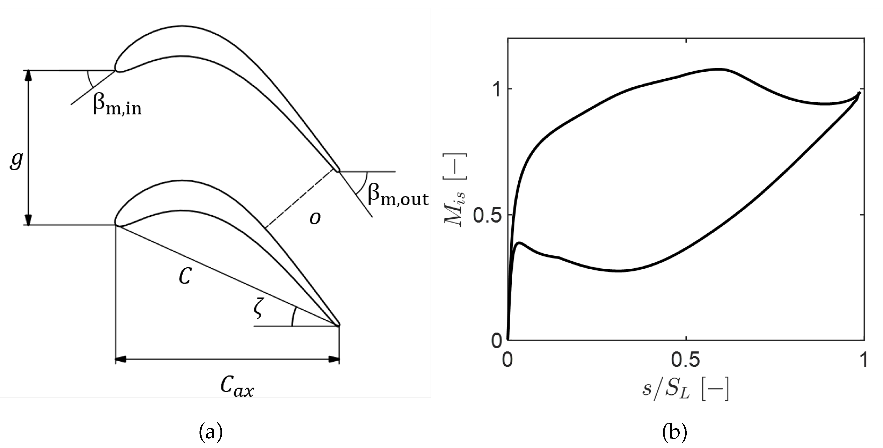
Figure 2.
The VKI S-1/C wind tunnel.
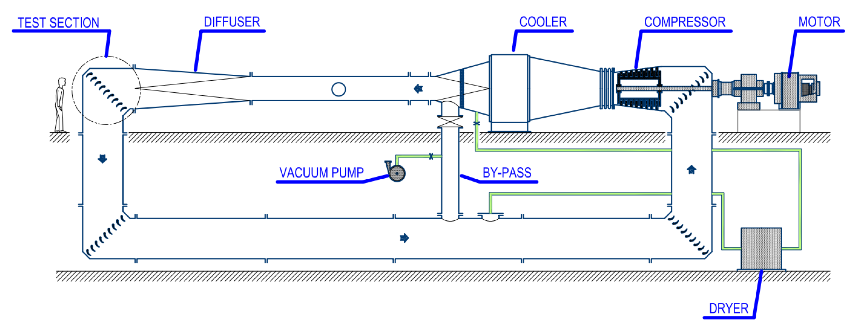
Figure 3.
Test section layout and instrumentation (a) and Blade-to-blade view (b).
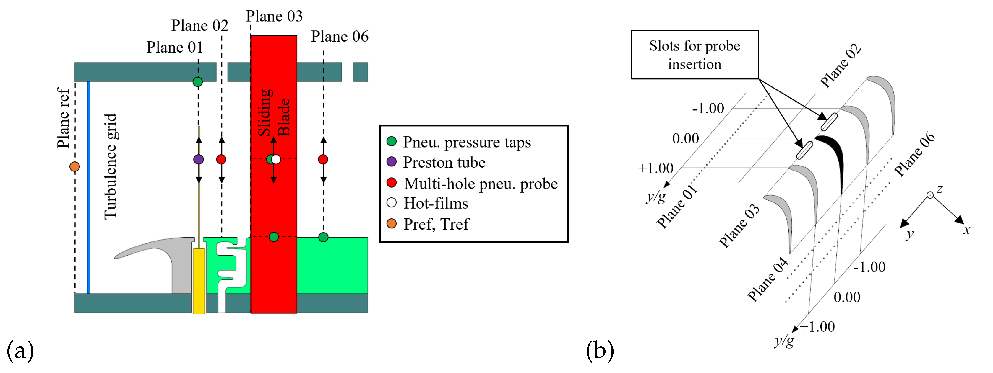
Figure 4.
Final meshes for MISES (a) and RANS (b).
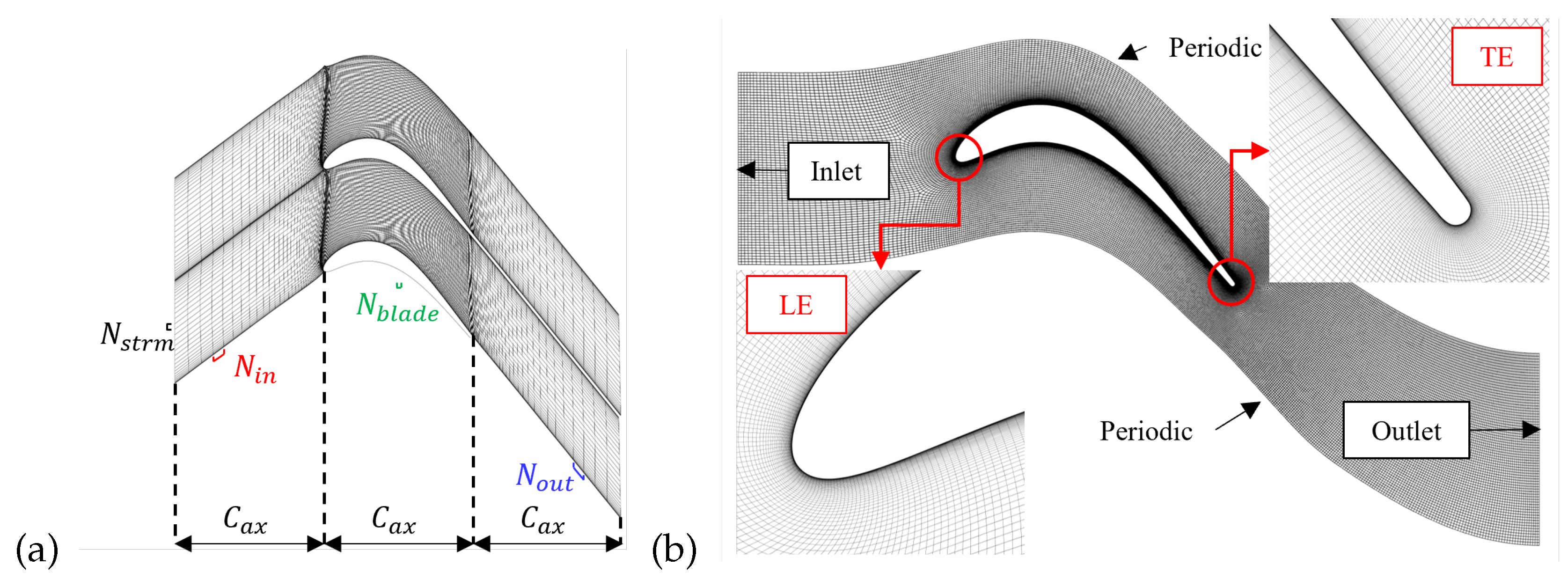
Figure 5.
RANS mesh sensitivity for and . (a) Surface isentropic Mach number along normalized surface length. (b) Mass-averaged total-pressure loss coefficient.
Figure 5.
RANS mesh sensitivity for and . (a) Surface isentropic Mach number along normalized surface length. (b) Mass-averaged total-pressure loss coefficient.
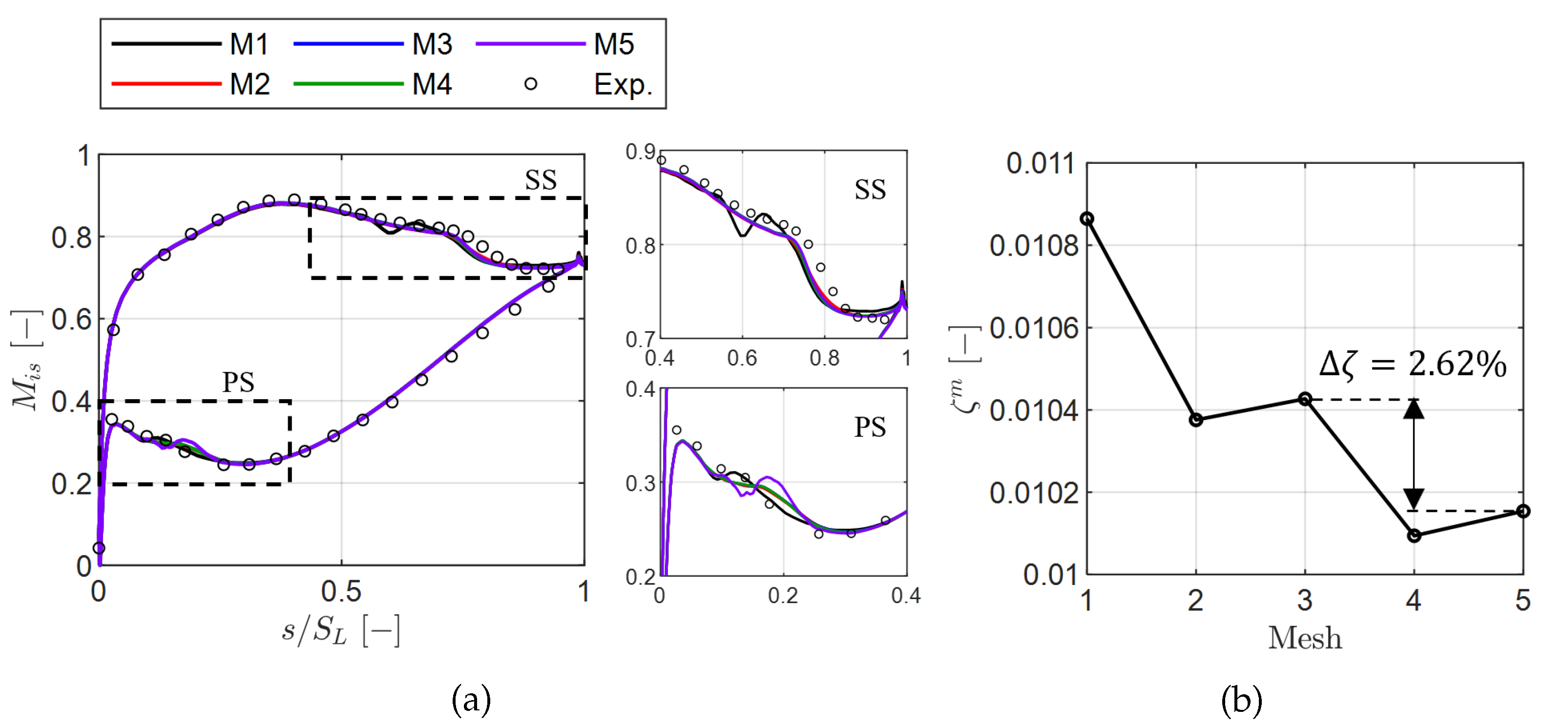
Figure 6.
Sensitivity to turbulence intensity. (a) Surface isentropic Mach number along the normalized surface length. (b) Relative error between MISES and experiments.
Figure 6.
Sensitivity to turbulence intensity. (a) Surface isentropic Mach number along the normalized surface length. (b) Relative error between MISES and experiments.
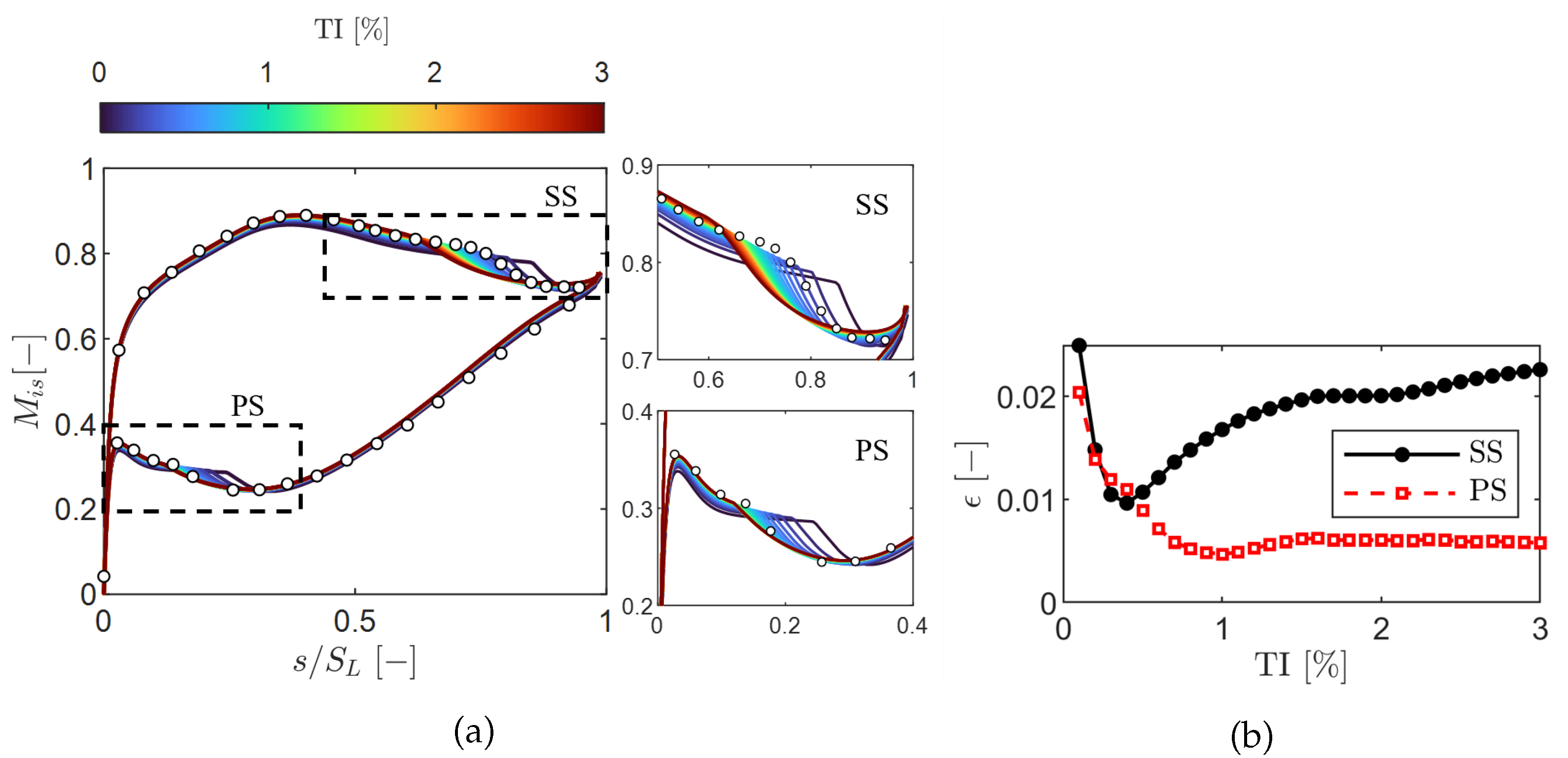
Figure 7.
RANS inlet turbulence decay tuned to cross-wire data and compared with the Roach correlation.
Figure 7.
RANS inlet turbulence decay tuned to cross-wire data and compared with the Roach correlation.
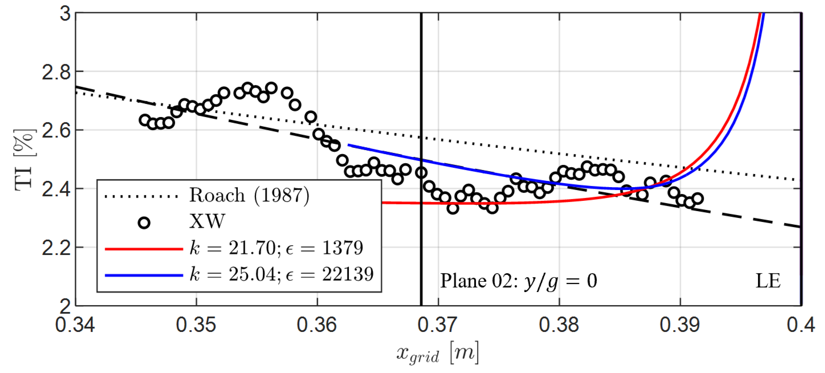
Figure 8.
Inlet boundary layer at Plane 01. (a) Spanwise for all conditions. (b) Spanwise mean with range (shaded).
Figure 8.
Inlet boundary layer at Plane 01. (a) Spanwise for all conditions. (b) Spanwise mean with range (shaded).
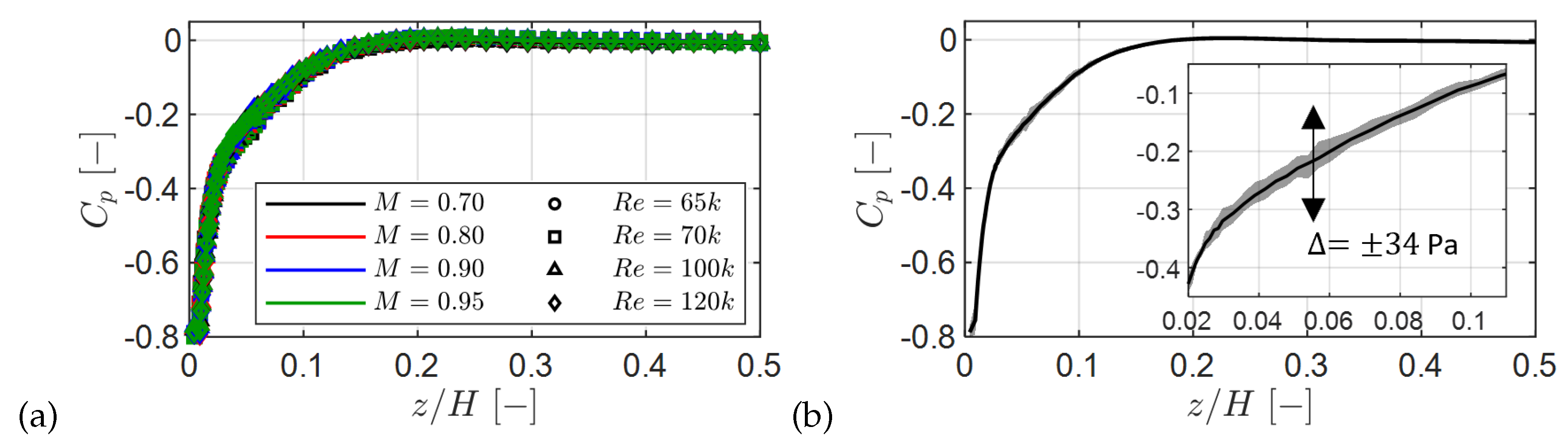
Figure 9.
Inlet boundary layer integral parameters versus operating point. (a) Displacement thickness. (b) Momentum thickness. (c) Shape factor.
Figure 9.
Inlet boundary layer integral parameters versus operating point. (a) Displacement thickness. (b) Momentum thickness. (c) Shape factor.
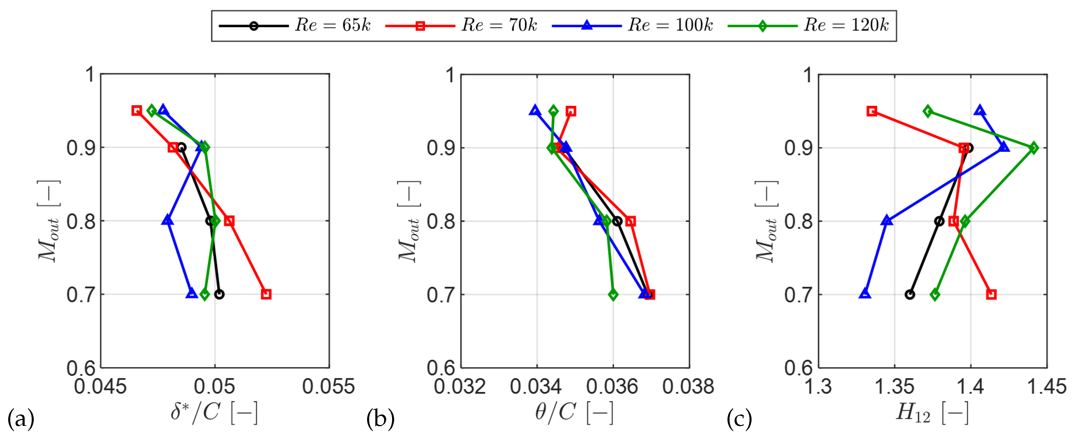
Figure 10.
Midspan inlet flow at Plane 02: (a) incidence, (b) cascade pitch angle, (c) normalized Mach number.
Figure 10.
Midspan inlet flow at Plane 02: (a) incidence, (b) cascade pitch angle, (c) normalized Mach number.
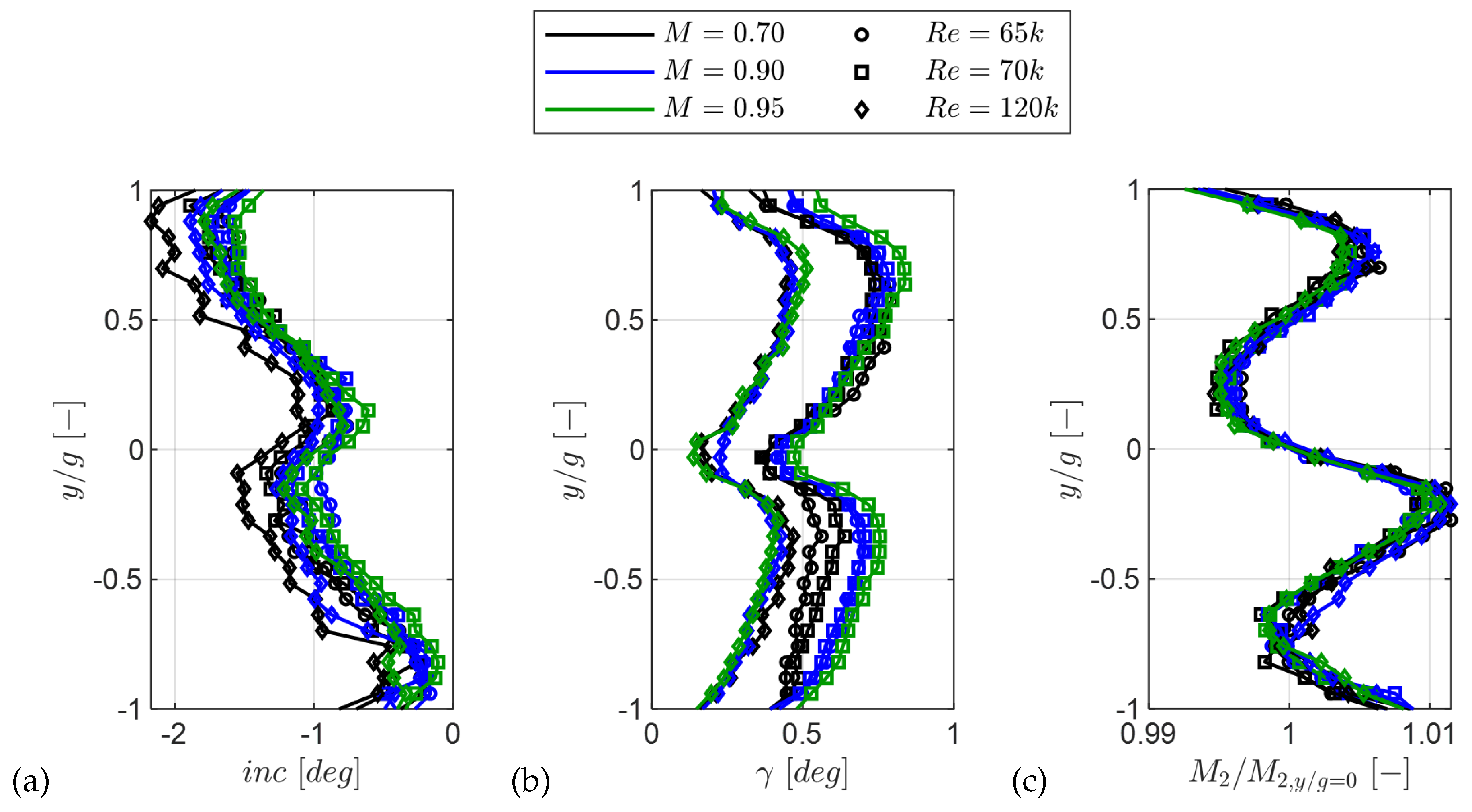
Figure 11.
Blade loading: experimental (markers), CFD (solid), and MISES AGS (dashed). (a), (b), (c), (d).
Figure 11.
Blade loading: experimental (markers), CFD (solid), and MISES AGS (dashed). (a), (b), (c), (d).
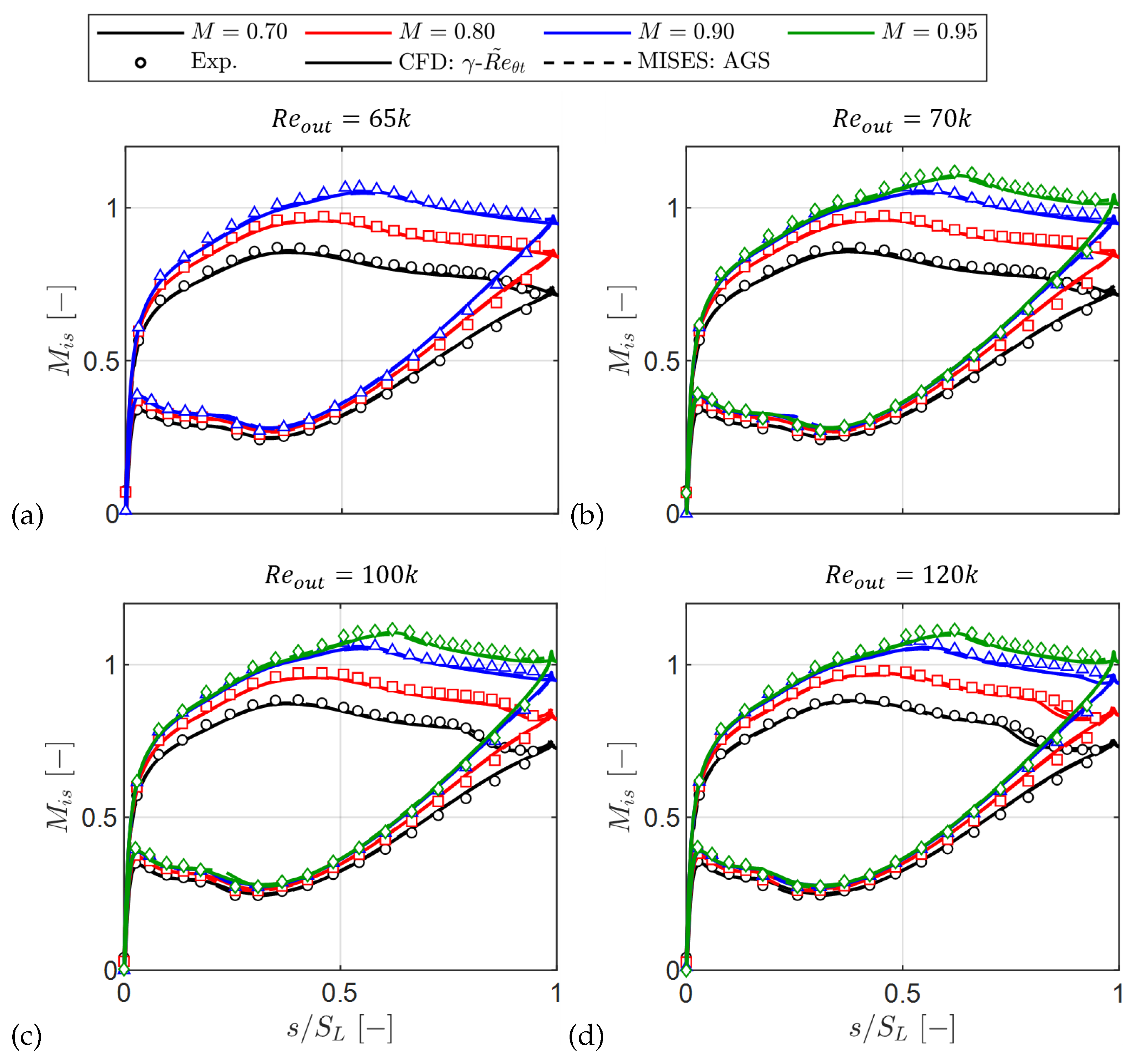
Figure 12.
Suction side close-up: experimental (markers), CFD (solid), and MISES AGS (dashed). (a), (b), (c), (d).
Figure 12.
Suction side close-up: experimental (markers), CFD (solid), and MISES AGS (dashed). (a), (b), (c), (d).
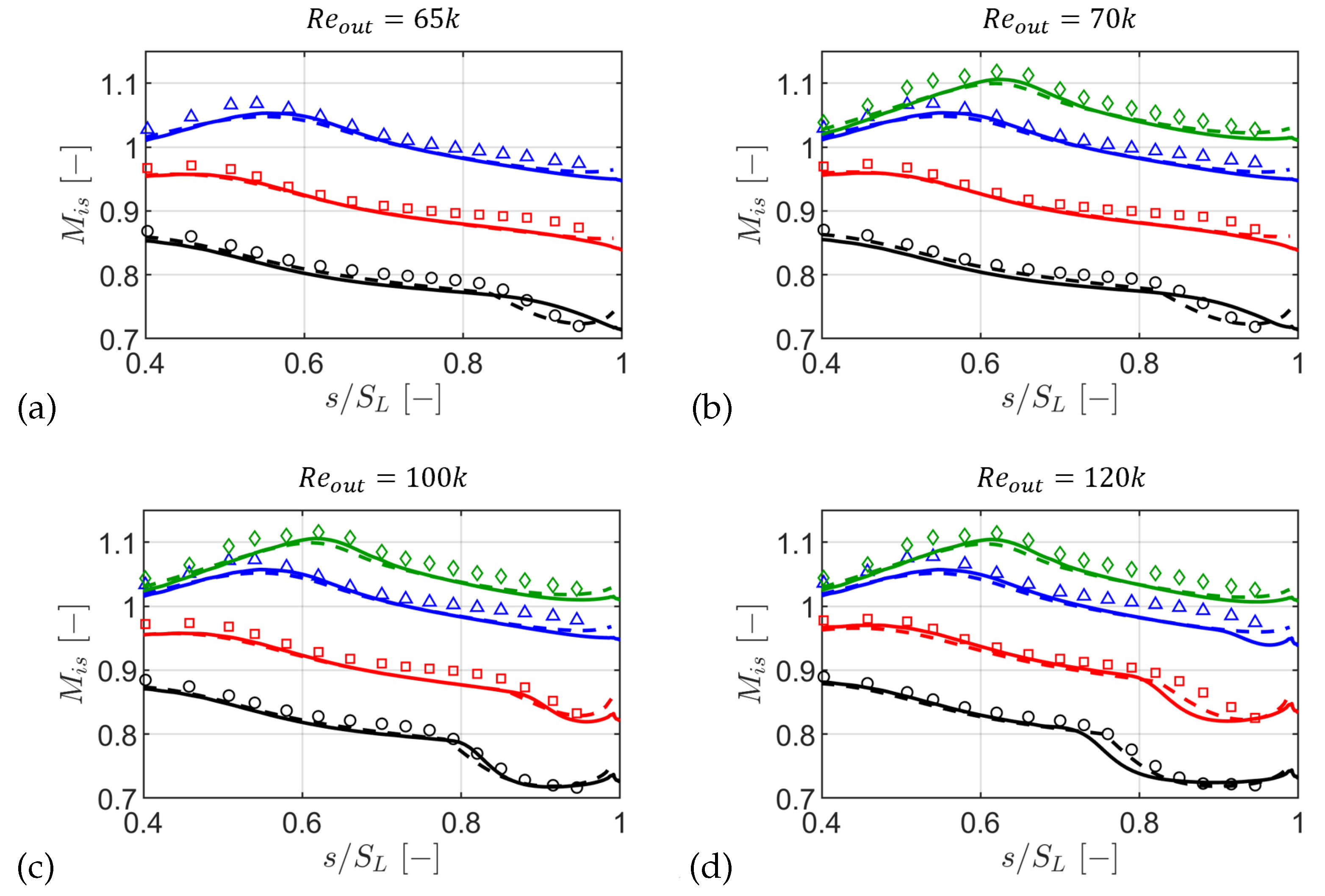
Figure 13.
Blade quasi-wall shear stress: experimental (markers), CFD (solid), and MISES AGS (dashed). Negative values are relative to the pressure side.
Figure 13.
Blade quasi-wall shear stress: experimental (markers), CFD (solid), and MISES AGS (dashed). Negative values are relative to the pressure side.
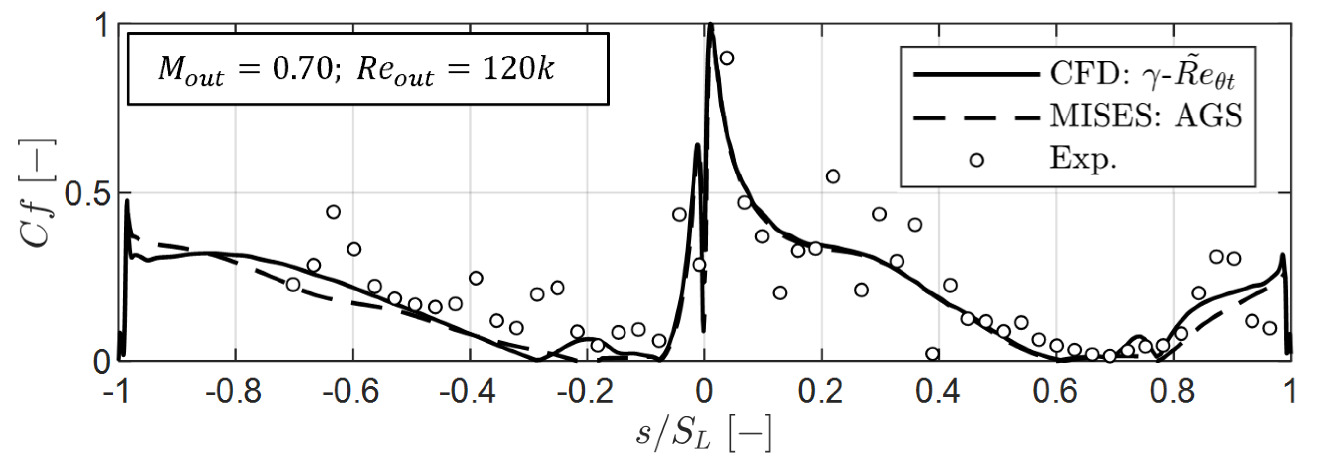
Figure 14.
Suction side (black, left axis), acceleration parameter (red, right axis), and scaled (blue, right axis). (a) and (b).
Figure 14.
Suction side (black, left axis), acceleration parameter (red, right axis), and scaled (blue, right axis). (a) and (b).
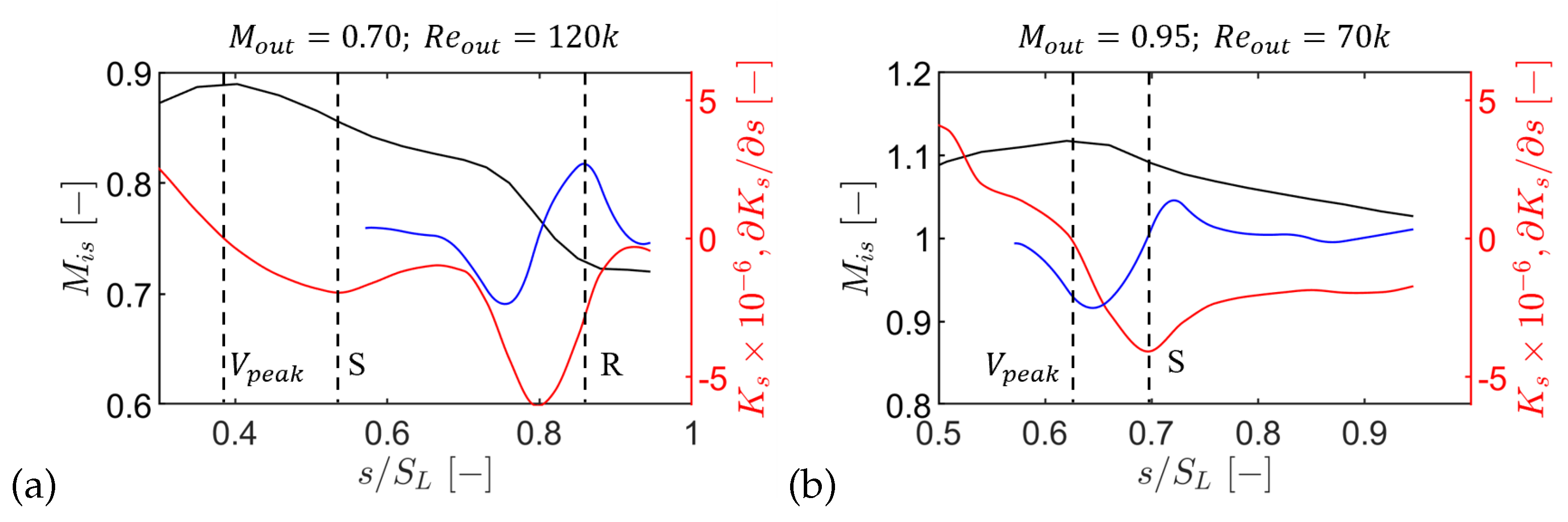
Figure 15.
Separation location from skin friction versus from the method. The shaded band indicates about the line.
Figure 15.
Separation location from skin friction versus from the method. The shaded band indicates about the line.
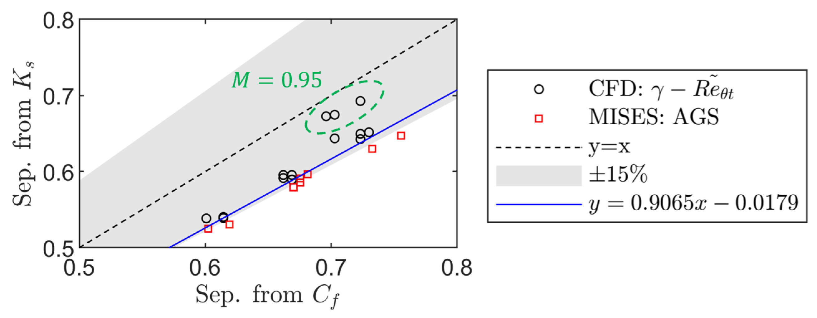
Figure 16.
Acceleration parameter at separation versus surface-length-based Reynolds number: without correction (a) and with separation-location correction (b).
Figure 16.
Acceleration parameter at separation versus surface-length-based Reynolds number: without correction (a) and with separation-location correction (b).
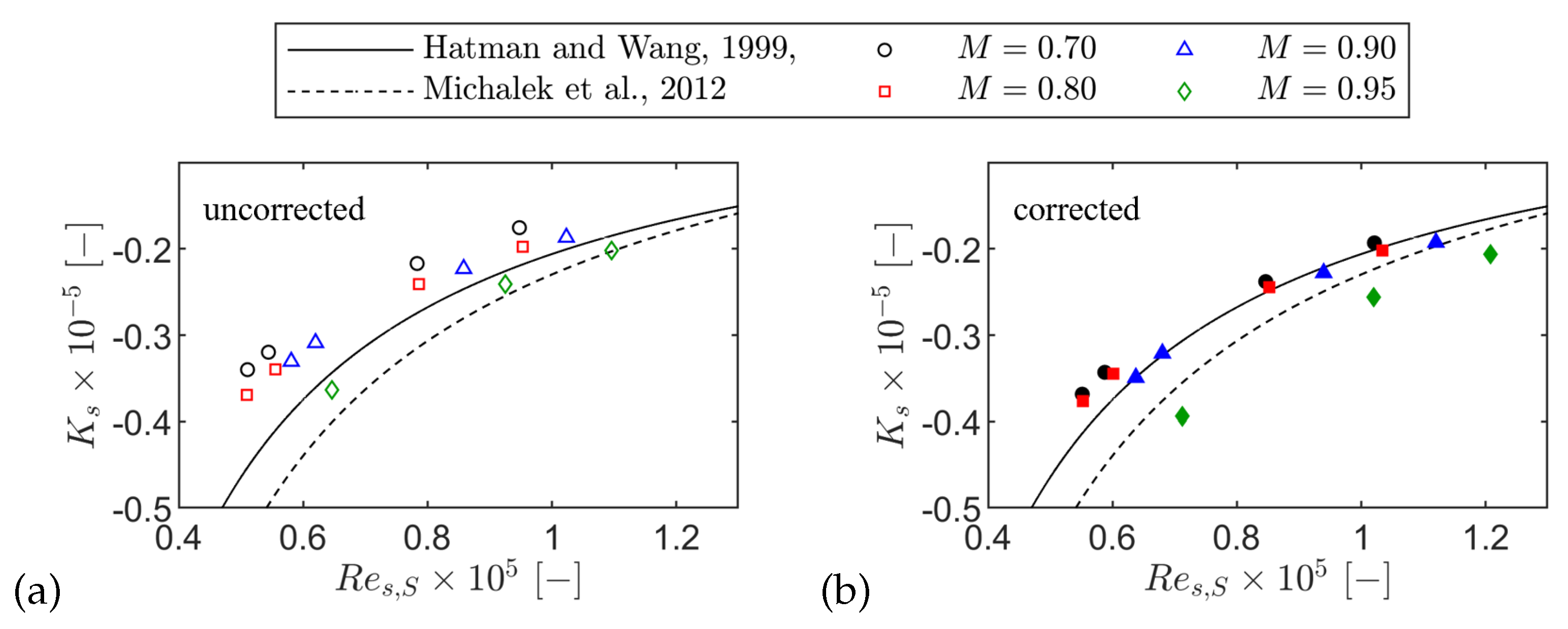
Figure 17.
Surface-length-based Reynolds number at reattachment versus at separation.
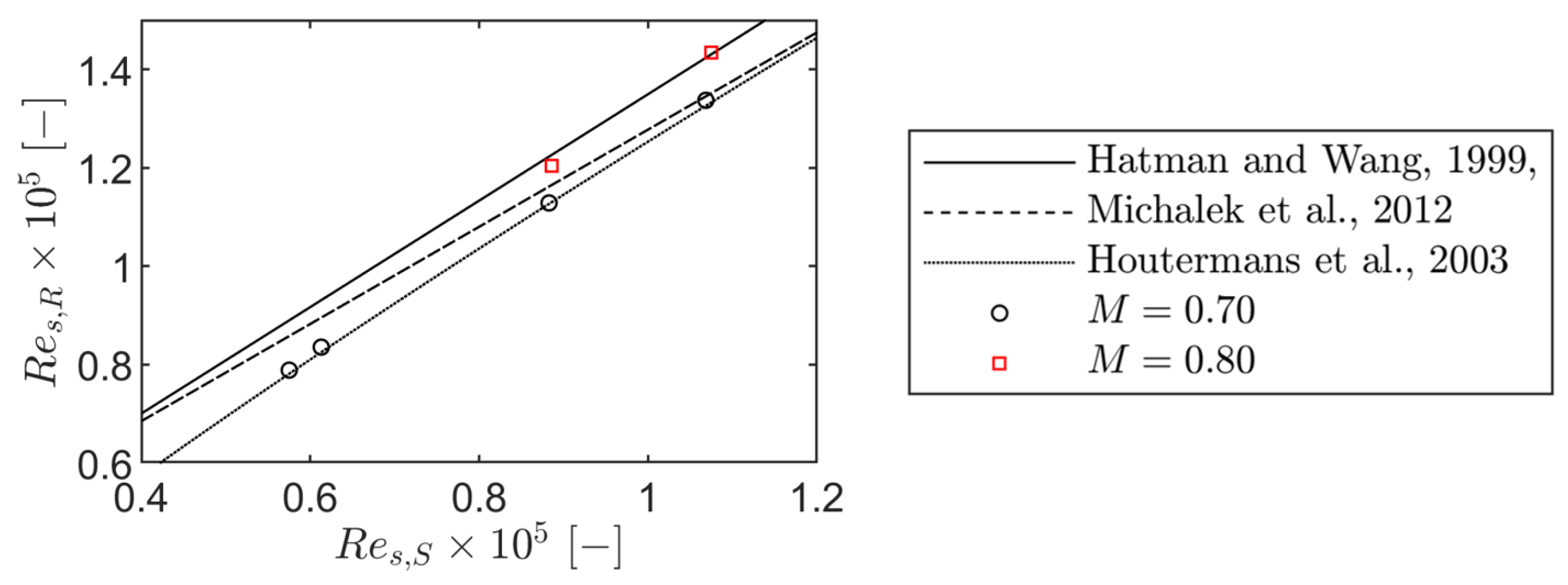
Figure 18.
Spanwise variation of blade loading: (a) and sensitivity of near-wall loading at to Reynolds number at (b).
Figure 18.
Spanwise variation of blade loading: (a) and sensitivity of near-wall loading at to Reynolds number at (b).
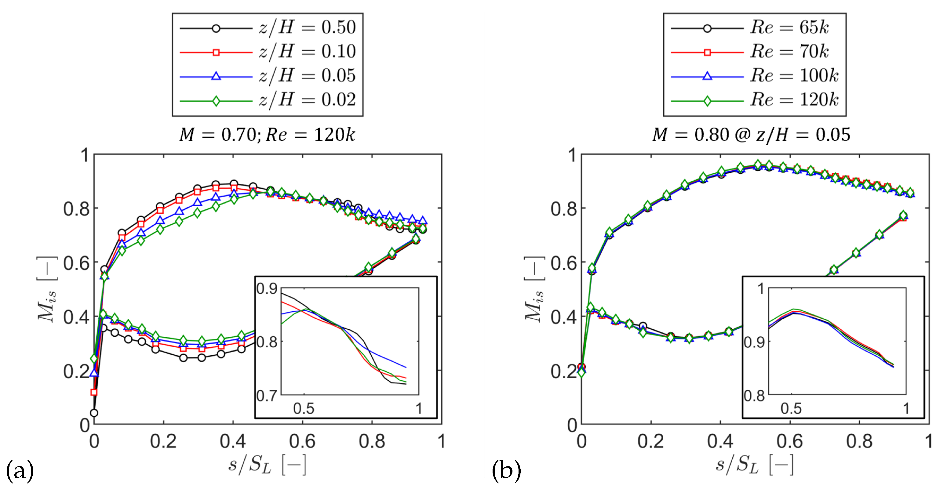
Figure 19.
Pitchwise distribution of kinetic energy loss coefficient: Re=70k (a) and Re=120k (b).
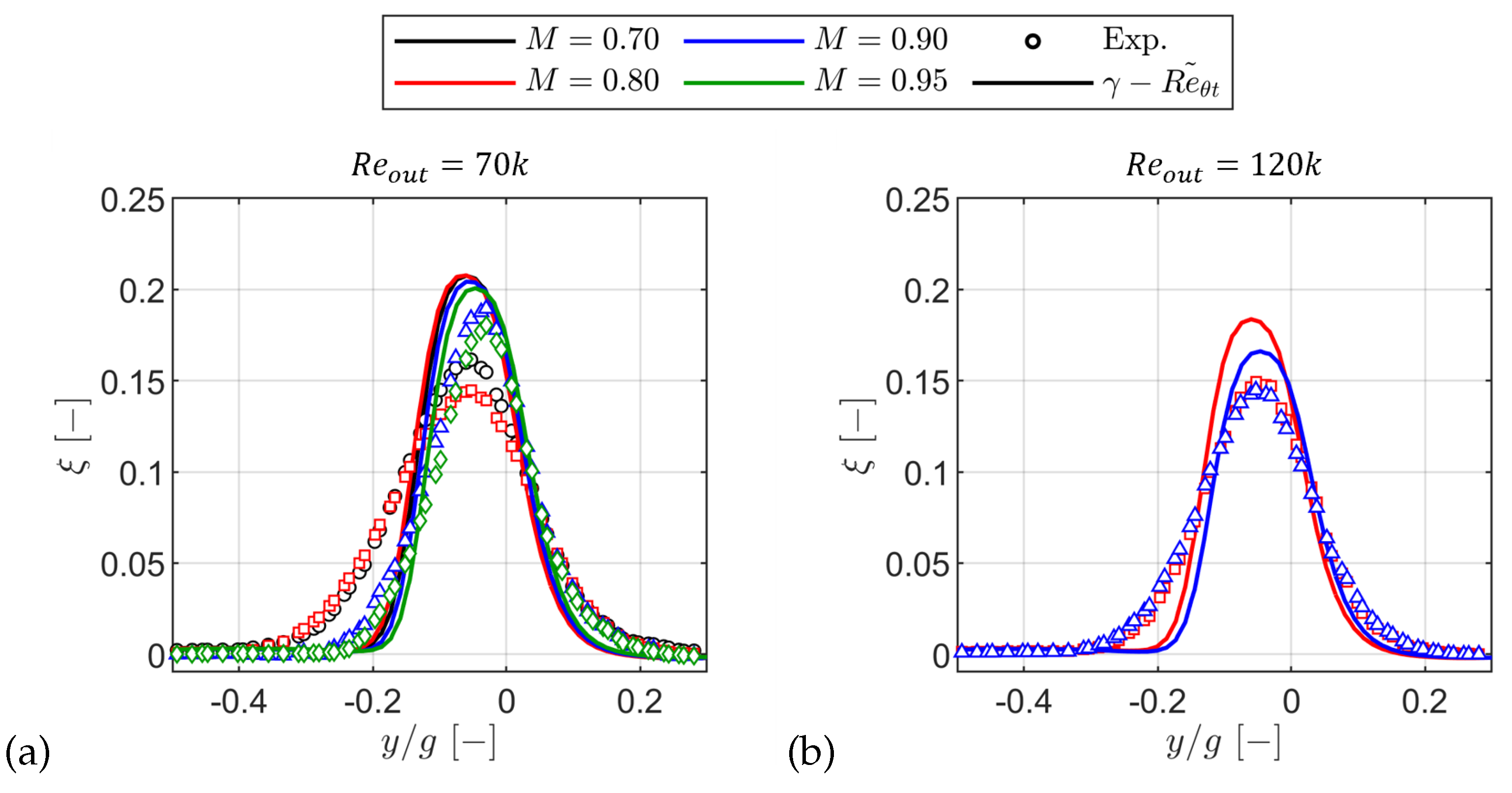
Figure 20.
Mass-averaged profile loss in terms of kinetic energy loss coefficient.
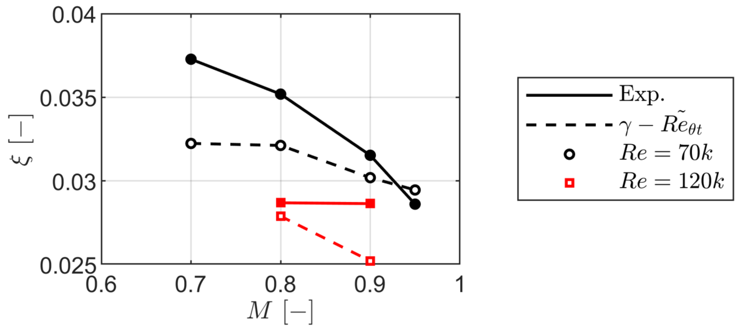
Figure 21.
Representation of primary and secondary flow structures with Q-criterion.
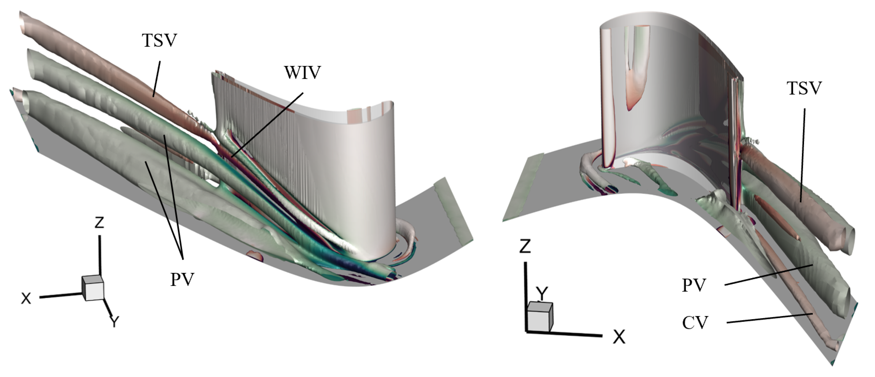
Figure 22.
Secondary flow structures at Plane 06 for nominal flow case: kinetic energy loss coefficient (a), streamwise vorticity coefficient superimposed with isolines of kinetic energy loss coefficient (b) and secondary kinetic energy coefficient superimposed with secondary velocity vectors (c). The observer looks upstream.
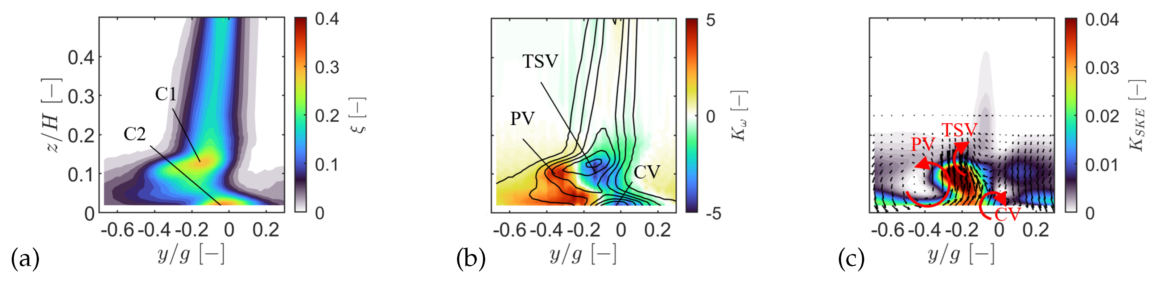
Figure 23.
Impact of Mach number at a Reynolds number of 70,000: M=0.70 (a), M=0.90 (b) and M=0.95 (c).
Figure 23.
Impact of Mach number at a Reynolds number of 70,000: M=0.70 (a), M=0.90 (b) and M=0.95 (c).
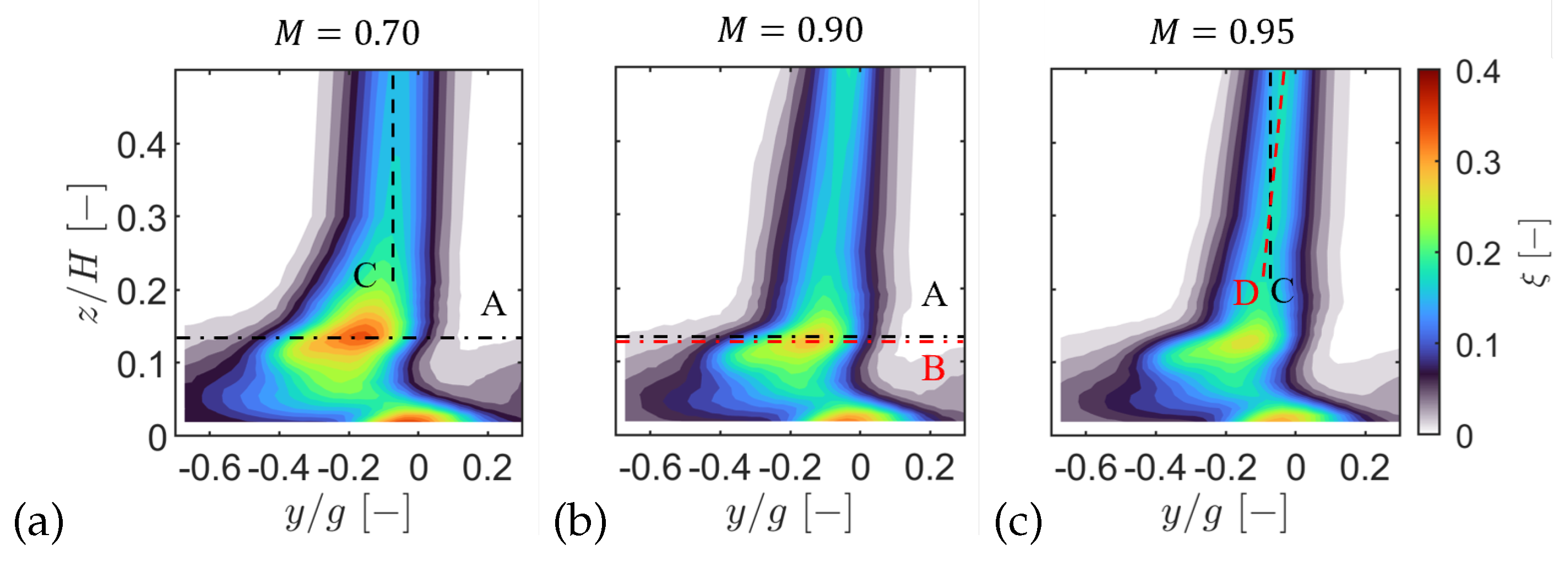
Figure 24.
Radial profiles for Re=70k: secondary kinetic energy loss coefficient (a), deviation from primary flow direction (b), and secondary kinetic energy coefficient (c).
Figure 24.
Radial profiles for Re=70k: secondary kinetic energy loss coefficient (a), deviation from primary flow direction (b), and secondary kinetic energy coefficient (c).
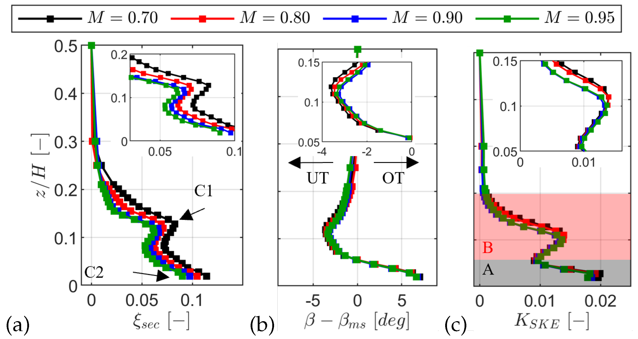
Figure 25.
Radial profiles for M=0.90: secondary kinetic energy loss coefficient (a), deviation from primary flow direction (b), and secondary kinetic energy coefficient (c).
Figure 25.
Radial profiles for M=0.90: secondary kinetic energy loss coefficient (a), deviation from primary flow direction (b), and secondary kinetic energy coefficient (c).
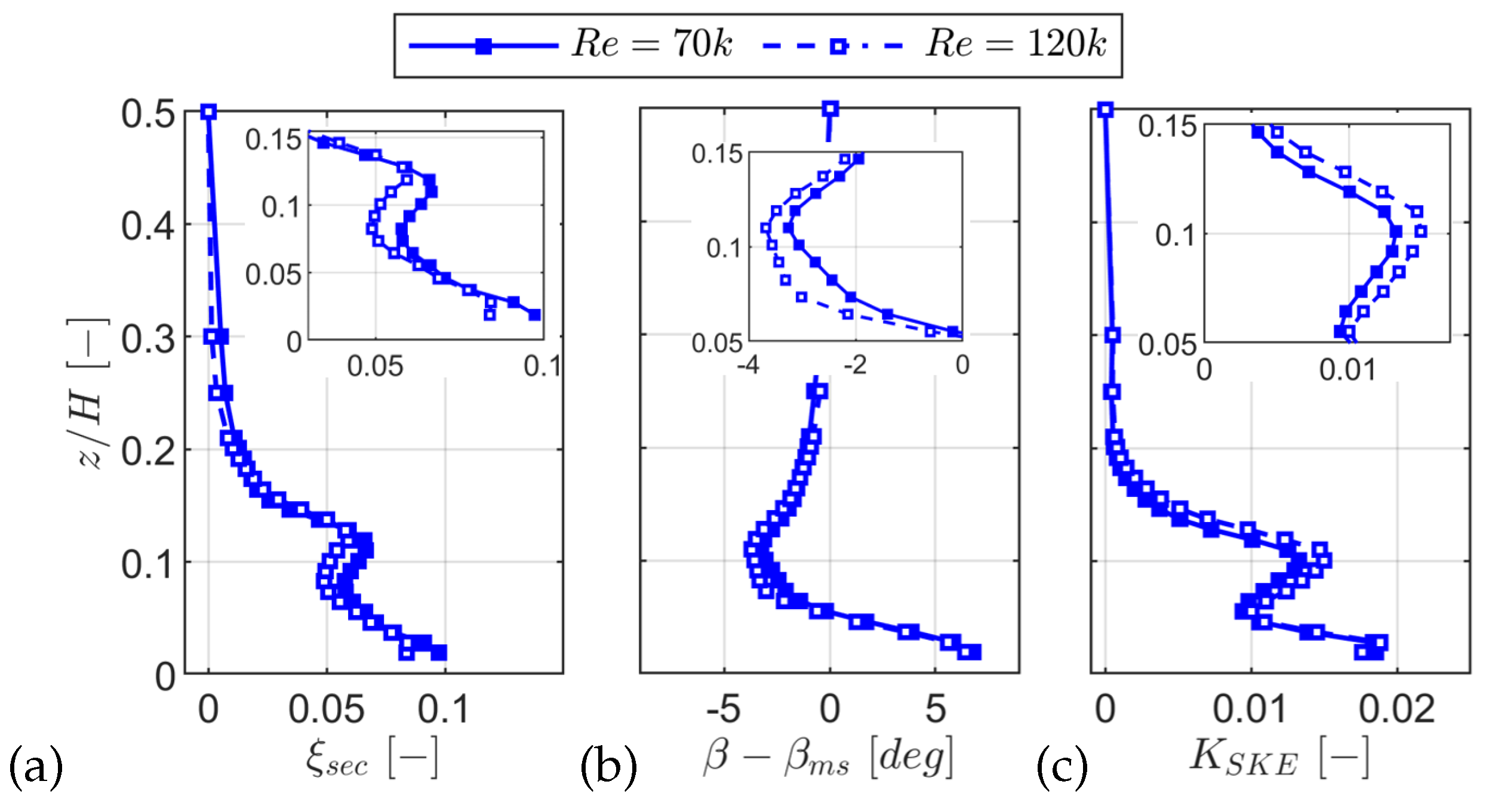
Figure 26.
Breakdown of the planewise mass-averaged losses for the steady inlet flow cases.
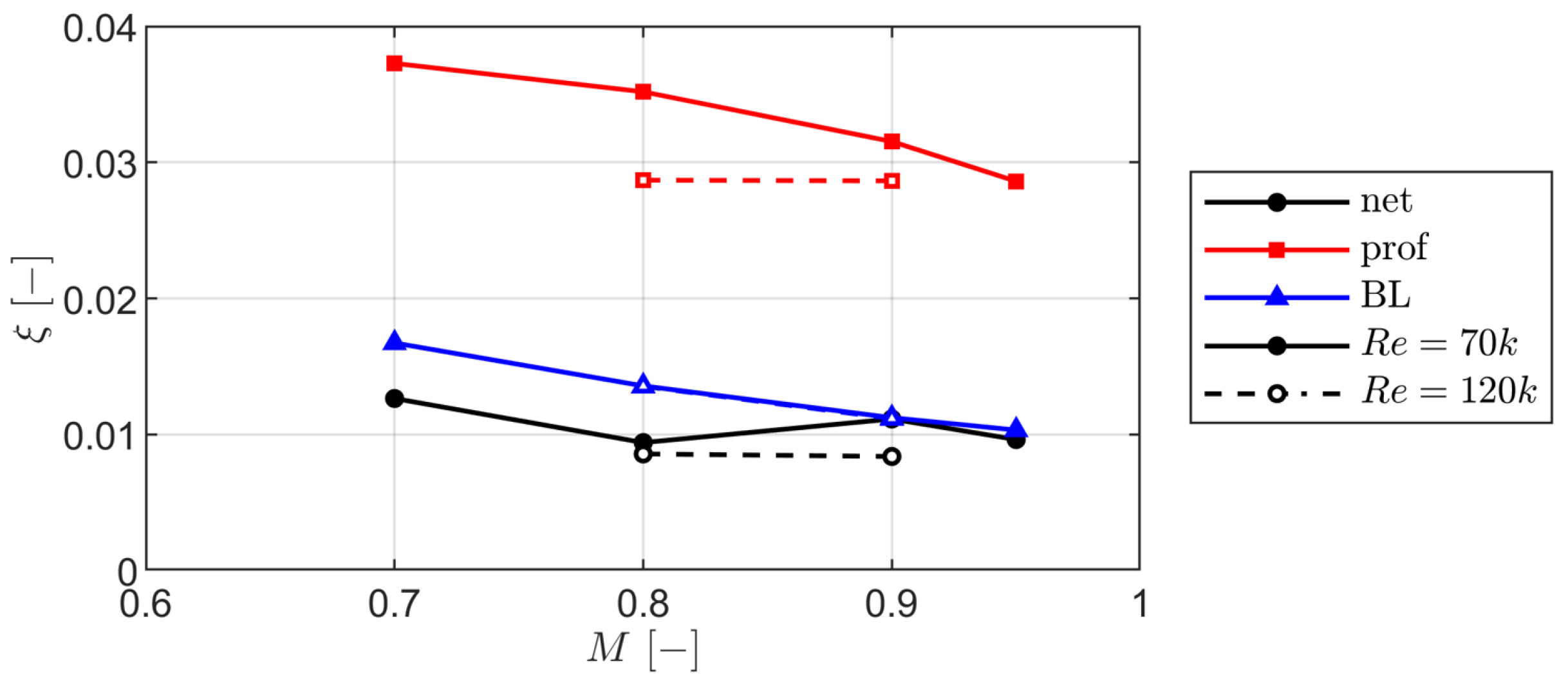
Figure 27.
Comparison of experimentally obtained separation locations against those estimated with different methods: Thwaites (a) and Stratford (b).
Figure 27.
Comparison of experimentally obtained separation locations against those estimated with different methods: Thwaites (a) and Stratford (b).
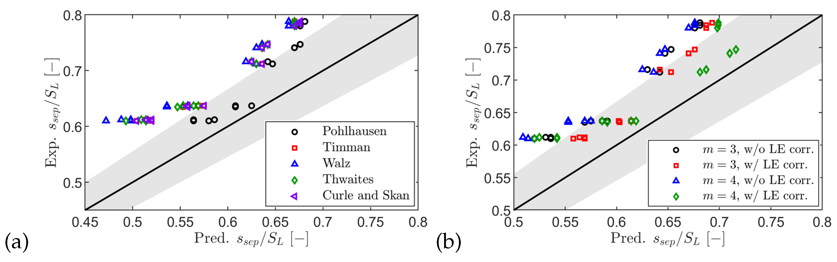
Figure 28.
Comparison of experimentally obtained separation location against the one estimated with the best method of the Thwaites and Stratford type methods.
Figure 28.
Comparison of experimentally obtained separation location against the one estimated with the best method of the Thwaites and Stratford type methods.
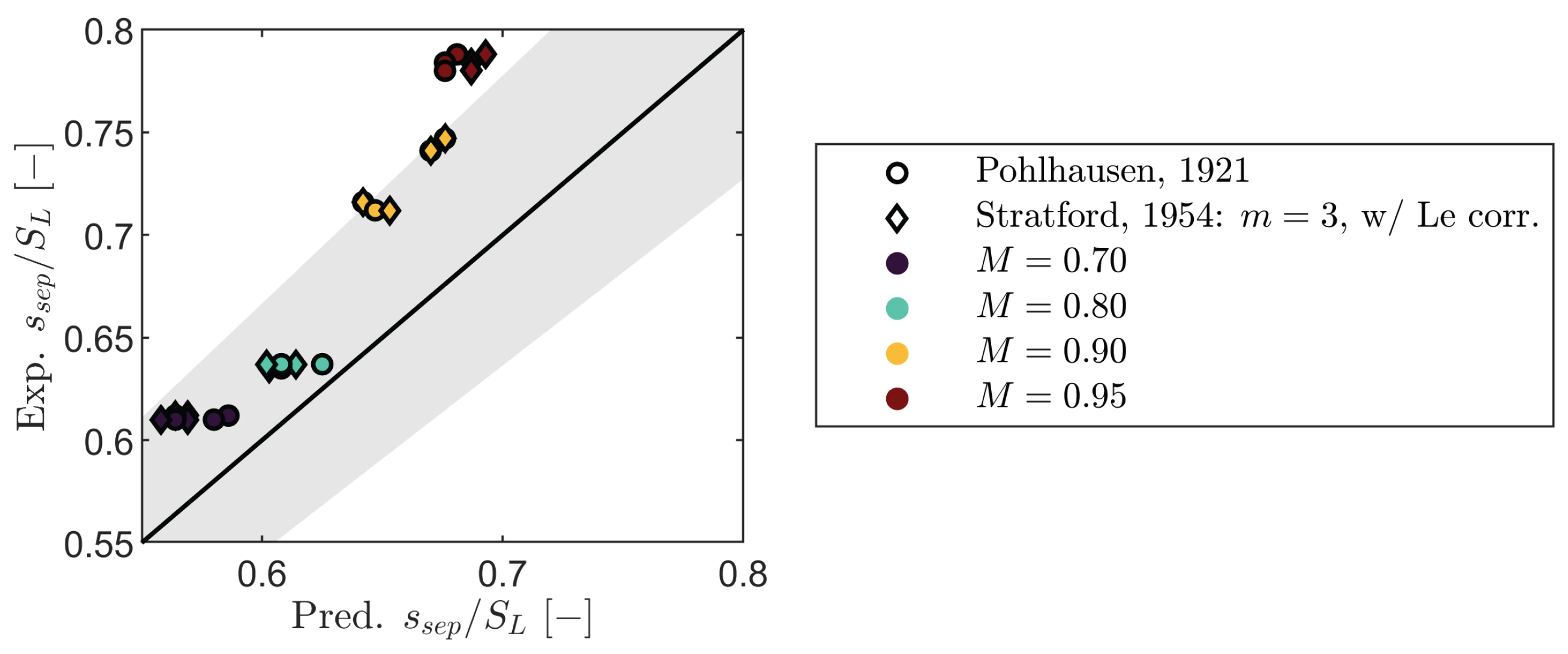
Figure 29.
Loss breakdown by flow condition (a), and contributions of BL on SS (b) for steady inlet flow cases.
Figure 29.
Loss breakdown by flow condition (a), and contributions of BL on SS (b) for steady inlet flow cases.
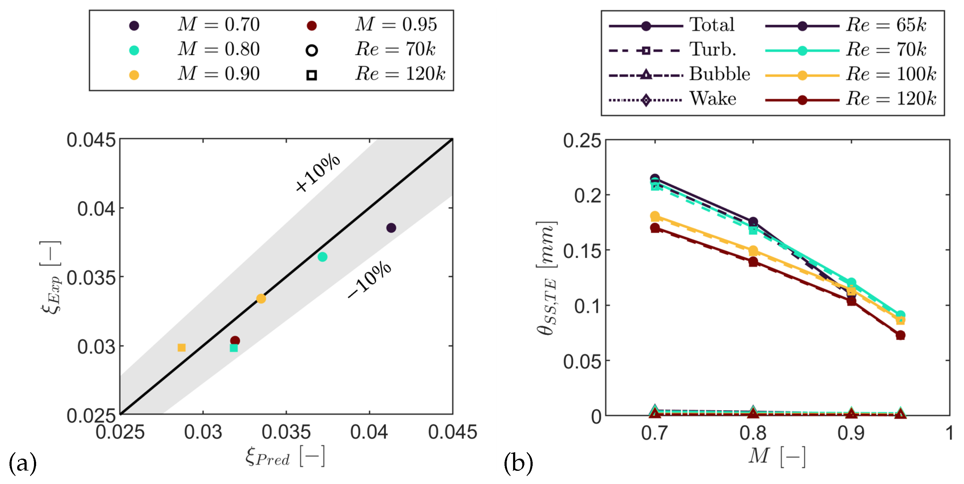
Figure 30.
Breakdown of loss contributions of profile loss from Equation 16–Equation 19: mixing loss (a), blockage loss (b), trailing edge wedge angle loss (c), and base pressure loss (d).
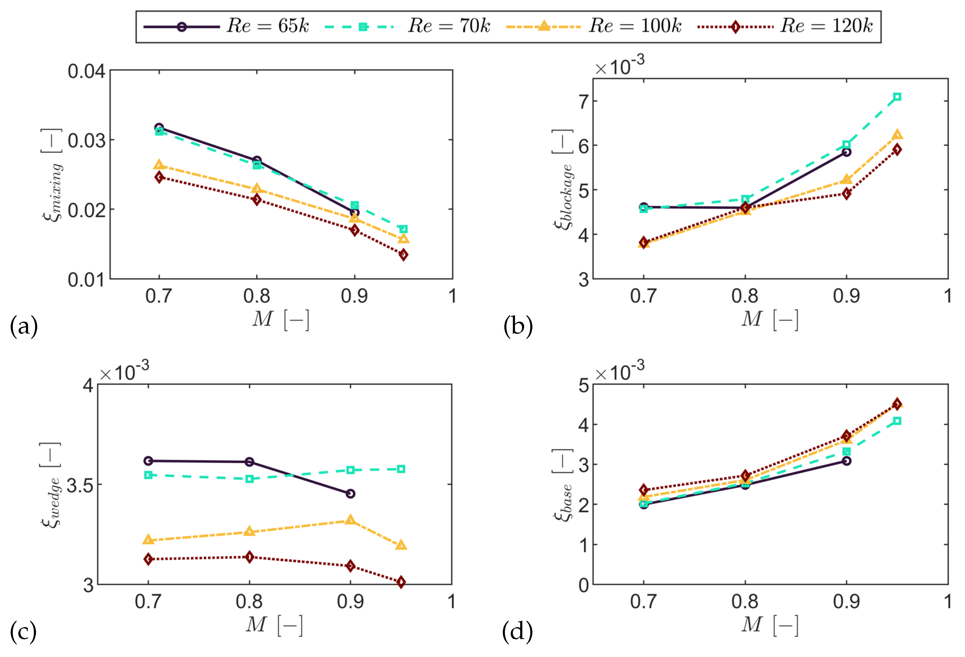
Figure 31.
Isentropic Mach number along the normalized axial direction (a) and endwall-loss integral using experimental versus MISES inputs (b). The loss integral is evaluated over the experimentally delimited area.
Figure 31.
Isentropic Mach number along the normalized axial direction (a) and endwall-loss integral using experimental versus MISES inputs (b). The loss integral is evaluated over the experimentally delimited area.
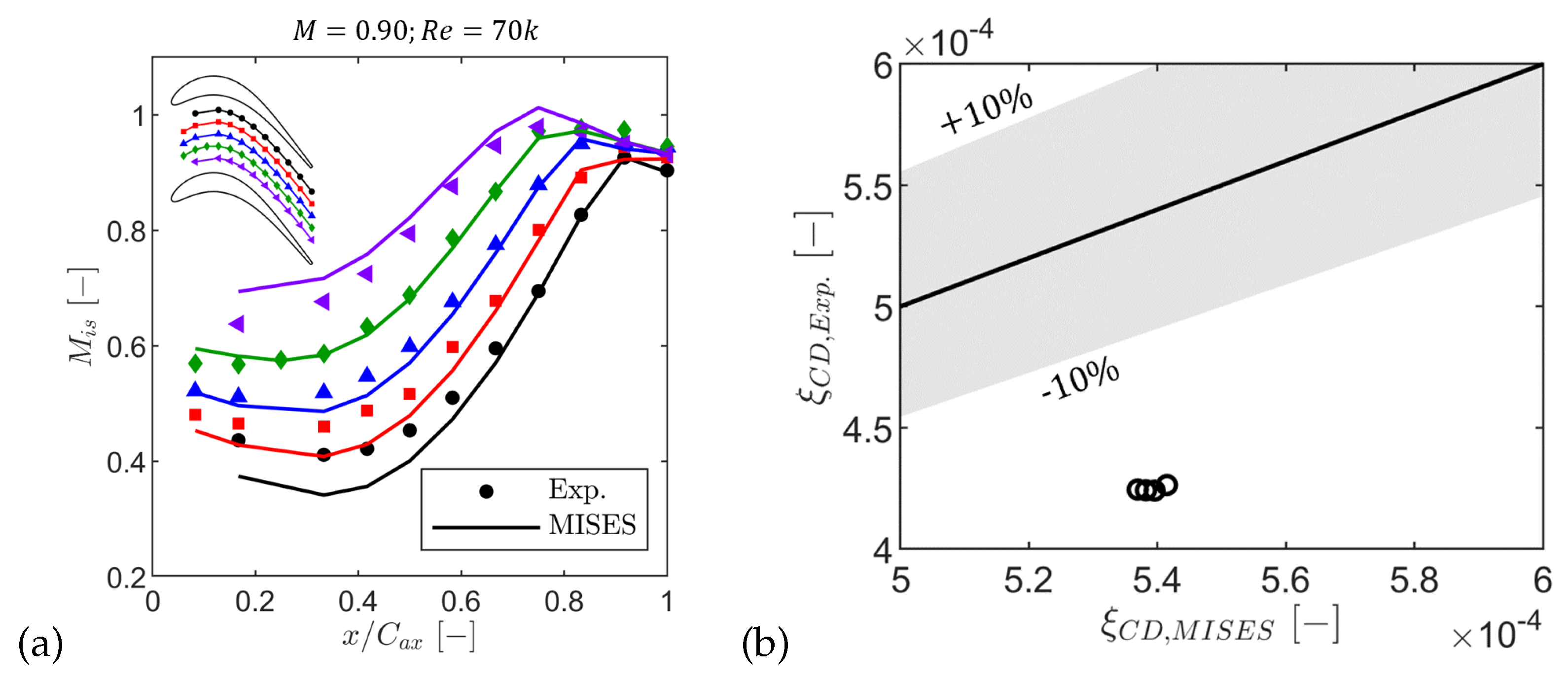
Figure 32.
Sensitivity of endwall loss to the Mach number and the Reynolds number using the model of Coull [34].
Figure 32.
Sensitivity of endwall loss to the Mach number and the Reynolds number using the model of Coull [34].
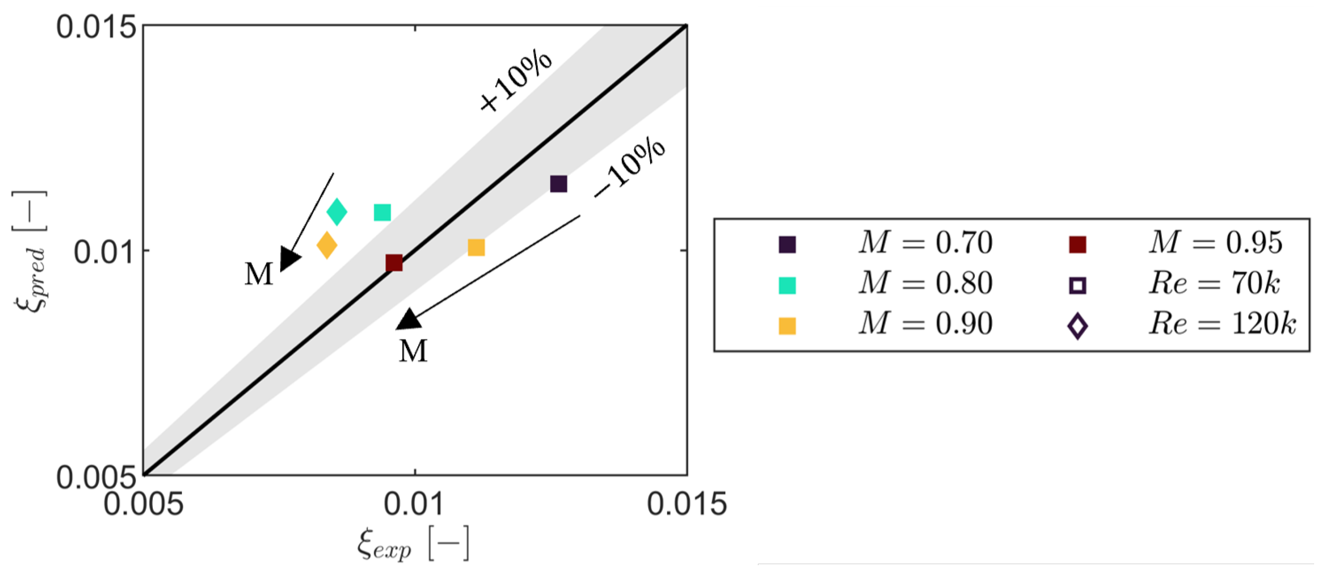
Figure 33.
Breakdown by secondary structure (a) and decomposition into endwall dissipation and mixing (b) for steady-flow cases.
Figure 33.
Breakdown by secondary structure (a) and decomposition into endwall dissipation and mixing (b) for steady-flow cases.
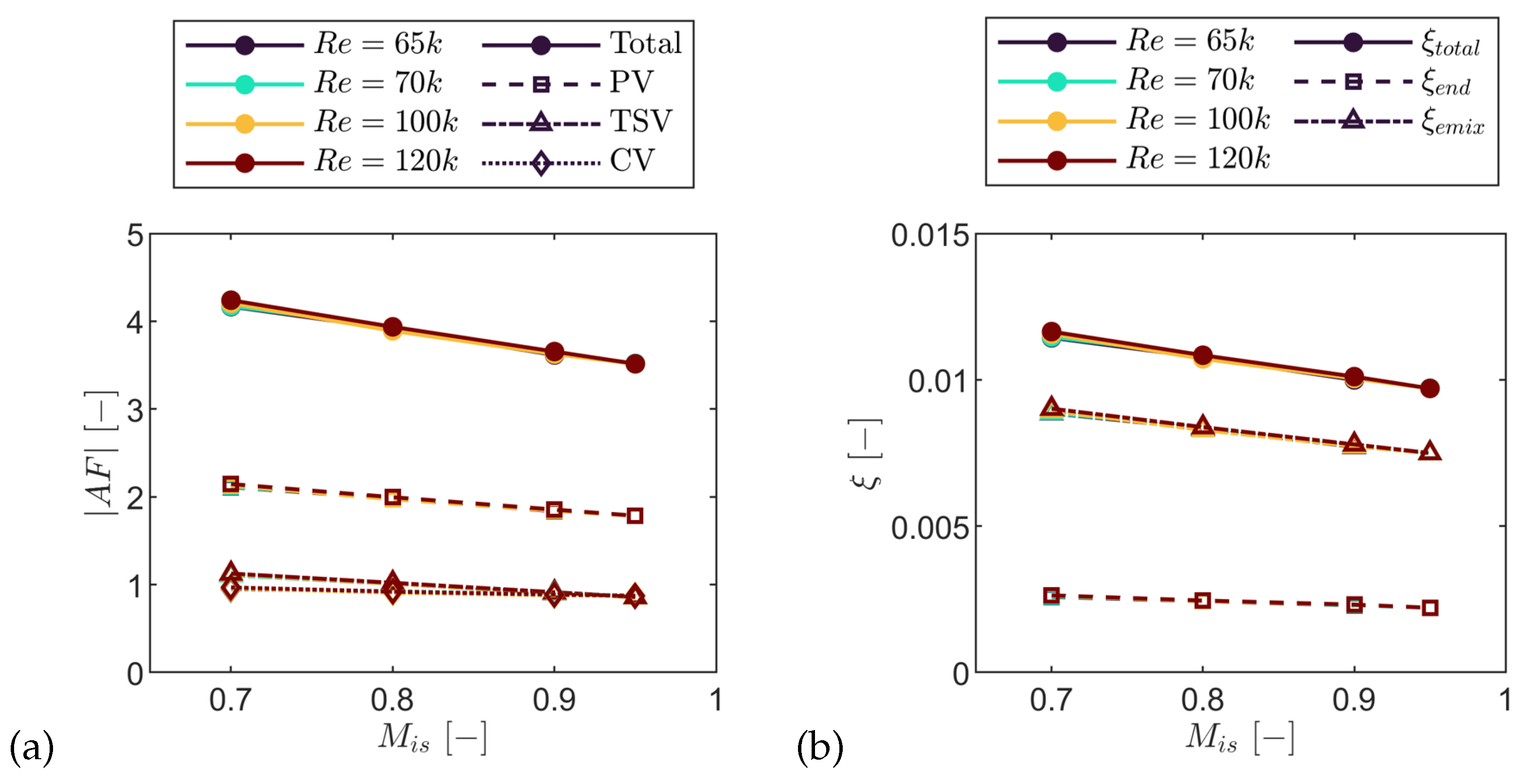
Figure 34.
Sensitivity of secondary kinetic energy to Mach and Reynolds numbers using the model of Coull [57].
Figure 34.
Sensitivity of secondary kinetic energy to Mach and Reynolds numbers using the model of Coull [57].
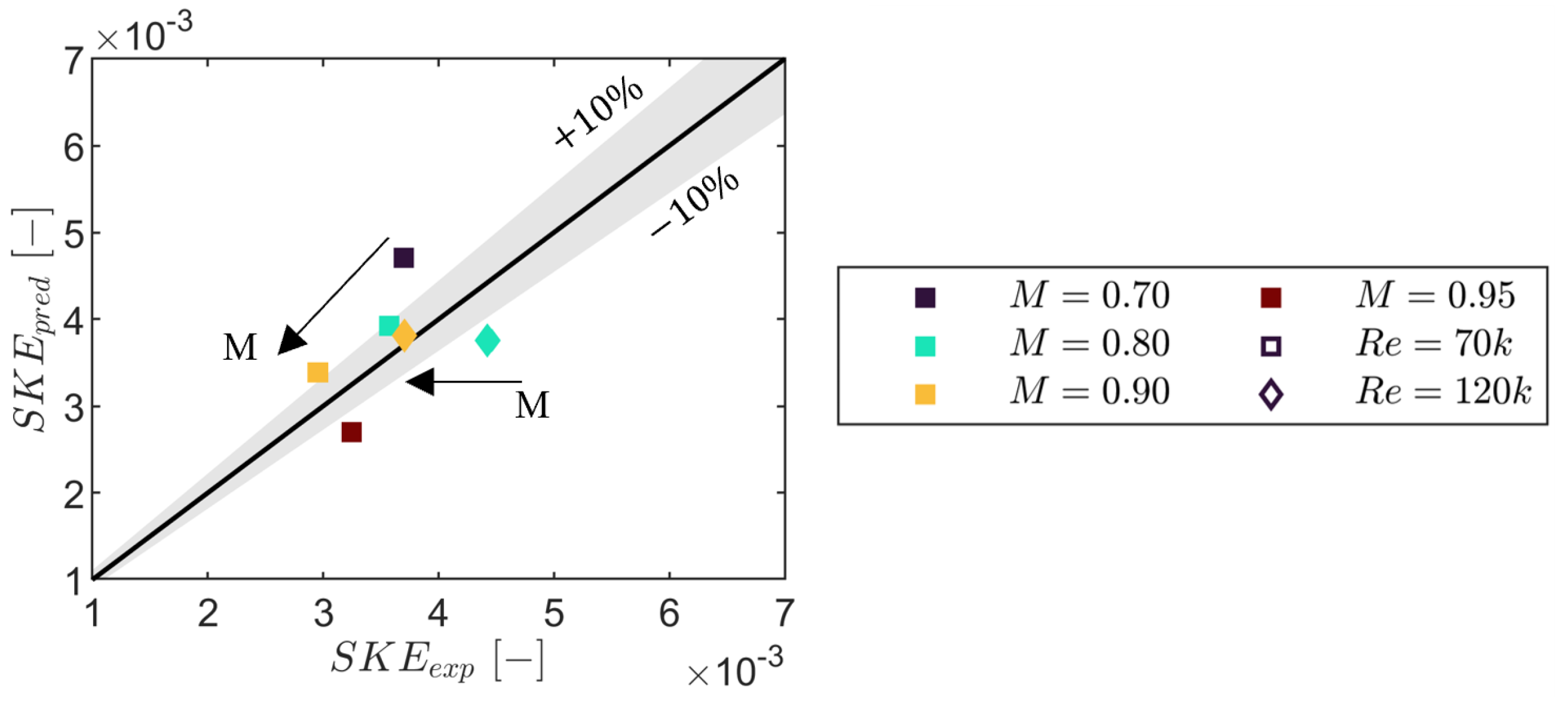

Table 1.
SPLEEN C1 cascade key geometrical features.
| True chord, C | 52.285 | [] |
| Axial chord, | 47.614 | [] |
| Pitch-to-chord ratio, | 0.630 | [−] |
| Cascade span, H | 165 | [] |
| TE thickness, | 0.86 | [] |
| TE radius/C | 0.0082 | [−] |
| TE wedge angle | 4.96 | [∘] |
| Throat, o | 19.400 | [] |
| Inlet metal angle, | 37.30 | [∘] |
| Outlet metal angle, | 53.80 | [∘] |
| Stagger angle, | 24.40 | [∘] |
| Diffusion factor, DF | 18 | [%] |
| Circulation coefficient, C0 | 0.61 | [−] |
| Zweifel coefficient, | 0.73 | [−] |
Table 2.
Breakdown of experimental uncertainty with 95% confidence interval.
| Instrument | Qt. | Unit | ||
| Fixed | K | 0.01 | 0.52 | |
| Pa | 7.01 | 29.82 | ||
| Blade pneu./Endwall pneu. | − | 0.001 | 0.005 | |
| Preston tube | − | 0.001 | 0.008 | |
| C5HP | ∘ | 0.31 | 0.98 | |
| M | − | 0.002 | 0.010 | |
| L5HP | - | ∘ | 0.15 | 0.33 |
| − | 0.002 | 0.010 |
Table 3.
Instrumentation by operating condition. AP: aerodynamic probes. BP: blade pneumatic taps. EP: endwall pneumatic taps. HF: hot films.
Table 3.
Instrumentation by operating condition. AP: aerodynamic probes. BP: blade pneumatic taps. EP: endwall pneumatic taps. HF: hot films.
| 0.70 | 0.80 | 0.90 | 0.95 | ||
| 65,000 | BP/EP | BP | BP/EP | BP | |
| 70,000 | AP/BP/HF | AP/BP | AP/BP/HF/EP | AP/BP/HF/EP | |
| 100,000 | BP | BP | BP/EP | BP/EP | |
| 120,000 | BP/HF | AP/BP | AP/BP/HF/EP | BP | |
Table 4.
Mesh parameters for MISES computations.
| Total elements | ||||
|---|---|---|---|---|
| 40 | 40 | 40 | 200 | 10,803 |
Table 5.
RANS meshes for the sensitivity study.
| Name | Max. ER | Max. | |||
|---|---|---|---|---|---|
| M1 | 137 | 121 | ∼50,000 | 1.20 | 1.02 |
| M2 | 177 | 157 | ∼80,000 | 1.20 | 0.64 |
| M3 | 209 | 189 | ∼115,000 | 1.20 | 0.38 |
| M4 | 241 | 213 | ∼150,000 | 1.20 | 0.26 |
| M5 | 261 | 229 | ∼180,000 | 1.20 | 0.13 |
Table 6.
RANS inlet turbulence parameters matching the experimental decay.
| 0.70 | 20.396 | 16275 | 2.60 | 0.93 | |
| 0.80 | 23.585 | 20237 | 2.63 | 0.93 | |
| 0.90 | 24.991 | 22074 | 2.63 | 0.93 | |
| 0.70 | 20.733 | 16680 | 2.62 | 0.93 | |
| 0.80 | 23.656 | 20329 | 2.63 | 0.93 | |
| 0.90 | 25.067 | 22175 | 2.62 | 0.93 | |
| 0.95 | 25.086 | 22200 | 2.60 | 0.93 | |
| 0.70 | 21.269 | 17331 | 2.63 | 0.93 | |
| 0.80 | 23.719 | 20410 | 2.63 | 0.93 | |
| 0.90 | 25.271 | 22446 | 2.63 | 0.93 | |
| 0.95 | 25.486 | 22733 | 2.63 | 0.93 | |
| 0.70 | 21.585 | 17718 | 2.65 | 0.93 | |
| 0.80 | 24.066 | 20859 | 2.64 | 0.93 | |
| 0.90 | 25.370 | 22578 | 2.62 | 0.93 | |
| 0.95 | 25.600 | 22885 | 2.61 | 0.93 |
Table 7.
Separation location, , from experiments, CFD, and MISES under steady inlet flow.
| Exp. | ||||||||
|---|---|---|---|---|---|---|---|---|
| from | from | CFD | MISES | |||||
| 65,000 | 0.70 | 0.612 | - | - | 0.614 | 0.21 | 0.619 | 0.68 |
| 0.80 | 0.637 | - | - | 0.669 | 3.17 | 0.681 | 4.41 | |
| 0.90 | 0.747 | - | - | 0.730 | -1.67 | - | - | |
| 70,000 | 0.70 | 0.610 | 0.601 | -1.53 | 0.614 | 0.42 | 0.619 | 0.89 |
| 0.80 | 0.637 | 0.662 | 2.49 | 0.676 | 3.84 | |||
| 0.90 | 0.741 | 0.752 | 1.55 | 0.723 | -1.73 | - | - | |
| 100,000 | 0.70 | 0.612 | - | - | 0.601 | -1.15 | 0.602 | -1.00 |
| 0.80 | 0.635 | - | - | 0.669 | 3.37 | 0.676 | 4.04 | |
| 0.90 | 0.716 | - | - | 0.703 | -1.29 | 0.756 | 3.99 | |
| 120,000 | 0.70 | 0.610 | 0.601 | -1.53 | 0.614 | 0.42 | 0.602 | -0.79 |
| 0.80 | 0.637 | - | - | 0.662 | 2.49 | 0.670 | 3.27 | |
| 0.90 | 0.712 | 0.691 | -2.89 | 0.723 | 1.16 | 0.733 | 2.10 | |
Table 8.
Reattachment location, , from experiments, CFD, and MISES.
| Exp. | ||||||||
|---|---|---|---|---|---|---|---|---|
| from | from | CFD | MISES | |||||
| 65,000 | 0.70 | 0.931 | - | - | 0.985 | 5.46 | 0.848 | -8.23 |
| 70,000 | 0.70 | 0.921 | - | - | 0.972 | 5.12 | 0.837 | -8.45 |
| 100,000 | 0.70 | 0.871 | - | - | 0.852 | -1.84 | 0.802 | -6.86 |
| 0.80 | 0.932 | - | - | 0.915 | -1.75 | 0.854 | -7.86 | |
| 120,000 | 0.70 | 0.858 | 0.873 | 1.800 | 0.771 | -8.68 | 0.773 | -8.44 |
| 0.80 | 0.921 | - | - | 0.845 | -7.58 | 0.831 | -9.05 | |
Table 9.
Constants for the Thwaites–parameter separation criteria.
| Model | Const. |
|---|---|
| Pohlhausen [50] | -0.1567 |
| Timman [51] | -0.0871 |
| Walz [54] | -0.0682 |
| Thwaites [55] | -0.0820 |
| Curle and Skan [52] | -0.0900 |
Table 10.
Constants for the Stratford–type separation criteria.
| Model | Const. |
|---|---|
| Stratford [53], | 0.0108 |
| Stratford [53], | 6.48×10⁻³ |
Table 11.
Summary of blade loading parameters.
| 0.70 | 65,000 | 0.95 | 25 | 0.35 | 0.82 |
| 0.80 | 65,000 | 0.95 | 20 | 0.33 | 0.78 |
| 0.90 | 65,000 | 0.95 | 18 | 0.35 | 0.73 |
| 0.70 | 70,000 | 0.94 | 25 | 0.35 | 0.82 |
| 0.80 | 70,000 | 0.95 | 21 | 0.34 | 0.78 |
| 0.90 | 70,000 | 0.97 | 18 | 0.37 | 0.73 |
| 0.95 | 70,000 | 0.98 | 16 | 0.39 | 0.71 |
| 0.70 | 100,000 | 0.95 | 24 | 0.34 | 0.81 |
| 0.80 | 100,000 | 0.97 | 20 | 0.35 | 0.77 |
| 0.90 | 100,000 | 0.99 | 16 | 0.36 | 0.73 |
| 0.95 | 100,000 | 0.98 | 17 | 0.40 | 0.71 |
| 0.70 | 120,000 | 0.95 | 24 | 0.35 | 0.81 |
| 0.80 | 120,000 | 0.97 | 21 | 0.36 | 0.77 |
| 0.90 | 120,000 | 0.98 | 17 | 0.36 | 0.73 |
| 0.95 | 120,000 | 0.98 | 16 | 0.38 | 0.70 |
Table 12.
Mean error in estimating the separation location.
| Model | Mean error |
|---|---|
| Pohlhausen [50] | -7.8 |
| Timman [51] | -13.6 |
| Walz [54] | -15.8 |
| Thwaites [55] | -14.2 |
| Curle and Skan [52] | -13.4 |
| Stratford [53], , w/o LE corr. | -11.7 |
| Stratford [53], , w/o LE corr. | -13.8 |
| Stratford [53], , w/ LE corr. | -8.1 |
| Stratford [53], , w/ LE corr. | -8.2 |
Table 13.
Mean error in estimating the separation location for each Mach number for the Pohlhausen and Stratford criteria.
Table 13.
Mean error in estimating the separation location for each Mach number for the Pohlhausen and Stratford criteria.
| Pohlhausen | Stratford, , w/ LE corr. | |
|---|---|---|
| 0.70 | -6.2 | -7.5 |
| 0.80 | -3.1 | -4.5 |
| 0.90 | -9.7 | -9.5 |
| 0.95 | -13.6 | -12.1 |
Disclaimer/Publisher’s Note: The statements, opinions and data contained in all publications are solely those of the individual author(s) and contributor(s) and not of MDPI and/or the editor(s). MDPI and/or the editor(s) disclaim responsibility for any injury to people or property resulting from any ideas, methods, instructions or products referred to in the content. |
© 2025 by the authors. Licensee MDPI, Basel, Switzerland. This article is an open access article distributed under the terms and conditions of the Creative Commons Attribution (CC BY) license (http://creativecommons.org/licenses/by/4.0/).
Copyright: This open access article is published under a Creative Commons CC BY 4.0 license, which permit the free download, distribution, and reuse, provided that the author and preprint are cited in any reuse.


