
Submitted:
12 November 2025
Posted:
13 November 2025
You are already at the latest version
Abstract
Helically coiled tube heat exchangers (HCTHEX) have been the focus point in many experimental and numerical studies due to their compactness and high convective heat transfer coefficients on both the tube and shell sides. Previous studies have somehow established shell-side irregular behavior versus the geometrical and fluid dynamics of the coil side. At the same time, no definitive conclusion has been drawn regarding a more narrow range of characteristics of such heat exchangers (HEX). The current, more streamlined numerical analysis will shed light on a better understanding of the characteristics of such heat exchangers, following up on the previous studies by the corresponding author on the shell-side convective behavior. Deduced from an exhaustive range of simulations, a global correlation for the Nusselt number is proposed.
Keywords:
helical coil
; coil pitch
; compact heat exchangers
; HCTHEX
; convection
; optimal pitch
1. Introduction
A Variety of HEX types are available regarding high levels of compactness and effectiveness, such as gasketed plate HEX, welded plate HEX, plate shell HEX, and Polymeric hollow fiber HEX, which offer low weight, as well. However, even polymeric types with relatively high compactness may not offer a high convection heat transfer coefficient like HCTHEXs [1,2,3,4,5,6,7,8,9,10,11]. Additionally, keeping the regime of the fluid flow laminar while acquiring a high CHTC is another factor that may enormously affect the applicability of certain types of HEXs, especially when it comes to residential (e.g., solar heating systems) systems where the flow is desired to stay laminar (whether because of the available heat sources or power supply). The uniqueness of HCTHEX can be attributed to many aspects of such units: compactness, easy construction, their adaptivity to even further passive manipulations such as insertion of helical wire inside the coil, grooving the shell-side cylinder towards better streamlining of the shell-side flow, etc. In tubular structures that are linear, laminar flow exhibits a parabolic velocity distribution because of the dominance of viscous over inertial forces, which stifles any variation within the fluid. Conversely, when the tubes are curved, the velocity distribution becomes skewed because of a secondary circulation prompted by centrifugal forces, which occurs transversely to the primary axial flow direction. The strength of this secondary flow is characterized by , . Curved pipes experience a higher pressure decrease relative to their straight counterparts, and the presence of curvature acts to stabilize the flow, leading to a significant elevation in the critical where the transition occurs, compared to that in straight pipes [12,13,14,15]. Such an elevation of the critical has been quantitatively expressed by a variety of formulas, in terms of curvature ratio, as follows:
2. Numerical Model
Contrary to most of the work on the subject matter, which focuses on the simplified thermal and hydraulic boundary conditions in HCTHEXs, the current study is based on an actual fluid-to-fluid simulation of the HEX. The HEX is modeled to be positioned vertically. The schematic of the HEX is demonstrated in Figure 1. Dimensions of different geometries under study are provided in Table 1. Simulations were conducted in ANSYS-FLUENT 2023, research-licensed by the University of Minnesota. The fluids on both the coil and shell sides of the HEX are modeled by liquid water. No phase change on either side of the coil is assumed.
Thermophysical properties: While temperature-dependent properties would represent an even more accurate example of real hydraulic and thermal situations, the relatively complex flow passage through the shell side, which results in a rather non-uniform and complicated temperature gradient, makes it difficult for the solution to converge as appropriate and desired. To that end, the overall average temperature was estimated based on the previously published studies by the corresponding author. The thermophysical properties of the water were then assumed at that average temperature.
Flow regimes: Shell-side: The structure of the overall flow passage through the shell makes it controversial to use the hydraulic diameter as the characteristic length of the shell-side flow to calculate the corresponding dimensionless parameters, such as and . The topic of the most thermal and hydraulic representative length has been extensively discussed in previous studies by the corresponding author [1][20]. In the current study, though, the fluid flow regime on the shell side was determined based on the tube outer diameter and hydraulic diameter corresponding to the shadowed surface in Figure 2. Based on either choice, the will be smaller than the critical which is for internal flows through a circular pipe., for .
Coil-side: The transitional regime of the fluid flow is determined according to equation (1). Accordingly, the flow rate on the coil side of up to will be totally in the laminar regiment. To account for the variability of the shell-side thermal characteristics on the tube side Re, are simulated. There are a variety of possible forms of exits through the coil side, including, but not limited to, stretching the last turn on each side of the coil to exit through the outer shell or bending the last turns with 90-degree angle and jot them out through the caps. However, those structures may rule out the presence of fully laminar flow throughout the entire tube length. To this end, in our numerical models, the coils keep turning until their fluid flow cross-sections on both sides are out, without any straight tube length, to avoid turbulence.
Inlet and outlet flow conditions: Water, the only working fluid, enters the shell through the lower circular passage with uniform velocity. Hot flow on the coil side enters from the top exit of the helical coil. Such a flow arrangement is more streamlined with counterflow HEXs, which supposedly results in a higher overall heat transfer coefficient [21]. The uniform temperature at the inlet to the shell and coil sides are and , respectively. The flows at the exits on both sides of the HEX were modeled by mass flow rate conditions.
Tube wall: The coil tube is modeled by a soft-tempered copper wall thickness corresponding to Type L copper tubes of inner and outer diameters of 9.52 mm and 8.001 mm, respectively. This type of copper tube is used in residential and commercial water supply and pressure applications. Type L is generally available in hard-drawn straight sections and in rolls of soft annealed tubing. Shell conduction throughout the coil wall was assumed to be insignificant, and the radial conduction through the thickness of the wall is simulated only.
The simulation is run under steady-state conditions with the pressure-based algorithm. The ‘coupled’ algorithm is chosen as the pressure-velocity coupling method. Second-order discretization of the continuity equation (pressure correction equation), second-order upwind discretization of the momentum, and second-order upwind discretization of the energy equation are implemented. Notably, varieties of relation factors are used between different models. It is noteworthy that the coil wall is coupled with its shadow. The coil tube was not directly modeled in SOLIDWORKS, but instead was modeled in Ansys as a 1D wall with an input thickness of 0.7595 mm and constant Ansys copper properties. The very small artifacts right at the base of the coil where it protrudes from the shell were also modeled in the same way as the rest of the coil that is inside of the shell. The portions of the coil protruding from the shell were modeled as adiabatic with zero thickness copper. The shell walls were modeled as adiabatic with zero thickness aluminum.
3. Computational Cells
On the coil side of the HEXs, the Poly-Hexacore cells, which are a combination of hexahedral elements with poly-prism elements, are used to grid the computational domain. The cells generated within the model with P=1.8 are demonstrated in Figure 3.
4. Results & Discussion
While the ultimate purpose of the current study was to demonstrate and evaluate the shell-side heat transfer phenomena and hydraulic behavior (to some extent), the results from the coil side are presented along the way, as well. The rationale is that contrary to the shell-side, fluid flow inside helically coiled tubes has been extensively studied (if not exhaustively), which makes the validation of the models achievable through the coil-side behaviors, both locally and overall. Relying on the coil-side behaviors as the points of verification, the shell-side behaviors are assumed valid but novel, as can be seen in the following sections.
5. Numerical Model Validation
5.1. Thermal Characteristics
The numerical model in this study is validated against an established formula on the coil-side thermal and hydraulic characteristics. Coil-side Nu is not a strong function of pitch but dependent on the curvature ratio as follows [22]:
The overall coil-side Nusselt number is calculated as follows:
where and are volume-based average temperature of the coil-side medium and overall inner coil surface temperature, respectively.
The resultant values and the values from (4) are reported in Table 2. The discrepancy between 9% and 0.8% are obtained from this comparison.
5.2. Hydraulic Characteristics
The overall pressure loss can be estimated by a variety of formulas, even though the reported formulas are only valid for certain ranges of . The models in the current study all have the same . Accordingly, the pressure loss in all cases is depicted against the same formula from the literature [23], equations 7-8.
are identified according to equations (8).
In those formulas, is defined as follows:
Comparison of the numerically calculated pressure loss on the coil side with the values from the formula (8) are demonstrated in Table 3.
5.3. Shell-Side Heat Transfer Coefficient
Overall, there are 2,400 average values for the flow variables which cover a range of flow rates on the shell and coil sides of the heat exchanger.
The scatter plot in Figure 4 illustrates the relationship between the shell-side Nusselt number () and the shell-side Reynolds number () for the helically coiled tube heat exchanger dataset. As expected for convective heat transfer, the overall trend indicates that tends to increase with , reflecting enhanced convective heat transfer at higher flow rates. However, the data exhibit substantial scatter and several discontinuities, suggesting that additional parameters—such as the coil-side Nusselt number () and the dimensionless coil pitch ()—also significantly influence the thermal performance. The presence of negative or anomalously low values indicates either transitional flow regimes or experimental/reading inconsistencies, which will be filtered or compensated for in the subsequent model-fitting stage. Overall, this preliminary plot confirms that a single-variable correlation in is insufficient, motivating the development of a generalized multi-parameter correlation.
5.4. Global Nu Correlation
To accurately represent the nonlinear relationship between and the governing parameters of the helically coiled tube heat exchanger, a Generalized Additive Model (GAM) combined with Ensemble Learning was developed. This hybrid regression framework captures the combined nonlinear effects of , , and the dimensionless pitch ratio (P).
5.5. Model Performance & Validation
The predictive capabilities of the three regression frameworks—Power-law (Robust), Log-Quadratic, and GAM/Ensemble—were compared to evaluate their ability to represent the shell-side heat-transfer behavior. Figure 5 illustrates the parity plots of the predicted versus experimental Nusselt numbers for each model. The classical Power-law and Log-Quadratic correlations display poor predictive fidelity, with most points scattered far from the 1:1 reference line, confirming the inadequacy of linearized empirical relationships in capturing the nonlinear coupling among , , and .
In contrast, the GAM/Ensemble regression (Figure 5, right) exhibits a tight clustering of points along the ideal correlation line, demonstrating markedly superior accuracy and generalization. Quantitatively, the GAM/Ensemble achieved an R² ≈ 0.83 and RMSE ≈ 19.6, outperforming both the Power-law (R² < 0) and Log-Quadratic (R² ≈ 0.10) models. These results confirm that the machine-learning-based GAM/Ensemble correlation effectively learns the nonlinear and multivariate nature of shell-side convective heat transfer, yielding a predictive mapping far more robust than conventional curve-fitting methods.
5.6. Model Architecture and Learning Concept
The GAM/Ensemble model represents the Nusselt number as an additive sum of smooth nonlinear functions, each corresponding to one predictor. The model form is given by:
Here, , and are smooth shape functions learned through ensemble regression trees, while c is the model bias term. Each function describes the isolated nonlinear influence of its corresponding predictor on , while interactions are implicitly captured through ensemble averaging.
Conceptually, the GAM/Ensemble behaves analogously to an artificial neural network (ANN) regression surface, where each variable activates a nonlinear response. However, it replaces backpropagation-based weights with decision-tree ensembles, resulting in smoother functions that retain interpretability.
For practical implementation and to facilitate inclusion in analytical studies, the GAM/Ensemble model was approximated by expressing each nonlinear function fᵢ(xᵢ) as a third-degree polynomial in log₁₀-space. This yields the following correlation:
Each term is represented by a cubic polynomial of the form:
Accordingly, the complete polynomial-based GAM/Ensemble correlation for predicting the shell-side Nusselt number can be expressed as:
where , , and .

Table 4.
Polynomial coefficients (third-degree, log₁₀-space) for the GAM/Ensemble correlation.
| Function | a₃ | a₂ | a₁ | a₀ |
| −1337.275 | 107.518 | 289.845 | −233.453 | |
| 13.7486 | −113.868 | 267.977 | −98.848 | |
| 1.915×10⁶ | −1.608×10⁶ | 4.497×10⁵ | −4.188×10⁴ | |
| (Constant) | 59.2364 | |||
5.7. Summary of Model Accuracy
Table 5 summarizes the comparative performance of different models developed for the dataset. The GAM/Ensemble model demonstrates a significant improvement in predictive accuracy.
The GAM/Ensemble correlation provides the highest fidelity in capturing the complex dependence of Nuₛ on the system parameters, outperforming classical empirical fits. The polynomial approximation serves as a convenient analytical form for implementation, while the original GAM/Ensemble model is recommended when computational accuracy is critical.
The classical power-law models (both OLS and robust regressions) produced negative R² values (−0.0076 and −0.1368, respectively). A negative R² value occurs when the sum of squared prediction errors exceeds the variance of the observed data, indicating that the model performs worse than a simple mean predictor. This phenomenon arises when the assumed functional form fails to capture the true underlying relationship between the dependent and independent variables.
In the present case, the narrow variation in Nuₛ and the strongly nonlinear coupling between the governing parameters (Reₛ, Nu_c, and P) render the traditional power-law assumption invalid. The log-linear model thus attempts to fit a planar surface in log-space to data that exhibit significant curvature and interaction effects, leading to poor predictive capability.
Conversely, the GAM/Ensemble model achieved an R² of approximately 0.83, accurately mapping the complex multi-variable dependence of Nuₛ. By employing smooth nonlinear functions for each predictor and leveraging ensemble averaging of decision-tree regressors, the model flexibly captures local curvature and saturation behavior in the heat-transfer response. As such, the GAM/Ensemble correlation demonstrates a substantial improvement in predictive performance and generalization accuracy compared to conventional empirical fits.
6. Closing Remarks
The present study conducted a detailed numerical investigation of the shell-side heat transfer performance of helically coiled tube heat exchangers (HCTHEXs), revealing the complex morpho-hydrodynamic coupling among the coil geometry, flow structure, and convective characteristics. By systematically varying the coil pitch and analyzing its influence on the thermal and hydraulic performance, the simulations captured the inherent irregularity of shell-side behavior, which is strongly influenced by the coil-side Reynolds number and secondary flow interactions.
Building upon this exhaustive numerical dataset, a hybrid Generalized Additive Model (GAM) combined with Ensemble Learning was introduced to establish a global predictive correlation for the shell-side Nusselt number. The GAM/Ensemble model achieved excellent predictive accuracy (R² ≈ 0.83, RMSE ≈ 19.6), successfully mapping the nonlinear multivariate relationships among , , , and the dimensionless pitch ratio . This data-driven framework demonstrated a clear advantage over conventional empirical power-law or log-linear correlations, which exhibited poor generalization and even negative R² values. The machine-learning correlation provides not only a high-fidelity predictive tool but also physical interpretability through its additive, spline-based architecture and its polynomial-in-log analytical form.
In conclusion, this study introduces a robust, computationally grounded approach that merges physics-based simulation with machine-learning-assisted correlation development. The resulting GAM/Ensemble correlation can serve as a reliable design and optimization tool for helically coiled heat exchangers, enabling engineers to predict shell-side thermal performance across a wide range of geometric and flow conditions. Future work may extend this framework to include coil diameter effects, turbulent-to-laminar transitions, and cross-validation with experimental datasets, further advancing the predictive understanding of complex convective systems.
References
- J. Hvozda, E. Bartuli and M. Raudensky, "Polymeric hollow fibers serving as a cross-flow heat exchanger in liquid-to-gas applications," in 8th Thermal and Fluids Engineering Conference (TFEC), College Park, MD, 2023.
- G. Liu, W. Ren, Y. Wang, Z. Hua and Z. Hao, "An investigation on the flow structures of the intermittent flow in a helically coiled tube," Physics of Fluids, vol. 36, 2024. [CrossRef]
- M. Elkarii, F. Romanò and S. A. Bahrani, "Helical and chaotic heat exchangers: Flow regimes and efficiency," Physics of Fluids, vol. 37, 2025. [CrossRef]
- K. Liu, H. Qiu, M. Wang, J. Zhang, K. Guo, W. Tian and G. Su, "Helium turbulent fluctuation characteristics in the multilayer helical tube bundle using improved delayed detached eddy simulation," Physics of Fluids, vol. 37, 2025. [CrossRef]
- S. Saisorn, P. Benjawun, A. Suriyawong, L. G. Asirvatham, P. K. Mondal and S. Wongwises, "Two-phase flow structures in a helically coiled microchannel: An experimental investigation," Physics of Fluids, vol. 35, 2023. [CrossRef]
- N. Wang, D. Chen, H. Liu and S. Bu, "Fluid–structure interaction characteristics and mechanisms of full-flow pattern boiling two-phase flow in uniform curvature inclined tube," Physics of Fluids, vol. 37, 2025. [CrossRef]
- Y. Zhao, H. Zhao, K. He, X. Qi, X. Zeng and H. Liu, "Heat transfer mechanism and influence factors in supercritical CO2 jet impingement cooling under unconventional physical property changes," Physics of Fluids, vol. 37, no. 2, 2025. [CrossRef]
- C. Li, X. Qu and T. Li, "A hybrid immersed boundary-lattice Boltzmann method for flow and heat transfer within a fluid heat exchanger," hysics of fluids, vol. 37, no. 3, 2025. [CrossRef]
- X. Xie, H. Zhao, X. Li and X. Wu, "Turbulent flow pattern and flow resistance characteristics of cross flow over square-arranged tube bundles with different pitch to diameter ratios," Physics of fluids, vol. 37, no. 1, 2025. [CrossRef]
- S. Z. Ali and SubhasishDey, "Universal skin friction laws for turbulent flow in curved," Physics of Fluids, vol. 36, 2024. [CrossRef]
- H. A. Mohammed and K. Narrein, "Thermal and hydraulic characteristics of nanofluid flow in a helically coiled tube heat exchanger," International Communications in Heat and Mass Transfer, vol. 39, p. 1375–1383, 2012. [CrossRef]
- J. Eustice, "Flow of water in curved pipes," Proceedings of The Royal Society A, vol. 84, no. 568, 08 July 1910.
- J. Eustice, "Experiments on stream-line motion in curved pipes," Proceedings of The Royal Society A, vol. 85, no. 576, 11 April 1911. [CrossRef]
- C. . M. White, "Streamline flow through curved pipes," Proceedings of The Royal Society A, vol. 123, no. 792, pp. 645-663, 06 April 1929. [CrossRef]
- J. Thomson, "Experimental Demonstration in Respect to the Origin of Windings of Rivers in Alluvial Plains, and to the Mode of Flow of Water round Bends of Pipes," Proceedings of the Royal Society of London, Philosophical Transactions of the Royal Society, vol. 26, p. 356–357, 1877. [CrossRef]
- H. Mirgolbabaei, "Numerical investigation of the irregular behavior of helically coiled tube heat exchanger concerning pitch changes," Thermal Science, vol. 26, no. 6 Part A, pp. 4685-4697, 2022.
- H. Mirgolbabaei, "Numerical investigation of vertical helically coiled tube heat exchangers thermal performance," Applied Thermal Engineering, vol. 136, pp. 252-259, 2018. [CrossRef]
- H. Mirgolbabaei, H. Taherian, G. Domairry and N. Ghorbani, "Numerical estimation of mixed convection heat transfer in vertical helically coiled tube heat exchangers," International Journal for Numerical Methods in Fluids, vol. 66, no. 7, pp. 805-819, 2011. [CrossRef]
- N. Ghorbani, H. Taherian, M. Gorji and H. Mirgolbabaei, "Experimental study of mixed convection heat transfer in vertical helically coiled tube heat exchangers," Experimental Thermal and Fluid Science, vol. 34, no. 7, pp. 900-905, 2010. [CrossRef]
- N. Ghorbani, H. Taherian, M. Gorji and H. Mirgolbabaei, "An experimental study of thermal performance of shell-and-coil heat exchangers," International Communications in Heat and Mass Transfer, pp. 775-781, 2010. [CrossRef]
- T. L. Bergman, A. S. Lavine, F. P. Incropera and D. P. DeWitt, Fundamentals of Heat and Mass Transfer, Wiley, 2019.
- E. F. Schmidt, "Wärmeübergang und Druckverlust in Rohrschlangen," Chemie Ingenieur Technik, vol. 39, no. 13, pp. 781-789, 1967.
- S. Ali, "Pressure drop correlations for ow through regular helical coil tubes," Fluid Dynamics Research, vol. 28, pp. 295-310, 2001. [CrossRef]
Figure 1.
Schematic of the HEX and flow directions.
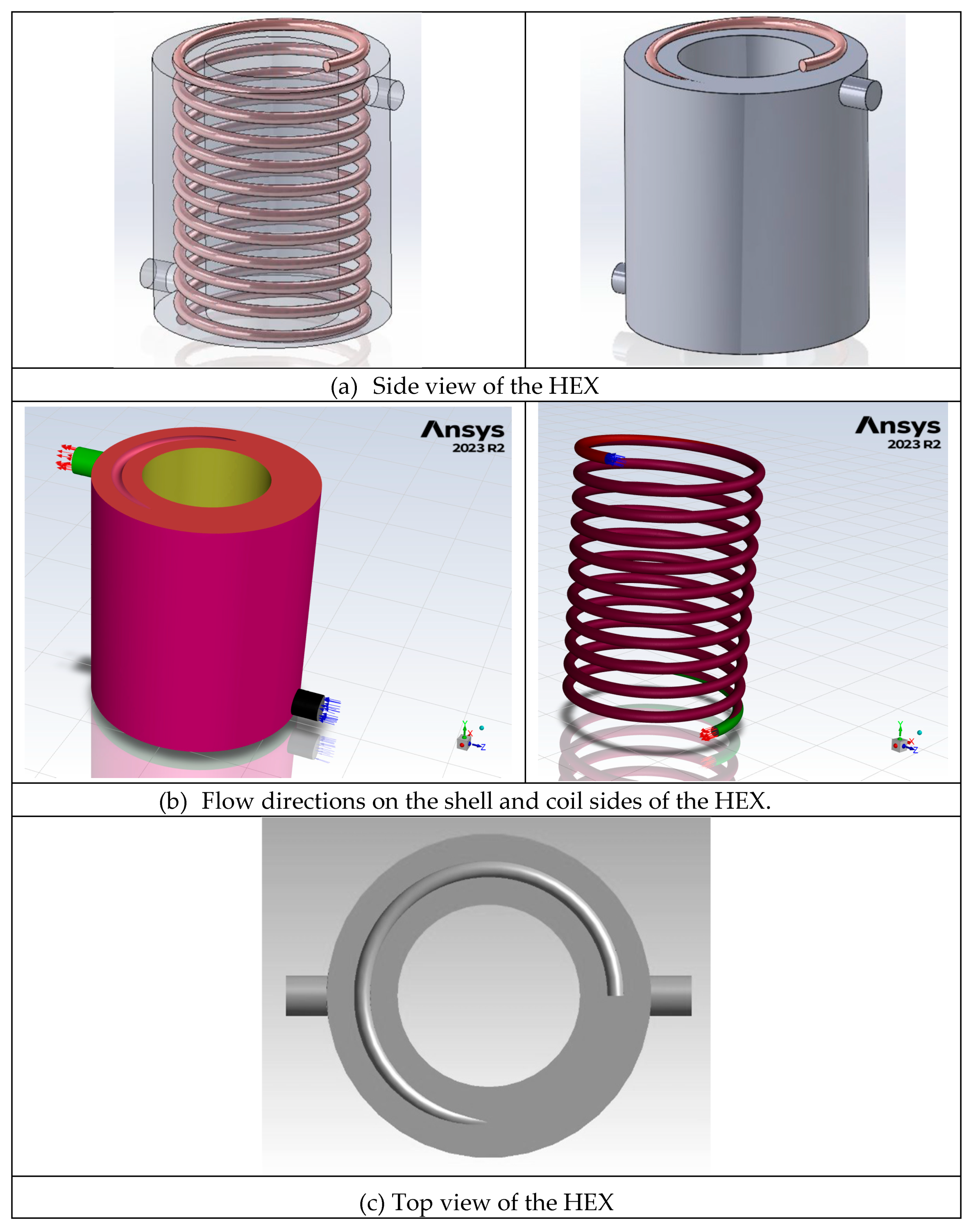
Figure 2.
The shaded surface represents the cross-section area of the shell side of the HEX that is available for the fluid flow.
Figure 2.
The shaded surface represents the cross-section area of the shell side of the HEX that is available for the fluid flow.

Figure 3.
Representative meshing strategy for the HCTHEX. The computational domain was discretized using a hybrid poly-hexacore mesh composed of hexahedral and poly-prism elements to ensure accuracy in both the axial and cross-sectional directions.
Figure 3.
Representative meshing strategy for the HCTHEX. The computational domain was discretized using a hybrid poly-hexacore mesh composed of hexahedral and poly-prism elements to ensure accuracy in both the axial and cross-sectional directions.
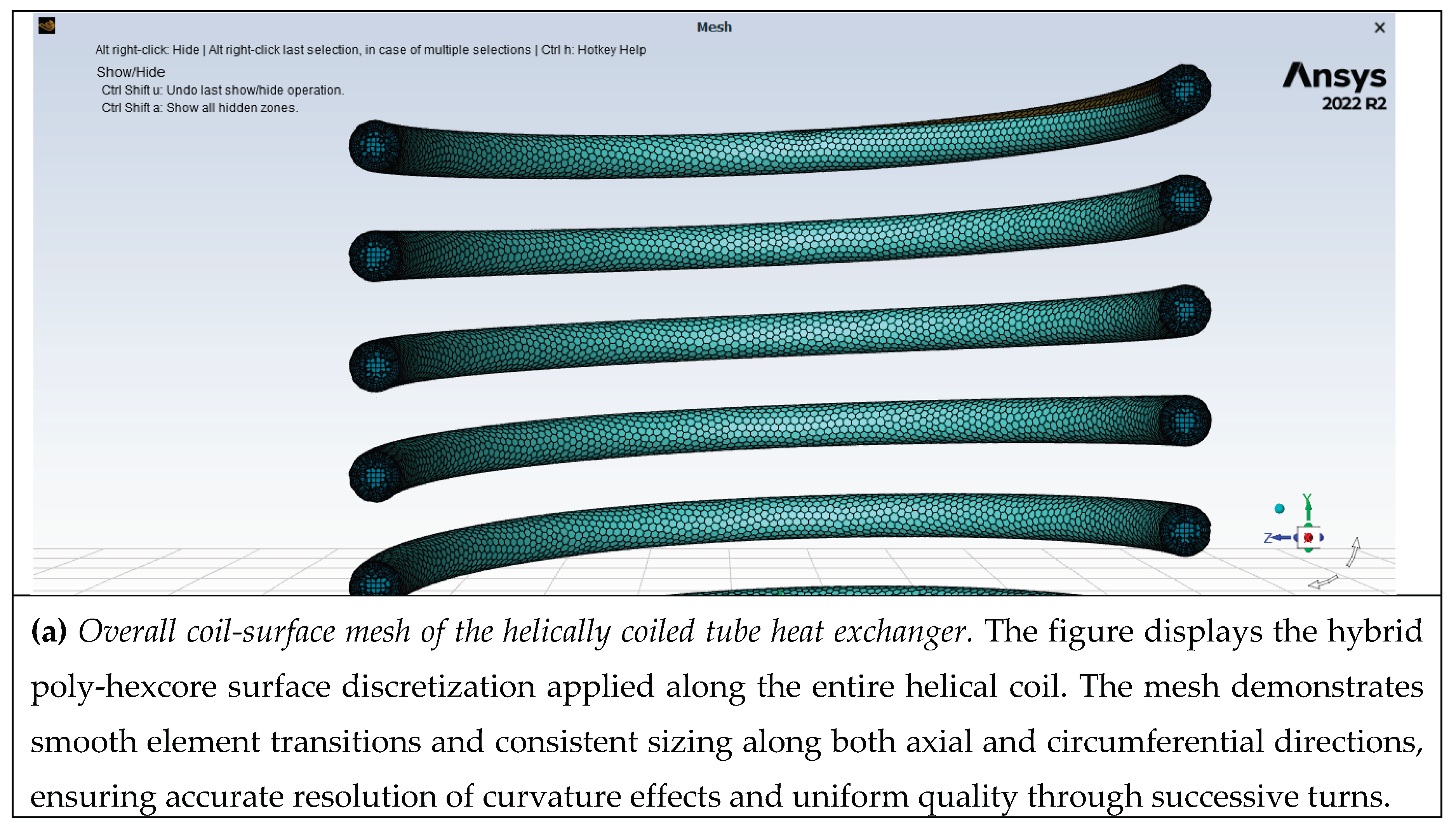
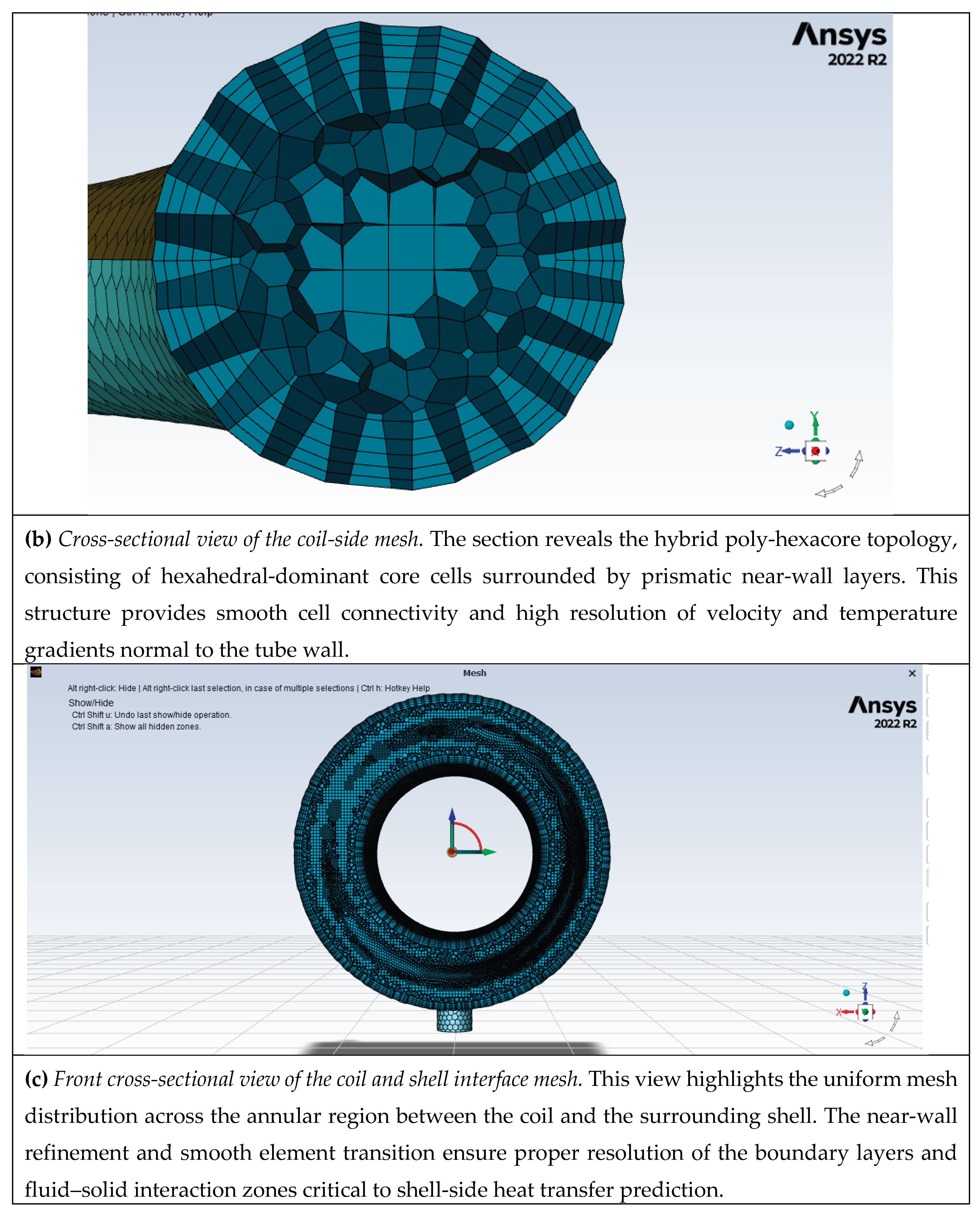
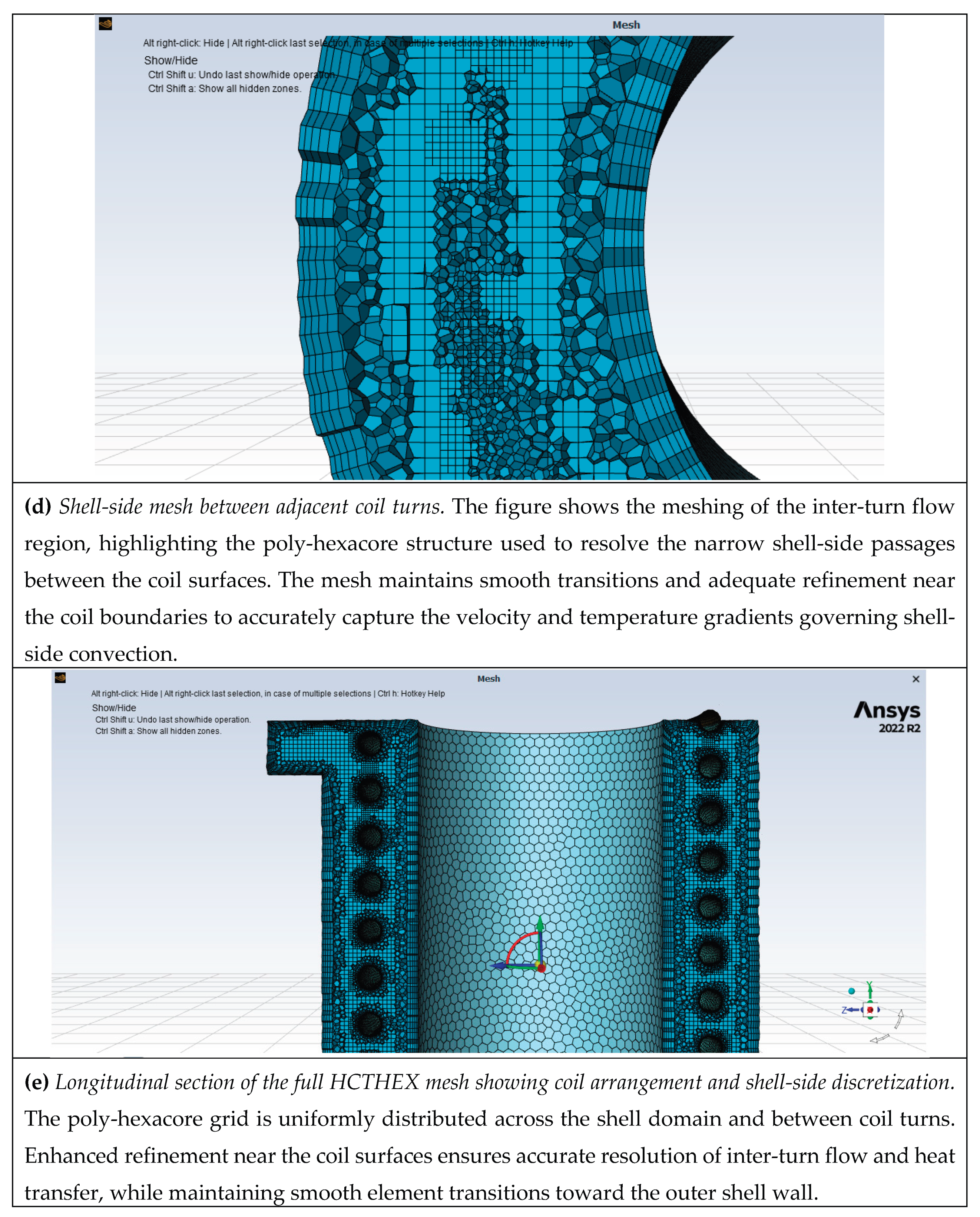
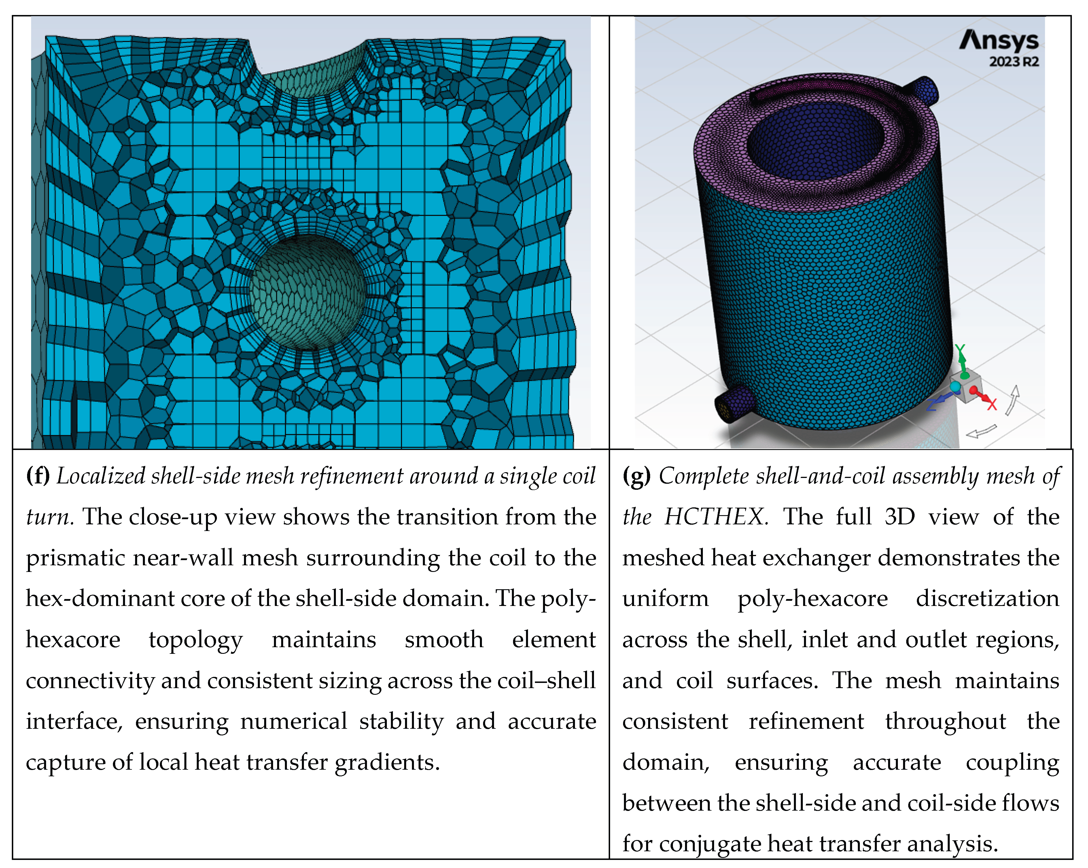
Figure 4.
Variation of shell-side Nusselt number () with shell-side Reynolds number () for the helically coiled tube heat-exchanger dataset.
Figure 4.
Variation of shell-side Nusselt number () with shell-side Reynolds number () for the helically coiled tube heat-exchanger dataset.
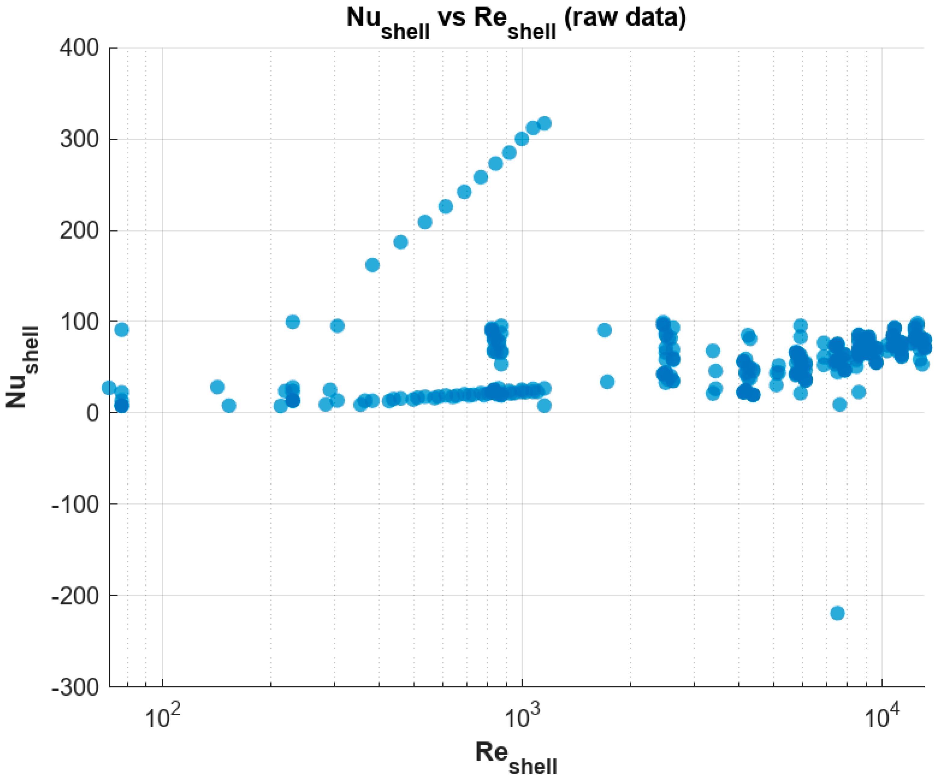
Figure 5.
Parity plot illustrating the predicted vs. Actual Nusselt Number using a) Power-Law, b) Log-Quadratic, c) GAM/Ensemble Model. The dashed red line denotes the perfect 1:1 correlation, confirming the predictive reliability of the GAM/Ensemble-based Nusselt number correlation.
Figure 5.
Parity plot illustrating the predicted vs. Actual Nusselt Number using a) Power-Law, b) Log-Quadratic, c) GAM/Ensemble Model. The dashed red line denotes the perfect 1:1 correlation, confirming the predictive reliability of the GAM/Ensemble-based Nusselt number correlation.
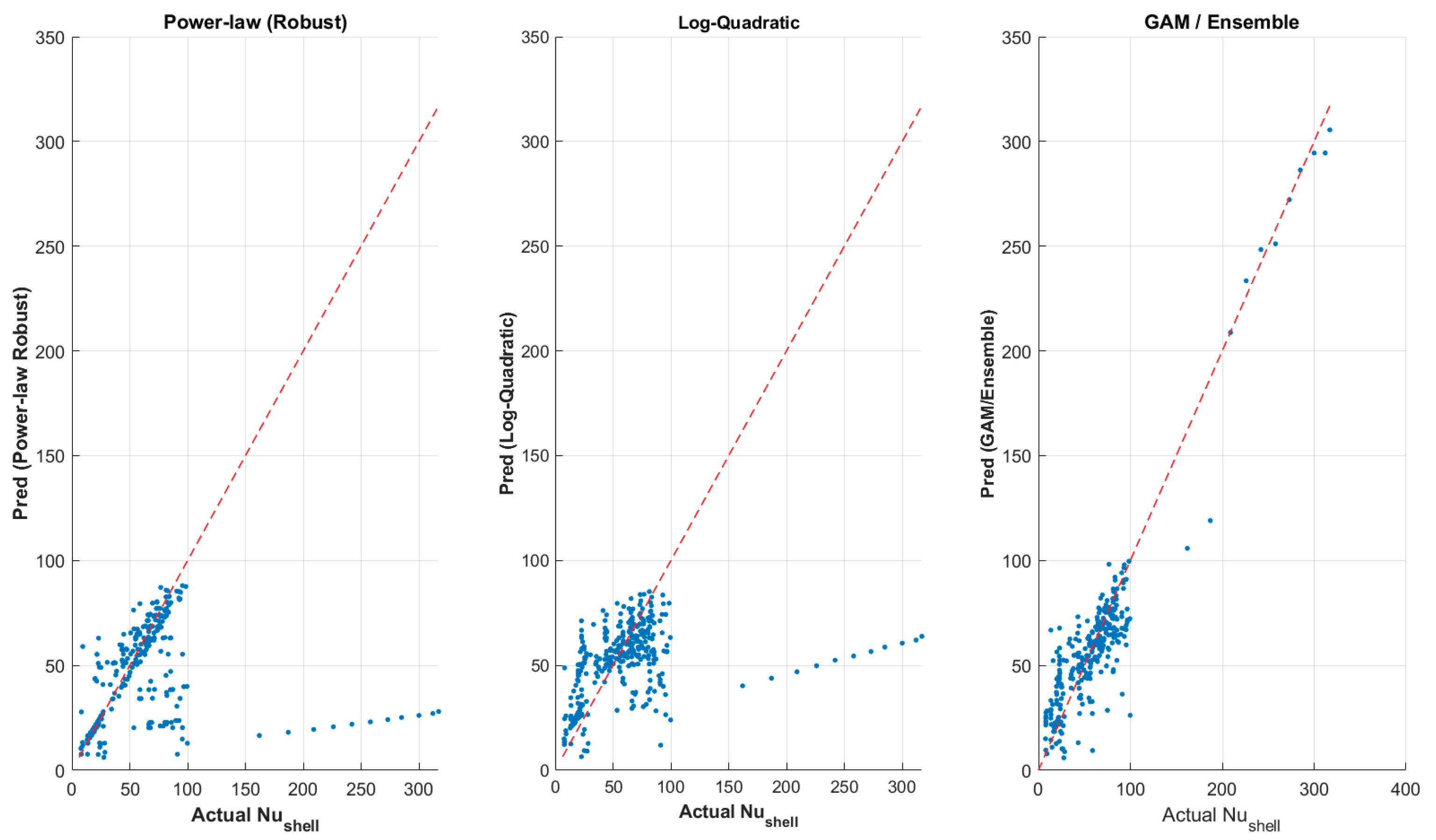
Table 1.
Coils and shell specifications.
|
|
|
|
|
|
|
|
||
|---|---|---|---|---|---|---|---|---|
| 160 | 90 | 9.52/8.001 | 125 | 1.8 | 10.50 | 180 | 1.03771e+05 | 11.57 |
| 160 | 90 | 9.52/8.001 | 125 | 1.85 | 10.22 | 180 | 1.00974e+05 | 11.84 |
| 160 | 90 | 9.52/8.001 | 125 | 1.90 | 9.95 | 180 | 9.83241e+04 | 12.10 |
| 160 | 90 | 9.52/8.001 | 125 | 1.95 | 9.70 | 180 | 9.58106e+04 | 12.35 |
| 160 | 90 | 9.52/8.001 | 125 | 2 | 9.45 | 180 | 9.34230e+04 | 12.60 |
| 160 | 90 | 12.5/10.98 | 125 | 1.8 | 7.11 | 360 | 0.92330e+05 | 0.010.17 |
| 160 | 90 | 12.5/10.98 | 125 | 1.9 | 6.74 | 360 | 0.87494e+05 | 10.74 |
| 160 | 90 | 12.5/10.98 | 125 | 2 | 6.40 | 360 | 0.83142e+05 | 11.27 |
Table 2.
Comparison of the coil-side Nusselt number and equation (7).
| Dimensionless pitch | Discrepancies |
| 1.8 | 7.05% |
| 1.85 | 4.98% |
| 1.9 | 8.74% |
| 1.95 | 0.7% |
| 2 | 4.42% |
Table 5.
Summary of different models’ accuracies.
| Model | R² | RMSE |
| Power-law (OLS) | −0.0076 | 44.94 |
| Power-law (Robust) | −0.1368 | 47.73 |
| Log-Quadratic | 0.1003 | 42.47 |
| GAM/Ensemble (True Model) | 0.8279 | 19.60 |
| Polynomial-in-log Approximation | −0.0240 | 47.82 |
Table 3.
Numerically simulated versus equation (7) comparison.
| Dimensionless pitch | Discrepancies |
| 1.8 | 7.7% |
| 1.85 | 9.1% |
| 1.9 | 5.3% |
| 1.95 | 3.7% |
| 2 | 4.4% |
Disclaimer/Publisher’s Note: The statements, opinions and data contained in all publications are solely those of the individual author(s) and contributor(s) and not of MDPI and/or the editor(s). MDPI and/or the editor(s) disclaim responsibility for any injury to people or property resulting from any ideas, methods, instructions or products referred to in the content. |
© 2025 by the authors. Licensee MDPI, Basel, Switzerland. This article is an open access article distributed under the terms and conditions of the Creative Commons Attribution (CC BY) license (http://creativecommons.org/licenses/by/4.0/).
Copyright: This open access article is published under a Creative Commons CC BY 4.0 license, which permit the free download, distribution, and reuse, provided that the author and preprint are cited in any reuse.


