
Submitted:
24 July 2025
Posted:
25 July 2025
You are already at the latest version
Abstract
The helical-coiled tube (HCT) heat exchanger (HX) has been applied in the nuclear industry, especially HXs in the residual heat removal system for nuclear power plants (NPPs) and steam generators for small modular reactors. In this paper, a single-phase CFD model is developed to investigate the non-uniform circumferential distributions in the wall heat transfer characteristics for a vertically HCT since the localized information is needed for the safety of NPPs. As shown in comparison, predicted circumferential heat transfer characteristics agree well with data. Governed by the centrifugal/gravitational forces, these non-uniform distributions can be clearly seen in the present results, enhancing explanation of test data. Additional simulations are also performed using the conjugated heat transfer from the hot fluid of shell side to the cold fluid of tube side, confirming that the inhomogeneity of circumferential distributions for a HCT is essentially caused by assumption of constant-heat-flux boundary condition.
Keywords:
helical-coiled tube
; inhomogeneity of circumferential wall temperature
; CFD modelling
; centrifugal and gravitational forces
1. Introduction
Due to the special shape of curvature, a helical-coiled tube (HCT) can withstand the greater thermal expansion stress as the spring, as well as have the larger heat exchange area within the given volume and the higher heat transfer capability due to the stronger secondary flow caused by the centrifugal force. Then, the HCTs have been extensively applied in the industry components, especially for the heat exchanger. In the nuclear power plants (NPPs), the HCT heat exchanger (HCTHX) is designed in the Residual Heat Removal System (RHRS) and the Steam Generator (SG) for the Small Modular Reactors (SMRs). Most of previous works for the HCT heat exchanger (HCTHX) are focused on its overall heat transfer capability and performance. However, the localized information (like hot spot or inferior heat transfer point) is needed for the operational safety of NPPs. In this work, the CFD simulations have been performed to investigate the localized heat transfer characteristics of single-phase convection in a HCT, which can be considered as an assistance tool for the nuclear safety in the operation and maintenance.
Numerical works related to the single-phase convective heat transfer for a HCTHX had been reviewed. Ferng et al. [1] developed a 3-D single-phase CFD model to investigate effects of Dean (De) number and pitch size on the thermal-hydraulic characteristics in a HCTHX. The average Nussel (Nu) number versus the tube length had been presented and compared with the measured data and appropriate correlations. Based on their simulation results, the overall phenomena in the HCTHX had be reasonably captured, which included the flow acceleration and separation in the shell side, the secondary flow within the tube, and the developing behaviors near the entrance of coiled tube, etc. Through the single-phase numerical simulations, Lin et al. [2] investigated the effects of different turbulence models on the flow and heat transfer characteristics in a HCTHX. Three turbulence models were considered, including the realizable k–ε turbulence model (RKE), low-Reynolds k–ε turbulence model (LKE), and Reynolds stress model (RSM). They reported that the LKE turbulence model would over-predicted the heat exchanger performance as compared with the other two models and measured data. Alimoradi and Veysi [3] numerically and experimentally studied the heat transfer of HCTHX under various parameters, including the physical properties of fluid, operational parameters, and geometrical parameters. Their results showed that the shell side Nu number increased with the increasing pitch and decreased with the increasing height and diameter of the shell. In addition, two correlations were developed to predict Nu numbers of coil side and shell side for wide ranges of Reynolds (Re) and Prandtl (Pr) numbers. In the work of Sepehr et al. [4], the heat transfer, pressure drop and the entropy generation in shell and helically coiled finned tube heat exchanger was numerically studied. Effects of the fins height and number were considered. Their model was validated by comparing the overall Nu of both side and average friction factor of the coil side with the appropriate empirical correlations.
Elattara et al [5] numerically investigated the thermal and hydraulic performance of the MTTHC (Multi-Tubes in Tube Helically Coiled) for the turbulent flow. Effects of the operating and geometrical parameters of the coil on the Nu number, pumping power, and effectiveness etc., were also considered. Their results showed the largest heat transfer coefficient and effectiveness were predicted at inner tube = 3 and coil inclination angle = 0° & 90°. Mirgolbabaei [6] performed the thermal performance assessment of vertical HCTHX at various mass flow rates, coil-to-tube diameter ratio, and coil pitch. A conjugate thermal boundary condition for the tube wall fluid-to-fluid heat transfer mechanism, was considered. Based on the simulation results, the effectiveness of heat exchanger decreased with increasing coil pitch and had not been influenced by varying the tube diameter. Using single-phase CFD approach, Tuncer et al. [7] compared the performance of modified shell and helically coiled heat exchanger (SHCHX) with a conventional one. This modified SHCHX was designed with a hollow tube integrated into the shell side with advantage of regulating the fluid flow in the shell side and improving the heat transfer. The corresponding modified SHCHX had been experimentally tested to determine its effectiveness. They reported that average difference between predicted and measured results was 8%.
Güngor et al. [8] attached the rings and discs to the helical-coiled tubes to modify the conventional HCTHX. According to their simulation results, average heat transfer rate for the modified the heat transfer rate increased to 7.1 % as compared to the conventional one. In addition, the modified HX was fabricated and was experimentally tested with same conditions in laboratory to verify the simulation results. The comparison results revealed that the simulation results were close to the experimental data with difference of 2.4 % in terms of average heat transfer rate. Xu et al. [9] performed the numerical simulations to study the effects of various grooving methods and depths on the overall heat transfer characteristics of HCTHXs. Their results implied that grooving on the plain tube could enhance the comprehensive heat transfer performance and simultaneously increase the pressure drop of the fluid. They concluded that the maximum performance evaluation criterion (PEC) was occurred for the helical-coiled spiral grooved tube (HCSGT) HXs with 0.5 mm groove depth. Yuan et al. [10] numerically and experimentally study the performance of the double shell-passes multi-layer helical-coiled tubes heat exchanger (DSMHCTHX). Both results confirmed that the heat transfer rate and thermal effectiveness of DSMHCTHX increased by 5.1 % to 12.9 %, compared with the traditional multi-layer helical tube heat exchanger. However, the shell-side pressure drop increased by 60.7 % to 83.4 %.
Duan et al. [11] developed a tube-shell coupled model for the helical-coiled corrugated tube heat exchanger. The effects of Re number, corrugation height, and corrugation length on flow and heat transfer performance were also considered. They concluded that the Nu number for both sides, and PEC significantly increased with the increasing corrugation height and the decreasing length. However, the corrugation height would enhance the friction factor, but its length had a little impact. Cao et al. [12] numerically studied the heat transfer and flow resistance characteristics for the internally finned helical-coiled tubes heat exchanger. The corresponding tests were also performed. The empirical correlations to calculate the Nu number and friction factor of internally finned helicall-coiled tubes were summarized and validated using the measurements and predictions. They also reported that the internally finned helical-coiled tubes heat exchangers had better performance than smooth HCTHXs. Through CFD simulations, Missaoui [13] investigated the influence of different helical coil structure designs on its heat transfer characteristics, including constant-diameter coil, variable-diameter coil and variable-pitch coil. This CFD model had been validated with the experimental measurements. They reported that the values of Nu number for the helical coil with variable pitch were higher than those of other configurations.
As the aforementioned literature review, most of CFD works related to the HCT or HCTHXs are focused on the overall heat transfer behavior and their performance. Seldom CFD simulations are conducted to study the localized heat transfer characteristics. However, the localized information just put the challenge to the safety of NPPs. Developing the single-phase CFD model based on the Best Practice Guidelines (BPGs) [14], the preset simulation work can capture the localized heat transfer characteristics in a HCT. This CFD methodology has been validated with the test data of the non-uniform circumferential distributions of wall temperature and heat transfer coefficient [15]. Combined with the experimental results, the present model can assess the applicability of correlations suitable for the heat transfer in a HCT tube. In addition, the simulation results from this CFD model can help explain the measured results using the predicted thermal-hydraulic contours on the cross-section of HCT, which can also assist in analyzing the design and operation safety of HCTHXs for the NPPs.
2. Mathematical Model and Numerical Treatment
A 3-D CFD methodology is developed in this paper to simulate the non-uniform circumferential distributions of single-phase heat transfer characteristics in a HCT. The RANS equations with the SST k-ω turbulence model (SSTKW) [16] are adopted since the SSTKW can have better prediction for the flow conditions of adverse pressure gradients, swirling pattern, and secondary flow due to the centrifugal and gravitational forces in a HCT. The mathematical model can be described as follows:
2.1. Governing Equations
Continuity Equation
Momentum Equation
where,;
Energy Equation
where,
2.2. SST Turbulence Model
The turbulence kinetic energy (k) and the specific dissipation rate (ω) in the SSTKW can be obtained from the following transport equations.
where,
is the mean rate-of-rotation tensor and is defined by
The blending functions, F1 and F2, are given by
is the positive portion of the cross diffusion term and is determined by
The value of empirical constants shown above are illustrated in Table 1.
2.3. Numerical Treatment
The mathematical model described in the previous section belongs to the partial differential equations (PDEs). Using the finite difference or finite volume method, these PDEs should be discretized into the algebraic equations for the numerical calculation. The second-order upwind scheme is adopted to treat the convection terms in these PDEs. The SIMPLE scheme [17] is used to solve the equations for velocities coupled with pressure. The Algebraic MultiGrid (AMG) linear solver is adopted for all the equations. All of the simulation works presented in this paper was performed using the FLUENT code [18] on the PC with Intel® Core i9-7900X cpu and the calculation for the typical case needs approximately 2 hrs computing time. The convergence criteria for all of the governing equations are set such that the summation of the relative residual in every control volume is less than. In addition, the decay trend in the residual plot for each equation is also considered as an alternative criterion. Both of these criteria should be met to ensure the convergence of the numerical simulations.
3. Results and Discussion
The experimental work [15] for measuring the non-uniform circumferential distributions of wall temperature and heat transfer coefficient for a HCT is adopted to assess the present CFD methodology. Figure 1 shows the schematics of HCT for the present simulations. The right portion of this figure represents the circumferential angle (φ) on the HCT wall. The corresponding mesh distributions on the cross-section of HCT are indicated in Figure 2. Based on the requirements of the CFD Best Practice Guidelines [14], the structured grids should be adopted near the wall and mesh independent calculations should be performed. The sensitivity simulations for the various mesh are applied on the cross-section of HCT, including 860 (Coarse), 1,425 (Standard), and 3525 (Fine) cells, respectively. The corresponding values of y+ for these three mesh models are 28.9~36.2 (Coarse), 0.8~1.2 (Standard), and 0.6~1.1 (Fine). Uniform girds are adopted along the HCT with the interval of 10o helical coil. The constant heat flux is set at the tube wall; the inlet mass flux and temperature are set at the tube inlet; the pressure is set at the tube outlet. The simulation conditions for all the case are listed in Table 2. Figure 3 compares the predicted results for the circumferential distributions of wall temperature at x = -0.147 under the coarse, standard, and fine mesh. The conditions of Case 1 in Table 2 and the SSTKW turbulence model are adopted. In this figure, the abscissa represents the circumferential angle (φ) of HCT. Similar to the location index using the quality (x) in the measured data presentation of Wang et al., [15], x is also adopted as the location index of HCT. As illustrated in the upper portion of Figure 3, φ = 90o and 270o are the tube wall on the outer and inner sides, respectively, of HCT. This figure implies that the predicted result of circumferential temperature distribution using the standard mesh is close to that from the fine mesh.
Since the BPGs provides useful guidelines for the single-phase applications of CFD to nuclear reactor safety (NRS) problems [14], these guidelines should be followed to ensure accuracy and credibility of CFD predictions. The essential requirements for the BPGs are applied in the mesh model, the physical models, especially the turbulence model, and the model validation. Therefore, in addition to the mesh model, the sensitivity calculations of turbulence models are also conducted, including the SKE, RKE, and SSTKW. The blind calculations using different turbulence models are clearly revealed in Figure 4 and the simulation conditions are the same as those in Figure 3. As shown in this figure, the predicted results of circumferential wall-temperature distribution at x = -0.147 using both the SSTKW and the RKE are similar. Both the SSTKW and RKE turbulence models provide superior performance for flow characteristics with adverse pressure gradient, recirculation, and separation, which are similar to the flow characteristics in a HCT. The SSTKW is less sensitive to the inlet turbulence properties and less restriction for the near-wall mesh model. Therefore, the SSTKW turbulence model and the standard mesh are adopted to be assessed in the followings (Figure 5, Figure 6 and Figure 7) with the experimental data and then applied in the extended discussion in the thermal-hydraulic characteristics in a HCT with confidence.
Figure 5 compares the circumferential distributions of wall temperature at x = -0.147 (L = 2.07 m) and -0.236 (L = 0.57 m), respectively, predicted by the present CFD model (red dots) with those from the measurements (blue dots) for Case 1. It can be clearly seen in this figure that the predicted distributions agree well with the measured ones at these two locations. Both the measured and predicted results also show the strong non-uniform circumferential distribution of wall temperature for the HCT. As the aforementioned descriptions, the thermal-hydraulic characteristics in a HCT are governed by the centrifugal force and the gravitational force. The lower-temperature water with the higher density would be push to the outer portion of HCT due to the centrifugal force and tends to accumulate on the lower portion of tube due to the gravitational force. As shown in Figure 6 (a), the higher-density water is located near the outer and right-bottom portion of HCT (φ ~ 135 o). In addition, the lower density water with the higher-temperature water can be found near φ = 315o. These predicted density distributions can provide the obvious images to explain the inhomogeneity distribution of circumferential wall temperature, which cannot be revealed in the measured results.
As the mass flux in the HCT decreases (i.e. Case 2), the thermal-hydraulic characteristics are governed by the gravitational force more than the centrifugal force. The lower-temperature water with the higher density is accumulated in the lower portion of HCT than that for the Case 1. This difference can be found in the density contours for both cases, as clearly revealed in the comparison of Figures 6 (a) and (b). Figure 7 (a) shows the circumferential distributions of wall temperature at x = -0.167 (L = 1.49 m) and -0.219 (L = 0.74 m), respectively, obtained from the CFD simulations (red dots) and the test data (blue dots) for Case 2. As revealed in this figure, the lower wall temperature is located near φ = 180o and the higher wall temperature appears near φ = 360o. Both the measured and predicted results show this trend. In contrast to the Case 2 with the lower mass flux, the inlet mass flux increases enough (i.e. Case 3) so that the gravitational effect can be neglected as shown in Figure 7 (b) that is the circumferential distributions of wall temperature at x = -0.108 (L = 4.76 m) and -0.197 (L=2.15 m), respectively, for Case 3. Therefore, The peak wall temperature then is predicted to occur at φ = 270o. The thermal-hydraulic characteristics for Case 3 are symmetric along the horizontal line on the cross-section for a vertical HCT, as clearly shown in the density contour of Figure 6 (c). In addition, the predicted values for the circumferential distributions of wall temperature also correspond well with the measured ones, as clearly seen in both plots of Figure 7.
The Lu number represents the ratio of centrifugal force and buoyancy and can be written as
This non-dimensional number can characterize the flow and heat transfer patterns for the HCT. The Lu number increases with the increasing mass flux in a HCT, which also enhances the influence of centrifugal force, and vice versa. Therefore, three simulation cases with the Lu number of 1.226, 0.12, and 13.7 are selected in the present work, which characterizes the middle (centrifugal force balanced by buoyancy force), low (buoyancy force dominated), and high (centrifugal force dominated) Lu number, respectively. Figures 8 (a) and 9 (a) show the distribution patterns of temperature on the cross-section of HCT for Case 1 and Case 2. Combined observation of density and temperature contours in Figure 6 (a) and Figure 8 (a) reveals that the higher heat transfer region with the lower-density and higher-temperature water is located near the upper left corner and the lower heat transfer one with the higher-density and lower-temperature water is near the lower-right corner. These predicted results can provided the clear images of two-region flow and heat transfer characteristics. This two-region heat transfer pattern is also confirmed in the experimental work of Wang et al. [15]. They suggested the schematic of two-region heat transfer patterns with the higher heat transfer region in the upper-left corner and the lower heat transfer one in the lower-right corner, as indicated in Figure 8 (b). The predicted heat transfer flow pattern from the present CFD results and the schematic one from the work [15] for Case 2 are also revealed in Figures 9 (a) and (b) , respectively.
The vector distributions of secondary flow on the cross-section of HCT are also plotted on Figures 8 (a) and 9 (a). As clearly shown in these plots, a vortex-pair of secondary flow is shown on these cross-sections of HCT and the higher wall temperature occurs where the secondary flow leaves away. In addition, Figure 8 (a) indicates that the higher wall temperature may appear between φ =270o and 315o. However, the circumferential distribution of measured temperatures is presented in the discrete pattern on the selected locations only. Based on the measured data of Case 1, the peak wall temperature at x = -0.147 occurs at φ = 270o. However, as shown in Figure 8 (c), the peak wall temperature is located at φ ~ 308o. The exact location of peak wall temperature can be captured only in the CFD results and cannot be revealed in the experimental data, which is one of the main contributions for the CFD simulations. Similar result for Case 2 is also shown in Figure 9 (c). The peak wall temperature at x = -0.167 is measured at φ = 0o (i.e. 360o), while the peak wall temperature may be actually at φ ~ 342o, based on the predicted result. Therefore, in addition to matching the measured data, the calculated results from the present CFD model then can help interpret the test results and expand their application.
Figure 10 compares the circumferentially averaged heat transfer coefficients in different regions, which are obtained from the measurements and the predictions for Case 2 and Case 3, respectively. As shown in Figure 10 (a) of Case 2 with Lu < 0.25, two regions with the different averaged heat transfer along the HCT circumferential wall is suggested from the work [15], including φ = 270o - 45o (i.e regions A, B, G, H) and 90o -225o (i.e. regions C, D, E, F). The definition of A-H regions is illustrated in the right portion of this plot. The former region (i.e regions A, B, G, H) is the lower heat transfer region where the higher temperature water with the lower density occurs and the latter region is the higher heat transfer one. It can be clearly revealed in Figure 10 (a) that the circumferentially averaged heat transfer coefficients over the regions A, B, G, H, the regions C, D, E, F, and the overall circumferential wall (i.e. defined Avg. in the Figure 10 (a)) predicted by the present CFD model correspond well with those from the experiment. The non-uniform distribution for the wall heat transfer coefficients can be also shown in both the measurements and predictions.
The quantity correspondence between the measured and predicted heat transfer coefficient at the different regions as well as its average value is also shown in Figure 10 (b) for Case 3. Three regions with different heat transfer characteristics are only suggested based on the measured data, but these characteristics have been clearly seen in the present predicted results in the density contour of Figure 6 (c). In addition, the predicted heat transfer coefficients shown in plots (a) and (b) of Figure 10 are the fully-developed one. The heat transfer coefficient would decrease from the inlet of HCT and approaches to the fully-developed value, as clearly revealed in Figure 10 (c) for Case 3. In this plot, the longitudinal axis is the normalized heat transfer coefficient (hnorm) that is the local h divided by the fully-developed one. The abscissa axis is the distance from the inlet of HCT. Detailed observation of this plot implies that the entrance length (developing length) is about 42 ~ 50 pipe diameter (d). The correlation for the entrance length for a HCT has been proposed by Saffari et al. [19]) and is expressed as the function of Reynolds number (Re), Dean number (De), and curvature ration (δ).
Using the conditions of Case 3, the entrance length calculated using this correlation is 51.24 that is close to the present predicted range.
In addition, the thermal-hydraulic characteristic would reach the fully-developed condition as the flow passes over the coil angle (ψ) of 210o ~ 275o based on the coil/tube diameter values, implying that the entrance effect may be neglected for evaluating the overall heat transfer characteristics for a whole HCT or HCTHX. Then, the fully-developed correlations of heat transfer coefficient can be applied to estimate the heat transfer capability for a HCT or HCTHX. Figure 11 compares the fully-developed heat transfer coefficient for a HCT obtained from the present CFD model, the appropriate correlations, and experiment for Case 2 (a) and Case 3 (b). These correlations include those proposed by Rogers and Mayhew [20], Mikaila & Poskas [21], Xin & Ebadian [22], Guo et al. [23], Hardik et al. [24], and El-Genk & Schriener [25] since Gou et al. [23] had suggested that these correlations are suitable for predicting the heat transfer coefficient for a HCT. Similar to the comparison in Figure 10, the agreement between the predicted h and the measured one is also shown in this figure under different flow conditions. In addition, the calculated h from the Xin & Ebadian’s correlation [22] matches with the data better than that from others for Case 2 and the h calculated using the correlation of Rogers & Mayhew [20] or Mikaila & Poskas [21] shows more agreement with the data for Case 3. Therefore, these comparison results strong imply that applicability of various kinds of h-correlation for the HCTs depends on their flow conditions, which reveals that the contribution of CFD simulation in this area.
The inhomogeneity of circumferential distributions for single-phase heat transfer characteristics for a vertically helical-coiled tube are clearly shown in Figure 5, Figure 6, Figure 7, Figure 8, Figure 9 and Figure 10, which is essentially caused by the constant-heat-flux boundary condition. This boundary condition for CFD simulations is not suitable to investigate the flow and heat transfer behaviors within the HCTHX, as described in the work of Bahrehmand and Abbassi [26]. The higher wall temperature occurs near the region with inferior heat transfer under the condition of constant. However, the heat transfer mechanism for a HCT heat exchange is mainly belong to the conjugated heat transfer from the hot fluid in the shell side to the cold fluid in the tube side. The wall heat flux would decrease around the location with the poor heat transfer capability within the tube side, suppressing this higher-wall-temperature phenomenon. Therefore, the conjugated heat transfer effect by including the shell-side solution domain is simulated herein in order to investigate the effect of conjugated heat transfer on the non-uniform characteristics of HCT wall in the HCTHX. Figure 12 compares the circumferential dependence of normalized temperature predicted using the constant-heat flux BC and the conjugated heat transfer simulation, respectively. The normalized temperature shown on the longitudinal axis is the local wall temperature divided by the average wall temperature. The simulation conditions under the constant-heat-flux cases in Figures 12 (a) and (b) are similar to those for Cases 1 and 3. The inlet mass flux/temperature and pressure of tube side for the conjugated-heat-transfer cases are the same as those for the constant-heat-flux ones. For the conjugated-heat-transfer cases, the mass flowrate in the shell side is set to be 0.2 kg/s. The temperature drops for the shell side in Figures 12 (a) and (b) are set to be 35.6 and 58.1 oC, respectively, so that the heat transfer rate from the shell side to the tube is similar to that set in the constant-heat-flux cases. It can be clearly shown in Figure 12 that the non-uniform circumferential distribution of heat transfer is essentially caused by the constant-heat-flux boundary condition on the HCT wall. This characteristic can be significantly reduced by actually considering the heat transfer from the shell side.
4. Conclusions
In this study, the CFD methodology is developed to predict the non-uniform circumferential distributions of heat transfer characteristics for a single-phase convection in a HCT. The effects of inlet mass fluxes on this inhomogeneity of a HCT are also considered. The present CFD model is validated with the experiments of Wang et al. [15] using the circumferential distributions of wall temperature and heat transfer coefficient under various inlet mass fluxes. The values and locations of peak wall temperature predicted by the present model correspond well with the measured ones. The inhomogeneity of flow and heat transfer for a HCT are essentially caused by both the centrifugal and gravitational forces, which depends on the inlet mass fluxes. These non-uniform characteristics can be clearly explained using the predicted density and temperature contours, and secondary flow vectors on the cross-section of HCT. These calculated results can provide the detailed visualization of thermal-hydraulic characteristics within a HCT, which is seldom captured in the measured results. This is one of the main contributions of CFD simulations. In addition, additional simulations are also performed using the conjugated heat transfer from the hot fluid in the shell side to the cold fluid in the tube side. Compared with the simplified constant-heat-flux BC, this conjugated heat transfer is the actual heat transfer phenomenon for a HCTHX. The comparison results clearly show that the inhomogeneity of circumferential distributions for the single-phase heat transfer characteristics of a HCT is essentially caused by the assumption of constant-heat-flux BC. These characteristics can be suppressed by considering the conjugated-heat-transfer, which is the actual heat transfer condition for a HCTHX.
Acknowledgments
This work was supported by National Science and Technology Council of Taiwan under NSTC 113-2221- E-007-123.
Nomenclature
| Cp | specific heat capacity, J/kg-K |
| h | heat transfer coefficient, W/m2-K |
| average enthalpy on the cross-section of HCT, J/kg | |
| hf | saturated liquid enthalpy, J/kg |
| hfg | latent heat, J/kg |
| L | distance from HCT inlet, m |
| p | pressure, N/m2 |
| heat flux, W/m2 | |
| T | temperature, K |
| u | velocity, m/s |
| x | |
| xi | coordinate, m |
| y+ | non-dimensional wall distance |
| Greek symbols | |
| thermal conductivity, W/m-K | |
| density, kg/m3 | |
| μ | viscosity, N-s/m2 |
| τ | shear shress, N/m2 |
| φ | circumferential angle, o |
| Subscripts | |
| i,j | tensor index |
References
- Ferng, Y.M.; Lin, W.C.; Chieng, C.C. Numerically investigated effects of different Dean number and pitch size on flow and heat transfer characteristics in a helically coil-tube heat exchanger. Appl. Therm. Eng. 2012, 36, 378–385. [Google Scholar] [CrossRef]
- Lin, W.C.; Ferng, Y.M.; Chieng, C.C. Numerical computations on flow and heat transfer characteristics of a helically coiled heat exchanger using different turbulence models. Nucl. Eng. Des. 2013, 263, 77–86. [Google Scholar] [CrossRef]
- Alimoradi, A.; Veysi, F. Prediction of heat transfer coefficients of shell and coiled tube heat exchangers using numerical method and experimental validation. Int. J. Therm. Sci. 2016, 107, 196–208. [Google Scholar] [CrossRef]
- Sepehr, M.; Hashemi, S.S.; Rahjoo, M.; Farhangmehr, V.; Alimoradi, A. Prediction of heat transfer, pressure drop and entropy generation in shell and helically coiled finned tube heat exchangers. Chem. Eng. Res. Des. 134, 277–291. [CrossRef]
- Elattara, H.F.; Foudab, A.; Nadaa, S.A.; Refaeyc, H.A.; Al-Zahranid, A. Thermal and hydraulic numerical study for a novel multi tubes in tube helically coiled heat exchangers: Effects of operating/geometric parameters. Int. J. Therm. Sci. 2018, 128, 70–83. [Google Scholar] [CrossRef]
- Mirgolbabaei, H. Numerical investigation of vertical helically coiled tube heat exchangers. Appl. Therm. Eng. 2018, 136, 252–259. [Google Scholar] [CrossRef]
- Tuncer, A.D.; Sozen, A.; Khanlari, A.; Gürbüz, E.Y.; Variyenli, H.I. Analysis of thermal performance of an improved shell and helically coiled heat exchanger. Appl. Therm. Eng. 2021, 184, 116272. [Google Scholar] [CrossRef]
- Güngor, A.; Khanlari, A.; Sozen, A.; Variyenli, H.I. Numerical and experimental study on thermal performance of a novel shell and helically coiled tube heat exchanger design with integrated rings and discs. Int. J. Therm. Sci. 2022, 182, 107781. [Google Scholar] [CrossRef]
- Xu, P.; Zhou, T.; Xing, J.X.; Chen, J.; Fu, Z.G. Numerical investigation of heat-transfer enhancement in helically coiled spiral grooved tube heat exchanger. Prog. Nucl. Energy 2022, 145, 104132. [Google Scholar] [CrossRef]
- Yuan, Y.Y.; Cao, J.M.; Zhang, Z.; Xiao, Z.Y.; Wang, X.S. Experimental and numerical simulation study of a novel double shell-passes multi-layer helically coiled tubes heat exchanger. Int. J. Heat Mass Transf. 2024, 227, 125497. [Google Scholar] [CrossRef]
- Duan, Y.R.; Zhang, X.Y.; Han, Z.Y.; Liu, Q.J.; Li, X.G.; Li, L.C. Numerical simulation of flow and heat transfer performance of tube-shell coupled helically coiled corrugated tube heat exchanger. Int. Commun. Heat Mass Transf. 2024, 153, 107325. [Google Scholar] [CrossRef]
- Cao, J.M.; Yuan, Y.Y.; Zhang, Z.; Xiao, Z.Y.; Wang, X.S. Variable-dimension optimization study and design of internally finned helically coiled tubes heat exchangers based on numerical simulation and experiment. Appl. Therm. Eng. 2024, 248, 123340. [Google Scholar] [CrossRef]
- Missaoui, S. Optimized shape design and thermal characteristics investigation of helically coiled tube type heat exchanger. Chem. Eng. Res. Des. 2024, 201, 96–107. [Google Scholar] [CrossRef]
- NEA. Best practice guidelines for the use of CFD in nuclear reactor safety applications- revision. 2022, NEA/CSNI/R(2022).
- Wang, M.L.; Zheng, M.G.; Wang, R.; Tian, L.; Ye, C.; Chen, Y.; Gu, H.Y. Experimental studies on local and average heat transfer characteristics in helical pipes with single phase flow. Ann. Nucl. Energy 2019, 123, 78–85. [Google Scholar] [CrossRef]
- Menter, F.R. Two-equation eddy-viscosity turbulence models for engineering applications. AIAA J. 1994, 32, 1598–1605. [Google Scholar] [CrossRef]
- Patankar, S.V. Numerical heat transfer and fluid flow. New York: Hemisphere Publishing Corp., 1981.
- ANSYS Fluent user’s guide, 2022.
- Saffari, H.; Moosavi, R.; Nouri, N.M.; Lin, C.X. Prediction of hydrodynamic entrance length for single and two-phase flow in helical coils. Chem. Eng. Processing 2014, 86, 9–21. [Google Scholar] [CrossRef]
- Rogers, G.; Mayhew, Y.R. Heat transfer and pressure loss in helically coiled tubes with turbulent flow. Heat Mass Transf. 1964, 7, 1207–1216. [Google Scholar] [CrossRef]
- Mikaila, V.A.; Poskas, P.S. Local heat transfer in coiled tubes at high heat fluxes. Heat Transfer-Soviet Research 1990, 22, 713–727. [Google Scholar]
- Xin, R.C. , Ebadian, M.A. The effects of Prandtl numbers on local and average convective heat transfer characteristics in helical pipes. J. Heat Transf. 1997, 119, 467–473. [Google Scholar] [CrossRef]
- Gou, J.L.; Ma, H.F.; Yang, Z.J.; Shan, J.Q. An assessment of heat transfer models of water flow in helically coiled tubes based on selected experimental datasets. Ann. Nucl. 2017, 110, 648–667. [Google Scholar] [CrossRef]
- Hardik, B.K.; Baburajan, P.K.; Prabhu, S.V. Local heat transfer coefficient in helical coils with single phase flow. Int. J. Heat Mass Transf. 2015, 89, 522–538. [Google Scholar] [CrossRef]
- El-Genk, M.S.; Schriener, T.M. A review and correlations for convection heat transfer and pressure losses in toroidal and helically coiled tubes. Heat Transfer Eng. 2017, 38, 447–474. [Google Scholar] [CrossRef]
- Bahrehmand, S.; Abbassi, A. Heat transfer and performance analysis of nanofluid flow in helically coiled tube heat exchangers. Chem. Eng, Res. Des. 2016, 109, 628–637. [Google Scholar] [CrossRef]
Figure 1.
Schematics of helical-coiled tube.
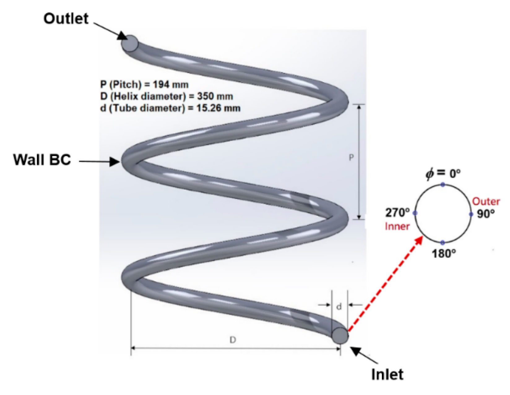
Figure 2.
Different mesh distributions on the cross-section of HCT.
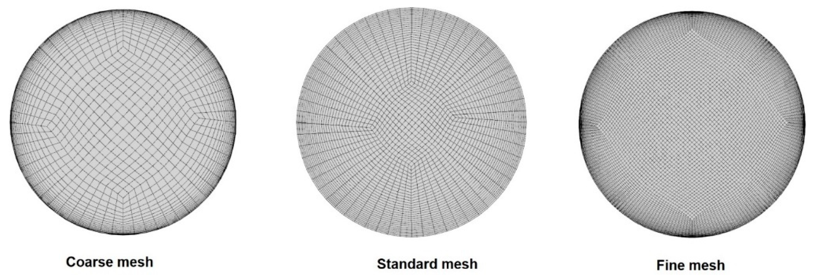
Figure 3.
Effect of different mesh on predicted distributions of wall temperature at x = -0.147 for the Case 1.
Figure 3.
Effect of different mesh on predicted distributions of wall temperature at x = -0.147 for the Case 1.
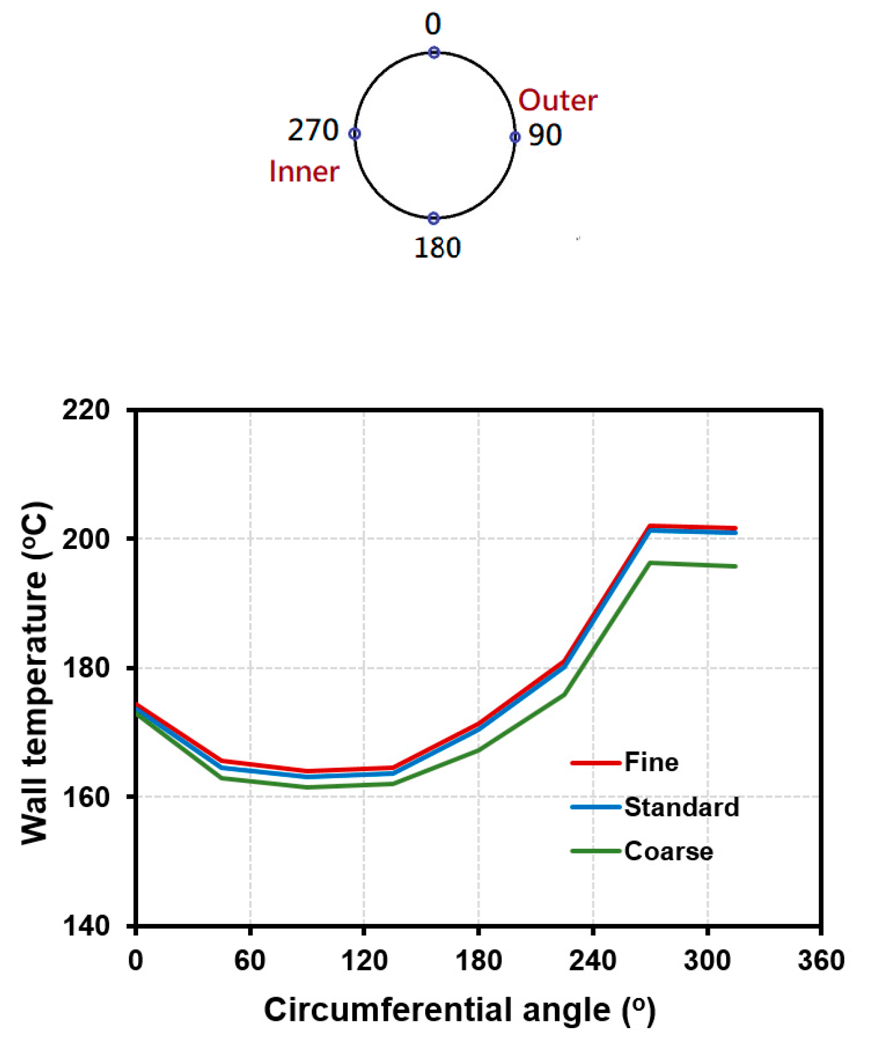
Figure 4.
Effect of different turbulence models on predicted distributions of wall temperature at x = -0.147 for the Case 1.
Figure 4.
Effect of different turbulence models on predicted distributions of wall temperature at x = -0.147 for the Case 1.
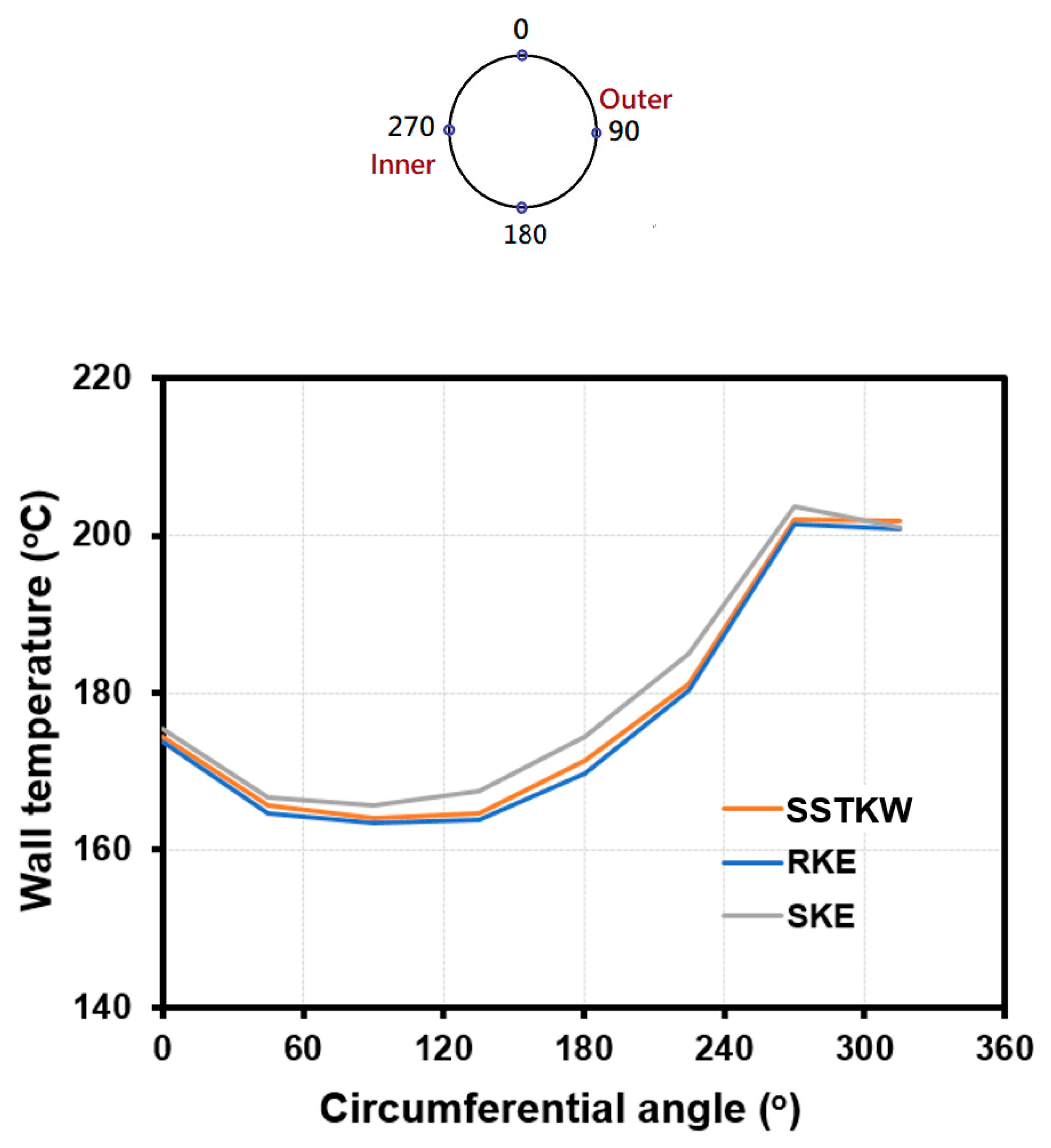
Figure 5.
Comparison of circumferential distribution of wall temperature between predictions and measurements for Case 1.
Figure 5.
Comparison of circumferential distribution of wall temperature between predictions and measurements for Case 1.
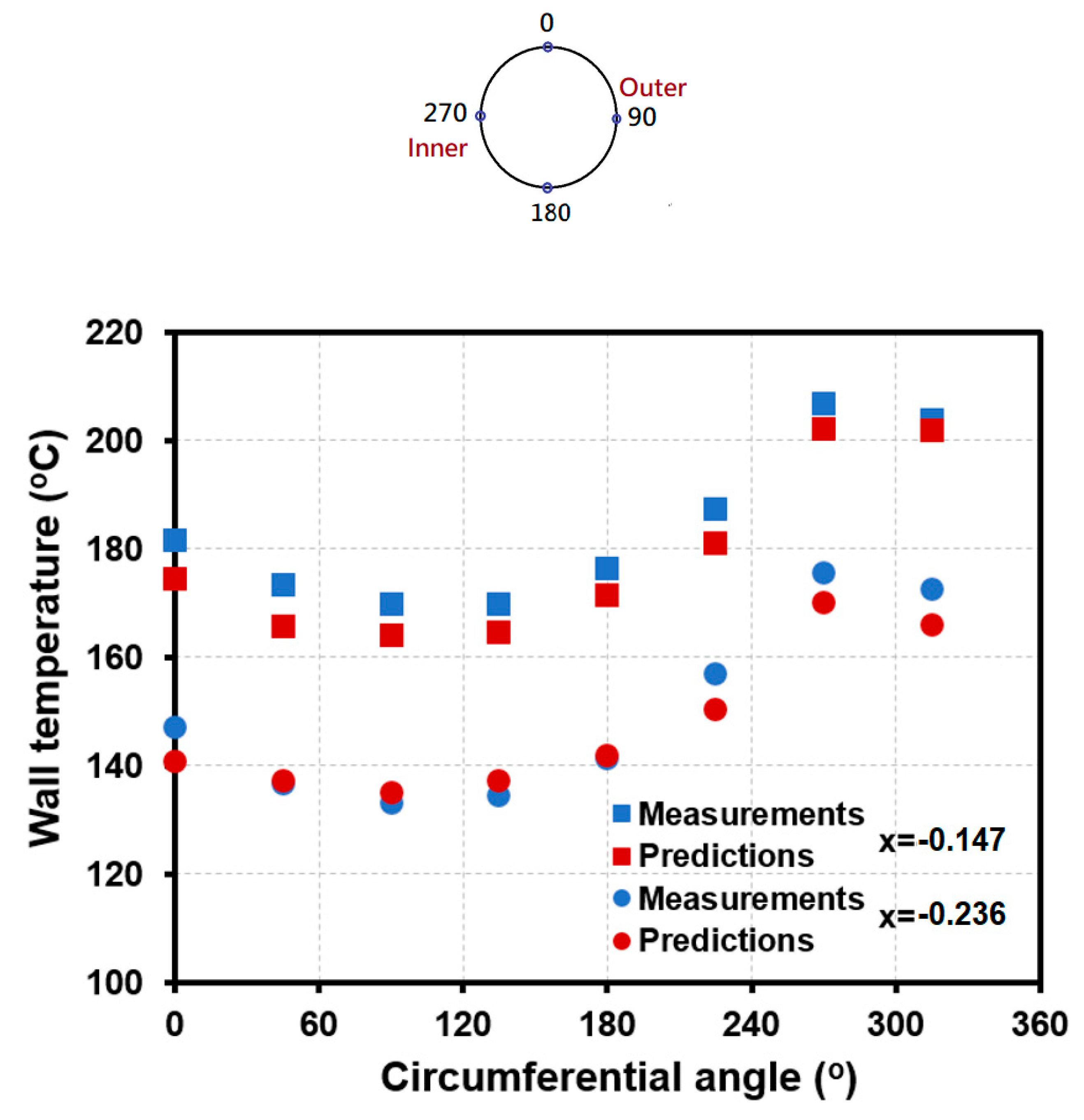
Figure 6.
Density contours on the cross-section of HCT for (a) Case 1; (b) Case 2; (c) Case 3.
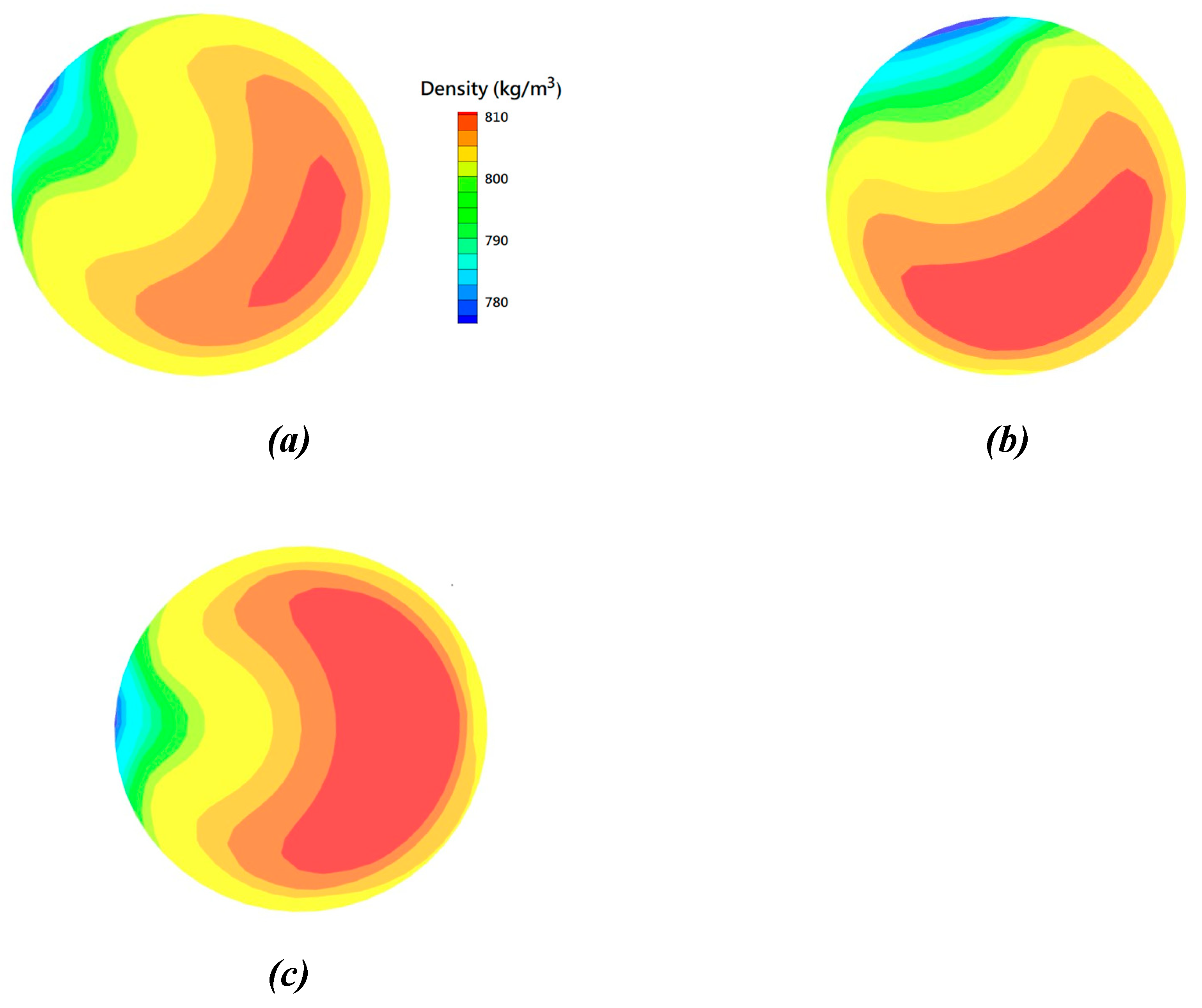
Figure 7.
Comparison of circumferential distribution of wall temperature between predictions and measurements for Case 2 (a) and Case 3 (b).
Figure 7.
Comparison of circumferential distribution of wall temperature between predictions and measurements for Case 2 (a) and Case 3 (b).
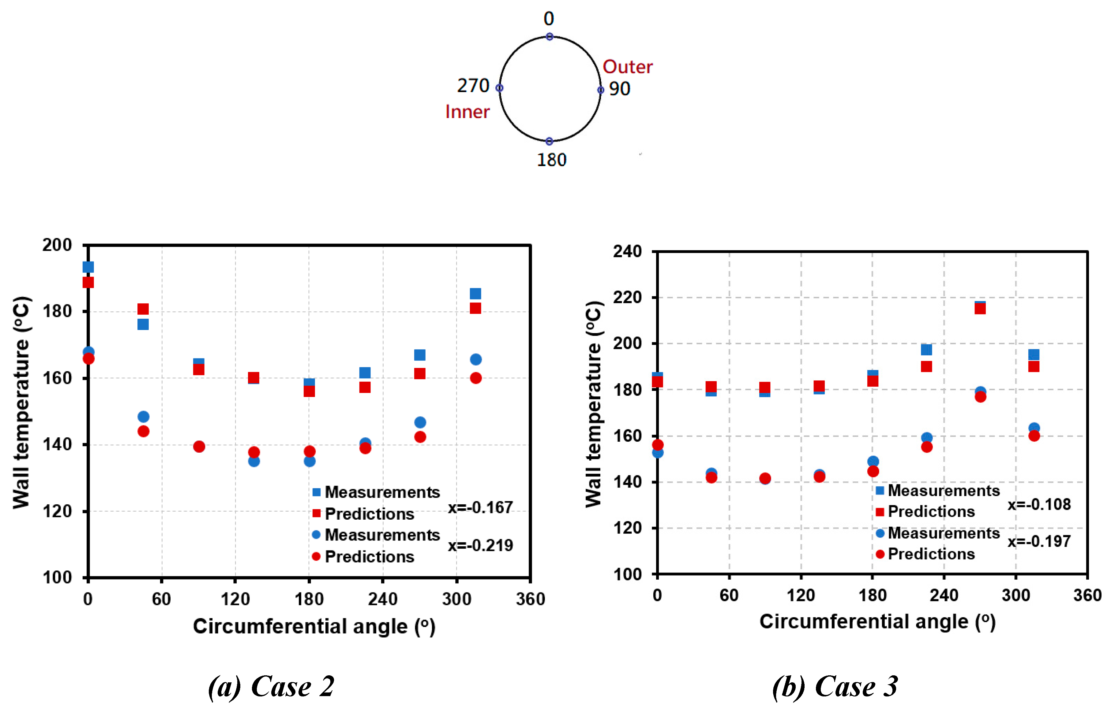
Figure 8.
(a) Vector distributions of secondary flow and temperature contour on the cross-section of HCT for Case 1; (b) Assumed temperature contour in the test; (c) Comparison of predicted and measured wall temperatures for φ = 210o ~330o .
Figure 8.
(a) Vector distributions of secondary flow and temperature contour on the cross-section of HCT for Case 1; (b) Assumed temperature contour in the test; (c) Comparison of predicted and measured wall temperatures for φ = 210o ~330o .
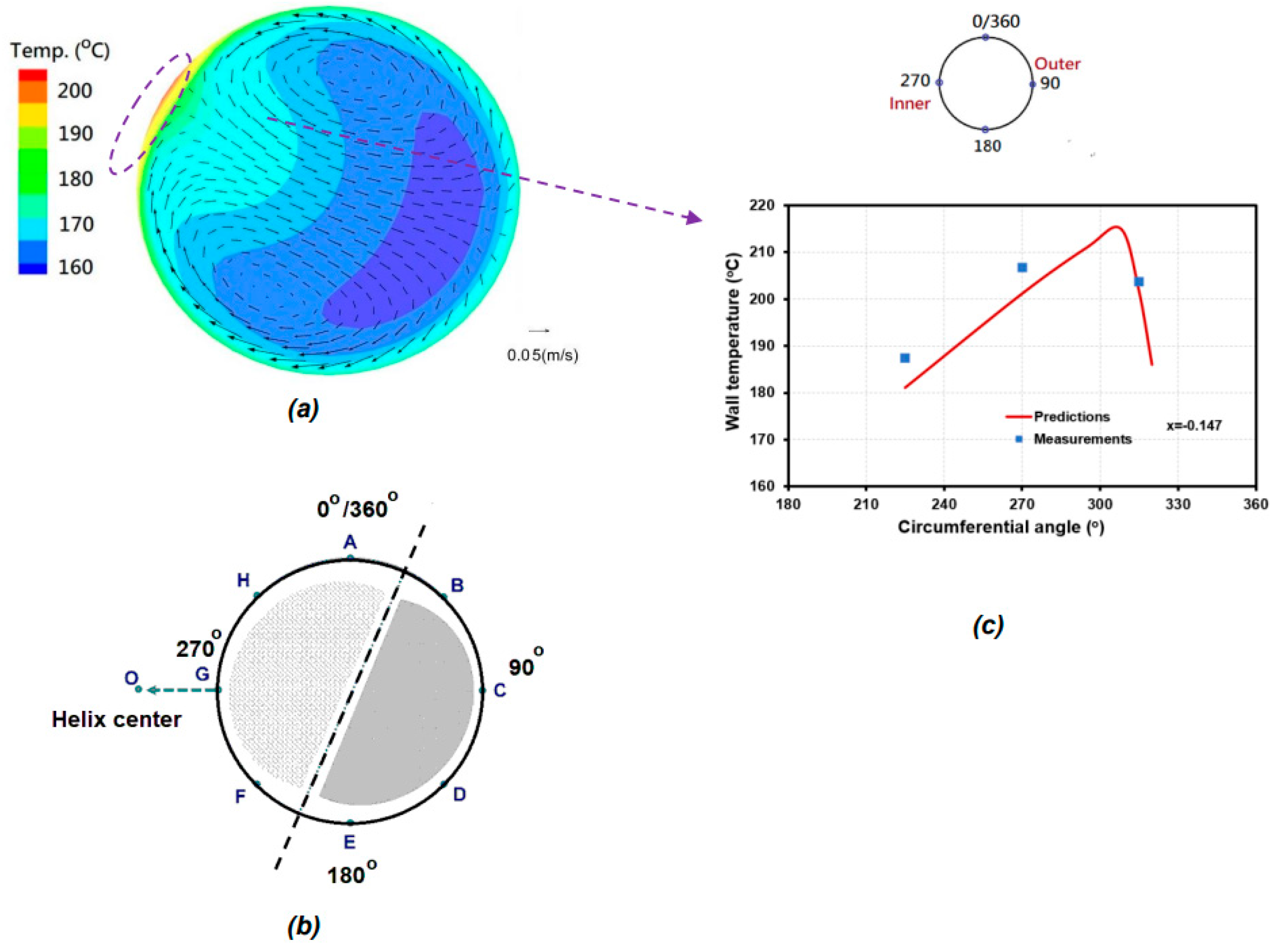
Figure 9.
(a) Vector distributions of secondary flow and temperature contour on the cross-section of HCT for Case 2; (b) Assumed temperature contour in the test; (c) Comparison of predicted and measured wall temperatures for φ = 300o ~410o(50o).
Figure 9.
(a) Vector distributions of secondary flow and temperature contour on the cross-section of HCT for Case 2; (b) Assumed temperature contour in the test; (c) Comparison of predicted and measured wall temperatures for φ = 300o ~410o(50o).
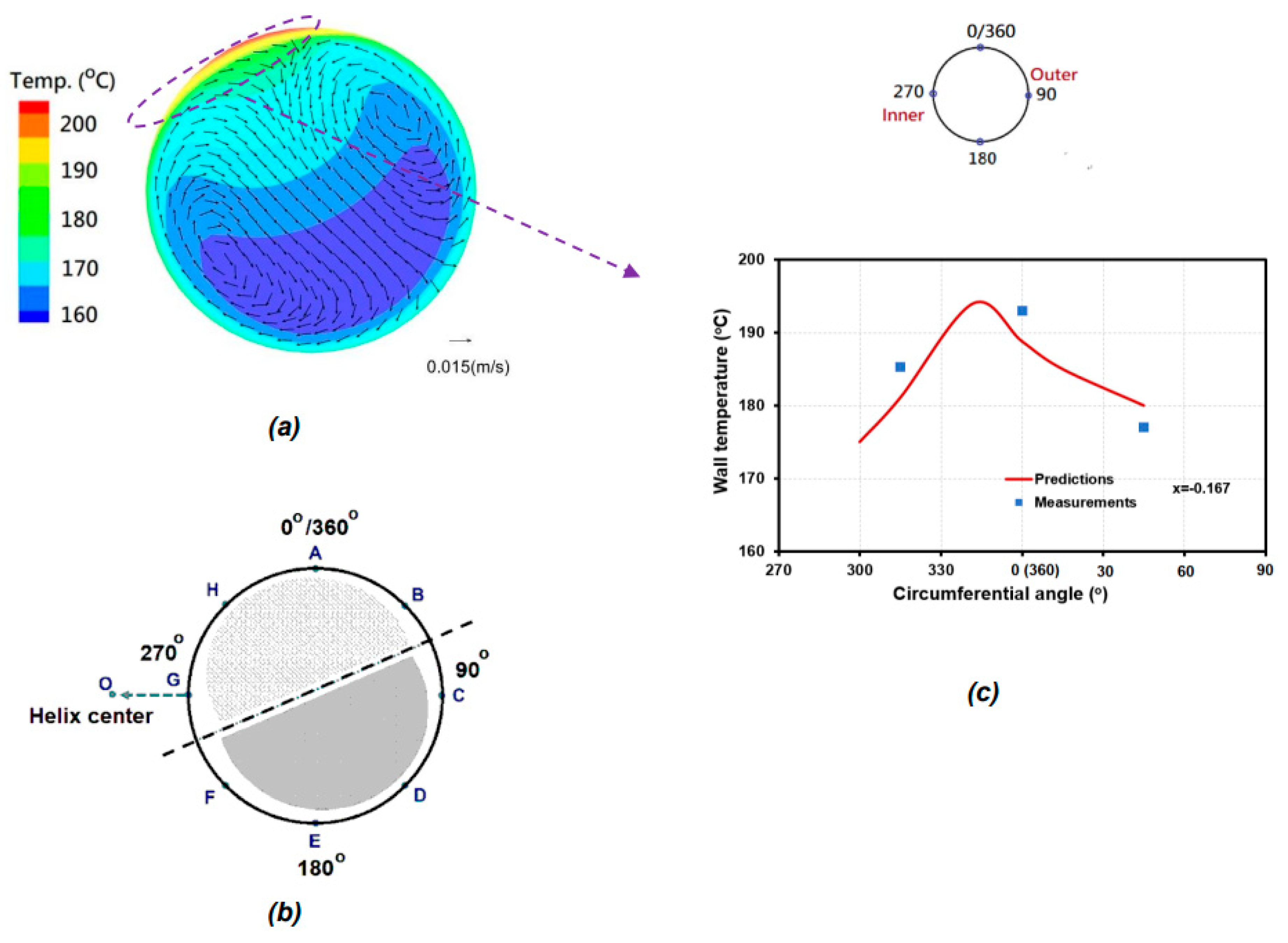
Figure 10.
Comparison of heat transfer coefficients between measurements and predictions for Case 2 (a) and Case 3 (b); (c) Normalized h along HCT.
Figure 10.
Comparison of heat transfer coefficients between measurements and predictions for Case 2 (a) and Case 3 (b); (c) Normalized h along HCT.
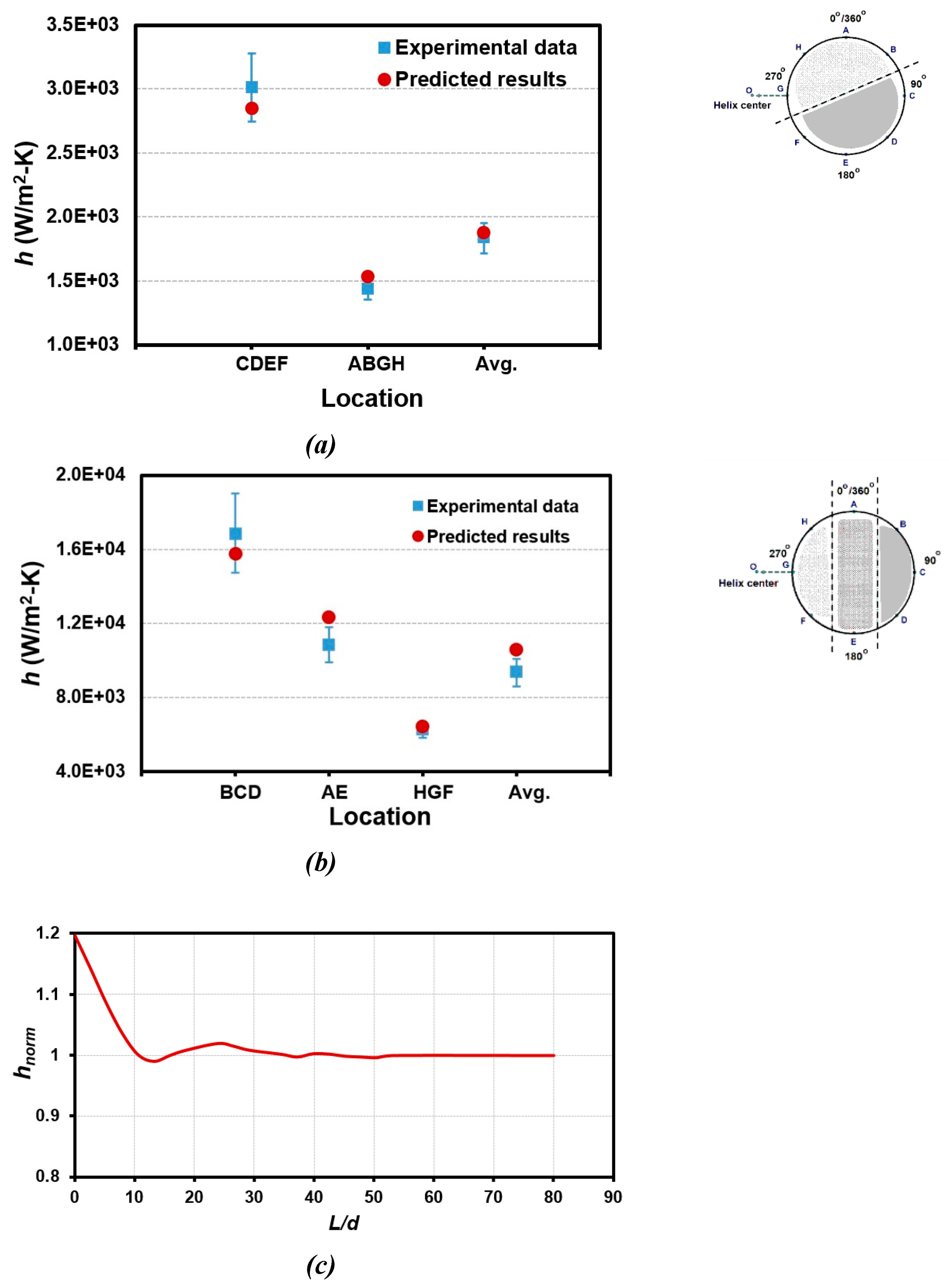
Figure 11.
Comparison of fully-developed h of Case 2 (a) and Case 3 (b) for a HCT obtained from experiment, present model, and correlations.
Figure 11.
Comparison of fully-developed h of Case 2 (a) and Case 3 (b) for a HCT obtained from experiment, present model, and correlations.
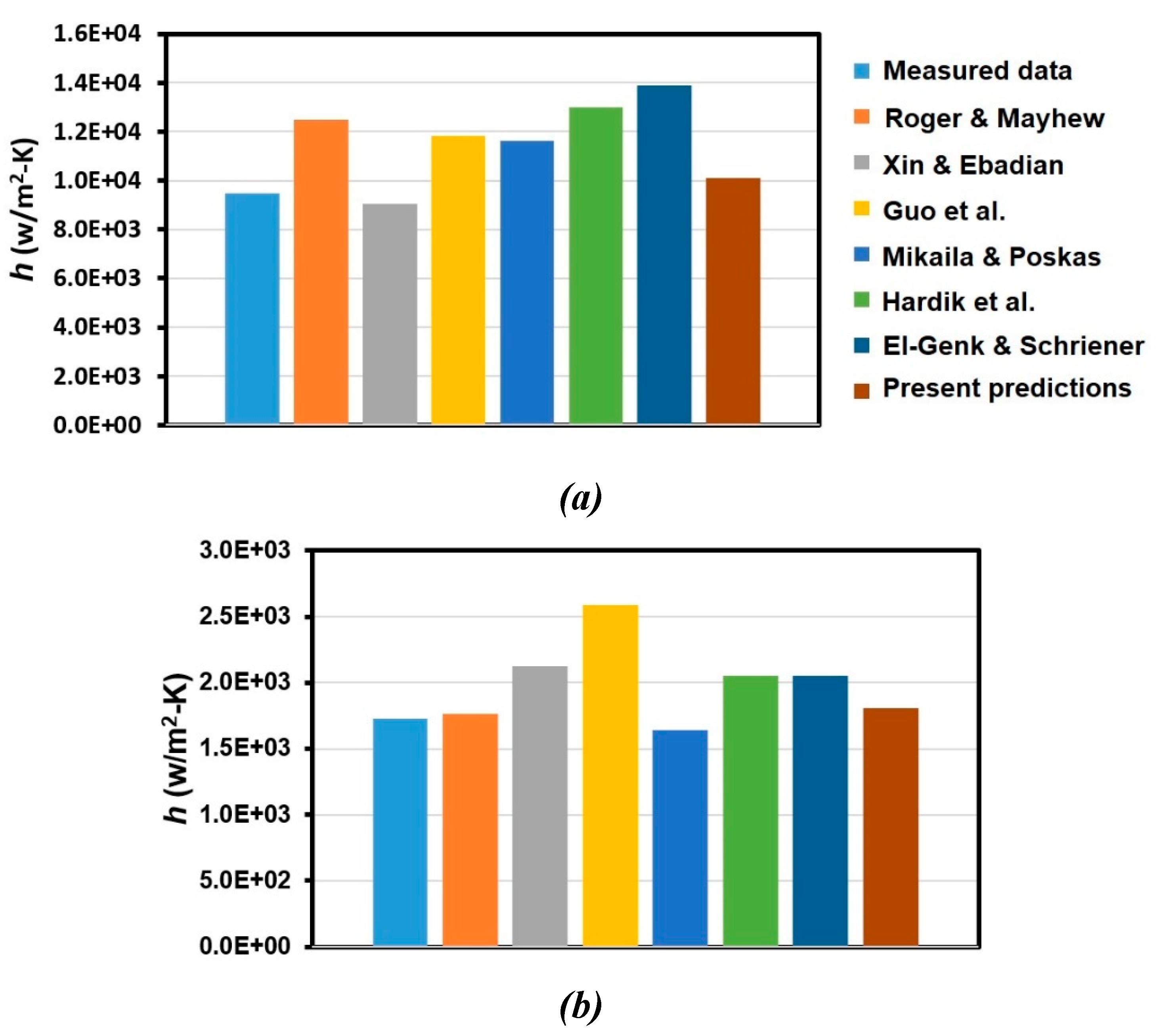
Figure 12.
Comparison of azimuthal dependence of normalized temperature predicted using the constant-heat flux BC and the conjugated-heat-transfer simulation for (a) Case 1; (b) Case 3.
Figure 12.
Comparison of azimuthal dependence of normalized temperature predicted using the constant-heat flux BC and the conjugated-heat-transfer simulation for (a) Case 1; (b) Case 3.
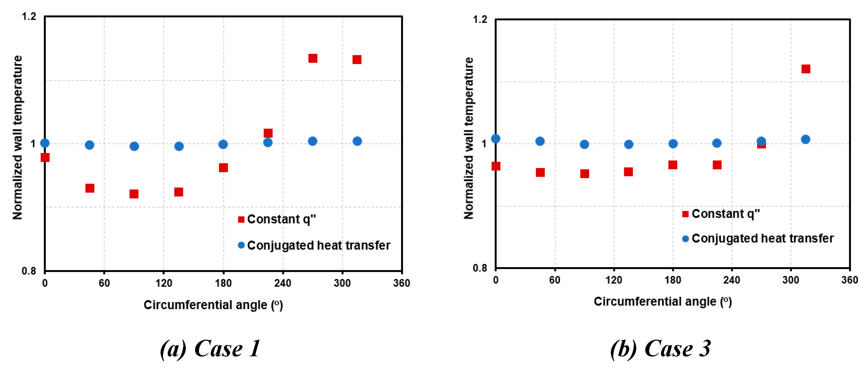

Table 1.
Values of constants in the SSTKW turbulence model.
| 0.85 | 1.176 | 1.0 | 2.0 | 1.168 | 0.31 | 0.075 | 0.0828 | 0.09 | 0.41 | 6 |
Table 2.
Test conditions for all the simulation cases [15].
Table 2.
Test conditions for all the simulation cases [15].
| Mass flux (kg/m2-s) | Heat flux (kW/m2) | Inlet temp. (K) | Pressure (Mpa) | |
|---|---|---|---|---|
| Case 1 | 350 | 150 | 367.15 | 2 |
| Case 2 | 100 | 50 | 367.15 | 2 |
| Case 3 | 1,000 | 245 | 367.15 | 2 |
Disclaimer/Publisher’s Note: The statements, opinions and data contained in all publications are solely those of the individual author(s) and contributor(s) and not of MDPI and/or the editor(s). MDPI and/or the editor(s) disclaim responsibility for any injury to people or property resulting from any ideas, methods, instructions or products referred to in the content. |
© 2025 by the authors. Licensee MDPI, Basel, Switzerland. This article is an open access article distributed under the terms and conditions of the Creative Commons Attribution (CC BY) license (http://creativecommons.org/licenses/by/4.0/).
Copyright: This open access article is published under a Creative Commons CC BY 4.0 license, which permit the free download, distribution, and reuse, provided that the author and preprint are cited in any reuse.


