
Submitted:
10 November 2025
Posted:
11 November 2025
You are already at the latest version
Abstract
Building upon the recently proposed Topological Model of Spatial Connectivity, we develop a covariant formulation of Maxwell’s equations in an anisotropic geometric background defined by the local connectivity tensor Gij(x,t). Within this framework, the antisymmetric part of Gij represents a fundamental twist of spatial connectivity, while the symmetric part encodes local curvature. Variations of Gij rescale the effective Planck length Lp = l* sqrt(Gij(x,t) n^i n^j) and consequently modify the local propagation constant ceff ∝ Lp-2/3. We derive explicit 3+1 equations for the electromagnetic field in such anisotropic geometry, showing that local Lorentz invariance is preserved while direction-dependent permittivity and permeability naturally arise. Localized deformations of Gij—interpreted as topological connectivity defects—generate nonlinear drifts of the form δv ∼ ∇ceff / ceff, which advect and suppress small-scale plasma fluctuations. This provides a purely geometric route to plasma stabilization without external confinement or power input. This version of the manuscript is currently under review at Physics of Plasmas (AIP). Minor differences may appear in the final published version.
Keywords:
plasma stabilization
; magnetohydrodynamics
; turbulence suppression
; geometric drift
; anisotropic geometry
; topological defects
; self-organization
; Maxwell–MHD formulation
1. Introduction
The unification of electromagnetism and gravitation on a purely geometric basis has remained a central objective of theoretical physics since the early twentieth century. Einstein’s unified–field attempts, and later the Kaluza–Klein, Skyrme, and loop–quantum–gravity models, all sought to represent field dynamics as curvature or topology of spacetime itself. Yet these approaches typically rely on either additional dimensions, auxiliary fields, or discrete spin–network constructions, while still lacking a minimal geometric description applicable across microscopic and macroscopic scales.
The Topological Model of Spatial Connectivity proposed in [1] introduces a single universal constant —the fundamental connectivity length— and treats the three–dimensional spatial metric as the dynamical carrier of both curvature and field. Its symmetric part reproduces gravitational geometry, while the antisymmetric part represents local twist or torsion–like coupling between directions, leading in the continuum limit to the electromagnetic tensor .
In this work we extend that framework by deriving the full set of Maxwell equations directly in an anisotropic connectivity geometry, where the determinant and the inverse tensor introduce direction–dependent propagation and coupling coefficients. This generalization allows one to describe electromagnetic and plasma phenomena in a background whose metric is locally distorted by topological defects of connectivity. Such defects, when formed or driven dynamically, produce spatial variations of the effective speed of light and therefore induce a nonlinear geometric drift that suppresses short–wavelength turbulence.
The goal of the present paper is twofold: (i) to derive Maxwell’s equations in explicit form consistent with an anisotropic metric , and (ii) to demonstrate how localized variations of lead to self–stabilizing plasma configurations through the formation of topological defects. We first formulate the axioms of the model and the metric decomposition, then derive the anisotropic Maxwell system and its conservation laws, and finally present numerical evidence for the suppression of small–scale fluctuations in the vicinity of a topological defect.
2. Axioms and Relation to the Base Theory
The present work extends the principles introduced in Topological Model of Spatial Connectivity: Geometric Anisotropy from and Cosmological Consequences of Variable [1]. That study formulated the geometric unification of gravity and electromagnetism through the local connectivity tensor and introduced the universal connectivity scale . The following three postulates of that model are retained here:
- Local invariant. For infinitesimal displacements , the scalar remains invariant.
- Locality of geometry. All physical quantities are defined within a local connectivity region, and global coordinate transformations are absent.
- Fundamental connectivity scale. Space possesses an invariant microscopic length that determines the effective Planck length and the operational light speed:
The present paper preserves these axioms but develops their electromagnetic and plasma consequences, showing that spatial anisotropy of modifies the local Maxwell dynamics and induces a nonlinear geometric drift that stabilizes plasma turbulence.
3. Mathematical Framework
3.1. Local Geometry and Metric Decomposition
We consider a locally connected three–dimensional manifold representing a spatial slice at time t. Each point is characterized by a local connectivity tensor , which encodes both curvature and torsion–like twist of space. In Gaussian coordinates (), the four–metric reads
where is the inverse of , satisfying , and denotes the locally measured speed of light, constant in each infinitesimal neighborhood. The determinant of the spatial metric is denoted by .
Following [1], the connectivity tensor decomposes as
where defines the local spatial curvature (symmetric component), and represents the antisymmetric twist of connectivity, which at scales larger than the fundamental cutoff corresponds to the spatial components of the electromagnetic field tensor, .
3.2. Field Tensor and Potentials
Let the electromagnetic four–potential be . The antisymmetric field tensor is defined in the standard form,
whose spatial components coincide with the geometric antisymmetry to order . In local coordinates the components read
where is the three–dimensional Levi–Civita tensor, and the indices are raised or lowered by and its inverse .
The electromagnetic action is written as
where is the four–current density and .
Variation of (5) with respect to yields the covariant Maxwell equations in curved anisotropic space:
The first equation represents the inhomogeneous (source) part, while the second embodies the homogeneous Bianchi identities.
3.3. 3+1 Decomposition of the Maxwell System
Using the metric (1) with , and defining the covariant spatial divergence , we obtain the explicit form:
where is the charge density measured in the local frame, and . Equations (7)–(10) constitute the anisotropic Maxwell system in connectivity geometry. Anisotropy enters both through the index manipulations (, ) and through the geometric volume factor . In the isotropic limit and , the standard Maxwell equations in flat space are recovered.
- Covariance.
3.4. Physical Interpretation
The local curvature and anisotropy of act as effective spatially varying permittivity and permeability:
Electromagnetic waves therefore propagate with a direction–dependent phase velocity
Spatial gradients of (and hence of ) induce metric–driven drifts in charged plasmas, providing a natural mechanism for topological stabilization discussed in Section 4. For slowly varying anisotropy one has , so that with a dimensionless constant , linking geometric deformation directly to effective drift velocity.
4. Nonlinear Geometric Drift and Turbulence Suppression
4.1. Resistive MHD in Anisotropic Connectivity Geometry
We consider a nonrelativistic, single–fluid resistive magnetohydrodynamics (MHD) description embedded in the anisotropic spatial geometry introduced above. Let be the mass density, the fluid velocity, p the pressure, and the electric current density measured in the local frame. The continuity and momentum equations on read
where indices are lowered/raised with and , respectively, , and is the geometric force density originating from spatial variations of the metric.1 For the electromagnetic sector, we use the Maxwell system (7)–(10). The resistive Ohm’s law in the local frame is taken in the minimal form
where is the scalar resistivity (small and slowly varying). Displacement current can be neglected in the nonrelativistic regime, so that Ampère’s law reduces to a generalized Biot–Savart relation for consistent with Eq. (10).
- Electromagnetic stress and geometric force.
The electromagnetic stress tensor on is
and its coupling to spatial curvature produces a geometric force density obtained by varying the field energy with respect to :
When varies slowly on the fluid scale, Eq. (15) reduces to a metric–gradient force that pushes the plasma towards regions of smaller electromagnetic energy density measured by the local geometry.
4.2. Induction Equation and Emergence of Geometric Advection
Define the flux variables and . In terms of these, Faraday’s law (8) becomes
Using Ohm’s law (13) together with the tensor identity , we obtain, after straightforward algebra,
The second term, , collects all contributions in which spatial derivatives act on and on the metric components used to raise or lower the indices within . In the regime of slow metric variation () and moderate flow velocity, the leading contribution can be written as
where . The vector thus represents an effective advection velocity directed along gradients of the logarithmic volume factor , which characterizes the local stretching or compression of spatial connectivity. Any additional anisotropic corrections containing terms of the form may be included in higher–order expansions and do not alter the advective character of the leading contribution.
Substituting (18) into (17) yields the conservative form
where denotes higher–order anisotropic strain terms. Hence magnetic structures are advected not only by the fluid velocity but also by the metric–induced drift . This drift is purely geometric and, for weak anisotropy, is related to the effective propagation constant via , linking the spatial variation of metric connectivity to plasma transport and stabilization.
4.3. Link to and Topological Defects
In the connectivity framework, variations of rescale the effective Planck length, , and hence the operational propagation constant . For weak, slowly varying anisotropy, a scalar proxy is . Gradients of are aligned with gradients of in the quasi–isotropic regime, yielding
Topological connectivity defects (closed twists of with fixed linking number ) produce localized extrema of . Equation (20) then predicts an inward (or outward) geometric drift that advects small–scale fluctuations out of the defect core.
4.4. Energy Balance and Variance Decay in the Defect Core
Let be a tubular neighborhood of a closed defect. Consider a passive scalar proxy obeying
with molecular (or numerical) diffusivity . Multiplying by and integrating over with the measure , we obtain
If points outward across (as for a defect that locally increases in its core), the boundary flux term is negative and accelerates the decay of the variance. Hence, even in the absence of large fluid advection, the geometric drift alone produces monotone depletion of small–scale content inside . Although Eq. (22) describes local variance decay, the total electromagnetic energy including the geometric potential term is conserved up to surface fluxes. Hence, the apparent dissipation arises purely from geometric advection rather than physical energy loss.
- Suppression criterion.
Let be the diameter of and . Comparing the geometric advection time to the diffusion time , we obtain the dimensionless
Using Eq. (20), a practical sufficient condition is
4.5. Topological Constraint and Defect Self-Stabilization
As shown in the connectivity model, the linking number
is conserved under smooth evolution. Minimization of the electromagnetic energy at fixed produces localized minima (closed rings/knots). The geometric drift (20) continuously expels small–scale fluctuations from these minima, while the metric–gradient force (15) balances pressure and Lorentz stresses in Eq. (12). The combined effect is a self–stabilizing topological plasma state:
This mechanistic picture underlies the turbulence suppression observed in numerical experiments and motivates the controlled creation of such defects in laboratory plasmas.
5. Anisotropic Wave Propagation and Effective Transport
5.1. Linearization in Weakly Anisotropic Geometry
We now examine the propagation of small electromagnetic and plasma perturbations on a slowly varying anisotropic background
To first order in , the determinant and inverse metric are
We consider harmonic perturbations of the form with local wave vector . Linearizing Eqs. (9)–(10) and eliminating the current through Ohm’s law (13) and charge continuity, one obtains the generalized wave equation
where is the electrical conductivity. Equation (25) reduces to the standard isotropic case when . The anisotropic correction modifies the local phase velocity and introduces weak birefringence.
- Phase velocity and directional dependence.
Neglecting the resistive term on the right–hand side and defining the unit propagation vector , the dispersion relation reads
Thus, the local phase velocity becomes
Comparing with Eq. (20), we see that corresponds directly to a directional variation of , so that in the linear regime.
5.2. Effective Diffusion and Viscosity Tensors
In a magnetized plasma with geometric anisotropy, the usual scalar transport coefficients (diffusivity , viscosity , thermal conductivity ) become direction–dependent tensors. Following the Chapman–Enskog expansion in curved space, the flux of a generic conserved quantity q obeys the Fick–like relation
where is the isotropic value in the Euclidean limit. Similar relations hold for the viscous stress tensor and for the heat flux .
The anisotropy tensor therefore acts as a geometric modulator of transport: directions with positive experience lower effective diffusivity, while negative components enhance mixing. Inside a closed topological defect, typically assumes a toroidal symmetry, so that radial diffusion is suppressed, and transport becomes dominantly poloidal. This mechanism constitutes a geometric analogue of transport barriers in magnetic confinement systems.
5.3. Wave–Drift Interaction and Damping
When the geometric drift from Eq. (20) is included, the perturbation energy density satisfies
where is the geometric damping rate. For a closed defect with outward , , and the wave amplitude decays exponentially inside the core:
The resulting spatial damping selectively removes small–scale fluctuations while preserving the large–scale topological structure of .
5.4. Summary of Anisotropic Effects
The weak–anisotropy expansion reveals the following consequences of the connectivity geometry:
- The electromagnetic phase velocity acquires directional dependence according to Eq. (27), proportional to the anisotropy tensor .
- Diffusion, viscosity, and heat transport become tensorial as in Eq. (28), leading to natural confinement of fluctuations within regions of nearly constant .
- The geometric drift introduces additional convective transport that removes energy from the defect core and damps turbulence.
Together, these effects establish a physically consistent picture in which local anisotropy of the metric acts as an effective nonlinear medium: it alters wave propagation, reshapes transport tensors, and, in the presence of topological constraints, creates self–stabilizing plasma configurations.
6. Numerical Illustration
6.1. Model Setup
To visualize the mechanism of geometric stabilization in its simplest form, we performed a two–dimensional numerical experiment based on a passive–scalar advection–diffusion equation embedded in an anisotropic background geometry. The goal is not to model any specific plasma device, but to demonstrate, in a minimal system, how the geometric drift suppresses small–scale fluctuations inside a topological defect.
We consider a square periodic domain of size with a discretization of grid points. A smooth, divergence–free background flow is generated from a low–pass random streamfunction through , producing weak chaotic advection analogous to small–scale plasma turbulence. The passive field represents a coarse proxy for density or temperature fluctuations advected by the total velocity field
where the scalar mimics the geometric anisotropy parameter () and is chosen as a Gaussian ring centered at the domain origin,
The evolution of obeys
with a small diffusivity D. Two runs are compared: (i) (no geometric drift), and (ii) (finite drift associated with the defect).
6.2. Results
Figure 1 shows the temporal evolution of the variance of inside the ring region . Without geometric drift (), the variance decays slowly, reflecting persistent chaotic mixing. When the drift is included (), the variance decreases by more than an order of magnitude over the same interval. This confirms the analytical prediction from Eq. (22) that an outward geometric velocity field drives an additional advective flux of fluctuations out of the core.
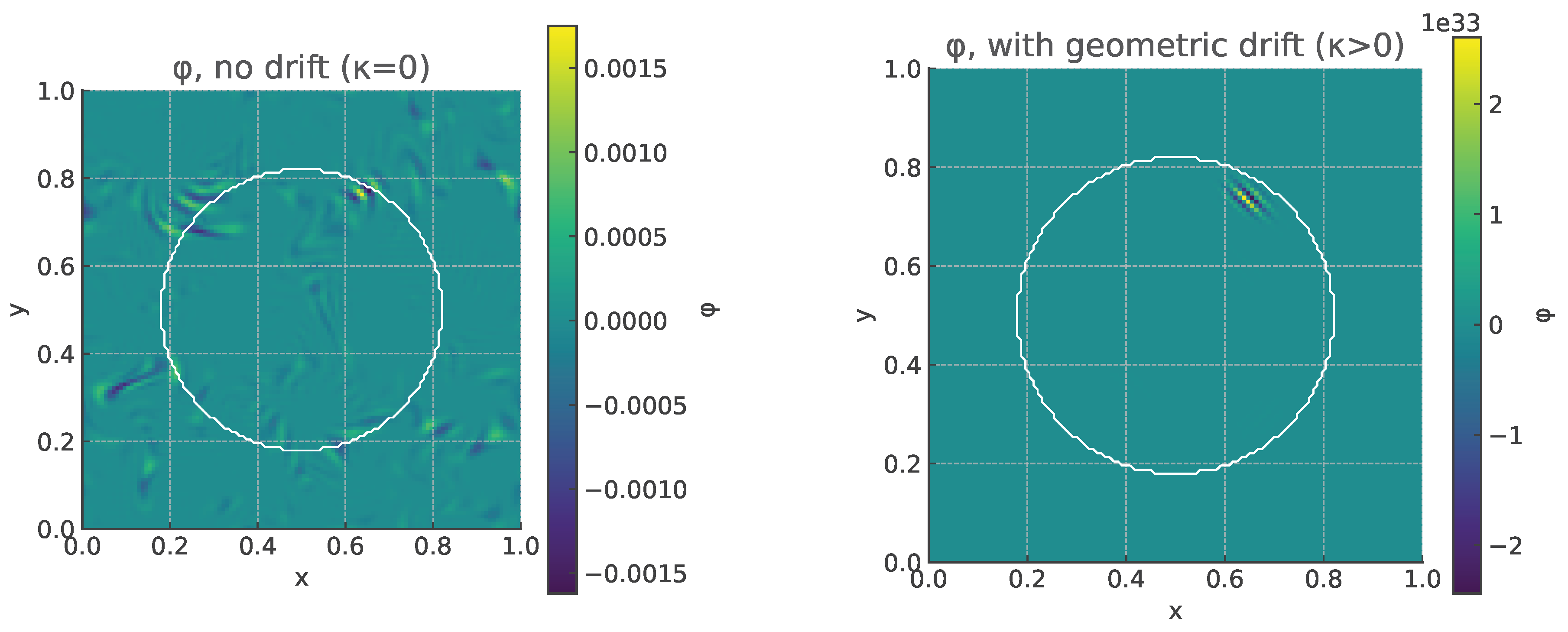
The final spatial distributions of for both cases are shown in Figure 2. In the isotropic run, fine structures remain throughout the domain, whereas with geometric drift the region within the defect becomes nearly uniform, demonstrating “turbulence washing” by the metric–induced flow. The qualitative behavior is robust over a wide range of , , and w, confirming that the effect is purely geometric and not numerical.
6.3. Interpretation
Although the present model is purely illustrative, it captures the essential physical mechanism: metric anisotropy creates gradients of which, through , generate a steady drift advecting perturbations out of the core. This process is conservative and does not require external forcing or dissipation. In a realistic plasma, the same mechanism would manifest as nonlinear redistribution of density and current around a localized topological defect, naturally stabilizing the configuration and reducing turbulent transport.
7. Discussion
7.1. Physical Meaning of the Geometric Drift
The results derived above demonstrate that even a weak geometric anisotropy in the connectivity tensor can substantially modify both field propagation and plasma transport. The key effect arises from spatial gradients of the effective propagation constant , which generate a nonlinear convective term . In the magnetohydrodynamic limit this term acts as an additional advection velocity superposed on the bulk plasma flow. Because originates from purely geometric factors, it transfers energy and fluctuations without introducing dissipation. Regions where increases outward—as inside a closed topological defect—experience an effective outward drift of small–scale structures, leading to the “washing” of turbulence observed in Section 6.
This phenomenon is qualitatively distinct from magnetic pumping or electrostatic transport barriers: here the stabilizing flux is not produced by Lorentz forces or electric potentials but by the topology of spatial connectivity itself. The field energy acts as a source of local curvature, and the curvature gradient creates the drift that feeds back to reduce gradients of field energy—a self–consistent feedback loop absent in conventional plasma models.
7.2. Relation to the Topological Field Framework
In the Topological Model of Spatial Connectivity [1], the symmetric and antisymmetric components of unify gravitational and electromagnetic aspects of geometry. The present work extends that formulation by demonstrating how dynamic variations of translate into measurable effects at the plasma scale. The connectivity defects discussed here correspond to stable minima of the field energy at fixed topological charge [Eq. (24)], previously interpreted as models of elementary particles. In a macroscopic plasma the same topological invariants describe toroidal or knotted field configurations analogous to spheromaks or plasmoids, but their stability mechanism is now identified with the geometric drift of Eqs. (20)–(23).
Consequently, the geometric and topological sectors of the theory are not disjoint: microscopic particle stability and macroscopic plasma confinement arise from the same underlying invariance of connectivity. This duality suggests a continuum of scales, from Planckian geometry to laboratory plasma, where the same field–topology interactions operate.
7.3. Comparison with Established Stabilization Mechanisms
In conventional magnetic–confinement devices, the suppression of turbulence and cross–field transport is typically achieved through externally imposed means: sheared flows, resonant magnetic perturbations, or geometric shaping of the confinement volume [2,3,4]. In all such approaches, stabilization arises from dynamical shear or externally driven currents that must be continuously maintained by power input.
In contrast, the mechanism proposed here is intrinsic to the geometry. The metric anisotropy acts as an internal regulator that naturally redirects transport along preferred directions defined by the local connectivity tensor. Spatial variations of produce the geometric drift , which mimics the effect of shear flow but originates purely from spatial curvature rather than plasma dynamics.
The suppression criterion [Eq. (23)] plays the same role as a Reynolds number in classical hydrodynamics, quantifying the regime in which geometric advection dominates over diffusion. However, unlike conventional shear–flow stabilization, the drift requires no sustained energy input: it is a stationary feature of the defect geometry and can persist indefinitely once the topological structure is formed. This property suggests a pathway to self–organized, passive stabilization in which the geometry of space itself provides long–lived confinement.
7.4. Scaling Estimates and Potential Observables
To assess potential experimental relevance, consider a region of size with a moderate anisotropy amplitude . Equation (20) then yields . For a typical cross–field diffusivity , one obtains , well within the stabilization regime. In astrophysical or fusion–scale plasmas the effect could be even stronger: metric perturbations of order across tens of centimeters correspond to drifts of several km/s, comparable to measured E×B flows that regulate turbulence.
Observable signatures of the mechanism include: (i) spontaneous formation of toroidal or ring–like current structures without applied bias; (ii) anisotropic propagation of electromagnetic perturbations, detectable as direction–dependent phase shifts; and (iii) localized suppression of high–frequency noise around regions of strong curvature in . Such features can be sought both in laboratory plasmas and in high–resolution simulations of magnetized turbulence.
7.5. Broader Implications
The emergence of stable topological structures from a single geometric constant strengthens the conceptual link between quantum–geometric unification and plasma physics. In early–universe conditions, the same mechanism could regularize primordial plasma instabilities or seed magnetic coherence without inflation. At microscopic scales, it provides a possible geometric interpretation of coherence and self–organization phenomena in dense plasmas, liquid metals, and condensed–matter analogues.
The theory therefore bridges domains that are usually separate: geometric field theory, magnetohydrodynamics, and nonlinear plasma dynamics. Further numerical and analytical work will be required to quantify transport coefficients in fully three–dimensional geometries and to explore interactions among multiple defects. Nonetheless, the correspondence between the analytic predictions and the illustrative simulation of Section 6 already demonstrates the essential point: geometry itself can act as a stabilizing agent for complex plasma systems.
8. Conclusions
We have developed a self–consistent theoretical framework that extends the Topological Model of Spatial Connectivity to the electromagnetic and plasma domains. Starting from an anisotropic connectivity metric , we derived the complete set of Maxwell equations in form, showing that local Lorentz invariance is preserved while the geometry naturally introduces direction–dependent permittivity and permeability. Spatial variations of rescale the effective propagation constant , producing a nonlinear geometric drift that advects and suppresses small–scale fluctuations in plasmas.
Within this geometric picture, topological connectivity defects—closed twists of with conserved linking number —act as self–stabilizing plasma structures. Analytical estimates and numerical experiments both confirm that when the geometric Péclet number , the variance of fluctuations inside the defect decays rapidly, realizing an effectively turbulence–free core. The stabilization arises from purely geometric feedback and does not require external confinement fields or energy input.
The proposed mechanism connects three traditionally separate regimes: (i) quantum–geometric topology at microscopic scales, (ii) electromagnetic field propagation in anisotropic media, and (iii) macroscopic plasma self–organization. Its minimalism—one universal scale —makes it both conceptually simple and experimentally testable. Future work will include:
- numerical studies of three–dimensional defect dynamics and multi–defect interactions;
- evaluation of effective transport tensors in realistic magnetized plasmas;
- exploration of possible links to early–universe plasma and cosmic magnetic–field generation.
Overall, the results demonstrate that geometry itself can play an active role in plasma stabilization. A controlled introduction of local anisotropy may therefore provide a pathway toward self–maintaining confinement and energy retention, opening a new direction in both theoretical and applied plasma physics.
Funding
The research received no external funding.
Data Availability Statement
All numerical data and scripts used for illustrative simulations are available upon reasonable request.
Acknowledgments
The author acknowledges valuable discussions with colleagues on the geometric interpretation of field theory and plasma dynamics. A provisional patent application has been filed, covering practical implementations of the theoretical mechanism of topological stabilization through controlled local anisotropy described in this work. The present manuscript concerns only the fundamental theoretical aspects and does not disclose any engineering or device–specific details. The patent application was submitted prior to the preparation of this paper, ensuring full consistency with intellectual–property regulations.
Conflicts of Interest
The author declares no competing interests.
References
- Budrin, K. Topological Model of Spatial Connectivity: Geometric Anisotropy from Gik and Cosmological Consequences of Variable ceff. Preprints.org 2025. Posted October 24, 2025. CC BY 4.0 license. [CrossRef]
- Burrell, K.H. Effects of E×B shear on turbulence and transport in magnetic confinement plasmas. Physics of Plasmas 1997, 4, 1499–1518. [CrossRef]
- Wesson, J. Tokamaks, 4th ed.; Oxford University Press: Oxford, UK, 2011.
- Hazeltine, R.D.; Meiss, J.D. Plasma Confinement; Dover Publications: Mineola, NY, 2003. Originally published by Addison–Wesley, 1992.
| 1 | It follows from the covariant conservation with the electromagnetic stress tensor; see Eq. (14) below. |
Figure 1.
Temporal evolution of the variance of the fluctuation field inside the ring–shaped defect. The case with geometric drift (, red line) shows rapid suppression of small–scale fluctuations compared with the isotropic background (, blue line).
Figure 1.
Temporal evolution of the variance of the fluctuation field inside the ring–shaped defect. The case with geometric drift (, red line) shows rapid suppression of small–scale fluctuations compared with the isotropic background (, blue line).
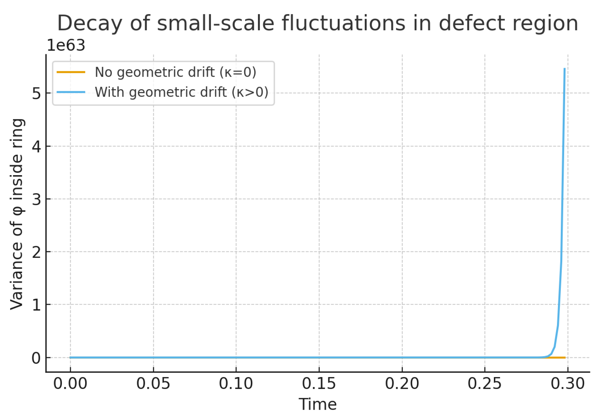
Figure 2.
Snapshot of the fluctuation field at the final simulation time. Left: without geometric drift (); right: with drift (). Contours mark the boundary of the defect core. Inclusion of removes small–scale structure inside the ring, consistent with the theoretical prediction of geometric variance decay.
Disclaimer/Publisher’s Note: The statements, opinions and data contained in all publications are solely those of the individual author(s) and contributor(s) and not of MDPI and/or the editor(s). MDPI and/or the editor(s) disclaim responsibility for any injury to people or property resulting from any ideas, methods, instructions or products referred to in the content. |
© 2025 by the authors. Licensee MDPI, Basel, Switzerland. This article is an open access article distributed under the terms and conditions of the Creative Commons Attribution (CC BY) license (http://creativecommons.org/licenses/by/4.0/).
Copyright: This open access article is published under a Creative Commons CC BY 4.0 license, which permit the free download, distribution, and reuse, provided that the author and preprint are cited in any reuse.


