
Submitted:
10 November 2025
Posted:
12 November 2025
You are already at the latest version
Abstract
Water Alternating Gas (WAG) injection is a well-established enhanced oil recovery technique that improves sweep efficiency by combining the favorable displacement characteristics of waterflooding and gas injection. This work presents a sequential Picard–Newton formulation for simulating three-phase flow under WAG conditions in heterogeneous petroleum reservoirs. The mathematical model considers slightly compressible, immiscible oil, water, and gas phases under isothermal conditions, discretized using the finite volume method. Reservoir heterogeneity is represented through geostatistical permeability fields generated by Sequential Gaussian Simulation, capturing the spatial correlations and anisotropy characteristic of subsurface formations. The methodology is applied to investigate WAG performance in two heterogeneous reservoir models with mean permeabilities of 100 mD and 200 mD under identical 1:1 injection ratios. The numerical results successfully reproduce the cyclic saturation and production behavior characteristic of WAG processes. Comparative analysis reveals that higher permeability enhances injectivity and cumulative recovery but accelerates water breakthrough and production decline, illustrating the trade-off between displacement efficiency and sweep control. These findings demonstrate that the proposed framework provides an efficient and physically consistent tool for evaluating WAG strategies in heterogeneous reservoirs, with potential application to field-scale optimization of advanced recovery operations.
Keywords:
enhanced oil recovery
; finite volume method
; heterogeneous reservoirs
; Picard-Newton method
; Sequential Gaussian Simulation Method
; WAG injection
1. Introduction
Enhanced Oil Recovery (EOR) techniques have become increasingly critical for maximizing hydrocarbon production from mature and unconventional reservoirs, where primary and secondary recovery methods have reached their economic limits. As global energy demands continue to rise while easily accessible oil reserves decline, the petroleum industry faces mounting pressure to develop more efficient and cost-effective recovery strategies [1,2,3]. Among the various EOR approaches, including chemical, thermal, and miscible gas injection methods, Water Alternating Gas (WAG) injection has emerged as one of the most widely implemented and technically proven techniques for enhancing oil recovery in both onshore and offshore operations [4,5].
The WAG process addresses fundamental limitations inherent in conventional water flooding and gas injection schemes. Pure water injection, while effective in maintaining reservoir pressure and displacing oil, often suffers from viscous fingering and poor sweep efficiency due to unfavorable mobility ratios between water and oil phases. Conversely, gas injection, particularly CO2 flooding, can achieve excellent displacement efficiency through miscible or near-miscible interactions with reservoir fluids, but is prone to gravity override and channeling effects that significantly reduce volumetric sweep efficiency [6,7]. By alternating the injection of water and gas slugs, WAG injection combines the mobility control benefits of water flooding with the displacement efficiency advantages of gas injection, resulting in improved overall recovery performance [8,9].
The effectiveness of WAG processes depends on numerous factors, including reservoir heterogeneity, fluid properties, injection strategy parameters (such as WAG ratio, slug size, and injection rates), and operational constraints. Reservoir heterogeneity, in particular, plays a crucial role in determining the success of WAG operations, as permeability variations can lead to preferential flow paths that compromise sweep efficiency and ultimate recovery [10,11]. Understanding and predicting the complex interactions between these factors requires sophisticated numerical modeling capabilities that can accurately capture the physics of three-phase flow in heterogeneous porous media.
Indeed, numerical simulation has become an indispensable tool for the design, optimization, and risk assessment of EOR strategies, providing a cost-effective and safe alternative to extensive field trials [12,13]. However, modeling three-phase flow in heterogeneous reservoirs presents significant computational challenges due to the strongly nonlinear nature of the governing equations, the presence of sharp saturation fronts, and the need to accurately represent complex geological features across multiple length scales. The coupled system of mass conservation equations for oil, water, and gas phases, combined with modified Darcy’s law and appropriate constitutive relationships, results in a highly nonlinear system of partial differential equations that requires robust and efficient numerical solution strategies [14,15].
Traditional numerical approaches for reservoir simulation can be broadly classified into two categories: fully implicit methods (FIM) and sequential methods such as IMPES (Implicit Pressure Explicit Saturation). While FIM offers unconditional stability and the ability to handle large time steps, making it suitable for strongly nonlinear problems, it requires the simultaneous solution of large, nonlinear systems that become computationally prohibitive for fine-grid simulations in heterogeneous domains [16,17]. IMPES formulations, on the other hand, provide computational efficiency by decoupling pressure and saturation calculations, but suffer from severe stability constraints and convergence difficulties in the presence of strong nonlinearities, particularly those arising from three-phase flow with unfavorable mobility ratios [18,19].
To address these limitations, significant research efforts have been directed toward developing alternative linearization strategies that can maintain the numerical robustness of fully implicit schemes while achieving the computational efficiency of sequential approaches. Among these emerging methodologies, the Picard–Newton sequential methods have demonstrated considerable promise for simulating complex multiphase flow systems [20,21]. These hybrid approaches strategically combine the convergence stability of Picard iterations with the rapid convergence characteristics of Newton’s method by applying them selectively to different components of the coupled system. As an example, in [20], the authors treat the oil-pressure equation implicitly using Picard iterations, while employing Newton-type schemes for the water-saturation updates, thereby achieving an optimal balance between computational efficiency and numerical stability.
Recent developments in this field have shown the potential of Picard–Newton methodologies for handling highly nonlinear reservoir simulation problems. Debossam et al. [22] successfully applied these methods to simulate three-phase flow in petroleum reservoirs under various production and injection scenarios, including WAG processes, demonstrating agreement with conventional approaches while achieving substantial reductions in computational time. Their work highlighted the particular advantages of these methods for handling the complex phase behavior and saturation-dependent properties that characterize EOR processes.
Building upon these previous contributions, the present study focuses specifically on a comprehensive evaluation of the Picard–Newton sequential method for simulating WAG injection in heterogeneous petroleum reservoirs. The reservoir heterogeneity is represented through permeability fields generated by the Sequential Gaussian Simulation Method (SGSIM), providing a realistic description of geological variability within the simulation domain. We consider the classical quarter five-spot configuration, which represents a fundamental flow pattern widely used in both academic benchmarks and industrial applications due to its symmetric structure and practical relevance for injection-production well arrangements [23,24]. The mathematical formulation encompasses compressible, immiscible three-phase flow (oil, water, and gas) governed by mass conservation principles and modified Darcy’s law, with full consideration of capillary pressure effects and gravitational forces.
The primary objectives of this research are to demonstrate the practical applicability of this approach for large-scale EOR simulations involving complex geological settings. Through comprehensive numerical experiments considering realistic reservoir properties and injection scenarios, this study aims to establish the Picard–Newton methodology as an efficient alternative for WAG simulation in the petroleum industry.
The findings presented herein confirm that the Picard–Newton method is capable of reproducing multiphase flow behavior characteristic of WAG processes. These results suggest that such method represents a valuable tool for the design and optimization of EOR strategies in heterogeneous reservoirs, potentially enabling more detailed and comprehensive reservoir studies.
2. Materials and Methods
This section presents the computational methodology employed to investigate fluid flow behavior in heterogeneous petroleum reservoirs under enhanced oil recovery conditions. The study combines geostatistical field generation techniques with numerical flow simulation to analyze the influence of spatial permeability variations on recovery performance and breakthrough characteristics.
The quarter five-spot well pattern is adopted as the fundamental study configuration, representing a common enhanced oil recovery scenario that facilitates systematic analysis of sweep efficiency and fluid displacement mechanisms in heterogeneous porous media. This configuration provides a controlled framework for investigating the interactions between geological heterogeneity and fluid flow dynamics in petroleum reservoirs.
2.1. Physical-Mathematical Model
This section presents the physical-mathematical model governing multiphase flow in porous media. The model considers three immiscible phases (water, oil, and gas) in an isothermal reservoir. The governing equations comprise mass conservation and Darcy’s law modified for multiphase flow [25]. Gas dissolution in oil is not considered in this work [26].
2.1.1. Conservation of Mass
The mass conservation equation (continuity equation) for flow in porous media is expressed in differential form as [14]:
where is porosity, is the Formation Volume Factor (FVF), and , , , and represent saturation, superficial velocity vector, density, and source term for each phase = w (water), o (oil), and g (gas), respectively. The subscript denotes standard conditions.
2.1.2. Darcy’s Law
Darcy’s law, extended to multiphase flow through relative permeabilities, is written as [14]:
where is the absolute permeability tensor, and , , , , and Z are viscosity, relative permeability, pressure, specific weight of phase , and depth, respectively. Here, g represents gravitational acceleration magnitude.
2.1.3. Governing Equations for Three-Phase Flow
Substituting velocity from Darcy’s law into the continuity equation yields three equations with six unknowns: , , , , , and . Therefore, three additional relationships are required: full saturation constraint , and capillary pressure definitions and . This work employs the –– formulation [25].
The resulting governing equations are:
for oil,
for water, and
for gas.
2.1.4. Initial and Boundary Conditions
Initial conditions require specification of pressure and saturation fields throughout the domain at : , , and . When gravitational and capillary effects are considered, fluids distribute in distinct vertical regions with pressures determined by hydrostatic relations and saturations by capillary pressure curves [12,27].
2.2. Finite Volume Method Applied to the Three-Phase Model
In the context of the Finite Volume Method, discretization means replacing the continuous domain by partitioning it into a finite number of small blocks, also called cells or finite volumes, with well-defined dimensions and positions so that the properties (pressure and saturation) are evaluated at the center of these blocks [22]. These pressure and saturation values at the center of the blocks represent the approximate average value of these variables and are considered constant within each respective finite volume.
The computational mesh has , , and cells along the directions x, y, and z, respectively. The dimensions of the domain in the three spatial directions are , , and , and the block sizes satisfy
After establishing the computational mesh, the discretization of the partial differential equations that govern the three-phase flow occurs through integration over each finite volume and over a finite time interval [22]. From Eqs. (3), (4) and (5) we have
for oil,
for water, and
for gas, where V denotes the volume of a finite-volume cell (control volume) and .
2.2.1. Spatial Discretization
In Eqs. (7), (8), and (9), we distinguish three types of terms: the accumulation term (partial derivative with respect to time), the terms with the divergence operator, and the source term. A simplified notation is used [22], where the generic finite volume indexed by is represented by P. For a Cartesian coordinate system with parallelepiped volumes, the direct neighbors are indicated by: W , E , N , S , A and B .
The interfaces between finite volumes are indicated by lowercase letters: w , e , n , s , a and b .
In the finite volume method, we use the divergence theorem and Two Points Flux Approximation (TPFA) [22] to approximate the spatial derivatives:
After evaluating the integrations and introducing appropriate approximations, Eqs. (7), (8) and (9) become [22]
for oil,
for water, and
for gas, where and .
The transmissibilities , , and are defined as [12]
for the x-direction, where is the interface area. Transmissibilities for other spatial directions are defined analogously.
2.2.2. Time Discretization
For temporal discretization, we evaluate the integrals in Eqs. (11), (12) and (13). The solution advances one time increment per iteration, obtaining unknowns at time , while all information at time and earlier is known.
For a fully implicit scheme, the approximation of integrals containing transmissibilities is approximated by
and for the source term,
After spatial and temporal discretization, Eqs. (11), (12), and (13) result in [22]
for oil,
for water, and
for gas.
Since these equations are nonlinear, a conservative scheme is used in the expansions to avoid material balance errors and numerical instabilities [14]. Following Ertekin et al. [27], after conservative expansions, Eqs. (17), (18), and (19) become [22]
for oil,
for water, and
for gas, where , and the coefficients are defined as
and the terms in Eqs. (20), (21), and (22), evaluated at time , still require linearization.
Boundary conditions are implemented using forward or backward difference approximations on finite volumes with half the length of inner volumes in the direction perpendicular to the boundary [22]. The mathematical formulation for evaluating transmissibilities at finite volume interfaces, including the decomposition into geometric, pressure-dependent, and saturation-dependent terms, as well as the use of harmonic and arithmetic averaging and upwind schemes for relative permeabilities, is detailed in Debossam et al. [22]. The same reference also presents the methodology for variable time step determination, covering the adaptive iteration-based strategy with increment and decrement factors, time step adjustment based on convergence behavior, and the use of maximum time step limits to control truncation errors.
2.3. Well-Reservoir Coupling
This section details the implementation of the source term, which represents producing and injecting wells in reservoir simulation. The objective is to derive relationships to evaluate pressure or flow rate within the well [22]. The region where the largest pressure gradients typically occur is located in the vicinity of the well, whose dimensions are considerably smaller than those of a typical cell in the computational grid. Therefore, the main challenge in well–reservoir coupling lies in relating the pressure of the grid block containing the well to the actual wellbore pressure.
The simplest and most used approach relates the pressure in finite volumes containing wells to the well pressure through the flow rate expressed in terms of a productivity index [22]:
where is the productivity index, is the well pressure, and m is the index of cells containing at least one well section. For each phase, the flow rate is:
for oil,
for water, and
for gas.
The productivity index for the multiphase case can be written as [27]
where is the geometric factor of the well. For vertical wells [27]:
where is the equivalent radius and is the well radius. The equivalent radius is evaluated using the generalized equation by Peaceman [28], which accounts for medium anisotropy and non-uniform mesh effects:
where
Since the well typically crosses multiple cells, the production flow of each phase is the sum of respective flows in each layer. The total flow (without wellbore storage effect) is:
The well pressure in each cell, considering the hydrostatic gradient inside the well (neglecting friction losses), can be expressed in terms of a reference pressure [27]:
where is the reference well pressure at depth and is the average specific weight of fluids inside the wellbore. Substituting Eq. (39) into Eqs. (30)–(32):
for oil,
for water, and
for gas.
Therefore, Eq. (38) becomes:
The source terms in Eqs. (20), (21), and (22) are replaced by Eqs. (40), (41), and (42), respectively, for simulations with specified flow rate ( unknown) or prescribed pressure ( known). For specified flow rate, Eq. (43) becomes an additional equation in the system.
For injection wells, only water or gas is injected, and the well-reservoir coupling equation is similar to Eq. (29):
where represents water or gas phase, and is the injectivity index [29]. The mobility of the injected fluid equals the total mobility in the cell containing the well [27]:
for water injection, and
for gas injection.
Following the same development as for producing wells, the source terms for injection wells are:
for water injection, and
for gas injection.
The total injection flow consists of only one phase:
for water injection, and
for gas injection.
Analogously, for injection wells, the source terms in Eqs. (21) and (22) are replaced by those in Eqs. (47) and (48), respectively, depending on whether the simulation specifies a flow rate (unknown ) or a pressure (known ). In the specified flow rate case, Eqs. (49) and (50) become additional equations in the system, accounting for water and gas injection, respectively.
2.4. Picard-Newton Sequential Method
This section investigates a solution methodology that combines the ease of implementation of the IMPES method with the robustness and stability of the fully implicit method for three-phase flow simulations [22]. The starting point is the pressure equation, identical to that used in the IMPES method, which is linearized using Picard iteration:
where represents the neighboring volumes, indicates the corresponding interfaces, and the superscript denotes the flow rates whose coefficients are linearized through Picard iterations (superscript v), whereas the pressures, both inside the control volume and in the well, are variables to be computed (superscript ). In this linearization, according to the adopted notation, the superscript has been omitted from the terms containing v, , and . Equation (51) forms a system , which, when solved, yields the pressure field .
Although the transmissibilities in Eq. (51) vary significantly with saturation, the coefficients associated with them contain the sum of the oil, water, and gas transmissibilities. While the individual transmissibilities can vary greatly, their sum exhibits a smoother variation within a time step, making the method’s stability primarily dependent on saturation evaluations. In the fully implicit method, stability is independent of the time step owing to the implicit linearization of the strong nonlinearities in the saturation-dependent terms.
Since the time step restriction in the IMPES method arises from explicit saturation calculations, improved stability requires fully implicit linearization applied to previously explicit equations, suggesting a sequential solution based on operator splitting. This linearization involves derivatives of residuals with respect to water and gas saturations, which are responsible for the strong nonlinearities.
The implicit linearization for saturation calculations approximates the IMPES method to the fully implicit method, yielding the sequential Picard-Newton method.
2.4.1. Sequential Picard-Newton Method: Simultaneous Saturation Solution
After solving the system in Eq. (51), the pressure is obtained at iterative level (at time ). At this level, pressure is no longer an unknown variable, and the Jacobian matrix no longer contains partial derivatives with respect to pressure. The system becomes:
with and . The residue vector is similar to that of the fully implicit method but now comprises only two residues chosen from , , or . For simplicity, we select . With pressure at known, the residuals are:
for water, and
for the oil residue, used for gas saturation calculation.
The submatrices composing the Jacobian matrix are:
where .
The system in Eq. (52) represents two equations for each finite volume:
where represents the water and oil phases, and represents neighboring volumes.
The Picard-Newton sequential method with simultaneous saturation solution follows these steps: solve the system in Eq. (51), then solve the system in Eq. (52). The saturation fields are updated by:
All properties are then recalculated, and the iterative process continues until convergence.
2.4.2. Sequential Picard-Newton Method: Well-Reservoir Coupling
The pressure calculation in the sequential Picard–Newton method is performed in the same manner as in the IMPES method. When wells with unknown well pressure are present, additional elements are incorporated into the coefficient matrix. Furthermore, an additional equation is included in the system to compute this unknown variable, and well pressures are obtained simultaneously with reservoir pressures [30]:
for production wells,
for water injection, and
for gas injection.
After calculating the pressures, both and are known, and the flow rates evaluated at the iterative level , which appear in Eqs. (53) and (54), can be computed for both production and injection wells.
The derivatives with respect to saturations in the flow rate terms are:
for with respect to ,
for with respect to ,
for with respect to , and
for with respect to .
For injection wells, the term is not considered since oil injection is not contemplated, only water or gas injection. Therefore, only the following terms need evaluation:
for with respect to , and
for with respect to .
2.5. Fundamental Properties
The fundamental properties used in this work vary only as a function of pressure in an isothermal flow. The detailed formulations and correlations for these properties are presented in our previous work [22]. Here, we provide a summary of the key relationships.
For slightly compressible fluids (water and oil without dissolved gas), the FVF is calculated as [27]:
where is the fluid compressibility coefficient and is the FVF at reference pressure . Values provided in Table 1.
For gas, which exhibits higher compressibility than liquid phases, the real gas law is applied. Assuming for standard conditions [31]:
where is the gas compressibility factor obtained using the Dranchuk-Abou-Kassem correlation [32], and denotes the specific gravity of gas.
Rock porosity variation with pressure is described by [13]:
where is the rock compressibility coefficient, as listed in Table 2.
In this work, isothermal flow is assumed, with reservoir fluids exhibiting distinct viscosities: gas is the least viscous, water has nearly constant viscosity, and oil ranges from water-like to very high viscosities for heavy oils. Viscosity determinations follow Debossam [30] and Debossam et al. [22]. In the absence of experimental data, correlations are used: McCain [33] for water (as a function of temperature, pressure, and salinity), Petrosky and Farshad [34] for oil (accounting for dead, saturated, and undersaturated conditions), and Lee et al. [35] for gas (considering temperature, density, and molar mass). Detailed formulations are available in the original sources.
Relative permeabilities follow power-law correlations [31]:
where and define their respective maximum values, the subscripts i and r indicate the initial and residual values, and the exponents and must be provided.
For three-phase oil relative permeability, Stone’s first model is employed [36]:
where and denote the relative permeabilities of oil in the oil–water and oil–gas systems of the modified Corey model [30], respectively; is the relative permeability from the same model, evaluated using and ; and denotes the normalized saturation [30].
Capillary pressures are also represented by power laws [31]:
where the subscript refers to the maximum values and the exponents are obtained through historical fitting.
The parameters utilized in determining relative permeabilities and capillary pressures are shown in Table 3.
2.6. Heterogeneous Permeability Field Generation
The generation of heterogeneous permeability fields is essential for realistic numerical simulations of petroleum reservoirs, as it captures the inherent spatial variability of subsurface formations. In this study, the Sequential Gaussian Simulation Method (SGSIM) [37] is employed, a well-established geostatistical technique that produces stochastic realizations of reservoir property fields while honoring prescribed spatial statistics represented by variogram models.
The computational domain is discretized using a regular three-dimensional grid of cells, corresponding to physical dimensions of . The statistical parameters governing the permeability field (in mD) include a mean , a standard deviation , and bounds and to ensure physically realistic limits.
Spatial correlation is described by an anisotropic exponential variogram with range parameters , , and m in the x-, y-, and z-directions, respectively, representing typical geological layering. The variogram includes a nugget effect and a sill , corresponding to micro-scale variability and the total variance of the field.
The SGSIM algorithm operates through a sequential simulation procedure in which values are generated following a random visitation path. Each simulated point uses previously simulated values as conditioning data, ensuring that spatial correlations are preserved across the domain. The method employs a Gaussian transformation, performing computations in the normal-score (Gaussian) space and subsequently applying an exponential back-transformation to the permeability domain, consistent with the log-normal behavior typically observed in permeability data. The procedure is summarized in Algorithm 1. The SGSIM algorithm was implemented in Python with support for multiprocessing, while the main simulations employed a fast Fourier transform–based approach, which efficiently generated large-scale heterogeneous permeability fields.
| Algorithm 1 Sequential Gaussian Simulation Method (SGSIM) |
|
For each simulated point, the algorithm searches for conditioning data within an ellipsoidal neighborhood defined by the variogram ranges, considering up to conditioning points to ensure computational efficiency. When sufficient local data are available, simple kriging is applied to estimate local statistics; otherwise, global parameters are used.
To represent enhanced permeability zones around wells due to stimulation effects, local permeability values are modified using an exponential decay function within a radius of cells surrounding each well. Enhancement factors and are applied for injection and production wells, respectively.
The generated permeability fields are subsequently used as input for flow simulation studies, providing realistic representations of reservoir heterogeneity. A quarter five-spot well configuration is employed, with an injection well at and a production well at .
For simulation purposes, two media with low permeability field heterogeneity were generated and employed. The parameters used for their generation through the SGSIM algorithm are presented in Table 4, Table 5 and Table 6, grouped by category. Permeability field 1 uses the base parameters as shown, while permeability field 2 employs doubled statistical parameters (Table 5) to investigate the influence of mean permeability on flow dynamics. Well enhancement in the vicinity of the wells was not considered; therefore, the factor in Algorithm 1 was set equal to zero.
As an illustrative example, Figure 1 shows three-dimensional visualizations of the two permeability fields obtained through the Sequential Gaussian Simulation Method. A threshold corresponding to the 75th percentile was applied to simplify their representation by reducing the number of points included.
3. Numerical Results
In this section, we present numerical results demonstrating the performance of the proposed Picard-Newton sequential method for simulating WAG injection processes in heterogeneous petroleum reservoirs. The investigations focus on the classical quarter five-spot configuration.
The numerical experiments address the primary objective of demonstrating the practical applicability of the proposed method for large-scale EOR simulations. The analysis encompasses scenarios that capture the essential physics of three-phase flow during WAG operations.
3.1. Numerical Verification
The numerical simulator developed in this research has been thoroughly verified and validated against analytical solutions and established benchmarks for three-phase flow in porous media. The verification process included comparisons with analytical solutions for incompressible three-phase flow presented by Barros et al. [38] and Guzmán and Fayers [39], covering both concave and convex relative permeability functions under different injection conditions.
The validation results demonstrate good agreement between the numerical solutions obtained with our simulator and the reference analytical solutions, confirming the accuracy and reliability of the implemented method. The detailed verification and validation analyses, including saturation profiles and comprehensive comparisons, can be found in Debossam’s doctoral thesis [30] and in Debossam et al. [22].
3.2. Mesh Selection
The mesh selection employed for the simulations and permeability field generation with low heterogeneity was based on the mesh refinement studies conducted in Debossam [30] and Debossam et al. [22]. According to the obtained results, a grid with 200 × 200 × 30 finite volumes was determined to be sufficiently refined for three-phase flow simulation using the WAG strategy.
3.3. Water-Alternating-Gas Strategy
The Water-Alternating-Gas injection strategy represents a crucial component of the enhanced oil recovery process, requiring careful consideration of operational parameters to optimize sweep efficiency and oil displacement. The implementation of WAG involves the sequential injection of water and gas slugs, with the alternating pattern designed to combine the favorable aspects of both waterflooding and gas injection while mitigating their individual limitations.
The fundamental parameters governing WAG performance include the WAG ratio, cycle duration, slug sizes, and injection rates. The WAG ratio, defined as the volume ratio of water to gas injected over a complete cycle, significantly influences the mobility control effectiveness and ultimate recovery efficiency. Typical WAG ratios in field applications range from 1:1 to 3:1, with the optimal value depending on reservoir characteristics, fluid properties, and economic considerations.
As the primary goal of this work is to apply the Picard–Newton method to three-phase flow simulation, a representative WAG strategy with a 1:1 water–gas injection ratio was implemented. The total production period was set to 1,200 days, during which three complete injection cycles were performed. Each cycle comprised 200 days of water injection followed by 200 days of gas injection. For the numerical solution of the resulting linear algebraic systems, the Bi-Conjugate Gradient Stabilized (BiCGSTAB) iterative method with preconditioning was implemented, employing both Jacobi and ILU(0) preconditioners [22]. The remaining parameters and properties used in the simulations are listed in Table 7.
3.4. WAG Injection in Reservoirs with Distinct Low-Heterogeneity Permeability Fields
In this subsection, we investigate how differences in low-level permeability variability affect the performance of a WAG injection scenario. Two reservoir models characterized by low heterogeneity are considered. By keeping all operational parameters identical, the analysis isolates the influence of subtle geological variations on flow behavior, sweep efficiency, and overall oil recovery. This comparative assessment highlights the extent to which even moderate differences in permeability distribution can shape WAG displacement outcomes.
3.4.1. Permeability Field 1
This case corresponds to the reservoir model with the lowest level of permeability variability considered in this study. The permeability distribution in Field 1 is relatively uniform, with small deviations around the mean value of 100 mD, resulting in a smooth spatial variation of flow properties. As such, this model serves as a reference to assess WAG performance under conditions where geological heterogeneity plays a limited role in fluid redistribution and sweep behavior.
The oil production rate and cumulative oil production curves are shown in Figure 2a and Figure 2b, respectively. The production rate curve exhibits a distinctive cyclic behavior directly linked to the alternation between water and gas injection. At the beginning of each water injection stage, the production rate increases as the injected water efficiently displaces the remaining oil in the more permeable zones. As the water front advances, however, the production rate gradually declines, reflecting the onset of water breakthrough and the corresponding decrease in displacement efficiency. The subsequent gas injection phase restores part of the production by re-pressurizing the reservoir and improving microscopic displacement efficiency through oil swelling and viscosity reduction. Over the successive cycles, the amplitude of production oscillations decreases, indicating depletion of the most accessible oil and progressive attenuation of reservoir energy.
The cumulative oil production curve displays a continuously increasing trend throughout the simulation period, confirming the overall effectiveness of the WAG approach in enhancing recovery. The slope of the cumulative curve is steeper during the early stages of water injection, suggesting higher short-term displacement efficiency, and becomes gentler during gas injection, when production stabilizes at lower rates. This pattern highlights the complementary nature of the two injection fluids: water improves macroscopic sweep, while gas enhances microscopic recovery and maintains reservoir pressure.
Figure 3a,b illustrate the temporal evolution of water and gas saturations at the injector well. The results clearly demonstrate the cyclic behavior characteristic of the alternating injection scheme. During the water injection phases, water saturation at the injector well increases progressively from approximately 0.2 to 0.8, while gas saturation decreases to near-zero values. Conversely, during the gas injection phases, gas saturation rises to approximately 0.6, while water saturation declines correspondingly. The saturation profiles exhibit smooth transitions between injection cycles, with well-defined cyclic patterns that repeat consistently across the three WAG cycles, demonstrating the successful implementation of the alternating injection strategy.
Overall, the results for Field 1 demonstrate that the WAG 1:1 injection sequence provides a balanced mechanism between sweep efficiency and displacement efficiency in a moderately permeable heterogeneous system. The alternation between water and gas successfully delays early gas breakthrough and mitigates rapid water channeling, leading to sustained oil recovery over multiple cycles. The gradual reduction in production rates across cycles indicates depletion of the movable oil fraction, suggesting that optimization of the WAG ratio or cycle duration could further enhance recovery performance in low-permeability heterogeneous formations.
3.4.2. Permeability Field 2
Field 2 exhibits a higher average permeability (=200 mD) and a slightly greater degree of spatial variability compared to Field 1, although still representative of a relatively low-heterogeneity reservoir. The broader distribution of permeability values introduces more pronounced contrasts in local flow capacity, which influence the multiphase displacement patterns during the alternating water and gas injection stages. This configuration enables assessment of how a modest increase in permeability and heterogeneity affects the sweep process, fluid mobility control, and the resulting oil recovery under identical WAG operating conditions.
Figure 4a shows the oil production rate, while Figure 4b presents the cumulative oil production. The production rate displays a sharp initial increase, reaching a peak during the early water injection stage, followed by a rapid decline. This behavior is consistent with early water breakthrough in systems containing preferential flow channels, where higher-permeability regions promote faster fluid displacement toward the producer. After the first cycle, the production rate stabilizes at lower but more uniform levels, with mild oscillations reflecting the alternation between water and gas injection. Subsequent WAG cycles help mitigate further production decline, but do not recover the initial peak rates observed at the start of the process.
The cumulative oil production increases monotonically throughout the simulation period. The most significant gain occurs during the first cycle, which contributes the largest fraction of recovered oil. Later cycles provide smaller incremental increases, indicating diminishing returns as reservoir depletion progresses and as the remaining oil becomes increasingly trapped in low-permeability zones. The alternating pattern observed in the production curves is reflected in the injector well saturation profiles (Figure 5a,b), which exhibit three clearly defined cycles of water and gas dominance corresponding to the imposed injection schedule.
3.4.3. Comparative Analysis
When the results are compared between Field 1 (=100 mD) and Field 2 (=200 mD), clear differences emerge in the overall recovery behavior under identical WAG operating conditions. The higher average permeability in Field 2 enhances global injectivity and facilitates the displacement of oil toward the producer, resulting in greater cumulative recovery. However, this improved flow capacity also promotes the formation of preferential high-permeability channels, which accelerate early water breakthrough and locally reduce sweep efficiency. Consequently, while Field 2 achieves higher total production, its recovery dynamics are characterized by stronger initial peaks followed by faster decline rates, reflecting the typical trade-off between injectivity and sweep control in more permeable heterogeneous systems.
Field 1, with its more uniform permeability distribution, exhibits more stable production rates throughout the simulation period, with gentler oscillations between WAG cycles. The cumulative production curve for Field 1 shows a more gradual and sustained increase, indicating better sweep efficiency and delayed breakthrough. In contrast, Field 2 demonstrates higher initial productivity but experiences more pronounced early breakthrough effects, leading to steeper production decline after the first cycle.
These results underscore the sensitivity of the WAG process to permeability distribution and highlight the importance of geological characterization in reservoir management. The findings suggest that optimizing the injection cycle or adjusting the WAG ratio could further improve displacement efficiency across different reservoir conditions, particularly in higher-permeability heterogeneous systems where preferential channeling poses a greater challenge to sweep efficiency.
4. Conclusions
This work presents a sequential Picard–Newton method for simulating three-dimensional, three-phase flows in heterogeneous petroleum reservoirs under isothermal conditions. The formulation accounts for capillary pressure and gravitational effects, employs finite-volume discretization with implicit time integration, and incorporates well–reservoir coupling models for both injection and production operations. The resulting nonlinear systems were solved using the preconditioned BiCGSTAB iterative method.
The proposed methodology was applied to WAG injection scenarios in a quarter five-spot configuration, considering two heterogeneous permeability fields with mean values of 100 mD and 200 mD. The numerical results successfully reproduced the characteristic cyclic behavior of WAG displacement, including alternating saturation profiles at the injector well and oscillatory production responses corresponding to water and gas injection phases. The comparative analysis revealed that reservoir permeability distribution plays a critical role in determining recovery efficiency: while the higher-permeability field (200 mD) achieved greater cumulative oil production due to enhanced injectivity, it also exhibited earlier water breakthrough and steeper production decline, illustrating the trade-off between sweep efficiency and mobility control in heterogeneous systems.
The developed simulator demonstrated robustness in handling the strongly coupled, nonlinear nature of multiphase flow equations in heterogeneous media, accurately capturing the interplay between geological variability and fluid displacement dynamics. The results confirm that even moderate differences in permeability distribution significantly influence WAG performance, suggesting that reservoir characterization and injection strategy optimization are essential for maximizing recovery efficiency.
Future extensions of this framework may include investigation of alternative WAG ratios and cycle durations, incorporation of thermal effects for non-isothermal displacement processes, implementation of compositional formulations for gas injection with miscibility effects, and application to field-scale reservoir models with complex geological features. Such developments would further enhance the predictive capability of the simulator and broaden its applicability to a wider range of enhanced oil recovery scenarios.
Author Contributions
Conceptualization, Debossam, J. G. S., de Souza, G., and Amaral Souto, H. P.; methodology, Debossam, J. G. S., de Freitas, M. M., de Souza, G., and Amaral Souto, H. P.; software, Debossam, J. G. S., de Freitas, M. M., and de Souza, G.; validation, Debossam, J. G. S.; formal analysis, de Freitas, M. M., de Souza, G., and Amaral Souto, H. P.; investigation, Debossam, J. G. S., de Freitas, M. M., de Souza, G., and Amaral Souto, H. P.; writing—original draft preparation, Amaral Souto, H. P.; writing—review and editing, de Freitas, M. M., de Souza, G., and Amaral Souto, H. P.; visualization, de Freitas, M. M., de Souza, G., and Amaral Souto, H. P.; funding acquisition, de Souza, G. and Amaral Souto, H. P. All authors have read and agreed to the published version of the manuscript.
Funding
This research was funded by Carlos Chagas Filho Foundation for Research Support of the State of Rio de Janeiro (FAPERJ) grant numbers E-26/010.001790/2019, E-26/010.002226/2019, E-26/211.776/2021, and E-26/210.476/2024.
Data Availability Statement
Data will be available on request.
Acknowledgments
This study was financed in part by the Coordenação de Aperfeiçoamento de Pessoal de Nível Superior – Brasil (CAPES) – Finance Code 001.
Conflicts of Interest
The authors declare no conflicts of interest.
Abbreviations
The following abbreviations are used in this manuscript:
| EOR | Enhanced Oil Recovery |
| FIM | Fully Implicit Methods |
| FVF | Formation Volume Factor |
| IMPES | Implicit Pressure Explicit Saturation |
| SGSIM | Sequential Gaussian Simulation Method |
| WAG | Water Alternating Gas |
References
- Sheng, J.J. Modern Chemical Enhanced Oil Recovery: Theory and Practice; Gulf Professional Publishing: Boston, USA, 2010. [Google Scholar]
- Alvarado, V.; Manrique, E. Enhanced oil recovery: An update review. Energies 2010, 3, 1529–1575. [Google Scholar] [CrossRef]
- Heringer, J.D.d.S.; de Freitas, M.M.; de Souza, G.; Amaral Souto, H.P. Numerical Simulation of Non-Isothermal Two-Phase Flow in Oil Reservoirs, Including Heated Fluid Injection, Dispersion Effects, and Temperature-Dependent Relative Permeabilities. Processes 2025, 13. [Google Scholar] [CrossRef]
- Christensen, J.R.; Stenby, E.H.; Skauge, A. Review of WAG field experience. SPE Reservoir Evaluation & Engineering 2001, 4, 97–106. [Google Scholar] [CrossRef]
- Kulkarni, M.M.; Rao, D.N. Experimental investigation of miscible and immiscible Water-Alternating-Gas (WAG) process performance. Journal of Petroleum Science and Engineering 2005, 48, 1–20. [Google Scholar] [CrossRef]
- Stalkup, F.I. Miscible Displacement; Vol. 8, SPE Monograph, Society of Petroleum Engineers: Richardson, TX, USA, 1983.
- Jarrell, P.M.; Fox, C.E.; Stein, M.H.; Webb, S.L. Practical aspects of CO2 flooding. SPE Monograph 2002, 22. [Google Scholar]
- Azfali, S.; Rezaei, N.; Zendehboudi, S. A comprehensive review on enhanced oil recovery by water alternating gas (WAG) injection. Fuel 2018, 227, 218–246. [Google Scholar] [CrossRef]
- Belazreg, L.; Mahmood, S.M. Water alternating gas incremental recovery factor prediction and WAG pilot lessons learned. Journal of Petroleum Exploration and Production Technology 2020, 10, 249–269. [Google Scholar] [CrossRef]
- Shahverdi, H.; Sohrabi, M. Three-phase relative permeability and hysteresis effect during WAG process in mixed wet and low IFT systems. Journal of Petroleum Science and Engineering 2011, 78, 732–739. [Google Scholar] [CrossRef]
- Fatemi, S.M.; Sohrabi, M. Experimental investigation of near-miscible water-alternating-gas injection performance in water-wet and mixed-wet systems. SPE Journal 2012, 17, 114–123. [Google Scholar] [CrossRef]
- Chen, Z. Reservoir Simulation – Mathematical Techniques in Oil Recovery; Society of Industrial and Applied Mathematics: Philadelphia, USA, 2007. [Google Scholar]
- Fanchi, J.R. Principles of Applied Reservoir Simulation, 4 ed.; Gulf Professional Publishing: Cambridge, USA, 2018. [Google Scholar]
- Aziz, K.; Settari, A. Petroleum Reservoir Simulation; Applied Science Publishers: London, UK, 1979. [Google Scholar]
- Peaceman, D.W. Fundamentals of Numerical Reservoir Simulation; Elsevier: Amsterdam, Netherlands, 1977. [Google Scholar]
- Coats, K.H. A note on IMPES and some IMPES-based simulation models. SPE Journal 2000, 5, 245–251. [Google Scholar] [CrossRef]
- Monteagudo, J.E.P.; Firoozabadi, A. Comparison of fully implicit and IMPES formulations for simulation of water injection in fractured and unfractured media. International Journal for Numerical Methods in Engineering 2007, 69, 698–728. [Google Scholar] [CrossRef]
- Watts, J.W. A compositional formulation of the pressure and saturation equations. SPE Reservoir Engineering 1986, 1, 243–252. [Google Scholar] [CrossRef]
- Young, L.C.; Stephenson, R.E. A generalized compositional approach for reservoir simulation. SPE Journal 2007, 8, 727–742. [Google Scholar] [CrossRef]
- Freitas, M.M.; Souza, G.; Helio Pedro, A.S. A Picard-Newton approach for simulating two-phase flow in petroleum reservoirs. International Journal of Advanced Engineering Research and Science 2020, 7, 428–457. [Google Scholar] [CrossRef]
- Islam, M.; Hye, A.; Mamun, A. Nonlinear effects on the convergence of Picard and Newton iteration methods in the numerical solution of one-dimensional variably saturated-unsaturated flow problems. Hydrology 2017, 4, 51. [Google Scholar] [CrossRef]
- Debossam, J.G.S.; de Freitas, M.M.; de Souza, G.; Souto, H.P.A. Numerical simulation of three-phase flow in petroleum reservoirs using a Picard–Newton sequential method. Journal of the Brazilian Society of Mechanical Sciences and Engineering 2025, 47, 347. [Google Scholar] [CrossRef]
- Dake, L.P. Fundamentals of Reservoir Engineering; Elsevier: Amsterdam, Netherlands, 1978. [Google Scholar]
- Mattax, C.C.; Dalton, R.L. Reservoir Simulation; Vol. 13, SPE Monograph, Society of Petroleum Engineers: Richardson, TX, USA, 1990.
- Chen, Z.; Ewing, R.E. Comparison of Various Formulations of Three-Phase Flow in Porous Media. Journal of Computational Physics 1997, 132, 362–373. [Google Scholar] [CrossRef]
- Islam, M.R.; Hossain, M.E.; Moussavizadegan, S.H.; Mustafiz, S.; Abou-Kassem, J.H. Advanced Petroleum Reservoir Simulation, 2 ed.; Scrivener Publishing: Beverly, USA, 2016. [Google Scholar]
- Ertekin, T.; Abou-Kassem, J.; King, G. Basic Applied Reservoir Simulation; Society of Petroleum Engineers: Richardson, USA, 2001. [Google Scholar]
- Peaceman, D.W. Interpretation of well-block pressures in numerical reservoir simulation with nonsquare grid blocks and anisotropic permeability. Society of Petroleum Engineers Journal 1983, 23, 531–543. [Google Scholar] [CrossRef]
- Lie, K.A. As Introduction to Reservoir Simulation Using MATLAB/GNU Octave; Cambridge University Press: Cambridge, Reino Unido, 2019. [Google Scholar]
- Debossam, J.G.S. Simulação numérica do escoamento trifásico em reservatórios de petróleo. PhD thesis, Instituto Politécnico, Universidade do Estado do Rio de Janeiro, Nova Friburgo, RJ, Brasil, 2022. In Portuguese.
- Ezekwe, N. Petroleum Reservoir Engineering Practice; Prentice Hall: Westford, USA, 2010. [Google Scholar]
- Dranchuk, P.M.; Abou-Kassem, J.H. Calculation of Z factors for natural gases using equations of state. Journal of Canadian Petroleum Technology 1975, 14, 34–36. [Google Scholar] [CrossRef]
- McCain, W.D.J. Reservoir-Fluid Property Correlations: State of the Art. SPE Reservoir Engineering 1991, 6. [Google Scholar] [CrossRef]
- Petrosky, G.E.; Farshad, F.F. Viscosity Correlations for Gulf of Mexico Crude Oils, SPE Production and Operation Symposium, USA, 1995.
- Lee, A.; Gonzalez, M.; Eakin, B. The Viscosity of Natural Gases. Journal of Petroleum Technology 1966, 18, 997–1000. [Google Scholar] [CrossRef]
- Stone, H.L. Probality Model for Estimating Three-Phase Relative Permeability. Journal of Petroleum Technology 1970, 22, 214–218. [Google Scholar] [CrossRef]
- Deutsch, C.V.; Journel, A.G. GSLIB: Geostatistical Software Library and User’s Guide, 2nd ed.; Oxford University Press: New York, 1998; p. 369, Applied Geostatistics Series. [Google Scholar]
- Barros, W.Q.; Pires, A.P.; Peres, A.M.M. Analytical solution for one-dimensional three-phase incompressible flow in porous media for concave relative permeability curves. International Journal of Non-Linear Mechanics 2021, 137. [Google Scholar] [CrossRef]
- Guzmán, R.E.; Fayers, F.J. Solutions to the Three-Phase Buckley-Leverett Problem. SPE Journal 1997, 2, 301–311. [Google Scholar] [CrossRef]
Figure 1.
Three-dimensional visualization of the permeability fields generated by SGSIM.
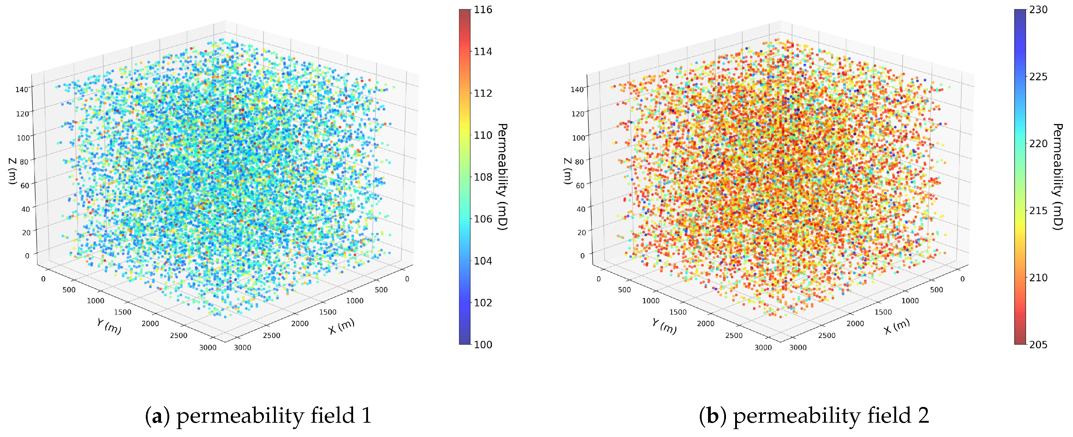
Figure 2.
Oil production rate and cumulative oil production curves over time: =100 mD.
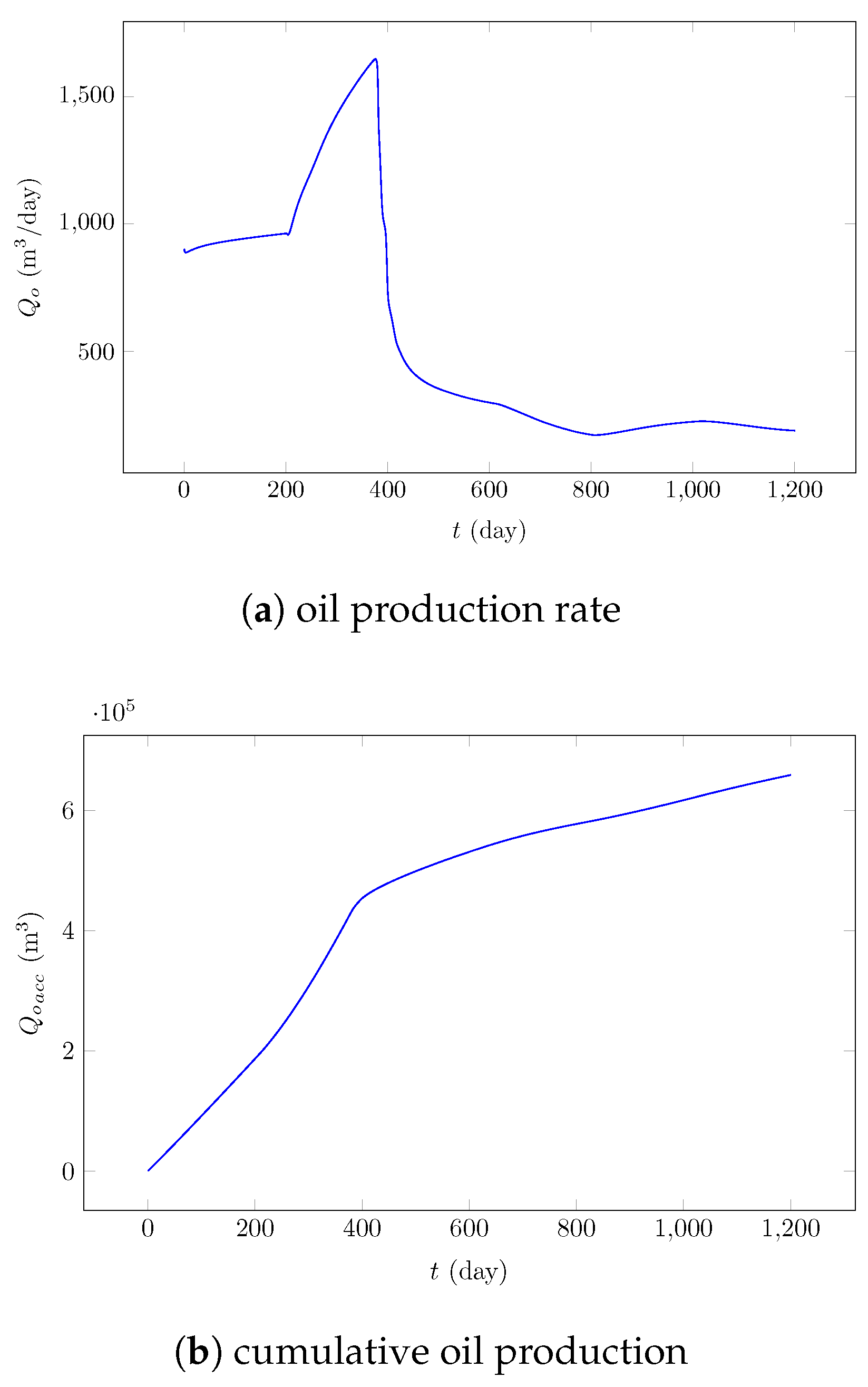
Figure 3.
Water and gas saturations as a function of time at the injector well: =100 mD.
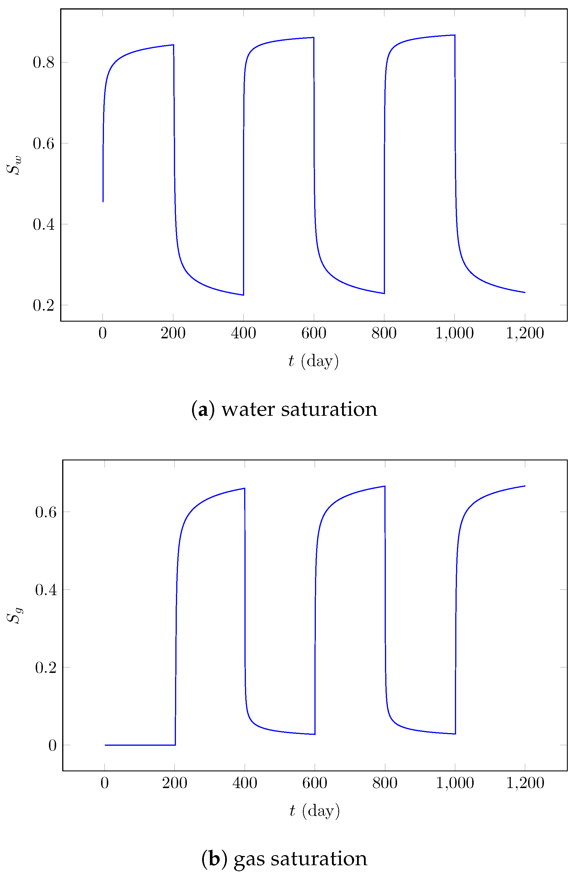
Figure 4.
Oil production rate and cumulative oil production curves over time: =200 mD.
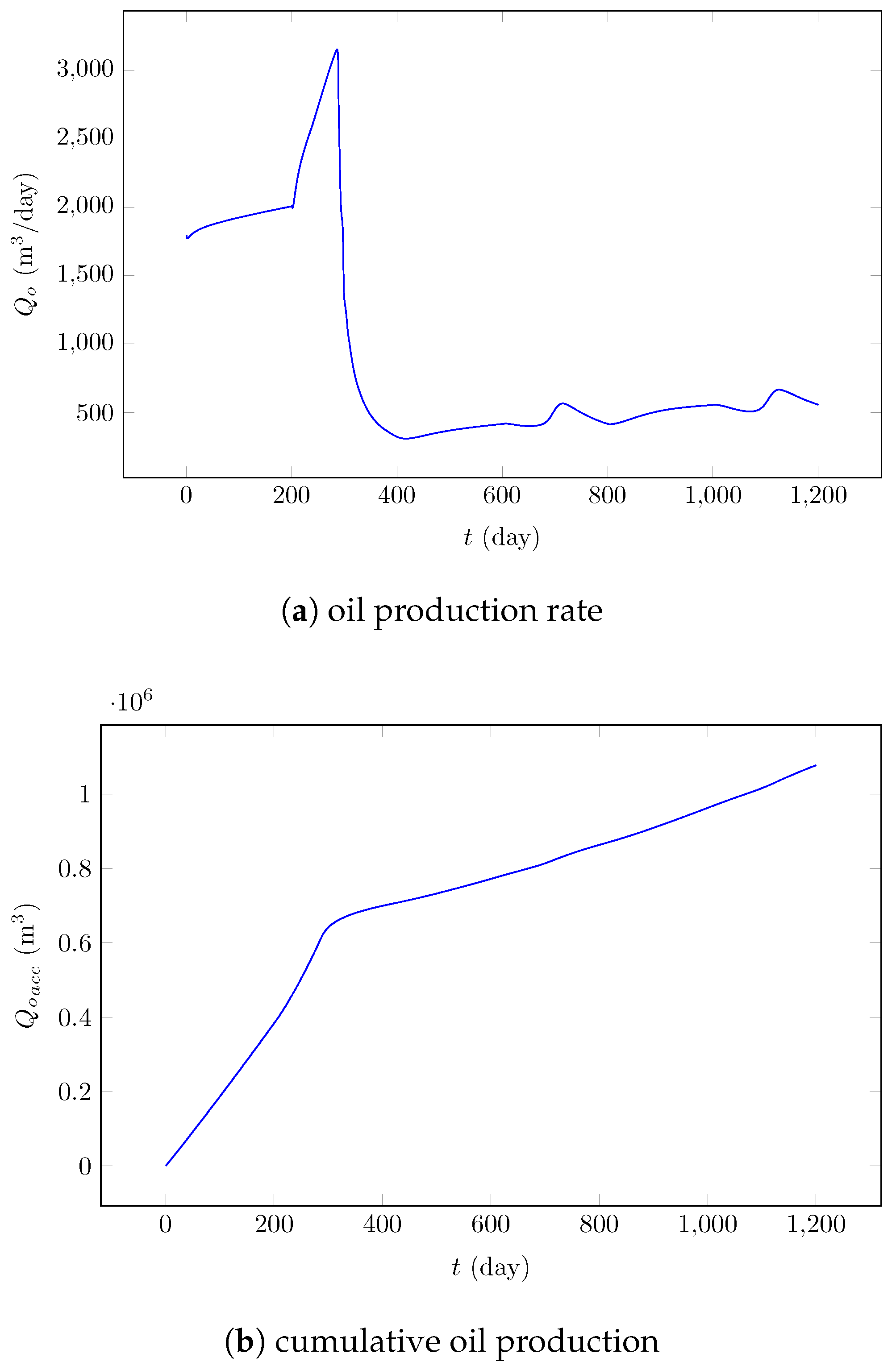
Figure 5.
Water and gas saturations as a function of time at the injector well: =200 mD.
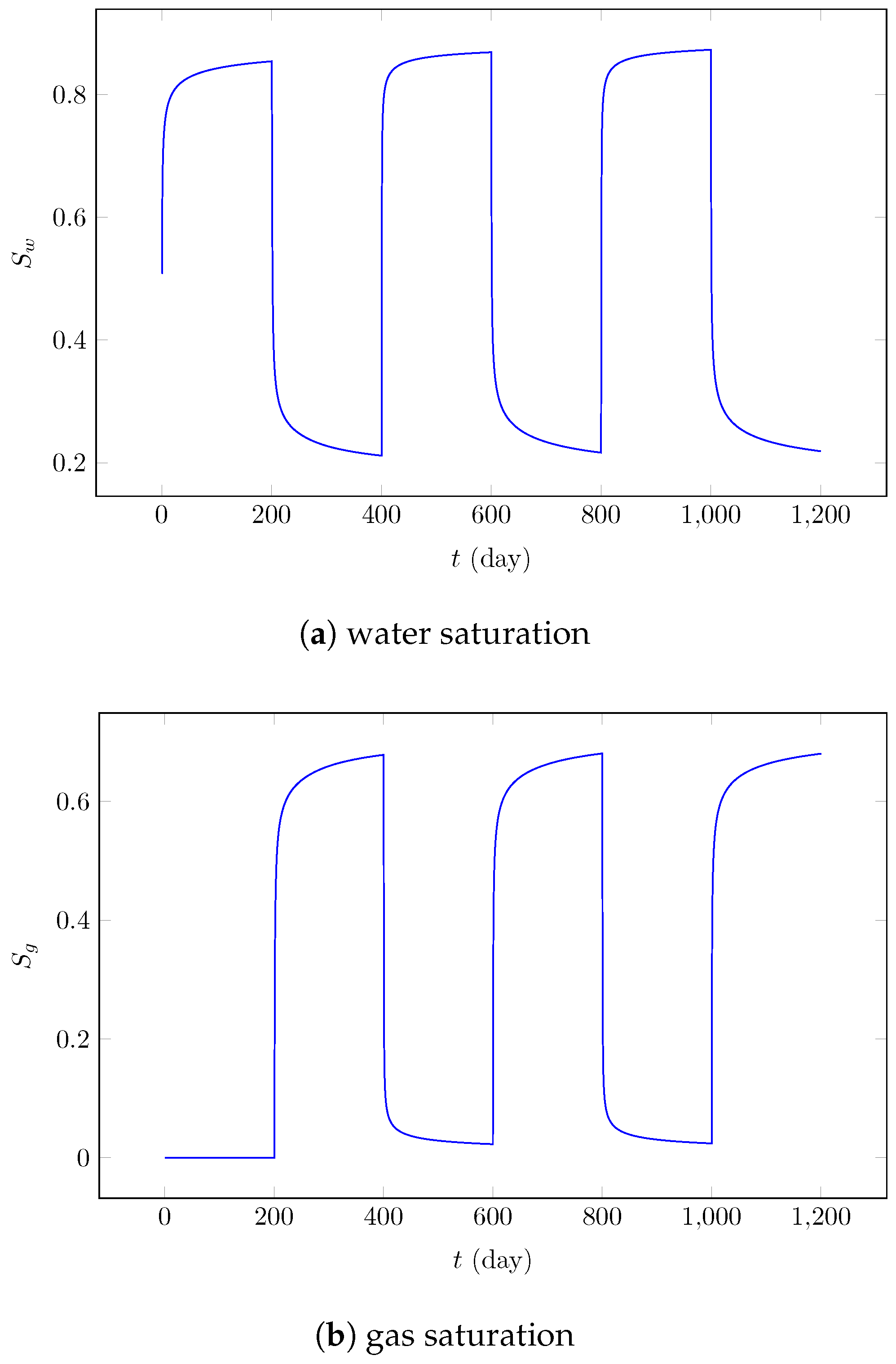

Table 1.
Parameters for FVF determination.
| Parameter | Value | Unit |
|---|---|---|
| 1.14 | – | |
| 1.01 | – | |
| 7.25 × 10⁻⁷ | kPa−1 | |
| 4.35 × 10⁻⁷ | kPa−1 | |
| 0.6 | – |
Table 2.
Parameters for rock permeability determination.
| Parameter | Value | Unit |
|---|---|---|
| 1.45 × 10⁻⁷ | kPa−1 | |
| 13789.52 | kPa | |
| 0.2 | – |
Table 3.
Relative permeability and capillary pressure determination parameters.
| Parameter | Value | Unit |
|---|---|---|
| 4 | – | |
| 2 | – | |
| 0.8 | – | |
| 0.3 | – | |
| 110.316 | kPa | |
| 68.9476 | kPa | |
| 0.15 | – | |
| 0.0 | – | |
| 0.10 | – |
Table 4.
Domain dimensions for heterogeneous permeability field generation.
| Parameter | Value | Unit |
|---|---|---|
| 3000.0 | m | |
| 150.0 | m | |
| 200 | – | |
| 30 | – |
Table 5.
Statistical parameters for heterogeneous permeability field generation.
| Parameter | Field 1 | Field 2 | Unit |
|---|---|---|---|
| 100 | 200 | mD | |
| 85 | 170 | mD | |
| 115 | 230 | mD | |
| 5 | 10 | mD |
Table 6.
Variogram parameters for heterogeneous permeability field generation.
| Parameter | Value | Unit |
|---|---|---|
| 0.2 | – | |
| 0.8 | – | |
| 1125.0 | m | |
| 1125.0 | m | |
| 100.0 | m |
Table 7.
General simulation parameters for three-phase flow.
| Parameter | Value | Unit |
|---|---|---|
| g | 9.81 | m/s2 |
| 12065.83 | kPa | |
| 13789.52 | kPa | |
| 27579.04 | kPa | |
| 55158.08 | kPa | |
| 20684.28 | kPa | |
| T | 338.71 | K |
Disclaimer/Publisher’s Note: The statements, opinions and data contained in all publications are solely those of the individual author(s) and contributor(s) and not of MDPI and/or the editor(s). MDPI and/or the editor(s) disclaim responsibility for any injury to people or property resulting from any ideas, methods, instructions or products referred to in the content. |
© 2025 by the authors. Licensee MDPI, Basel, Switzerland. This article is an open access article distributed under the terms and conditions of the Creative Commons Attribution (CC BY) license (http://creativecommons.org/licenses/by/4.0/).
Copyright: This open access article is published under a Creative Commons CC BY 4.0 license, which permit the free download, distribution, and reuse, provided that the author and preprint are cited in any reuse.


