
Submitted:
29 October 2025
Posted:
10 November 2025
You are already at the latest version
Abstract
Aiming at the estimation efficiency problem of multicollinearity and longitudinal data correlation in the varying coefficient partially nonlinear models, a method based on QR decomposition and quadratic inference function (QIF) is proposed to obtain the orthogonality estimation of parameter components and varying coefficient functions. QR decomposition eliminates the pathology of the design matrix, and combines the adaptive weighting of the relevant structures within the group by QIF to effectively capture the complex correlation structure of longitudinal data. The theoretical analysis proves the asymptotic nature of the estimator, and the efficiency of the estimation method proposed in this paper is verified by simulation experiments.
Keywords:
varying coefficient partially nonlinear model
; longitudinal data
; QR decomposition
; quadratic inference function
MSC: 62G05; 62G20
1. Introduction
In recent years, longitudinal data have attracted much attention due to their wide applications in fields such as biomedicine, economics and social sciences. This type of data is obtained through repeated observations of the same subject at different time points. As a result, multiple measurement results of the same subject exhibit temporal or spatial dependence, which makes the traditional independent and identically distributed assumption no longer applicable. To address this issue, the varying coefficient partially nonlinear model has become one of the research hotspots, as it combines the interpretability of parametric models and the flexibility of nonparametric models. Li and Mei [1] put forward a profile nonlinear least squares estimation approach to estimate the parameter vector and coefficient function vector of the varying coefficient partially nonlinear model, and further derived the asymptotic characteristics of the obtained estimators.
Important progress has been made in model estimation in existing studies. Yu and Zhu et al. [2] constructed robust estimators for the partially linear additive model under functional data. Yan and Tan et al. [3] explored the empirical likelihood inference targeting the partially linear errors-in-variables model under longitudinal data. Varying coefficient partially nonlinear model based on mode regression, a robust two-stage method for estimation and variable selection was proposed by Xiao and Liang [4]. Zhao and Zhou et al. [5] put forward a new orthogonality-based empirical likelihood inference method through orthogonal estimation techniques and empirical likelihood inference methods, which is used to estimate the parametric and nonparametric components in a class of varying coefficient partially linear instrumental variable models for longitudinal data. Liang and Zeger [6] applied the generalized estimating equation to longitudinal data analysis, which effectively handles the correlation issue of longitudinal data. For the varying coefficient partially nonlinear quantile regression model under randomly left-censored data, Xu and Fan et al. [7] introduced a three-stage estimation weighting method.
However, significant challenges still exist in the existing methods for estimating the varying coefficient partially nonlinear model. For instance, the estimation of nonlinear parameters is easily disturbed by nonparametric components and longitudinal correlation structures, leading to reduced estimation efficiency; when there is multicollinearity among explanatory variables, the ill-posed nature of the design matrix will further decrease the stability of estimation. Such issues severely limit the performance and practicality of the model in practical applications.
To address the above issues, existing studies have proposed a variety of improved methods. For example, Qu and Lindsay et al. [8] used the quadratic inference function to improve the estimating equation, and this method maintains optimal performance even when the working correlation structure is misspecified. Bai and Fung et al. [9] applied the quadratic inference function to handle longitudinal data, and the results demonstrate that the proposed estimation method exhibits excellent asymptotic properties. Schumaker [10] used B-spline basis functions to approximate the varying coefficient part, which improves the computational efficiency. Wei and Wang et al. [11] proposed a model averaging method for linear models with randomly missing response variables. Jiang and Ji et al. [12] proposed an estimation method for the varying coefficient partially nonlinear model based on the exponential squared loss function. Xiao and Chen [13] proposed a procedure for local bias-corrected cross-sectional nonlinear least squares estimation. For left-censored data, Xu and Fan et al. [14] established a quantile regression estimation and variable selection method for the varying coefficient partially nonlinear model. Based on the varying coefficient partially nonlinear model where the nonparametric part has measurement errors, Qian and Huang [15] discussed a modified profile least squares estimation method. Wang and Zhao et al. [16] proposed an inverse probability weighted cross-sectional least squares method to estimate unknown parameters and nonparametric functions for the varying coefficient partially nonlinear model.
This paper proposes an orthogonal estimation framework that integrates QR decomposition and the QIF. QR decomposition can effectively eliminates the ill-posed nature of the design matrix and improves numerical stability. The QIF method avoids the limitations of traditional generalized estimating equations by adaptively weighting the intra-group correlation structure, significantly enhancing estimation efficiency. This study not only provides a new theoretical tool for longitudinal data analysis but also offers a feasible solution to complex modeling problems in practical applications.
The structure of this paper is arranged as follows: Section 2 introduces the model specification and estimation method, including the specific implementation of QR decomposition and QIF; Section 3 discusses the asymptotic properties of the estimators; Section 4 verifies the superiority of the proposed method through simulation experiments; The proof process of the main conclusions is provided in the Appendix.
2. Models and Methods
Consider the varying coefficient partially nonlinear model introduced by Li and Mei [1]:
where, is the response variable, , , and are covariates, and are unknown smooth functions, is a nonlinear function with a known form, denotes a q-dimensional unknown parameter vector, and is the model error with mean zero and variance .
2.1. Estimation of Parameter Vector
Considering the model (1) under longitudinal data, suppose the j-th observation of the i-th individual satisfies:
among them, has a mean of zero, and are covariates.
Based on the idea of Schumaker [10], the unknown function can be approximated using basis functions. The B-spline basis functions are denoted by the vector . The dimension L is defined as , where K and M represent the number of interior knots and the order of the spline, respectively. Then can be approximately expressed as
here are the coefficient vector for the B-spline basis functions. model (2) can be expressed as
define , where ⊗ is the Kronecker product, and let , , , , . Then model (4) can be expressed as
Suppose that for all , the matrices have full column rank, their QR decomposition can be expressed as:
where is an orthogonal matrix, is a triangular matrix, and denotes a zero matrix. The matrix can be divided into two parts as , where is a matrix and is a matrix. Substitute the decomposition of into (6) to obtain , from the properties of orthogonal matrices, can be derived, and then is obtained. Multiplying both sides of Equation (5) by , and we get:
It is easy to see that model (7) is a regression model containing only unknown parameters. Following Liang [6], the generalized estimating equation for can be defined as:
among them, , , is the covariance matrices of , and the structure of can also be expressed as according to the method of Liang [6], where is a diagonal matrix, is a working correlation matrix, and is a correlation parameter. Since a consistent estimator of is not always available in practice, we adopt the QIF method to approximate the working correlation matrix through a set of basis matrices, thereby avoiding direct specification of the correlation structure. Let be a set of basis matrices and be coefficients satisfying:
Define the extended score function as follows:
Thus, the QIF for can be defined as:
where , in this case, the estimator of is obtained by minimizing the objective function :
2.2. Estimation of the Coefficient Functions
The QIF effectively handles the correlation in longitudinal data and improves estimation efficiency by constructing a set of estimating equations. Therefore, after obtaining the initial estimates of the parameters , we also use the QIF method to estimate the coefficient functions
Substitute the estimator of into Equation (5), resulting in:
where , assuming that the covariance matrix of is , and its structure is expressed following Liang [6] as , where is a diagonal matrix, is a working correlation matrix, and is a correlation parameter. Assuming is known, construct the following estimating equation:
In practical applications, is usually unknown. Based on this, we still adopt the QIF method and use to approximate , then we have:
Define the extended score function as follows:
Thus, the QIF for can be defined as:
where . In this case, the estimate of can be obtained by minimizing the objective function :
Thus, the estimate of the coefficient function can be expressed as:
where is the component corresponding to the k-th coefficient function in .
3. Main Conclusions
This section studies the asymptotic properties of the estimators and , assuming that and are the true values of and respectively, is the true value of , and and are the k-th components of and respectively. First, we present some common regularity conditions in longitudinal data analysis:
(C1) The random variable U has a bounded support , and its probability density function is positive and has continuous second-order derivatives.
(C2) The varying coefficient function is continuously differentiable of order r on , where .
(C3) For any Z, is continuous with respect to , and has continuous partial derivatives of order r.
(C4) holds, and there exists some satisfying .
(C5) The covariates and are assumed to satisfy the following conditions: , ,
(C6) Let be interior nodes on . Furthermore, let then there exists a constant such that:
(C7) Define , then we have:
Among them, and are constant matrices, and denotes convergence in probability. Define and , additionally, assume that and are both invertible.
It is noted that, conditions (C1) to (C5) are common conditions in varying coefficient partially nonlinear models components, Condition (C6) indicates that is a uniform partition sequence over the interval , and Condition (C7) is used for subsequent proofs.
Theorem 1.
Under conditions (C1) to (C7), and when , it follows that:
where the matrix , denotes convergence in distribution.
Theorem 2.
Under conditions (C1) to (C7), the number of nodes , and when , it follows that:
where denotes the norm of the function.
4. Simulation Study
This section evaluates the finite-sample performance of the proposed orthogonality estimation method based on QR decomposition and quadratic inference functions in varying coefficient partially nonlinear models through a Monte Carlo simulation study. Consider the following model:
among them, the covariates both follow normal distributions, the nonlinear function is defined as , with the parameter vector . Additionally, , the coefficient function , the error term follows an AR(1) process, and its structure is: , where to ensure the error variance is 0.5.
The sample size is set to , for the i-th subject, the number of repeated measurements is , and 1000 simulation runs are conducted for each case. The method combining QR decomposition and QIF proposed in this paper (OQIF) is compared with the profile nonlinear least squares method (PNLS) proposed by Li and Mei [1]. After sorting out, the following Table 1 and Table 2 are obtained.
It can be seen from the results in Table 1 that as the sample size increases, the bias and standard deviation of both methods decrease. However, the bias and standard deviation of the OQIF method are smaller, indicating more accurate estimation. Although a larger sample size improves the estimation accuracy of both methods, the OQIF method performs better in bias control.
The results in Table 2 show that the average length of the confidence interval of the OQIF method is significantly shorter than that of the PNLS method, demonstrating higher estimation efficiency, the coverage rate of the OQIF method is closer to the ideal 95%, while although the coverage rate of the PNLS method has improved, it is still below 95%.
In conclusion, when the sample size increases from 100 to 200, the OQIF method demonstrates higher estimation accuracy and stronger robustness across all evaluation indicators. These trend analyses further confirm the theoretical advantages and practical application value of the OQIF method in handling nonlinear longitudinal data.
We further conducted 1000 simulations and plotted boxplots of the 1000 RMSE values for parameters and , as shown in Figure 1 and Figure 2. From the figures, we can observe the following: the RMSE values of and for both methods decrease as the sample size increases, however, the OQIF method already exhibits good performance with a small sample size (n=100), while the PNLS method requires a larger sample size to achieve similar accuracy. The boxplots of the OQIF method are more symmetric and compact, indicating that the distribution of its estimators is closer to the normal distribution and has better statistical properties. Additionally, the OQIF method has significantly fewer outliers than the PNLS method, demonstrating stronger robustness against abnormal data. This suggests that the overall performance of the OQIF method in parameter estimation is superior to that of the PNLS method, with more pronounced advantages especially in cases of finite samples.
Next, we estimate the coefficient function , simulate 1000 times and draw the box plot of the RMSE of under different samples, resulting in Figure 3 below.
As can be seen from the above boxplots: with the increase in sample size, the error distributions of both the OQIF method and the PNLS method become more concentrated, but the error of the OQIF method is significantly smaller than that of the PNLS method. This further verifies the superiority of the OQIF method in the varying coefficient partially nonlinear model.
Author Contributions
Conceptualization, J.G., X.Z. and C.W.; methodology, J.G., X.Z. and C.W.; software, J.G, and C.W.; validation, J.G., X.Z. and C.W.; data curation, J.G. and X.Z.; writing—original draft preparation, J.G.; writing—review and editing, X.Z.; funding acquisition, X.Z. All authors have read and agreed to the published version of the manuscript.
Funding
This research was funded by the Natural Science Foundation of Shandong Province (Grant No.ZR2022MA065).
Data Availability Statement
The original contributions presented in this study are included in the article. Further inquiries can be directed to the corresponding author.
Conflicts of Interest
The authors declare no conflicts of interest.
Abbreviations
The following abbreviations are used in this manuscript:
| QIF | Quadratic inference function |
| OQIF | The combination of QR decomposition and QIF |
| PNLS | Profile nonlinear least squares |
Appendix A
To prove Theorems 1 and 2, we first present the following lemmas:
Lemma A1.
Let c be a positive constant, and let , be a sequence of independent and identically distributed random variables. If it satisfies conditions and , then we have .
Proof.
The result has been proven in Lemma A.2 of Zhao and Xue [17]. □
Lemma A2.
Assume that the conditions (C1) to (C7) hold, when , we have:
where is defined in Condition (C7).
Proof.
Let , , , combining with , we can obtain:
Let denote the k-th component of , combining with Equation (11), we obtain:
Conclusion can be derived from Conditions (C2), (C5), and Corollary 6.21 of Schumaker [10], further combining with Lemma A1, we obtain:
Let , combining with and , we can thus conclude and , where is defined in Condition (C7). We further let , it follows that and
where combining with Condition (C7) and the Law of Large Numbers, we conclude that:
Furthermore, for any constant vector that satisfying condition , we have and , where C is a positive constant. Therefore, satisfies the Lyapunov condition of the Central Limit Theorem. Thus, we obtain: Further combining with Equations (A4) and (A5), we can obtain:
The proof of Lemma A2 is completed. □
Lemma A3.
Assume that the conditions (C1) to (C7) hold, we have and , where and are defined in Condition (C7), and is the first-order derivative of with respect to .
Proof.
After simple calculations, we obtain:
Combining with Condition (C7) and the Law of Large Numbers, we have that:
Further combining with Equation (A8), we obtain: . The proof of Lemma 2 shows that:
Similar to the proof of Equation (A5), we can obtain:
Therefore, , The proof of Lemma 3 is completed. □
Lemma A4.
Assume that the conditions (C1) to (C7) hold, we obtain:
and
Where and are the first-order derivative and the second-order derivative of , respectively.
Proof.
According to the definition of , we can obtain the following result through calculation:
It follows from Lemma A2 that: . Further, from Condition (C7) and Lemma A3, we can obtain:
Similarly, we can obtain the following through calculation:
where,
Combining Lemma A2 and Lemma A3, we can obtain the following: and are both , while and are both , thus, . The proof of Lemma A4 is completed. □
Proof of Theorem 1.
Noting that , thus , according to the Lagrange Mean Value Theorem, we have:
where lies between and , thus, we have:
Combining Lemma A3 and Lemma A4, we can obtain:
and
Proof of Theorem 2.
Let . That is, we need to prove that for any given , there exists a constant C such that the following holds:
Let . By Taylor’s Formula, we can obtain:
where lies between and . Noting that , we can obtain the following through the assumption conditions and some calculations: , , . Thus, there exists a sufficiently large constant C such that when , can control and ; therefore, Equation (A8) holds, and there further exists a maximum point satisfying:
then we can obtain:
The proof of Theorem 2 is completed. □
References
- Li, T.; Mei, C. Estimation and inference for varying coefficient partially nonlinear models. Journal of Statistical Planning and Inference 2013, 143, 2023–2037. [Google Scholar] [CrossRef]
- Yu, P.; Zhu, Z.; Shi, J.; Ai, X. Robust estimation for partial functional linear regression model based on modal regression. Journal of Systems Science and Complexity 2020, 33, 527–544. [Google Scholar] [CrossRef]
- Yan, L.; Tan, X.y.; Chen, X. Empirical likelihood for partially linear errors-in-variables models with longitudinal data. Acta Mathematicae Applicatae Sinica, English Series 2022, 38, 664–683. [Google Scholar] [CrossRef]
- Xiao, Y.; Liang, L. Robust estimation and variable selection for varying-coefficient partially nonlinear models based on modal regression. Journal of the Korean Statistical Society 2022, 51, 692–715. [Google Scholar] [CrossRef]
- Zhao, P.; Zhou, X.; Wang, X.; Huang, X. A new orthogonality empirical likelihood for varying coefficient partially linear instrumental variable models with longitudinal data. Communications in Statistics-Simulation and Computation 2020, 49, 3328–3344. [Google Scholar] [CrossRef]
- Liang, K.Y.; Zeger, S.L. Longitudinal data analysis using generalized linear models. Biometrika 1986, 73, 13–22. [Google Scholar] [CrossRef]
- Xu, H.X.; Fan, G.L.; Liang, H.Y. Quantile regression for varying-coefficient partially nonlinear models with randomly truncated data. Statistical Papers 2024, 65, 2567–2604. [Google Scholar] [CrossRef]
- Qu, A.; Lindsay, B.G.; Li, B. Improving generalised estimating equations using quadratic inference functions. Biometrika 2000, 87, 823–836. [Google Scholar] [CrossRef]
- Bai, Y.; Fung, W.K.; Zhu, Z.Y. Penalized quadratic inference functions for single-index models with longitudinal data. Journal of Multivariate Analysis 2009, 100, 152–161. [Google Scholar] [CrossRef]
- Schumaker, L. Spline Functions: Basic Theory. Wiley 1981. [Google Scholar]
- Wei, Y.; Wang, Q.; Liu, W. Model averaging for linear models with responses missing at random. Annals of the Institute of Statistical Mathematics 2021, 73, 535–553. [Google Scholar] [CrossRef]
- Jiang, Y.; Ji, Q.; Xie, B. Robust estimation for the varying coefficient partially nonlinear models. Journal of Computational and Applied Mathematics 2017, 326, 31–43. [Google Scholar] [CrossRef]
- Xiao, Y.T.; Chen, Z.S. Bias-corrected estimations in varying-coefficient partially nonlinear models with measurement error in the nonparametric part. Journal of Applied Statistics 2018, 45, 586–603. [Google Scholar] [CrossRef]
- Xu, H.X.; Fan, G.L.; Liang, H.Y. Quantile regression for varying-coefficient partially nonlinear models with randomly truncated data. Statistical Papers 2024, 65, 2567–2604. [Google Scholar] [CrossRef]
- Qian, Y.; Huang, Z. Statistical inference for a varying-coefficient partially nonlinear model with measurement errors. Statistical Methodology 2016, 32, 122–130. [Google Scholar] [CrossRef]
- Wang, X.; Zhao, P.; Du, H. Statistical inferences for varying coefficient partially non linear model with missing covariates. Communications in Statistics-Theory and Methods 2021, 50, 2599–2618. [Google Scholar] [CrossRef]
- Zhao, P.; Xue, L. Empirical likelihood inferences for semiparametric varying-coefficient partially linear errors-in-variables models with longitudinal data. Journal of Nonparametric Statistics 2009, 21, 907–923. [Google Scholar] [CrossRef]
Figure 1.
Box plot of 1000 RMSE values for under the OQIF (A) and PNLS (B) methods
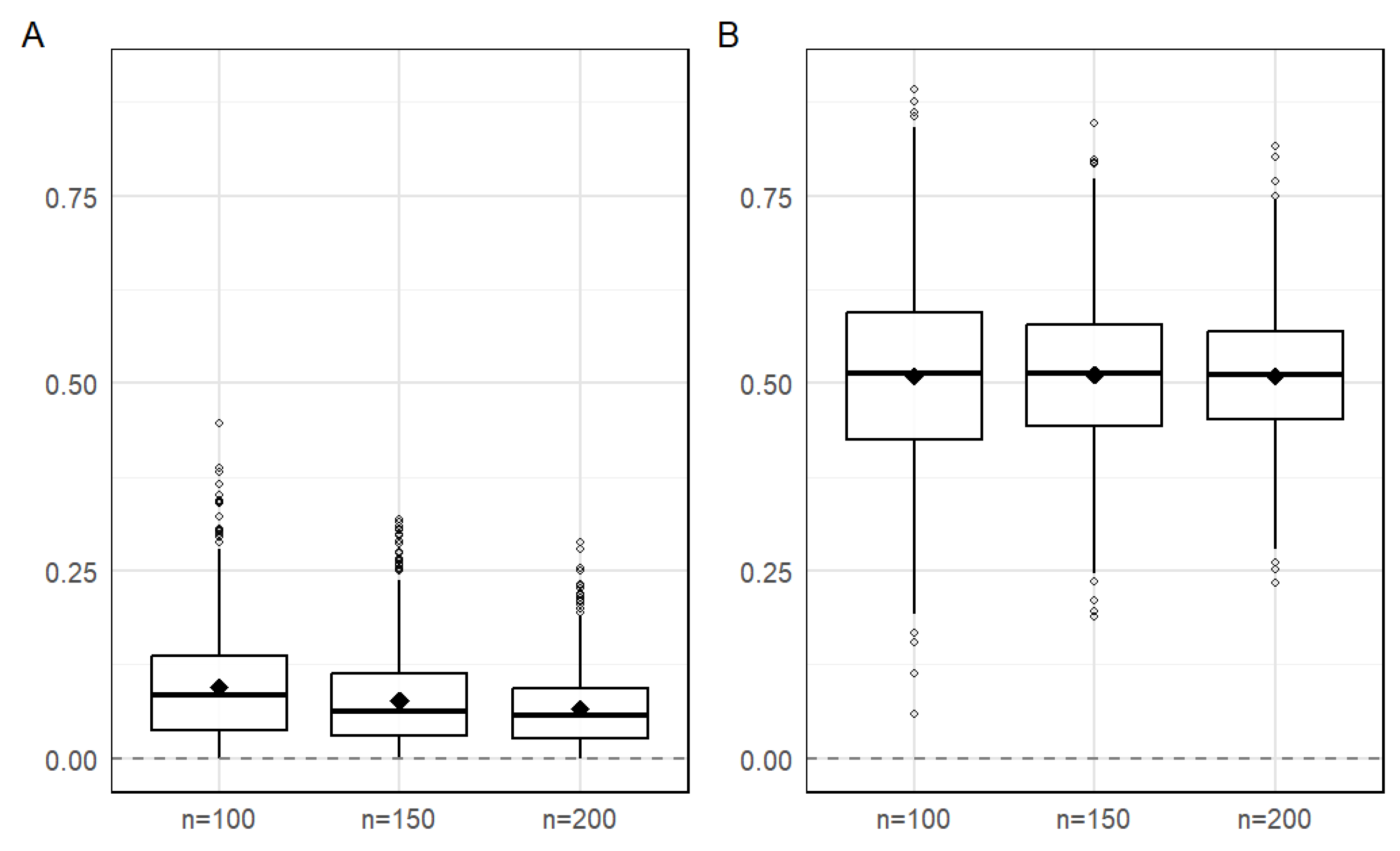
Figure 2.
Box plot of 1000 RMSE values for under the OQIF (A) and PNLS (B) methods
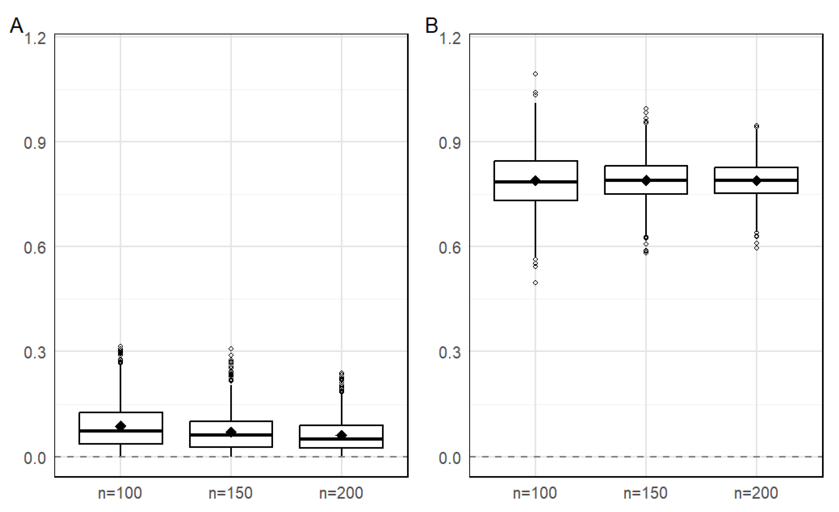
Figure 3.
Box plot of 1000 RMSE for with different sample sizes
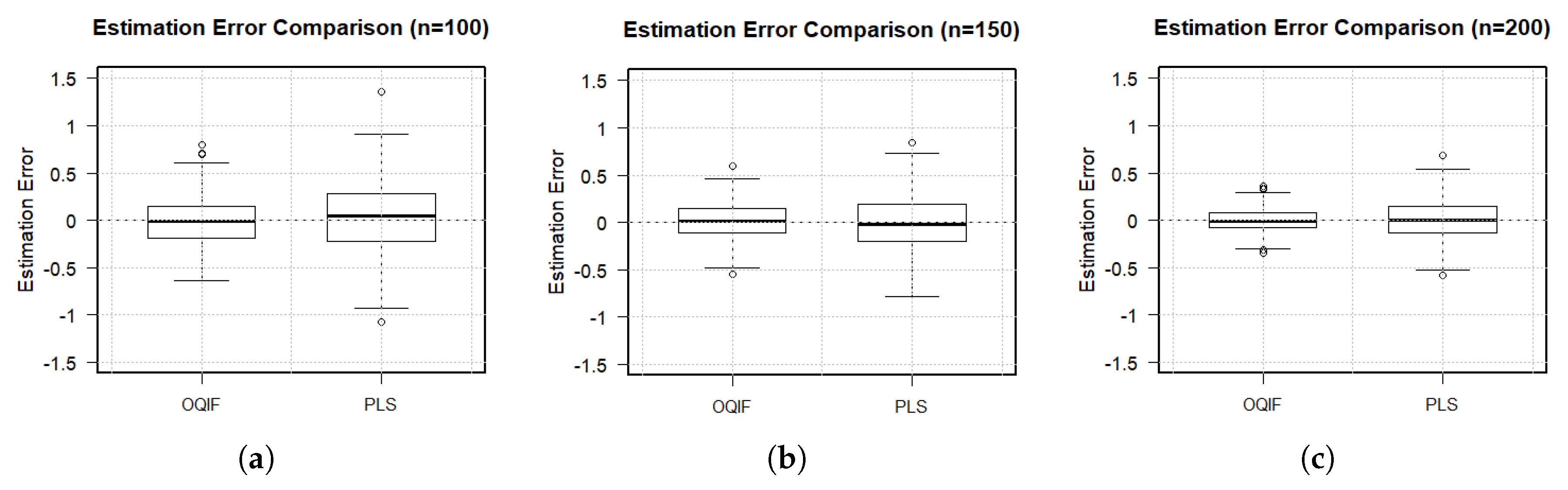

Table 1.
The bias and standard deviation of and measured by different methods
| Method | Parameter | ||||||
|---|---|---|---|---|---|---|---|
| Bias | SD | Bias | SD | Bias | SD | ||
| OQIF | 0.00257 | 0.02012 | 0.00123 | 0.01890 | 0.00079 | 0.01568 | |
| -0.00390 | 0.03890 | -0.00235 | 0.03568 | -0.00157 | 0.02946 | ||
| PNLS | 0.01457 | 0.03012 | 0.01235 | 0.02789 | 0.00988 | 0.02346 | |
| -0.02789 | 0.05890 | -0.02457 | 0.05235 | -0.02012 | 0.04457 | ||
Table 2.
Confidence Interval Length and Coverage Probability Comparison
| Method | Parameter | n=100 | n=150 | n=200 | |||
|---|---|---|---|---|---|---|---|
| Length | Coverage | Length | Coverage | Length | Coverage | ||
| OQIF | 0.07671 | 0.943 | 0.07190 | 0.947 | 0.05971 | 0.951 | |
| 0.14853 | 0.937 | 0.13551 | 0.941 | 0.11329 | 0.948 | ||
| PNLS | 0.11329 | 0.911 | 0.10065 | 0.918 | 0.08541 | 0.925 | |
| 0.20995 | 0.899 | 0.18773 | 0.905 | 0.15946 | 0.912 | ||
Disclaimer/Publisher’s Note: The statements, opinions and data contained in all publications are solely those of the individual author(s) and contributor(s) and not of MDPI and/or the editor(s). MDPI and/or the editor(s) disclaim responsibility for any injury to people or property resulting from any ideas, methods, instructions or products referred to in the content. |
© 2025 by the authors. Licensee MDPI, Basel, Switzerland. This article is an open access article distributed under the terms and conditions of the Creative Commons Attribution (CC BY) license (http://creativecommons.org/licenses/by/4.0/).
Copyright: This open access article is published under a Creative Commons CC BY 4.0 license, which permit the free download, distribution, and reuse, provided that the author and preprint are cited in any reuse.


