
Submitted:
06 November 2025
Posted:
07 November 2025
You are already at the latest version
Abstract
The amount of millimeter-wave radiation which is absorbed or transmitted through pig skin is investigated. Millimeter waves are currently used in a range of technologies, including communication systems, fog-penetrating radar, and the detection of hidden weapons or drugs. They have also been proposed for use in non-lethal weaponry and, more recently, in targeted cancer therapies. Since pigs are often used as biological models for humans, determining how deeply millimeter waves penetrate a pig’s skin and influence the underlying tissues is essential for understanding their potential effects on humans. This experimental study aims to quantify that penetration and associated energy loss.
Keywords:
millimeter waves
; cancer therapy
; non-ionizing radiation
; physical properties of biological tissue
1. Introduction
Cancer remains one of the deadliest diseases known to humanity, with lung cancer being the leading cause of cancer-related deaths. It is often diagnosed at an advanced and untreatable stage [1,2]. While standard chemotherapy can be effective against certain cancers, its success is limited for many types, offering only modest improvements in survival [3]. Lung cancer mortality is mainly due to metastasis, a complex multi-step process, and the survival rate without treatment is extremely poor—about 98% [3]. Despite extensive research, effective methods for early detection and treatment of lung cancer are still lacking.
The interaction between electromagnetic (EM) waves and biological cells has been studied for several decades [4,5]. Non-thermal effects of EM radiation have been examined in various biological systems, including bacteria, mammalian cell cultures, and living organisms [6,7,8]. Although much research has been devoted to this topic, and several reviews have attempted to clarify the mechanisms behind non-thermal interactions, a consistent theoretical and experimental framework has yet to be achieved [9,10].
In vitro studies have shown that millimeter waves in the 75–110 GHz frequency range (wavelengths of 2.73–4 mm) can selectively destroy H1299 lung cancer cells while leaving healthy cells (MCF-10A breast epithelial cells) unharmed, even at very low power levels. This selectivity has been confirmed to be non-thermal in nature [11,12,19,20,21]. The next logical step is to determine whether this selective effect also occurs in living organisms.
Animals such as pigs and mice are commonly used as biological models for humans. Many medical treatments and drugs, including cancer therapies, are first tested on pigs and mice to evaluate their safety and effectiveness. In such experiments, human tumors are implanted under the mouse or pig’s skin and monitored over time. A thermal treatment of mice using millimeter waves was described in [4], where a gyrotron was employed to heat malignant tumors with sub-terahertz radiation. The results showed a gradual reduction in tumor volume leading to complete disappearance.
More advanced studies have combined hyperthermia with photodynamic therapy (PDT), using specialized photosensitizers, yielding even better outcomes. While hyperthermia alone sometimes allows tumor regrowth, the combined therapy prevents it entirely. Another variation involves preheating the tumor below hyperthermic levels (below 43 °C) with millimeter waves before applying PDT, which significantly enhances treatment efficiency.
Regardless of whether the underlying therapeutic mechanism is thermal or non-thermal, understanding how deeply millimeter-wave energy penetrates tissue is crucial, as this determines the actual energy delivered to the tumor. Therefore, measuring the power loss as millimeter waves pass through mouse skin is essential.
Mouse and Pig models will also be used in our future experiments, repeating and extending the studies in [11,12]. However, these models are only meaningful if the extent of wave penetration through the skin is well understood. The goal of the present work is thus to provide accurate experimental measurements of millimeter-wave transmission loss through a pig’s skin. Although our primary motivation is related to lung cancer treatment, the results are broadly relevant to modeling other human cancers or tissues grown in immunodeficient mice, as well as to studies involving non-lethal directed-energy applications [13].
The paper is organized as follows: first the experimental setup is described, followed by the results and their interpretation, and finally present the conclusions and implications for future studies.
2. Materials and Methods
The experimental plan
The purpose of the experiment is to investigate the degree of attenuation of electromagnetic radiation at microwave frequencies in animal skin. Figure 1 and Figure 2 below describe the experimental setup.
The measurements were performed using a network analyzer at frequencies of 75-110 GHz.
The range between the receiving and transmitting antennas and the position of the sample is controllable and was placed on a dedicated rail for measurements at different distances. In addition, in the constructed setup the sample can be moved in a plane perpendicular to the rail for measurements at different points on the skin.
The sample is mounted inside a circular Petri dish with a diameter of 85 mm. The sample can be rotated 360 degrees inside the fixture in a plane perpendicular to the rail.
Preliminary preparations
The samples were prepared prior to the measurements. They were cut from a large skin sample. The round samples were cut with scissors and kept refrigerated at 0 degrees in bags until the day of the measurements, for about a week.
The samples were placed in separate Petri dishes, so that the sample would cover the entire surface of the dish. Each dish was marked with a marker for rotation position 0 - defined by the biologists in our group, according to the structure of the skin, that is with the direction of hair growth.
On a Petri dish, three measurement points in the near field were marked so that they would be aligned with the "0" angle axis (see Figure 3).
Array for near-field measurements
The sample (Petri dish) was placed in the radiation near-field domain. This domain is defined to be in the range between the Reactive near field and the Far field. According to Fraunhofer distance:
where is the largest dimension of the antenna (for a rectangular antenna this is the diagonal):
According to the dimensions described in Figure 4 and Figure 5, the required size can be calculated:
is the wavelength. Therefore, the data presented in Table 1 follows:
Therefore, it was decided to place the samples at a distance of approximately 200 mm from the antenna.
Design of the array for far-field measurements
For far-field measurements, it is necessary to ensure that the calculated beam cross-section covers the Petri dish area. For a horn antenna with two different dimensions, one can calculate the approximate angular beam width based on the relevant diameter:
For example, for f=75GHz:
Therefore, the size of the spot reaching the sample in the far field will be calculated based on the distance at the far field boundary:
Figure 6.
Calculation of spot size on the sample at the far field boundary.
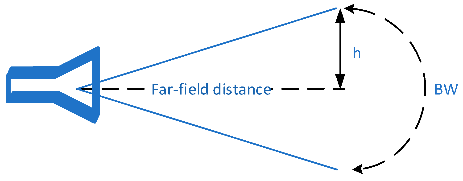
The size of the spot will be calculated according to:
Thus:

Table 2.
Beam cross-section at different frequencies versus sample size – 85 mm.
| Frequency (GHz) | Wavelength (mm) | Far field limit (mm) | Reactive near field limit (mm) |
| 75 | 4 | 477.6 | 53.27 |
| 95 | 3.158 | 605 | 59.95 |
| 110 | 2.727 | 700 | 64.51 |
According to the above data, it can be said that the size of the spot always covers the sample, assuming concentric centering of the sample.
Therefore, the samples can be placed 700 mm away from the antenna.
Due to the constraints of the experimental setup, the lengths of the cables to connect the network, measurements were performed for the near field only.
Main points of the experiment:
The experiment was carried out in two stages – preparation of the samples and measurement of basic parameters, electromagnetic measurements of S parameters, concentration, and analysis of results.
As part of the preparations for the experiment, 4 days were spent building the measurement system and placing the samples (the track and the device), 2 days of coordinating the antenna array and the network analysis, and another 3 days of preparing the samples, placing them in the Petri dish, and making measurements.
Below is the experimental plan on the day of the measurements:
Near field calibration for S21.
Calibration and measurement of S11.
Placing the fixture with the sample at the relevant location for the measurement in the antennas near field. The center of the Petri dish corresponds to the center of the beam.
Perform the measurement for each Petri dish. It is required to perform measurements for three distinct locations on the sample (which require horizontal displacement) and rotation in 90° the central position (around the axis).
S11 measurements should be performed in the near field. When measuring at each point on the Petri dish, including a 90-degree rotation. The measurements were recorded accordingly. The experiment was carried out during one day of measurements, and the results were subsequently sampled and analyzed for the purpose of compiling this report over a period of 4 weeks.
Preparation of the samples
Seven samples of pig’s skin were prepared in a round shape to fit into a Petri dish with a diameter of 85 mm. The samples were cut from a single section of skin. The separation of the skin was done in a rough manner and therefore the thickness of the skin and fat is unique to each sample. The same applies to the texture and color of the skin as depicted in Figure 7. Fourteen samples were prepared, which is twice as many as needed for the experiment (as seen in Figure 7). Of these, the seven best were selected for the measurements (based on quality of the Petri dish, level of sample retention, etc.). The samples were kept refrigerated at 0 degrees until mounted in standard Petri dishes.
On each plate with the skin specimen placed inside, a reference point 0 was defined, so that the direction of the hair in the skin (visually checked by a biologist) would correspond with the 0-180 degrees direction. In addition, a 90-degree point and three points on the horizontal axis were defined that correspond to the center and two lateral displacements of 2/3 of the diameter. These measurement points were used as a reference during the experiment – see Figure 8.
After placing the specimen on the plate, skin thickness and fat thickness were estimated at reference points for all samples. Skin thickness was similar, in the range of 1.5-3.0 mm. Fat thickness varied between samples, ranging from 3-9.5 mm. Skin color and texture differed between the different samples. It should also be noted that due to the measurement method as described in Figure 9, skin thickness was estimated only at the perimeter of the sample, so that a representative skin thickness was determined for each specimen. In practice, it is reasonable to assume that skin thickness can also vary slightly within the sample.
For the measurements, the seven samples were prepared in Petri dishes – labeled A, B, C, D, S, M, O, see Figure 10 below.
For the sake of measuring S- parameters, a dedicated measurement setup was established based on a network analyzer, associated equipment, and a pair of antennas. The setup is calibrated and coordinated to measure skin samples in a Petri dish. A dedicated mechanical device was also built that fixes the measurement geometry - including a rail on which columns with antenna fixtures were installed (in order to reduce reflections from nearby surfaces, and a column with the sample device including a screen to limit the projection area to the sample. The measurement distances and adjustment to the axes were coordinated according to the experimental plan as described at the beginning of the document (precisely controlled by the rail). In Figure 11, you can see the measurement setup, the signal generator, antenna calibration, and associated equipment.
The measurements were performed in the 70-110 GHz range, spanning 401 discrete frequencies. The array was calibrated to a baseline to eliminate the influence of the measurement array, including placing an empty Petri dish (see Figure 12 and Figure 13).
Performing measurements
During the measurement session, approximately thirty sets of measurements were performed for each sample. S21 measurements were performed at several reference points, by measuring transmission between two identical antennas, placed at various distances within a radiation field relative to the sample in the setup:
- 0-degree central position
- 90-degree central position (by rotating the Petri dish around the 0 point)
- Two laterally displaced positions by two-thirds diameter as depicted in Figure 14
S11 measurements were performed at several reference points, by attaching an antenna to the sample to obtain maximum return. The antenna is calibrated against an aluminum plate to define (reset) the baseline:
- degree central position
- 90-degree central position (by rotating the Petri dish around the 0 point)
The reflection measurements (S11) were only performed at a reference point in the center.
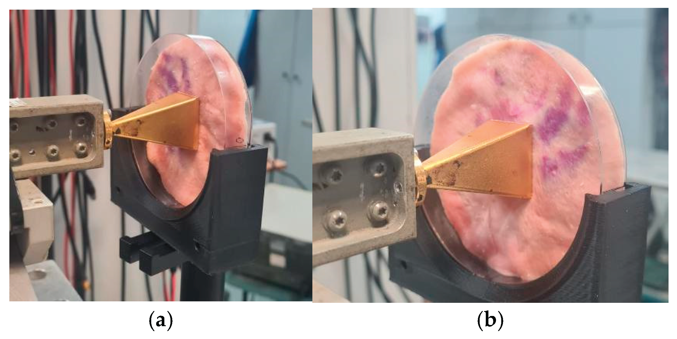
Figure 15.
Example of rotation in S11 measurement. In the right image (a) the sample can be seen in a 90-degree orientation while in the left image (b) the same sample can be seen in a 0-degree orientation.
Figure 15.
Example of rotation in S11 measurement. In the right image (a) the sample can be seen in a 90-degree orientation while in the left image (b) the same sample can be seen in a 0-degree orientation.
3. Results
Summary of results and initial data analysis
The measurement results were compiled in an Excel file that includes sheets with raw measurements of attenuation and reflection parameters (S11, S21) for each measurement. Attenuation segmentation (S21) is according to the sample thickness (for all samples are derived from a single animal skin). The results were analyzed for several representative frequencies in the studied spectrum (80, 85, 85, 90, 95, 100, 105 GHz). Absorption in animal skin was calculated for all samples across the studied spectrum. A comparative analysis of absorption in concentric measurement (the central point) was performed for all samples in 0 vs. 90 degrees orientation.
Raw S21 measurements
Figure 16.
Raw measurement S21: Measurements at the center of the sample. A – 0-degree orientation, B – 90-degree orientation. The burgundy line shows the average over the measurements along the frequency axis.
Figure 16.
Raw measurement S21: Measurements at the center of the sample. A – 0-degree orientation, B – 90-degree orientation. The burgundy line shows the average over the measurements along the frequency axis.
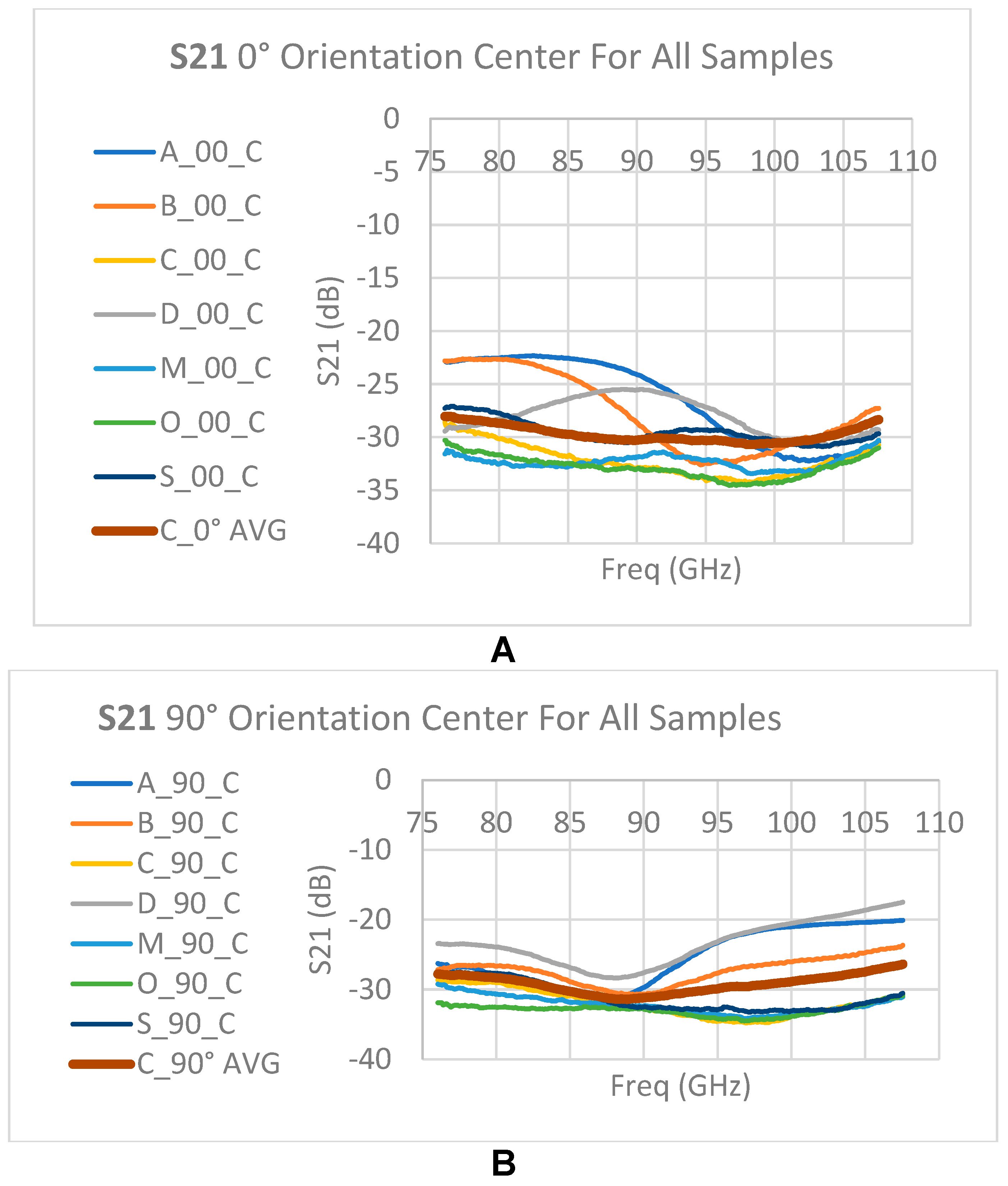
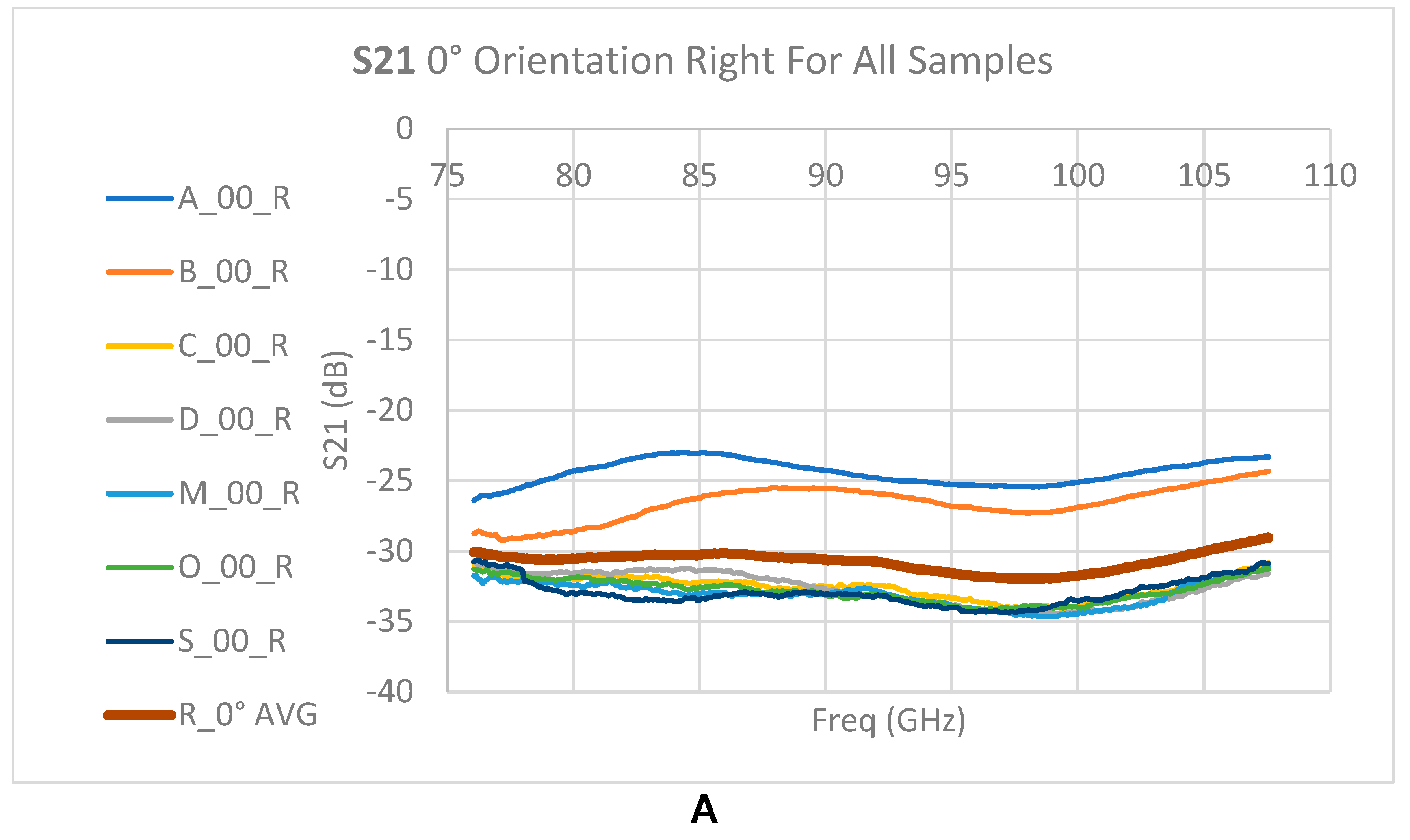
Figure 17.
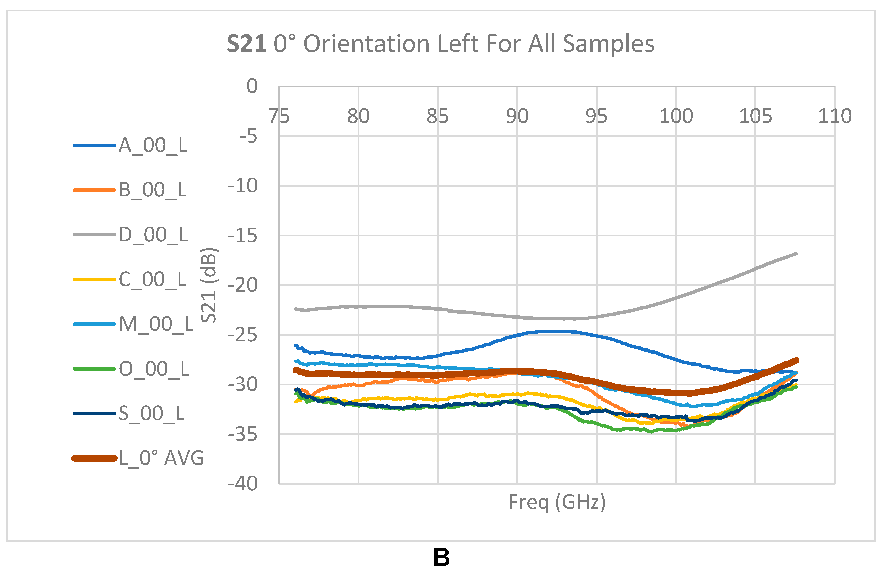
Raw measurement S21: 0-degree orientation. A - Measurements shifted to the right. B - Measurements shifted to the left. The burgundy line shows the average over the measurements along the frequency axis.
Figure 17.
Raw measurement S21: 0-degree orientation. A - Measurements shifted to the right. B - Measurements shifted to the left. The burgundy line shows the average over the measurements along the frequency axis.
Raw S11 measurements
Attenuation segmentation by sample thickness at the measurement frequency
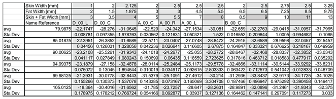
In order to characterize the dependence between the sample thickness, the irradiation frequency and the absorption, the measurements were averaged for several working frequencies. For each frequency, an average is performed in the spectral range of ±0.5 GHz. As part of the analysis, the average of the transmission coefficient S21 in this range and the standard deviation (measure of dispersion) of the results were calculated (see Table 3).
The results are summarized in the following graphs. For each frequency, the appropriate linear approximation was examined. For each graph, the values furthest from the trend line were examined. Values in the 80th percentile and below were omitted from the trend line. The graphs in Figure 18, Figure 19, Figure 20, Figure 21, Figure 22 and Figure 23 depict the trends, with a series of circles with a dashed linear approximation depicting an analysis of the entire population, and a series of diamonds with a continuous linear approximation depicting an analysis of the partial population.
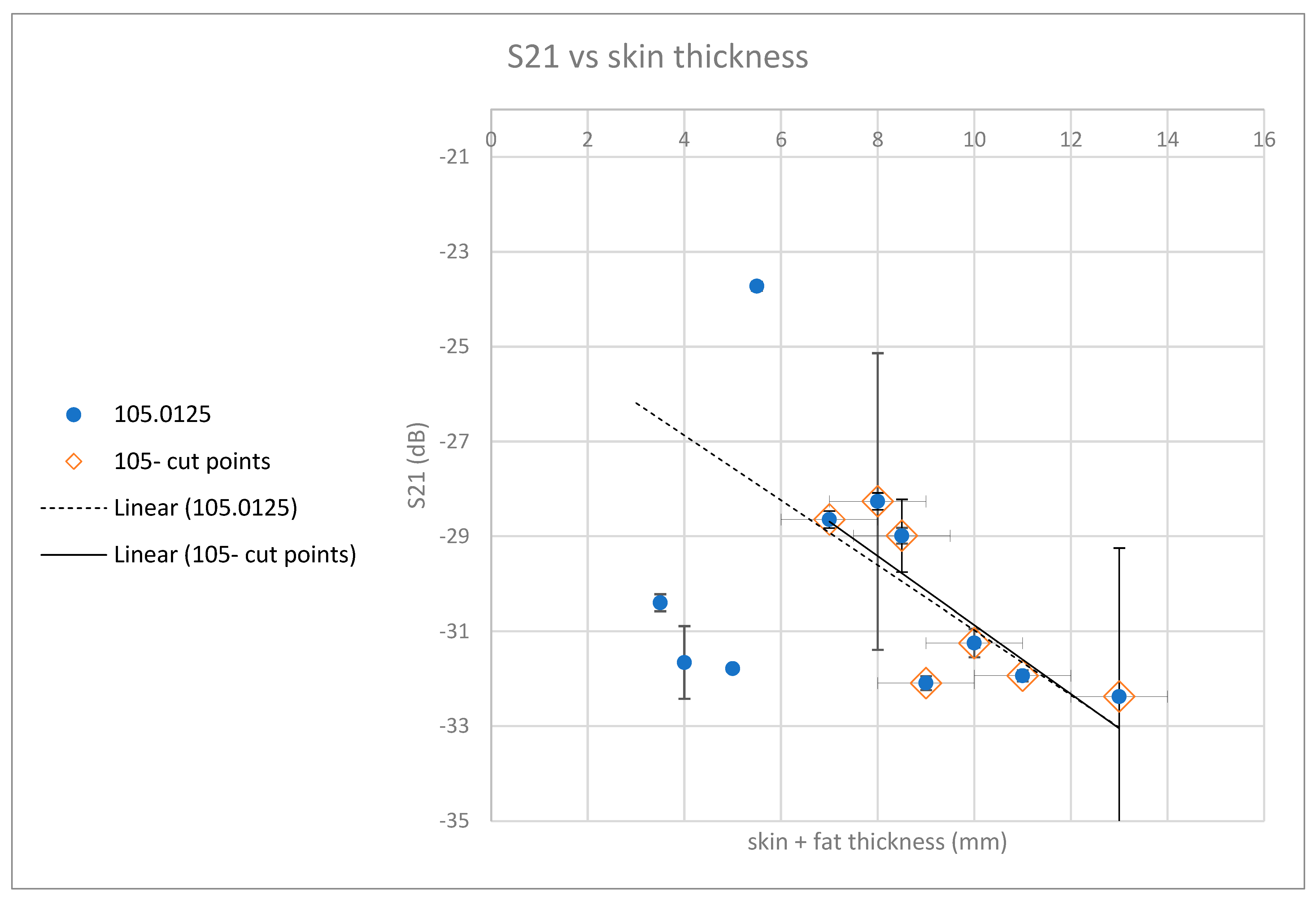
Figure 24.
S21 measurement around 105 GHz frequency vs. sample thickness.
Attenuation as function of sample thickness
Calculation of absorption - Based on the results of reflection and attenuation, the absorption of radiation in the various samples can be calculated according to the relationship:
S21 value measurements were averaged across the three measurement points in each sample separately for 0-degrees orientation. For 90-degrees orientation, the center point was considered.
Figure 25.
Calculation of absorption in all samples tested. A – 0-degree orientation, B – 90-degree orientation.
Figure 25.
Calculation of absorption in all samples tested. A – 0-degree orientation, B – 90-degree orientation.
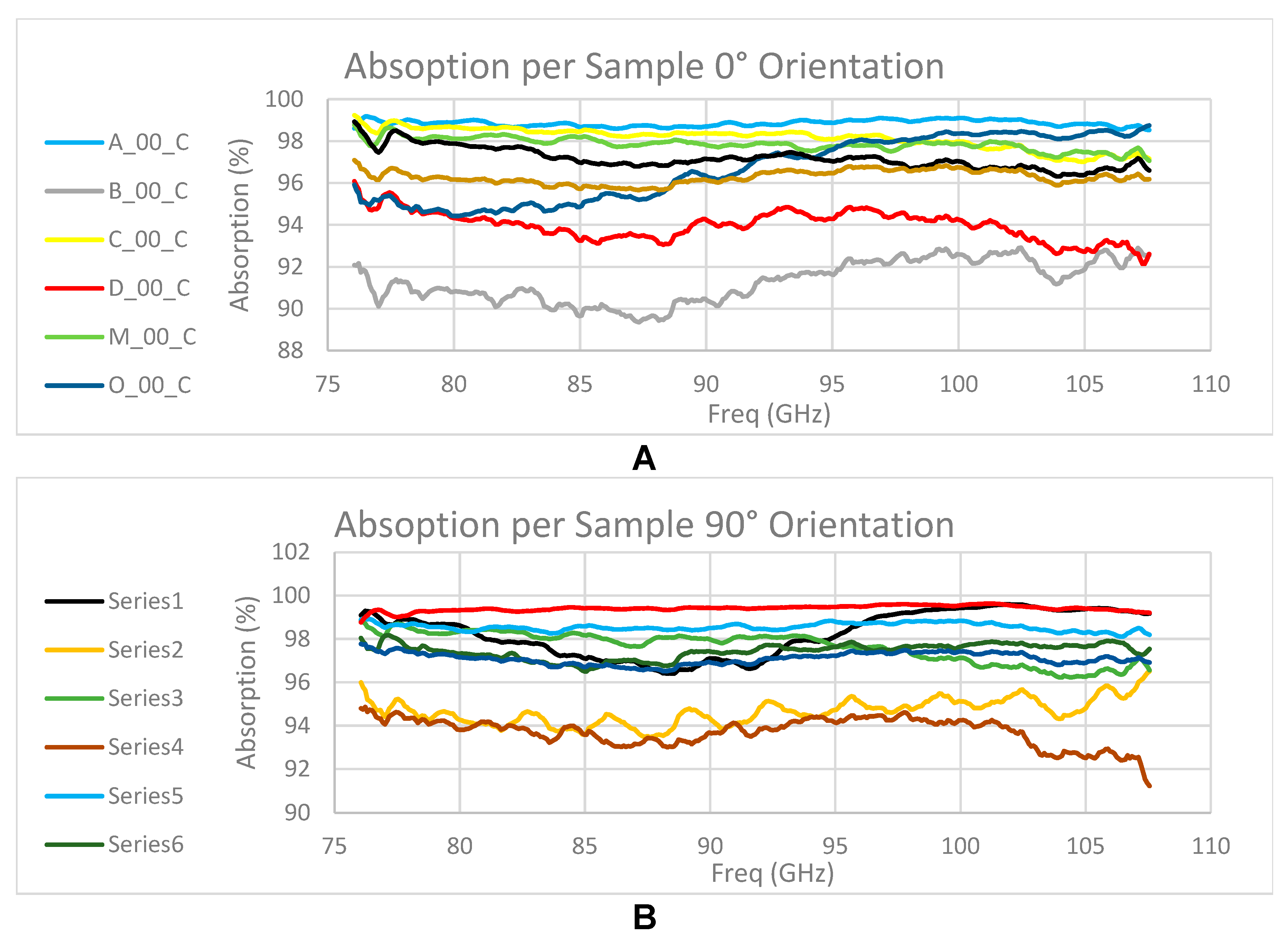
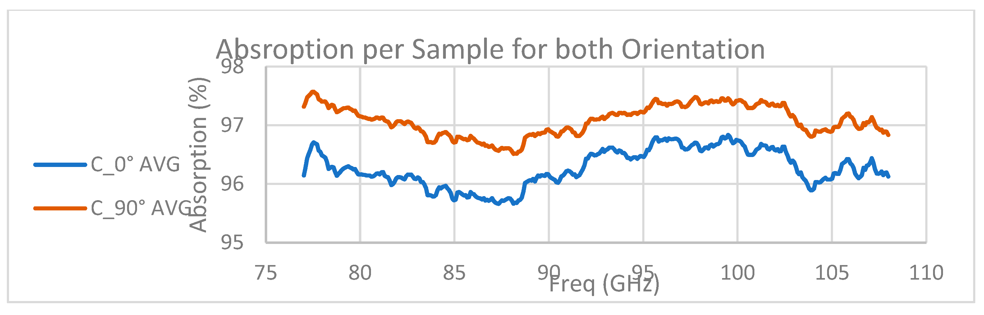
Figure 26.
Comparison between the two orientations. The lines are an average of the absorption values between all samples according to the measurement frequency.
Figure 26.
Comparison between the two orientations. The lines are an average of the absorption values between all samples according to the measurement frequency.
4. Discussion
S21 parameter representing attenuation in the passage through the medium indicates a high attenuation of -30 dB on average without significant dependence on reference points on the sample. The spectral behavior of the attenuation indicates monotonicity with slightly higher attenuation at high frequencies at 0-degree orientation (parallel to the direction of hair growth).
For a 90-degree orientation (horizontal polarization), higher variation can be seen between models, but on average the attenuation at high frequencies is lower than that in the 80-90 GHz range.
S11 parameter representing surface reflections indicates similar behavior in both polarizations. The values are between -10 and -20 dB, without significant frequency dependence for most samples, except for sample A in 0 orientation, and sample O in 90 orientation.
From the absorption calculations, it can be concluded that for the samples tested, absorption is significant in the skin and fat layer. The values for all samples range from 91% to 98% depending on the sample thickness. It should be noted that no significant dependence on frequency was observed.
To analyze the effect of orientation/polarization on absorption, a comparison of average absorption (between samples) in orientation 0 versus orientation 90 was performed. It can be seen that a consistent gap of between 0.8% to 1.2% is maintained at all frequencies in favor of absorption in an orientation perpendicular to the hair direction (orientation 90).
In order to assess the dependence of radiation transfer as a function of the sample thickness, an S21 parametric analysis was performed at the reference points while mapping over the skin and fat thickness at the measurement point. The graphs in the figure show the distribution of average values of radiation transfer (parameter S21) around different frequencies in the examined spectrum. The linear approximations calculated for the different samples show similar behavior at different frequencies when the radiation losses increases (from – -20 dB to -35 dB) with the thickness of the sample at a rate of 15 dB per 1 cm, comparable to what is obtained in our previous mice skin studies [23], and what is known about a water dominant volume [18].
5. Conclusions
Recommendations for further action
It is important to note the significant absorption rate in the skin and fat layer. It is not possible to calculate (based on the measurements performed) the contribution of each layer separately, but attenuation of over three orders of magnitude can be expected in penetration through the layer with a thickness of about 12 mm (-30dB).
The reflectance from the skin is similar at all frequencies. The values range from -10 to -20 dB probably depends on the texture of the skin. Therefore, most skin transfer loss is caused by absorption.
We plan to continue this study in order to analyze how long it takes to irradiate the cells to produce the expected clinical effect using the residual radiation (after attenuation and reflection) from a high-power gyrotron [13,16,17,22,24,25] or the FEL device [14,15].
At the same time, the temperature increase in the skin including epidermis as a result of radiation absorption during irradiation should be examined. We speculate that using short pulses can mitigate the problem to a significant extent.
Based on the analysis, it will become clear what clinical results can be achieved in external irradiation cancer treatment. Alternatively, implications for developing a transmission line that penetrates the skin can be examined.
Author Contributions
Conceptualization, M.E., S.D. and A.Y.; methodology, M.E. and S.D.; formal analysis, Y.S. and A.S.; investigation, Y.S., A.S., H.T..; resources, M.E. and A.Y.; data curation, Y.S. and A.S.; writing—original draft preparation, Y.S. and A.S.; writing—review and editing, A.Y.; visualization, Y.S. and A.S.; supervision, M.E., S.D. and A.Y.; funding acquisition, M.E. and A.Y. All authors have read and agreed to the published version of the manuscript.
Funding
This research was partially funded by the Israeli Ministry of Health grant # 20230409 “Cancer treatment using millimeter waves”.
Institutional Review Board Statement
Not applicable.
Informed Consent Statement
Not applicable.
Data Availability Statement
All data is available within the current paper.
Acknowledgments
The authors thank Boris Litvak from the Faculty of Engineering for his assistance in preparing and operating a system for measuring network parameters.
Conflicts of Interest
The authors declare no conflicts of interest.
References
- Jemal A, Siegel R, Ward E, Hao Y, Xu J, et al. (2009) Cancer statistics, 2009. CA: a cancer journal for clinicians 59: 225-249.
- Jemal A, Siegel R, Xu J and Ward E (2010) Cancer statistics, 2010. CA: a cancer journal for clinicians 60: 277-300.
- Wao H, Mhaskar R, Kumar A, Miladinovic B and Djulbegovic B (2013) Survival of patients with non-small cell lung cancer without treatment: a systematic review and meta-analysis. Syst Rev 2: 10. [CrossRef]
- Miyoshi N., Idehara T., Khutoryan E., Fukunaga Y., Bintang Bibin A., Ito S., and Sabchevski S.P. (2016) Combined Hyperthermia and Photodynamic Therapy Using a Sub-THz Gyrotron as a Radiation Source. Journal of Infrared, Millimeter, and Terahertz Waves pp 1-10. [CrossRef]
- Adey W R (1981) Tissue Interactions with Nonionizing Electromagnetic Fields. Physiological Reviews, Vol. 61 no. 2, 435-514.
- Apollonio F, Liberti M, Paffi A, Merla C, Marracino P, et al. (2013) Feasibility for Microwaves Energy to Affect Biological Systems Via Nonthermal Mechanisms: A Systematic Approach. Microwave Theory and Techniques, IEEE Transactions on 61: 2031-2045. [CrossRef]
- Pakhomov AG, Akyel Y, Pakhomova ON, Stuck BE and Murphy MR (1998) Current state and implications of research on biological effects of millimeter waves: a review of the literature. Bioelectromagnetics 19: 393-413.
- Paffi A, Apollonio F, Lovisolo GA, Marino C, Pinto R, et al. (2010) Considerations for Developing an RF Exposure System: A Review for in vitro Biological Experiments. Microwave Theory and Techniques, IEEE Transactions on 58: 2702-2714. [CrossRef]
- Fröhlich H (1968) Long-range coherence and energy storage in biological systems. International Journal of Quantum Chemistry 2: 641-649. [CrossRef]
- Rojavin MA and Ziskin MC (1998) Medical application of millimetre waves. QJM 91: 57-66.
- K. Komoshvili, J. Levitan, S. Aronov, B. Kapilevich and A. Yahalom “Millimeter Waves Non-Thermal Effect on Human Lung Cancer Cells”. The 3rd International IEEE Conference on Microwaves, Communications, Antennas and Electronic Systems (COMCAS 2011). November 7-9 (2011), 1D2-2.
- Komoshvili, K. et al. Morphological Changes in H1299 Human Lung Cancer Cells Following W-Band Millimeter-Wave Irradiation. Appl. Sci. 10, 3187 (2020). [CrossRef]
- Mariusz Hruszowiec, Wojciech Czarczyński, Edward F. Pliński, and Tadeusz Więckowski, "Gyrotron Technology", Journal of Telecommunications and Information Technology. 1(2014), 68, (2014). [CrossRef]
- A. Gover, A. Faingersh, A. Eliran, M. Volshonok, H. Kleinman, S. Wolowelsky, Y. Yakover, B. Kapilevich, Y. Lasser, Z. Seidov, M. Kanter, A. Zinigrad, M. Einat, Y. Lurie, A. Abramovich, A. Yahalom, Y. Pinhasi, “Radiation measurements in the new tandem accelerator FEL”, Nuclear Instruments and Methods A, Vol. 528, pp. 23-27 (2004).
- Y. Socol, A. Gover, A. Eliran, and M. Volshonok, Y. Pinhasi, B. Kapilevich, A. Yahalom, Y. Lurie, M. Kanter, M. Einat, and B. Litvak, "Coherence limits and chirp control in long pulse free electron laser oscillator", Physical review special topics – accelerators and beams Vol. 8, pp. 080701-1-9 , (2005). [CrossRef]
- M. Einat, M. Pilossof, R. Ben-Moshe, H. Hirshbein, and D. Borodin, "95-GHz gyrotron with ferroelectric cathode", Physical Review Letters, Vol. 109, P. 185101 (2012). [CrossRef]
- Moritz Pilossof and Moshe Einat, "A 95 GHz mid-power gyrotron for medical applications measurements", Review of Scientific Instruments 86, P. 016113, (2015). [CrossRef]
- Jonathan H. Jiang and Dong L. Wu "Ice and Water Permittivities for Millimeter and Sub-millimeter Remote Sensing Applications", Atmospheric Science Letters, October 6, 2004.
- Furman, O. et al. The Lack of Toxic Effect of High-Power Short-Pulse 101 GHz Millimeter Waves on Healthy Mice. Bioelectromagnetics 41, 188–199 (2020). [CrossRef]
- Komoshvili, K. et al. W-Band Millimeter Waves Targeted Mortality of H1299 Human Lung Cancer Cells without Affecting Non-Tumorigenic MCF-10A Human Epithelial Cells In Vitro. Appl. Sci. 10, 4813, 2020. [CrossRef]
- Barbora, A. et al. Non-Ionizing Millimeter Waves Non-Thermal Radiation of Saccharomyces cerevisiae—Insights and Interactions. Appl. Sci. 11, 6635 (2021). [CrossRef]
- Pilossof M., Einat M. (2018) 95-GHz Gyrotron With Room Temperature Dc Solenoid. In: IEEE Transactions on Electron Devices, vol. 65, no. 8, pp. 3474-3478. [CrossRef]
- Aronov S., Einat M., Furman O., Pilossof M., Komoshvili K., BenMoshe R., Yahalom A., Levitan J. (2018) Millimeter-wave insertion loss of mice skin. In: Journal of Electromagnetic Waves and Applications, vol. 32:6, pp. 758-767. [CrossRef]
- Kaczmarczyk L., Marsay K., Shevchenko S., Pilossof M., Levi N., Einat M., Oren M., Gerlitz G. (2021) Corona and polio viruses are sensitive to short pulses of W-band gyrotron radiation. In: Environ Chem Lett. vol. 19(6). pp. 3967-3972. [CrossRef]
- A. Shteinman, Y. Anker and Einat, (2024) Hard Rocks Absorption Measurements in the W-Band, J. Infrared Milli Tera Hertz Waves. [CrossRef]
Figure 1.
The experimental setup.
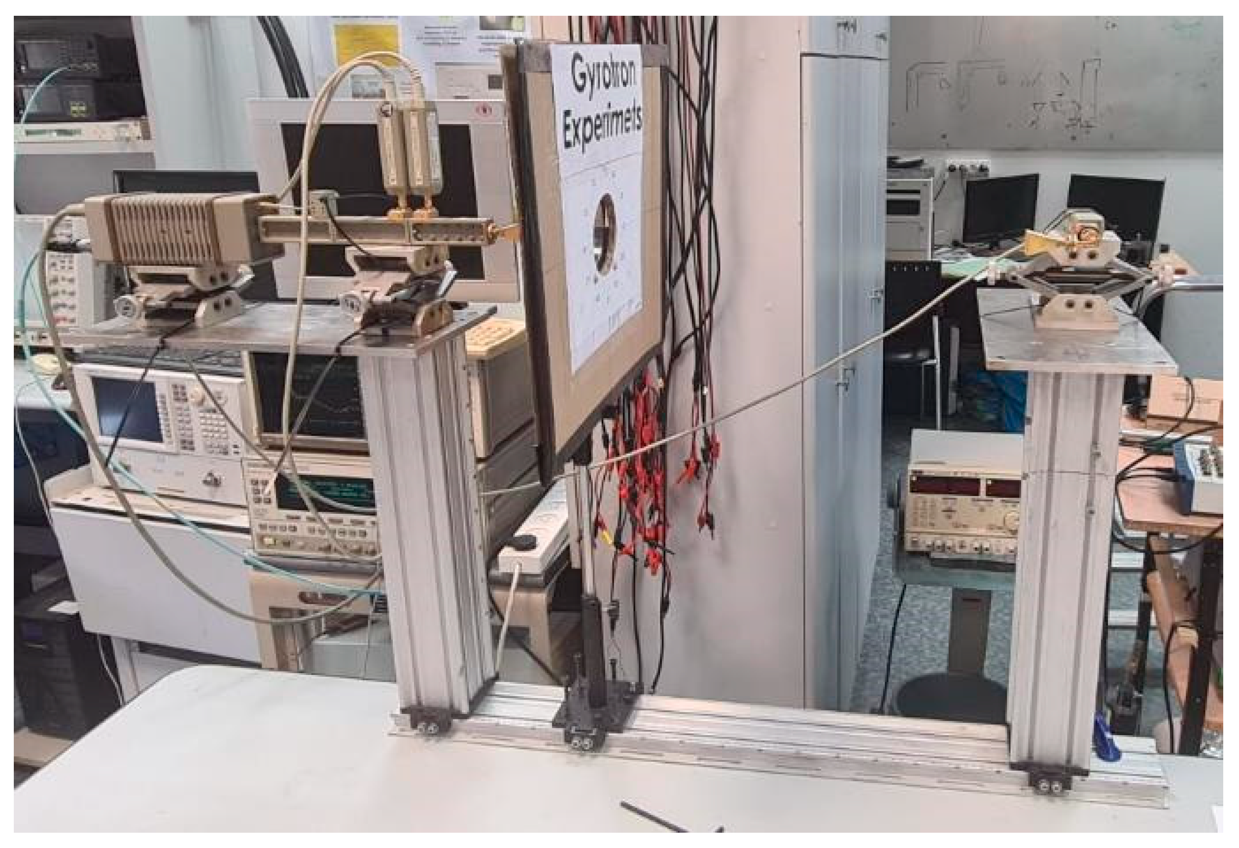
Figure 2.
Connection diagram of the experimental setup.
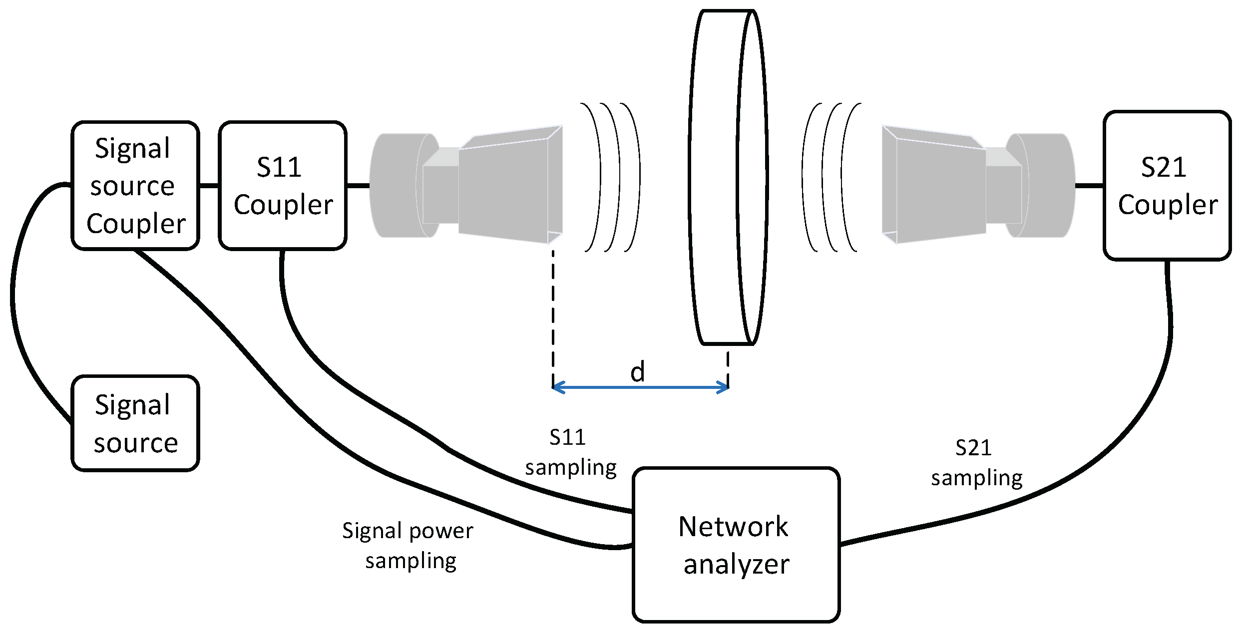
Figure 3.
Skin alignment.
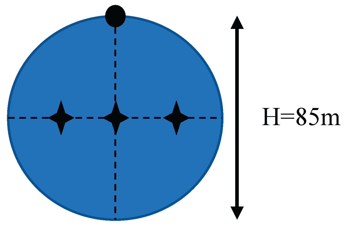
Figure 4.
Antenna structure diagram and the distances which must be considered.
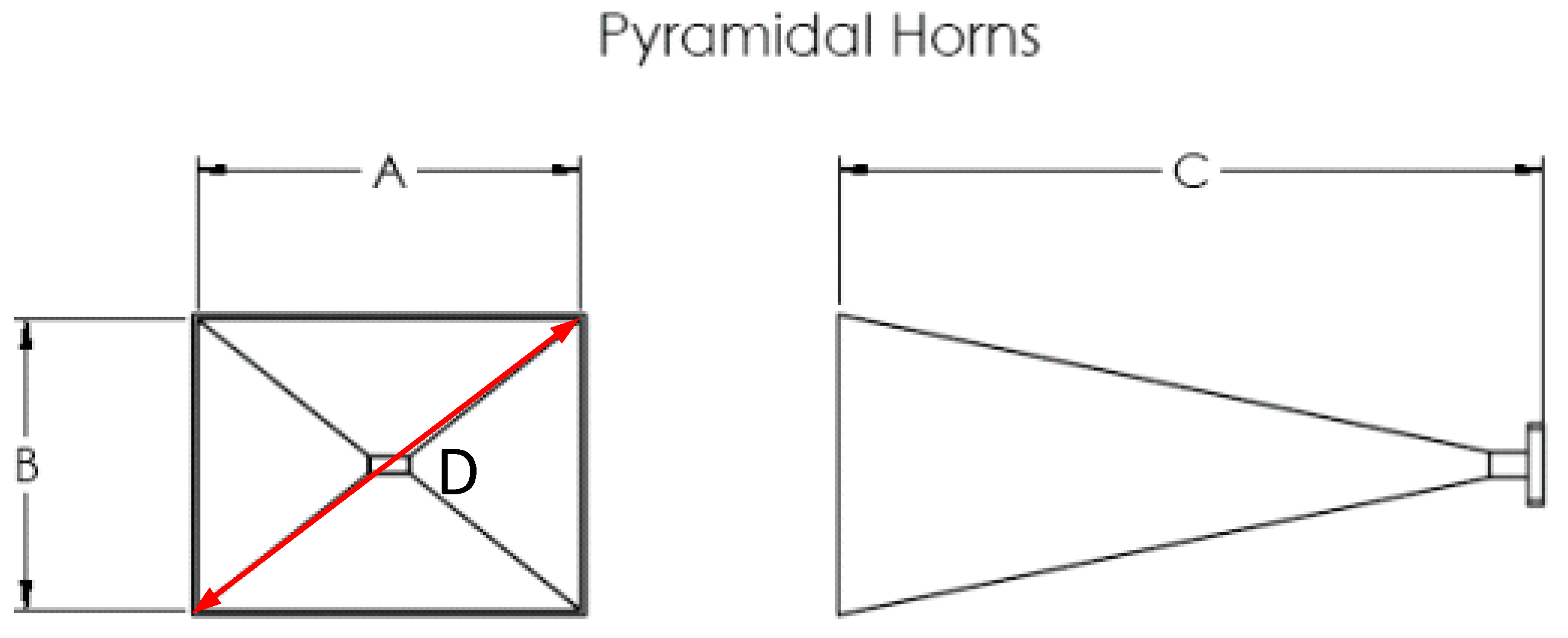
Figure 5.
Antenna dimensions breakdown - the highlighted line highlights the antenna used in the experiment.
Figure 5.
Antenna dimensions breakdown - the highlighted line highlights the antenna used in the experiment.
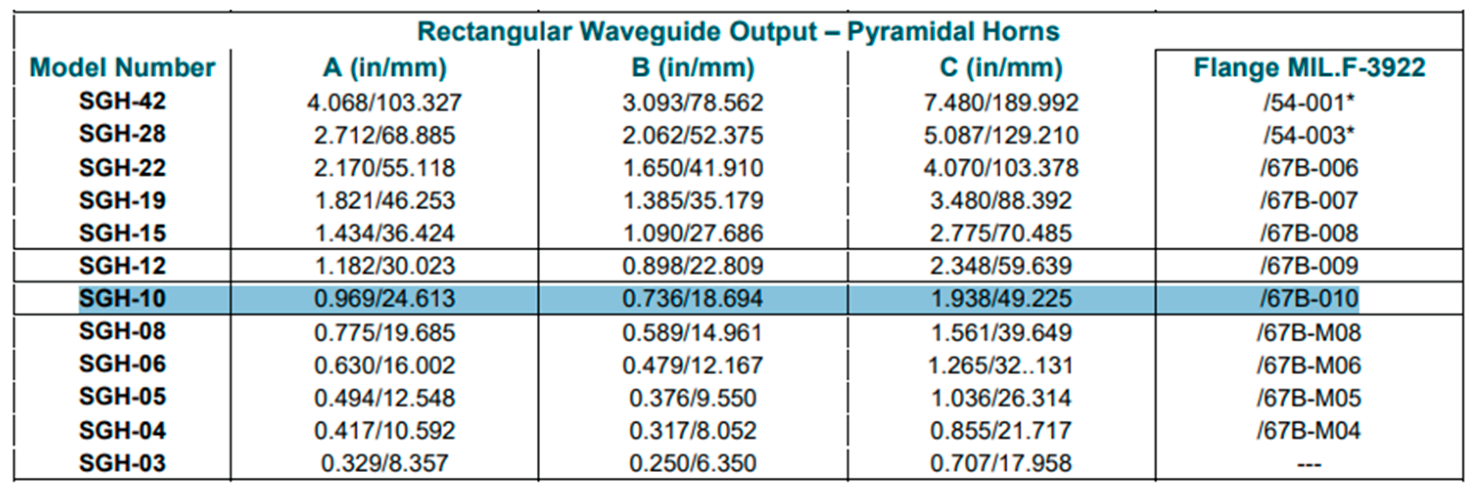
Figure 7.
The skin samples after cutting before embedding them in Petri dishes.
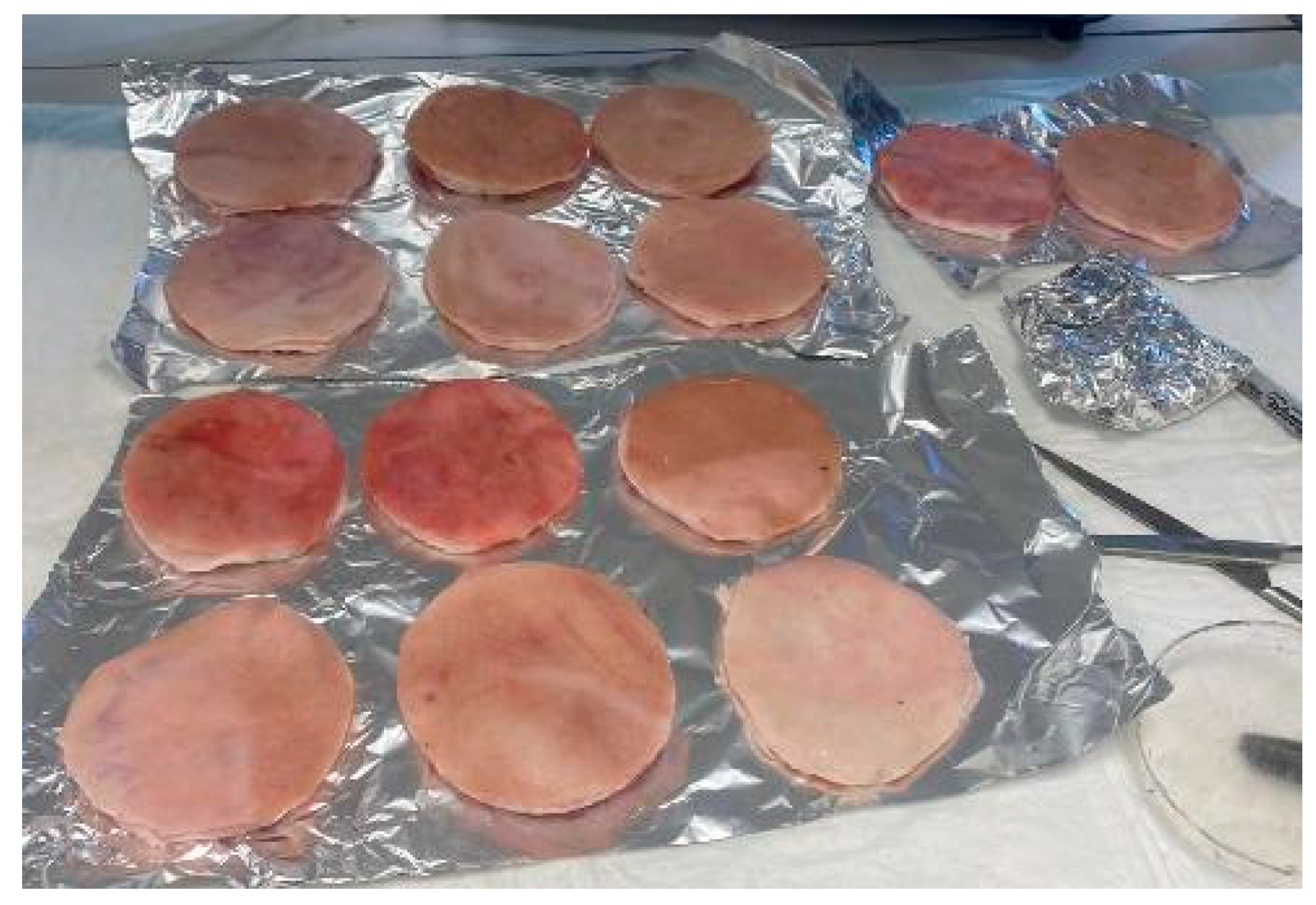
Figure 8.
Reference points on a Petri dish in two different samples.
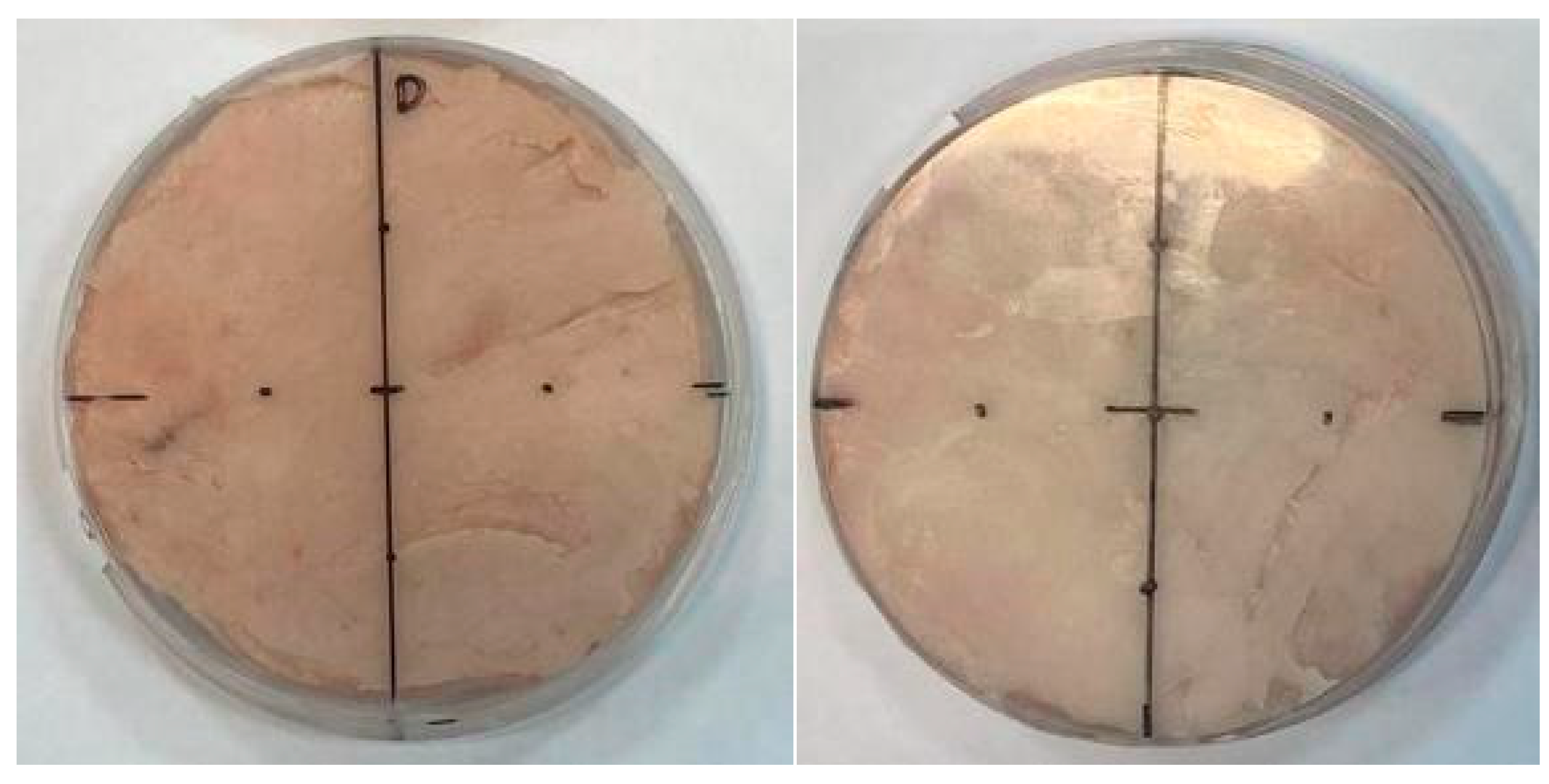
Figure 9.
Measurements of skin thickness and fat thickness. A - Measuring the thickness of the sample in a Petri dish, B - Estimating the skin thickness of the sample, C - Auxiliary device for measuring the height of the skin surface using a caliper.
Figure 9.
Measurements of skin thickness and fat thickness. A - Measuring the thickness of the sample in a Petri dish, B - Estimating the skin thickness of the sample, C - Auxiliary device for measuring the height of the skin surface using a caliper.
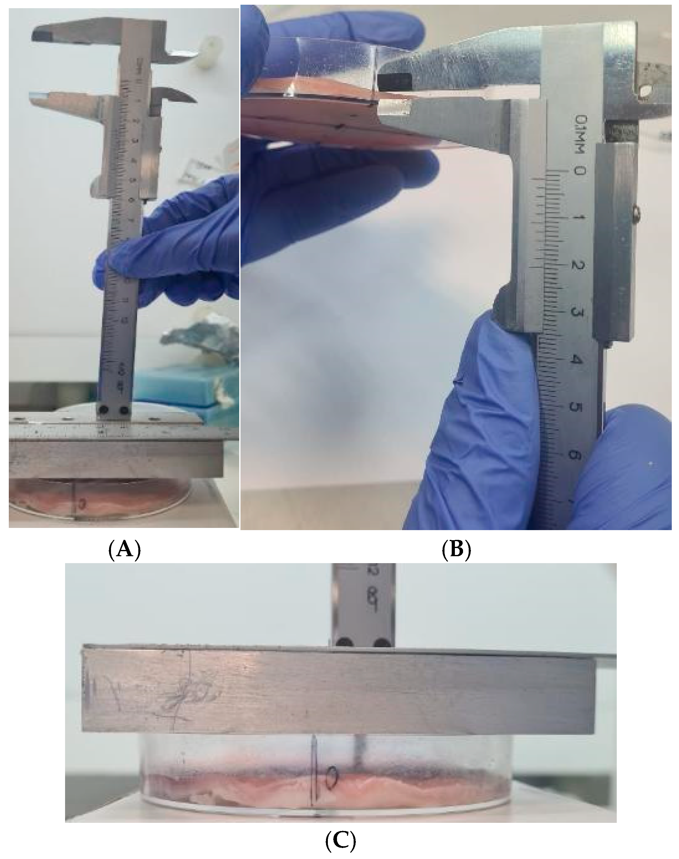
Figure 10.
Samples ready for measurement.
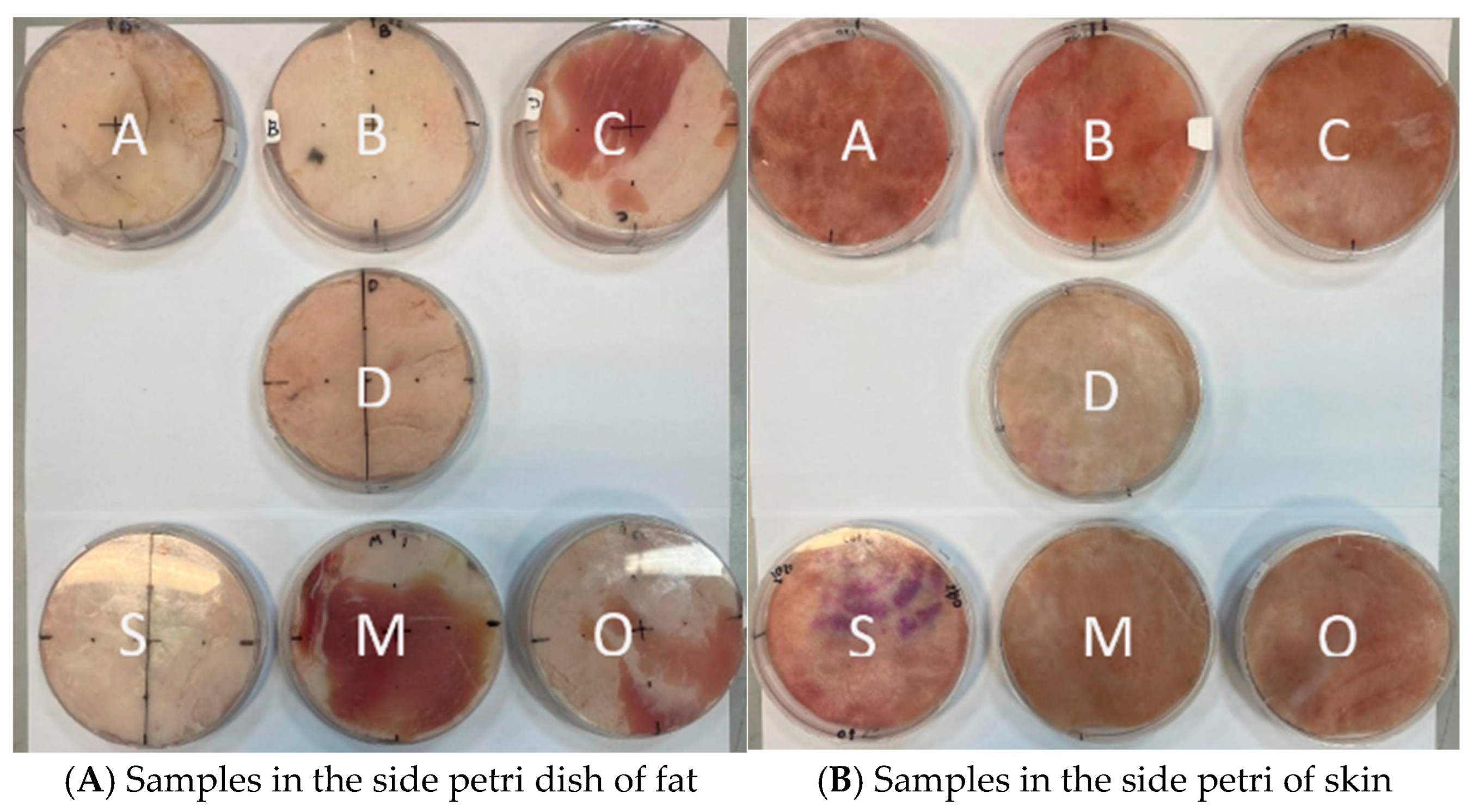
Figure 11.
Structure of the measurement setup built for the experiment.
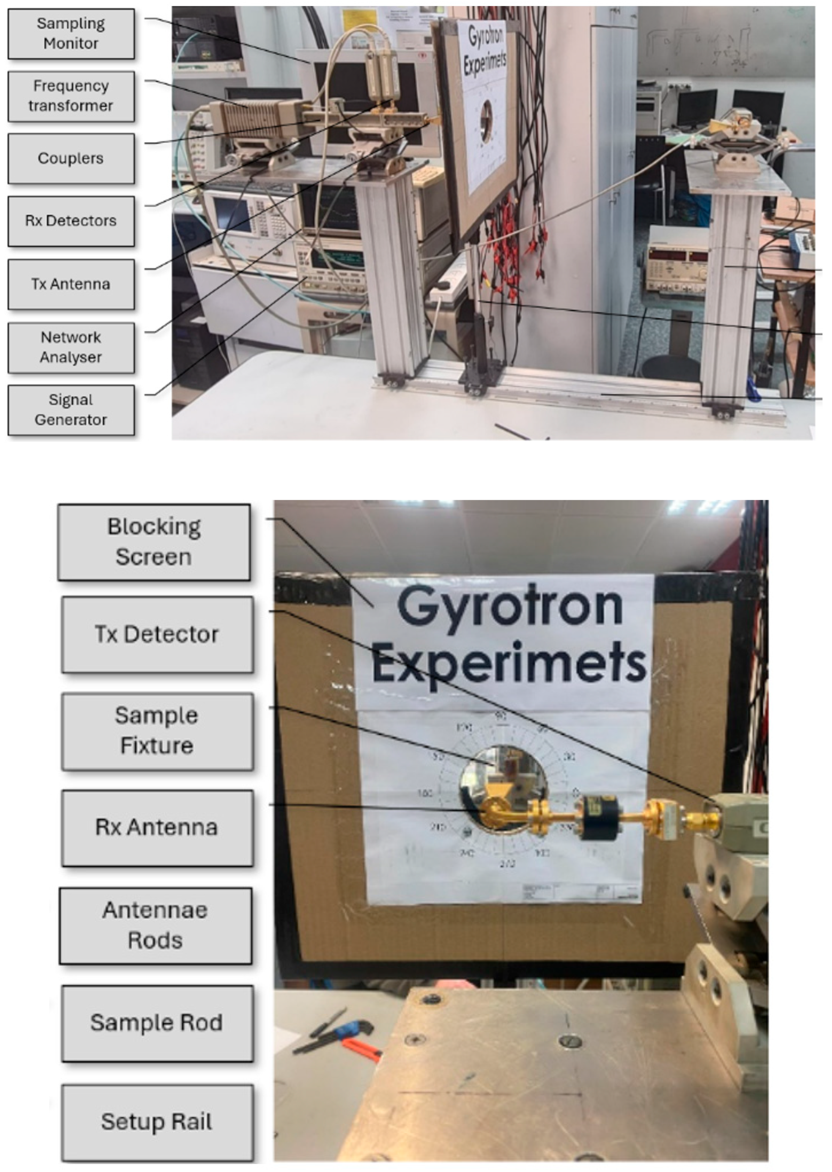
Figure 12.
Resetting the measurement array. Image A shows the adjustment in the position of the receiving and transmitting antennas. When the antenna posts and platforms were attached to the rail. Image B shows the complete array including an empty Petri dish. Inside the fixture on the sample column, the isolation screen (which blocks transmission around the sample) is installed around the sample and was used to calibrate the measurements.
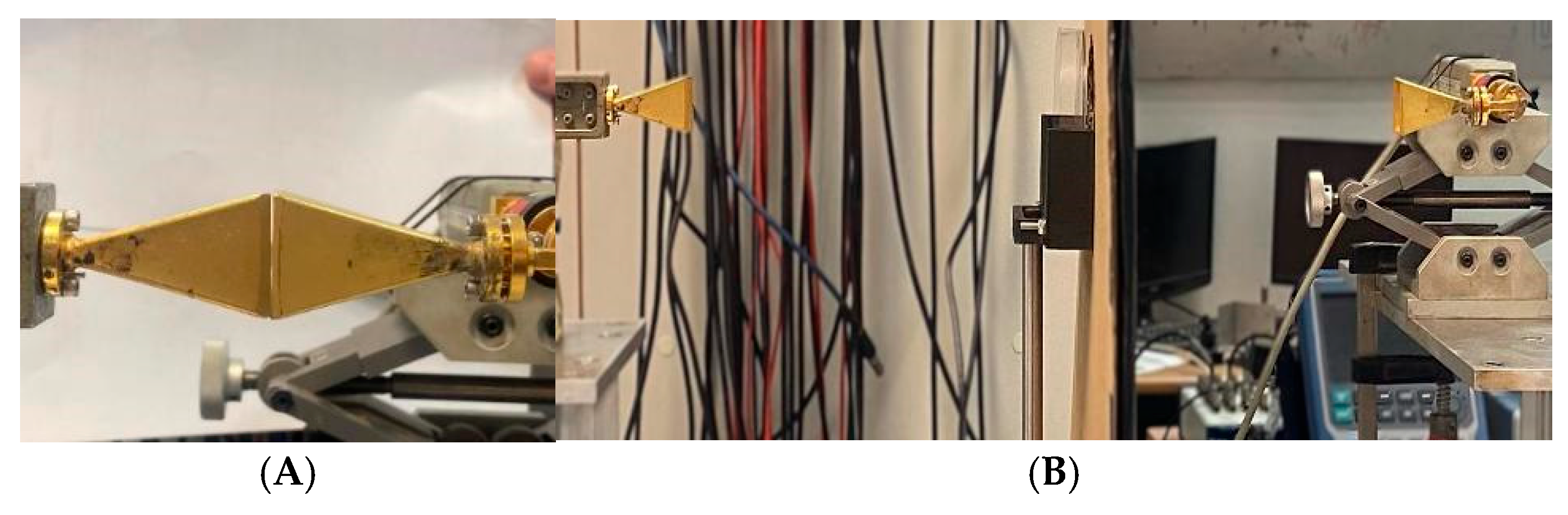
Figure 13.
Array calibration measurement for S21.
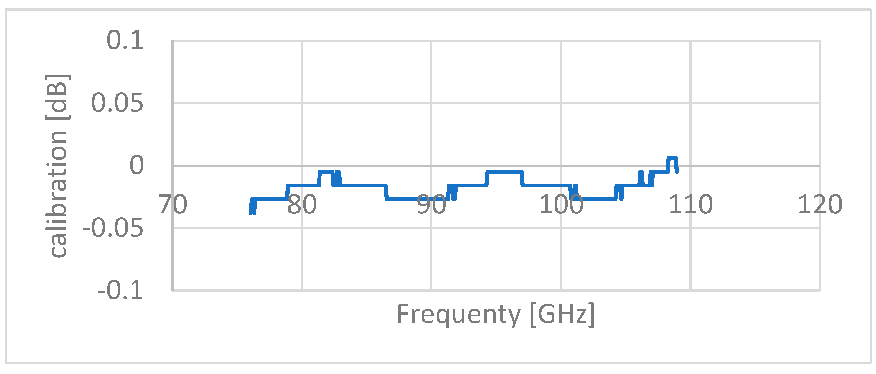
Figure 14.
Example of lateral displacement of the sample relative to the antenna axis. The right image (a) shows the array when the antenna axis passes through the center of the sample, and the left images (b, c) show the situation in which the sample has been moved to the right relative to the antenna axis (the central image from the transmitting antenna side and the left image from the receiving antenna side).
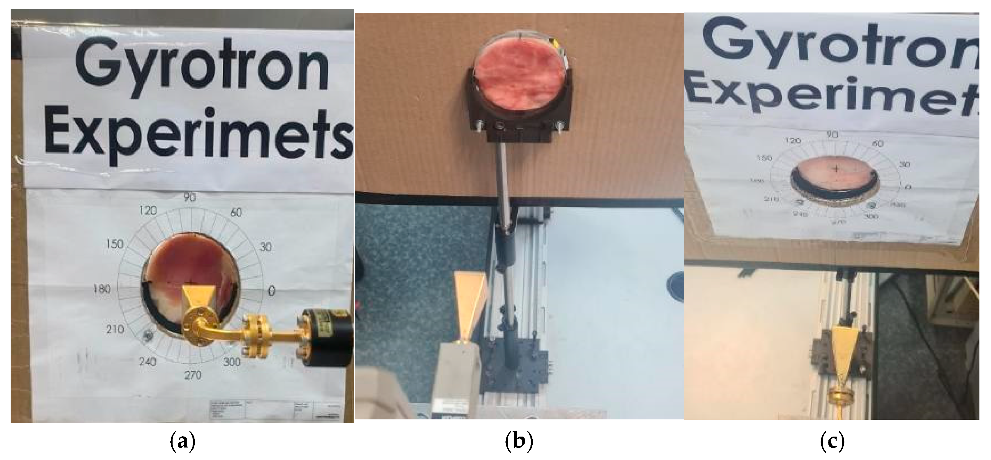
Figure 18.
Raw measurement S11: Measurements at the center of the sample. A – 0-degree orientation, B – 90-degree orientation. The light blue line shows the average over the measurements along the frequency axis.
Figure 18.
Raw measurement S11: Measurements at the center of the sample. A – 0-degree orientation, B – 90-degree orientation. The light blue line shows the average over the measurements along the frequency axis.
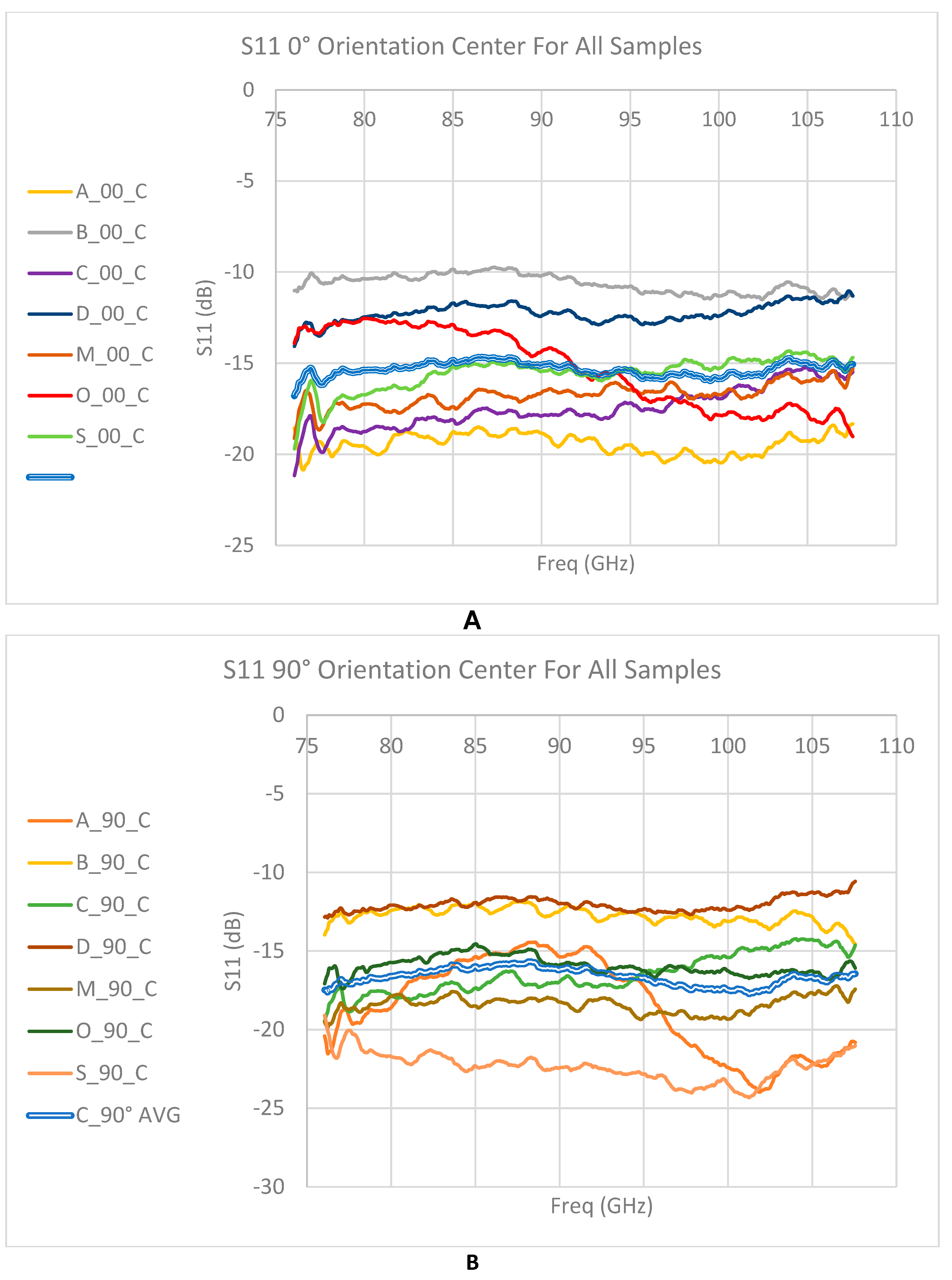
Figure 19.
S21 measurement around 80 GHz frequency vs. sample thickness.
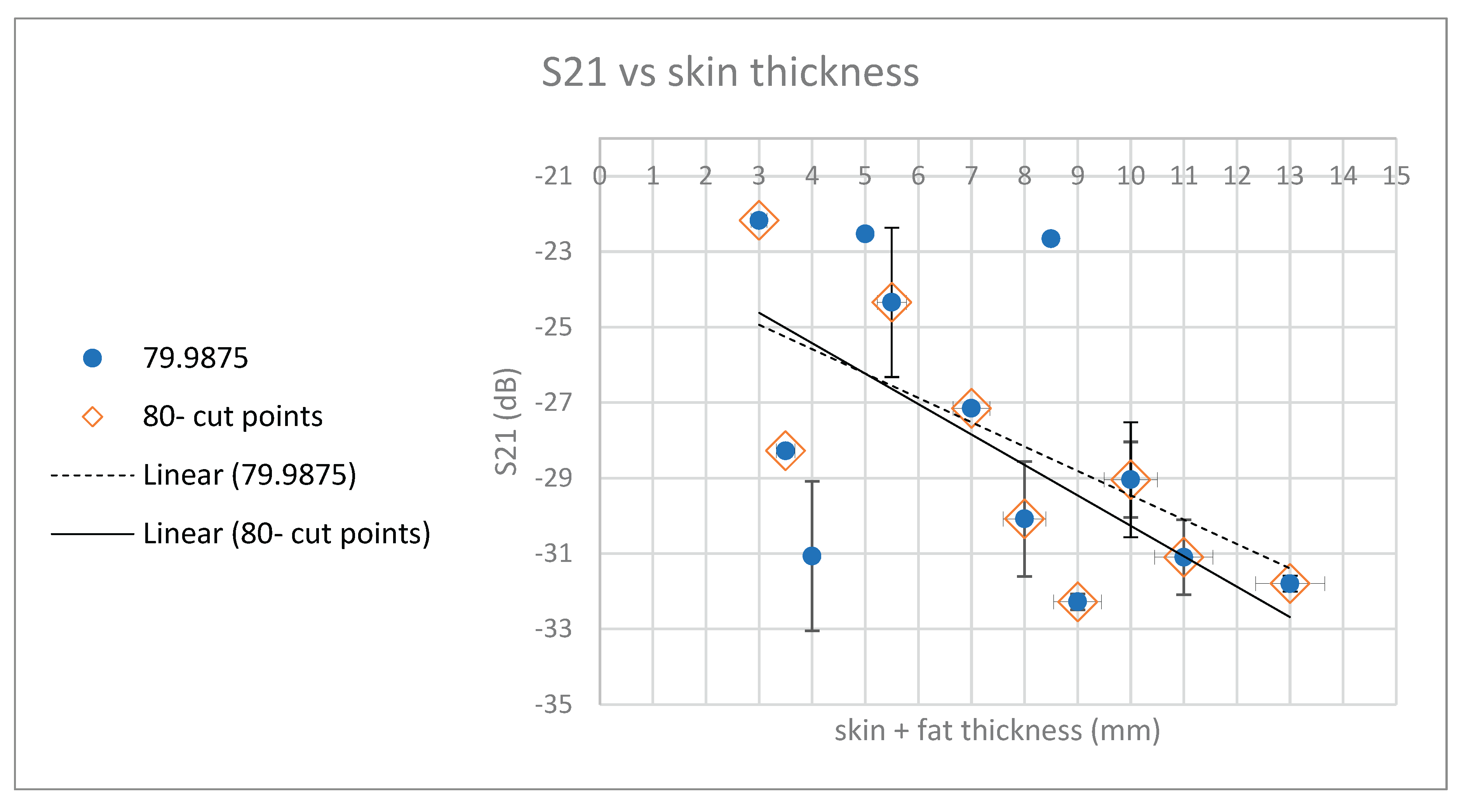
Figure 20.
S21 measurement around 85 GHz frequency vs. sample thickness.
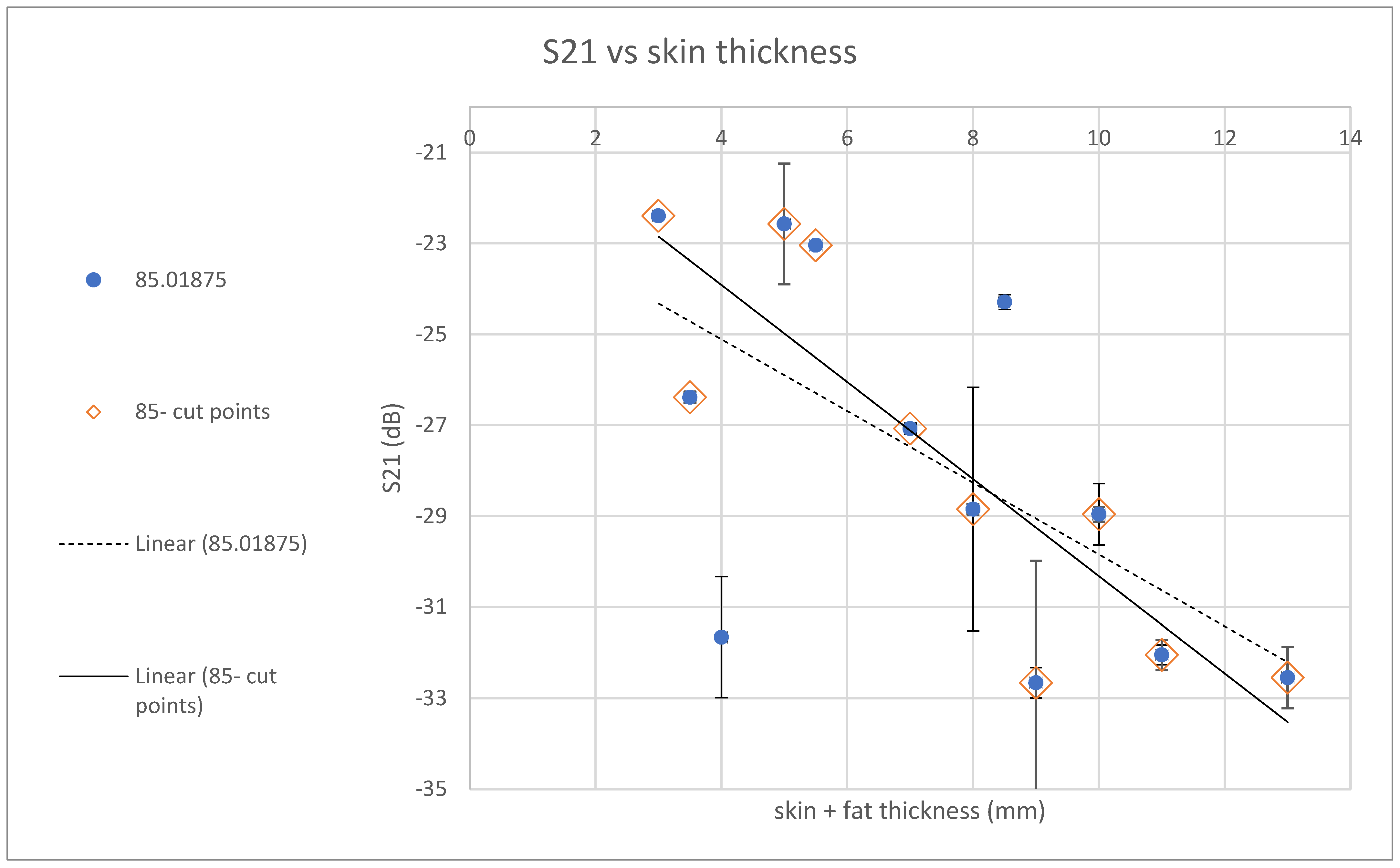
Figure 21.
S21 measurement around 90 GHz frequency vs. sample thickness.
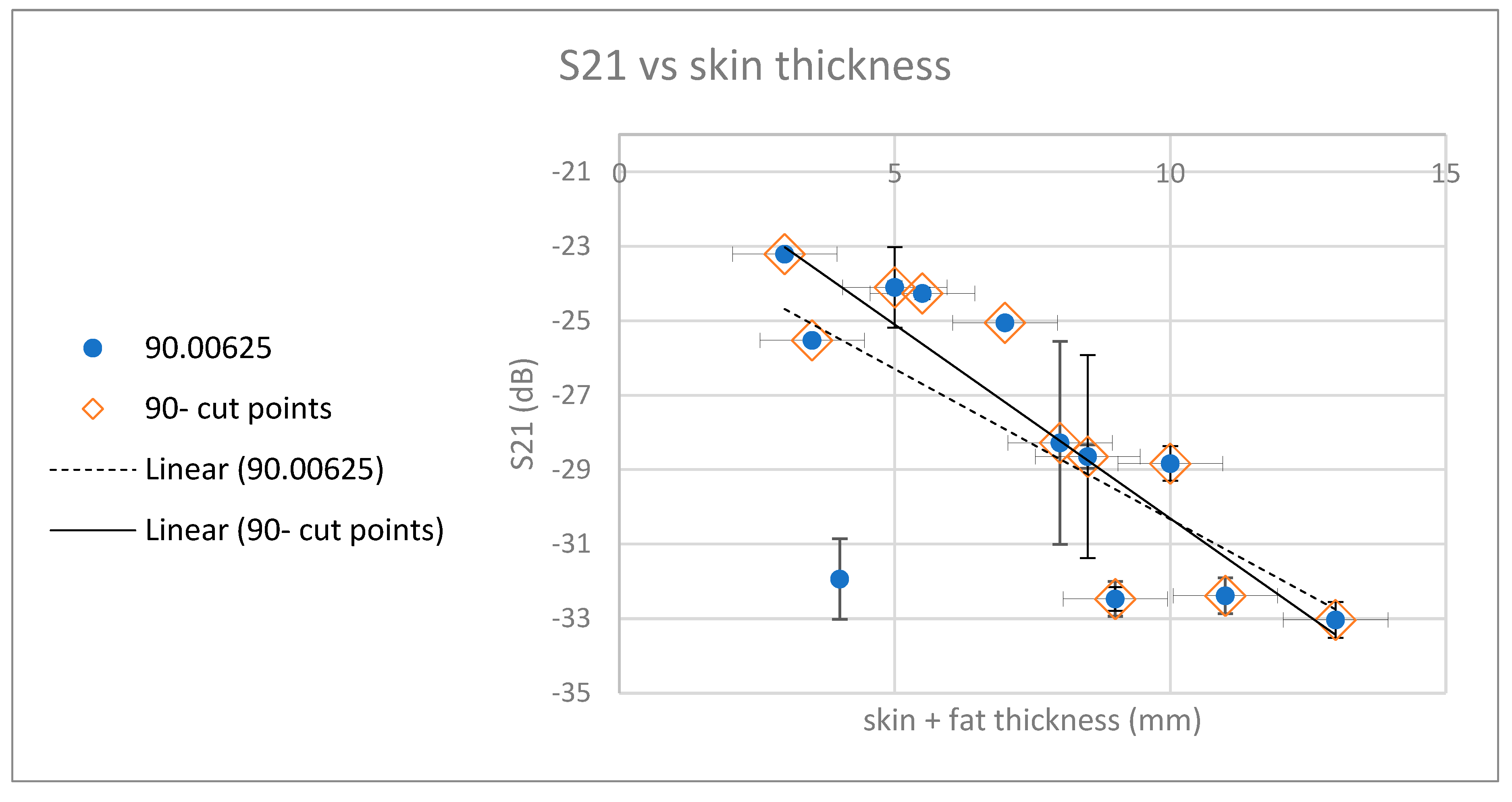
Figure 22.
S21 measurement around 95 GHz frequency vs. sample thickness.
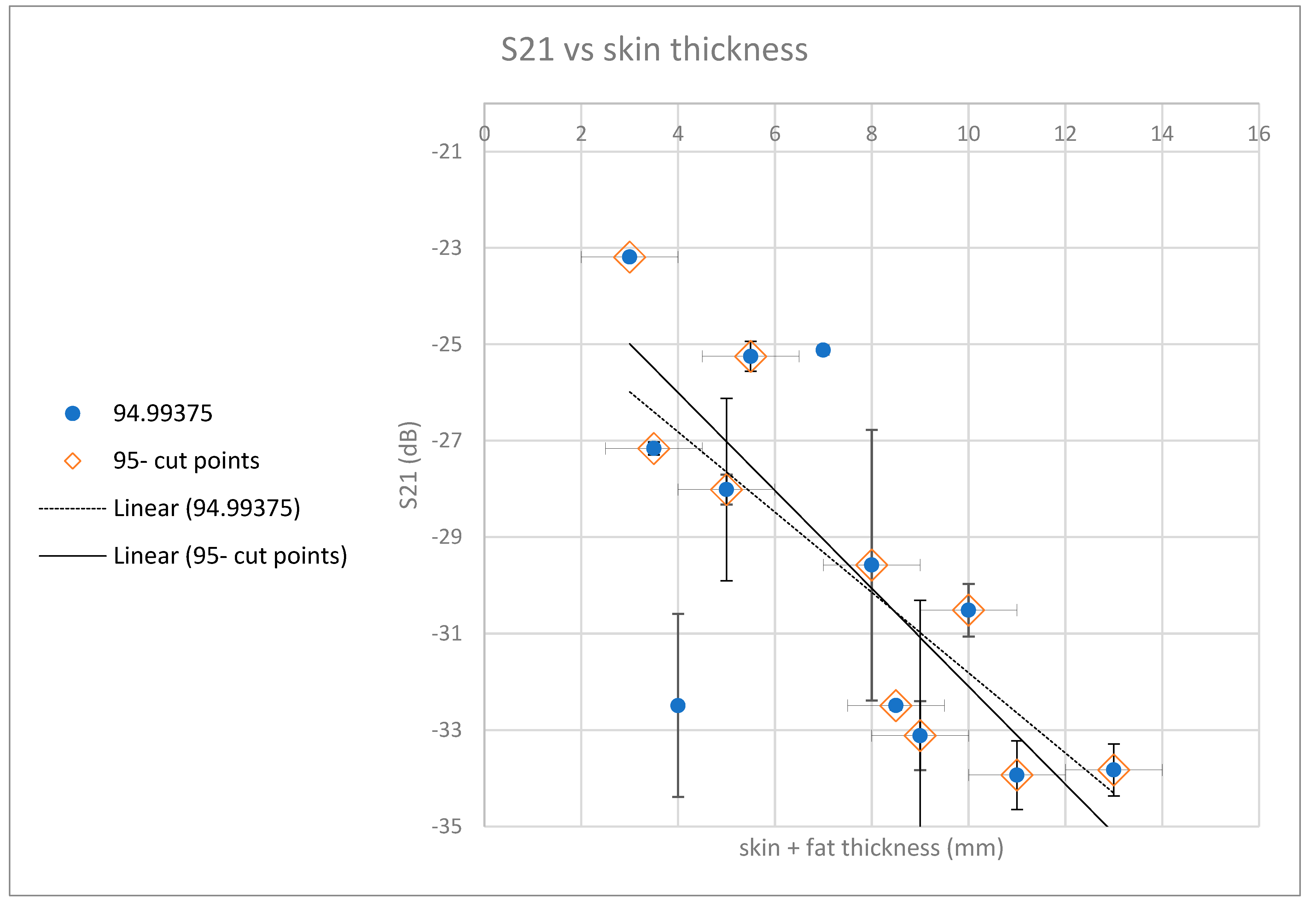
Figure 23.
S21 measurement around 100 GHz frequency vs. sample thickness.
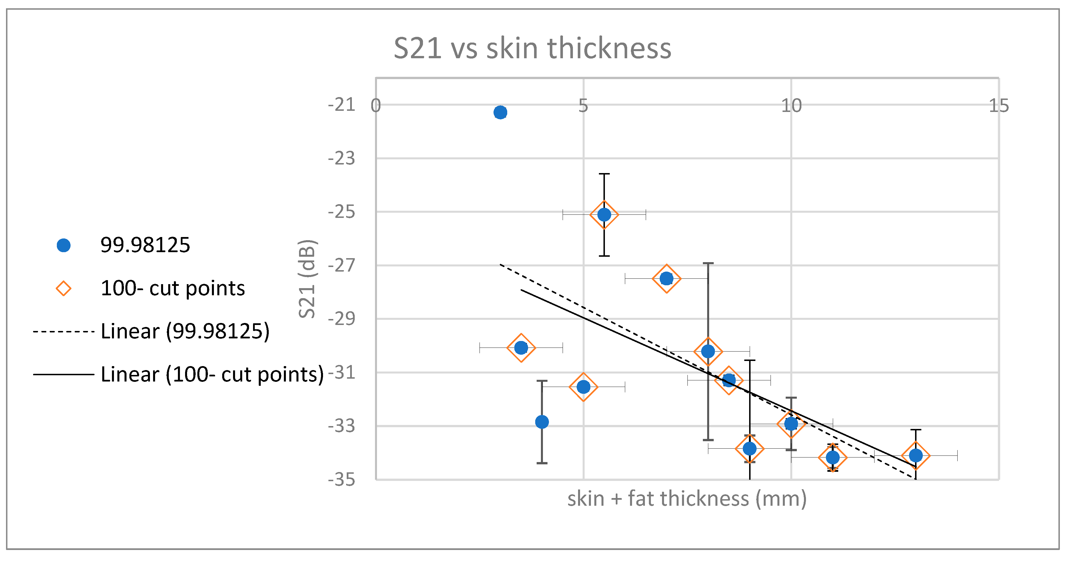
Table 1.
Summary of distances for measurements for each frequency.
| Frequency (GHz) | Wavelength (mm) | Far field limit (mm) | Reactive near field limit (mm) |
| 75 | 4 | 477.6 | 53.27 |
| 95 | 3.158 | 605 | 59.95 |
| 110 | 2.727 | 700 | 64.51 |
Table 3.
Analysis of the dispersion of S21 values for representative frequency bands segmented by samples thickness at the measurement point.
Table 3.
Analysis of the dispersion of S21 values for representative frequency bands segmented by samples thickness at the measurement point.
Disclaimer/Publisher’s Note: The statements, opinions and data contained in all publications are solely those of the individual author(s) and contributor(s) and not of MDPI and/or the editor(s). MDPI and/or the editor(s) disclaim responsibility for any injury to people or property resulting from any ideas, methods, instructions or products referred to in the content. |
© 2025 by the authors. Licensee MDPI, Basel, Switzerland. This article is an open access article distributed under the terms and conditions of the Creative Commons Attribution (CC BY) license (http://creativecommons.org/licenses/by/4.0/).
Copyright: This open access article is published under a Creative Commons CC BY 4.0 license, which permit the free download, distribution, and reuse, provided that the author and preprint are cited in any reuse.


