
Submitted:
06 November 2025
Posted:
07 November 2025
You are already at the latest version
Abstract
Exploring Pareto-optimal trade-offs in analog circuit design is computationally expensive because each candidate evaluation requires time-consuming SPICE simulations. We propose a surrogate-augmented multi-objective optimization framework supporting two operational modes: Surrogate-Guided Optimization (SGO) with periodic truth validation, and Multi-Fidelity Optimization (MFO) with adaptive fidelity promotion. Our pipeline embeds a Graph Neural Network (GNN) surrogate within standard multi-objective evolutionary algorithms (NSGA-II, NSGA-III, SPEA2, MOEA/D) and couples: (i) simu-lator-in-the-loop data generation with caching, deduplication, and selective parallel dispatch of SPICE evaluations via process-based or distributed execution; (ii) uncertain-ty-aware fidelity control with checkpoint/rollback governance to bound predictive drift, tracking Mean Absolute Error (MAE) across validation batches; and (iii) diversity-aware truth selection strategies (greedy farthest-point or crowding distance) that target in-formative regions of the design space. Both operational modes are evaluated across four representative operational amplifier topologies under uniform configurations. The pro-posed approach lowers the number of high fidelity simulations required while main-taining comparable Pareto front quality, indicating a pragmatic path to more sam-ple efficient analog optimization without relying on large scale pretraining or transfer learning.
Keywords:
surrogate modelling
; multiobjective optimization
; simulator-in-the-loop
; neural networks
; hyperparameter optimization
; analog circuit design
1. Introduction
The optimization of analog and RF circuits is a computationally demanding task due to the high fidelity and physics accuracy required from circuit simulators such as SPICE. The design process typically involves satisfying multiple, often conflicting objectives—such as gain, bandwidth, noise, power consumption, and silicon area—while simultaneously meeting strict performance constraints. Multiobjective evolutionary algorithms (MOEAs), such as the Non-dominated Sorting Genetic Algorithm II (NSGA-II) and its many successors [1,2], have been widely adopted to explore such complex trade-offs. Their population-based search enables broad coverage of the design space and the generation of Pareto-optimal fronts that quantify performance trade-offs. However, when each candidate evaluation requires a full SPICE simulation, the computational cost becomes prohibitive.
To mitigate this bottleneck, surrogate-assisted optimization (SAO) strategies have emerged [3,4,5,6,7]. In these methods, a predictive model—known as a surrogate—approximates the mapping from design parameters to circuit performance, reducing the need for expensive simulator calls. Early surrogates were often based on Gaussian processes (GPs) or radial basis function (RBF) models, valued for their accuracy in low-dimensional settings and ability to provide uncertainty estimates [3,6]. However, these approaches do not scale well to high-dimensional parameter spaces or to large, heterogeneous training datasets. More recent work has explored neural-network-based surrogates, including multilayer perceptrons (MLPs) [8,9,10] and topology-aware architectures such as graph neural networks (GNNs) [11,12,13], which can directly encode the structural information of circuit schematics.
Several research directions have evolved within this space. One major line of work focuses on Bayesian optimization (BO) for analog circuit synthesis, often combining neural feature extractors with probabilistic acquisition functions [8,14,15,16]. BO methods offer strong sample efficiency but tend to be less suited to finding a diverse Pareto front in high-dimensional, multiobjective settings without substantial adaptation [17]. Another line pursues large-scale surrogate modeling, where models are trained on broad set of simulated designs—sometimes spanning many circuit families—to obtain reusable predictors for selected analog front-end topologies [12,18]. For example, LASANA [12] targets fast SPICE replacement for particular analog sub-blocks. Conversely, INSIGHT [18] employs an autoregressive Transformer to deliver a technology-independent, higher-fidelity neural simulator across several analog front-end circuits and process nodes, giving it a “foundation-like” character within that narrow domain, but still short of the breadth and cross-domain adaptability associated with true foundation models.
Evolutionary computation remains central to analog circuit optimization [1,2,19], and hybrid approaches that couple MOEAs with surrogates—known as surrogate-assisted evolutionary algorithms (SAEAs)—have been extensively studied [3,4,5]. These include methods that integrate surrogate uncertainty into selection, dynamically switch between fidelity levels, or use multi-fidelity surrogates to exploit both fast low-accuracy models and expensive but high-accuracy models [6,20,21,22]. Yet, the majority of SAEAs in the circuit-design literature remain task-specific, requiring the surrogate to be retrained from scratch for each new circuit topology or specification set, and often relying on small, narrowly distributed datasets.
Building on these advances, the present work unifies large-scale surrogate modelling, uncertainty-aware evolutionary optimization, and active simulator validation into a coherent framework designed for analog circuit synthesis. More specifically, the proposed framework combines:
Multi-surrogate model layer: Rather than pre-training a large foundation model, we introduce a multi-surrogate reconfigurable model based on ensemble learning and GNN trained and incrementally updated on run-specific Ngspice [23] data (with optional warm-start) covering multiple circuit families and parameter distributions. This model is designed for rapid adaptation (fine-tuning) to new targets with minimal additional simulations.
Simulator-in-the-loop orchestration: The surrogate is embedded in a multi-fidelity optimization loop that periodically validates and corrects predictions with Ngspice simulations, ensuring that model drift and overconfidence are detected and mitigated. The loop also includes deterministic caching, deduplication, and selective parallel dispatch of uncached simulations, and drives early stopping via dual convergence metrics—hypervolume (HV) expansion and raw IGD reduction—to monitor Pareto spread and proximity while detecting drift or overconfidence.
Uncertainty-aware control: Predictions are augmented with explicit epistemic uncertainty estimates, which are incorporated into both penalization and fidelity selection, improving robustness against erroneous surrogate optima.
Active acquisition and co-tuning: Optional active learning queries and DoE (Design of Experiments) seeding (correlated LHS, mixed strategies) are coupled with Optuna1 [24] joint tuning of surrogate and NSGA-II hyperparameters, adaptively steering both data collection and Multiobjective search dynamics online.
Extensibility and reproducibility: The platform is designed as a modular, component-oriented system with strong governance features—event manifests, structured logging, and schema-controlled data storage—supporting reproducibility, auditability, and rapid experimentation.
To summarize, this work introduces a unified framework that reduces dependence on costly SPICE evaluations while preserving Pareto-front quality. In the following section, we describe the software architecture supporting this framework, highlighting how its layered design integrates simulation, surrogate modeling, and multiobjective optimization into a coherent and extensible platform.
2. Materials and Methods
The simulator has been designed as an integrated software platform that combines a modular architecture with advanced optimization strategies to accelerate circuit design exploration. This section describes in detail the system’s internal organization and workflow, from its software architecture and module orchestration to its simulation lifecycle and optimization loop. Particular attention is given to the closed-loop surrogate-assisted optimization framework, which minimizes reliance on expensive SPICE evaluations while maintaining accuracy through uncertainty calibration and adaptive fidelity control. In addition, supporting mechanisms such as result caching and selective reuse of past evaluations are included to further reduce redundant computations and improve efficiency.
The optimization engine supports multi-objective evolutionary search strategies such as NSGA-II, MOEA/D, SPEA2, and NSGA-III, which are tightly coupled with active learning routines interleaving uncertainty-, diversity-, and performance-driven acquisition. Surrogate modeling integrates both an ensemble of regressors and an optional circuit-aware graph attention network, enabling the framework to capture structural dependencies in circuits while yielding calibrated uncertainty estimates. An adaptive fidelity controller escalates surrogate predictions to SPICE only when confidence falls below a dynamic threshold, applying soft penalties to discourage overconfident but unverified regions. The data layer is manifest-driven and built upon SQLite with structured artifacts, ensuring deterministic replay, version tagging, and full provenance of every evaluation. Concurrency-safe caching, deduplication, and eviction policies reduce redundant simulations even under parallel workloads. Early search stages are accelerated through design-of-experiments seeding with space-filling and constraint-aware sampling, fostering rapid Pareto front formation before adaptive refinement dominates. The optimization driver orchestrates iterative propose–evaluate–verify cycles, retrains surrogate ensembles, and recalibrates uncertainty estimates on-the-fly. Finally, a modular plugin interface allows new algorithms, acquisition functions, surrogates, or visualizers to be added without altering the execution pipeline, while command-line automation and reproducible configuration files support batch experimentation.
2.1. System Architecture
The proposed platform is built around a layered, component-oriented architecture that cleanly separates the concerns of multiobjective optimization, surrogate modeling, and circuit simulation. This separation of responsibilities is key to achieving both modularity—so that each component can be replaced or extended without affecting the others—and reproducibility, ensuring that every optimization run can be reconstructed from its logged configuration and outputs (Figure 1).
At the top level, the optimization layer implements a modular multiobjective evolutionary algorithm engine, with NSGA-II [1] and MOEA/D as its primary backends. This layer abstracts the core tasks of decision-variable encoding, objective-vector construction, constraint handling, and population archiving. It integrates convergence-control mechanisms, such as hypervolume-based early stopping and deterministic seeding, without interfering with lower-level modules. This design allows to rapidly swap or tune optimization algorithms without having to modify the simulation or surrogate layers.
The optimization layer delegates each generation to a multi-fidelity controller that mediates between fast surrogate predictions and high-fidelity (HF) Ngspice simulations. All candidate designs are first scored and assigned predicted objectives plus uncertainty; configurable selection policies (uncertainty ranking, hybrid scoring, or hypervolume-proxy blending) then choose a subset for high-fidelity verification. Those selected simulations currently run sequentially while the unselected designs retain their surrogate-predicted values. A generation completes only after every chosen high-fidelity run finishes, preserving clear iteration boundaries. Parallel SPICE execution is, at present, limited to the single-fidelity mode when explicitly enabled; extending parallelism to the multi-fidelity verification subset is a planned enhancement. This separation of “which designs to verify” from “how they are simulated” allows future evolution of selection strategies without disruptive architectural changes.
Central to the platform is the surrogate subsystem, The platform’s surrogate subsystem can use either a lightweight ensemble (default) or an optional graph neural network (GNN) model able to encode circuit connectivity; both provide predicted objective values together with an uncertainty signal for each design. During optimization the surrogate is updated incrementally with newly validated high-fidelity results; when accuracy improves beyond a configured margin a checkpoint is saved, and if quality degrades beyond a tolerance an earlier state can be restored. An adaptive uncertainty penalty adjusts unvalidated objective estimates using a dynamically tuned weight that balances exploring uncertain regions against exploiting promising ones. Improvement, rollback, and penalty adjustment events are recorded so a run can be audited, and a manifest summarizing this history is emitted when run artifact output is enabled. An active acquisition module is available to propose additional candidate designs (uncertainty-focused, diversity-oriented, hybrid, or other strategies) though its use is optional and not automatically injected into every optimization generation.
The computational cost of SPICE evaluations is further reduced by a caching and deduplication layer. Candidate designs are normalized and hashed to detect duplicates, with cached results stored in a combined in-memory and SQLite-backed archive. This mechanism avoids redundant simulation calls and produces cache-efficiency statistics that can be monitored over time to guide parameter precision settings.
Simulation metadata is persisted in a lightweight SQLite schema, tracking simulations, evaluated designs, surrogate checkpoints, surrogate lifecycle events, and fidelity diagnostics; raw outputs are written as per-generation Parquet batch files when Parquet dependencies are available (silently skipped otherwise), supporting columnar post-hoc analytics. Idempotent, versioned schema migrations (recorded in a migrations table) add new columns and indexes to maintain compatibility across releases. Execution efficiency in the single-fidelity optimization path comes from a process pool that dispatches only uncached SPICE tasks, avoiding backend thread-safety issues while preserving generation (barrier) semantics needed for correct hypervolume and convergence metrics. In multi-fidelity mode, high-fidelity evaluations are performed sequentially (by design) while still leveraging caching and metadata logging.
The platform’s logging and observability framework provides unified structured logs containing complete run context, including configuration state and random seeds. Summary artifacts capture key events like early stopping, penalty adjustments, and fidelity splits, forming a comprehensive provenance trail for later inspection. Our optimization framework generates structured artifacts for reproducibility and post-hoc analysis. Three optimization modes are supported: SPICE-only (ground-truth evolutionary search), surrogate-guided (hybrid evaluation with online model refinement), and multi-fidelity (adaptive uncertainty-driven verification). Each run produces standardized outputs including Pareto front files, performance reports, design databases, and mode-specific diagnostics. A complete description of all artifacts, their formats, and contents is provided in [25].
Finally, the system’s configuration and control interface is exposed through a coherent CLI layer. All strategic, lifecycle, convergence, and resource parameters are explicitly defined and embedded in the output artifacts, ensuring that any experiment can be reproduced exactly. Well-defined API boundaries—covering fidelity-decision functions, surrogate-update callbacks, and constraint injectors—allow new algorithms or evaluation strategies to be integrated without disturbing the platform’s core control flow, making it a robust and extensible research environment.
2.2. Application Lifecycle
Figure 2 illustrates the complete end-to-end lifecycle of a design optimization run, from initialization to finalization. The process begins with initialization and configuration, where the system loads all run parameters, including objectives, constraints, design variable domains, random seeds, optional prior datasets, and the feature/target schema. At this stage, persistence layers—using SQLite with optional Parquet output—are established alongside the logging context, cache directories, and random number generators. The surrogate model, typically an ensemble and optionally wrapped for active learning, is instantiated together with the scoring utilities that will guide later decisions. The initial design population is then prepared, either from user-provided seeds, Latin or mixed sampling strategies, or imported datasets.
Once initialized, the workflow proceeds to the design-of-experiments phase (bootstrapping), where these initial designs are evaluated using the high-fidelity simulator—or a single-fidelity setup if the multi-fidelity pathway is disabled. Raw outputs, objective vectors, and derived metrics are recorded, caches populated, and surrogate training buffers updated. This initial dataset is used to train the first surrogate model, after which baseline metrics such as mean absolute error (MAE) are logged and a checkpoint is saved.
The process then enters the iterative optimization loop, which forms the core generational cycle. In each generation, new candidate designs are generated through evolutionary variation, guided proposals, or active learning augmentations. The surrogate model predicts objectives and uncertainties for these candidates, enabling ranking, filtering, or prioritization of evaluation subsets. If the multi-fidelity pathway is active, a subset of candidates is promoted to high-fidelity evaluation according to strategy scores and an adaptive uncertainty penalty; these are processed sequentially, with fidelity diagnostics logged. In the single-fidelity case, all uncached jobs are dispatched in parallel via a process pool, observing generation-level barriers. Batch outputs are recorded in raw form, optionally in Parquet, and appended to the simulation metadata while caches are updated accordingly.
After each generation’s evaluations, the surrogate update and governance phase takes place. The internal decision flow of this governance phase is illustrated in Figure 3, highlighting the evaluation of surrogate performance against prior checkpoints, controlled checkpointing or rollback, and adaptive penalty adjustment.
The model is retrained or incrementally updated with all accumulated labeled data. Validation errors are computed on a hold-out set or rolling window. If performance improves, the updated model is checkpointed and the best metric updated; if it degrades beyond tolerance, the system rolls back to the previous checkpoint and logs the rollback event. The adaptive penalty weight, which influences the selection pressure for future high-fidelity promotions, may also be adjusted at this stage.
Where active learning is enabled, this cycle includes an active learning layer, in which acquisition scores—based on uncertainty, diversity, hybrid criteria, or expected improvement—are computed. Candidates deemed most informative are injected into the next generation’s evaluation queue, subject to deduplication and constraint checks.
The convergence assessment stage monitors stopping criteria such as maximum generations, evaluation budget, stagnating hypervolume improvement, surrogate stability, or explicit user interruption. If none are met, the process loops back to begin a new generation; otherwise, it transitions to finalization.
During finalization and artifact manifesting, the system generates comprehensive manifests covering the surrogate lifecycle, version tags, and summary statistics. It compiles performance summaries, including hypervolume trajectories, cache hit rates, and evaluation latency distributions. Where required, the aggregated dataset is exported for downstream modeling or future reprovisioning. The run concludes with a completion event and the closure of all resources, including database connections and process pools.
This structured lifecycle ensures reproducibility through rigorous seed logging and checkpoint manifesting, enforces disciplined surrogate evolution through controlled improvement and rollback, and optimizes computational cost via promotion logic and caching.
2.3. Orchestration and Modules Interaction
Figure 4 depicts the main system components and the sequence of their interactions within each generation of the optimization process. The cycle is initiated by the Orchestrator, which governs the generational loop and maintains the global state, including the generation index, budget tracking, and convergence indicators. Once the loop begins, the Population Manager—or variation engine—generates candidate designs based on the current Pareto front and constraint set. These candidates are then passed to the Surrogate model, which delivers rapid objective predictions and associated uncertainty estimates. In multi-fidelity mode, the surrogate’s promotion logic assigns scores to determine which candidates should be evaluated at high fidelity, while in all modes it supports ranking and filtering of the broader candidate pool.
Before any simulations proceed, the cache subsystem eliminates duplicates by hashing and canonicalizing designs, ensuring that only novel, unevaluated configurations are processed further. The filtered set is then sent to the Simulation Executor, which operates in one of two modes. In the multi-fidelity pathway, designs promoted for high-fidelity evaluation are processed sequentially, with lower-fidelity needs addressed through surrogate predictions. In the single-fidelity pathway, all uncached designs are dispatched in parallel to the simulator’s process pool, maximizing throughput.
Before any simulations proceed, the cache subsystem eliminates duplicates by hashing and canonicalizing designs, ensuring that only novel, unevaluated configurations are processed further. The filtered set is then sent to the Simulation Executor, which operates in one of two modes. In the multi-fidelity pathway, designs promoted for high-fidelity evaluation are processed sequentially, with lower-fidelity needs addressed through surrogate predictions. In the single-fidelity pathway, all uncached designs are dispatched in parallel to the simulator’s process pool, maximizing throughput.
Upon completion of evaluations, the Results Aggregator stores outputs in persistent storage—using SQLite with optional Parquet export—and updates the in-memory archives. The fresh labeled data is then fed into the Surrogate Trainer, which retrains or incrementally updates the model, assesses its performance against validation metrics, and either checkpoints an improved version or reverts to a prior model if degradation is detected.
Where active learning is enabled, the Active Learning Layer computes acquisition scores that identify high-value exploratory designs, which are then queued for evaluation in the subsequent generation. Throughout this process, the Metrics and Diagnostics module updates key indicators such as hypervolume progress, diversity measures, adaptive penalty weights, and fidelity-specific diagnostics, while also assessing convergence status. Control then returns to the Orchestrator, which either advances to the next generation or proceeds to finalize the run.
2.4. Cache Subsystem
The simulator integrates a two-tier caching subsystem that minimizes redundant work while preserving reproducibility and traceability.
Figure 5 illustrates the operational flow of the caching subsystem. The diagram depicts the operational flow of the cache: after parameter rounding and hashing, a lookup decides between two paths—cache hit, where stored objectives and metrics are injected, and cache miss, where a new evaluation is performed and then archived for future reuse.
The overall sequence of operations carried out by the caching subsystem is illustrated in Figure 6. Incoming parameter vectors are normalized and hashed into stable keys, which drive a hit–miss branching: cached objectives and metrics are reused on a hit, whereas a miss triggers evaluation followed by archival for future queries. Auxiliary requests are handled through the service cache with provenance-aware invalidation, and eviction is applied once the archive reaches its configured capacity. This flow provides the structural context for the two tiers described in detail below.
Tier 1 is a persistent design archive embedded in the experiment database, optimized for parameter→objective reuse. Each parameter vector is deterministically rounded (configurable precision), JSON-serialized, and SHA-256 hashed to generate a stable param_key. Before any expensive SPICE evaluation, the optimizer queries this key; cache hits inject stored objectives and metrics directly into the evolutionary population, effectively reusing prior results.
Archive entries include raw parameters, objectives, runtime metrics (metrics_map), success flags, error strings, evaluation counts, generation indices, and timestamps. An UPSERT pattern increments eval_count on repeated encounters, enabling post-hoc analysis of design re-selection frequency. Concurrency safety combines Write-Ahead Logging with advisory file locks; BEGIN IMMEDIATE transactions prevent race conditions when parallel workers attempt simultaneous inserts. A soft eviction policy ensures that only the most recently influential design are retained in cache when this archive exceeds its size cap. Designs are ranked first according to the last generation in which they were used, and then according to their first appearance. The eviction policy preserves designs that remain active in recent generations, discarding those unused for longer intervals; ties on last reuse are resolved by favoring later first appearances, ensuring older entries are pruned first.
Tier 2 is a lightweight service cache for auxiliary computations such as registry lookups, model metadata, and artifacts. Entries are maintained in memory with TTL and size pruning, and each stores provenance metadata (creation time, last access, code version, schema hash, code signature, environment fingerprint). These fields enable automatic invalidation when schemas, signatures, or the runtime environment change, avoiding silent reuse of stale logic. Disk-backed JSON artifacts (e.g., acquisition summaries, model manifests) are named deterministically under the cache directory, supporting reproducible replay.
Instrumentation tracks fine-grained signals: cache hits, misses, hit rates, eviction counts, and retained size. The optional flag --cache-trend exports per-generation dynamics of reuse versus exploration. Correlation with model drift (when enabled) helps diagnose diminishing surrogate accuracy or overly aggressive pruning. In strict mode, archival anomalies escalate to exceptions, enforcing fail-fast behavior during research runs.
In practice, the subsystem is built around four principles. First, it uses deterministic, precision-aware hashing so that floating-point parameter vectors are consistently grouped into equivalence classes, preventing both false duplicates and excessive merging. Second, concurrency control is deliberately lightweight: write-ahead logging and advisory file locks provide safe parallel access without the overhead of external coordination services.
Third, invalidation is guided by provenance information—schema versions, code signatures, and environment fingerprints—so entries are retired automatically when the underlying logic or runtime changes. Finally, the archive and service cache expose detailed metrics on hit rates, reuse frequency, and eviction outcomes, allowing precise inspection of cache behavior and its impact on evaluation efficiency.
2.5. Closed-Loop Optimization Algorithm
The simulator operates as a closed-loop optimizer, meaning that candidate solutions are proposed, evaluated, and reintegrated into the surrogate models in a continuous cycle. This structure ensures that the Pareto front is refined progressively while minimizing the number of expensive SPICE simulations. At the highest level, each iteration (generation ) of the loop proceeds as follows:
- Candidate Generation: A pool of size is drawn from the design domain , typically using Latin Hypercube Sampling or uniform fallback.
- Surrogate Inference: Each candidate is evaluated by the surrogate model(s), producing mean predictions and uncertainty estimates
- Acquisition Scoring: The candidates are scored according to the active learning acquisition functions (uncertainty, diversity, hybrid, or hypervolume improvement). The scoring step identifies a batch of promising individuals for the evolutionary operators.
- Evolutionary Update: The batch is combined with the current population and evolved under the configured evolutionary algorithm (e.g., NSGA-II, MOEA/D, or SPEA2), producing a new population of size
- Fidelity Selection: From the evolved set, a verification mask is applied to decide which individuals should be evaluated by high-fidelity SPICE simulations. The mask depends on both uncertainty thresholds and verification quotas, with optional bias toward predicted non-dominated solutions. The resulting set is denoted
- SPICE Evaluation and Dataset Update: All are evaluated with SPICE, yielding ground-truth objectives . The dataset is updated as:
- Surrogate Retraining: The surrogate parameters are updated using the expanded dataset . This step reduces predictive bias and variance for regions that were previously uncertain.
- Archive Maintenance: The non-dominated set (Pareto archive2) is updated as:
The loop continues until either the simulation budget is exhausted () or convergence is detected (e.g., hypervolume improvement falls below a tolerance for consecutive generations).
The sequence above is formalized in Algorithm 1, which fixes the notation and control flow used throughout the paper. We retain the same symbols, so the code-like steps match the prose description precisely.
| Algorithm 1 Closed loop surrogate optimization. | |
| 1. Inputs: 2. Domain 3. Objectives via SPICE 4. Surrogates (Ensemble, GNN) 5. Acquisition function 6. Evolutionary algorithm 7. Population size , pool size 8. Verification threshold , quota 9. Budget , tolerance , patience 10. 11. Procedure: 12. # Initialization 13. ← ∅ 14. ← ∅ 15. ← Sample() 16. ← {(, ) : ∈ } 17. Train(, ) 18. 19. # Optimization loop 20. for = 1 to , do 21. ← GeneratePool() 22. (, ) ← Infer(, ) 23. ← Select(, , , ) 24. ← ( ∪ ) with size 25. 26. # Fidelity selection 27. ← FidelityGate(, , ) 28. ← EvaluateSPICE() 29. ← ∪ {(, ) : ∈ } 30. 31. # Surrogate update 32. Train(, ) 33. AdaptThreshold(τ, ) 34. 35. # Archive update 36. ← NonDominated( ∪ Pg) 37. 38 # Stopping condition 39. if (, ) < for generations or budget met then 40. break 41. end if 42. end for 43. 44. return = |
# warm start candidates data # evaluate with SPICE # candidate pool # surrogate inference # acquisition # evolutionary step # threshold + quota # expensive evaluations # dataset update # return best/terminal Pareto set |
Figure 7 complements Algorithm 1 by showing the same loop as a data-flow diagram. Initialization and SPICE results feed the surrogate layer; candidates flow through acquisition into the EA; the adaptive fidelity gate enforces the threshold and ND-biased quota; the concurrency cap limits verifications via ; verified points update the dataset, trigger surrogate retraining, refresh the archive, and close the loop back to candidate generation. The SPICE engine is formed by a PySpice [26] wrapper and NgSpice dynamic libraries. PySpice provides a Python API that allows implementing an abstraction layer on top of the SPICE library. This abstraction layer implements methods to parse and generate SPICE netlists and to programmatically configure and control the simulator analyses.
Nonetheless, while SPICE decks are perfect for simulation, they have several limitations that make them unsuitable for ML-driven design-space exploration. For example, they lack explicit IO semantics and parameters schema and injection. For this reason we have developed a declarative and lightweight Domain Specific Language (DSL) that extends SPICE deck syntax and dynamically translates into a SPICE compatible netlist and into an internal circuit representation more suitable for ML analysis. The syntax and the implementation of the SPICE preprocessor are thoroughly described in [25]. The grammar of the preprocessor in extended Bakus-Naur form (EBNF) is provided as well.
With the loop now established, the next subsections unpack each block in turn: the problem statement and notation, the surrogate models (ensemble and GNN) and their uncertainty calibration, candidate pool generation and acquisition scoring (uncertainty, diversity, hybrids, HVI/EI), the evolutionary layer (NSGA-II/MOEA-D/SPEA2/NSGA-III) and selection operators, and the adaptive fidelity controller including threshold adaptation and the ND-biased quota with concurrency capping.
2.5.1. Problem Statement
Analog circuit design is inherently a multi-objective optimization problem. A designer rarely seeks to optimize only one metric (e.g., power consumption) but rather must balance several competing criteria simultaneously, such as gain, bandwidth, power, area, linearity, and noise. These objectives are typically obtained through expensive SPICE simulations, meaning that evaluating even a single candidate design can require non-trivial computational effort. To reduce cost, our framework introduces surrogate models and an active learning loop, but before describing these components we formalize the problem we aim to tackle.
We denote the circuit design parameters (e.g., transistor widths, lengths, bias voltages, passive element values) collectively as a vector
where is the number of degrees of freedom in the design. Each parameter is bounded by lower and upper limits that reflect technology or design constraints, such as minimum transistor lengths or maximum supply voltages. Collectively, these bounds define a design space:
where and are, respectively, the minimum and maximum allowed values for the j-th design parameter. In other words: is a multi-dimensional box (i.e., a hyper-rectangle) inside which all valid circuit designs must lie.
For any candidate design , we can run a high-fidelity SPICE simulation to evaluate the circuit’s performance. The simulation outputs a vector of objective values:
where each corresponds to one metric of interest (for example, = power, = area, = gain error, etc.). We assume all objectives are to be minimized (if an objective is naturally maximized, we take its negative so that the mathematical framework remains consistent, i.e. we take gain error instead of gain). Thus, the optimization problem is:
Because the objectives typically conflict (e.g., reducing power consumption often reduces gain), there is no single solution that simultaneously minimizes all components. Instead, optimization yields a set of trade-off solutions.
A candidate solution is said to dominate another solution if it is no worse in every objective and strictly better in at least one:
The set of solutions that are not dominated by any other is called the Pareto set:
Hence, the Pareto set is a set of design vectors (e.g., transistor widths, transistor lengths, capacitance values, etc.) that are Pareto-optimal. Now, when we apply the function to each , we get the corresponding objective vectors:
The image of under in the objective space is termed the Pareto front, which represents the best achievable trade-offs between objectives. Intuitively:
- If one design is strictly better than another in every metric, the worse one is discarded.
- If two designs trade off (i.e., one exhibits better gain, the other better power consumption), both remain as valid Pareto-optimal solutions.
Since each simulation can be expensive, after iterations we typically only have a finite dataset:
where is the design vector, is the objective vector returned by SPICE, while represents the simulation noise or modeling error. The framework uses this dataset to train surrogate models, which are inexpensive approximations of that enable large-scale candidate evaluation without invoking SPICE every time.
2.5.2. Surrogate Models
Running SPICE simulations for every candidate circuit design is expensive, both in terms of computation and time. To accelerate exploration of the design space, our framework introduces surrogate models: inexpensive statistical or machine learning approximations of the true circuit response .
The surrogate plays the role of a “stand-in” for SPICE: given a design vector , it predicts an approximate objective vector , together with an estimate of uncertainty. Two complementary surrogate families are implemented: ensemble surrogate and GNN surrogate. The former treats designs as numerical vectors and estimates uncertainty via model disagreement; the latter, exploits circuit connectivity and estimates uncertainty via stochastic passes or ensembles. Both surrogates are uncertainty-aware, which is crucial because their outputs feed into the active learning module: uncertainty tells the optimizer when to trust the surrogate and when to verify with a true SPICE simulation.
2.5.3. Ensemble Surrogate Model
Ensemble surrogate model is based on ensembles of regressors. The intuition is that rather than relying on a single model, we train multiple models and let them “vote”. The agreement (or disagreement) among models is then used to estimate prediction uncertainty.
At iteration , we assume we have a labelled data set according to Equation 7. Hence, we train base regressors, denoted , which could be:
- Multilayer Perceptrons (MLPs) (when PyTorch is available) or Random Forests (RF) (when scikit-learn is available), or
- Lightweight linear models when computational resources are constrained or no external libraries are present.
The ensemble can be constructed using standard meta-learning strategies:
- Bagging (Bootstrap Aggregating): each regressor is trained on a resampled dataset.
- Boosting (e.g., AdaBoost): regressors are trained sequentially, with later ones focusing on samples that earlier models mispredicted.
- Stacking: a meta-model is trained to combine the outputs of base regressors.
For a new candidate , each base model produces a prediction. The ensemble mean is taken as the surrogate’s best estimate:
This gives us a single “consensus” prediction of the objective vector. On the other hand, uncertainty is estimated by looking at how much the models disagree. If all models predict very similar outputs, confidence is high; if predictions vary widely, confidence is low. The dispersion is quantified as the empirical sample variance across ensemble members, namely:
Hence, itself is an m-dimensional vector , where is the variance of predictions for the i-th objective. More specifically:
- For each performance metric (say, power, area, or gain error), the corresponding measures how much the ensemble disagrees about that objective’s value at
- A small means all regressors roughly agree: the surrogate is confident about its prediction for that metric.
- A large means regressors disagree: the surrogate is uncertain, so we should be cautious.
In practice, when we plot predicted objectives (say, predicted power vs. predicted gain), we can draw an interval around each prediction; namely:
Thus, the vector provides a separate uncertainty estimate for each objective, analogous to an error bar indicating prediction reliability on that metric.
Sometimes, raw ensemble variance under- or over-estimates the true prediction error. To correct this, we introduce a simple calibration factor such that:
Here is the calibrated uncertainty vector used by the framework.
Before training, all decision variables are standardized according to:
where and are the empirical mean and standard deviation of the -th design variable in the current dataset. Outputs are standardized analogously when single-objective regressors are used. Because the ensemble can be retrained quickly, the simulator updates it after each batch of SPICE evaluations, ensuring that regions of the design space where new data are collected rapidly acquire more reliable predictions.
2.5.4. GNN-Based Surrogate Model
While the ensemble treats each design vector simply as a list of numbers, real circuits have graph structure: nodes (components, pins) and edges (connections). The second surrogate family is designed to explicitly exploit this structure using modern Graph Neural Networks (GNNs). A circuit is represented as a graph , namely:
where denotes the set of vertices (nodes) of the circuit graph and denotes the set of edges connecting vertices.
Each vertex usually corresponds to a circuit element (e.g., transistor, resistor, capacitor, voltage source, etc.) or, depending on the graph construction, even a pin/net. In addition, each vertex has an associated feature vector (e.g., type of device, numerical parameter values). Collecting all these features yields the node feature matrix , where denotes the number of vertices (nodes) in the circuit graph and the number of features per node.
Edges represent circuit connectivity (which pins are connected, or which components share a net). In PyTorch Geometric (and similar libraries), this is typically stored as an edge index matrix , where denotes the number of edges (i.e., each column of matrix is a pair which represents an edge from source node to target node ).
Graph objects are not built manually but are generated automatically by a dedicated framework module. This module streams simulation records directly from an SQLite database, converts each circuit into a graph representation , and optionally normalizes node features and targets to stabilize training. The result is a PyTorch Geometric graph object that the GNN surrogate model can process directly.
The GNN model processes the circuit graph through a stack of Graph Attention layers (GAT). A Graph Attention Layer is to a Graph Neural Network (GNN) what a hidden layer is to a standard neural network like an MLP. In a GNN with GAT layers, each hidden layer transforms node embeddings by aggregating information from that node’s neighbors in the graph. But unlike simpler GNNs (like GCNs, where all neighbors contribute equally), GAT layers assign attention weights that learn how important each neighbor is for updating node .
The implemented model processes a graph with stacked GAT layers. At start, node embeddings are initialized as they raw features; namely, node embedding matrix at layer 0 is:
at layer , we get:
Here is a post-processing function composed of a ReLU nonlinearity (i.e., ) followed by Dropout. Dropout regularization randomly “drops” (i.e., sets to zero) some of the features in each node embedding during training, with a probability . More specifically, Dropout randomly masks feature components with probability (dropout rate), so each feature is retained with probability . The masking is performed through a random binary function, where each entry is sampled independently from a Bernoulli distribution with success probability .
Intuitively, this means that after each attention-based neighborhood aggregation, the node embeddings are passed through a nonlinear filter (ReLU) and then randomly thinned (dropout), so that the model both learns complex, nonlinear relationships and generalizes beyond the training circuits.
After layers, node embeddings are pooled into a graph-level representation using a global mean pooling operator ; namely:
This pooled vector is passed through a regression head to produce the predicted objective vector:
Predictive uncertainty is estimated by stochastic forward passes with dropout kept active (Monte Carlo dropout): and the empirical variance as a measure of predictive dispersion:
where is the number of stochastic samples. Alternatively, the simulator can maintain multiple trained GNN instances and use their variance in the same way. The GNN surrogate is trained on the SQLite-backed dataset using mean absolute error or mean squared error, with early stopping on a validation split. Hyperparameters such as hidden dimension, depth, dropout rate, learning rate, and batch size are tuned automatically with Optuna, and all data are streamed as batched graph objects to avoid memory overhead.
These uncertainty estimates are then leveraged by the active learning acquisition functions: candidates with higher predicted variance are often prioritized for high-fidelity SPICE simulation, as they promise the greatest information gain for refining the surrogate.
2.5.5. Integration in the Optimization Loop
Both surrogates implement the same callable interface: given a candidate design vector, they return a pair containing predicted objectives and uncertainties. This abstraction allows the acquisition strategies and fidelity controller to operate independently of the underlying surrogate type. In practice, the simulator may default to the ensemble surrogate during early generations when data are sparse and retraining is cheap, while switching to the GNN-based model once a sufficiently large and diverse set of circuits has been accumulated. The two surrogates can also be run side by side, with the simulator dynamically selecting the more accurate model according to validation error. This design ensures that surrogate modelling remains both computationally efficient and structurally expressive, while being fully embedded into the closed-loop optimization flow.
2.5.6. Candidate Generation and Acquisition
At each generation, the simulator must propose new design points for evaluation. These are not chosen arbitrarily but generated in a structured way to ensure both broad coverage of the design domain and selective refinement in regions where the surrogate model is uncertain. The process is divided into two stages: candidate pool generation and acquisition-based selection.
At iteration , the simulator generates a candidate pool where the pool size is typically much larger than the population size.
The default sampling method is Latin Hypercube Sampling (LHS), implemented using SciPy’s quasi-Monte Carlo routines. Each coordinate of is stratified into equal intervals, ensuring uniform coverage of the marginal distributions. The simulator falls back to simple uniform random sampling when LHS is unavailable. The sampled points are mapped into the design domain by:
where are the lower and upper bound vectors, operator denotes elementwise array multiplication (Hadamard product), and is a random vector with entries drawn uniformly in .
Once the pool of candidates is generated , the simulator must decide which points to evaluate or refine. This choice is driven by acquisition functions, which convert surrogate predictions into scores that balance exploration of uncertain regions with exploitation of promising areas. The surrogate provides both the mean and uncertainty (i.e., standard deviation) , which are the basic inputs to all scoring rules. The simulator implements several strategies, selectable by the user.
The simplest criterion is uncertainty sampling, where the acquisition score is proportional to the magnitude of predictive uncertainty. If the surrogate returns objectives, the aggregated uncertainty is:
where can be the mean, the maximum, or the -norm. To discourage redundant sampling in clustered regions (i.e., to avoid wasting evaluations on points that are too close to existing data), the simulator applies a crowding correction:
where is the average distance of to its -nearest neighbor in the input space.
Uncertainty alone does not guarantee broad coverage, so the simulator also implements a diversity-driven selection, which ensures that selected points are spread across the pool. This is implemented as a greedy max–min algorithm. Starting from an empty set of candidates in the current batch, the next candidate is chosen as:
thus, from the pool of candidates that have not yet been selected (), the simulator selects the one that is farthest away from all already selected or evaluated designs () , thereby promoting exploration of new regions in the design space. This procedure is repeated until the desired batch size is reached.
To exploit both principles simultaneously, the simulator can use a hybrid strategy. In the simultaneous hybrid strategy, the simulator balances exploration of uncertain regions with coverage of unexplored areas. To do this, both the diversity score and the uncertainty score are first normalized to lie between 0 and 1. The final score is then formed as a convex combination:
where is a user-controlled parameter. A value of makes the selection purely diversity-driven; conversely, makes it purely uncertainty-driven, and intermediate values provide a tunable trade-off between the two. In the sequential hybrid strategy, the simulator first retains the top fraction of candidates ranked by uncertainty, and then applies the diversity selection procedure within that subset.
For multi-objective optimization, the simulator also supports approximate hypervolume improvement (HVI) to estimate the potential contribution of a candidate to the Pareto front. Let be a reference point defined as the component-wise maximum across all observed and predicted objectives plus a small margin (i.e., slightly worse than all observed and predicted objectives). For each candidate, the acquisition score is then:
Intuitively, this measures the extra “volume” in objective space that would be gained if were added to the archive. Candidates with higher scores are more likely to improve the Pareto front.
In single-objective problems, the simulator can instead use expected improvement (EI). If is the best observed value so far, then for a candidate with predicted mean and variance , the EI is:
with:
Here and are, respectively, the standard normal cumulative distribution function (CDF) and probability density function (PDF). EI favors points that either improve upon the best value directly (through a low predicted mean) or that carry high variance, thus maintaining a balance between exploitation and exploration. In multi-objective cases, EI falls back to the uncertainty criterion.
The acquisition module returns a batch of candidates selected from . These are then passed to the evolutionary algorithm, which generates the next population by applying crossover and mutation operators. All acquisition functions expose their full score vectors, which the simulator logs in the SQLite database. This allows retrospective analysis of why specific points were chosen and supports adaptive tuning of acquisition parameters over the course of an optimization run.
2.5.7. Evolutionary Algorithm Layer
After candidates have been generated and scored by acquisition functions, the simulator employs an evolutionary algorithm (EA) to refine populations toward the Pareto front. This layer provides global search capability, ensuring that selected designs are not only uncertain or diverse but also competitive with respect to multi-objective optimality.
At each generation , the simulator maintains a population . Objective vectors are initially predicted by the surrogate, , and then corrected for individuals chosen by the fidelity controller through true SPICE evaluations. Selection, crossover, and mutation are then applied to form the next population . All EA operations are implemented via the pymoo library, which is wrapped by the simulator through a common API.
The default algorithm is NSGA-II, chosen for its efficiency and robustness in circuit optimization tasks with a moderate number of objectives. NSGA-II maintains Pareto dominance as the primary ranking criterion and uses crowding distance to promote diversity within fronts. For objective , if the individuals are sorted such that , then the crowding contribution for individual is:
with infinite values assigned to boundary points. The total crowding distance is:
Individuals are ranked first by Pareto front number, then by descending crowding distance. Variation operators are simulated binary crossover (SBX) and polynomial mutation, both provided by pymoo and parameterized by crossover probability , distribution index , mutation probability , and distribution index .
The simulator also integrates MOEA/D (Multi-Objective Evolutionary Algorithm based on Decomposition). Here, the multi-objective problem is decomposed into a set of scalar subproblems via a set of weight vectors with . For each subproblem, the objective is defined as:
where is the current ideal point, i.e. the best objective values observed so far. Each subproblem is associated with a neighborhood of weight vectors, and mating/variation are restricted to those neighborhoods, improving convergence across the Pareto surface.
As an alternative, SPEA2 (Strength Pareto Evolutionary Algorithm 2) is available for scenarios where external archiving of non-dominated solutions is preferred. For each individual , its strength is:
the number of other individuals it dominates. The raw fitness of a candidate is:
and a density adjustment is applied using the inverse distance to the -th nearest neighbor:
The overall fitness is , and environmental selection truncates the archive when necessary by removing the most crowded individuals.
For many-objective optimization (), the simulator provides NSGA-III. This algorithm replaces crowding distance with reference direction niching. A set of reference directions is generated on the unit simplex, and each non-dominated solution is associated with the closest direction. When truncation is required, individuals are chosen so that every reference direction remains represented. This ensures a well-spread Pareto front even in high-dimensional objective spaces.
For debugging or lightweight runs, the simulator also includes two baselines: uniform random sampling and LHS sampling with non-dominated filtering. These do not use evolutionary operators but provide a way to evaluate the contribution of the surrogate and acquisition layers in isolation.
In practice, the simulator invokes the EA layer after acquisition scoring. The selected batch from the acquisition module is used to seed the evolutionary population. Surrogate predictions guide ranking and variation, while the adaptive fidelity controller ensures that a fraction of the individuals undergo SPICE verification. This combination allows the EA to explore aggressively while being corrected by high-fidelity evaluations where necessary. After each generation, the non-dominated archive is updated with verified and surrogate-predicted points, and the hypervolume metric is monitored for convergence.
2.5.8. Adaptive Fidelity Controller
The adaptive fidelity controller decides, at each generation , which individuals must be re-evaluated with high-fidelity SPICE and which can safely retain surrogate predictions. The controller operates on the working set (typically , i.e., the EA population and any acquisition-selected candidates) and uses the surrogate’s calibrated per-objective uncertainties . The rule combines two parameters: an uncertainty threshold , which specifies how much predictive uncertainty is considered too high, and a verification quota , which ensures that at least a fraction of the current population undergoes SPICE verification, even when the surrogate appears confident.
The procedure works in two steps. First, any candidate whose average predictive uncertainty exceeds the threshold is flagged for verification. Formally, with uncertainties for each objective, the aggregated score across the objectives is defined as the default mean, namely:
with where is the runtime calibration factor applied to the raw dispersion . Thus, the initial verification set (threshold gate) is:
Second, if the number of flagged individuals is smaller than the required quota (namely, if ), the controller supplements with the most uncertain remaining candidates (i.e., ) until the quota is met. The quota filling process is biased toward predicted non-dominated points so that the verification effort is spent on candidates most likely to improve the pareto front (quota enforcement with non-dominated bias). Let
denote the non-dominated subset of computed using surrogate means (i.e., ). The quota-fill algorithm draws candidates from by decreasing and fallbacks to only if this subset exhausts before covering the full quota . The final verification set is therefore:
where:
and:
The operator means: “select the top candidates from set , ranked by their uncertainty score “.
In this way, the controller guarantees that all high-uncertainty designs are always checked, and that even in regions where the surrogate is confident, a minimum fraction of points is still verified. This prevents overconfidence and ensures that the dataset continues to expand with fresh ground-truth information.
However, real machines are resource constrained, thus the number on SPICE simulations that can be run in parallel is limited by the underlying hardware. For this reason, the user can configure a hard SPICE concurrency limit to limit the maximum number of jobs allowed to run in parallel. If the verification load is capped by retaining only the top elements of . To rank them, the simulator uses a composite score that balances uncertainty and predicted Pareto contribution (concurrency cap with composite prioritization).
The first step is to normalize both the uncertainty signal and the surrogate-predicted hypervolume improvement signal to the common range . For a candidate , the uncertainty signal is the average surrogate variance . The hypervolume improvement signal is denoted , i.e. the surrogate-based estimate of how much the Pareto front hypervolume would increase if were added.
Normalization is performed relative to the entire verification set for the current generation. In the expressions below, the symbol is just a dummy variable that iterates over all candidates :
where is a small constant to prevent division by zero. In plain terms, these formulas rescale each candidate’s uncertainty and hypervolume gain relative to the smallest and largest values observed across all candidates in .
The normalized scores are then combined into a single composite prioritization score:
Finally, the set of individuals sent to SPICE is capped as:
The trade-off parameter determines how the limited SPICE budget is allocated. A value of close to one prioritizes candidates in regions where the surrogate is most uncertain, ensuring exploitation of weakly modeled areas. A value close to zero prioritizes candidates expected to expand the Pareto front according to predicted hypervolume gain, emphasizing exploration of promising directions.
Afterwords, for all , true objective values are obtained by running SPICE, and surrogate predictions for those points are replaced by verified labels (verification and dataset update). Namely:
To keep the surrogate’s uncertainty estimates consistent with observed errors, the simulator updates the calibration factor (calibration of uncertainty). Let residuals be for , where denotes the pre-verification prediction, then the standardized residuals are:
with a small for numerical stability (i.e., to avoid possible division by zero). The new calibration is scaled according to the median of these ratios, namely:
The uncertainty threshold itself is adapted so that future verification rates remain aligned with the desired quota (adaptative threshold update). If the observed verification fraction is , the simulator updates toward the empirical -quantile of the current uncertainty distribution:
where is the -quantile and is a smoothing factor. Finally, to avoid pathological cases where the surrogate becomes overconfident, the controller enforces a minimum verification floor with . This guarantees that at least a few designs are always checked against SPICE, even if all uncertainties are below the threshold (safeguard floor).
2.6. Uncertainty-Aware Penalization
Whereas the adaptive fidelity controller described in Section 2.5.8 governs when candidate designs are escalated to high-fidelity SPICE evaluation, the penalization mechanism described here regulates how surrogate predictions are adjusted before escalation. It is therefore a complementary mechanism, orthogonal to the fidelity controller but conceptually adjacent to it: both operate at the surrogate–SPICE interface, yet address different aspects of reliability. The fidelity controller enforces selective verification, while the penalization scheme introduces a soft correction that discourages over-exploitation of highly uncertain surrogate regions without altering candidates that fall within well-calibrated domains.
To this end, for candidate designs not yet verified with SPICE, the surrogate-predicted objectives are modified according to Equation 35:
where is the surrogate estimate of the objective vector, is a user-defined penalty weight that defaults to 0, is a vector of ones of the same dimension as , and quantifies the excess predictive uncertainty. Specifically:
with the average predictive uncertainty across the ensemble of surrogate regressors.
Two thresholds appear in this mechanism:
- Uncertainty threshold (user-defined through CLI): global cutoff used by the adaptive fidelity controller. If , the candidate is marked for SPICE verification (unless quota rules apply).
Penalty threshold (): cutoff used inside the penalization term. By default, . If the user provides a separate value via the CLI, this overrides the default.
Thus, unless explicitly decoupled, the same threshold governs both when candidates are escalated to SPICE and when surrogate predictions are penalized. Lowering the threshold increases the number of designs flagged for SPICE verification and expands the region where penalties apply; raising it defers more to the surrogate.
The normalization factor rescales the penalty to maintain stability across iterations, e.g. by using the running standard deviation of ensemble uncertainties or , with ensuring numerical stability.
This soft penalization leaves predictions unchanged whenever , confining distortion to regions where surrogate confidence is demonstrably low. An adaptive controller adjusts during optimization to balance exploration and exploitation. Once enabled through configuration keys, the mechanism is applied automatically within the evaluation loop, after surrogate inference and before optional SPICE verification. Ground-truth-verified designs remain unaffected, and the penalty logic is encapsulated so as not to interfere with surrogate training or evolutionary operators.
3. Results
This section presents the validation and performance assessment of the proposed multi-fidelity surrogate-based optimization framework for analog circuit design. The analysis is organized into three parts.
Section 3.1 introduces the circuits under test—four representative CMOS operational-amplifier topologies selected to stress the simulator across different technology nodes and architectures.
Section 3.2 details the simulation setup, including the computational environment, optimization algorithm configuration, and surrogate-training workflow used for the experiments.
Finally, Section 3.3 reports the quantitative results and discussion, comparing surrogate predictions with SPICE truth data, analyzing Pareto fronts, and evaluating the trade-offs between accuracy, convergence speed, and computational efficiency.
3.1. Circuits Under Test
To validate the proposed multi-fidelity surrogate modeling and optimization framework, four canonical CMOS operational-amplifier topologies were simulated and optimized using the developed toolchain. The selected test circuits are depicted in Figure 8 and represent a broad range of analog front-end architectures with increasing structural and biasing complexity.
Figure 8a depicts a folded cascode differential amplifier. The stage is implemented using a 1μm technology node and relies on a PMOS differential input pair with NMOS cascode current-mirror loads. It provides high open-loop gain and excellent common-mode range due to its “folded” signal path that shifts the differential current into the opposite device type. The folded structure allows the input common-mode voltage to swing below ground, enabling single-supply operation, at the expense of reduced output swing and higher power consumption. Typical DC gain exceeds 60 dB with a common-mode range spanning roughly –0.6 V to 3.3 for a 5 V supply.
The telescopic cascode shown in Figure 8b is implemented using a 1μm technology node. The stage maximizes voltage gain and bandwidth by stacking cascoded input and load transistors in a single current path. It achieves very high intrinsic gain (> 70 dB) and low noise, but at the cost of limited output swing and reduced input common-mode range, typically confined between 1.5 V and 3 V for a 5 V supply. This circuit provides an excellent benchmark for evaluating the surrogate model’s accuracy in high-gain, high-impedance regimes.
The design depicted in Figure 8c represents a typical two-stage Miller-compensated operational amplifier, composed of an NMOS differential input pair driving a PMOS common-source gain stage, with a Miller capacitor and a zero-nulling resistor. Implemented in a 1 V, 50 nm process, it offers moderate DC gain and unity-gain bandwidth around 10 MHz and serves as a representative case for compensation-limited frequency response and stability analysis under nanometer-scale device constraints.
Finally, Figure 8d illustrates a modified two-stage amplifier using transistor-based indirect compensation (also known as transistor-compensation or common-gate feedback). The stage is implemented in a 1 V, 50 nm process. The compensation current is fed back through a low-impedance node, eliminating the right-half-plane zero inherent to Miller compensation and improving both phase margin and speed. This design achieves unity-gain frequencies exceeding 100 MHz and exhibits improved slew rate and settling time, representing a more challenging benchmark for multi-fidelity modeling due to its strongly coupled high-frequency dynamics.
3.2. Simulation Set-Up
All optimization and surrogate-based simulations were executed on a MacBook Pro equipped with a 2.6 GHz quad-core Intel Core i7 processor and 16 GB of 2133 MHz LPDDR3 memory running macOS.
All circuits described in Section 3.1 were simulated under identical environmental and algorithmic conditions to ensure consistency across technology nodes and topologies.
The optimization process targeted two primary performance metrics—open-loop gain (dB) and −3 dB bandwidth (Hz)—using multi-objective genetic algorithms (GA). Four algorithms were benchmarked: NSGA-II, NSGA-III, SPEA2, and MOEA/D, each configured with consistent operator probabilities and termination criteria. Every run was initialized with the same random seed so that all algorithms evolved from an identical initial population, guaranteeing a fair population-level comparison.
Each GA run used a population size of 200 individuals evolved for 150 generations, with crossover and mutation probabilities of 0.9 and 0.1, respectively. The tournament size, set to 2, controls the selection pressure during reproduction: at each iteration, two individuals are randomly selected, and the one with higher fitness participates in crossover—balancing diversity and convergence rate.
An early-stopping criterion was applied via a convergence threshold set to 0.01, which terminates the optimization when the relative improvement of the Pareto-front hypervolume between successive generations falls below 1%.
To quantify the acceleration provided by surrogate-guided optimization, SPICE-only reference optimizations were also executed using the same GA configuration but reduced to 100 individuals and 50 generations. These baseline runs served as ground truth for evaluating speedup and convergence consistency.
Training datasets for surrogate-guided and multi-fidelity optimization were automatically generated through a Monte Carlo design-of-experiments (DoE) procedure.
The DoE sampling employed uniform distributions for transistor geometries (width and length of differential pair, cascode, output, and load devices) and compensation-network parameters (R, C). A total of 100 Monte Carlo samples were used to populate the low-fidelity training set. Table 1 collects the sampling ranges used for the designs of Figure 8.
We introduced weak positive correlations (ρ ∈ [0.1, 0.2]) among selected design parameters in the Monte Carlo design-of-experiments (DoE) to encode common co-sizing heuristics without constraining the exploration space. These correlations do not represent device mismatch but rather capture practical designer tendencies to co-tune transistor and compensation parameters for loop stability and pole–zero alignment. For instance, increasing the differential-pair width W in the Miller-compensated op-amp raises and thus the unity-gain bandwidth ; designers often adjust C and/or R accordingly to preserve the target phase margin that depends on the compensation zero . Hence, weak correlations were introduced between W and C (ρ = 0.1) and W and R (ρ = 0.2). Similarly, in folded- and telescopic-cascode topologies, slight correlations (ρ≈0.1) between differential pair and cascode transistor widths reflect co-sizing practices that maintain output resistance and pole positions. Such correlations modestly accelerate surrogate-guided convergence by increasing the density of physically plausible samples while preserving overall DoE diversity. We intentionally kept correlations weak to avoid biasing the DoE too strongly.
Each optimization performed AC, DC, and transient analyses to extract gain, bandwidth, phase margin, power, and slew-rate metrics. To improve throughput, parallel SPICE evaluations were executed either by spawning parallel processes or via a local Dask cluster [27], and design caching avoided redundant evaluations of identical parameter vectors. Solver tolerances were set to reltol = 1 × 10⁻³, abstol = 1 × 10⁻¹², and vntol = 1 × 10⁻⁶ to maintain numerical precision. Finally, Table 2 summarizes the simulation configuration.
3.3. Results and Analysis
This section presents a comprehensive analysis of the proposed optimization framework, focusing on simulator performance, algorithmic behavior, and Pareto-front quality across the different circuit topologies depicted in Figure 8 and optimization modes. The discussion is organized to highlight (i) computational efficiency and scalability, (ii) genetic algorithm performance, and (iii) accuracy of surrogate and multi-fidelity predictions relative to SPICE truth.
Figure 9 summarizes the evolution of cache-hit rates during SPICE-only optimization of the four amplifier topologies using three evolutionary algorithms. The cache system records and bypasses repeated circuit evaluations, thereby reducing computational cost without altering the optimization logic. Across all configurations, the hit rate exhibits a rapid growth phase during early generations—when the search space is densely revisited—followed by a gradual saturation as the optimizer approaches convergence.
This increase indicates that multiple individuals in later generations either replicate, or become very similar to, designs that were already evaluated in previous generations. As a consequence, more solutions can be served from the cache instead of requiring a new SPICE run, and the cumulative cache-hit curve rises monotonically.
The exact shape of this evolution is algorithm- and topology-dependent. Some algorithm/topology pairs show a smooth, monotonic rise in the cumulative cache-hit curve with relatively small oscillations in the instantaneous hit rate. This behaviour is consistent with fast convergence toward a narrow region of the search space. Other cases show intermittent bursts in the instantaneous hit rate followed by drops, which suggests that the optimizer occasionally re-injects diversity (e.g., by mutation) and briefly explores alternative regions before collapsing again toward previously known solutions. In other words, high, sustained cache-hit rates are a signature of strong convergence pressure; fluctuating cache-hit rates are a signature of continued exploration.
However, a high cache-hit rate—although beneficial for reducing total simulation time—also indicates a reduction in population diversity, as many individuals share identical parameter sets or converge toward the same local region of the search space. While this accelerates convergence, it also narrows the set of distinct circuit solutions that are analyzed. In contrast, lower or more erratic cache-hit traces correspond to broader exploration and higher diversity, at the expense of more SPICE simulations. This trade-off highlights the need to balance computational efficiency with design-space exploration: excessive caching efficiency may lead to premature convergence and a narrower set of analyzed designs, whereas moderate hit rates preserve diversity at the cost of longer run times. To summarize, the cache-hit trajectories in Figure 9 do not simply indicate “better” or “worse” performance. Instead, they quantify the balance between (i) computational efficiency via reuse of simulated individuals and (ii) preservation of design-space diversity.
Figure 10 complements the previous results by showing how the instantaneous cache-hit behavior translates into the number of SPICE simulations and cache reuses per generation. In the early generations, almost all individuals are evaluated through new SPICE simulations, since the cache is empty, and population initially explores previously unvisited regions of the parameter space. Consequently, the number of cached evaluations is low and the computational cost per generation is high.
As the optimization proceeds, the number of cached individuals progressively increases, mirroring the rise of the cache-hit rate observed in Figure 9. This shift reflects the optimizer’s tendency to revisit or reproduce already-evaluated circuit configurations as it converges toward stable design regions. For most topologies (Miller-compensated, folded-cascode, and telescopic-cascode), the behavior across algorithms is broadly consistent: after an initial phase dominated by new simulations, both simulated and cached counts evolve in a relatively balanced way. In these cases, cached reuse becomes relevant as the run progresses, but it does not overwhelmingly suppress new SPICE evaluations. This indicates that, although the optimizer begins to resample previously encountered designs (as also suggested by the rising cache-hit trends in Figure 9), it continues to introduce fresh individuals at most generations. In practical terms, this means that convergence is happening, but exploration is not completely shut down. By contrast, the transistor-compensated differential amplifier is a clear exception. In this topology, cached evaluations dominate strongly over time, and the number of genuinely new SPICE simulations per generation drop more aggressively compared with the other topologies. This implies that the optimizer very quickly concentrates around a narrow subset of designs and then repeatedly reuses them. In other words, it reaches a “solution basin” early and keeps sampling within it instead of continuing broad exploration.
Figure 11 presents the Pareto fronts obtained from SPICE-only optimization for each amplifier topology and optimization algorithm. The data points collected throughout the optimization process naturally trace the expected two-dimensional trade-off between gain and bandwidth, allowing the extraction of a pseudo-Pareto front that reflects each algorithm’s convergence and design diversity.
Across most topologies, the overall front shapes are broadly similar: a well-defined, downward-sloping curve characteristic of the classical gain–bandwidth trade-off. However, the density and spread of the points along each front differ significantly among algorithms and correlate strongly with the cache behavior previously discussed in Figure 9 and Figure 10.
Topologies in which the number of new SPICE simulations per generation remained high—such as the Miller-, folded-, and telescopic-cascode amplifiers—show broader and smoother Pareto distributions, indicating that the optimizer continued to sample diverse design regions until late in the run. This sustained exploration produced fronts with a continuous coverage of intermediate gain-bandwidth combinations and fewer gaps between solutions.
In contrast, the transistor-compensated differential amplifier, where cached-design reuse dominated (Figure 9d to Figure 9f and Figure 10d to Figure 10f), exhibits markedly sparse Pareto fronts with large gaps between points. Here, the optimizer repeatedly recycled previously evaluated designs, leading to few genuinely new SPICE simulations per generation. As a result, the search concentrated early on a narrow region of the design space, producing only a limited number of distinct high-performing solutions. While this behavior yielded faster execution times, it reduced the ability to map the full continuum of gain-bandwidth trade-offs. The overall similarity across most topologies and genetic algorithms confirms that algorithmic effects are secondary to topology-dependent complexity and caching dynamics.
These results highlight that in SPICE-only optimization, caching efficiency and population diversity are inherently coupled, and both must be managed carefully to achieve physically meaningful design trade-offs.
Up to this point, the discussion has primarily focused on the accuracy, convergence behavior, and population diversity of the optimization framework, emphasizing how caching and algorithmic dynamics shape the distribution of evaluated designs. In the following analysis, the attention shifts from qualitative convergence characteristics to quantitative performance metrics, assessing the computational efficiency of the simulator itself. Specifically, two complementary metrics are considered: (i) the simulator throughput, defined as the number of completed SPICE simulations per second per generation, which reflects the effective processing rate of circuit evaluations; and (ii) the wall-clock time per generation, which quantifies the total elapsed time needed to complete all simulations within a single optimization generation. These metrics allow us to assess the impact of different execution strategies on overall simulation performance and scalability. Results obtained from fully sequential execution are compared against those achieved through parallelized runs, where multiple SPICE processes are executed concurrently. Two forms of parallelism are analyzed: lightweight process-based parallel execution, and distributed task scheduling via a local Dask cluster. Parallel execution was evaluated using two complementary configurations. In the first, process-based parallelism was employed by spawning eight concurrent SPICE processes, each handling an independent circuit evaluation within the same generation. In the second configuration, simulations were distributed over a local Dask cluster composed of five worker nodes. Due to hardware limitations of the test platform the Dask scheduler could not deploy more than five nodes, which constrained further scalability tests but still provided a representative measure of achievable local parallel speedup.
Figure 12 and Figure 13 compare the evolution of simulator throughput and wall clock time per generation achieved for the different amplifier topologies and optimization algorithms under different execution strategies. Across all algorithms and amplifier topologies, the throughput drift with generation is minimal, indicating that the computational workload per generation remains largely stable throughout the optimization process. The main variations in throughput stem not from algorithmic evolution but from the selected parallel-execution scheme.
When running on a single computer, process-based parallelism consistently yields higher throughput than the local Dask cluster. Spawning eight independent SPICE processes allows the simulator to exploit all CPU cores efficiently with limited coordination overhead. In contrast, the Dask cluster introduces additional scheduling and serialization costs that become non-negligible on a resource-constrained host system. Consequently, cluster execution provides little or no benefit on a single machine when compared to parallel process execution, though it remains advantageous for multi-node or distributed environments where its workload-balancing capabilities can be fully exploited.
The transistor-compensated differential amplifier displays a distinct trend: its wall-clock time decreases markedly with generation, regardless of execution mode. This reduction is not linked to parallelism but to its high cache-reuse ratio, which limits the number of new SPICE simulations as the run progresses. Nevertheless, its throughput remains constant and comparable to other topologies, revealing that the computational savings from cache reuse are offset by I/O latency and database-access overhead. In this case, execution becomes I/O-bound rather than compute-bound, as the simulator spends an increasing fraction of time performing cache lookups and data serialization.
Taken together, Figure 12 and Figure 13 demonstrate that parallel execution markedly improves runtime efficiency on a single machine, but excessive cache reliance shifts the bottleneck from computation to storage. Under the tested hardware constraints, process-parallel execution offers the best trade-off between speed and resource usage, whereas cluster-based task scheduling becomes effective only when deployed on a physical multi-node cluster with greater memory and I/O bandwidth.
While the plots depicted in figures 12 and 13 illustrate temporal trends and instantaneous variations, aggregated averages provide a concise quantitative measure of each configuration’s efficiency and allow a direct estimation of relative speedups. Table 3 summarizes these results, enabling comparison between sequential execution, process-based parallelism, and the local Dask cluster, and highlighting the practical performance gains achieved under each parallelization strategy.
Table 3 quantitatively summarizes the average simulation performance across all amplifier designs and execution strategies. In every case, parallel execution substantially reduces the wall-clock time per generation, yielding speedups between roughly 2× and 3× relative to sequential runs. The process-based mode consistently outperforms the local Dask cluster, providing higher throughput and greater speedup on the same hardware.
Speedup factors are broadly consistent across amplifier topologies and across NSGA-II, NSGA-III, and SPEA2, which indicates that the parallelization strategy dominates the overall runtime behavior more than the specific optimization algorithm. It is important to note that these averages capture global efficiency but do not fully reflect per-generation dynamics such as the strong cache-driven wall-clock reduction observed for the transistor-compensated op-amp. That behavior, discussed in Figure 12 and Figure 13, is local to later generations and is partially hidden when values are averaged over the entire run.
3.3.1. MOEA/D Algorithm
In addition to the classical multi-objective evolutionary algorithms analyzed so far—namely NSGA-II, NSGA-III, and SPEA2—the MOEA/D (Multi-Objective Evolutionary Algorithm based on Decomposition) was also employed to benchmark simulator performance. This algorithm deserves separate analysis because, unlike the aforementioned methods, it is not a genetic algorithm in the strict sense.
While NSGA-II, NSGA-III, and SPEA2 rely on population-level genetic operators—such as crossover, mutation, and tournament-based selection—to evolve candidate solutions through Pareto ranking and crowding measures, MOEA/D adopts a fundamentally different approach. It decomposes the multi-objective problem into multiple scalar subproblems, each associated with a distinct weight vector, and optimizes them simultaneously in a cooperative neighborhood framework. Instead of relying on stochastic recombination, MOEA/D focuses on localized search and information sharing among neighboring subproblems, promoting convergence along well-distributed regions of the Pareto front with reduced genetic diversity.
This structural distinction has important implications for simulation workload and parallelization efficiency. Because MOEA/D updates subproblems incrementally and performs fewer global population-wide operations, its computational pattern differs significantly from that of classical genetic algorithms.
As a result, the external parallel-execution strategies previously employed—such as process spawning or Dask-based clustering—are not applicable here. Performance optimization is instead achieved internally through the parallelization backend provided by PyMOO, one of the core libraries on which our simulator is built.
Accordingly, this section evaluates simulator performance under MOEA/D by analyzing both the global throughput (total SPICE simulations per second over the full optimization run) and the overall wall-clock time, along with the shape and convergence quality of the final Pareto front. This approach allows a consistent comparison with the other algorithms while recognizing that, in MOEA/D, these metrics describe the aggregate efficiency of the entire optimization process rather than per-generation behavior.
Figure 14.
Pareto-optimal fronts obtained using the MOEA/D for the four operational-amplifier topologies under test: (a) Miller-compensated differential amplifier; (b) Transistor-compensated differential amplifier; (c) folded-cascode op-amp; (d) Telescopic-cascode amplifier.
Figure 14.
Pareto-optimal fronts obtained using the MOEA/D for the four operational-amplifier topologies under test: (a) Miller-compensated differential amplifier; (b) Transistor-compensated differential amplifier; (c) folded-cascode op-amp; (d) Telescopic-cascode amplifier.
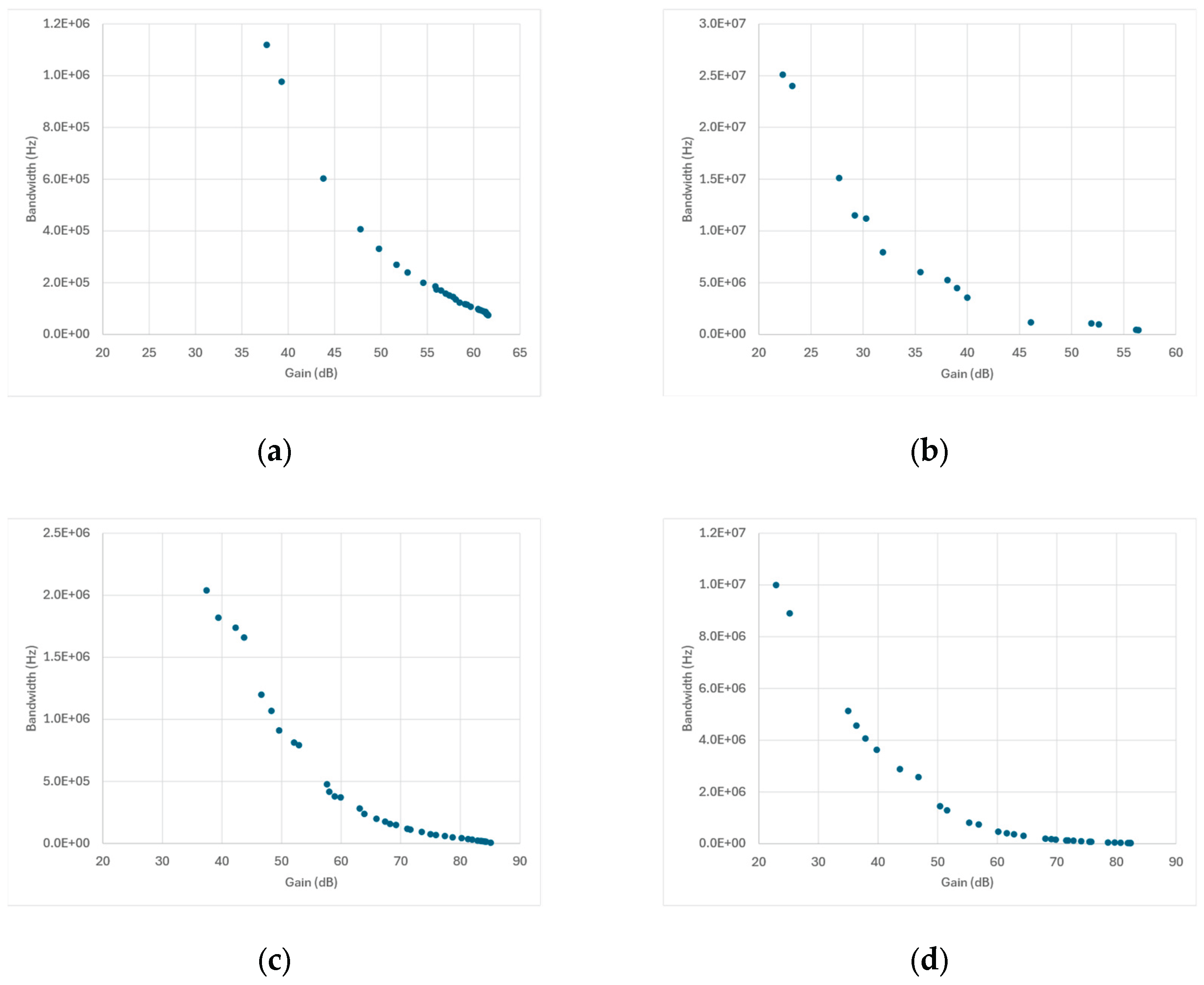
The MOEA/D configuration used in this work was selected primarily to ensure fair comparison with the other optimization algorithms (NSGA-II, NSGA-III, and SPEA2). For consistency, analogous settings were adopted across all methods—namely, a population size of 100 (corresponding to 100 subproblems in MOEA/D), a crossover probability of 0.9, a mutation probability of 0.1, and a similar early-stopping criterion (see Table 2). This common configuration allowed a balanced assessment of simulator performance under equivalent computational workloads and solver conditions, including identical SPICE analysis parameters and solver tolerances.
Under these settings, the Pareto fronts generated by MOEA/D exhibited the expected gain–bandwidth trade-off but showed a sparser solution distribution, with most non-dominated points clustered toward the high-gain region. This outcome reflects our conservative configuration biased toward fast local convergence rather than broad design-space exploration. Specifically, the combination of high crossover probability, low mutation rate, and strong parent-selection locality (delta = 0.9, neighbors = 15) emphasizes exploitation over exploration. The Tchebycheff decomposition further reinforces this tendency by driving optimization toward extreme objective values. Namely, Tchebycheff decomposition tends to favor the objective that is easier to improve—in this case, gain—so the search mostly converges toward high-gain regions while exploring the low-gain, high-bandwidth trade-offs less extensively.
Table 4 shows the summary of MOEA/D optimization statistics using sequential execution. All MOEA/D simulations processed 5000 design evaluations (50 iterations over 100 individuals) under identical optimization and SPICE-solver conditions.
The transistor-compensated differential amplifier exhibits the highest cache-reuse ratio (≈ 91%), confirming strong convergence toward a limited set of recurring designs. However, its throughput remains low (≈ 6.5 sim/s) because frequent database lookups dominate runtime once cache hits prevail. The other amplifier topologies show similar cache-hit levels (≈ 70–74%) and slightly higher throughputs of 9–13 sim/s, consistent with a more balanced mix of cached and new evaluations.
Despite exploiting PyMoo’s internal parallel-evaluation backend, the results summarized in Table 5 indicate that parallel execution does not yield any measurable performance improvement over the sequential MOEA/D runs. Across all amplifier topologies, the wall-clock times remain comparable or even slightly higher, confirming that the internal thread-level parallelism introduces additional scheduling and synchronization overhead that offsets the potential benefit of concurrent SPICE evaluations.
The throughput values (≈ 5–13 sim/s) are effectively identical to those of the sequential configuration, demonstrating that evaluation latency is dominated by SPICE solver execution and cache I/O rather than CPU availability. Similarly, the cache-hit ratios remain in the 0.68–0.77 range (and 0.93 for the transistor-compensated amplifier), showing that parallelization neither enhances design reuse nor affects the caching dynamics established by MOEA/D’s decomposition-based search. These results confirm that, on a single-machine setup, PyMoo’s internal parallelization provides no runtime benefit compared with sequential execution, as the optimization remains constrained by SPICE simulation cost and I/O-bound cache operations rather than computational parallelism.
3.3.2. Surrogate-Guided Optimization
The surrogate-guided optimization (SGO) strategy was also employed to accelerate the multiobjective analog circuit design process by coupling machine-learning-based surrogate models with periodic SPICE truth evaluations. In the adopted configuration, the optimization proceeded with a truth interval of two generations—meaning that every two evolutionary generations, the surrogate model was updated and validated against ground-truth SPICE simulations. Each verification stage (truth sweep) comprised a truth batch size of 16, corresponding to the number of candidate designs selected by the surrogate for SPICE evaluation in each update cycle. As a result, only 3.5% of all evaluated individuals were subjected to full SPICE simulation, while 96.5% of evaluations relied on fast surrogate inferences. This hybrid approach drastically reduced the computational burden, yielding an approximate 94% reduction in total simulation time compared to pure SPICE-based optimization.
Surrogate predictions were deliberately not parallelized because they already execute as highly efficient, batched vector operations that fully exploit optimized numerical kernels on the CPU. In this context, the computational asymmetry between model inference and circuit-level SPICE evaluations is extreme—predictions are orders of magnitude faster, so distributing them across multiple processes would introduce overheads that outweigh any potential gains. Batched inference ensures optimal use of CPU vector units and system memory without duplicating model parameters across processes, while avoiding thread contention and preserving deterministic numerical behavior essential for reproducibility in evolutionary loops. Consequently, parallel execution was applied only to the high-latency SPICE truth evaluations, where it brings tangible benefits provided that the batch size is sufficiently large—but not in this case, where the truth batch represented a small fraction of the overall workload. Under these conditions, only surrogate model training benefits meaningfully from parallelization, while inference remains an in-process, vectorized operation that is both simpler and more stable on a CPU-only system. As a result, parallel execution provided no significant additional speedup, and comparable runtimes were observed across all genetic algorithms under test.
The performance of the surrogate-guided optimization (SGO) process was assessed by jointly analyzing the quality of the resulting Pareto fronts and the predictive accuracy of the surrogate models. The Pareto front evaluation provides a direct measure of how effectively the SGO strategy captures the trade-off surface between conflicting design objectives, revealing whether the surrogate-driven exploration converges toward the true multiobjective optimum identified by SPICE ground-truth evaluations. Complementarily, the predictive performance of the surrogate models was quantified using the Mean Absolute Error (MAE) computed over each truth batch.
MAE was selected as the principal accuracy metric for several reasons directly aligned with the dynamics of surrogate-assisted optimization. First, it offers direct interpretability in the same units as the design objectives (e.g., dB for gain, Hz for bandwidth), allowing engineers to immediately assess the average prediction deviation without requiring squaring or square-root transformations as in MSE or RMSE. This makes MAE particularly useful for adaptive control of surrogate updates, such as checkpoint acceptance and rollback decisions during the optimization loop.
Second, MAE exhibits robustness to outliers, which are common in analog circuit design where certain candidates may produce invalid or unstable operating points. Unlike MSE, which amplifies large errors quadratically and can distort model assessment, MAE treats all deviations linearly, ensuring that a few extreme mispredictions do not overshadow the typical predictive behavior across the Pareto front. This stability translates into more reliable model update and rollback logic.
Third, MAE provides consistent scaling across multiple objectives with heterogeneous numerical ranges—such as gain (20–100 dB) and bandwidth (10³–10⁹ Hz) —without biasing the aggregate error toward high-magnitude variables. The metric also produces a stable and predictable convergence signal: thresholds like rollback if MAE increases by > 0.15 can be tuned intuitively because MAE’s scale remains bounded and insensitive to isolated large errors.
Finally, MAE is computationally efficient and empirically validated in our workflow. It requires only the sign of the residual during backpropagation, reducing numerical overhead and improving stability during online surrogate updates. In practice, the MAE exhibits a generally decreasing trend as the number of generations increases, showing an oscillatory behavior that reflects the adaptive refinement of the surrogate model through successive truth evaluations. This evolution indicates progressive improvement in predictive accuracy and stability, further confirming the effectiveness of the adopted SGO strategy.
The Pareto fronts presented in Figure 15 confirm that surrogate-guided optimization effectively captures the trade-off between gain and bandwidth across all amplifier topologies, producing fronts consistent with the expected hyperbolic trend observed in pure SPICE-based optimization. For the Miller- and telescopic-cascode amplifiers, the predicted fronts show good coverage of the of the objective space with a coherent, monotonic profile—consistent with well-behaved surrogate generalization. The folded-cascode case exhibits a similar overall quality, with the notable exception of a slight clustering in the high-gain / low-bandwidth region, indicating local over-exploitation of that corner of the trade-off.
A topology–algorithm interaction emerges for the transistor-compensated differential amplifier under SPEA2 (see Figure 15f). Post-analysis of the surrogate inference logs revealed that, in this case, the surrogate performed a large number of redundant predictions—assigning identical output metrics to multiple distinct design vectors which led to overlapping points and a degraded Pareto front. This redundancy is compatible with a training set locally saturated in similar samples and with SPEA2’s archive dynamics, which can preserve minimally distinct individuals once dominance relations stabilize. By contrast, NSGA-II and NSGA-III—through crowding and reference-direction mechanisms—are less susceptible to this collapse and yield more evenly distributed predicted fronts.
These observations underscore the need to periodically re-enrich the surrogate with diverse ground-truth samples (e.g., targeted truth checks in sparsely populated regions) and to monitor prediction uniqueness to prevent accumulation of duplicates, especially for archive-based algorithms and topologies prone to local clustering.
The MAE trends in Figure 16 confirm that, in most cases, surrogate accuracy improves progressively with successive ground-truth updates, following the expected pattern of oscillatory but overall decreasing error. For the Miller-compensated amplifier, NSGA-II shows a rapid drop in MAE that stabilizes early at a low error level, whereas SPEA2exhibits steadier oscillations with a slower but continuous decline. NSGA-III, instead, presents wider fluctuations, indicating stronger corrective adjustments as the optimizer compensates for larger initial prediction discrepancies. In contrast, the folded-cascode amplifier displays a smoother downward trend across all algorithms, reaching consistently low MAE values that reflect stable convergence and effective surrogate refinement.
The telescopic-cascode amplifier follows a similar overall behavior but with more irregular fluctuations. This pattern likely arises from the amplifier’s higher sensitivity to device-level parameter interactions which amplify small modeling inaccuracies and cause local prediction corrections to vary more strongly between truth batches.
Figure 15.
Pareto fronts obtained through surrogate-guided optimization (SGO) for the different amplifier topologies and genetic algorithms under test (NSGA-II, NSGA-III, and SPEA2, respectively). The explored design space is and : (a-c) Miller-compensated differential amplifier; (d-f) Transistor-compensated differential amplifier; (g-i) folded-cascode op-amp; (l-n) Telescopic-cascode amplifier.
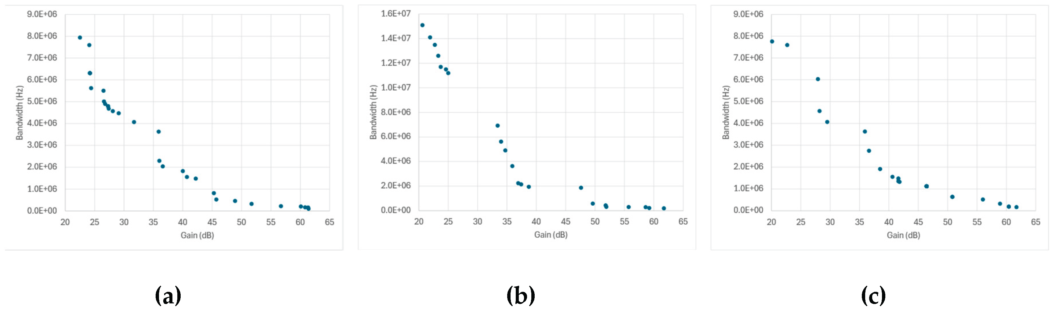
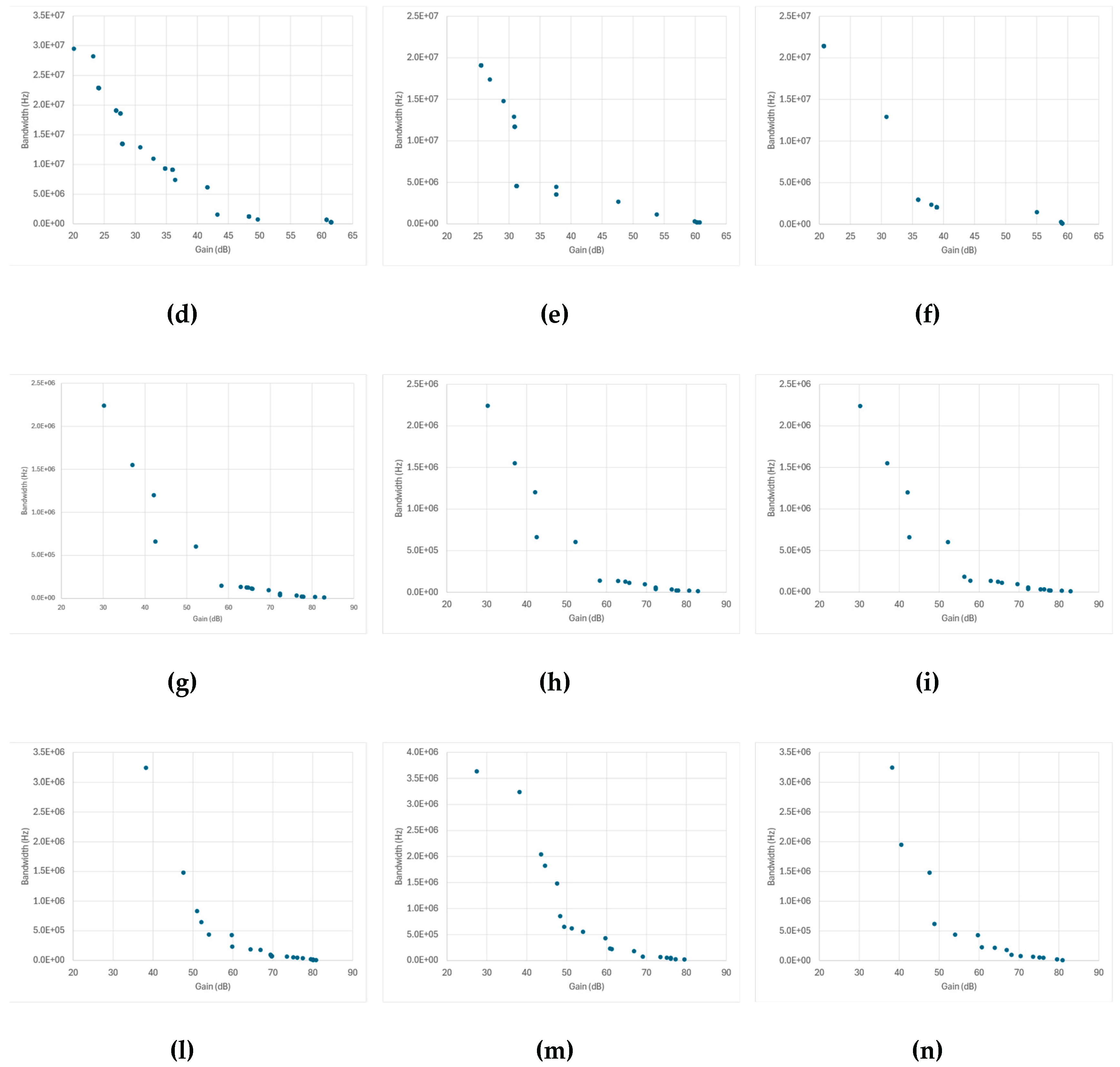
A distinctive behavior is observed for the transistor-compensated differential amplifier, where all three algorithms show a monotonic decrease of MAE with generation, comparable to the other topologies. This confirms that, despite the poor Pareto front observed for this case with SPEA2, the surrogate predictions remain accurate overall. The degradation in the Pareto front thus stems not from high prediction error, but from redundant surrogate outputs, where distinct input parameter combinations yield identical gain and bandwidth values. Such redundancy limits design diversity but does not compromise the surrogate’s numerical accuracy, which continues to improve steadily across generations.
The oscillatory but steadily declining MAE curves validate the soundness of the SGO workflow and demonstrate that the surrogate maintains effective predictive accuracy across generations, with local variations arising mainly from topology-dependent model complexity and algorithmic sampling diversity.
Figure 16.
Evolution of the Mean Absolute Error (MAE) of the surrogate model during surrogate-guided optimization (SGO) for the four amplifier topologies under study. Curves report MAE values versus truth batch index for NSGA-II, NSGA-III, and SPEA2, averaged over all predicted individuals per generation (ground-truth evaluations are performed every two generations to update the surrogate and measure prediction accuracy). Each plot corresponds to: (a) Miller-compensated differential amplifier; (b) Transistor-compensated differential amplifier; (c) folded-cascode op-amp; (d) Telescopic-cascode amplifier.
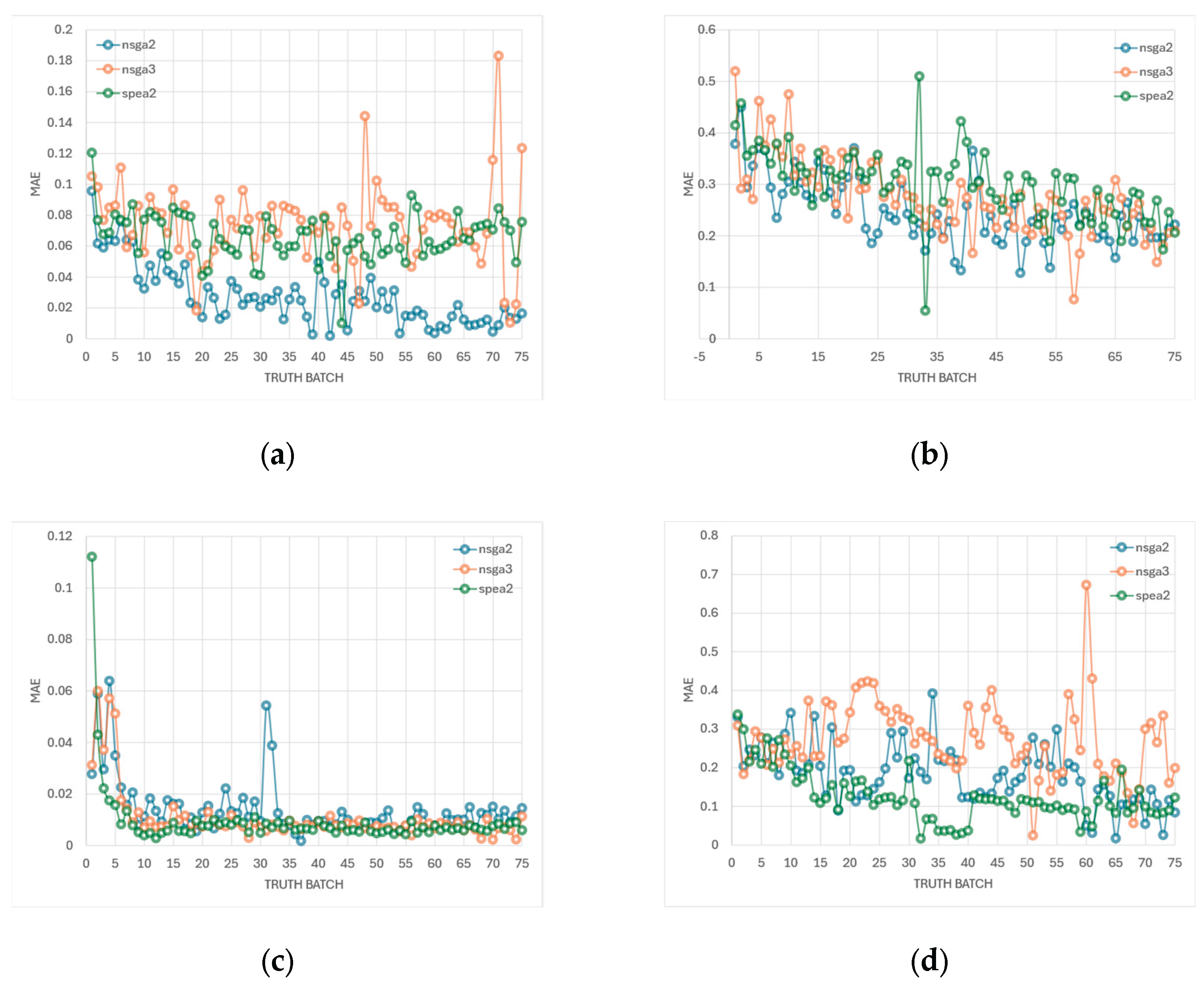
Finally, Table 6 complements the MAE-evolution analysis by providing quantitative statistics over 12 independent SGO runs for each amplifier topology. The results confirm the overall improvement in surrogate accuracy observed in Figure 16, with the MAE consistently decreasing between the initial, final, and best-recorded values across all designs. The folded-cascode amplifier achieves the lowest median final MAE (≈ 0.022), reflecting its smoother response surface and higher predictability. The Miller-compensated amplifier follows closely, although the wider range between runs indicates moderate sensitivity to the specific training trajectory. The telescopic-cascode amplifier maintains a clear reduction in MAE but with larger residual errors, consistent with its more complex biasing and coupling behavior. The transistor-compensated differential amplifier remains the most challenging case, exhibiting the highest initial and final MAEs, yet still demonstrating a consistent downward trend.
3.3.3. Multi-Fidelity Adaptive Optimization
While surrogate-guided optimization (SGO) relies on a fixed verification schedule with periodic ground-truth batches evaluated at constant intervals, multi-fidelity optimization (MFO) introduces a dynamic fidelity allocation strategy that adapts evaluation effort based on real-time uncertainty quantification. The key distinction lies in the decision process: SGO verifies a predetermined fraction of candidates using SPICE at regular generational intervals, whereas MFO employs an adaptive fidelity controller that assigns high-fidelity evaluations to selected candidates according to composite scoring criteria—such as uncertainty-driven, hybrid exploitation–exploration, or hypervolume-proxy strategies.
This adaptive scheme is complemented by an uncertainty penalty mechanism that continuously adjusts the penalty weight applied to surrogate predictions in proportion to the current mean uncertainty relative to a predefined target value. When the global uncertainty exceeds this threshold, the penalty weight increases, discouraging exploration in regions of low surrogate confidence; conversely, when the uncertainty falls below the target, the penalty is relaxed, enabling broader exploration of the design space.
Through this closed-loop adaptation, MFO automatically balances computational cost and prediction confidence throughout the optimization process. This makes it particularly effective for problems where the surrogate’s reliability is non-uniform across the design space or evolves as additional ground-truth data are incorporated. The defining feature of MFO is therefore the shift from a schedule-based verification policy to a confidence-based allocation of computational resources, allowing SPICE evaluations to focus where the surrogate is least reliable while sustaining aggressive exploration in well-modeled regions. The Pareto fronts in Figure 16 demonstrate that multi-fidelity optimization successfully enhances the consistency and smoothness of the predicted trade-offs between gain and bandwidth compared with the fixed-interval surrogate-guided approach. Across all amplifier topologies, MFO produces denser and more uniformly distributed Pareto fronts, indicating that adaptive fidelity allocation effectively concentrates high-fidelity evaluations in regions where the surrogate’s uncertainty is higher, while relying on low-fidelity inference in well-modeled areas.
Figure 16.
Pareto fronts obtained through multi-fidelity optimization (MFO) for the different amplifier topologies and genetic algorithms under test (NSGA-II, NSGA-III, and SPEA2, respectively). The explored design space is and : (a-c) Miller-compensated differential amplifier; (d-f) Transistor-compensated differential amplifier; (g-i) folded-cascode op-amp; (l-n) Telescopic-cascode amplifier.
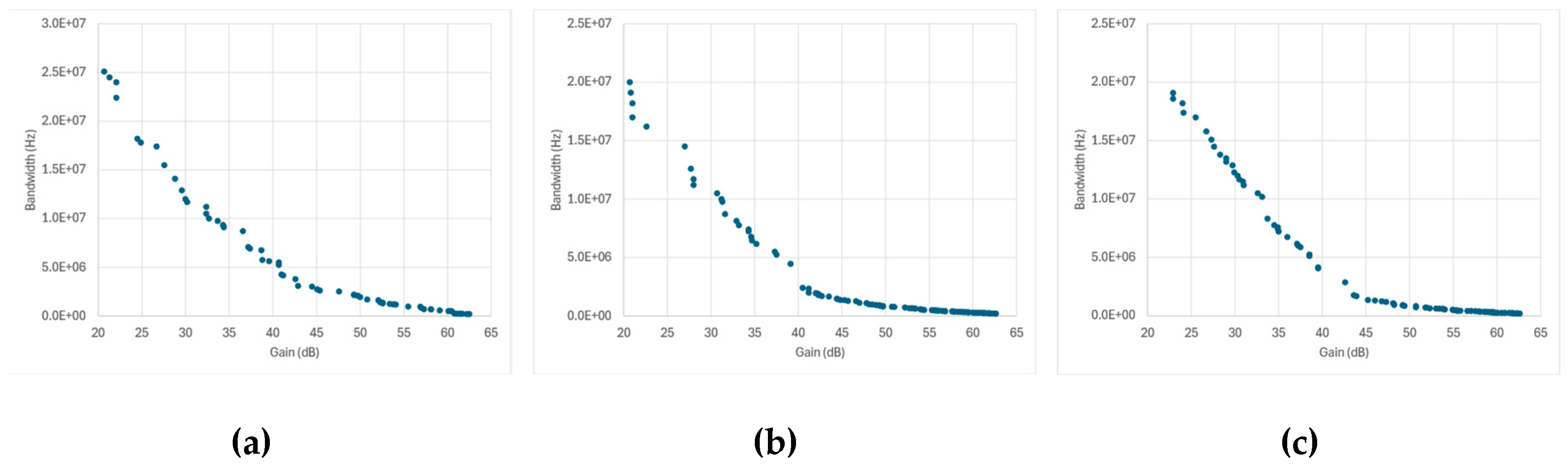
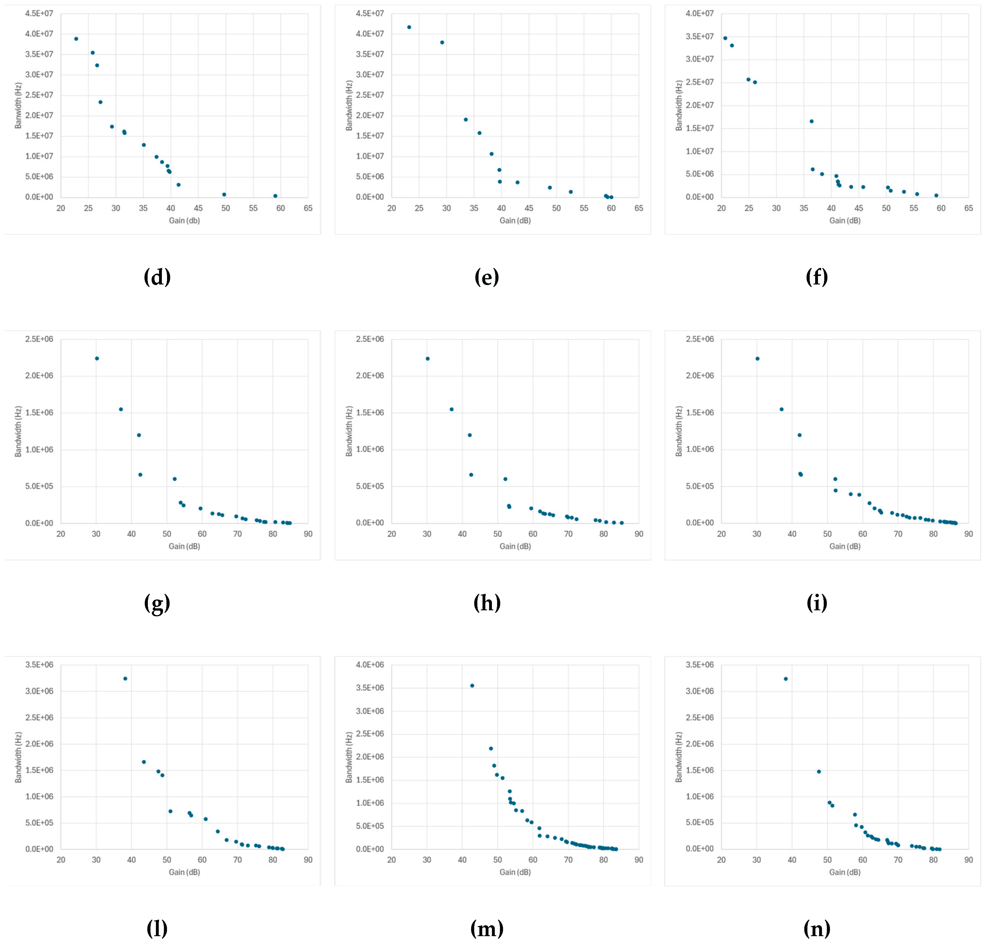
For the Miller-compensated and folded-cascode amplifiers, all three algorithms converge to well-defined, continuous fronts that closely approximate the expected monotonic gain–bandwidth relation. The improvement over the single-fidelity surrogate-guided optimization is particularly evident in the edge regions of the Pareto front, where MFO avoids the local sparsity previously observed due to fixed truth intervals.
The telescopic-cascode amplifier also benefits from the adaptive scheme, showing a more stable front with fewer scattered or discontinuous points. This suggests that MFO’s uncertainty-driven truth allocation efficiently mitigates the effects of local nonlinearity and parameter coupling that previously introduced variability in surrogate-only predictions. A notable improvement is seen in the transistor-compensated differential amplifier, especially for SPEA2, where the degenerate Pareto front observed in the surrogate-guided case is now replaced by a more evenly spread set of trade-off solutions. The adaptive uncertainty controller in MFO selectively reinforces ground-truth verification for individuals exhibiting high predictive variance, thus breaking the redundancy that led to overlapping predictions in the previous configuration.
The multi-fidelity optimization framework monitors two key uncertainty metrics to guide the adaptive allocation of high-fidelity SPICE simulations: UncMean (mean predicted uncertainty across the population) and UncP95 (95th percentile uncertainty). These metrics quantify the surrogate model’s confidence in its predictions, with lower values indicating higher reliability.
The fidelity allocation mechanism employs a composite scoring approach rather than simple threshold-based selection. While the system uses an initial uncertainty threshold of 0.15 to flag candidates potentially requiring SPICE verification, the actual selection is rank-based: candidates are scored using normalized uncertainty combined with exploitation or diversity metrics (depending on the acquisition strategy), and the top-N are allocated for SPICE evaluation. The simulator has been configured so that the target SPICE fraction is adaptively adjusted between 10% and 30% of the population based on the proportion of candidates exceeding the threshold. To prevent excessive reliance on uncertain predictions, the framework includes an adaptive penalty mechanism that targets a mean uncertainty of 0.3. When UncMean exceeds this target, a penalty weight is gradually increased (default adaptation rate: 0.15 per generation, maximum weight: 2.0), adding a penalty term proportional to prediction uncertainty to the objective function. This encourages the optimizer to explore regions where the surrogate is more confident. Conversely, when UncMean falls below the target, the penalty decreases.
In our experiments across four op-amp topologies, uncertainty metrics remained consistently well below both thresholds (UncMean < 0.15, UncP95 < 0.15), indicating excellent surrogate quality throughout optimization. This resulted in penalty weights remaining near zero and enabled sustained high surrogate reliance (89.7% of evaluations) without sacrificing prediction reliability. However, consistently low uncertainty from the start raises important considerations regarding potential optimization bias. When the surrogate maintains high confidence early in the search, there is a risk of premature convergence through: (1) over-exploitation of known regions, where the optimizer preferentially samples areas of existing confidence rather than exploring uncertain regions; (2) false confidence, where low uncertainty does not guarantee accuracy—the model may be confidently incorrect in unexplored areas, leading to locally optimal but globally suboptimal Pareto fronts; (3) reduced diversity, as minimal SPICE verification (10% at minimum allocation) provides limited opportunity to detect missing design space features; and (4) initial training bias, where DOE samples concentrated in specific regions produce surrogates that are well-trained locally but ignorant yet falsely confident in undersampled areas.
Figure 17.
Evolution of the batch uncertainty during multi-fidelity optimization (MFO) for the different amplifier topologies and genetic algorithms under test (NSGA-II, NSGA-III, and SPEA2, respectively): (a-c) Miller-compensated differential amplifier; (d-f) Transistor-compensated differential amplifier; (g-i) folded-cascode op-amp; (l-n) Telescopic-cascode amplifier.
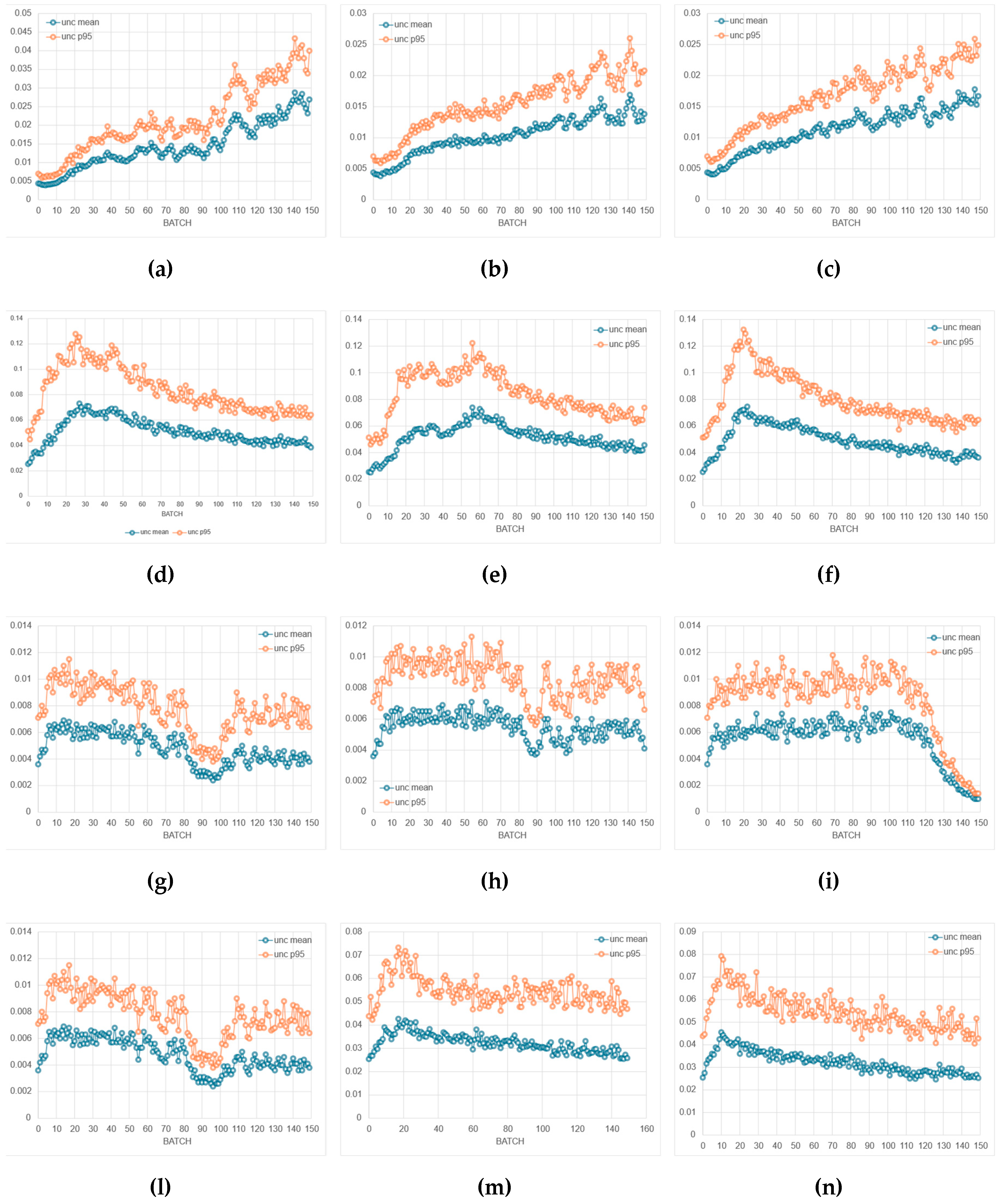
Empirical analysis across our runs revealed a robust correlation between uncertainty evolution and Pareto quality: runs achieving the best Pareto fronts consistently exhibited monotonically increasing UncMean and UncP95, indicating sustained exploration into previously unseen regions of the design space as superior trade-offs were discovered. Conversely, runs with stationary or monotonically decreasing uncertainty tended to stagnate and produced inferior fronts, consistent with premature convergence and over-exploitation of already-confident regions.
Importantly, this pattern held across multiple MOEAs—including NSGA-II, NSGA-III, and SPEA2—suggesting it is not tied to a specific algorithmic detail but rather to a general exploration–exploitation dynamic. As the search moves toward novel objective combinations and parameter regimes, the surrogate naturally encounters unfamiliar inputs, which increases predictive uncertainty; in this context, rising uncertainty is a healthy signal of active exploration rather than model degradation.
These dynamics are supported by the framework’s diversity-preserving mechanisms (e.g., niching and reference-point guidance in NSGA variants, strength-based selection in SPEA2), the composite scoring used for fidelity allocation (which blends uncertainty with exploitation/diversity cues), the hypervolume-proxy option that explicitly rewards frontier expansion, and continuous retraining from SPICE-verified samples. Together, these elements mitigate exploitation bias while enabling the surrogate to remain the dominant evaluator without sacrificing discovery.
The aggregated MAE convergence data in Table 7 confirm that the surrogate models consistently improve their predictive accuracy throughout the optimization process. The mean relative improvement ranges between approximately 40% and 65%, depending on the circuit topology, with the folded-cascode and Miller-compensated amplifiers showing the strongest refinement. Conversely, the transistor-compensated differential amplifier and the telescopic-cascode amplifier remain the most challenging cases, exhibiting smaller MAE reductions and higher final residual errors. These results are consistent with their more irregular Pareto fronts and the stronger parameter coupling expected in these topologies, which complicate accurate surrogate interpolation.
When these MAE dynamics are cross-referenced with the uncertainty-evolution trends, a consistent pattern emerges. Runs achieving the best Pareto fronts are not necessarily those with the lowest final MAE, but rather those exhibiting increasing uncertainty throughout the optimization trajectory. This correlation indicates that uncertainty growth serves as an indicator of active exploration, as the optimizer encounters novel regions of the design space where the surrogate confidence is lower.
In contrast, runs with flat or decreasing uncertainty curves—particularly those associated with limited MAE improvement—tend to converge in suboptimal regions, leading to poorer trade-offs. Thus, while decreasing MAE confirms the surrogate’s improving reliability, maintaining a moderate level of predictive uncertainty is essential to preserve exploration pressure and prevent the optimizer from over-exploiting already well-characterized regions.
Figure 18 reports the average wall-clock time per generation for both sequential and parallel multi-fidelity optimization (MFO) runs for all the amplifier topologies and genetic algorithms under test. The per-generation timing profiles presented in Figure 18 provide a qualitative view of the temporal evolution of the optimization process and highlight the impact of parallel execution on runtime stability.
To complement these observations with quantitative data, Table 8 summarizes the corresponding average wall-clock times and parallel execution metrics for all amplifier topologies and algorithms. This table consolidates the results across both sequential and parallel configurations, allowing a direct assessment of overall speedups, efficiency, and time reduction achieved by the multi-fidelity optimization framework under identical solver and uncertainty-control settings.
The wall-clock time evolution per generation across all multi-fidelity optimization runs reveals distinct performance profiles for different amplifier topologies and genetic algorithms. On average, sequential execution exhibits generation times ranging from 0.7 to 1.3 seconds per generation, with folded cascode showing the shortest execution times (0.8 s/gen) and transistor-compensated differential amplifier requiring the longest (1.3 s/gen). Parallel execution with multiple workers yields substantial performance improvements, achieving an average speedup of 2.54× and reducing total wall-clock time by approximately 60.2% on average. The parallel efficiency averages 31.7%, indicating limited scaling behavior. The deviation from ideal linear speedup can be attributed to synchronization overhead in batch-based SPICE evaluations and the inherent sequential dependencies in adaptive surrogate model updates.
4. Discussion
This section synthesizes the main findings presented in Section 3 and focuses on strategies to improve both the quality of the simulation results and the runtime performance of the proposed framework.
4.1. Summary of Key Observations
Surrogate-Guided Optimization (SGO) produced Pareto fronts consistent with the SPICE truth evaluations while achieving progressively higher predictive accuracy. The Mean Absolute Error (MAE) followed an oscillatory but overall decreasing trajectory across successive truth batches, confirming the effectiveness of the update and rollback governance adopted for SGO (Section 3.3). In the experiments reported here, truth updates were performed every two generations with a batch size of 16 individuals, selected through a combination of uncertainty-aware and diversity-based sampling strategies.
In Multi-Fidelity Optimization (MFO), the average wall-clock time per generation was markedly reduced through parallel SPICE execution. On a single machine with 8 workers, process-based parallelism systematically outperformed sequential execution, achieving typical speedups of 2.0–3.0× (mean: 2.54×, range: 2.04–2.95×) averaged across amplifier topologies and algorithms, with an average parallel efficiency of 31.7%. In cache-dominated regimes—where hit rates exceeded 85% in later generations—the relative contribution of I/O overhead becomes more pronounced, potentially limiting further speedup gains despite shorter computational times. This effect was particularly evident in the transistor-compensated amplifier topology, where high cache utilization resulted in diminishing returns from parallelization.
For MOEA/D, the Pareto fronts appeared sparser and biased toward high-gain solutions under the “fair-comparison” configuration. This behavior is consistent with the Tchebycheff decomposition (with δ=0.9 and 15 neighbors) employed, which tends to favor exploitation over exploration in the localized mating neighborhood (Section 3.3.1).
4.2. Improving Result Quality
4.2.1. Algorithm-Specific Tuning
A uniform genetic-operator configuration (crossover probability 0.9, mutation probability 0.1) was adopted across all algorithms to guarantee fair benchmarking; however, algorithm-specific tuning could improve convergence and front coverage. In particular, MOEA/D could benefit from reduced locality (lower δ or fewer neighbors) or alternative decomposition methods (PBI or weighted-sum) to achieve better solution spread. SPEA2 could benefit from stricter duplicate filtering and more pressure-sensitive archive management, while NSGA-III could refine the density of its reference directions to improve distribution in two-objective problems. These adjustments directly address the sparsity observed in MOEA/D and the duplicate-prediction sensitivity noted in SPEA2’s archive dynamics.
4.2.2. Adaptive Data Enrichment
When clustering or redundant surrogate predictions occur, the existing diversity-aware truth selection strategies (greedy farthest-point sampling or crowding distance-based selection) help mitigate this issue by prioritizing geometrically diverse candidates. However, explicitly monitoring prediction uniqueness alongside MAE—triggering targeted re-enrichment in sparse regions when identical outputs are generated from distinct input vectors—could further improve diversity without increasing the overall truth budget. This would complement the current uncertainty-driven selection with explicit redundancy detection.
4.2.3. Verification Cadence and Batch Size
The fixed SGO verification schedule (truth updates every two generations with a batch size of 16) performed effectively overall, but adaptive scheduling may yield further improvements. Increasing the batch size when MAE plateaus, or shortening the truth interval during rapid Pareto expansion, could reduce local bias and accelerate convergence without significantly increasing computational cost. Dynamic adjustment of verification frequency based on observed surrogate drift would allow the framework to balance exploration and exploitation more efficiently.
4.3. Improving Runtime Performance
4.3.1. Process-Based Parallelism
The results demonstrate that process-based parallel execution consistently achieves lower wall-clock times than sequential execution on single-host configurations. The framework leverages process-pool parallelism for both population evaluations and high-fidelity verification batches in MFO, with automatic backend selection favoring process spawning over distributed schedulers for single-machine deployments. On the tested hardware, this approach delivered robust performance gains across all topologies and algorithms.
4.3.2. Mitigating I/O Bottlenecks
In cache-heavy runs, performance becomes increasingly I/O-bound rather than compute-bound. The current implementation employs SQLite with Write-Ahead Logging (WAL) mode, NORMAL synchronization, and appropriate timeout handling to support concurrent access. To further alleviate I/O limitations—particularly in high-throughput scenarios—additional optimizations could include explicit transaction batching (grouping multiple writes into single commits), tuning SQLite’s cache_size pragma for larger in-memory buffers, and implementing more aggressive index strategies for frequently queried columns. These refinements would complement the existing hybrid in-memory and SQLite cache architecture (Section 2) and address the flat throughput trends observed despite shorter wall times.
4.3.3. Inference Optimization
Both population evaluations and high-fidelity verification batches in MFO leverage parallel execution when configured with multiple workers, as reflected in the speedup measurements reported in Section 3. Since surrogate inference remains orders of magnitude faster than SPICE simulation and operates efficiently with vectorized in-process evaluation, maintaining inference as a vectorized operation without distributed overhead is appropriate. The observed parallel efficiencies (averaging 31.7%) primarily reflect SPICE evaluation overhead and synchronization costs rather than inference bottlenecks.
4.4. Overall Assessment
The analysis presented in Section 3 indicates that simulation accuracy is governed primarily by careful truth-checking, diversity management, and adaptive sampling—reflected in steadily declining MAE across generations—whereas runtime performance is dictated mainly by SPICE parallelism and cache I/O throughput. Under the uniform configuration used for fairness, algorithmic choice exerts only a secondary influence on average wall-clock performance; per-generation time variation across algorithms (0.26–0.43 s) is smaller than variation across topologies (folded_cascode: 0.26–0.31 s; transistor_comp: 0.39–0.43 s). Consequently, future refinements should concentrate on algorithm-specific configuration tuning, adaptive verification scheduling, and I/O optimization to enhance both front quality and computational efficiency.
5. Conclusions
This study compared SPICE-only, Surrogate-Guided (SGO), and Multi-Fidelity Optimization (MFO) strategies across several amplifier topologies using NSGA-II, NSGA-III, SPEA2, and MOEA/D under a uniform configuration to ensure fairness. The results confirm that surrogate-based workflows substantially reduce computational cost while maintaining close agreement with SPICE truth.
Table 9 summarizes the main characteristics and trade-offs among the three optimization modes. SPICE-only evaluation guarantees perfect accuracy but at the highest computational cost. SGO achieves the largest speedup by replacing most evaluations with surrogate predictions, while MFO introduces adaptive verification to sustain accuracy with moderate additional cost.
Under identical solver and population settings, process-based parallelism yielded the most efficient runtime (≈ 2–3× speedup) while preserving surrogate accuracy; cluster-based scheduling introduced additional overhead without improving throughput. Accuracy improvements were topology-dependent: the folded-cascode amplifier consistently reached the lowest MAE, while transistor-compensated and telescopic-cascode designs remained more challenging due to stronger parameter coupling.
To conclude, surrogate-assisted optimization offers a practical compromise between accuracy and computational efficiency. Future work will relax the uniform-configuration constraint to enable algorithm-specific tuning, improve cache and I/O performance, and extend adaptive parallelism to high-fidelity verifications—steps expected to further enhance both result quality and runtime scalability without altering the overall framework.
Supplementary Materials
The supplementary materials are available at: https://doi.org/10.5281/zenodo.17503736. Dataset (simulation_data_v1.0.zip): Simulation outputs generated by the simulator presented in this paper and companion documentation describing the data lake structure and implementation details.
Author Contributions
Conceptualization, G.C., A.T., J.C. and A.Z.; methodology, G.C., A.T., J.C. and A.Z.; software, G.C.; validation, J.C., A.T. and A.Z.; formal analysis, G.C., A.T., J.C. and A.Z; investigation, G.C., A.T., J.C. and A.Z.; writing—original draft preparation, G.C.; writing—review and editing, G.C., A.T., J.C. and A.Z All authors have read and agreed to the published version of the manuscript.
Funding
This research received no external funding.
Data Availability Statement
All methodological details necessary to permit independent reimplementation are provided in the manuscript (algorithms, metrics, optimization procedures, and evaluation protocols). Due to pending IP transfer, the original source code is not publicly archived. Aggregated benchmark results and derived performance metrics used in the figures can be provided upon reasonable academic request, subject to intellectual property constraints. Exceptionally, and under a non-disclosure agreement, a binary artifact or redacted implementation may be shared only for verification purposes upon reasonable request until commercialization milestones are complete.
Acknowledgments
During the preparation of this manuscript, the authors used ChatGPT v5.0 and Microsoft Word Copilot to debug code, improve the English, punctuation, and overall paper structure, to conduct bibliographic research, to analyze and summarize bibliographic references, and to check for possible research overlaps with other authors. The authors have carefully reviewed and edited the output and take full responsibility for the content of this publication.
Conflicts of Interest
G. C. is the sole developer of the software described and is in the process of assigning all rights to Helianthus Technologies for prospective commercial exploitation. Consequently, the full source code and certain implementation artifacts cannot be made publicly available at this time. Apart from the forthcoming commercial assignment noted above, the authors declare no other conflicts of interest.
Abbreviations
The following abbreviations are used in this manuscript:
| AST | Abstract Syntax Tree |
| BO | Bayesian Optimization |
| CDF | Cumulative Distribution Function |
| CLI | Comman Line Interface |
| DoE | Design of Experiments |
| DSL | Domain Specific Language |
| DUT | Device Under Test |
| EA | Evolutionary Algorithm |
| EBNF | Extended Bakus-Naur Form |
| EI | Expected IMprovement |
| GA | Genetic Algorithm |
| GAT | Graph Attention Layer |
| GCN | Graph Convolutional Network |
| GNN | Graph Neural Network |
| GP | Gaussian Process |
| HF | High Fidelity |
| HPO | Hyperparameters Optimization |
| HV | Hypervolume |
| IGD | Inverted Generational Distance |
| LHS | Latin Hypercube Sampling |
| LF | Low Fidelity |
| ML | Machine Learning |
| MLP | Multilayer Perceptron |
| MOEA | Multiobjective Evolutionary Algorithm |
| MOEA/D | Multiobjective Evolutionary Algorithm based on Decomposition |
| MSM | Multi-fidelity Surrogate Model |
| NSGA-II/-III | Non-dominated Sorting Genetic Algorithm II/III |
| Probability Density Function | |
| RBF | Radial Basis Function |
| RF | Random Forest |
| SAEA | Surrogate-assisted Evolutionary Algorithm |
| SAO | Surrogate-assisted Optimization |
| SBX | Simulated Binary Crossover |
| SPEA2 | Strength Pareto Evolutionary Algorithm 2 |
| TTL | Time To Live |
References
- Deb, K.; Pratap, A.; Agarwal, S.; Meyarivan, T. A Fast and Elitist Multiobjective Genetic Algorithm: NSGA-II. IEEE Trans. Evol. Comput. 2002, 6, 182–197. [CrossRef]
- Zitzler, E.; Thiele, L.; Laumanns, M.; Fonseca, C.M.; da Fonseca, V.G. Performance Assessment of Multiobjective Optimizers: An Analysis and Review. IEEE Trans. Evol. Comput. 2003, 7, 117–132. [CrossRef]
- Liu, S.; Wang, H.; Peng, W. Surrogate-Assisted Evolutionary Algorithms for Expensive Combinatorial Optimization: A Survey. Complex Intell. Syst. 2024, 10, 5933–5949. [CrossRef]
- Yu, H.; Gong, Y.; Kang, L.; et al. Dual-Drive Collaboration Surrogate-Assisted Evolutionary Algorithm by Coupling Feature Reduction and Reconstruction. Complex Intell. Syst. 2024, 10, 171–191. [CrossRef]
- Chugh, T.; Rahat, A.; Volz, V.; Zaefferer, M. Towards Better Integration of Surrogate Models and Optimizers. In High-Performance Simulation-Based Optimization; Bartz-Beielstein, T., Filipič, B., Korošec, P., Talbi, E.G., Eds.; Studies in Computational Intelligence; Springer: Cham, Switzerland, 2020; Volume 833, pp. 119–139. [CrossRef]
- Jin, Y. Surrogate-Assisted Evolutionary Computation: Recent Advances and Future Challenges. Swarm Evol. Comput. 2011, 1, 61–70. [CrossRef]
- Ruan, X.; Li, K.; Derbel, B.; Liefooghe, A. Surrogate Assisted Evolutionary Algorithm for Medium Scale Multi-Objective Optimisation Problems. In Proceedings of the 2020 Genetic and Evolutionary Computation Conference (GECCO ‘20), New York, NY, USA, 8–12 July 2020; pp. 560–568. [CrossRef]
- Zhang, S.; Lyu, W.; Yang, F.; Yan, C.; Zhou, D.; Zeng, X. Bayesian Optimization Approach for Analog Circuit Synthesis Using Neural Network. In Proceedings of the 2019 Design, Automation & Test in Europe Conference & Exhibition (DATE), Florence, Italy, 25–29 March 2019; pp. 1463–1468. [CrossRef]
- Huang, G.; Hu, J.; He, Y.; Liu, J.; Ma, M.; Shen, Z.; Wu, J.; Xu, Y.; Zhang, H.; Zhong, K.; Ning, X.; Ma, Y.; Yang, H.; Yu, B.; Yang, H.; Wang, Y. Machine Learning for Electronic Design Automation: A Survey. ACM Trans. Des. Autom. Electron. Syst. 2021, 26, 40. [CrossRef]
- Rashid, R.; Krishna, K.; George, C.P.; Nambath, N. Machine Learning Driven Global Optimisation Framework for Analog Circuit Design. Microelectron. J. 2024, 151, 106362. [CrossRef]
- Fan, S.; Lu, H.; Zhang, S.; Cao, N.; Zhang, X.; Li, J. Graph-Transformer-based Surrogate Model for Accelerated Converter Circuit Topology Design. In Proceedings of the 61st ACM/IEEE Design Automation Conference (DAC ‘24), New York, NY, USA, 23–27 June 2024; Article 172; pp. 1–6. [CrossRef]
- Ho, J.; Boyle, J.A.; Liu, L.; Gerstlauer, A. LASANA: Large-Scale Surrogate Modeling for Analog Neuromorphic Architecture Exploration. arXiv 2025, arXiv:2507.10748. [CrossRef]
- Hakhamaneshi, K.; Nassar, M.; Phielipp, M.; Abbeel, P.; Stojanovic, V. Pretraining Graph Neural Networks for Few-Shot Analog Circuit Modeling and Design. IEEE Trans. Comput.-Aided Des. Integr. Circuits Syst. 2023, 42, 2163–2173. [CrossRef]
- Lyu, W.; Yang, F.; Yan, C.; Zhou, D.; Zeng, X. An Efficient Bayesian Optimization Approach for Automated Optimization of Analog Circuits. IEEE Trans. Circuits Syst. I Regul. Pap. 2018, 65, 1954–1967. [CrossRef]
- Lyu, W.; Yang, F.; Yan, C.; Zhou, D.; Zeng, X. Batch Bayesian Optimization via Multi-Objective Acquisition Ensemble for Automated Analog Circuit Design. In Proceedings of the 35th International Conference on Machine Learning; Proceedings of Machine Learning Research, Vol. 80; PMLR: Stockholm, Sweden, 2018; pp. 3306–3314. Available online: https://proceedings.mlr.press/v80/lyu18a.html (accessed on 14 August 2025).
- Yin, Y.; Wang, Y.; Xu, B.; Li, P. ADO-LLM: Analog Design Bayesian Optimization with In-Context Learning of Large Language Models. In Proceedings of the 43rd IEEE/ACM International Conference on Computer-Aided Design (ICCAD ‘24); Association for Computing Machinery: New York, NY, USA, 2024; Article 81, pp. 1–9.
- Hernández-Lobato, D.; Hernández-Lobato, J.; Shah, A.; Adams, R. Predictive Entropy Search for Multi-Objective Bayesian Optimization. In Proceedings of the 33rd International Conference on Machine Learning; Proceedings of Machine Learning Research, Vol. 48; PMLR: New York, NY, USA, 2016; pp. 1492–1501. Available online: https://proceedings.mlr.press/v48/hernandez-lobatoa16.html (accessed on 14 August 2025).
- Poddar, S.; Oh, Y.; Lai, Y.; Zhu, H.; Hwang, B.; Pan, D.Z. INSIGHT: Universal Neural Simulator for Analog Circuits Harnessing Autoregressive Transformers. 2024, arXiv:2407.07346.
- Deb, K.; Thiele, L.; Laumanns, M.; Zitzler, E. Scalable Test Problems for Evolutionary Multiobjective Optimization. In Evolutionary Multiobjective Optimization; Abraham, A., Jain, L., Goldberg, R., Eds.; Advanced Information and Knowledge Processing; Springer: London, UK, 2005; pp. 105–145. [CrossRef]
- Forrester, A.I.J.; Sóbester, A.; Keane, A.J. Multi-Fidelity Optimization via Surrogate Modelling. Proc. R. Soc. A Math. Phys. Eng. Sci. 2007, 463, 3251–3269. [CrossRef]
- Fernández-Godino, M.G. Review of Multi-Fidelity Models. Adv. Comput. Sci. Eng. 2023, 1, 351-400. [CrossRef]
- Leng, J.-X.; Feng, Y.; Huang, W.; Shen, Y.; Wang, Z.-G. Variable-Fidelity Surrogate Model Based on Transfer Learning and Its Application in Multidisciplinary Design Optimization of Aircraft. Phys. Fluids 2024, 36, 017131. [CrossRef]
- Ngspice Development Team. Ngspice: Open-Source Spice Simulator. SourceForge [Online]. Available online: https://ngspice.sourceforge.io/ (accessed on 14 August 2025).
- Akiba, T.; Sano, S.; Yanase, T.; Ohta, T.; Koyama, M. Optuna: A Next-Generation Hyperparameter Optimization Framework. In Proceedings of the 25th ACM SIGKDD International Conference on Knowledge Discovery & Data Mining (KDD ‘19); Association for Computing Machinery: New York, NY, USA, 2019; pp. 2623–2631. [CrossRef]
- Cornetta, G.; Touhafi, A.; Contreras, J.; Zaragoza, A. Supplementary Materials for “Multi-Fidelity Surrogate Models for Accelerated Multiobjective Analog Circuit Design and Optimization.” 2025. [CrossRef]
- Salvaire, F. PySpice v1.5: Python Interface to Ngspice and Xyce Circuit Simulators. PySpice Documentation [Online]. 2021. Available online: https://pyspice.fabrice-salvaire.fr/releases/v1.5/ (accessed on 14 August 2025).
- Rocklin, M. Dask: Parallel Computation with Blocked Algorithms and Task Scheduling. In Proceedings of the 14th Python in Science Conference (SciPy 2015); 2015, pp. 130–136. Available online: https://proceedings.scipy.org/articles/Majora-7b98e3ed-013.pdf (accessed on 29 October 2025).
Figure 1.
Simplified architecture of the Multi-fidelity Surrogate Model (MSM) analog circuit design framework.
Figure 1.
Simplified architecture of the Multi-fidelity Surrogate Model (MSM) analog circuit design framework.
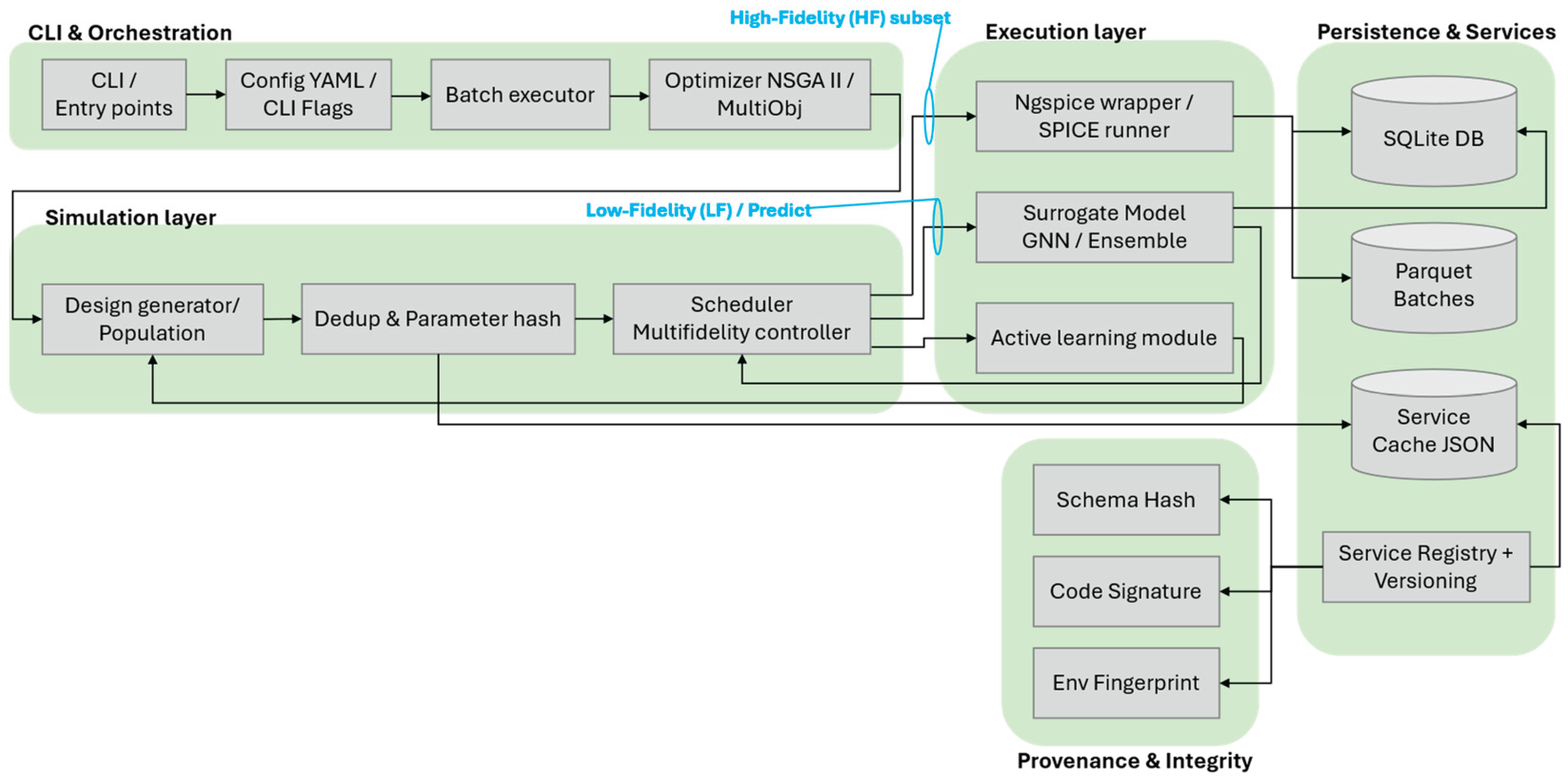
Figure 2.
Application lifecycle.
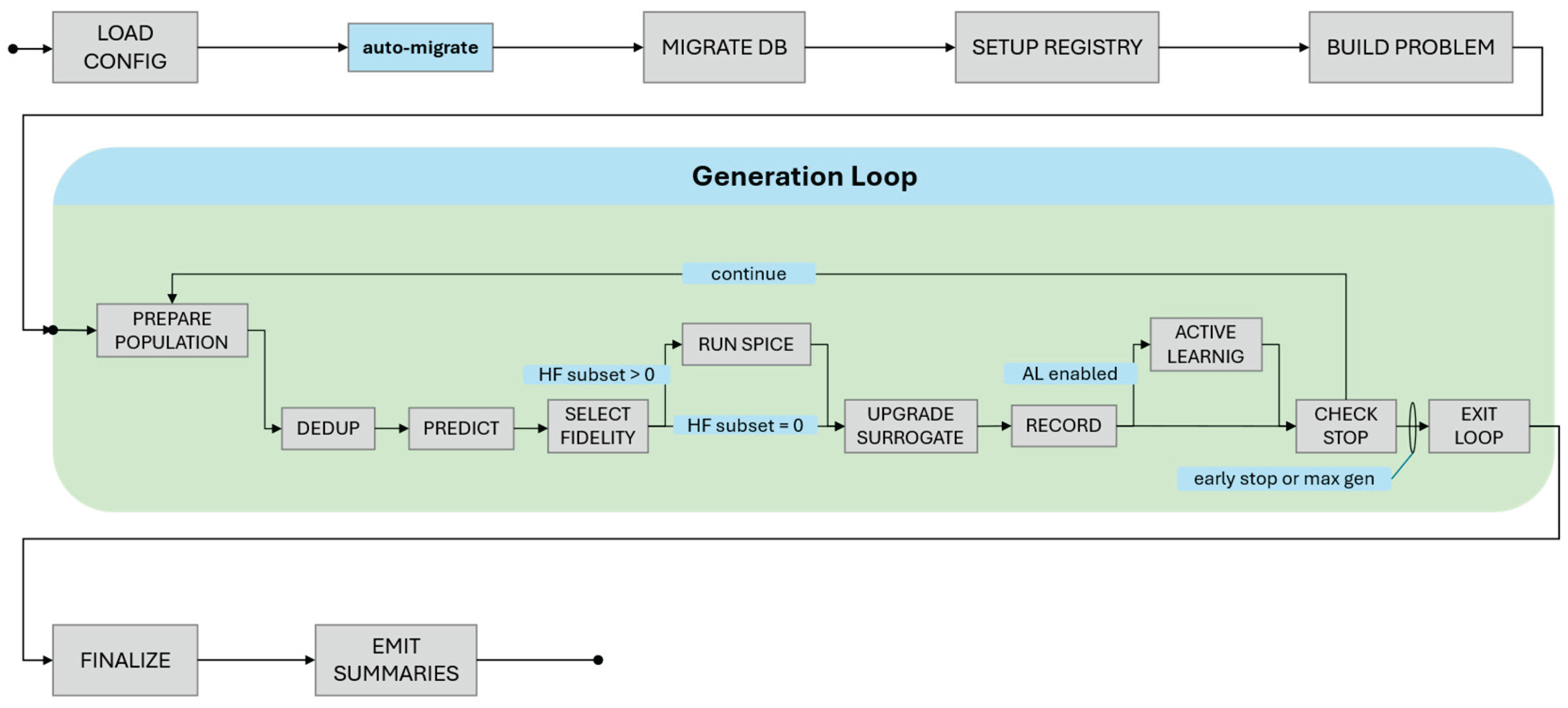
Figure 3.
Surrogate update and governance flow. A candidate model trained on new high-fidelity data is evaluated against the current best. If the error improves beyond a threshold, the model is checkpointed and the best metrics are updated; if performance degrades beyond tolerance, the system rolls back to the prior checkpoint. Penalty adaptation and surrogate update events are issued accordingly.
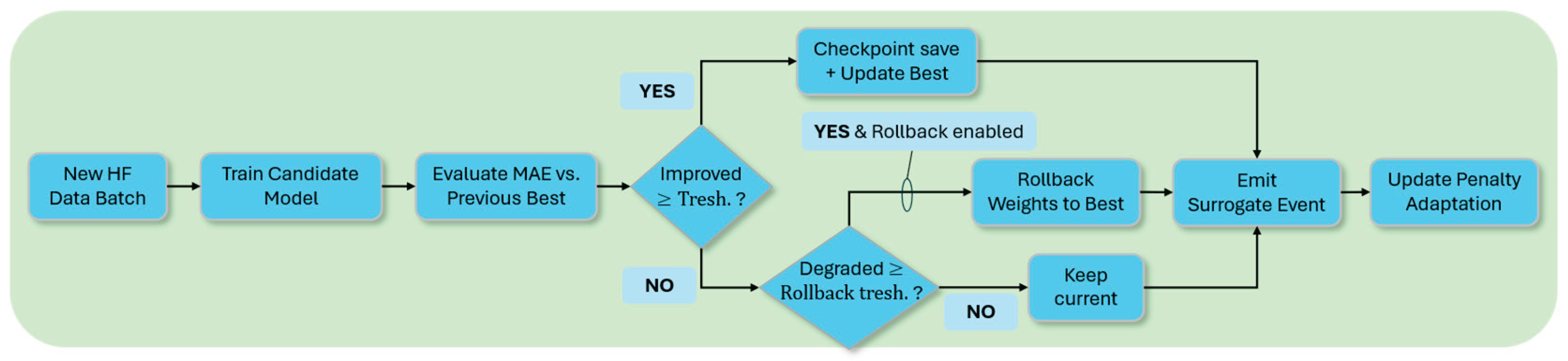
Figure 4.
Sequence diagram of main simulator modules interaction.
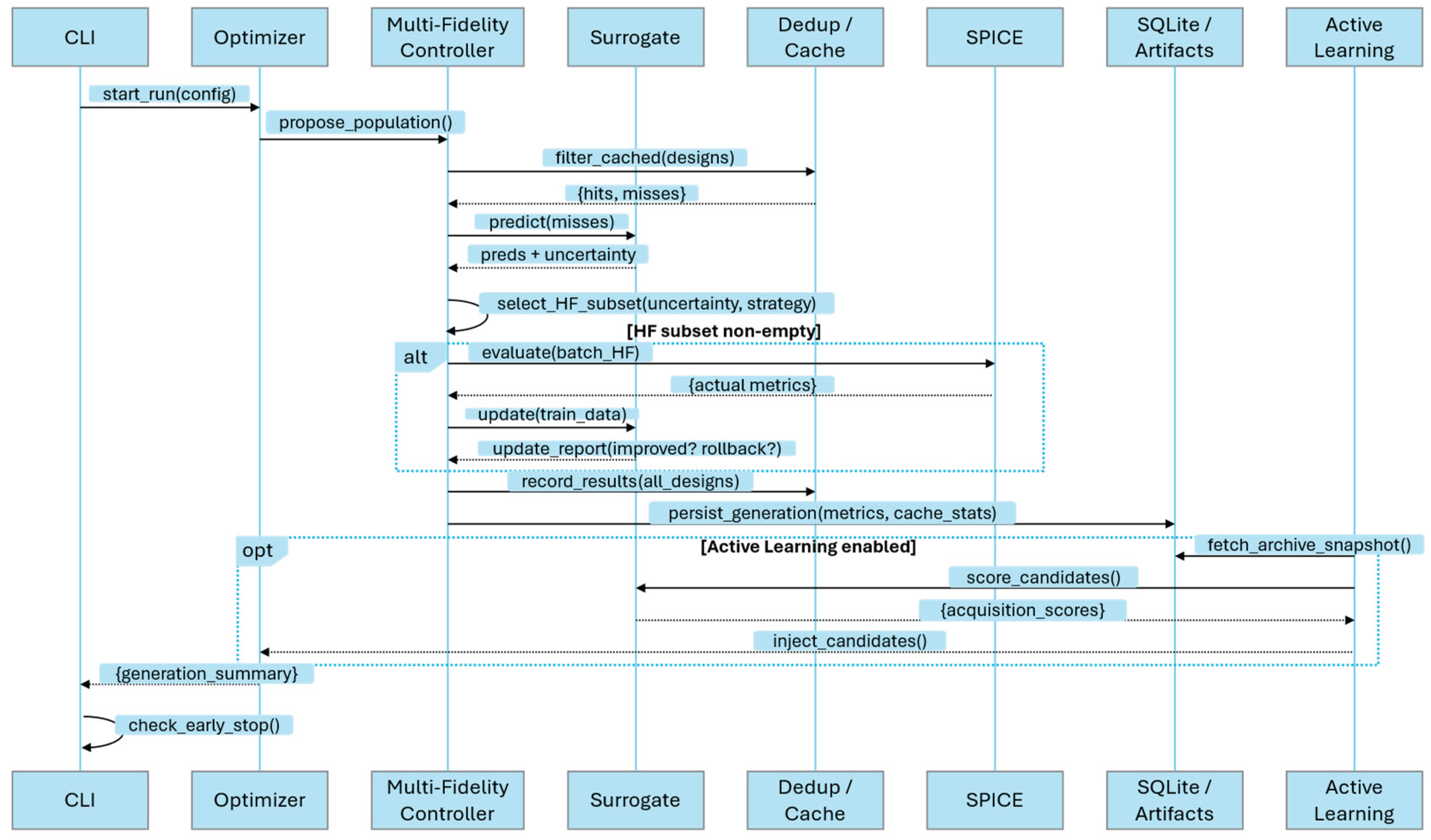
Figure 5.
Flow diagram of the cache subsystem. After parameter hashing, a cache hit directly reuses stored results, while a miss triggers evaluation and subsequent archival; eviction is applied when the design archive exceeds its capacity.
Figure 5.
Flow diagram of the cache subsystem. After parameter hashing, a cache hit directly reuses stored results, while a miss triggers evaluation and subsequent archival; eviction is applied when the design archive exceeds its capacity.
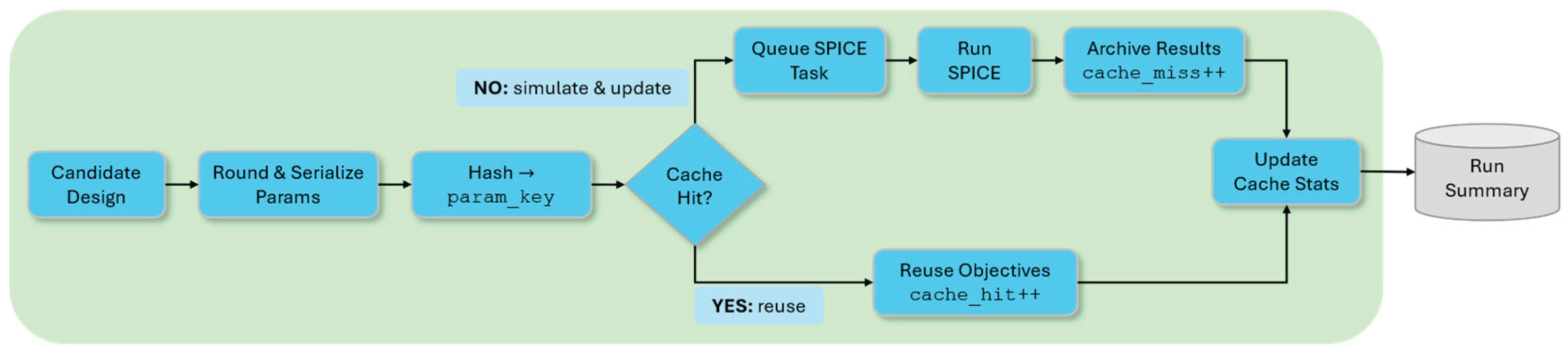
Figure 6.
Two-tier caching subsystem: a persistent design archive avoids redundant SPICE evaluations, while a lightweight service cache accelerates auxiliary tasks with provenance-aware invalidation. Both tiers provide metrics for monitoring efficiency and reuse trends.
Figure 6.
Two-tier caching subsystem: a persistent design archive avoids redundant SPICE evaluations, while a lightweight service cache accelerates auxiliary tasks with provenance-aware invalidation. Both tiers provide metrics for monitoring efficiency and reuse trends.
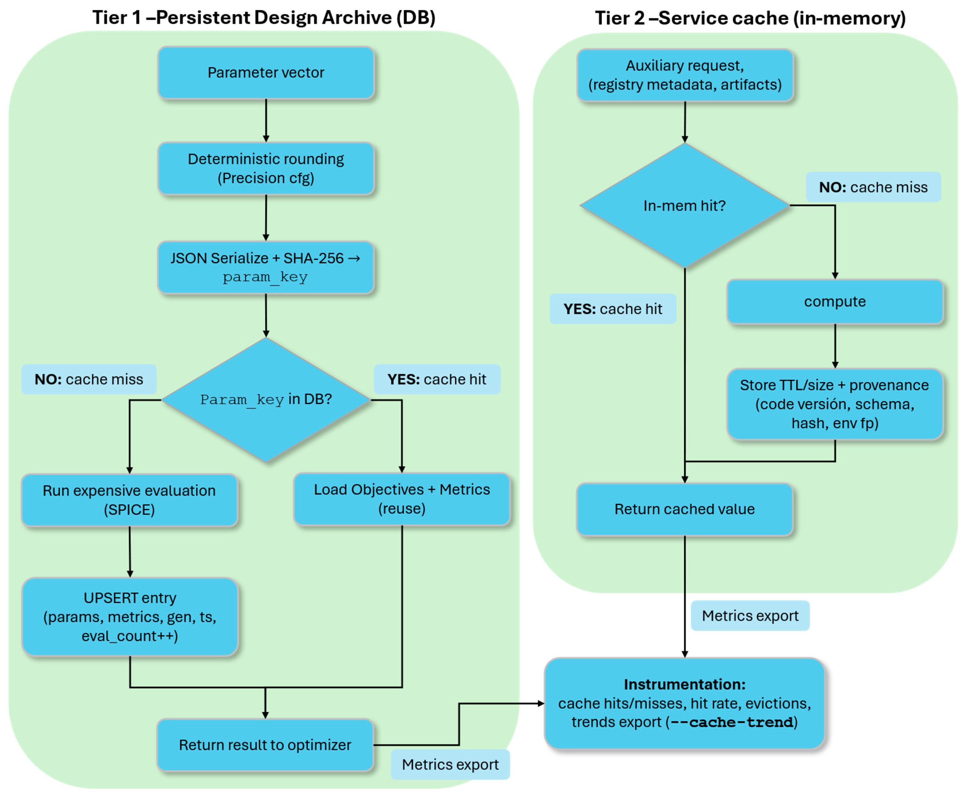
Figure 7.
Block diagram of the surrogate-assisted closed-loop optimization module of the simulator. Candidate solutions are generated by LHS/uniform sampling and scored via acquisition functions. Surrogate models (ensemble regressors or GNN) provide objective estimates and uncertainties. The evolutionary algorithm refines candidate populations, while the adaptive fidelity controller selects uncertain individuals for high-fidelity SPICE evaluation. Verified results update the dataset, retrain surrogates, and refresh the non-dominated archive until convergence is achieved.
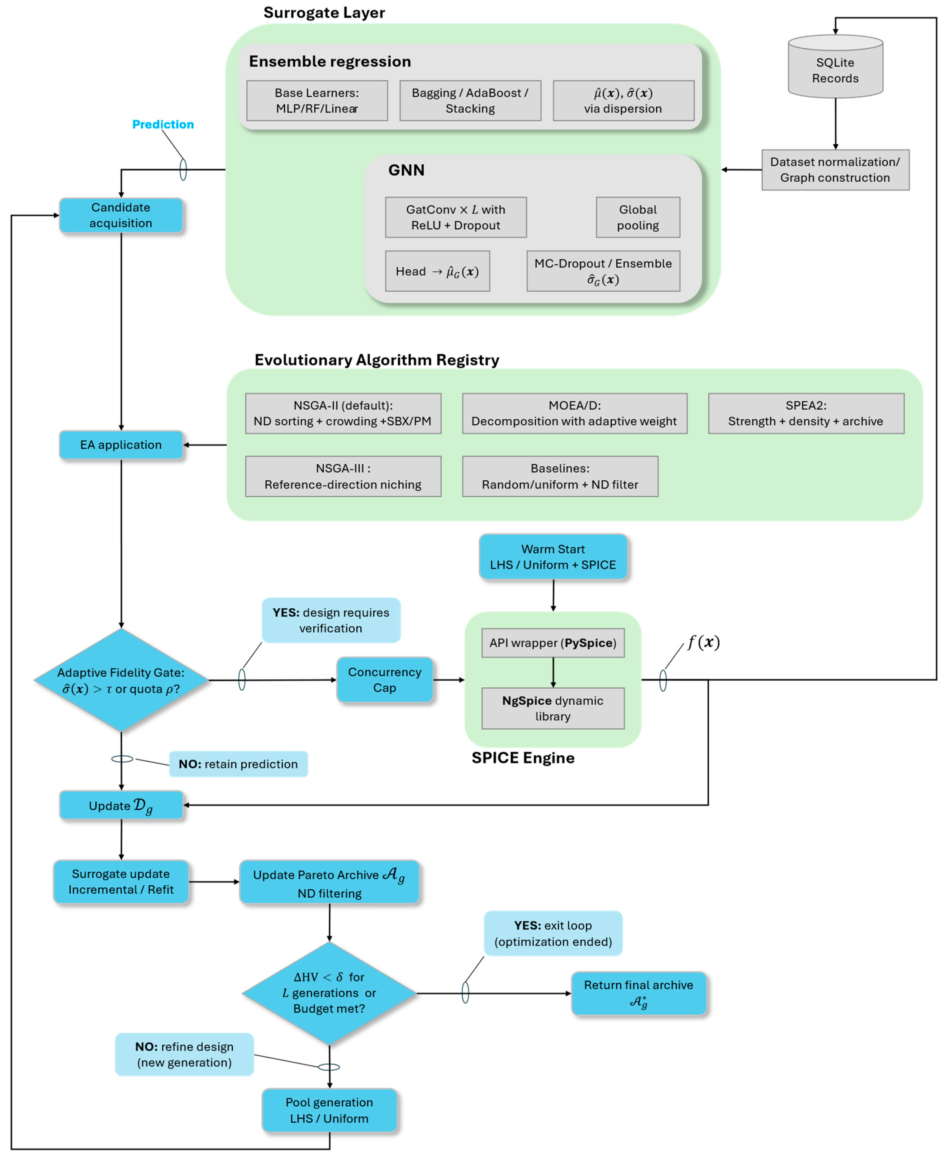
Figure 8.
CMOS operational amplifiers used for validation: (a) Folded-cascode op-amp (1 µm CMOS) with PMOS differential input pair and NMOS cascode mirror load; (b) Telescopic-cascode op-amp (1 µm CMOS); (c) Two-stage RC-compensated op-amp (50 nm CMOS) employing classical Miller compensation with a zero-nulling resistor for stability; (d) Two-stage transistor-compensated op-amp (50 nm CMOS) using indirect current feedback via a common-gate device.
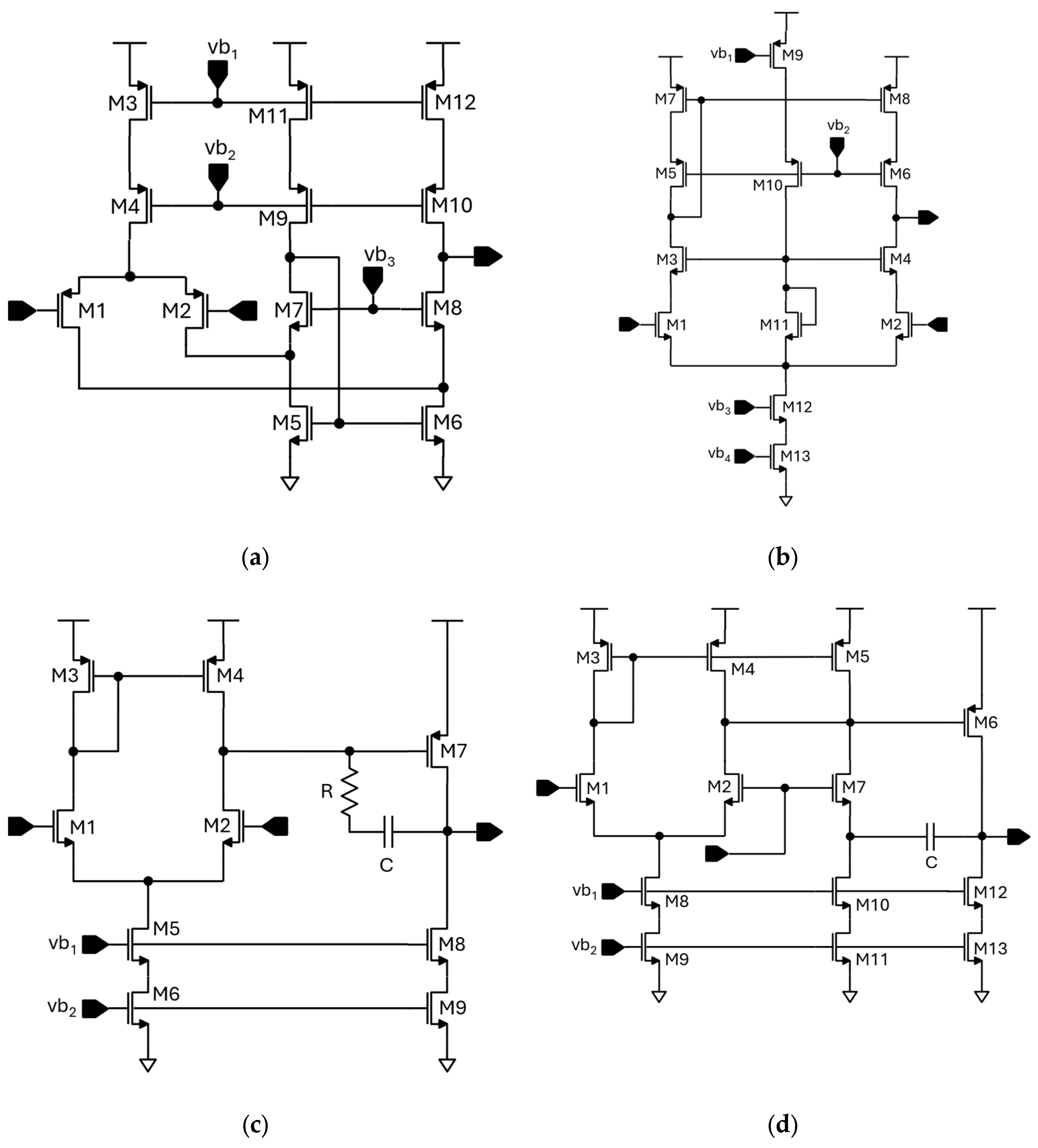
Figure 9.
Cache-hit rate and cumulative cache-hit rate evolution for SPICE-only optimization with NSGA-II, NSGA-III, and SPEA2, respectively, of the operational-amplifier topologies under test: (a-c) Miller-compensated differential amplifier; (d-f) Transistor-compensated differential amplifier; (g-i) folded-cascode op-amp; (l-n) Telescopic-cascode amplifier.
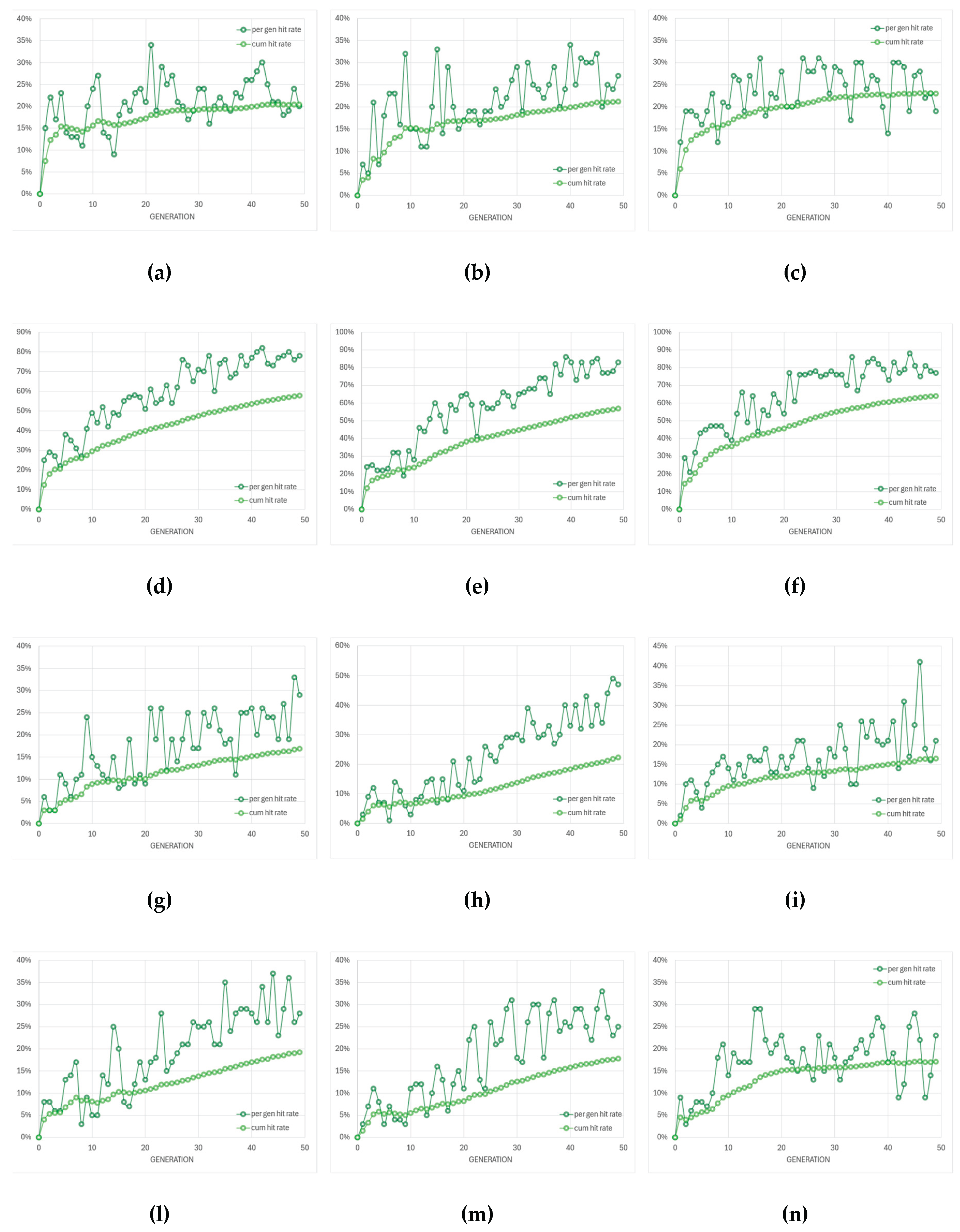
Figure 10.
Simulated vs. cached circuit evaluations per generation for a population of 100 individuals and for SPICE-only optimization with NSGA-II, NSGA-III, and SPEA2, respectively, of the operational-amplifier topologies under test: (a-c) Miller-compensated differential amplifier; (d-f) Transistor-compensated differential amplifier; (g-i) folded-cascode op-amp; (l-n) Telescopic-cascode amplifier.
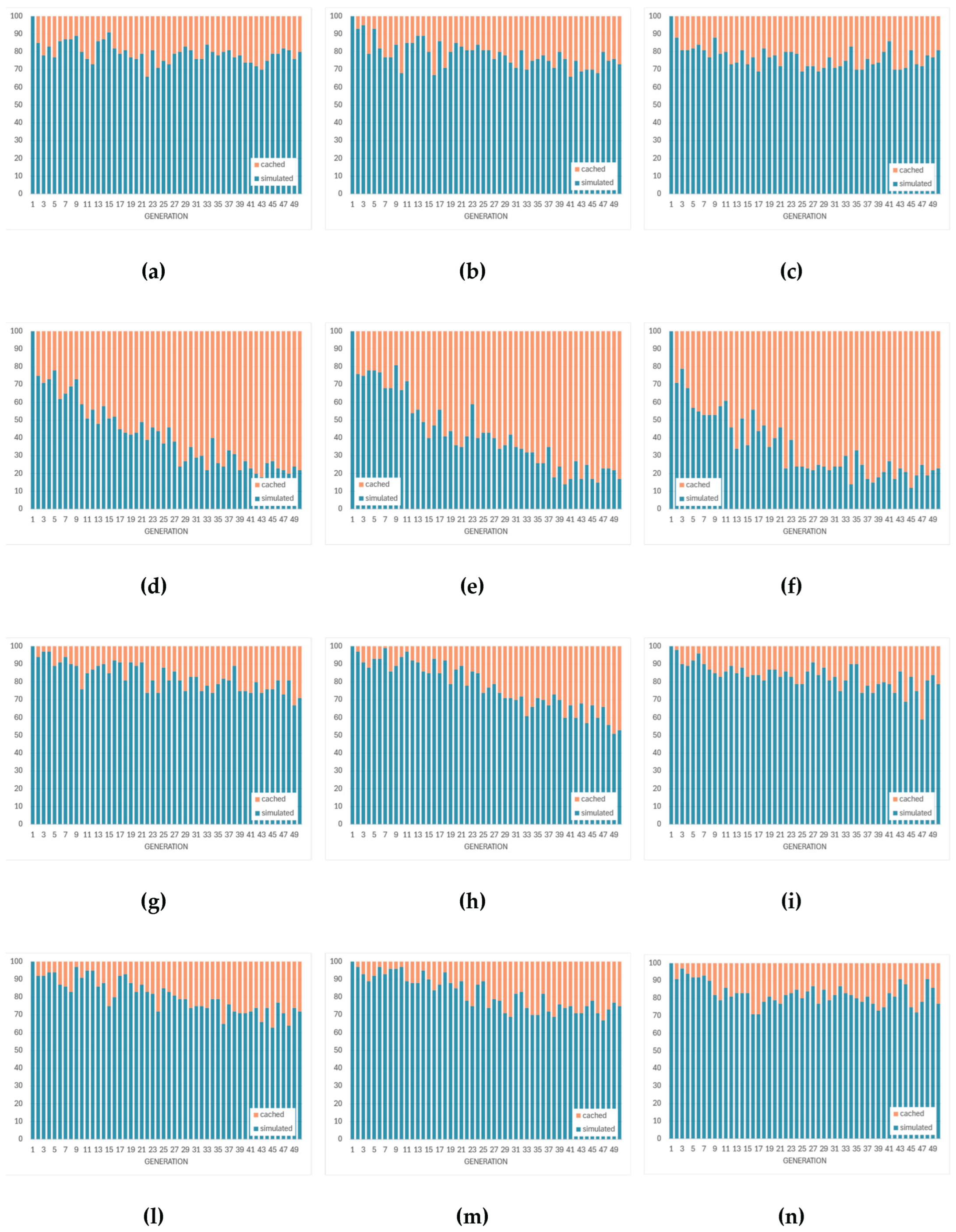
Figure 11.
Pareto-optimal solutions obtained from SPICE-only optimization for the operational-amplifier topologies under test using three evolutionary algorithms (NSGA-II, NSGA-III, and SPEA2, respectively). The explored design space is and : (a-c) Miller-compensated differential amplifier; (d-f) Transistor-compensated differential amplifier; (g-i) folded-cascode op-amp; (l-n) Telescopic-cascode amplifier.
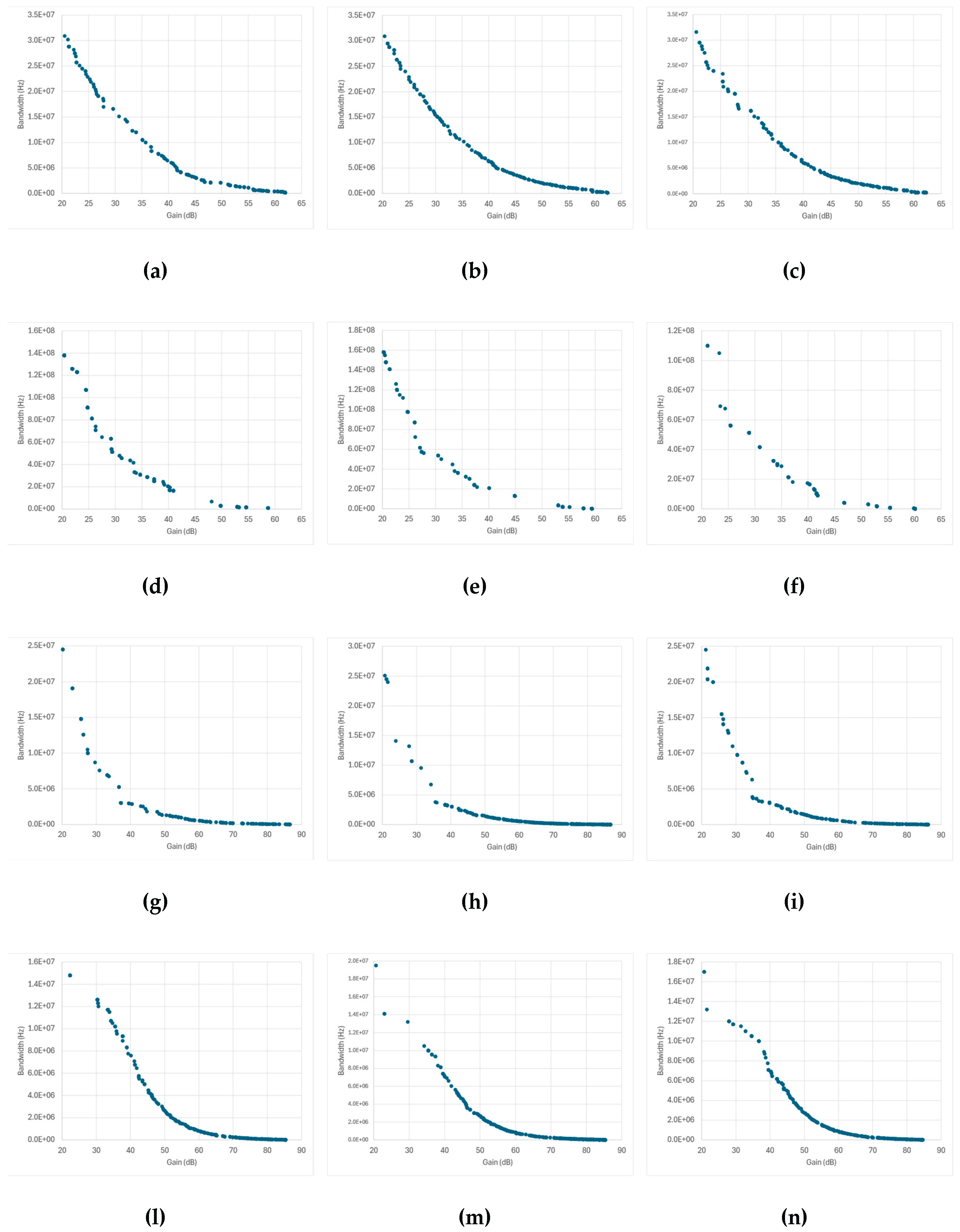
Figure 12.
Evolution of simulation throughput (SPICE simulations per second per generation) for different execution paradigms and SPICE-only optimization with NSGA-II, NSGA-III, and SPEA2, respectively, of the operational-amplifier topologies under test: (a-c) Miller-compensated differential amplifier; (d-f) Transistor-compensated differential amplifier; (g-i) folded-cascode op-amp; (l-n) Telescopic-cascode amplifier.
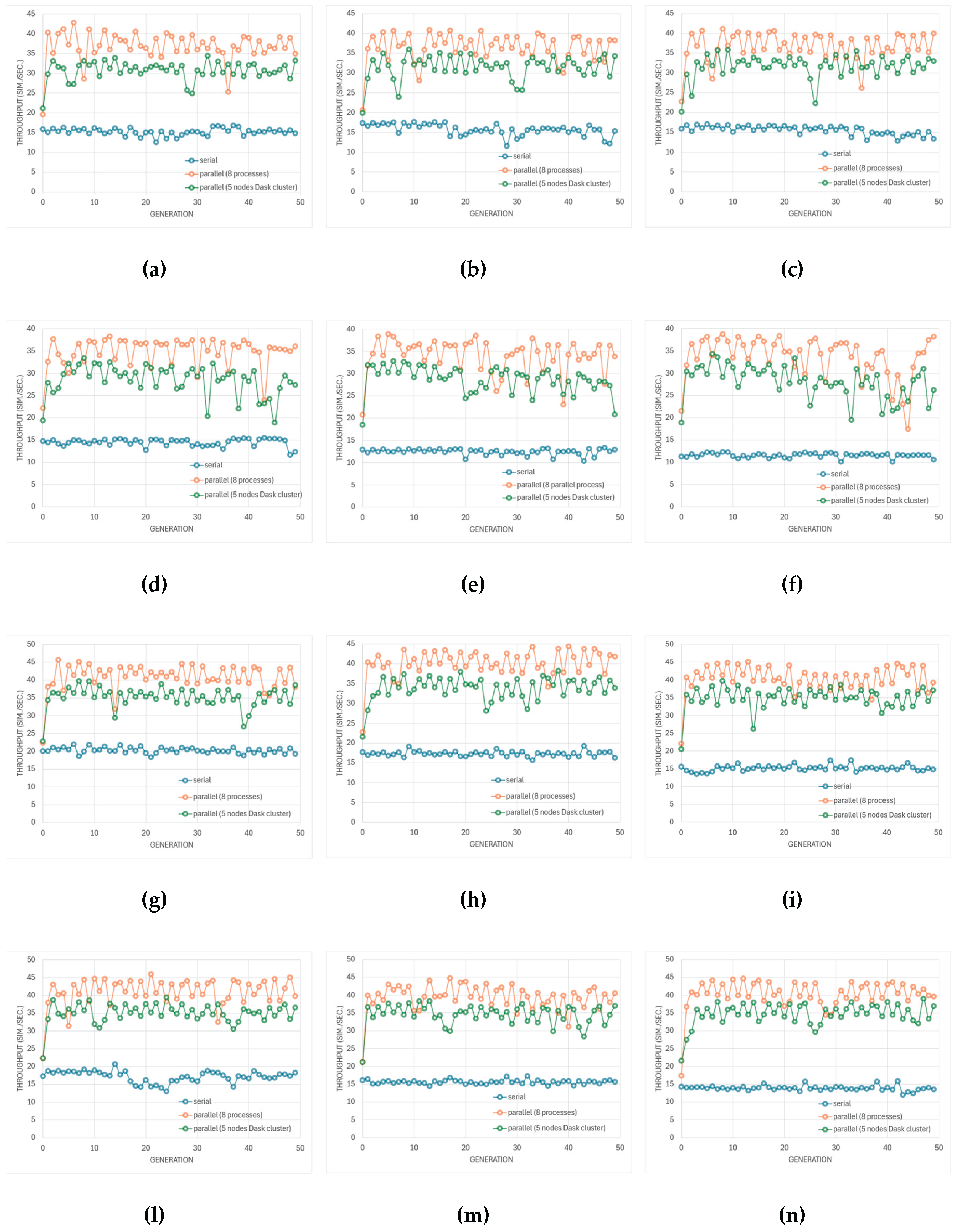
Figure 13.
Evolution of wall-clock time per generation for different execution paradigms and SPICE-only optimization with NSGA-II, NSGA-III, and SPEA2, respectively, of the operational-amplifier topologies under test: (a-c) Miller-compensated differential amplifier; (d-f) Transistor-compensated differential amplifier; (g-i) folded-cascode op-amp; (l-n) Telescopic-cascode amplifier.
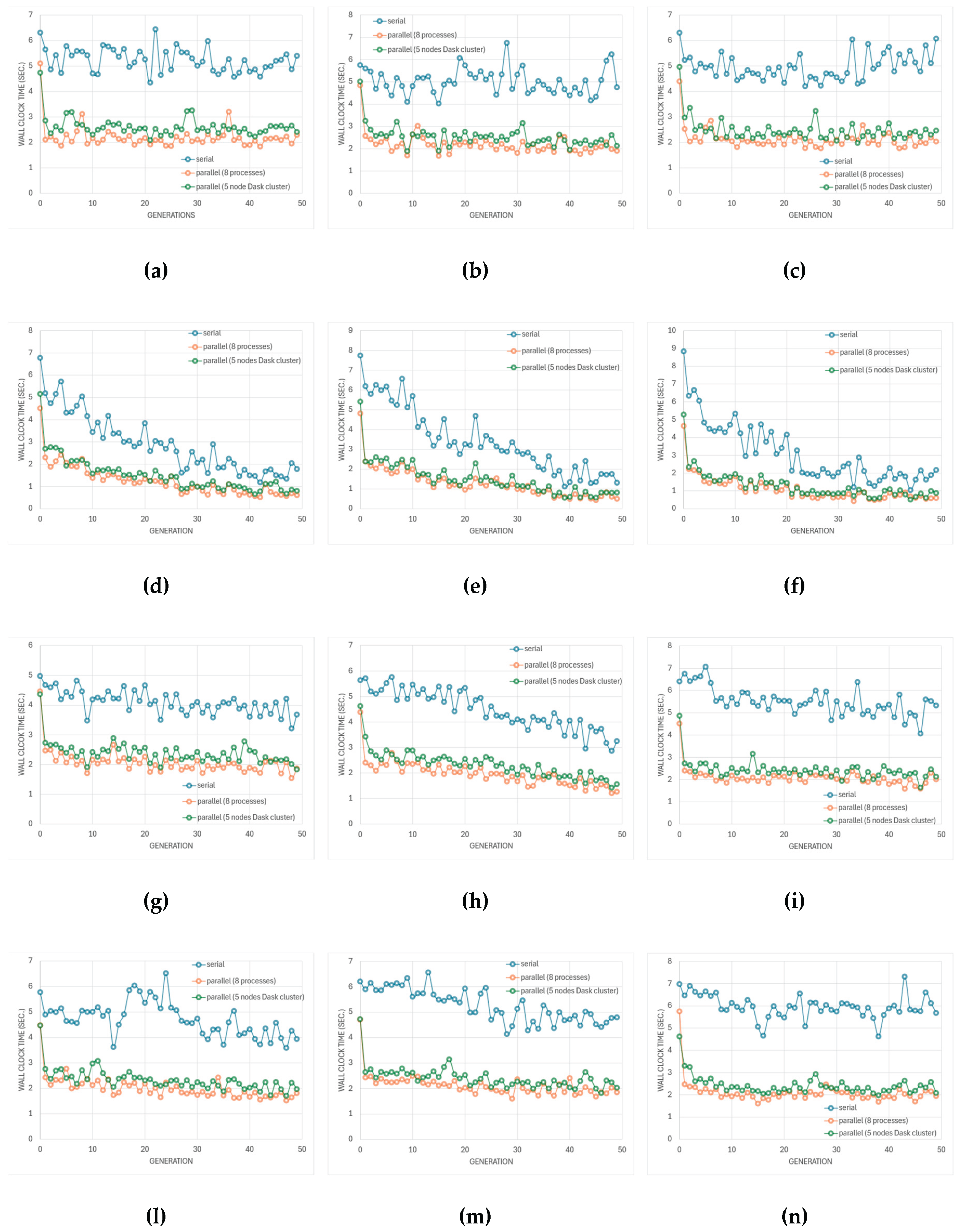
Figure 18.
Average wall-clock time per generation for the multi-fidelity optimization (MFO) runs across the tested amplifier topologies and multi-objective evolutionary algorithms (NSGA-II, NSGA-III, and SPEA2, respectively): (a-c) Miller-compensated differential amplifier; (d-f) Transistor-compensated differential amplifier; (g-i) folded-cascode op-amp; (l-n) Telescopic-cascode amplifier.
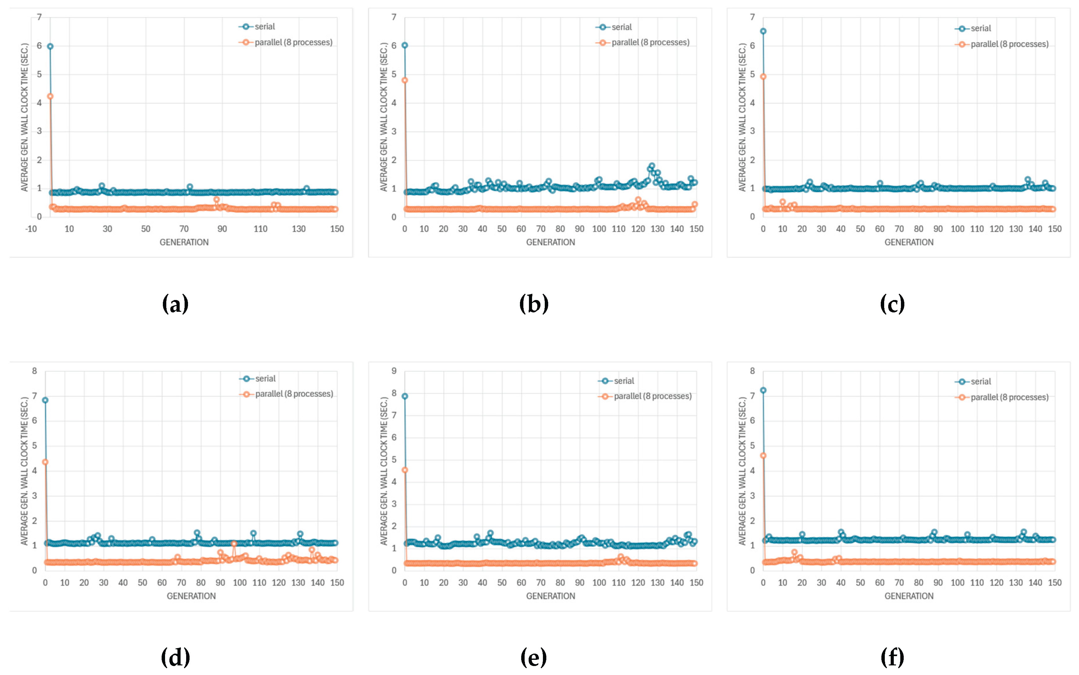
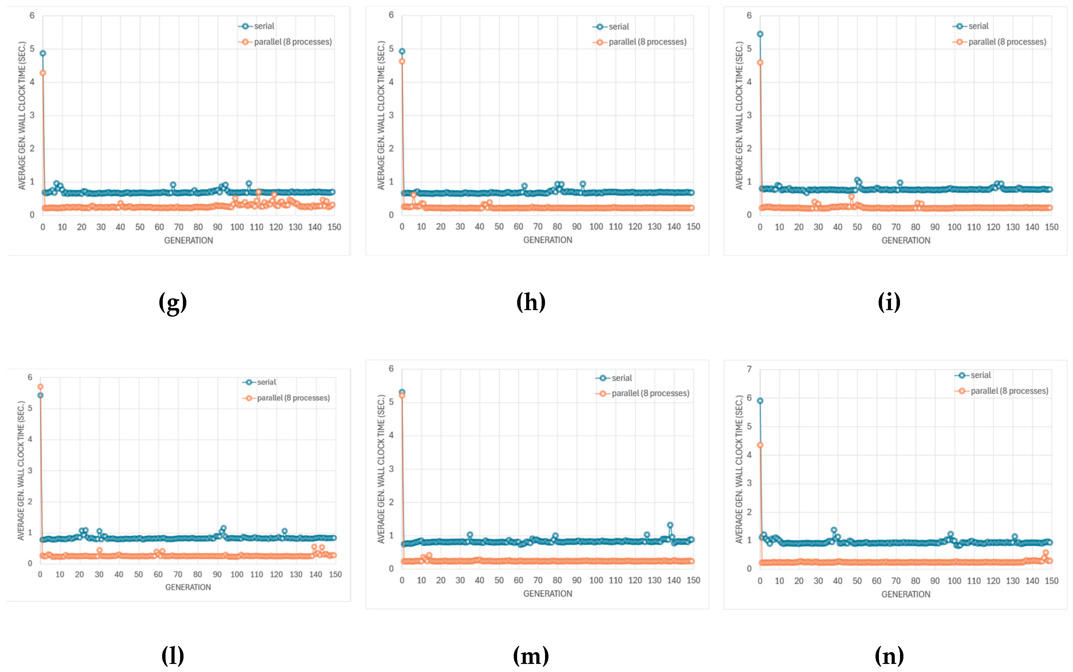

Table 1.
Sampling ranges for the designs under test (Figure 8).
Table 1.
Sampling ranges for the designs under test (Figure 8).
| Design | Device(s) | Sampling range |
|---|---|---|
| Folded cascode (1μm) | M1, M2, M5, M6, M9-M12 | W: 1-40μm, L: 1-3μm |
| M3, M4 | W: 1-80μm, L: 1-3μm | |
| M7, M8 | W: 1-20μm, L: 1-3μm | |
| Telescopic cascode (1μm) | M1-M4 | W: 1-20μm, L: 1-3μm |
| M5-M10, M12, M13 | W: 1-40μm, L: 1-3μm | |
| M11 | W: 1-20μm, L: 1-10μm | |
| RC-compensated op-amp (50nm) | M1-M9 | W: 0.1-1μm, L: 50-200nm |
| R | 1kΩ-100kΩ | |
| C | 0.1pF-0.5pF | |
| Transistor-compensated op-amp (50 nm) | M1, M2, M7, M10-M13 | W: 1-5μm, L: 50-200nm |
| M3-M6, M8, M9 | W: 1-10μm, L: 50-200nm | |
| C | 0.1pF-0.5pF |
Table 2.
Summary of simulation configuration.
| Parameter | Value/Setting | Description |
|---|---|---|
| Hardware | MacBook Pro (2.6 GHz Intel Core i7, 16 GB RAM) | Host system for all simulations |
| Objectives | Gain (20 – 100 dB), Bandwidth (1 kHz –1 GHz) | Primary optimization targets |
| Algorithms | NSGA-II / NSGA-III / SPEA2 / MOEA/D | Multi-objective evolutionary algorithms |
| Population / Generations | 200 / 150 (SGO & MF); 100 / 50 (SPICE-only) | GA configuration for main and baseline runs |
| Crossover / Mutation | 0.9 / 0.1 | Probabilities for genetic operators |
| Tournament Size | 2 | Number of competitors per selection round |
| Early Stopping | 0.01 (relative hypervolume change) | Convergence criterion |
| AC Analysis | 1 Hz – 1 GHz (100 points, 27 °C) | Frequency response for gain and bandwidth |
| Transient Analysis | 1 ns step, 2 µs duration | Slew-rate evaluation |
| SPICE Tolerances | reltol = 1e-3, abstol = 1e-12, vntol = 1e-6 | Numerical solver settings |
| Parallelism | Enabled (processes or local Dask cluster) | Concurrent circuit evaluations |
| Cache Precision | 6 decimal places | Design deduplication threshold |
| DoE Sampling | 100 Monte Carlo samples | Training data for surrogate and MF models |
| Parameter Ranges | See Table 1 | Monte Carlo design space |
| Correlation | ρ ∈ [0.1, 0.2] | Weak positive correlation |
| Random Seed | Fixed (across all runs) and set to 101 | Ensures fair cross-algorithm comparison |
Table 3.
Summary of average simulation throughput and average wall-clock time per generation for all amplifier topologies and execution modes. Results are reported for sequential execution, process-based parallelism (8 concurrent SPICE processes), and a 5-node local Dask cluster. The speedup columns quantify the ratio of sequential to parallel wall-clock time for each configuration.
| Design | Algorithm |
Average throughput per simulation mode [sim/s] |
Average wall-clock time per simulation mode [s] |
Speedup (processes) | Speedup (Dask) |
| Miller-compensated op-amp | NSGA-II | 15.22 / 36.76 / 30.69 | 5.24 / 2.21 / 2.62 | 2.37 | 2.00 |
| NSGA-III | 15.74 / 36.48 / 31.50 | 5.03 / 2.20 / 2.54 | 2.29 | 1.98 | |
| SPEA2 | 15.54 / 36.69 / 31.65 | 4.98 / 2.13/ 2.47 | 2.34 | 2.02 | |
| Transistor-compensated op-amp | NSGA-II | 14.48 / 34.78 / 28.48 | 2.91 / 1.25 / 1.49 | 2.33 | 1.95 |
| NSGA-III | 12.47 / 33.95 / 28.78 | 3.44 / 1.29 / 1.51 | 2.67 | 2.28 | |
| SPEA2 | 11.58 / 33.71 / 28.13 | 3.11 / 1.08 / 1.28 | 2.88 | 2.43 | |
| Folded cascode amplifier | NSGA-II | 20.27 / 40.78 / 35.20 | 4.10 / 2.07 / 2.38 | 1.98 | 1.72 |
| NSGA-III | 17.33 / 40.09 / 33.90 | 4.49/ 1.97 / 2.32 | 2.28 | 1.94 | |
| SPEA2 | 15.17 / 40.43 / 34.96 | 5.53 / 2.10 / 2.42 | 2.63 | 2.28 | |
| Telescopic cascode amplifier | NSGA-II | 17.22 / 40.95 / 35.08 | 4.73 / 2.01 / 2.33 | 2.35 | 2.03 |
| NSGA-III | 15.62 / 39.33 / 34.48 | 5.27 / 2.12 / 2.41 | 2.49 | 2.19 | |
| SPEA2 | 13.91 / 40.31 / 34.75 | 5.97 / 2.11 / 2.42 | 2.83 | 2.47 |
Table 4.
Summary of MOEA/D optimization statistics for the four amplifier topologies. Each run processed 5000 total individuals using sequential execution with identical solver and stopping parameters.
Table 4.
Summary of MOEA/D optimization statistics for the four amplifier topologies. Each run processed 5000 total individuals using sequential execution with identical solver and stopping parameters.
| Design | Wall clock Time [s] |
Total individuals |
Total simulated |
Total cached |
Cache hit rate |
Throughput [sim/sec] |
|---|---|---|---|---|---|---|
| Miller-compensated op-amp | 110.96 | 5000 | 1438 | 3562 | 0.712 | 12.96 |
| Transistor-compensated op-amp | 67.34 | 5000 | 437 | 4563 | 0.913 | 6.49 |
| Folded cascode amplifier |
133.92 | 5000 | 1396 | 3604 | 0.721 | 10.42 |
| Telescopic cascode amplifier |
132.43 | 5000 | 1307 | 3693 | 0.739 | 9.97 |
Table 5.
Summary of MOEA/D optimization statistics with PyMoo parallelization for the four amplifier topologies. Each run processed 5000 total individuals with identical solver and stopping parameters.
Table 5.
Summary of MOEA/D optimization statistics with PyMoo parallelization for the four amplifier topologies. Each run processed 5000 total individuals with identical solver and stopping parameters.
| Design | Wall clock Time [s] |
Total individuals |
Total simulated |
Total cached |
Cache hit rate |
Throughput [sim/sec] |
|---|---|---|---|---|---|---|
| Miller-compensated op-amp | 120.31 | 5000 | 1583 | 3417 | 0.683 | 13.16 |
| Transistor-compensated op-amp | 59.40 | 5000 | 339 | 4661 | 0.932 | 5.71 |
| Folded cascode amplifier |
133.35 | 5000 | 1376 | 3624 | 0.725 | 10.32 |
| Telescopic cascode amplifier |
122.08 | 5000 | 1165 | 3835 | 0.767 | 9.54 |
Table 6.
Summary of MAE statistics for the surrogate model across 12 independent surrogate-guided optimization runs per amplifier topology. Each entry reports the range (minimum–maximum) and median of the initial, final, and best MAE values computed on the validation batches.
Table 6.
Summary of MAE statistics for the surrogate model across 12 independent surrogate-guided optimization runs per amplifier topology. Each entry reports the range (minimum–maximum) and median of the initial, final, and best MAE values computed on the validation batches.
| Design | Initial MAE (min–max, median) |
Final MAE (min–max, median) |
Best MAE (min–max, median) |
Mean Improvement [%] |
|---|---|---|---|---|
| Miller-compensated op-amp | 0.3780–0.5197 (median 0.4146) | 0.2061–0.3550 (median 0.2217) | 0.0543–0.3550 (median 0.1276) | 35.3% |
| Transistor-compensated op-amp | 0.0957–0.1204 (median 0.1052) | 0.0163–0.1234 (median 0.0756) | 0.0019–0.0767 (median 0.0590) | 42.8% |
| Folded cascode amplifier |
0.0277–0.1121 (median 0.0312) | 0.0059–0.0371 (median 0.0222) | 0.0017–0.0312 (median 0.0222) | 43.5% |
| Telescopic cascode amplifier |
0.3091–0.3372 (median 0.3299) | 0.0839–0.2463 (median 0.2155) | 0.0159–0.2155 (median 0.1825) | 44.1% |
Table 7.
Summary of MAE statistics across 12 independent multi-fidelity optimization runs per amplifier topology. Each entry reports the range (minimum–maximum) and median of the initial, final, and best MAE values computed on the validation batches together with the average relative improvement.
Table 7.
Summary of MAE statistics across 12 independent multi-fidelity optimization runs per amplifier topology. Each entry reports the range (minimum–maximum) and median of the initial, final, and best MAE values computed on the validation batches together with the average relative improvement.
| Design | Initial MAE (min–max, median) |
Final MAE (min–max, median) |
Best MAE (min–max, median) |
Mean Improvement [%] |
|---|---|---|---|---|
| Miller-compensated op-amp | 0.3780–0.5197 (median 0.4146) | 0.2061–0.3550 (median 0.2217) | 0.0543–0.3550 (median 0.1276) | 63.6% |
| Transistor-compensated op-amp | 0.0957–0.1204 (median 0.1052) | 0.0163–0.1234 (median 0.0756) | 0.0019–0.0767 (median 0.0590) | 41.4% |
| Folded cascode amplifier |
0.0277–0.1121 (median 0.0312) | 0.0059–0.0371 (median 0.0222) | 0.0017–0.0312 (median 0.0222) | 63.6% |
| Telescopic cascode amplifier |
0.3091–0.3372 (median 0.3299) | 0.0839–0.2463 (median 0.2155) | 0.0159–0.2155 (median 0.1825) | 41.4% |
Table 8.
Average wall-clock time per generation and parallel execution efficiency for multi-fidelity optimization (MFO). Each configuration was executed under identical solver and adaptive-fidelity settings. Mean and total wall-clock times are reported for both serial and parallel execution (8 workers). Parallel performance metrics include wall-clock speedup, parallel efficiency (relative to 8 ideal workers)
| Design | Algorithm | Mean Wall-Clock Time [s/gen] | Total Wall-Clock [s] | Wall-Clock Speedup | Parallel Efficiency [%] | Time Reduction [%] | Per-Generation Speedup |
|---|---|---|---|---|---|---|---|
| Differential op-amp | NSGA-II | 0.91 → 0.32 | 151.4 → 65.3 | 2.32× | 29.0 | 56.9 | 2.83× |
| NSGA-III | 1.10 → 0.33 | 188.8 → 67.9 | 2.78× | 34.8 | 64.1 | 3.37× | |
| SPEA2 | 1.06 → 0.32 | 180.2 → 72.1 | 2.50× | 31.3 | 60.0 | 3.25× | |
| Transistor-compensate op-amp | NSGA-II | 1.17 → 0.43 | 188.8 → 78.0 | 2.42× | 30.3 | 58.7 | 2.71× |
| NSGA-III | 1.29 → 0.39 | 209.7 → 71.0 | 2.95× | 36.9 | 66.1 | 3.33× | |
| SPEA2 | 1.30 → 0.41 | 213.2 → 77.1 | 2.77× | 34.6 | 63.8 | 3.17× | |
| Folded cascode | NSGA-II | 0.73 → 0.31 | 121.6 → 59.6 | 2.04× | 25.5 | 51.0 | 2.36× |
| NSGA-III | 0.72 → 0.26 | 121.7 → 52.3 | 2.33× | 29.1 | 57.1 | 2.71× | |
| SPEA2 | 0.82 → 0.27 | 143.1 → 59.7 | 2.40× | 30.0 | 58.3 | 3.06× | |
| Telescopic cascode | NSGA-II | 0.87 → 0.30 | 144.4 → 54.7 | 2.64× | 33.0 | 62.2 | 3.14× |
| NSGA-III | 0.86 → 0.27 | 166.6 → 58.2 | 2.86× | 35.8 | 65.1 | 3.49× | |
| SPEA2 | 0.98 → 0.28 | 188.8 → 78.0 | 2.42× | 30.3 | 58.7 | 2.71× |
Table 9.
Comparative summary of the three optimization modes examined in this work.
| Feature | SPICE-Only | Surrogate-Guided Optimization (SGO) | Multi-fidelity Optimization (MFO) |
|---|---|---|---|
| . Evaluation method | Pure SPICE | Hybrid (surrogate + periodic SPICE) | Adaptive hybrid (uncertainty-driven SPICE fraction) |
| Speedup | Baseline (1×) | ≈ 20× (≈ 95% reduction) | ≈ 10× (≈ 90% reduction) |
| Accuracy guarantee | Perfect (All SPICE) | Approximate (final sweep verifies) | Near-perfect (adaptive verification ensures quality) |
| Computational cost | High | Low-Medium | Medium |
| Model training | None | Online (continuous) | Online with rollback |
| Uncertainty quantification | Not applicable | Yes (MC-dropout/ensemble) | Yes (with adaptive penalty) |
| Best suited for | Small design problems | Large design spaces/expensive simulations | Accuracy-critical applications |
| 1 | Optuna is a general-purpose, define-by-run hyperparameter optimization framework. |
| 2 | In the context of the closed-loop optimization loop the archive is simply the set of non-dominated solutions (the current approximation of the Pareto front) that the simulator has collected so far. Formally, at generation we maintain: |
Disclaimer/Publisher’s Note: The statements, opinions and data contained in all publications are solely those of the individual author(s) and contributor(s) and not of MDPI and/or the editor(s). MDPI and/or the editor(s) disclaim responsibility for any injury to people or property resulting from any ideas, methods, instructions or products referred to in the content. |
© 2025 by the authors. Licensee MDPI, Basel, Switzerland. This article is an open access article distributed under the terms and conditions of the Creative Commons Attribution (CC BY) license (http://creativecommons.org/licenses/by/4.0/).
Copyright: This open access article is published under a Creative Commons CC BY 4.0 license, which permit the free download, distribution, and reuse, provided that the author and preprint are cited in any reuse.


