Submitted:
05 November 2025
Posted:
07 November 2025
You are already at the latest version
Abstract
Canonical market microstructure theories, validated in liquid financial markets, are often misapplied to illiquid power futures. This study introduces the Impact-Inventory Parity (IIP) parameter Ψ, bridging the Kyle (information-based) and Ho-Stoll (inventory-based) models, and uses agent-based simulations to test its validity in thin markets. We uncover a critical asymmetry: while competition consistently pushes markets towards inventory dominance, the countervailing effect of non-linear inventory costs systematically weakens as markets thin due to lower inventory variance. This creates a structural bias toward inventory dominance Ψ=1 that persists despite strong convex penalties. Adaptive behaviour revealed a stability paradox, causing severe parity breakdown that was amplified by liquidity, not thinness. Parameter space analysis showed market stability rests equally on three structural pillars: participation, liquidity, and information quality. Among stable markets, information quality dominates regime outcomes, while adaptative behaviour acts as a critical threshold where small changes can trigger immediate market collapse. Across the physically plausible parameter space, inventory-dominated regimes comprise the vast majority (73%) of configurations, while the balanced-risk conditions predicted by classical theory are rare (8%), confirming parity as a narrow, fragile equilibrium. The framework proves robust in thin, fragmented markets—precisely where canonical models fail, while becoming unreliable in the liquid, centralized venues where those models were validated.
Keywords:
market microstructure
; power futures markets
; market maker
; agent-based modeling
; liquidity provision
; Kyle model
; inventory risk
; thin markets
; electricity trading
1. Introduction
1.1. The Liquidity Challenge in Power Futures Markets
Power futures markets often exhibit low liquidity. Despite billions in annual trading volumes— concentrated primarily in near-term contracts —bid-ask spreads in electricity futures often exceed comparable financial markets by an order of magnitude [1,2]. This illiquidity imposes severe economic costs precisely when these markets are most needed. The global energy transition depends on efficient price discovery and risk management tools for renewable energy investments [3]. Yet the very markets designed to provide these functions can suffer from chronic illiquidity, particularly for contracts extending beyond one year.
The consequences cascade throughout the energy system. Wide spreads increase transaction costs for hedging. Volatile prices complicate investment planning [4]. Limited market depth restricts large participants from managing portfolio risks effectively. Most critically, inadequate liquidity creates barriers to capital formation for clean energy infrastructure. Renewable developers struggle to secure long-term revenue certainty, while utilities cannot efficiently hedge variable generation exposure [5,6]. Industrial consumers face elevated costs for managing price risk.
Market makers represent the standard financial solution to these liquidity challenges. By continuously quoting two-sided markets and absorbing temporary order imbalances, they typically reduce spreads, increase volumes, and improve price efficiency. Recognizing this potential, regulators worldwide are actively developing market maker programs for power futures markets [7]. The Agency for the Cooperation of Energy Regulators (ACER), national authorities across Europe, and the U.S. Commodity Futures Trading Commission are all exploring mechanisms to enhance liquidity. However, these initiatives often import program designs and theoretical frameworks directly from liquid financial markets. This paper addresses this gap by analyzing the effectiveness of standard market maker models in an environment characterized not by information asymmetry, but by structural illiquidity and inventory risk. We ask: under what conditions can market maker programs succeed when their foundational assumptions of competitive pressure and deep order flow are absent?
1.2. Canonical Models of Market Making
The Kyle [8] model provides the foundational framework for analyzing market maker effectiveness under information asymmetry. This cornerstone of market microstructure theory elegantly captures how adverse selection affects liquidity provision. Crucially, the model assumes market makers are perfectly competitive (or operate under a market-clearing mandate), leading to a zero-expected-profit condition in steady state. This zero-profit assumption, however, is unlikely to hold in illiquid markets where the lack of competition allows market makers to wield significant pricing power. The focus is squarely on how they process private information signals embedded in order flow. The model derives closed-form solutions for optimal market maker pricing when facing potentially informed traders. Kyle’s lambda parameter precisely quantifies market depth as the price impact per unit of order flow.
Kyle’s theoretical predictions have received extensive empirical validation across liquid, anonymous financial markets. Studies confirm the predicted relationships between order flow and price changes [9]. Research documents the inverse correlation between informed trading intensity and market depth. The model’s insights about spread determinants and volume patterns consistently match observed market behaviour. This empirical success has established Kyle’s framework as the standard benchmark for analyzing liquidity provision and market maker programs [10,11]. This empirical success, however, is confined to the very markets that power futures are not: deep, anonymous, and information-rich. The structural features of energy markets call the direct applicability of these findings into question.
Analytical work in market microstructure has also explored other drivers of liquidity provision. The model of Ho and Stoll [12] represents a foundational framework focusing on inventory risk as a primary driver of market maker behaviour (see also Amihud and Mendelson [13]). In contrast to the Kyle framework, Ho-Stoll features a market maker acting as a risk manager rather than an information processor; quotes are influenced by the need to manage an unbalanced portfolio. A market maker holding excess inventory will lower its quotes to attract buyers and deter sellers, and vice versa. This introduces a distinct motivation for quoting behaviour and provides a richer, though still highly stylized, model of liquidity provision. Together, the Kyle and Ho-Stoll models represent the canonical benchmarks for information-based and inventory-based market making, respectively.
Beyond these two canonical models, our analysis also draws on related streams of market microstructure theory. The framework of Glosten and Milgrom [14] refines the modeling of adverse selection in sequential trade, while research by Easley and O’Hara [15] highlights the information content revealed by trade size, a critical factor in thin markets. More directly, recent work by Pena and Rodríguez [16] provides the first empirical examination of market maker programs in European electricity futures. Our paper builds on this by providing a theoretical foundation for their findings and exploring the strategic behaviour of market makers, a topic previously analyzed in other thin commodity markets by Antón and Bushnell [17] and Kumar and Seppi [18].
1.3. The Mismatch Between Theory and Power Market Reality
Power markets violate the assumptions of these canonical models in fundamental ways. These disconnects span two critical dimensions—– physical characteristics and market structure –—that challenge the frameworks’ applicability, particularly in thin markets, defined here as markets with a finite number of buyers and sellers.
First, electricity’s physical characteristics differ radically from financial assets [19,20]. Unlike storable commodities, electricity cannot be easily inventoried, which profoundly shapes hedging needs and prevents market makers from managing positions through a physical spot market. The grid itself imposes structural constraints: transmission bottlenecks fragment the market into location-specific prices, while generation faces hard capacity and ramping limits that restrict supply elasticity [21]. The trading structure also departs from financial archetypes; while futures trade continuously, their pricing is inextricably linked to discrete, high-volume daily auctions in the underlying physical market, creating a distinct informational heartbeat.
Second, the behavioural and informational assumptions of canonical models fail. The assumption of anonymity is frequently violated; participants are registered entities with known generation or load obligations, allowing for reputation-based behaviours that are absent from anonymous markets. Instead of a single informed trader facing a sea of uninformed noise traders, the market consists of strategic, oligopolistic generators with known market power [22,23] and load-serving entities with highly predictable hedging needs. Crucially, information often arrives through public channels, such as weather forecasts or grid condition reports, rather than the private signals central to Kyle’s framework. This public information structure and non-anonymous, strategic environment fundamentally alters the nature of liquidity provision.
The systematic violation of these assumptions renders traditional equilibrium analysis inadequate for power markets. In thin markets, participants recognize their impact on prices and adapt their behaviour accordingly, moving away from the price-taking behaviour assumed in competitive equilibrium models. Analytical models achieve tractability only by eliminating these defining features: strategic interaction, non-storability, and imperfect competition. Relaxing these assumptions simultaneously destroys closed-form solutions.
1.4. The Role of Agent-Based Modeling
Agent-based models (ABMs) offer a promising methodological approach to address these analytical challenges [24,25]. ABMs allow heterogeneous agents to embody distinct operational characteristics, information sets, and realistic behavioural rules, including adaptive heuristics and strategic behaviours that are difficult to model analytically. While this departs from the strict assumption of idealized payoff maximization used in equilibrium analysis, it allows us to model the complex interactions and emergent market dynamics characteristic of real-world power trading [26]. This flexibility is essential for exploring environments where traditional assumptions are violated and equilibrium analysis becomes intractable [27].
1.5. A Methodological Bridge: Validation Through Analytical Benchmarks
The methodological approach adopted in this paper—– establishing rigorous analytical benchmarks before advancing to complex simulations –—reflects a fundamental principle from mature computational sciences, yet one that remains underutilized in economics. This creates a tension. On one side, analytical microstructure models provide elegant closed-form solutions that have been extensively validated in liquid financial markets. On the other, agent-based simulations can capture the complexity of thin, strategic power markets but are often viewed skeptically by mainstream economists as difficult to verify or connect back to established theory. The question is not which approach is superior, but rather how to bridge them in a methodologically rigorous way.
This bridging problem has been confronted—– and largely solved –—in fields with long histories of numerical computation. In computational physics, fluid dynamics, astrophysics, and related disciplines, analytical solutions are not viewed as competitors to simulation but as essential validation instruments [28,29]. A numerical model earns credibility only after demonstrating it can accurately reproduce known closed-form solutions in simplified regimes where such solutions exist. Only then is the model trusted to explore complex, nonlinear phenomena beyond analytical reach. The simulation extends the theory rather than replacing it; deviations from analytical predictions in complex regimes become quantifiable measurements of the impact of nonlinearities, boundary effects, or emergent collective behaviour that the simplified theory cannot capture.
This validation tradition has deep roots, and it is worth consdiering in detail some illustrative examples across the computational sciences:
Partial Differential Equations
Finite difference and finite element codes are systematically validated using the Method of Manufactured Solutions [28], where analytical solutions to simplified PDEs are constructed by design. Codes must demonstrate proper convergence rates before being trusted for production simulations.
Computational Fluid Dynamics
Numerical hydrodynamics codes are routinely validated against the Riemann problem, particularly the Sod shock tube test [30], which provides an exact analytical solution for shock propagation that any reliable code must reproduce.
Plasma Physics
Particle-in-cell (PIC) and Vlasov simulation codes must accurately reproduce Landau damping [31]—– the analytical prediction for collisionless damping of plasma oscillations—before being considered reliable for turbulent plasma simulations where no analytical solutions exist.
Astrophysical Structure Formation
Before modeling nonlinear gravitational collapse, N-body cosmological codes are benchmarked against the Zel’dovich approximation [32], which provides closed-form predictions for density perturbations in the linear regime of structure formation.
General Relativity and Black Holes
Perhaps the most striking example comes from gravitational physics. Analytical solutions to Einstein’s field equations—– the Schwarzschild solution for non-rotating black holes [33] and the Kerr solution for rotating black holes [34] –—were derived in the early-to-mid 20th century. However, numerical relativity faced a decades-long struggle to reproduce even these known solutions in computational simulations. The field experienced a crisis when codes systematically failed to remain stable long enough to simulate black hole mergers [35]. The breakthrough came only in 2005, when Pretorius [35] developed numerical methods that could finally reproduce the analytical predictions and remain stable through merger events. This more-than 40-year gap between analytical solution and numerical validation underscores a critical lesson: without the analytical benchmarks, the field would have had no way to diagnose whether simulation failures reflected physical insight or computational error. The Schwarzschild and Kerr solutions served as validation instruments that eventually enabled reliable predictions for phenomena far beyond analytical reach, such as gravitational wave signals from binary black hole mergers [36].
ABMs in Economics
Economics has begun to recognize the value of this validation paradigm. Windrum et al. [37] document the validation challenge facing agent-based modeling in economics and call for more systematic approaches to grounding complex simulations. More recently, Axtell and Farmer [25] emphasized that as computational tools become more sophisticated, the need for rigorous validation protocols becomes more acute, not less. However, the gap between analytical benchmarks and computational validation remains wider in economics than in the physical sciences.
This paper aims to narrow that gap for market microstructure research. We treat canonical analytical models not as theories to be confirmed or rejected, but as measurement instruments. By deriving a generalized framework that extends classical models to incorporate realistic market features, we create a diagnostic tool for quantifying how thin market structure systematically deviates from idealized conditions. The agent-based simulation is not validated by whether it matches the analytical prediction. We expect it will not, precisely because power markets violate the simplifying assumption. But by whether the deviations are economically interpretable and empirically meaningful. A failure to match the benchmark becomes a measurement rather than a failure: it quantifies the impact of competition, nonlinear costs, or adaptation. This approach provides a methodologically rigorous path for moving from the elegant simplicity of closed-form microstructure theory to the complex reality of thin power futures markets, while maintaining theoretical discipline throughout.
1.6. The Roadmap of this Paper
This paper is structured as a systematic progression from classical analytical theory to complex computational simulation. Each section serves a distinct methodological function, and understanding their interconnections is essential for interpreting the results.
We present this as a deliberate sequence: first establishing theoretical benchmarks, then constructing a computational laboratory, validating measurement procedures through controlled experiments, and finally exploring the full parameter space. The narrative arc mirrors the validation hierarchy standard in computational sciences: simple cases with known solutions precede complex cases where emergent behaviour dominates.
Section 2: An Analytical Toolkit
In realistic markets, both the Kyle and Ho-Stoll mechanisms will be at play simultaneously. We begin by proposing a diagnostic parameter— the Parity Index —that measures the relative strength of the two fundamental forces in market maker pricing. These are: the information-based price impact from order flow (the Kyle mechanism) and the inventory-based price adjustment from position management (the Ho-Stoll mechanism).
Under the idealized conditions assumed in classical microstructure theory, i.e., perfectly competitive or market-clearing dealers, linear inventory costs, and time-invariant behaviours, the two canonical models predict this balance should equal unity: . However, thin power markets systematically violate these classical assumptions. We therefore derive a generalized Impact-Inventory Parity (IIP) parameter that extends the baseline models to incorporate three realistic departures from theory: liquidity fragmentation through imperfect competition, non-linear inventory constraints that penalize large positions, and adaptive behaviour where dealers adjust their information extraction based on current inventory exposure.
For each extension, the framework yields precise theoretical predictions. Note that these predictions are not presented as claims about how real markets behave. They are the known analytical solutions against which we will validate our computational model. This section establishes what we should measure if the simulation correctly implements the economic mechanisms we intend to study— the benchmarks that will enable us to interpret subsequent deviations as meaningful measurements rather than simulation artifacts.
Section 3: The Computational Laboratory
We next construct agent-based simulations that will serve as our experimental environment. The model specifies heterogeneous agents (informed traders, liquidity providers, risk-averse market makers), their behavioural rules derived from microstructure theory aligned with the assumptions of the classical market maker models, and the market-clearing mechanisms.
Critically, this section also defines the rigorous econometric measurement protocol we will apply to simulation output: ordinary least squares regressions for the Kyle and Ho-Stoll relationships, cointegration testing via the Augmented Dickey-Fuller test to verify that theoretically predicted long-run relationships emerge in the data, and Rubin’s Rules for aggregating results across stochastic simulation runs. These statistical procedures constitute the validation standard by which we judge whether the simulation produces economically coherent dynamics. The ABM is the laboratory; the econometric protocol is the measurement apparatus.
Section 4: Controlled Experiments and Validation
With both the analytical benchmark and the computational laboratory established, we systematically test whether the simulation can reproduce known theoretical predictions before asking it to explore unknown territory. Section 4.1 validates the baseline: under idealized conditions (monopolistic dealership, linear costs, time-invariant behaviours), the measured Parity Index achieves with precision limited only by finite-sample econometric noise. This confirms the simulation correctly implements the intended economic mechanisms. We also validate this result follows the expected result for non-monopolistic markets.
Section 4.2–Section 4.4 then introduce complexities one at a time through controlled experiments. Section 4.2 validates the kurtosis effect and reveals how market thickness moderates non-linear inventory costs. Section 4.4 demonstrates the breakdown of static parity predictions under state-dependent adaptive behaviour. Each experiment isolates a single mechanism while holding others constant, enabling precise causal attribution.
Section 4.5 provides a critical meta-validation: we demonstrate that the linear approximations underlying our analytical framework remain empirically tight even in the presence of non-linear simulation dynamics, with high regression values across all parameter configurations. This section validates not merely that the simulation works, but that our measurement framework remains reliable for quantifying deviations from classical theory.
Section 5: Global Sensitivity Analysis
Having validated the methodology, we now deploy the full computational model across the entire six-dimensional parameter space, calibrated to thin power market conditions. Using variance-based Sobol decomposition, we address questions that cannot be answered through controlled experiments. For example, which parameters determine whether markets achieve basic stability versus collapse entirely? Among stable markets, which structural features determine regime outcomes? What is the prevalence of balanced-risk conditions versus inventory-dominated or adverse-selection-dominated regimes across the physically plausible parameter space?
This global analysis reveals that market stability depends equally on three structural pillars (participation, liquidity, information quality), that information quality dominates conditional regime determination, and that the balanced-risk equilibrium predicted by classical theory represents a narrow knife-edge (8% of configurations) rather than a robust attractor. These findings emerge from simulation but are interpretable precisely because we established analytical benchmarks: we can quantify that 73% of realistic parameter combinations produce inventory-dominated outcomes , a systematic deviation from the classical prediction whose magnitude and prevalence have direct policy implications.
Interpreting the Results
The linear analytical models presented in Section 2 should not be read as claims about how real thin markets behave. They are baseline measurement standards–— the null hypotheses against which we detect and quantify complexity. When simulation results deviate from , this is not a failure of either the analytical model or the simulation. It is a successful measurement of the impact of market structure on pricing dynamics.
For example, a competition effect pushing in fragmented markets quantifies how liquidity provision differs from the idealized benchmark. A kurtosis effect suppressing under strong non-linear costs measures the practical impact of inventory constraints. A collapse to under adaptive behaviours reveals where static assumptions break down entirely. The value of this paper lies not in confirming or rejecting classical microstructure theory, but in providing a theoretically grounded, empirically rigorous method for quantifying how far thin power markets deviate from that theory, which mechanisms drive those deviations, and what those deviations imply for market maker program design. The analytical benchmarks make the simulation results interpretable; the simulation makes the analytical deviations quantifiable and policy-relevant.
2. Theoretical Framework: Impact-Inventory Parity (IIP)
This section develops the analytical framework that bridges the two canonical models of market microstructure: the information-based model of Kyle [8] and the inventory-based model of Ho and Stoll [12]. We derive a theoretical relationship— the Impact-Inventory Parity (IIP) —that predicts how the forces of adverse selection and inventory risk management interact.
We begin by defining the two fundamental relationships that capture market maker behaviour, and establish a benchmark parity condition under idealized assumptions. We then generalize the framework to account for realistic market features like fragmented dealership and non-linear costs. The section continues with an interpretation of market regimes through the lens of the IIP, and derivation of plausible parameter ranges. Finally, we ground IIP in the context of secondary financial power markets and discuss its relevance to the unique characteristics that power markets present.
2.1. The Duality of Information and Inventory
A market maker’s pricing decisions can be viewed through two complementary lenses, each captured by a distinct regression plot:
- 1.
- The Kyle Plot is a regression of price changes with the signed order flow . The resulting slope measures market depth, or the price impact of a trade. A higher indicates lower liquidity, as the market maker must adjust prices more significantly to protect against informed trading. This is a reactive response to the informational content of order flow.
- 2.
- The Ho-Stoll Plot is a regression of the deviation of the mid-price from its fundamental value with the market maker’s lagged inventory . The slope measures inventory aversion. A more negative indicates that the market maker aggressively skews quotes to offload inventory risk. This is a proactive apporach to manage the cost of holding an unbalanced position.
The central diagnostic of our framework is the Parity Index defined as the ratio of the proactive inventory sensitivity to the reactive flow sensitivity
This index quantifies the balance between the two primary risks a market maker faces. A value of suggests a balanced market where informational risk and inventory risk are managed in balance. Deviations from unity signal that one risk management dominates the other, defining distinct market regimes which we will explore later.
2.2. The Classical Parity Condition
Under the idealized conditions assumed in classical microstructure theory, a perfect duality exists between the informational impact of order flow and the price pressure from inventory management. We formalize this relationship by establishing a benchmark where competition is perfect and inventory costs are linear. In this special case, the Parity Index equals unity. This result is established through two complementary theorems.
Theorem 1
(Kyle on the Ho-Stoll plot). In a pure information-based market (no inventory tilt ) with a monopolistic market maker and linear costs, if price discovery follows the linear impact rule , the implied slope of the Ho-Stoll plot is .
Proof.
Iterating the price update gives . The cumulative order flow is thus when . Combining these yields , a linear relationship with slope . □
Theorem 2
(Ho-Stoll on the Kyle plot). In a pure inventory-based market (no information impact ) with a monopolistic market maker and linear costs, if the market maker sets prices according to a linear inventory tilt , the implied slope of the Kyle plot is .
Proof.
The price change is . Since the inventory update is , this yields , a linear relationship with slope . □
These theorems demonstrate that under idealized, single-factor conditions, the informational price impact and the inventory price pressure are perfectly symmetric. An information-only model generates an apparent inventory slope, while an inventory-only model generates an apparent informational slope. In a combined model where both effects are present, and , their impacts are additive. The slopes become
This leads to the parity condition and thus . This benchmark provides a sharp, parameter-free prediction that serves as a null hypothesis for testing the impact of more realistic market features.
2.3. The Generalized Parity Index
We now relax the classical assumptions to account for two critical features of real-world markets: fragmented dealership and non-linear inventory costs. We introduce two parameters to capture these effects:
- 1.
- Liquidity Fragmentation: We define as the fraction of the total net order flow captured by the market maker. A value of represents a competitive environment where the market maker does not intermediate all trades.
- 2.
- Convex Inventory Costs: We model non-linear costs using a symmetric cubic penalty term . This captures the escalating risk of holding large inventory positions, which requires more aggressive price adjustments.
These generalizations modify the model dynamics. The market maker updates their belief about the fundamental value V based on the total order flow, but their inventory changes only by the captured flow
The pricing rule is updated to include the non-linear cost term
We use odd-ordered polynomial terms () to model symmetric, mean-reverting costs. An even-ordered term like would be non-reverting, incorrectly pushing the price in the same direction for both long and short positions.
Under these generalized dynamics, we can derive the estimators for the Ho-Stoll and Kyle slopes. First, we establish a relationship between the market maker’s belief and their inventory. Since inventory accumulates only a fraction of the flow that drives belief updates, the perceived price deviation for a given inventory level is amplified by
Using this relationship, we can now derive the explicit forms for the generalized Ho-Stoll and Kyle slopes.
The Ho-Stoll slope is the OLS estimator from the regression of price deviation on lagged inventory . We begin by expressing the price deviation entirely in terms of inventory. We substitute the belief-inventory relationship Equation 5 into the pricing rule Equation 4,
The OLS estimator is defined as . Substituting our expression for the price deviation yields
Using the properties of covariance, this becomes
Assuming the inventory process is stationary with a mean of zero, we have and . The equation simplifies to
We recognize that this is a linear approximation of a non-linear process. The validity and tightness of this approximation will be empirically tested in Section 4.5.
By definition, the kurtosis is . Substituting this in gives the final exact expression for the generalized Ho-Stoll slope under our assumptions
The Kyle slope is the OLS estimator from the regression of price changes on order flow . We first derive the price change
To handle the cubic term, we substitute and expand
Substituting this back gives the full expression for the price change
This reveals that the relationship between and is non-linear when . To find the linear regression coefficient , we must approximate this relationship. We do so under two standard assumptions: (1) that the net order flow is independent of the market maker’s lagged inventory , and (2) that we can neglect the impact of higher-order terms of order flow () on the linear projection. These higher order terms will typcially be neglible if the order flow distribution is symmetric about zero. The OLS estimator then isolates the expected value of the coefficient on the term linear in
Recognizing that , we arrive at the approximated generalized Kyle slope
2.4. Analysis of the Generalized Framework
The generalized form of the Impact-Inventory Parity reveals a fundamental tension between the effects of competition and non-linear costs. To clarify the interpretation, we can factorize Equation 16:
This factorization isolates two distinct mechanisms that drive deviations from the classical parity of .
The first term represents a competition effect. This factor captures the impact of liquidity fragmentation. As competition increases ( decreases), the market maker’s belief about the fundamental value is still updated by the total market order flow, but their inventory changes by a smaller, captured fraction of that flow. This creates a disconnect: the market maker’s inventory becomes a weaker proxy for the cumulative order flow that has informed their price. As shown in Equation 5, the relationship between belief deviation and inventory is amplified by . This inflates the magnitude of the measured Ho-Stoll slope relative to the Kyle slope, pushing the Parity Index upwards. In the absence of non-linear costs , the second term equals one, and we recover the simple prediction that .
The second term represents a kurtosis effect. This factor captures the impact of non-linear inventory costs. Convex costs strongly penalize large inventory positions, inducing aggressive mean-reversion in the market maker’s behaviour. This constrains the inventory distribution, leading to thinner tails than a standard Gaussian distribution, i.e., platykurtosis where . Because the inventory kurtosis K appears in the numerator while the Gaussian benchmark of appears in the denominator’s coefficient, a platykurtic distribution causes the numerator to be smaller than the denominator. This pushes the value of the second term below unity, thereby pushing the Parity Index downwards.
The IIP framework therefore reveals a core conflict: competition tends to increase , while non-linear costs tend to decrease it. The observed market state depends on the relative strength of these opposing forces and the emergent response of the inventory statistics to the underlying market structure.
2.5. Breakdown of Parity: The Covariation Remainder
The IIP framework derived thus far relies on a critical assumption: that the market maker’s behavioural parameters () remain constant regardless of market conditions. However, this assumption breaks down in thin power markets characterized by adaptive oligopolistic participants. Consider a concrete scenario: a market maker holding a large long position in power futures faces an incoming buy order. If they process this order using their standard information extraction , they risk accumulating an even larger long position, potentially approaching physical delivery obligations they cannot fulfill. A rational response is to become more cautious, extracting information more aggressively (higher effective ) to avoid further exposure. Conversely, when holding negligible inventory, the same market maker might process orders more passively.
This state-dependent behaviour is not merely a theoretical possibility but a practical necessity in power markets. Large players— generation companies, utilities —observe market makers’ quote patterns and can infer inventory positions. When they perceive vulnerability (large inventory imbalance), they may trade more aggressively to exploit it. The market maker, anticipating this, adjusts their response dynamically. Unlike anonymous equity markets where such adaptation is difficult to implement, the concentrated structure of power futures makes state-dependent behaviours both observable and important.
To quantify the magnitude of such dynamic behaviour, we consolidate all sources of linear price impact into a single, time-varying effective price impact coefficient . This coefficient captures the baseline informational impact , the inventory-hedging pressure , and any additional adjustments made in response to current market state
where represents price moves not caused by order flow. Summing these price changes gives the cumulative deviation from the fundamental value
To connect this cumulative impact to the current inventory , we apply summation by parts (the discrete equivalent of integration by parts). This decomposes the relationship into the standard parity term and a new term that explicitly accounts for changes in the impact coefficient over time:
This identity reveals when and how the static IIP framework breaks down (for example, as a result of dealers becoming more cautious as they approach potentially unmanageable physical delivery obligations). If the price impact remains constant (), the Covariation Remainder vanishes, and we recover the static parity relationship scaled by . However, when market makers adapt their information extraction based on inventory exposure, the Covariation Remainder becomes non-zero and systematically alters the measured Ho-Stoll slope.
The economic interpretation is straightforward: the term quantifies the correlation between changes in price impact and past inventory positions . When a market maker increases their price impact precisely when holding large inventory ( large), the Covariation Remainder accumulates systematically, breaking the classical parity prediction.
The Parity Index therefore serves dual purposes: measuring static market structure () under time-invariant behaviour, and detecting dynamic, state-dependent adaptation when that assumption fails. In Section 4.4, we test this breakdown empirically through controlled simulations.
2.6. Defining Market Regimes
The theoretical framework developed thus far provides a powerful tool for diagnosing market dynamics, but its value lies in its connection to observable economic behaviour. While the condition of perfect parity serves as a theoretical benchmark, understanding the implications of deviations from this ideal is essential. In this section we classify the economic meaning of different values of into distinct market regimes; and establish physically grounded bounds on the underlying regression coefficients to ensure our analysis remains anchored in economic reality.
The Parity Index can be interpreted as a descriptor of the market maker’s dominant risk-management stance. By analyzing its value, we can move beyond a binary test of parity and classify the market into one of four primary regimes:
2.6.1. Regime 1: Inventory-Dominated Market
In this regime, the market maker’s pricing is more sensitive to their own inventory imbalance than to the informational content of incoming order flow . The dominant perceived risk is the cost of holding a large position. This is characteristic of a market with a high proportion of noise or liquidity trading, where the market maker acts as a classic inventory-balancing dealer, aggressively skewing quotes to offload risk.
2.6.2. Regime 2: Balanced-Risk Market
This regime represents the theoretical ideal of Impact-Inventory Parity . Here, the price impact from a trade (a reactive measure against adverse selection) is perfectly offset by the price adjustment made to manage the resulting inventory (a proactive measure). This corresponds to a well-functioning, efficient dealership market where both primary risks are managed in equilibrium. We define this regime as a relatively tight band around unity .
2.6.3. Regime 3: Adverse-Selection-Dominated Market
When is less than one, the market maker’s pricing is more sensitive to the informational content of order flow than to their inventory position . The dominant risk is adverse selection. The market maker acts more like an information processor, reacting strongly to each trade while tolerating larger short-term inventory imbalances to avoid losses to better-informed traders. This regime is characteristic of a market with a high proportion of informed trading.
2.6.4. Regime 4: Dysfunctional Non-Dealership Market
A negative value for signifies a breakdown of the rational dealership model. Assuming a positive price impact , a negative implies that . This would mean that the market maker raises their quote midpoint in response to accumulating a long inventory— an economically irrational behaviour. Such a result suggests that the emergent market dynamics do not conform to a dealership structure, perhaps because intense competition has decoupled the designated market maker’s inventory from the market’s overall price formation process.
An even more pathological scenario leading to occurs if price impact becomes negative while inventory management is also destabilizing . A negative would imply a complete reversal of price discovery: the market maker lowers the price in response to net buying and raises it in response to net selling, effectively paying traders to take liquidity. Simultaneously, a positive means the market maker raises prices when long and lowers them when short, actively working to worsen their inventory imbalance. While highly irrational, this combination represents a total failure of both the information-processing and inventory-management functions of a market maker.
In either case, a measured does not imply a flaw in the measurement itself, but rather signals that the emergent market dynamics do not conform to any rational dealership structure.
2.7. Plausible Order-of-Magnitude Parameter Bounds
To ensure our analytical predictions apply to economically realistic markets, we establish physically grounded bounds for the two key regression coefficients and . These are derived from a dimensional analysis based on observable market characteristics: typical tick sizes , meaningful order sizes , and standard inventory positions . This anchoring in empirical scales identifies the relevant parameter space for testing the IIP predictions. Given the wide variation in these characteristics across markets, our goal is not spurious precision but the identification of a conservative, order-of-magnitude range for plausible market dynamics.
The Kyle coefficient is dimensionally the ratio of a characteristic price change to the order size that causes it
A representative tick size of units is common in many futures and equity markets. Secondly, we define a characteristic order flow as a meaningful, liquidity-demanding order, ranging from 10 to 100 contracts or lots. Finally, we assume the resulting price change will be a small number of ticks in a liquid market (e.g., 1-10 ticks) but a larger number in an illiquid one (e.g., 10-100 ticks). This yields a range
The Ho-Stoll coefficient is dimensionally the ratio of a characteristic price skew to the inventory imbalance that necessitates it
Here, the characteristic inventory represents a position large enough to require active management, which we assume to be in the range of 10 to 100 contracts. The price skew is the amount in ticks that a market maker adjusts their quotes to attract offsetting flow. This might be a few ticks (e.g., 1-10) for moderate inventory pressure but could become much larger (e.g., 10-100 ticks) under severe constraints. This gives the range for its absolute value
This independent analysis yields a similar range for as for . This is a notable finding, as it ensures that the condition of parity is physically achievable across the full spectrum of plausible market conditions. At the lower end, values near for both and represent highly liquid markets where both price impact from large orders and price skewing for large inventories are minimal. The upper end approaching corresponds to illiquid markets where prices are highly sensitive to both order flow and inventory imbalances, while the intermediate band of captures the dynamics of typical electronic markets.
2.8. Relevance of the IIP Framework for Power Markets
While the IIP framework is a general theory of market making, its individual components are particularly suited to address the specific structural challenges inherent in secondary financial power markets. The core assumptions of classical models often fail in this environment, whereas the generalizations we have introduced directly map to the defining features of electricity trading.
2.8.1. Acute Inventory Risk and Non-Storability
A particular characteristic of electricity as an asset is its non-storability. For a market maker in power futures, inventory risk is not merely a financial concern about price fluctuations; as a contract nears expiry, it becomes a risk of physical delivery obligation. Unlike a market maker in equities who can hold a position indefinitely, a power market maker accumulating a large short or long position faces the tangible prospect of having to source or deliver physical power— a specialized activity for which they are likely ill-equipped. This reality makes the inventory aversion parameters and especially the non-linear costs critically important. We can hypothesize that the fear of unmanageable physical positions will lead to strong, non-linear quote shading, making the kurtosis effect a dominant force in price formation.
2.8.2. Thin Markets and Limited Competition
Power futures markets are often thin, characterized by a small number of active participants and designated market makers. This stands in stark contrast to deep equity markets with dozens of competing liquidity providers. Consequently, the assumption of perfect competition is particularly inappropriate. The liquidity fragmentation parameter is central to modeling this environment, where it is the norm for any single market maker to capture only a fraction of the total order flow. The competition effect, which pushes upwards, is therefore expected to be a primary and persistent feature of these markets.
2.8.3. Adaptive Behaviour of Large Players
The participants in power markets are not anonymous noise traders. They are often large entities (e.g., generation companies, utilities) with significant market power and sophisticated knowledge of the underlying physical system. These players are capable of recognizing when a market maker may be vulnerable due to a large inventory imbalance. This creates the potential for strategic trading, where agents might increase their trade sizes or aggression precisely to exploit the market maker’s position. Such state-dependent behaviour is exactly what the Covariation Remainder is designed to capture. It is not merely a theoretical curiosity, but a necessary tool for detecting the impact of adaptive interactions that break the static assumptions of classical models.
In summary, the IIP framework provides a precise vocabulary to analyze the fundamental tension in power markets. It allows us to quantify the balance between a market maker’s fear of adverse selection from traders with superiour forecasts and their more pressing fear of accumulating untenable physical delivery obligations (). It provides the tools to measure how this balance is distorted by limited competition and exploited by adaptive agents . This framework is therefore essential for moving beyond transplanted financial models to a theory of market making genuinely tailored to the unique physics and economics of power.
3. Methodology: Agent-Based Simulation and Econometrics
Having established the Impact-Inventory Parity as our theoretical framework, we now turn to the methodology used to test its predictions through simulations unconstrained by direct implementation of those predictions: the IIP relationships must arise emergent from micro-level agent interactions.
Testing the theory on real-world power markets is challenging. Empirical data is scarce, and the high concentration of participants makes it difficult to isolate the causal effects of competition or adaptive behaviour. Analytical models require simplifying assumptions— perfect competition, linear costs, and time-invariant behaviours— that are precisely the conditions our framework seeks to relax. This section details our use of Agent-Based Modeling (ABM) as a computational laboratory to bridge this gap. We outline the simulation design, the agent architecture, and the econometric protocol used to measure emergent market dynamics.
3.1. Rationale for Agent-Based Modeling in Power Markets
Agent-Based Modeling (ABM) provides a bottom-up approach to studying complex economic systems where traditional methods fall short. An ABM constructs a simulated market from the micro-level interactions of heterogeneous agents, each with specific objectives and behavioural rules. This methodology is particularly well-suited for testing the IIP framework in power markets for three key reasons:
- 1.
- Controlled experimentation. The ABM environment allows us to surgically introduce and isolate the mechanisms that our theory predicts are important. We can precisely control the level of competition , the degree of non-linear inventory costs , or introduce specific adaptive behaviours . This enables us to test the causal impact of each factor on the Parity Index in a way that is impossible with observational data.
- 2.
- Perfect observability. Unlike real markets, the internal states of our agents are fully observable. We can track the market maker’s belief about the fundamental value , their inventory position , and the true fundamental value V itself. This allows us to directly estimate all components of the IIP framework, including the Ho-Stoll slope , which requires knowledge of the fundamental value— a quantity that is unobservable in real markets.
- 3.
- Emergent macro-outcomes from programmed micro-behaviour. This separation between micro-level programming and macro-level outcomes is the methodological foundation of our test. We program agents with competitive behavioural rules derived from classical microstructure theory: informed traders exploit private signals according to the Kyle framework, market makers adjust quotes based on inventory following Ho-Stoll principles, noise traders submit random orders. Critically, we implement only the implicit assumptions of these canonical models at the agent level. We do not program the predicted market-level parity relationships. The key regression coefficients and must emerge from the collective interaction of agents over thousands of trading periods. Whether these emergent, statistically measured coefficients align with our theoretical predictions–— whether micro-level assumptions generate macro-level parity –—constitutes the empirical test of the IIP framework.
This methodology allows us to rigorously explore the conditions under which canonical microstructure theories hold and, critically, to identify and quantify the mechanisms through which they break down in the environment of thin power markets.
3.2. Simulation Environment and Agents
Our ABM is designed as a minimal yet robust representation of a continuous limit order market that combines the core mechanics of both information-based and inventory-based microstructure theories. The simulation proceeds in discrete time steps , within which a cast of heterogeneous agents interact around a single traded asset with a fixed fundamental value V.
3.2.1. The Market Maker (MM)
At the heart of the simulation is a single, risk-averse market maker who must simultaneously manage two distinct risks. At the beginning of each period t, the MM posts a mid-price according to the pricing rule
where is the MM’s current belief about the fundamental value, is their inventory position from the previous period, is the linear inventory aversion parameter, and is the non-linear (cubic) inventory cost parameter. This pricing rule implements the Ho-Stoll framework: the MM proactively skews quotes away from the fundamental value to attract offsetting order flow and manage inventory risk. After observing the aggregate order flow in period t, the MM updates their belief about the fundamental value according to
where is the price impact coefficient. This belief update implements the Kyle framework: the MM learns from order flow, treating net buying pressure as a signal that informed traders perceive the asset to be undervalued.
In the baseline configuration, is constant and equal to , representing a fixed informational price impact. In some experiments we explore an simple adaptive price impact mechanism
where is a state-dependence parameter. This captures the possibility that the MM becomes more cautious when holding large inventory positions, increasing their price impact response to order flow precisely when they are most vulnerable. This state-dependent behaviour is the mechanism underlying the Covariation Remainder derived in Section 2.3. The MM’s inventory evolves according to
where represents the fraction of total order flow captured by the MM. When , the MM intermediates all trades (monopolistic dealership). When , the MM faces competition from other liquidity providers who absorb a portion of the order flow.
3.2.2. Informed Traders
The simulation features M informed traders who represent market participants with superior analytical capabilities. We adopt a differential information framework: at the start of the simulation, each trader receives a unique, noisy private signal about the true fundamental value
This setup avoids the unrealistic assumption of a single, perfectly informed insider and better reflects a power market environment where participants (e.g., generation firms, weather forecasting specialists) form proprietary, imperfect views on future prices based on private analysis and data. In each period t, each informed trader submits a market order proportional to the difference between their signal and the current mid-price
where is the aggressiveness parameter that governs how much capital they deploy per unit of perceived mispricing. The aggregate informed order flow is thus . Informed traders do not update their signals during the simulation, maintaining their initial differential information throughout.
3.2.3. Liquidity Traders
To represent hedgers and other non-speculative participants, liquidity trades arrive stochastically according to a Poisson process with arrival rate . In each period t, the number of arrivals is drawn as . Each arriving liquidity trade is a market order to buy (+1 unit) or sell ( unit) with equal probability. The aggregate liquidity order flow is thus
These traders’ inelastic demand serves two essential functions: it creates the inventory risk that the market maker must manage, and it provides noise (camouflage) for the informed traders’ activity, making the market maker’s information-processing problem non-trivial.
3.2.4. Timing and Market Clearing
Within each period t, the sequence of events is
- 1.
- The MM posts the mid-price based on their current belief and inventory .
- 2.
- Informed traders observe and submit orders based on their signals.
- 3.
- Liquidity traders arrive and submit random orders.
- 4.
- The total order flow is executed against the MM’s quotes.
- 5.
- The MM updates inventory: .
- 6.
- The MM updates belief: .
The simulation runs for periods. The first periods allow the system to reach a statistical steady state, after which we collect data for periods for econometric analysis. All agents begin with zero inventory, and the MM’s initial belief is set to the true value .
3.3. Econometric Measurements
Let’s take stock of the mechanics of the simulation we are dealing with. The agent-based model generates a time series of market activity. At each period t, informed traders submit orders based on their private signals, liquidity traders arrive stochastically, and the market maker posts quotes reflecting their current belief about the fundamental value and inventory position . Trades execute, the market maker updates their inventory and their belief based on observed order flow , and a new mid-price forms. After running the simulation for periods, we observe complete time series: . At this point our data analysis can begin.
The central econometric question is: do these emergent price dynamics exhibit the Kyle relationship and the Ho-Stoll relationship predicted by theory? More precisely, can we reliably measure the regression coefficients and , and do they satisfy the parity prediction under idealized conditions?
To measure the emergent properties of the simulated market and test the IIP predictions, we employed a three-stage econometric statistical analysis. Unlike a deterministic model with closed-form solutions, our ABM is stochastic: random arrivals of liquidity traders, random signals for informed traders, and random order flow mean that each simulation run produces a different market trajectory. A single run could be misleading due to chance. Moreover, even within a single run, we estimate relationships from finite time-series data, introducing estimation error. Our analysis addressed both sources of uncertainty: we ran many independent simulations (addressing simulation variability), and we used appropriate time-series methods for each run (addressing estimation error). Finally, we pooled results across runs using statistical theory designed for multiple imperfect measurements. This ensures that our conclusions about the IIP framework are not artifacts of a lucky (or unlucky) random draw, but reflect the true emergent properties of the model.
3.3.1. Stability Filtering
Before any econometric analysis, we monitored each simulation for numerical stability. The model includes hard constraints to prevent explosive, uncontrolled growth that would indicate ill-conditioned dynamics rather than economically meaningful equilibrium behaviour. Specifically, we terminated and excluded any run where
- Inventory position grew faster than the scaling expected from a random walk, indicating the MM had lost control of their position.
- Price deviation exceeded a multiple of the fundamental value, indicating the market had detached from rational pricing.
These filters ensured that we analyzed only simulations exhibiting stable, economically interpretable dynamics. The proportion of runs that fail this test is not an indication of errors. Rather, the failure rate is a key diagnostic of market fragility that will be analyzed as a primary result in Section 4.5.
3.3.2. Steady State Verification and Burn-in Period
Before collecting measurement data, we verified that the system had reached statistical steady state. We ran extended diagnostic simulations of 5000 periods and monitored rolling window statistics (window size = 100 periods) for key state variables: inventory position , belief error , and price deviation . Steady state was confirmed when the coefficient of variation of these rolling statistics fell below 2% and remained stable. Across all parameter configurations, we found that steady state was achieved within 500 periods. We therefore set for all experiments and discarded this initial transient period before econometric analysis.
3.3.3. Stage 1: Coefficient Estimation
For each stable simulation run, we collected periods of data after discarding the initial burn-in period of periods. We estimated the two primary coefficients using Ordinary Least Squares (OLS) regression. The Kyle Coefficient measures the price impact of order flow
This forward-looking specification captures how order flow in period t affects the subsequent price , consistent with the MM’s belief-update mechanism. Both the price change and order flow are stationary by construction, making standard OLS appropriate. We computed Newey-West (HAC) standard errors with automatic lag selection to account for potential autocorrelation and heteroskedasticity in the residuals.
The Ho-Stoll Coefficient measures inventory sensitivity
Here we faced a more delicate statistical problem. Under the IIP framework’s dynamics, both inventory and price deviation are non-stationary: they accumulate past shocks rather than reverting to stable means (both are integrated of order one processes). Regressing one non-stationary series on another without establishing cointegration risks producing a spurious regression: a statistically significant relationship that is merely an artifact of trending variables rather than a genuine economic connection.
However, the economic mechanism shared by both the Kyle and Ho-Stoll models predicts these variables should be cointegrated. Both inventory and price deviation are driven by the same underlying process—– cumulative order flow. Inventory accumulates captured order flow ; while price deviation accumulates the information extracted from that same order flow . Because they share a common stochastic driver, the theory predicts a stable long-run linear relationship between them, even as both variables wander individually.
To test whether this theoretical prediction holds in the simulated data, we applied the Augmented Dickey-Fuller (ADF) test to the regression residuals . If the test rejected the null hypothesis of a unit root in the residuals at the 5% level, this confirmed the residuals are stationary and verified the cointegrating relationship predicted by theory. We then reported with HAC standard errors as a valid estimate of inventory sensitivity.
If cointegration failed— that is, if the ADF null hypothesis was not rejected at the 5% level —we discarded that run from further analysis. This failure was not merely a statistical technicality; it indicates that the simulation was ill-conditioned. The market may have failed to reach a steady state, exhibited explosive dynamics that escaped the stability filters, or produced economically incoherent behaviour that violated the IIP framework’s structural assumptions.
3.3.4. Stage 2: Parity Index Calculation
For runs which passed all filters and cointegration tests, we computed the Parity Index
To perform hypothesis tests on , we calculated its standard error using the Delta method, which propagates the estimation uncertainty from the two underlying regressions, assuming asymptotic independence
3.3.5. Stage 3: Aggregation Across Runs
A single simulation represents one stochastic realization of the model. To obtain robust estimates that properly account for simulation variability, we performed independent simulations for each parameter configuration, each initialized with a different random seed. Point estimates and standard errors from valid runs (those passing stability checks and cointegration tests) were pooled using Rubin’s Rules, the established statistical method for combining multiple imperfect measurements.
Rubin’s Rules correctly combines within-run variance (estimation uncertainty from finite time-series data) and between-run variance (simulation uncertainty from stochastic agent behaviour). For any parameter , such as , , or ,
where is the number of runs passing all validity checks. The pooled estimate is with standard error . Confidence intervals were constructed using the t-distribution with degrees of freedom calculated via the Barnard-Rubin approximation, which accounts for the finite number of simulations and the relative magnitudes of within-run and between-run uncertainty. This rigorous protocol ensured that our reported estimates of the Parity Index and its components are statistically sound, reflecting the true emergent behaviour of the model rather than sampling noise or unstable simulation artifacts.
4. Results: Testing the IIP Framework
This section presents results from numerical experiments designed to test the core predictions of the Impact-Inventory Parity (IIP) framework. We systematically examine the effects of liquidity fragmentation, non-linear inventory costs, and adaptive behaviour on market maker pricing. Simulations were conducted using the Agent-Based Model (ABM) architecture described in Section 3.
The baseline parameters for the simulation environment and calibrated agent behaviours are summarized in Table 1. The environmental parameters represent a moderately thin market structure characteristic of illiquid power futures contracts: a limited number of informed traders , sparse liquidity provision arrivals per period, and meaningful signal noise reflecting the difficulty of forecasting power prices even with sophisticated analysis. These values generate order flow patterns and inventory dynamics consistent with the thin market conditions motivating the IIP framework.
The behavioural parameters , , and were calibrated such that the classical parity condition holds under idealized conditions of monopolistic dealership and linear costs . This calibration ensures that deviations from parity observed in subsequent experiments reflect the mechanisms under investigation (competition, non-linear costs, adaptive behaviour) rather than arbitrary parameter choices. The calibrated values also satisfy the dimensional consistency bounds established in Section 2.7, producing regression coefficients consistent with empirically observed price impacts in commodity futures markets.
4.1. Validation of Classical Parity and Competition Effect
We began by validating the model under the idealized conditions assumed by canonical microstructure theory: monopolistic dealership , linear inventory costs , and time-invariant response . Under these conditions, the IIP framework predicts perfect parity with . The simulation confirmed this benchmark with high precision: (SE, ) for the baseline market environment given in Table 1. This validated both the ABM implementation and the econometric measurement protocol.
The competition effect, which predicts under linear cost conditions , demonstrated equally precise agreement with theory. We varied the flow capture rate from 0.3 to 1.0 in eight steps, measuring the emergent Parity Index at each level. Linear regression of measured against yielded
This alignment validated the theoretical mechanism derived in Section 2.3: when , the market maker observes total order flow for belief updates but accumulates inventory based only on captured flow . This structural disconnect creates a systematic amplification factor of in the relationship between inventory position and price deviation in Equation. 5. The market maker’s inventory becomes a progressively weaker proxy for the cumulative order flow informing their price as competition increases, inflating the measured Ho-Stoll slope relative to the Kyle slope .
To assess robustness, we tested whether the competition effect persists across different market environments. We replicated the sweep in thin market configurations (; ) representing severely illiquid conditions. Despite these substantial changes in market structure and parameter values, the competition effect remained robust. Linear regression of measured against again yielded with a slope indistinguishable from unity. This confirms that the relationship is a structural feature of fragmented dealership that operates independently of market thickness, liquidity levels, or the specific calibration of behavioural parameters. The mechanism–— inventory decoupling from total order flow when –—proves universal across the thin market spectrum.
4.2. The Kurtosis Effect: Non-Linear Inventory Costs
Having validated the classical predictions under idealized conditions, we now examine the first mechanism that produces systematic deviations from parity: non-linear inventory costs. The theory predicts that convex costs induce platykurtosis in the inventory distribution, suppressing the Parity Index below unity. The mechanism operates through the generalized IIP given in Equation 17: non-linear terms contribute differently to the Kyle and Ho-Stoll slopes based on the inventory distribution’s higher moments, with the effect scaling with inventory variance .
We tested this prediction by varying the non-linear cost parameter from 0 to across 11 steps, while maintaining monopolistic conditions and non-adaptive behaviour . The market maker’s pricing rule becomes , where the cubic term penalizes large inventory positions with escalating severity. To assess how market thickness moderates this effect, we conducted experiments across seven market environments spanning a liquidity gradient from very liquid to very thin . Figure 1 presents the results.
The results confirm the theoretical prediction across all market environments and reveal a consistent pattern. Starting from the validated classical parity at , all markets exhibit monotonic suppression of the Parity Index as non-linear costs increase. However, the magnitude of this suppression is strongly moderated by market thickness, producing a clear stratification visible in Figure 1.
In the most liquid market , the kurtosis effect is most pronounced. The Parity Index falls from at to at , representing an 18.8% deviation from classical parity and a transition into the Adverse-Selection-Dominated regime (Regime 3, ). At this extreme, the market maker’s pricing becomes substantially more sensitive to order flow information than to inventory pressure.
As market thickness decreases, the suppression effect attenuates systematically. The baseline market shows at maximum , while moderately thin markets reach . In the thinnest environment , the effect is most muted: falls only to at , representing a 7.3% deviation— less than half the magnitude observed in liquid markets.
This stratification pattern is precisely predicted by the theoretical framework. The generalized IIP given in Equation 17 shows that the influence of scales with inventory variance . In thinner markets, reduced trading activity (lower and fewer informed traders M) leads to smaller absolute inventory swings, lowering . With smaller inventory variance, the non-linear terms and in the numerator and denominator become smaller relative to the linear terms and , weakening the overall suppression of . The market maker in a thin environment still employs the same convex cost structure, but accumulates smaller positions, reducing the practical impact of the non-linearity.
This finding has important implications for applying the IIP framework to illiquid power markets. While the kurtosis effect operates universally as theory predicts, its magnitude depends on the market’s trading intensity. Market makers in highly illiquid environments face elevated informational risk (reflected in higher equilibrium ) but accumulate smaller inventory positions, naturally limiting the severity of non-linear inventory costs. Even in the thinnest simulated market, however, strong convexity produces economically significant deviations from classical parity— the effect is attenuated but not eliminated. This suggests that inventory cost structures matter across the full spectrum of market conditions, though their relative importance declines as markets become thinner.
4.3. Joint Effects and Market Regime Boundaries
Having isolated the competition and kurtosis effects independently, we now examine their interaction by varying both parameters simultaneously across multiple market environments. This analysis maps the full landscape of market regimes that can emerge from the fundamental tension between these opposing forces and reveals how market thickness moderates their interaction.
We conducted two-dimensional parameter sweeps varying the flow capture rate from 0.5 to 1.0 across six levels and the non-linear cost parameter from 0 to across six levels, yielding 36 parameter configurations. All configurations maintained non-adaptive behaviour . We replicated this grid across four market environments spanning the liquidity gradient: very liquid , baseline , illiquid , and thin . Figure 2 presents the results as heatmaps of the measured Parity Index across the parameter space for each market environment.
The heatmaps reveal consistent structural patterns across all market environments, with systematic variations in magnitude. In all four panels, three key features emerge:
- 1.
- Competition dominance at low . The left edge of each heatmap (low , low ) exhibits elevated values, consistent with the isolated competition effect. Markets with show ranging from approximately 1.8 to 2.1 across the four environments (with linear costs ), placing them firmly in the Inventory-Dominated regime (Regime 1). This demonstrates that liquidity fragmentation systematically elevates inventory sensitivity relative to price impact, independent of market thickness.
- 2.
- Kurtosis dominance at high . The upper-right region (high , high ) in all panels shows suppressed values below unity. Markets approaching monopolistic structure with strong convex costs exhibit , entering the Adverse-Selection-Dominated regime (Regime 3). This confirms that non-linear inventory costs can overcome the baseline parity condition through the kurtosis mechanism, again independent of market environment.
- 3.
- Third, non-linear interaction and curved regime boundaries. Notably, the contour (black line) curves through the parameter space in all panels, demonstrating that the two effects do not combine linearly. As competition increases (lower ), progressively stronger non-linear costs are required to maintain balanced-risk conditions. A monopolistic market maker () achieves parity with linear costs , but introducing modest competition to requires to restore balance. At severe fragmentation , the required to achieve parity exceeds the tested range in all environments.
However, market thickness introduces quantitative moderation. Comparing across the four panels reveals systematic compression of the range as markets thin. In the very liquid market , the Parity Index spans approximately 0.75 to 2.1, a range of 1.35. This range compresses progressively as market thickness decreases: the baseline market exhibits a range of 1.20 (from 0.80 to 2.0), the illiquid market shows a range of 1.05 (from 0.85 to 1.9), and the thin market displays the most compressed range of 0.97 (from 0.88 to 1.85). This near-monotonic compression represents a 28% reduction in the parameter space’s dynamic range when moving from the most liquid to the thinnest market environment.
This compression reflects the attenuated kurtosis effect documented in Section 4.2: thinner markets accumulate smaller inventory positions, reducing the impact of non-linear costs. Consequently, the blue region (Adverse-Selection-Dominated) shrinks in thinner markets, while the overall topology of the parameter space remains structurally similar.
The contour also shifts systematically. In the very liquid market, the balanced-risk boundary reaches lower into the parameter space (allowing higher values before exiting the balanced regime). In thin markets, the contour is pushed toward lower values, indicating that even modest non-linear costs can be sufficient to offset competition effects when inventory variance is low.
These findings reveal fundamental constraints on market design in thin, competitive environments. The structural force pushing toward inventory dominance (the competition effect) operates at full strength regardless of market thickness, while the countervailing kurtosis effect weakens in thin markets. This asymmetry suggests that severely fragmented thin markets may be inherently difficult to maintain in a balanced-risk state through inventory cost adjustments alone. For market maker programs in illiquid power futures, this implies that regulatory interventions to increase effective (by consolidating liquidity or providing exclusivity arrangements) may be more effective than relying on market makers to manage the imbalance through sophisticated inventory risk management.
4.4. Adaptive Behaviour and Parity Breakdown
The preceding experiments examined structural market features (competition, cost structure) that produce systematic but bounded deviations from classical parity. We now turn to a more fundamental question: under what conditions does the IIP framework itself break down?
Section 2.3 derived the Covariation Remainder, which quantifies how time-varying information processing causes deviations from the static parity relationship. To test this mechanism, we introduced a parsimonious parameterization where the market maker’s belief-updating intensity responds to inventory exposure,
This specification is not intended to represent an empirically measurable behavioural parameter. Rather, it serves as a minimal model to operationalize state-dependent information processing: the market maker extracts information more aggressively from order flow when inventory risk is elevated. The parameter controls the intensity of this state-dependence, where recovers the static Kyle model.
We tested the robustness of the IIP framework by varying from 0 to 0.01 under controlled baseline conditions. The covariation remainder theory from Equation 20 predicts this adaptation should primarily affect the Kyle regression. When varies systematically with inventory, the measured Kyle slope becomes
capturing both the baseline informational sensitivity and the covariation between inventory exposure and order flow. In contrast, the Ho-Stoll regression measures the long-run cointegrating relationship between price deviation and inventory position, which should be less sensitive to the state-dependence of belief updating.
To test this mechanism comprehensively, we conducted a three-dimensional parameter sweep: varying from 0 to 0.01 across six levels, market structure through three combinations representing different competitive and cost environments, and market thickness through seven configurations ranging from very liquid to very thin markets. This yields distinct market configurations, and for each configuration. Figure 3 presents nine panels, one for each combination, with each panel showing the response of all seven market environments.
The multi-panel results reveal three systematic patterns. First, liquidity amplifies collapse rather than providing stability. In monopolistic markets with linear costs (, ), very liquid markets (, ) declined from to approximately at — a nearly 20-fold decrease. Meanwhile, very thin markets (, ) declined only to under identical adaptation parameters. This systematic fan pattern is visible across all nine parameter combinations, with liquid markets (blue lines) always collapsing fastest and thin markets (pink lines) showing the greatest resilience.
The mechanism driving this thickness-dependence operates through inventory variance. In liquid markets, frequent trading generates large inventory excursions with variance potentially reaching 20-30 units squared. The covariation term thus becomes substantial, as the market maker frequently holds positions of units where adaptive information extraction is amplified. In thin markets, sparse trading produces smaller inventory excursions (–5), meaning rarely exceeds 2-3 units. The same parameter therefore generates weaker amplification, limiting the covariation remainder’s impact on the Kyle slope.
To quantify this relationship systematically, Figure 4 plots the collapse factor against market thickness M for all nine structural configurations. We defined this collapse factor as : a measure of strength of impact.
Three structural patterns emerge from this analysis. First, competition provides systematic protection against adaptive collapse. Monopolistic markets (, green lines) exhibit collapse factors reaching approximately 45 in very liquid environments, representing severe breakdown of the parity relationship. Markets with moderate competition (, orange lines) show reduced factors around 27, while severely fragmented markets (, red lines) limit collapse to approximately 18. This protective hierarchy persists across all market thickness levels and cost structures.
The protective mechanism of competition operates through inventory-flow decoupling. When , the market maker’s inventory accumulates only a fraction of the total order flow that informs their belief updates. This creates a natural damping effect: even when the market maker adapts their information extraction based on , that inventory position represents a weakened signal of cumulative information flow. The covariation remains bounded because scales down the inventory’s correlation with current flow. In monopolistic markets, this damping is absent— inventory perfectly tracks cumulative flow, maximizing the covariation term’s impact.
Second, non-linear costs provide consistent but secondary stabilization across all configurations. Within each colour group (fixed ), moving from solid to dashed to dotted lines (increasing ) systematically reduces collapse factors. For example, in monopolistic very liquid markets, linear costs (, solid green) yield approximately 45-fold collapse, while moderate non-linearity (, dashed green) reduces this to approximately 38-fold. The stabilization mechanism operates through inventory variance reduction: the cubic penalty term constrains inventory excursions, lowering and thereby reducing both and the sensitivity of the covariation remainder. However, this effect remains secondary, producing 15–25% reductions in collapse factors compared to the order-of-magnitude separations created by competition and thickness.
Third, the logarithmic scaling visible in Figure 4 shows that collapse severity grows rapidly with market thickness. Adding informed traders to an already-liquid market produces substantially larger increases in collapse vulnerability than adding them to a thin market. Monopolistic markets exhibit the steepest growth rates, while competitive markets show shallower slopes.
These findings have important implications for interpreting empirical parity violations and assessing market fragility. A measured does not necessarily indicate a market dominated by adverse selection in the classical sense (high proportion of informed traders). Instead, it may signal adaptive information processing by dealers— a behavioural response to inventory risk rather than a fundamental shift in trader composition.
From the Kyle regression alone, both scenarios produce similarly low values and appear observationally equivalent. However, the covariation remainder framework provides a diagnostic approach. Adaptive behaviour affects primarily through the time-varying response to order flow, while leaving relatively stable since it measures the long-run cointegrating relationship. In contrast, a genuine increase in informed trading would affect both coefficients by changing the fundamental market composition. If empirical data shows deviating dramatically from unity while remains stable and market thickness is high, the cause is likely state-dependent behaviour rather than structural features.
More broadly, the systematic interaction between adaptation intensity, market structure, and liquidity reveals limits on when parity-based measurements remain reliable. The IIP framework performs robustly in thin, competitive markets even under substantial adaptive behaviour. For example, produces under fragmented, thin market conditions (, ). This value of represents a twofold increase over baseline at typical inventory levels. The framework continues to provide meaningful diagnostics in this regime. However, in liquid monopolistic markets, the same adaptation intensity triggers collapse to , entering a regime where the parity index loses interpretive power. Even adaptation intensity of (40% of baseline at typical inventory levels) reduces below 0.2 in very liquid monopolistic markets. This suggests that empirical applications to centralized, liquid markets— precisely the venues with the best data quality —may be most vulnerable to measurement breakdown when dealers adapt their information extraction approaches based on inventory exposure.
The strong sensitivity to market thickness implies that this vulnerability increases rapidly rather than gradually as markets become more liquid. Markets crossing from moderate to high liquidity may experience sharp degradation in the reliability of parity-based inference. This finding suggests that the appropriate domain for applying the IIP framework empirically may be precisely the thin, fragmented markets that motivated its development— illiquid power futures and similar commodity markets —rather than the liquid financial markets where canonical microstructure theory was originally validated.
4.5. Diagnostic Analysis: Econometric Measurement Reliability
The preceding experiments demonstrate how market structure and behavioural parameters affect the measured parity index . A methodological question remains: across what range of parameters can we trust these measurements? This section evaluates the reliability of our econometric protocol across all experiments conducted in Section 4.1 to Section 4.4.
We tracked two diagnostic metrics for each simulation run. The failure rate measures the proportion of simulations excluded from analysis. Runs were excluded for two distinct reasons: (1) failed cointegration tests, or (2) stability filter violations.
For cointegration failures, the Augmented Dickey-Fuller test failed to reject the null hypothesis of a unit root in the Ho-Stoll regression residuals at the 5% significance level. This indicates the absence of the stable long-run relationship between price deviation and inventory that the IIP framework predicts theoretically. Such failures suggest the market did not achieve the equilibrium dynamics required for valid parity measurement. For stability violations, inventory position or price deviation exhibited explosive growth indicating ill-conditioned dynamics rather than economically meaningful equilibrium behaviour. Together, these exclusions mean the failure rate serves as a diagnostic of market fragility: the proportion of parameter configurations unable to sustain the structural relationships necessary for IIP analysis.
The second metric, the coefficient of determination from the Kyle and Ho-Stoll regressions, were computed only for successful runs and measures the strength of the empirical relationships when they do exist.
These two metrics jointly distinguish between two qualitatively different scenarios. High failure rates accompanied by low values in successful runs would indicate weak or nonexistent economic relationships, suggesting the theoretical framework does not capture market dynamics. By contrast, high failure rates combined with strong values when successful indicate that the predicted relationships do exist and exhibit strong explanatory power, but the cointegration test lacks statistical power to detect them reliably in finite samples under certain parameter configurations. This latter scenario reflects the statistical limitations of testing for cointegration in short time series rather than inadequacy of the theoretical framework itself.
Table 2 presents reliability statistics across five market environments, aggregating data from all experiments conducted in Section 4.1 to Section 4.4. For each market, we report mean failure rates (averaged across all parameter configurations tested) and maximum failure rates (the worst-case configuration), along with mean values computed from successful runs only.
The results reveal systematic patterns in measurement reliability. Failure rates increase monotonically with market thinness. In liquid markets , fewer than 2% of simulation runs fail on average, with maximum failure rates below 7% even in the most extreme parameter configurations. This rate rises progressively: illiquid markets average 7% failures with 21% maximum, thin markets reach 12% average with 30% maximum, and very thin markets show 20% average failures with 44% in the worst case. The measurement challenge intensifies precisely where economic theory predicts the weakest statistical signals due to sparse trading.
Examining failures across the parameter space reveals economically interpretable clustering. In the joint effects experiments, failures concentrate where (fragmented competition) and (approximately linear costs). When market makers face limited flow capture and linear inventory costs, their positions exhibit weaker mean reversion. This makes it harder for the ADF test to detect the long-run price-inventory relationship within periods. Increasing systematically reduces failure rates: as non-linear costs rise from 0 to , the cubic penalty induces stronger mean reversion, making the cointegrating relationship statistically easier to detect.
In the adaptive behaviour experiments, high values combined with liquid markets and monopolistic structure produce the highest failure rates within their parameter class. Although these remain below 15% on average. The time-varying response creates non-standard dynamics that challenge the ADF test’s assumptions, but the effect is secondary to the market thickness gradient.
The notable finding concerns the nature of failures across all experiments. Even in configurations with 40% failure rates (the maximum observed in very thin markets with and ), successful runs maintain high explanatory power. The minimum observed across all successful runs and all experiments exceeded 0.88 for Kyle regressions and 0.94 for Ho-Stoll regressions. Mean values remained above 0.88 even in the thinnest markets. This establishes that failures stemed from finite-sampling effects rather than fundamental weakness in the economic relationships. The theoretical connections between prices, inventory, and order flow remained empirically strong; the ADF test simply lacked power in extreme parameter regions.
Both regressions exhibit similar robustness. Across all parameter configurations tested, the failure rates for Kyle and Ho-Stoll regressions in the same simulation run are highly correlated (correlation coefficient ), meaning configurations that challenge one regression typically challenge both. However, Ho-Stoll regressions achieved systematically higher values (0.95–0.99 versus 0.88–0.97). This likely reflects that inventory, as a stock variable accumulated over time, contains less period-to-period noise than order flow, making the cointegrating relationship statistically cleaner to measure. Also, these high values empirically measures the tightness of the relationship, which is a non-linear process.
These diagnostics establish operational boundaries. The econometric protocol is highly reliable ( failure rates) when
- Market thickness is moderate or high:
- Competition is not severely fragmented:
- Non-linear costs provide some mean reversion:
- Adaptive behaviour is moderate:
The pattern of failures provides indirect validation of the theoretical framework while revealing substantive findings about market fragility. Failures occured precisely where economic theory predicts difficult measurement conditions: thin markets with weak mean reversion, limited competitive pressure, and time-varying behavioural responses. Yet the strong values in successful runs confirm that the fundamental IIP relationships remain empirically sound even in these extremes.
However, these measurement challenges are not artifacts of insufficient sampling that could be eliminated with more simulations. With 1000 simulations per configuration, estimation uncertainty (epistemic uncertainty about our estimators) has been decreased to very low levels through Rubin’s Rules pooling. What remains is genuine system variability (aleatory uncertainty inherent to the stochastic market dynamics). A 30% cointegration failure rate does not indicate our measurements were imprecise; it indicates that 30% of the time, this particular market structure genuinely fails to produce a detectable long-run relationship within realistic sample lengths. This is a property of the market, not a limitation of the statistical methodology.
This distinction has important implications for empirical applications. Real power futures markets operate with finite participants generating finite transaction samples. Empirical researchers analyzing 500-1000 periods of data from thin markets will encounter exactly the same cointegration test failures we observe in our simulations—not because they need more data, but because the market structure itself produces inconsistent dynamics. The variance in measured across simulation simulations under identical parameters quantifies how unpredictable and fragile these market configurations actually are. Wide confidence intervals in certain regimes are not measurement noise to be eliminated; they are substantive findings about market instability.
The IIP framework is structurally valid: the theoretical relationships hold when they can be measured. However, our diagnostics reveal that certain market structures (thin, fragmented, with weak mean reversion) are fundamentally difficult to characterize with finite-sample econometrics, not due to methodological inadequacy but due to the intrinsic instability of those market configurations. This represents a genuine limitation on the reliability of market maker programs operating in such environments, and empirical researchers should interpret measurement difficulties in real thin markets as potential signals of structural fragility rather than merely technical challenges to be overcome with larger datasets.
5. Results: IIP Global Sensitivity Analysis and the Connection to Real Power Markets
The experiments in Section 4.1–Section 4.4 validated the theoretical mechanisms underlying the IIP framework through controlled parameter sweeps. While these experiments successfully isolated individual effects—– competition, non-linear costs, and adaptive behaviour –—they explored narrow slices of parameter space designed for theoretical clarity rather than empirical realism. Each experiment varied at most two parameters simultaneously, holding others at calibrated baseline values chosen for analytical convenience rather than to represent actual power market conditions.
This section bridges from theoretical validation to practical application by asking: how does the IIP framework behave across the full range of parameter combinations that characterize real thin power futures markets? Unlike liquid financial markets where canonical microstructure models were developed and validated, power futures exhibit distinctive structural features: small numbers of active participants (limited M), sparse hedging activity (low ), fragmented liquidity provision (reduced ), physical delivery constraints inducing strong inventory aversion (elevated ), and adaptive behaviour by large players with market power (potential for adaptive responses ). The question is not whether these features matter in isolation—– the preceding experiments established that they do –—but rather which combinations dominate real market dynamics and which parameters exert the strongest influence when all vary simultaneously within physically plausible bounds.
We addressed these questions through a Global Sensitivity Analysis (GSA) using variance-based Sobol indices. This approach decomposes the variance in measured across the six-dimensional parameter space , with parameter ranges calibrated to reflect the structural characteristics of illiquid power futures markets rather than abstract theoretical benchmarks. The analysis serves three objectives relevant if the IIP framework were applied to operating markets:
- Parameter attribution: If a market operator or regulator measures in an operating power futures market, which of the six structural parameters is most likely driving the deviation from classical parity? Should policy interventions target competition (adjusting through market maker exclusivity), cost structures (influencing through capital requirements or position limits), or market composition (affecting M and through incentive programs)?
- Regime prevalence: What percentage of parameter combinations representative of thin power markets fall into each of the four market regimes defined in Section 2.3? Are Dysfunctional markets () rare pathological cases, or do they represent a substantial fraction of plausible configurations that regulators should anticipate?
- Interaction complexity: Are observed market outcomes in power futures primarily determined by individual structural features (e.g., number of participants), or by complex nonlinear interactions among multiple parameters (e.g., competition level affecting how non-linear costs influence dynamics)? If interactions dominate, isolated policy interventions may prove ineffective.
The GSA methodology addresses these questions by exploring the full parameter space defined by physically realistic bounds for thin power markets, weighted equally across all combinations that produce dimensionally-consistent regression coefficients, as discussed in Section 2.7. This provides a representative picture of how the IIP framework behaves under conditions matching actual illiquid commodity markets rather than the idealized scenarios of canonical theory.
5.1. Sobol Sensitivity Analysis
Variance-based sensitivity analysis decomposes the total variance of an output Y—– in our case, the Parity Index —–into contributions from individual inputs and their interactions. For a model , the Sobol decomposition expresses the variance as
where represents the variance contribution of parameter i alone, and represents the interaction between parameters i and j. This decomposition defines two key sensitivity indices for each parameter. The first-order index:
measures the direct effect of on Y, averaging over all other parameters. It answers the question “If uncertainty in only one parameter could be eliminated through better market data or institutional knowledge, which would reduce uncertainty in the most?” The total-effect index
measures the total contribution of including all interactions, where denotes all parameters except i. It answers the question “What fraction of variance in would remain if were the only uncertain parameter?”
The difference quantifies the importance of interactions involving parameter i. A large difference indicates that the parameter’s influence depends strongly on the values of other parameters, a hallmark of complex, nonlinear systems where isolated interventions may produce unexpected outcomes.
We employed the Saltelli sampling scheme, which generates a quasi-random sample of size that enables simultaneous estimation of all first-order and total-effect indices with controlled statistical error. For our six-parameter model , this requires evaluations of the full ABM simulation. This approach is computationally expensive but provides model-independent sensitivity estimates without requiring linearity or additivity assumptions—essential properties when analyzing the inherently nonlinear dynamics of thin markets with adaptive agents.
5.2. Parameter Space Definition: Two-Stage Discovery Process
Defining the parameter space for Global Sensitivity Analysis in thin power markets presents a fundamental challenge: the plausible ranges for structural parameters were constrained by dimensional consistency requirements established in Section 2.7. Market configurations must produce regression coefficients within physically realistic bounds ( and ) to represent actual power futures market conditions. However, these constraints create complex, nonlinear feasibility boundaries in the six-dimensional parameter space that cannot be determined analytically. We therefore employed a two-stage empirical discovery process.
5.2.1. Stage 1: Grid Search for Feasible Bounds
We began with deliberately wide parameter ranges based on order-of-magnitude dimensional analysis, spanning from extreme thin markets to moderately liquid conditions. Table 3 presents these initial ranges, which were intentionally generous to avoid excluding potentially relevant regions a priori.
We conducted a systematic grid search with 5 points per dimension, yielding configurations. For each configuration, we implemented the Equilibrium-Aware Monte Carlo Simulation (E-MCS) protocol: (1) recalibrate behavioural parameters to maintain the balanced-risk condition under the scaling relationships from Section 3, (2) execute independent ABM simulations with and periods. Thus, this grid search consisted of simulations in total. (3) apply the full econometric protocol (Kyle and Ho-Stoll regressions with cointegration testing), and (4) average measured outputs across valid simulations.
The grid search revealed severe dimensional constraints: only 1,953 configurations (12.5%) produced regression coefficients within the physically plausible bounds. Configurations outside these bounds corresponded to either hyper-liquid markets where price impact becomes negligible () or pathologically illiquid markets where single trades move prices by hundreds of ticks : neither representing realistic power market conditions. The plausibility failures clustered in economically interpretable regions: very high values (modeling unrealistically active hedging), very low M combined with high (producing extreme noise-trader dominance), and extreme values (creating adaptive behaviour so aggressive it violated the Kyle model’s implicit assumptions).
From the plausible subset, we extracted refined parameter bounds by identifying the minimum and maximum values along each dimension that produced dimensionally consistent coefficients, adding a 10% margin to allow Sobol sampling to explore the boundaries. Table 3 also presents these empirically-discovered ranges, which define the physically realistic parameter space for thin power markets.
5.2.2. Stage 2: Sobol Variance Decomposition on Refined Space
Using the empirically-validated bounds from Stage 1, we conducted a Sobol variance decomposition to quantify parameter importance across the physically realistic market space. We employed Saltelli sampling with base samples, generating a total of parameter configurations for our six-dimensional model. With simulations per configuration, this required individual ABM simulations, executed in parallel over 3 hours on 13 cores of an M4 Pro chip. For each sampled configuration, we executed the full E-MCS protocol:
- 1.
- Equilibrium calibration: Solve for behavioural parameters using the theoretical scaling relationships derived from the Kyle modelwhere reference values are calibrated for the baseline environment .
- 2.
- Stochastic replication: Execute independent ABM runs per configuration, each with convergence periods and measurement periods.
- 3.
- Econometric analysis: Apply the two-stage regression protocol of Kyle and Ho-Stoll with cointegration testing to each replication. Exclude simulations failing cointegration or producing unstable estimates.
- 4.
- Cross-replication averaging: Average measured outputs across valid simulations to obtain the values emergent from this parameter configuration, accounting for ABM stochasticity.
- 5.
- Physical plausibility filtering: Classify each configuration as plausible if both coefficients satisfy dimensional bounds and , or as dysfunctional otherwise. This classification enables the dual sensitivity analysis described below.
- 6.
-
Dual variance decomposition: The presence of dysfunctional market configurations necessitates two complementary Sobol analyses, each addressing a distinct question about parameter influence in thin markets.Fragility analysis. We first computed Sobol indices on a binary stability indicator , where denotes configurations producing physically plausible regression coefficients and denotes dysfunctional outcomes. This analysis identifies which structural parameters most strongly determine whether a given thin market configuration will function at all. The fragility decomposition employs the full Saltelli sample structure without imputation or filtering, as the binary indicator is well-defined for all configurations.Performance analysis. Conditional on market functionality, we computed Sobol indices on the Parity Index using only plausible configurations through the Janon-Monod generalized Monte Carlo estimator. This approach provides unbiased sensitivity estimates for the conditional question “among configurations that produce stable markets, which parameters most strongly influence ?” The Janon-Monod estimator computes conditional variance decompositions by examining pairs of parameter configurations that differ only in a single dimension, requiring both configurations in each pair to satisfy the plausibility criteria. The method can fail to estimate sensitivity for a parameter if insufficient valid pairs exist—a diagnostic outcome that itself indicates the parameter operates at a sharp plausibility boundary rather than varying smoothly within the stable region. Such threshold behaviour prevents quantification of performance sensitivity but provides qualitative information about the parameter’s role in determining market stability versus market quality.This dual decomposition addresses the distinct questions of which parameters determine whether markets function (fragility analysis) versus which parameters determine how well they perform when functional (performance analysis), corresponding to different policy objectives of stability regulation versus design optimization.
This dual decomposition acknowledges that in thin markets, the question “which parameters matter most?” splits naturally into two questions with different policy implications: which parameters determine whether the market functions (relevant for stability regulation), and which parameters determine how well it performs when functional (relevant for market design optimization).
5.3. Physical Plausibility and Parameter Space Coverage
The global sensitivity analysis generated 524,288 parameter configurations via Sobol sampling, of which 367,813 (70.2%) produced successful simulations. We applied physical plausibility bounds from Section 2.7: for information impact and for inventory management.
Figure 5 presents the distribution of regression coefficients across the full parameter space. In total 97.8% of configurations (359,812 of 367,813) satisfied the Kyle bound, indicating that most parameter combinations produced realistic information incorporation dynamics across the thin market space. Only 74.1% (272,432 configurations) satisfied the Ho-Stoll bound, identifying inventory management as the binding constraint on market plausibility. The intersection of both criteria yields 269,182 physically plausible configurations (73.2% of successful simulations), providing robust statistical support for subsequent sensitivity analysis.
The Ho-Stoll coefficient’s substantially lower pass rate reflects a fundamental asymmetry: while information processing mechanisms remain stable across diverse parameter combinations, effective inventory control requires more restrictive conditions. Markets can accommodate wide variation in structural parameters while preserving information efficiency, but inventory management breaks down more readily. This finding aligns with empirical evidence that inventory risk management, rather than adverse selection mitigation, constitutes the primary operational challenge for market makers in thin markets.
5.4. Dual Sensitivity Analysis: Fragility versus Performance
We decomposed the global sensitivity analysis into two distinct questions: which parameters threaten market stability (fragility analysis), and which parameters drive variation in market outcomes among stable configurations (performance analysis). This separation addresses the methodological challenge that standard Sobol analysis conflates the probability of market collapse with conditional performance dynamics.
5.4.1. Part 1: Market Fragility— Three Pillars of Stability
The top panel of Figure 6 presents first-order Sobol indices for the binary stability indicator , where indicates a plausible configuration and indicates dimensional collapse. Three parameters exhibit nearly identical fragility contributions: signal noise , liquidity rate , and informed trader count . This three-way tie is not a statistical artifact of similar confidence intervals but reveals a structural property of thin market stability.
Market viability requires three conditions in equal measure: adequate trader participation to generate order flow, sufficient liquidity provision to absorb transient imbalances, and clean information signals to enable price discovery. The symmetry of fragility indices indicates these constitute necessary conditions operating in parallel rather than a hierarchy where one dominates. The loss of any single pillar precipitates collapse with equal probability, regardless of the other parameters’ values. A market with perfect information quality but insufficient participants fails as readily as one with ample traders but noisy signals.
By contrast, behavioural parameters contribute minimally to fragility: adaptation , competition , and non-linear costs . These parameters modulate how markets perform conditional on achieving basic stability rather than determining whether they achieve stability at all. Markets tolerate wide variation in adaptive behaviour, competitive intensity, and cost structures while maintaining dimensional consistency in regression coefficients.
The total-effect indices substantially exceed first-order effects across all parameters, with interaction terms ranging from 0.35 to 0.40. This large interaction component indicates that parameter combinations, not individual values in isolation, determine stability boundaries. The stability surface exhibits threshold behaviour where multiple marginal conditions must simultaneously hold. Small perturbations in any dimension can trigger collapse when other parameters lie near their critical values, producing sharp rather than smooth transitions at the plausibility boundary.
5.4.2. Part 2: Performance Attribution— Information Quality Dominates
The bottom panel of Figure 6 presents Janon-Monod Sobol indices for the parity index conditional on market stability. Information quality dominates performance variation with , indicating that signal noise exerts the strongest direct influence on whether stable markets operate in adverse-selection-dominated , balanced-risk , or inventory-dominated regimes. Cleaner information signals shift markets toward adverse-selection dominance by enabling more effective informed trading, while noisier signals push toward inventory dominance by reducing the profitability of information-based approaches.
The remaining structural parameters that proved critical for fragility exhibit minimal direct influence on conditional performance: informed trader count , liquidity rate . Their large total effects relative to near-zero first-order indices indicate these parameters influence performance primarily through interactions with information quality and behavioural parameters rather than through direct main effects. Once markets achieve the structural conditions necessary for stability, these foundational parameters recede into the background while information characteristics come to the fore in determining regime outcomes.
Competition and cost structure parameters exhibit negative first-order indices: and . While negative Sobol indices are theoretically valid when the Janon-Monod estimator operates on a filtered subset, their magnitude here likely reflects estimation variance from the reduced sample size of valid configuration pairs. The large total effects , suggest these parameters influence performance primarily through complex interactions rather than simple main effects, consistent with the theoretical expectation that competition and costs modulate how other structural features translate into observable spreads.
5.4.3. The Threshold Nature of Adaptative Behaviour
The parameter could not be estimated in the performance analysis, marked N/A. The plausibility transition analysis reveals why: zero configuration pairs satisfied the dual-plausibility requirement for Janon-Monod estimation. All 41,236 cases where a plausible configuration had only perturbed produced dysfunctional outcomes, while the reverse transition never occurred. This unidirectional boundary contrasts sharply with smooth parameters like M, , and , which exhibited roughly symmetric transition rates (plausible↔dysfunctional ≈ 1:1) and 40% valid pair rates.
The inventory cost parameter shows intermediate behaviour with 24% valid pairs but strong asymmetry: transitions from plausible to dysfunctional (25,582 pairs) exceeded reverse transitions (7,060 pairs) by a factor of 3.6. Higher inventory costs destabilize markets but occasionally stabilize configurations that were previously dysfunctional, indicating a smooth but directionally biased plausibility boundary.
Adaptative behaviour operates fundamentally differently. It does not vary smoothly across the stable region but rather determines a knife-edge threshold: configurations either lie within a narrow safe zone (functional) or outside it (dysfunctional), with no accessible intermediate states through single-parameter perturbations. This threshold character prevents quantification of its influence on among stable markets— not because it lacks influence, but because stable markets occupy such a restricted region of space that meaningful variation cannot be observed.
The contrast between fragility and performance analyses clarifies adaptation’s role. Its modest fragility index indicates it does not strongly determine the overall probability of collapse across the full parameter space, likely because most sampled values lie within the safe zone. However, its unidirectional transition pattern reveals that any perturbation in adaptive behaviour— whether increasing or decreasing —precipitates collapse for configurations near the boundary. Adaptation acts as a binary switch rather than a continuous performance modulator: within the safe zone it permits wide structural variation, but any deviation from this zone triggers immediate market failure.
5.5. Regime Prevalence in Plausible Parameter Space
Figure 7 characterizes the distribution of parity index values across the physically plausible parameter space. The left panel shows that plausibility filtering produces a leftward distributional shift: the median parity index decreases from in the full space to in the plausible subset, with the interquartile range narrowing from [1.22, 2.59] to [1.05, 2.30]. This compression indicates that physical realism constraints naturally limit the range of observable market regimes, filtering out extreme inventory-dominated configurations that violate dimensional consistency in regression coefficients.
The right panel quantifies regime prevalence in plausible configurations. Inventory-dominated markets with comprise 73.1% of the parameter space, while adverse-selection regimes with account for 18.5%. Balanced-risk configurations with represent only 8.4% of plausible parameter combinations, and dysfunctional markets with are entirely absent after plausibility filtering.
The strong prevalence of inventory-dominated outcomes aligns with empirical evidence on thin market dynamics. Studies of market maker behaviour in illiquid environments consistently find that inventory management concerns dominate adverse selection considerations in practice. Our model reproduces this empirical regularity: it is an emergent property from the interaction of information quality, adaptive behaviour, and competitive structure across the plausible parameter space, rather than imposing inventory dominance as an ex ante assumption. The fact that physically realistic parameter combinations naturally generate inventory-dominated regimes as the modal outcome provides validation that the model captures essential features of real thin market dynamics.
The scarcity of balanced-risk configurations suggests this regime represents a narrow equilibrium knife-edge rather than a robust market state. Markets naturally drift toward either adverse-selection or inventory-dominated behaviour under small parameter perturbations. The performance analysis identifies information quality as the primary determinant of regime location, with cleaner signals enabling more effective informed trading (pushing toward adverse-selection dominance) and noisier signals reducing information-based profit opportunities (pushing toward inventory dominance). The narrow balanced-risk region indicates that achieving approximate parity between information and inventory concerns requires precise calibration of signal quality relative to other market characteristics rather than occurring naturally across broad parameter ranges.
6. Discussion
6.1. Implications for Power Market Microstructure
The Global Sensitivity Analysis reveals a systematic deviation from canonical microstructure theory applied to thin power markets. Across the parameter space calibrated to thin power market conditions, inventory-dominated regimes comprised 73.1% of plausible configurations, whilst balanced-risk conditions represent only 8.4%. This distribution inverts the assumptions underlying conventional market maker theory: inventory management concerns dominate adverse selection considerations in the vast majority of realistic thin market configurations, not merely in exceptional cases.
This dominance of inventory risk over information risk presents a fundamental challenge to the transplantation of canonical theory. Kyle’s framework and related models emphasising adverse selection [8] emerged from observations of deep, anonymous financial markets: environments fundamentally different from the thin, concentrated structure of power futures. The classical theories assume balanced risk management as the typical case, with inventory or information dominance arising only under special circumstances. Our results demonstrate the opposite holds in thin markets: balanced conditions represent the narrow exception, whilst inventory dominance constitutes the structural norm.
This inventory dominance arises from a fundamental asymmetry uncovered in the agent-based simulations. Whilst the competition effect operates with full force regardless of market thickness, the countervailing kurtosis effect, which might otherwise restore balance, weakens systematically as markets thin. Lower trading volumes generate smaller inventory excursions, reducing the practical impact of non-linear costs designed to constrain positions. The consequence is a structural bias: thin markets naturally drift towards inventory dominance, and this tendency proves difficult to counteract through cost structures alone.
For power markets specifically, this inventory focus acquires particular urgency due to electricity’s non-storability [19,20]. Inventory risk represents not merely financial exposure but the tangible prospect of physical delivery obligations: a constraint absent from equity or currency markets where positions can be held indefinitely. Market makers in power futures thus operate under fundamentally different risk profiles than their financial counterparts, suggesting a reason why bid-ask spreads in electricity futures consistently exceed those in comparable financial markets by an order of magnitude [38,39]. The scarcity of balanced-risk regimes (8.4% of configurations) suggests that the efficient dealership idealised in financial theory represents a narrow equilibrium rarely achieved in practice.
Conditional on achieving basic stability, information quality emerges as the dominant determinant of which specific regime the market inhabits. This finding carries subtle implications for transparency initiatives. Whilst information about fundamental drivers—– weather forecasts, generation capacity, grid constraints –—is often public in power markets, the ability to process this information into accurate price expectations varies considerably across participants. Cleaner signals enable more effective informed trading, pushing markets towards adverse-selection dominance . This introduces a potential Transparency Paradox: improved forecasting accuracy, ostensibly a public good, could lead market makers to widen spreads defensively, even as overall market uncertainty decreases. The effect is particularly pronounced if transparency improvements are unevenly distributed, benefiting sophisticated participants whilst leaving market makers exposed.
The analysis also illuminates why thin markets prove inherently fragile. The fragility decomposition demonstrates that stability rests equally on three structural pillars—participation, liquidity provision, and information quality—with the failure of any single pillar precipitating collapse regardless of the others’ strength. This three-way dependency creates vulnerability: markets must simultaneously maintain adequate trader participation, sufficient hedging activity, and reasonable information quality, a combination difficult to sustain in thinly-traded long-dated contracts. The econometric diagnostics reinforce this conclusion through a different lens: high failure rates of cointegration tests in thin market configurations reflect not statistical inadequacy but genuine instability—these market structures produce inconsistent dynamics even over extended observation periods.
The implications for the energy transition deserve particular attention. Renewable energy developers require long-dated futures to secure financing against variable generation profiles [40], yet these contracts exhibit precisely the structural fragility our analysis highlights. Market failure in far-dated power futures may therefore represent not a temporary liquidity shortfall amenable to conventional remedies, but an emergent property of structural fragility. If thin markets cannot reliably sustain balanced-risk conditions, efforts to promote clean energy investment through futures market development face fundamental microstructure constraints [5,41].
Finally, the analysis of adaptive market maker behaviour, captured formally through the Covariation Remainder, reveals a critical vulnerability that challenges conventional intuitions about market stability. Adaptation, where market makers adjust their information extraction based on current inventory exposure, can produce severe parity breakdown . The paradox is striking: this collapse amplifies in liquid markets and attenuates in thin markets, inverting the usual assumption that liquidity enhances stability. In the presence of adaptive agents, high trading volumes create the inventory variance that enables state-dependent behaviours to destabilise pricing relationships. Competition provides some protection by decoupling individual inventories from total order flow, but the knife-edge threshold behaviour identified in the GSA suggests stable adaptive behaviours occupy only a narrow safe zone. This finding acquires particular salience in power markets characterised by oligopolistic concentration [23,42,43], where large players possess both the sophistication to implement adaptive behaviours and the market power to amplify their effects.
6.2. Policy Implications for Market Maker Programmes
The findings suggest that current regulatory approaches to enhancing liquidity in power futures markets may require fundamental reconsideration. The standard policy response— increasing the number of competing market makers –—represents a direct import from financial market design [7]. Our results indicate this approach may prove counterproductive in very thin environments. Liquidity fragmentation (low ) drives markets towards inventory dominance because individual market maker inventories decouple from the total order flow that informs prices. Each additional market maker captures a smaller fraction of trades, weakening the natural hedging that occurs when inventory positions correlate with cumulative information flow.
The policy implication is clear but requires regulatory courage: consolidation over competition. Rather than encouraging multiple market makers to compete on price, regulators might achieve better outcomes through temporary exclusivity arrangements or centralised liquidity pools that increase the effective capture rate for designated market makers. This recommendation contradicts intuitions about competition as universally beneficial, but the microstructure of thin markets operates differently than deep, anonymous venues. The relevant metric is not the number of liquidity providers but the fraction of order flow each captures: a distinction with implications for programme design.
Market maker obligations likewise require calibration to specific contract characteristics rather than universal standards. Imposing requirements derived from liquid markets–— tight spreads, high depth, continuous quoting –—ignores the structural realities our analysis reveals. The ability of market makers to employ sophisticated inventory management (the kurtosis effect) to balance competing risks becomes attenuated in thin environments due to lower inventory variance. Obligations that might be sustainable in liquid contracts become infeasible in thin ones, potentially driving market makers to withdraw entirely rather than accept unmanageable risk. The Impact-Inventory Parity framework provides a quantitative methodology for estimating sustainable obligation levels based on observable market characteristics: participation rates, typical order sizes, and inventory turnover statistics.
The Parity Index itself offers regulators a real-time diagnostic tool for market health monitoring. A measured value substantially exceeding unity signals excessive fragmentation, suggesting the need for consolidation interventions. A sudden collapse of whilst the Ho-Stoll slope remains stable indicates the onset of adaptation captured by the Covariation Remainder rather than structural deterioration. This diagnostic distinction matters: the former suggests policy interventions targeting market structure, whilst the latter requires scrutiny of adaptive behaviour. The paradoxical amplification of adaptive collapse in liquid markets means that surveillance efforts should intensify precisely when traditional metrics suggest stability.
Implementation requires institutional innovation. Consolidation arrangements must balance liquidity benefits against competition concerns, perhaps through limited-duration exclusivity coupled with performance obligations. Obligation calibration demands ongoing monitoring to adjust requirements as market thickness evolves. Diagnostic monitoring necessitates access to transaction-level data and econometric capacity to estimate regression coefficients in real-time. These capabilities exist in some jurisdictions but remain underdeveloped in others, particularly for power markets where regulatory focus historically emphasised physical reliability over financial microstructure.
6.3. Limitations and Future Research
Several modelling choices prioritised analytical clarity over complete realism, creating opportunities for extension. The agent-based model employed fixed behavioural rules derived from established theory to ensure controlled testing of the IIP framework’s predictions. Whilst this approach successfully validated theoretical mechanisms, it excludes learning dynamics that characterise real markets. Future research incorporating reinforcement learning agents or best-response game-theoretic models would explore whether the derived relationships remain stable when behaviours evolve endogenously. Such extensions could reveal whether markets naturally converge towards the balanced-risk equilibrium or, as the current results suggest, drift systematically towards inventory dominance.
The model also treated participation as exogenous, specifying fixed numbers of informed traders and liquidity arrival rates. Endogenising these decisions would illuminate how the threat of market maker withdrawal affects the stability boundaries identified in the Global Sensitivity Analysis. If potential market makers anticipate unfavourable structural conditions, they may choose not to participate, creating adverse feedback loops where thin markets become thinner. Understanding this dynamic would inform policies designed to encourage entry and sustained participation.
The current analysis focused on a single futures contract in isolation, abstracting from the term structure that characterises actual power markets. Extension to multi-asset environments would enable analysis of calendar spread dynamics and cross-contract arbitrage, both relevant for market makers managing portfolios of positions. Integration with models of underlying physical spot market auctions would provide a more complete picture of price formation, acknowledging that futures prices reflect expectations about day-ahead and intraday auction outcomes rather than autonomous financial dynamics.
Most critically, empirical validation remains the essential next step. The analysis demonstrates that the Impact-Inventory Parity framework provides internally consistent predictions across simulated environments, but validation requires confrontation with data from operating markets: EEX, Nord Pool, PJM, or other venues with sufficient transaction history. The methodological challenge lies in estimating the fundamental value V required to compute the Ho-Stoll regression, as this quantity remains unobservable in practice. Potential approaches include using long-run price convergence at contract expiry, constructing proxy fundamentals from generation costs and demand forecasts, or employing state-space methods to filter unobserved values from observed prices. Each approach introduces estimation error that must be quantified to assess whether measured deviations from parity reflect genuine market dynamics or measurement artefacts.
Beyond validation, empirical work could explore heterogeneity across contracts, market structures, and regulatory regimes. Do markets with formal market maker programmes exhibit different parity characteristics than organic liquidity provision? How do structural breaks—– new participant entry, regulatory changes, technology shocks –—affect the stability of measured relationships? Such analyses would move beyond model validation towards practical application, identifying which aspects of the IIP framework provide reliable diagnostics under realistic conditions and which prove fragile to real-world complexities.
7. Conclusions
This study developed the Impact-Inventory Parity (IIP) metric to analyze market maker effectiveness in thin power futures markets. The aim was to bridge canonical Kyle (information-based) and Ho-Stoll (inventory-based) models through a generalized parity index , that quantifies the balance between reactive order flow responses and proactive inventory management.
- Theoretical predictions
We extended classical microstructure theory, which predicts a perfect balance between information and inventory risks only under idealized conditions. The generalized Impact-Inventory Parity (IIP) framework identifies three distinct mechanisms that systematically disrupt this balance in realistic markets. First, the competition effect inflates parity when liquidity is fragmented, as this decouples a market maker’s inventory from the total order flow informing prices. Second, the kurtosis effect suppresses parity when market makers face non-linear inventory costs, which induce aggressive mean-reversion and compress the inventory distribution. Third, the covariation remainder mechanism reveals that static parity breaks down entirely when market makers employ state-dependent behaviours, dynamically adjusting their price impact based on current inventory exposure.
- Agent-based validation
Agent-based simulations validated these theoretical mechanisms but uncovered a critical asymmetry inherent in thin markets. While competition consistently pushes towards inventory dominance, the countervailing effect of non-linear inventory costs systematically weakens as markets become thinner, because lower trading volumes reduce inventory variance. This creates a structural bias that drives thin, fragmented markets toward inventory dominance and away from balanced-risk conditions. Furthermore, simulations revealed a striking stability paradox regarding adaptive behaviour. Adaptation caused severe parity breakdown, but this collapse was amplified by high liquidity—– not thinness –—as greater inventory variance magnifies adaptive responses. Consequently, the IIP framework proves robust precisely where canonical models fail (in thin, fragmented environments) but becomes unreliable in liquid, concentrated markets where dealers employ adaptive behaviours.
- Global sensitivity analysis
Global sensitivity analysis across the physically plausible parameter space revealed distinct drivers for market stability (fragility) versus market performance. We found that market stability depends equally on three structural pillars: trader participation, liquidity provision, and information quality. The failure of any single pillar precipitates collapse. Behavioural factors (competition, costs, adaptation) minimally affect whether markets function but strongly influence how they perform once stable. Among stable markets, information quality is the dominant factor determining the resulting regime. Adaptation, however, operates not as a continuous moderator but as a knife-edge threshold; stable markets occupy a narrow safe zone where any perturbation in adaptive behaviour precipitates collapse. Critically, across the parameter space relevant to thin power markets, inventory-dominated regimes constitute the vast majority (73%) of configurations. The balanced-risk condition predicted by classical theory is rare (8%), confirming that parity is a narrow, fragile equilibrium rather than a robust market state.
The energy transition demands liquid, efficient markets for long-dated power futures—– precisely the contracts our analysis identifies as structurally fragile. This tension cannot be resolved through conventional policy instruments imported from financial markets, where deep liquidity and anonymous trading render canonical microstructure theories reliable guides. The Impact-Inventory Parity framework developed here provides regulators and market operators with diagnostic tools calibrated to the distinctive environment of thin power markets: concentrated participation, non-storable underlying assets, and adaptive behaviour by players with market power.
Whilst the findings challenge optimistic assumptions about market maker programmes as straightforward solutions to illiquidity, they also chart a path towards more realistic policy design. Consolidation over fragmentation, obligations calibrated to market thickness, and surveillance focused on adaptive behaviours rather than static structure represent departures from established practice, but departures grounded in the microstructure realities of thin markets. The framework’s robustness in precisely the environments where canonical models fail suggests it may prove useful beyond power futures, in any commodity market characterised by limited participation and adaptive interaction. Whether illiquid markets can reliably support the risk management needs of the energy transition remains an open question, but answering it requires abandoning theoretical frameworks developed for fundamentally different environments and embracing models that acknowledge, rather than abstract from, the defining features of thin markets.
Acknowledgments
This research was funded solely by enechain Corporation, Japan. The author wishes to thank Dr. Yuichi Yamamoto (Department of Economics, University of Tokyo) for his extensive and critical feedback on this work. His rigorous questioning, particularly regarding the econometric methodology and the interpretation of the model’s properties, was invaluable in strengthening the paper’s foundations and clarifying its contribution.
References
- Hagemann, S.; Weber, C. Analyzing the liquidity of the German electricity futures market. Energy Economics 2010, 32, 1113–1125. [Google Scholar]
- Frestad, D.; Anderson, S.C.; Bunn, D. The liquidity of the Nordic power market. The Energy Journal 2010, 31, 1–22. [Google Scholar]
- Wüstenhagen, R.; Menichetti, E. Strategic choices for renewable energy investment: Conceptual framework and opportunities for further research. Energy Policy 2012, 40, 1–10. [Google Scholar] [CrossRef]
- Weron, R. Electricity price forecasting: A review of the state-of-the-art with a look into the future. International Journal of Forecasting 2014, 30, 1030–1081. [Google Scholar] [CrossRef]
- Hirth, L. The market value of variable renewables: The effect of solar and wind power variability on their relative price. Energy Economics 2013, 38, 218–236. [Google Scholar] [CrossRef]
- Gatzert, N.; Vogl, N. Evaluating investments in renewable energy under policy risks. Energy Policy 2016, 95, 238–252. [Google Scholar] [CrossRef]
- Peña, J.I.; Rodríguez, R. Market Makers and Liquidity Premium in Electricity Futures Markets. The Energy Journal 2022, 43. [Google Scholar] [CrossRef]
- Kyle, A.S. Continuous auctions and insider trading. Econometrica 1985, 53, 1315–1335. [Google Scholar] [CrossRef]
- Hasbrouck, J. Measuring the information content of stock trades. The Journal of Finance 1991, 46, 179–207. [Google Scholar] [CrossRef]
- Biais, B.; Glosten, L.; Spatt, C. Market microstructure: A survey of microfoundations, empirical results, and policy implications. Journal of Financial Markets 2005, 8, 217–264. [Google Scholar] [CrossRef]
- Madhavan, A. Market microstructure: A survey. Journal of Financial Markets 2000, 3, 205–258. [Google Scholar] [CrossRef]
- Ho, T.; Stoll, H.R. Optimal dealer pricing under transactions and return uncertainty. Journal of Financial Economics 1981, 9, 47–73. [Google Scholar] [CrossRef]
- Amihud, Y.; Mendelson, H. Dealership market: Market-making with inventory. Journal of Financial Economics 1980, 8, 31–53. [Google Scholar] [CrossRef]
- Glosten, L.R.; Milgrom, P.R. Bid, ask and transaction prices in a specialist market with heterogeneously informed traders. Journal of Financial Economics 1985, 14, 71–100. [Google Scholar] [CrossRef]
- Easley, D.; O’Hara, M. Price, trade size, and information in securities markets. Journal of Financial Economics 1987, 19, 69–90. [Google Scholar] [CrossRef]
- Peña, J.I.; Rodríguez, R. Market makers and liquidity premium in electricity futures markets. The Energy Journal 2022, 43, 143–166. [Google Scholar] [CrossRef]
- Antón, A.; Bushnell, J.B. Market power in electricity markets: Beyond concentration measures. The Energy Journal 2002, 23, 65–88. [Google Scholar]
- Kumar, P.; Seppi, D.J. Manipulation and the allocational role of prices. The Review of Financial Studies 1992, 5, 651–678. [Google Scholar]
- Stoft, S. Power system economics: Designing markets for electricity; IEEE Press/Wiley-Interscience, 2002.
- Kirschen, D.S.; Strbac, G. Fundamentals of power system economics, 2nd ed.; John Wiley & Sons, 2018.
- Joskow, P.L. California’s electricity crisis. Oxford Review of Economic Policy 2001, 17, 365–388. [Google Scholar] [CrossRef]
- Borenstein, S.; Bushnell, J.B.; Wolak, F.A. Measuring market inefficiencies in California’s restructured wholesale electricity market. American Economic Review 2002, 92, 1376–1405. [Google Scholar] [CrossRef]
- Wolfram, C.D. Measuring market power in the British electricity spot market. American Economic Review 1999, 89, 805–826. [Google Scholar] [CrossRef]
- Weidlich, A.; Veit, D. A critical survey of agent-based wholesale electricity market models. Energy Economics 2008, 30, 1728–1759. [Google Scholar] [CrossRef]
- Axtell, R.L.; Farmer, J.D. Agent-Based Modeling in Economics and Finance: Past, Present, and Future. Journal of Economic Literature 2025, 63, 197–287. [Google Scholar] [CrossRef]
- Bunn, D.W.; Oliveira, F.S. Agent-based simulation—an application to the new electricity trading arrangements of England and Wales. IEEE Transactions on Evolutionary Computation 2001, 5, 493–503. [Google Scholar] [CrossRef]
- Ringler, P.; Keles, D.; Fichtner, W. Agent-based modelling and simulation of smart electricity grids and markets–A literature review. Renewable and Sustainable Energy Reviews 2016, 57, 205–215. [Google Scholar] [CrossRef]
- Roache, P.J. Code Verification by the Method of Manufactured Solutions. Journal of Fluids Engineering 2002, 124, 4–10. [Google Scholar] [CrossRef]
- Oberkampf, W.L.; Roy, C.J. Verification and Validation in Scientific Computing; Cambridge University Press: Cambridge, 2010. [Google Scholar] [CrossRef]
- Sod, G.A. A survey of several finite difference methods for systems of nonlinear hyperbolic conservation laws. Journal of Computational Physics 1978, 27, 1–31. [Google Scholar] [CrossRef]
- Landau, L. On the vibrations of the electronic plasma. Journal of Physics (USSR) 1946, 10, 25–34. [Google Scholar]
- Zel’dovich, Y.B. Gravitational instability: An approximate theory for large density perturbations. Astronomy and Astrophysics 1970, 5, 84–89. [Google Scholar]
- Schwarzschild, K. Über das Gravitationsfeld eines Massenpunktes nach der Einsteinschen Theorie. Sitzungsberichte der Königlich Preussischen Akademie der Wissenschaften 1916, pp. 189–196. English translation: On the gravitational field of a mass point according to Einstein’s theory.
- Kerr, R.P. Gravitational Field of a Spinning Mass as an Example of Algebraically Special Metrics. Physical Review Letters 1963, 11, 237–238. [Google Scholar] [CrossRef]
- Pretorius, F. Evolution of Binary Black-Hole Spacetimes. Physical Review Letters 2005, 95, 121101. [Google Scholar] [CrossRef] [PubMed]
- Abbott, B.P.; et al. Observation of Gravitational Waves from a Binary Black Hole Merger. Physical Review Letters 2016, 116, 061102. [Google Scholar] [CrossRef] [PubMed]
- Windrum, P.; Fagiolo, G.; Moneta, A. Empirical validation of agent-based models: Alternatives and prospects. Journal of Artificial Societies and Social Simulation 2007, 10, 8. [Google Scholar]
- Hagemann, S.; Weber, C. Analyzing the liquidity of the German electricity futures market. Energy Economics 2010, 32, 1113–1125. [Google Scholar]
- Frestad, D.; Anderson, S.C.; Bunn, D. The liquidity of the Nordic power market. The Energy Journal 2010, 31, 1–22. [Google Scholar]
- Wüstenhagen, R.; Menichetti, E. Strategic choices for renewable energy investment: Conceptual framework and opportunities for further research. Energy Policy 2012, 40, 1–10. [Google Scholar] [CrossRef]
- Gatzert, N.; Vogl, N. Evaluating investments in renewable energy under policy risks. Energy Policy 2016, 95, 238–252. [Google Scholar] [CrossRef]
- Borenstein, S.; Bushnell, J.B.; Wolak, F.A. Measuring market inefficiencies in California’s restructured wholesale electricity market. American Economic Review 2002, 92, 1376–1405. [Google Scholar] [CrossRef]
- Antón, A.; Bushnell, J.B. Market power in electricity markets: Beyond concentration measures. The Energy Journal 2002, 23, 65–88. [Google Scholar]
Figure 1.
The Kurtosis Effect across market environments: Impact of non-linear inventory costs on the Parity Index . All markets exhibit systematic suppression of below classical parity as increases, confirming the theoretical prediction. The effect shows clear stratification by market thickness: more liquid markets (darker lines) exhibit stronger suppression, while thinner markets (lighter lines) show attenuated effects due to lower inventory variance.
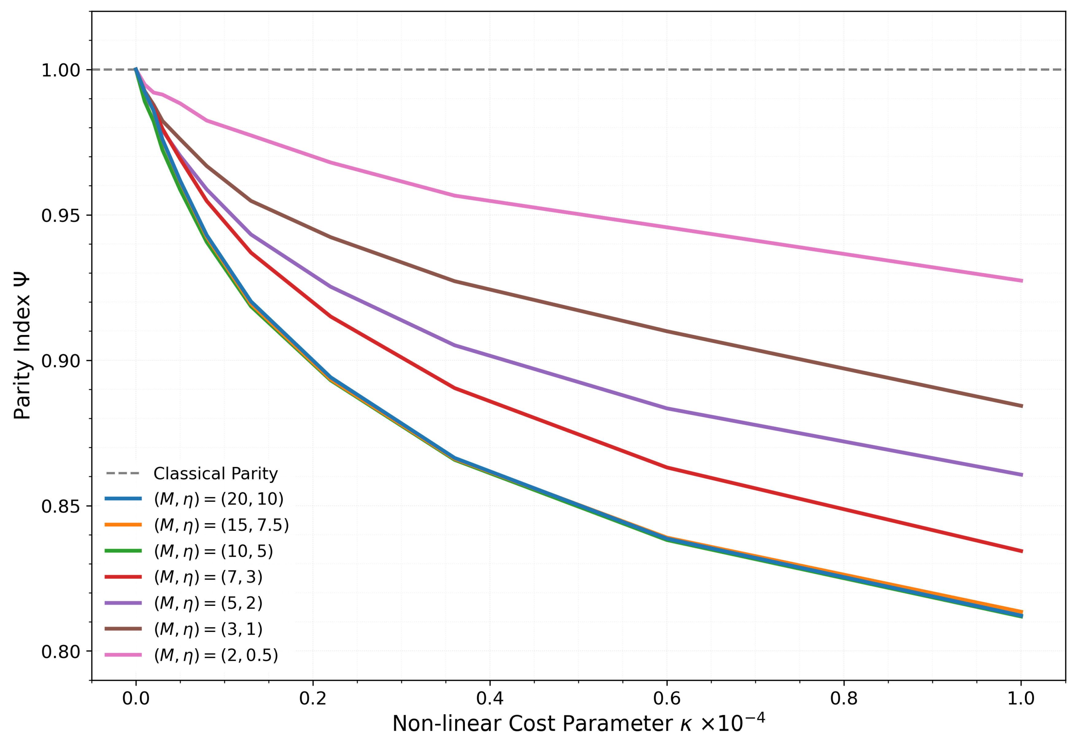
Figure 2.
Joint Effects across market environments: Parity Index in the two-dimensional parameter space of competition and non-linear costs (). Each panel shows a different market environment. The colour scale represents values, with blue indicating Adverse-Selection-Dominated regimes and red indicating Inventory-Dominated regimes . The black contour marks the classical parity boundary , showing where the two effects precisely balance.
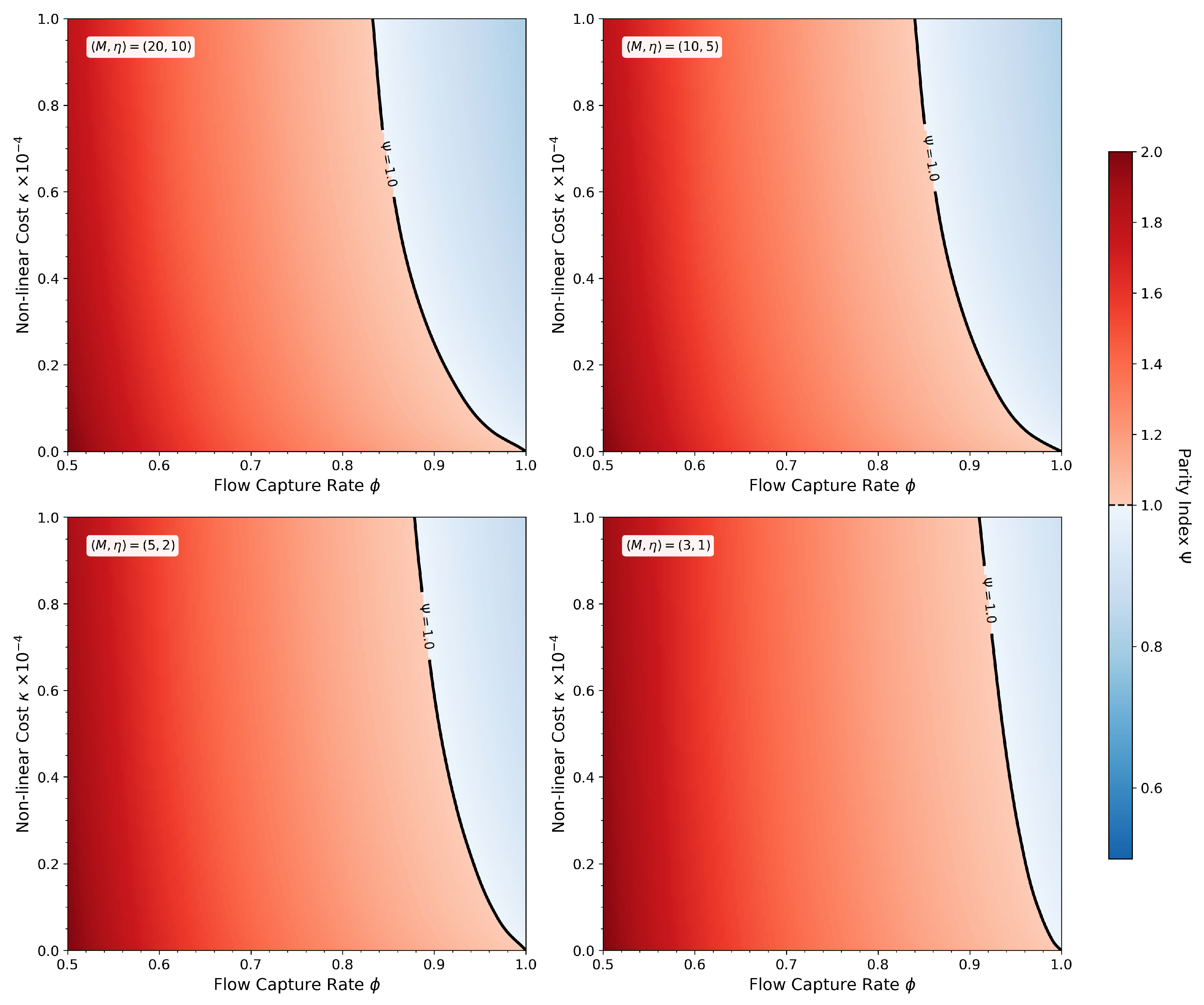
Figure 3.
Comprehensive analysis of adaptive behaviour effects across market structures and thickness levels. The 3×3 grid shows nine combinations (rows: monopolistic to fragmented competition; columns: linear to strong convex costs), with seven market environments plotted in each panel (from very liquid to very thin). Shaded regions represent 95% confidence intervals constructed using Rubin’s Rules pooling across simulation simulations. The systematic fan pattern reveals that liquid markets experience severe parity collapse while thin markets exhibit substantial resilience. The dashed horizontal line at marks classical parity.
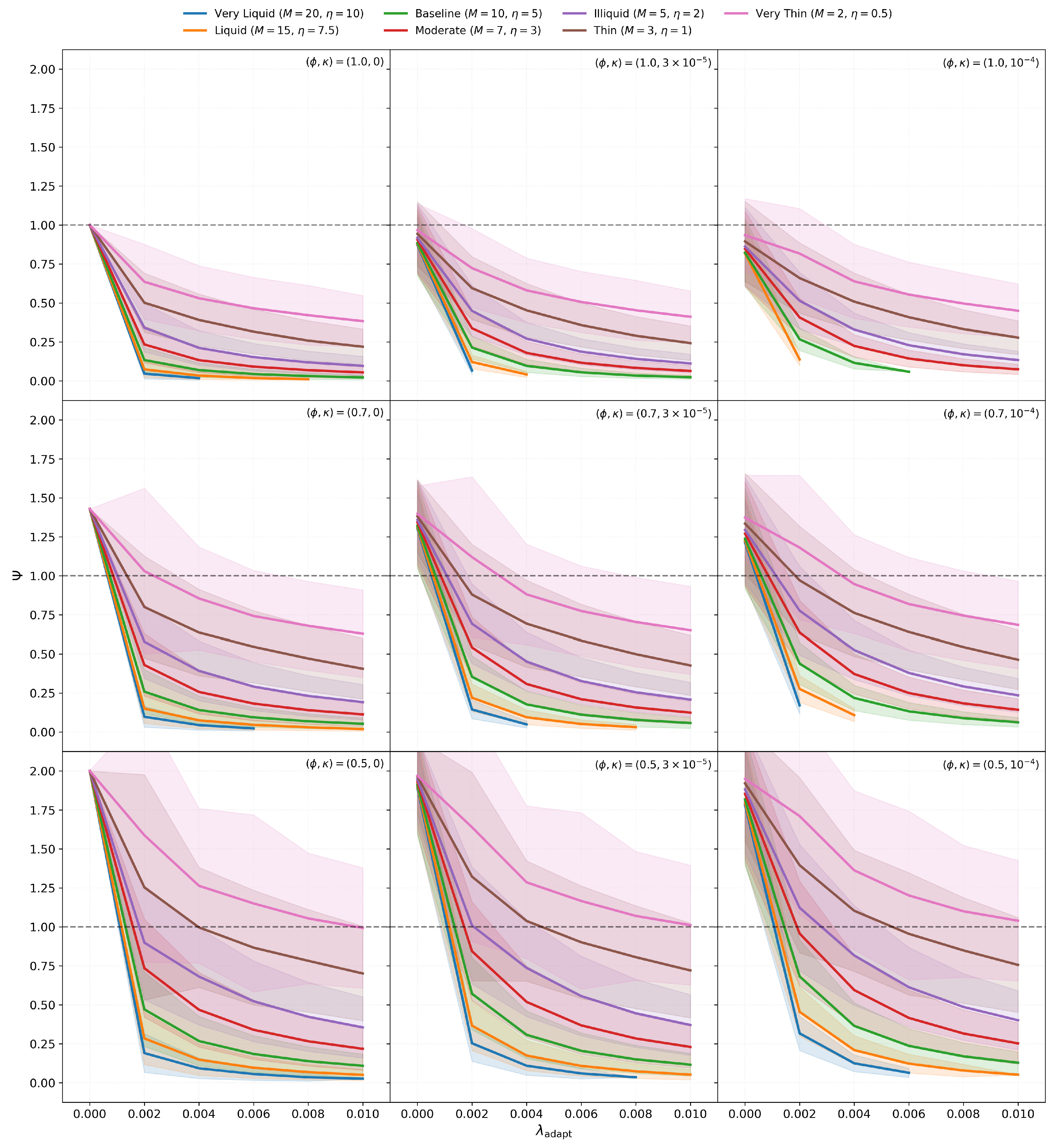
Figure 4.
Collapse factors across market thickness. Each line represents a combination, with colour indicating competition level (green=monopoly, orange=moderate, red=high fragmentation) and line style indicating cost structure (solid=linear, dashed=moderate non-linear, dotted=strong non-linear). Collapse severity increases strongly with market thickness M across all structural configurations, with monopolistic markets showing the steepest growth and fragmented markets the shallowest.
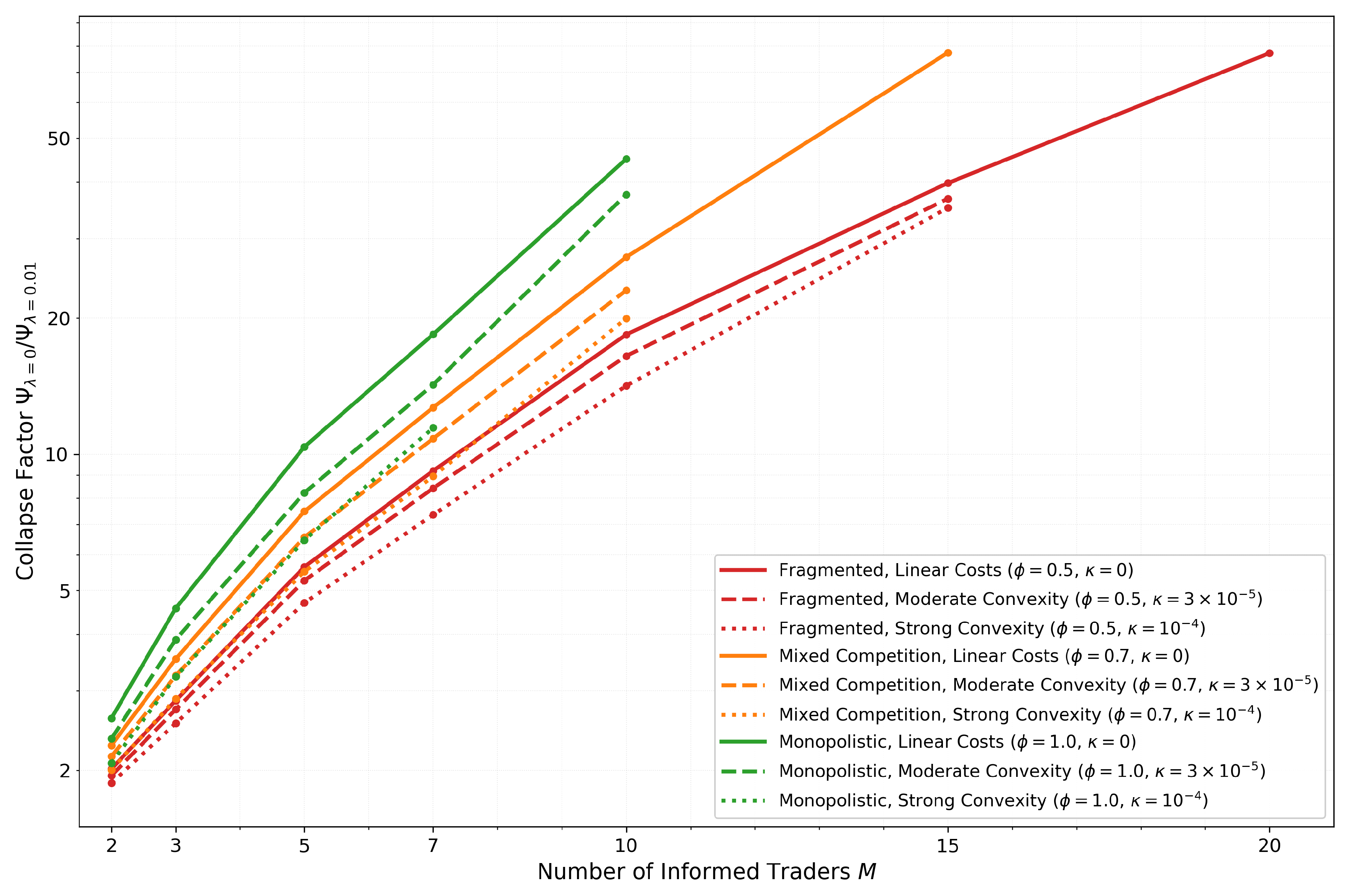
Figure 5.
Beta coefficient distributions across the full parameter space. The top panel shows the Kyle coefficient measuring information impact, with 97.8% of configurations (359,812 of 367,813) falling within empirically plausible bounds . The bottom panel shows the absolute value of the Ho-Stoll coefficient measuring inventory management, with 74.1% (272,432 configurations) satisfying bounds . The Ho-Stoll bound is the binding constraint on physical plausibility, with 269,182 configurations (73.2%) satisfying both criteria.
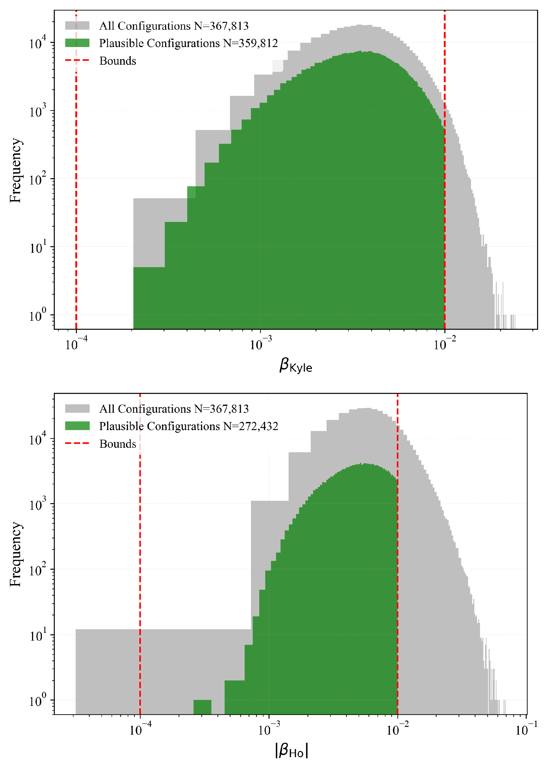
Figure 6.
Dual sensitivity analysis separating market fragility from performance attribution. The top panel presents first-order Sobol indices for the binary stability indicator, revealing that signal noise (), liquidity rate (), and informed trader count (M) contribute equally to market collapse risk with . The bottom panel presents Janon-Monod indices for the parity index conditional on stability, showing information quality () dominates regime variation with . Adaptation () could not be estimated due to zero valid configuration pairs, indicating threshold behaviour. Light-colored regions indicate interaction effects ().
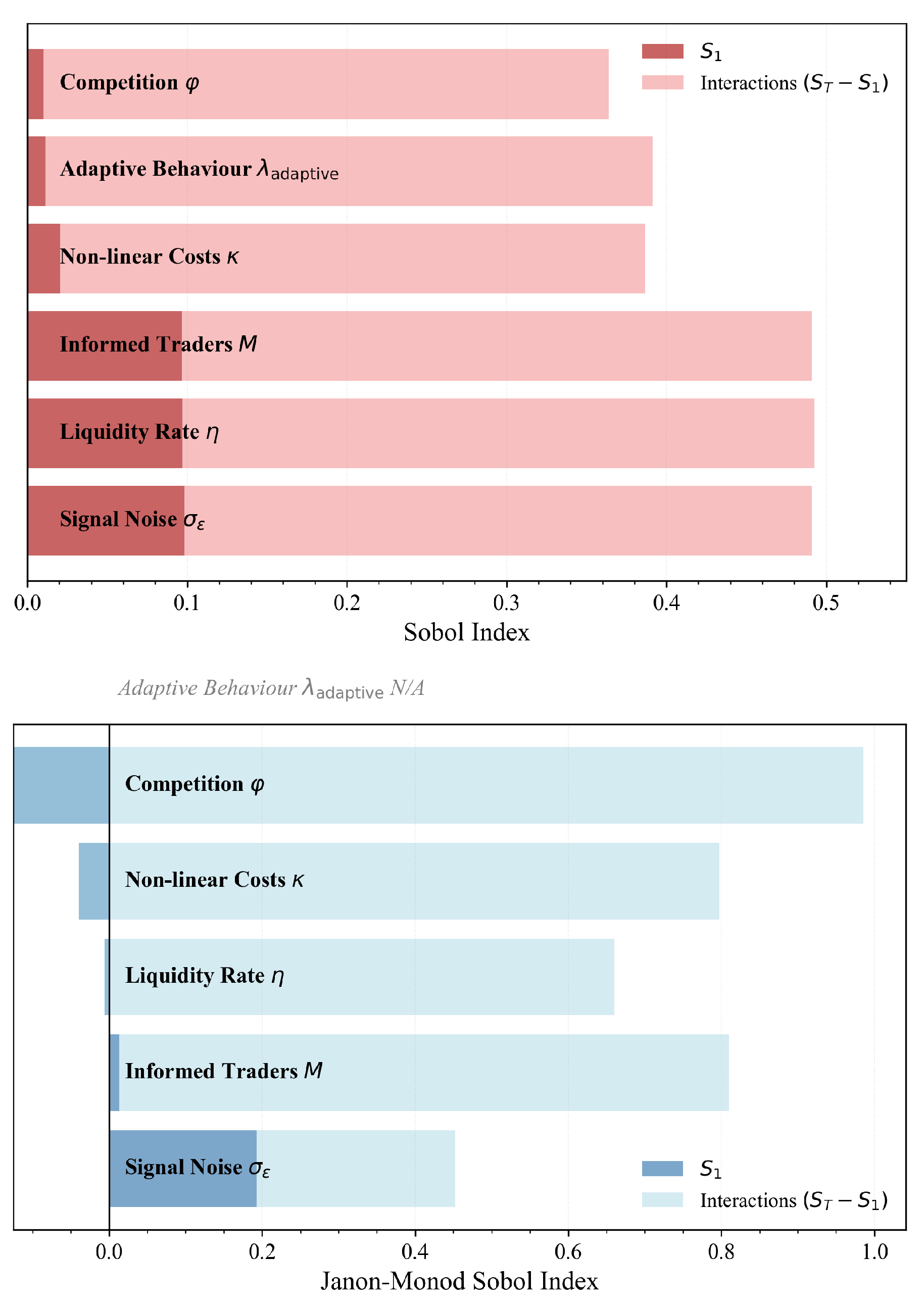
Figure 7.
Distribution and prevalence of market regimes. The top panel shows the parity index distribution in full parameter space (gray) versus physically plausible configurations (blue), with median values 1.875 and 1.643 respectively. Red dashed lines indicate regime boundaries at and . Right panel quantifies regime prevalence, showing inventory-dominated markets comprise 73.1% of plausible configurations, while adverse-selection regimes account for 18.5% and balanced-risk configurations represent only 8.4%.
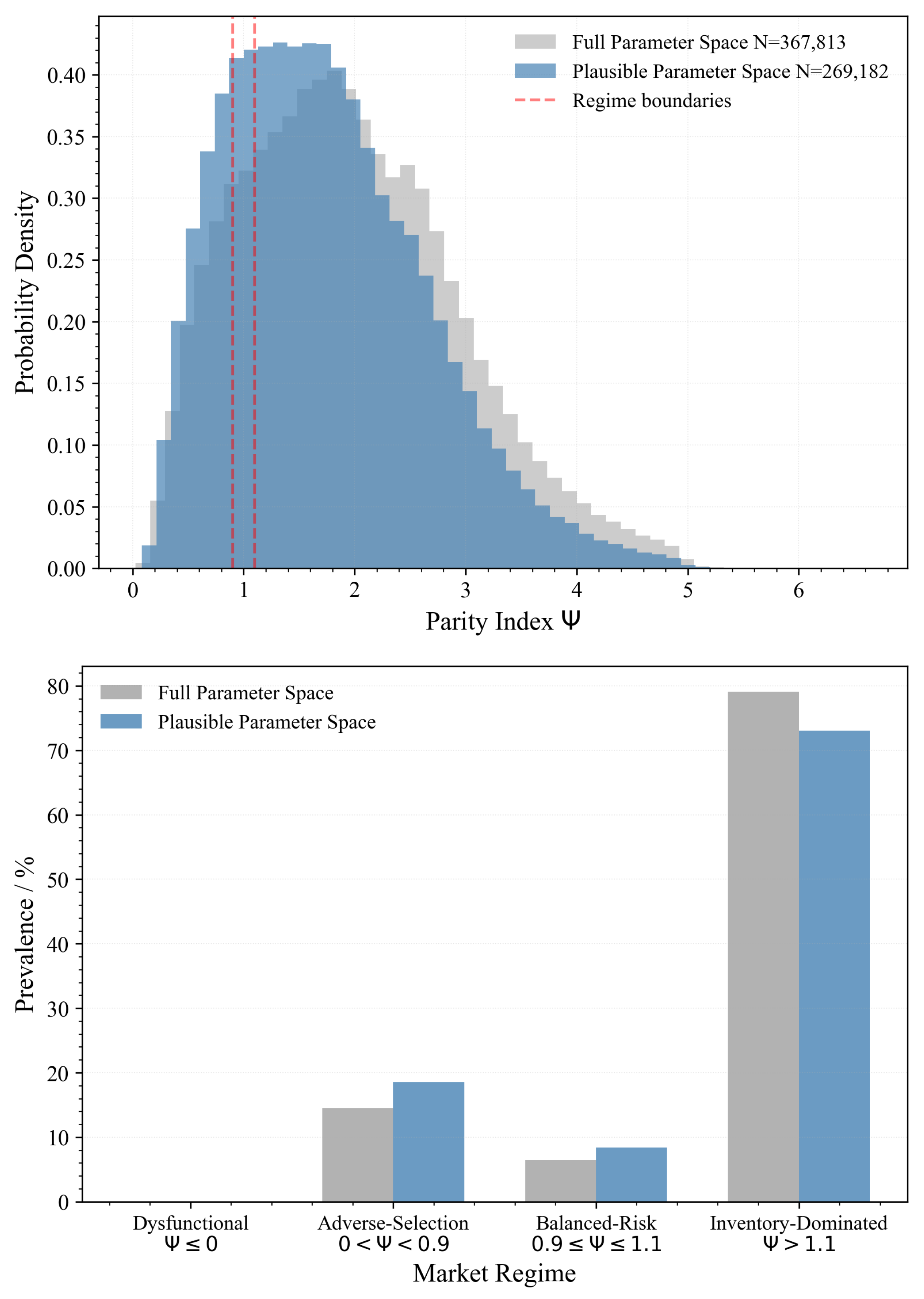

Table 1.
Baseline Simulation Parameters.
| Parameter | Symbol | Value |
| Environmental Parameters | ||
| Fundamental Value | V | 100.0 |
| Informed Traders | M | 10 |
| Liquidity Arrival Rate | 5.0 | |
| Signal Noise Std. Dev. | 1.0 | |
| Calibrated behavioural Parameters | ||
| Equilibrium Information Impact | 0.005 | |
| Baseline Inventory Aversion | 0.005 | |
| Equilibrium IT Aggressiveness | 0.1 |
Table 2.
Measurement reliability across market environments and all experimental conditions. Failure rates represent the proportion of simulation simulations (out of 1000 per configuration) excluded due to failed cointegration tests or stability filter violations. Mean statistics are averaged across all parameter combinations tested in the given market environment (including , , and variations); maximum values represent the worst-case configuration. values are computed from successful runs only.
| Market | M | Failure Rate | Failure Rate | |||
|---|---|---|---|---|---|---|
| (Mean) | (Max) | |||||
| Very Liquid | 20 | 10.0 | 0.003 | 0.014 | 0.948 | 0.884 |
| Baseline | 10 | 5.0 | 0.017 | 0.063 | 0.951 | 0.891 |
| Illiquid | 5 | 2.0 | 0.070 | 0.214 | 0.966 | 0.919 |
| Thin | 3 | 1.0 | 0.123 | 0.301 | 0.978 | 0.943 |
| Very Thin | 2 | 0.5 | 0.201 | 0.440 | 0.987 | 0.965 |
Table 3.
Parameter ranges for grid search and Sobol analysis. Initial ranges were explored via systematic grid search of configurations. Refined ranges, extracted from the 12.5% of grid configurations producing physically plausible coefficients, concentrate Sobol sampling within the dimensionally consistent thin market parameter space.
| Parameter | Symbol | Initial Range | Refined Range | Description |
| (Grid Search) | (Sobol Search) | |||
| Informed Traders | M | Market thickness | ||
| Liquidity Rate | Hedging intensity | |||
| Signal Noise | Information quality | |||
| Competition | Flow capture rate | |||
| Non-linear Costs | Inventory convexity | |||
| Adaptation | State-dependent behaviour |
Disclaimer/Publisher’s Note: The statements, opinions and data contained in all publications are solely those of the individual author(s) and contributor(s) and not of MDPI and/or the editor(s). MDPI and/or the editor(s) disclaim responsibility for any injury to people or property resulting from any ideas, methods, instructions or products referred to in the content. |
© 2025 by the authors. Licensee MDPI, Basel, Switzerland. This article is an open access article distributed under the terms and conditions of the Creative Commons Attribution (CC BY) license (http://creativecommons.org/licenses/by/4.0/).
Copyright: This open access article is published under a Creative Commons CC BY 4.0 license, which permit the free download, distribution, and reuse, provided that the author and preprint are cited in any reuse.


