
Submitted:
02 February 2025
Posted:
03 February 2025
You are already at the latest version
Abstract
We examine how short-sales policy regimes affect the efficiency of price adjustments and market stability. Using a ‘threshold error correction model’ (TECM), we find a more rapid convergence rate to new equilibria for upward adjustments than for downward adjustments. Moreover, relaxing the short sales constraints essentially improves price efficiency. Our findings refute the claim that tighter constraints can help stabilize the market since the tightening of the short-sales restriction leads to increases in both market volatility and downside risk. These results hold even when market conditions and liquidity are controlled. Even though prices may fall more sharply without short-sales bans, rather interestingly, the evidence from our counterfactual policy analysis suggests that tighter constraints help restore market confidence. As a result, policymakers may practically optimize to strike a balance between the benefits of restored market order and the cost of elevated market volatility.
Keywords:
Short Sale Constraints
; Price Efficiency
; Put-call Parity
; Threshold Error Correction
; Counterfactual Policy Analysis
1. Introduction
Given the recent financial crisis, academic researchers, market practitioners, and regulators are keen to understand better the highly contentious impact of short-sales policies on stability and pricing efficiency within capital markets. Stock exchanges and government supervisory bodies have found it difficult to reach any consensus on a consistent set of short-selling guidelines. As a result, short-sales regulations continue to vary widely across countries and capital markets (e.g., Bris et al., 2007). While researchers have generally found that short-selling constraints (hereafter referred to as SSCs) will lead to a more volatile market,1 in contrast to the argument from Franklin and Gale (1991), the reality appears as an empirical puzzle since most regulators have resorted to imposing SSCs when their markets are drastically volatile.
To resolve this puzzle, we investigate whether SSCs play a role in stabilizing a market when it is fragile. As the ability to short-sell affects liquidity and the adjustment toward new market equilibria, we seek to disentangle the effect of SSCs on price discovery and market efficiency. Miller (1977) and several recent studies2 on the relationship between short sales and stock overvaluations3 have shown that the SSC may result in overpriced securities and low subsequent returns. This, unfortunately, may be due to the lack of transaction data or models that were able to characterize the speed of price adjustments in the past and, until recently, had seldom been used to examine price adjustments in response to new information. For example, Chen and Rhee (2010) present empirical evidence to show that short sales on the Hong Kong Exchange contributed to market efficiency by increasing the speed of price adjustment for private/public firm-specific information and market-wide information.
In a departure from the existing literature, we examine the effects of SSCs on both the speed of price adjustment to the new equilibrium and market stabilization within a properly identified threshold error correction model (TECM). By taking advantage of the changes in short-selling policies implemented between 2002 and 2009 in the emerging Taiwanese market, our study provides several empirical insights based on price discovery within a series of “natural social” experiments. The beauty of the model used in the context of different regimes is that we can perform direct counterfactual analysis to assess “what if” scenarios when disentangling the policy effects of SSCs.
From an equilibrium perspective, if the restrictions on short sales hinder price discovery in the underlying spot index, investors can alternatively short-sell, at an even lower cost, by writing puts or shorting calls in the options/futures markets4. Voluminous empirical results have suggested that the options market plays a more informative price discovery role, especially when short selling is restricted in the spot market. Therefore, we use the put-call parity derived index, free from model misspecifications and biased volatility inputs5, as a proxy for the virtual price equilibrium. We explore dynamically how mispricing is adjusted towards the new equilibrium through this cointegration linkage between the spot and derivative markets. The analysis of the effects of SSCs on adjustment speed is straightforward and uses a comprehensive TECM approach. More importantly, unlike the extant literature that employs daily or monthly data, our study hinges on the 1-minute high-frequency equilibrium deviations to resolve the issue of market efficiency adjustment and issues about market stability under SSCs. These are all highlighted as the major differences between our study and those in the recent literature.
Our main findings are as follows. First, we find that tighter SSCs help to retain investors’ confidence, effectively discouraging the execution of “fire sales” and saving the market from liquidity “droughts,” as verified by our counterfactual analysis of the realized equilibrium adjustments. However, tighter constraints provide little help in stabilizing market fluctuations, which are generally associated with greater downside risk and higher volatility. Specifically, our robustness check reveals that these results hold, even after controlling for the investor “fear index”' or “fear gauge,” which is proxied by VIX in our study. Secondly, in the presence of mispricing, short sales constraints lead to a less efficient market by creating asymmetry in both the magnitude and speed of price adjustments. Within our TECM, the convergence rate of upward adjustments is more rapid than that of downward adjustments, even after controlling for market conditions and liquidity. Finally, the speed of downward adjustments significantly improves after the relaxation of such constraints.
Our empirical results shed practical light. The market is fragile during the financial crisis as the market liquidity critically depends on investor confidence. The consideration of flying to safety/liquidity can further amplify the contraction of funding liquidity through the unwinding and deleveraging of positions among various market participants. Given that a loss of confidence can trigger fire sales and destabilize the financial system, the SSCs, as a policy tool, can be used to protect against these undesired scenarios. Policy-makers may then take advantage of the SSCs by optimally striking a nice balance between the cost of obstructing price efficiency and the benefits of restoring investor confidence, mainly when it is scarce during a financial crisis.
The remainder of this paper is organized as follows. A description of the data and short-sales policy changes in Taiwan is presented in Section 2, followed in Section 3 by developing our hypotheses and empirical design. Section 4 presents our main empirical results along with a counterfactual analysis. Various robustness checks are provided in Section 5. Finally, the conclusions drawn from this study are presented in Section 6.
2. Data and Description of Short Sales Policies
It can be empirically difficult, if not impossible, to identify the policy impacts of SSCs since the durations of SSCs policies implemented are often too short for meaningful examinations of the policy consequences, even for some specific developed countries. However, the experience of Taiwan provides an interesting avenue for research, as a ban on short selling in terms of the up-tick rule was superimposed in Taiwan over a long period.
The data analyzed in this study are intraday TAIFEX index options and their common underlying asset on the Taiwan Stock Exchange Capitalization Weighted Stock Index (TAIEX), details of which are available from the Taiwan Economic Journal (TEJ) database. We chose the TAIEX index because the institutional factors within the Taiwanese market closely resemble a representative case of an emerging market with its large population of retail investors, heavy government intervention, and regulatory controls. These institutional factors are distinctly different from those in the markets of developed countries. Therefore, the impacts of such SSC policy adjustments toward market efficiency and stability are of practical relevance and informative for many emerging and developing economies.
2.1. SSCs Policy Changes
The Taiwan Stock Exchange (hereafter TWSE) initially imposed an up-tick rule in September 1998, which allows short selling only at prices that are at least as high as the closing price for the previous trading day for all stocks eligible for short sales.6 In an attempt to improve the efficiency of price discovery, the TWSE relaxed the up-tick rule on June 30, 2003 for equities listed in the first exchange-traded fund (ETF), the Taiwan Top50 Tracker Fund (TTT ) (ID: 0050). Starting May 16, 2005, the component stocks of TTT were allowed to freely short sell. 7 Therefore, we have the following three periods: p1, from January 2, 2002 to June 29, 2003; p2, from June 30, 2003 to May 15, 2005; and p3, from May 16, 2005 to November 11, 2007. Starting November 12, 2007, the constituent stocks of the Taiwan Mid-Cap 100 index and the Technology Index were also exempted from the uptick rule. As a reaction to the global financial crisis, from September 22, 2008 to the end of that year, the TWSE banned the short selling of 150 companies’ shares below their closing prices on the previous day, which marks our fourth and fifth sub-periods as p4, from November 12, 2007 to September 21, 2008, and p5, from September 22, 2008 to December 31, 2008. It should be noted that the regulators imposed a further ban on the short-selling of all stocks from October 1 to November 27, 2008, prohibiting all short-selling during that period. Finally, p6 denotes the relaxation of all SSCs from 2009 onwards. Beginning September 23, 2013, around 1,200 borrowed stocks currently eligible for margin trading have been exempted from the up-tick rule and can be sold at a price lower than the closing price on the previous trading day.
As our sample period runs from January 2002 to December 2009, we have divided the entire sample period into six sub-periods according to these short-sales policy changes (see Figure 1). The strength of the SSCs throughout the various periods, from the highest to lowest, was in the order of p5, p1, p2, p3, p6 and p4.8 Thus, these policy changes provide us with natural proxies for examining the effects of the SSCs on market stability and market efficiency.
2.2. SSCs Proxies
Most previous empirical studies related to SSCs rely either on various measures to characterize the strength of SSCs or on restricted samples with lending data. The former includes a variety of proxies that have been used for capturing higher SSCs or higher short-sales costs9; the latter stream uses lending data provided by one or some custodians10. Saffi and Sigurdsson (2011) once argued that the loan fee represented the average lending price11. However, it could be challenging to collect complete data from all custodians, and since we can never know whether custodians have different pricing strategies, such data may not be at the equilibrium lending price.
As suggested by Diether et al. (2009a) and Saffi and Sigurdsson (2011), it is difficult to determine whether high short interest reflects either negative sentiment amongst investors regarding the stock or lower SSCs. As Diether et al. (2009a) have further argued that short sellers will quickly cover their positions, the monthly short interest would be inappropriate for addressing the short-term adjustments toward a new equilibrium. These shortcomings can be avoided through the use of better proxies for SSCs. Fortunately, the short-sales policy changes in Taiwan between 2002 and 2009 provided a natural platform for examining how the market equilibrium responds to the various SSCs regimes. Our paper addresses how the market reacts to SSC policy changes.
2.3. The Implied Index Price and Equilibrium Deviations
The theoretical index price obtained in this study is based upon put-call parity12, a simple no-arbitrage relationship for which there are no superimposed assumptions regarding agents' preferences or return distributions (Chiou et al., 2007). In the absence of arbitrage opportunities, the put-call parity suggests that the implied index price be given by
where () denotes the call (put) price at the time for an option contract maturing at; is the synthesized implied price as a proxy for the equilibrium price; is the risk-free rate; and represents the strike price.
Given the current price index, we have collected seven series of near-month option contracts with different moneyness.13 To remove the effect of different moneyness, we then average the seven implied index prices over their moneyness to arrive at the final theoretical index price (StO ) for time t. Intuitively, the logarithmic observed index value and the put-call-parity implied theoretical index are cointegrated with their common trend discernibly depicted in Figure 2a, and the formal cointegration test results are provided in Table 1.
It is interesting to explore why the positive deviations between the index price and theoretical index price became larger during the short-sales ban period (as we can see from Figure 2c and Figure 3a) and whether the regulators imposed such constraints to stabilize prices whilst witnessing greater fluctuations in returns, as illustrated in Figure 2b.
Our sample period runs from January 2, 2002 to December 31, 2009, yielding 1,989 days and 539,109 one-minute intraday observations. We use high-frequency data instead of previous empirical studies that employed low-frequency data because the empirical results find that short sellers covered their positions within a few days14.
Utilizing data at a lower frequency may fail to resemble the equilibrium adjustment and hinder the price discovery occurring at a higher frequency. In the present study, we find that the average time taken to converge to equilibrium in the examined Taiwanese market between 2002 and 2009 was, on average, 26 minutes. Secondly, given that there is a high proportion of day trading activities and high turnover in the Taiwanese market, only high-frequency data may help reveal the nature of equilibrium adjustments and efficiency changes, particularly during periods of exogenous policy changes.
2.4. Other Variables and Control Variables
Using high-frequency data avoids the potential problem of non-synchronous trading confounding the results, whilst index-level analysis undertaken at a market-wide aggregate level can help avoid idiosyncratic risk and analyst disagreement15. Given the potential link between price movements and other variables, such as liquidity, transaction costs, market conditions, and the microstructure effect, it is essential to control alternative concerns properly.
A total of five measures are employed to control for the effects of market liquidity16 on price movements: (i) Num_Trades is the number of trades in the previous minute; (ii) Num_Shares denotes the number of trading shares in the previous minute; (iii) TDollart–1 denotes the amount of trading in the previous minute (in dollars x 1,000); (iv) Daily_Turnover is calculated as the trading volume on the previous day divided by the number of outstanding shares on the previous day; and (v) Daily_Turnover/MV denotes the daily trading dollars divided by the daily market value (Saffi & Sigurdsson, 2011). As we can see from Table 2, the market is more liquid during periods when SSCs are lifted.
We also use 5 different measures to resemble the market condition. The daily one-minute index returns are calculated by the average return, skewness, kurtosis, and standard deviations calculated from the one-minute index returns over the previous three-month period. The variables capture the heavy tail phenomena in the index returns, whilst the average market returns over the previous three-month period capture how bear or bull markets affect price movements. and capture the daily index price variations and volatility variations during different SSC periods (Table 2).
Jiang et al. (1996) deleted their sample's first ten-minute data segments as investors could have been overreacting to overnight news releases. Since the present study focuses on intraday return behavior, an overnight dummy variable (identifying transactions occurring at 9:00 a.m.) is included in our model to control for the overnight effect on price movements. In their analysis of the impact of the short-sales price test pilot plan on market quality in the US, Diether et al. (2009b) excluded data from 9:30-10:00 a.m. to avoid the undue influence of the market opening in their results. Following their merits, we also include open and closed dummies for control in this study, where Open (Close) equals 1 if the transactions occurred during the 9:01-9:30 (13:01-13:30) period.
3. Hypothesis Development and Empirical Design
Most of the previous theoretical or empirical studies looking at the policy effects of SSCs are concerned with the magnitude of price changes17. However, few studies have examined the speed of adjustment towards the fundamental price18. This paper seeks to fill this gap.
To see this, we define the price deviation as the natural logarithmic difference between the index price and the theoretical index price as the error-correction term representing the possible arbitrage opportunities19:
An overvaluation emerges when the spot price is higher than the theoretical price. The unconditional adjustment periods in our preliminary results exhibit a discernible asymmetric pattern between upward and downward adjustments, with an overvaluation taking from 27 to 86 minutes to converge to equilibrium during the period with the fewest SSC, as compared to just 11 to 16 minutes to equilibrium for an undervaluation20 during the period with the strongest SSC, after considering the transaction costs21.
3.1. Improved Speed of Price Adjustment
To illustrate the different effects on upward and downward price adjustments, we specifically employ the threshold error correction model (TECM) 22 with varying rates of upward and downward adjustment to identify whether any asymmetric patterns exist in the convergence speed. The TECM specifies the magnitude of the deviation from the theoretical price that will ultimately trigger trading and provides possible estimates for explicit and implicit transaction costs, which may prevent investors from adjusting immediately (Dwyer et al., 1996). From a financial standpoint, we also care about the extent to which the deviations may be sufficiently large to cover the total costs incurred by investors, including transaction costs and risk. The nonlinear flexibility to estimate the latent decision thresholds in a TECM allows us to capture the market frictions, such as transaction costs, the tax burden, and market microstructure.
We set out to characterize market friction and price adjustments in terms of a more general three-regime TECM. The threshold values (, ) are estimated by following the approach of Enders and Siklos (2001) and Balke and Fomby (1997)23. The three-regime TECM is estimated using the thresholds and :
where () refers to the speed of downward (upward) adjustment for and, as far as possible, with all transaction costs (such as ). Refers to the speed of adjustment in the interband. It is the error correction term, and the coefficient specifies the speed of adjustment towards the theoretical price, and it should be negative. And denote the zero-mean, serially uncorrelated error terms, which may be contemporaneously correlated, and refer to the control variables (including market liquidity, market condition, and market microstructure). We examine Hypothesis 1a, which states that the adjustment speed will be more rapid for upward adjustments.
Hypothesis 1a:
Upward adjustments are more rapid than downward adjustments under general SSC.
When the SSC binds, assets can be overpriced due to the SSC impeding arbitrage activities by the pessimistic traders. As a result, the adjustment period for an overvaluation should be extended. By analogy, the market will exhibit a slower downward adjustment under a tighter SSC. Given the disclosure of a significantly different adjustment period for overvaluations but no significant differences for undervaluations between the weakest and strongest SSC intensity (and periods) in our preliminary results, we proceed to examine whether the slower speed of price adjustment is more pronounced at the time in which short sales are prohibited; and if price efficiency improves during periods of relaxed SSC as noted in Section 2.2.
We define (and ) as the average downward adjustment speed during strict (and relaxed) SSC. We go on to extend our three-regime TECM with downward (upward) adjustment speed under the various policy changes to examine the adjustment speed between the weakest () and strongest () levels of SSC with the estimated thresholds and as follows:
where () is the downward (upward) adjustment speed, taking all transaction costs into account under the various policy changes ( and ). The other notation follows previous definitions.
The three-regime TECM enables us to specify what size deviations from the theoretical price will trigger trading and resolve the puzzle of how SSC affects market efficiency. If the SSCs suppress the realization of lousy news in prices, one would expect market efficiency to improve when the SSCs are relaxed, i.e., the speed of the rigid downward adjustment to new information will be more rapid. Therefore, we construct our Hypothesis 1b as follows:
Hypothesis 1b:
The speed of downward adjustment will increase due to the relaxation of SSCs.
3.2. Price Stabilization under SSCs: A Counterfactual Analysis
To shed light on the remaining puzzle regarding the short-selling policy and market stabilization, i.e., why the regulators still employ academically vicious SSCs for stabilization, we conduct an informative counterfactual analysis to see what would happen where the SSC policy is not launched (or with zero-SSC). Recall that the option-implied theoretical price is free from SSCs. Therefore, the theoretical price should be least affected by the short sales ban, and only the index price should be adjusted in cases of a short sales ban. We follow Politis and Romano (1994) and Hsu, Hsu and Kuan (2010) to examine whether the market price may have fallen even further without the short-sales ban based upon a counterfactual simulation and stationary bootstrap method. As the speeds of adjustment across different levels of SSC intensity are well estimated in our adopted TECM model, we simulate the market price without the short-sales ban and then examine whether the price with the short-sales ban could mitigate the price fluctuations.
Hypothesis 2a:
The price without a short sales ban may drop more than that with a short sales ban.
Short-sales activities are arguably an important element of any discussion on market stabilization. Regulators claim that short selling is detrimental to price stabilization. However, the academic evidence indicates that stocks with fewer SSCs have lower kurtosis (see Saffi and Sigurdsson, 2011), along with lower levels of both downside risk and total volatility. Since our high-frequency data allow us to calculate the characteristics of the distribution of the daily index returns, we can test our hypothesis by examining the differences in the characteristics of the index return distribution, under the various policy changes and then go on to provide some suggestions for regulators about short sales:
Hypothesis 2b:
Tighter SSC, or a total ban on short sales, will not enhance the price stabilization.
4. Empirical Results
4.1. Rapid Upward and Sluggish Downward Adjustment
Compared with all other periods, the price deviations are more than three times greater during the strictest constraint period24 (see Table 2). As noted earlier, these policy changes, from the highest to the lowest intensity of SSCs, are in the order of. By taking advantage of a hybrid of high-frequency data, the natural experiments, and the TECM approach, this paper addresses the gap in prior studies by characterizing how and by how much the SSCs affect market efficiency. Under no-arbitrage pricing, prices will adjust immediately after their initial departure from the fundamental value of the asset; thus, theoretically, the duration of upward adjustments should be exactly the same as that of downward adjustments.
Diamond and Verrecchia (1987) and Hong et al. (2000) noted that SSCs delayed the effects of negative news on the price; that is, SSCs impede the propagation of bad news, with the cumulative negative momentums being too heavy to bind, which may potentially lead to a total collapse or a bubble (Hong & Stein, 2003; Lim, 2011). Conversely, relaxing restrictions improves the dissemination of downside news disclosures.25
In order to specify how much SSC delayed the effects of negative news on the price, we construct the three-regime TECM with market friction items controlled in Equation (3). That is, the estimated thresholds represent the barrier to trade that is necessary to cover all transaction costs. Following Enders and Siklos (2001), the threshold values and threshold lags (denoted as )26 are obtained from the minimum mean squared error of the TAR model.
Since the speed differences between upward () and downward () adjustments are significant in Table 3, we can conclude that the speed of an upward adjustment to the new equilibrium is much more rapid than that of a downward adjustment, even after controlling for as much market friction as possible. These results provide strong support for Hypothesis 1a. This finding is similar to that of Miller (1977) and Shleifer and Vishny (1997), who identified illiquidity risk and SSCs as impediments to arbitrageurs entering and trading in the spot market, so when seeking to determine the cause of longer periods of adjustment they did so only in those cases where the spot market was overvalued27. The results confirm that SSCs hinder the speed of incorporating bad news into the price more than 6 times that of good news. In this case, we conjecture that the speed of downward adjustment will improve adjusting periods when the constraints are lifted, as compared to during those periods with the strictest constraints. Next, we focus on market responses to the arrival of bad news under different levels of SSCs.
4.2. How is Market Efficiency Improved after Lifting SSCs?
We further examine if the speed is improved for downward adjustments after the SSCs are lifted. Since the downward adjustment speeds between the lowest ( ) and highest () SSCs intensity are significantly different as shown in Table 3, our Hypothesis 1b is strongly supported. To put it differently, interestingly, our results indicate that the relaxation of SSCs has accelerated the speed of downward adjustment by up to more than 2.7 times its original speed. In other words, lifting SSCs indeed enhances market efficiency.
4.3. Counterfactual Analysis of a Zero-SSC Scenario
In this subsection, we further try to resolve the remaining puzzle---why policy makers implement SSCs that may deteriorate market efficiency under a market crisis. The results above have shown that tighter SSCs actually give rise to market inefficiency in an asymmetric manner, as the downward adjustment is much slower, particularly during the period when short sales were banned. Nonetheless, if we interpret the evidence from the other perspective, a slower response to bad news seems to provide justification for stabilizing market fluctuations since slower downward adjustments may lead to complacency among investors in terms of market confidence. Despite such an argument appearing to be indirectly supported by several studies that note that financial bailouts can mitigate a credit crunch problem, the related costs are huge.28 To assess the likely state of the market index in the absence of the SSCs or ban, we implemented our counterfactual simulations with a stationary bootstrap algorithm, as shown in the procedure in Appendix A. The time-series plot for the price differences between the true market index with the short-sales ban and the pseudo-true index without the short-sales ban is now illustrated in Figure 4.
The first and second pairs of dashed lines denote the start and end dates of the short-sales ban on all equities during the period from October 1 to November 27, 2008. The positive difference between the true and pseudo price indices indicates that the short-sales ban succeeded in halting falling prices. As we can see from Figure 4, almost all of the price differences are large and positive during the total short-sales ban period, whereas less positive price differences are discernible in periods when short sales were only prohibited under up-tick rules. Therefore, we conclude from our counterfactual analysis that SSCs are helpful in quelling concerns among investors and preventing the execution of fire sales while also avoiding liquidity ‘droughts’ in the market during a short-sales ban.
4.4. Tighter Constraints, Higher Risk and Price Fluctuations
Our empirical analysis in Table 4 has declined in that the SSCs lead to a more stable market since tighter SSCs are associated with higher total risk and downside risk. As such, while SSCs have failed to achieve the regulators’ purpose, several studies disagree with the perspective that short selling is detrimental to price stabilization.29 We thus proceed to reexamine the characteristics of the index return distribution and spot market risks affected by SSCs changes to provide insights for regulators.
Consistent with the evidence presented by Bris et al. (2007), skewness is reduced with tighter SSCs. We also find that kurtosis is increased under such strengthened constraints, which is consistent with the findings of Saffi and Sigurdsson (2011). We, therefore, conclude that tighter SSCs are associated with both lower skewness and higher kurtosis30.
() denotes the magnitude of the daily occurrence of extreme negative (positive) returns, defined as index returns that are less than (greater than) two standard deviations during each period of policy changes. Reading through the relevant columns, we failed to find clear evidence of short sales increasing either the frequency of extreme returns or the likelihood of a market crash.
the sum of the squared daily one-minute index returns represents the realized semi-variance (the sum of the squared negative returns). As shown in the last two columns in Table 4, higher SSCs are positively correlated with total and downside risk, where the results largely echo those of Charoenrook and Daouk (2005). Overall, there is no evidence of tighter SSCs being associated with enhanced price stability; on the contrary, the imposition of such SSCs is generally associated with a reduction in pricing efficiency and an increase in downside risk.
5. Robustness Checks
5.1. Further Evidence on High Short Demand Transactions
If there are indeed some transactions in the stock market with high short demand, then the adjustment speed of such transactions should be much more rapid during periods when the constraints are relaxed. We follow Fung and Jiang (1999) and Jiang et al. (2001) to measure market direction using the ‘relative strength index’ (RSI) in order to identify the direction of the price movements; they defined the highest 10th percentile of RSI as transactions with ‘high short demand’.
where () is the daily number of one-minute intervals in which the TWSE spot index advanced (declined).
Our observations are sorted into ten deciles, based on the daily RSI, with the highest decile representing the most positive price movements, thereby indicating a period when short selling is more likely. We define the highest 10th percentile of the RSI as the period most likely to attract short selling, which is denoted in this study as a ‘high propensity to short’ (hereafter as HPTS).
We aim to identify whether the relaxation of constraints accelerates the rate of downward adjustment for HPTS; that is, whether the absolute value of exceeds that of based upon the estimated threshold value above. Next, we examine the model with varying upward and downward adjustment rates in cases of HPTS with different constraint pressures, which is expressed as follows:
where and denote the indicators for overvaluations and undervaluation with those transactions under different SSCs policies; denotes the speed of downward adjustment in the case of transactions with HPTS, for, and the other notation follows the previous definitions.
The results support our hypothesis 1b. In Table 5, we have witnessed the fact that the relaxation of SSCs promotes more rapid downward adjustment for transactions with high short demand. We also find evidence supporting Hypothesis 1a in that the speed of adjustment is asymmetric, with the pace of upward adjustment being more rapid than that of downward adjustment, even in the case of HPTS. The high short-demand transactions are divided into six groups according to the policy changes to verify whether the lifting of constraints might speed up the convergence rate toward equilibrium31. The results deliver similar conclusions.
5.2. The Elevated Risk Due to Stronger SSCs
The question arises as to whether the increases in downside and total risk in the 2008 financial crisis period resulted from the tightened SSCs or simply due to the increased market volatility. To tease out the endogeneity from the higher market volatility, we specifically regress the and on a set of dummy variables characterizing different SSCs regimes as well as the TAIEX VIX32 index as a hybrid control variable for market-wide sentiments and volatility during this period.
As shown and expected in Table 6, the VIX index significantly positively comoves with the risk measures examined. Surprisingly, while controlling for market-wide sentiments and volatility, the significant positive estimates for the p5 regimes in both regression equations suggest that tighter SSC intensity indeed positively contributes to both the escalated downside risk and total risk. The marginally imparted greater downside risk and higher volatility due to tighter SSCs are non-negligible, even after controlling for the investor fear gauge, proxied by VIX.
6. Conclusions
The regime shifts in the regulatory uptick rules in Taiwan between 2002 and 2009 provide a sequence of natural experimental environments to examine the stock market responses to short sale policy changes. Our research arrives at three main empirical findings.
First, in the presence of mispricing, SSCs lead to a less efficient market by delivering asymmetries in the magnitudes and speed of price adjustments. Consistent with the prior studies, such constraints are generally found to hinder the reflection of negative information in the price; thus, based on the TECM adopted for this study, we document that upward adjustments converge more rapidly than downward adjustments, even when controlling for market conditions and liquidity. Secondly, we find that the speed of downward adjustments is improved in periods characterized by relaxed SSCs. Finally, the realized equilibrium adjustments identified through our counterfactual analysis also indicate that SSCs can indeed restore investor confidence, thereby discouraging the execution of fire sales and saving the market from further liquidity problems. However, we find that such restrictions are of very little help with regard to stabilizing market fluctuations. In particular, stricter short-sales restrictions are associated with greater downside risk and higher volatility.
Our results hold, even after controlling for the investor fear gauge, which is proxied by VIX in this study. Interestingly, however, our findings provide clear support for the academic finding that short-sale constraints generally lead to a less efficient market. Even though there is no evidence suggesting that regulators can stabilize prices by restricting short sales, it is truly likely that such policy announcements may retain/restore investors’ confidence, which is a valuable yet scarce resource especially when markets are plunging.
Author Contributions
Conceptualization, Lin Kun Chan; Data curation, Lin Kun Chan; Formal analysis, Lin Kun Chan; Investigation, Lin Kun Chan; Methodology, Lin Kun Chan; Project administration, Chin Yang Lin; Resources, Lin Kun Chan and Chin Yang Lin; Software, Lin Kun Chan; Supervision, Jin-Huei Yeh; Validation, Lin Kun Chan; Writing – original draft, Lin Kun Chan; Writing – review & editing, Lin Kun Chan and Chin Yang Lin.
Funding
This research received no funding.
Appendix A. Counterfactual Simulation Analysis with a Stationary Bootstrap
We follow Politis and Romano (1994) and Hsu et al. (2010) to examine whether the market price may have fallen even further without the short-sales ban based on a counterfactual test and stationary bootstrap method. We simulate the market price without the short sales ban and then compare whether the price with the short sales ban could mitigate the price fluctuations. The simulation with a stationary bootstrap algorithm is computed as follows.
1. Start with the residuals in Equation (4) during the short-sales ban period {ε1j,…, εTj }, where T = 19241 and.
2. Let {ub,t}tT =1 be a randomly drawn i.i.d., with uniform distribution within the set {1, 2 ,…, T}, representing the starting points of the new blocks.
3. Let {vb,t}tT =1 be a randomly drawn i.i.d. of continuous uniform distribution with domain value (0,1], representing the resampling probability.
4. Start with τb,1= ub,1. For any t >1, the bth resample of εtb = ετb,1,
where τb,t =. A resample, εtb, is carried out when T observations are drawn.
5. The speed of adjustment and the estimated threshold are then used to calculate until observations are included. A simulation of the price series without the short-sales ban is duly completed. We assume that the speed of adjustment and the estimated threshold in Equation (4) will be the same as those if the short-sales ban is not executed during.
Repeating this procedure yields a price series (the average simulated index price) without the short-sales ban, as shown in Figure 4.
| 1 | See, for example, Diamond and Verrecchia (1987), Hong et al. (2000), D’Avolio (2002), Bris et al. (2007), Charoenrook and Daouk (2005), Saffi and Sigurdsson (2011), Lim (2011), Yeh and Chen (2014), Deng et al. (2020), and Khan et al. (2019). |
| 2 | Examples include Danielsen and Sorescu (2001), Jones and Lamont (2002), Ofek and Richardson (2003), Chang et al. (2007) and Diether et al. (2009a). Later works confirm the market inefficiency of SSCs include Deng et al. (2023), Li et al. (2022), Cai et al. (2019), Patatoukas et al. (2022), and Liu and Wang (2019). |
| 3 | Examples include Miller (1997), Jones and Lamont (2002), Bris et al. (2007), Ofek et al. (2004), Boulton and Braga-Alves (2010) and Autore et al. (2011). |
| 4 | See, for example, Patell and Wolfson (1984), Jennings and Starks (1986), Diamond and Verrecchia (1987), Senchack and Starks (1993), Figlewski and Webb (1993), Danielsen and Sorescu (2001), Battalio and Schultz (2011), Grundy et al. (2012), Beber and Pagano (2013), Chen et al. (2015) and Li et al. (2019). |
| 5 | See Chiou et al. (2007) among many others. |
| 6 | As such, the SSC in terms of the up-tick rule is stricter in Taiwan than in the U.S. since the up-tick rule in U.S. stock exchanges requires that the short selling prices not be lower than the best current ask price. |
| 7 | These stocks, among the largest and most actively traded stocks listed on the TWSE, are considered less vulnerable to potential price manipulations. |
| 8 | Although SSC were relaxed after the end of 2008, the basis for calculating securities borrowing and lending balances has been restricted since July 22, 2009. Hence the weakest SSC are in p4 rather than in p6. |
| 9 | For example, some use the lower lending supply or higher loan fees (Saffi and Sigurdsson, 2011), lower rebate rates (D’Avolio, 2002; Geczy et al., 2002; Bargeron et al., 2011), negative rebate rate spread (Ofek et al., 2004) and low daily short interest (Diether et al., 2009a). Some proxies for relaxed short-sales restrictions via the presence of stock options (Danielsen and Sorescu, 2001; Charoenrook and Daouk, 2005; Phillips, 2011), the introduction of stock futures (Danielsen et al., 2009), the availability of short-selling (Chen and Rhee, 2010), or the percentage of proceeds available to short-sellers (Kamara and Miller, 1995). |
| 10 | Geczy et al. (2002) use one-year rebate data (November 1998 to October 1999) provided by a US custodian bank to study borrowing costs for IPOs, whilst Ofek et al. (2004) rely on the rebate rate from one of the largest dealer-brokers. |
| 11 | The average loan fee for the 12,621 firms from 26 countries was computed by ten custodians. |
| 12 | There are advantages in deriving the theoretical index price from put-call parity. First, since the TAIFEX options are European-style options, we can avoid the potential effects of early exercise risk on mispricing errors and thus the ‘per minute’ synchronously matched data rules out the potential problem of non-synchronicity. Secondly, the options market has fewer transaction limitations than the stock market and, as shown by Miller (1977), investors prefer to trade in a less limited market where the asset prices immediately reflect new information. |
| 13 | For example, given the previous trading day’s closing price of 5,678, we round the number to 5,700. We then collect option contracts with strike prices ranging from 5,400 to 6,000 to derive their corresponding implied indices. Each series is matched with the same strike price and same maturity. We then average the seven implied index prices over moneyness to obtain the final theoretical index price (StO ) for time t. |
| 14 | Diether et al. (2009a) found that short sellers covered their positions in 5.4 days on the NYSE and 4.4 days on the NASDAQ with daily short interest rather than monthly data. |
| 15 | Tentative explanations for price deviations from extant studies include: the presence of transaction costs (Brooks and Garrett, 2002; Ofek et al., 2004; Ackert and Tian, 2001), non-synchronous trading (Easton, 1994), market illiquidity (Ofek et al., 2004; Roll et al., 2007; Kamara and Miller, 1995), idiosyncratic risk (Duan et al., 2010), the microstructure effect (Bakshi et al., 2000), analyst disagreement (Sadka and Scherbina, 2007) and SSC costs (Ofek et al., 2004; Ackert and Tian, 2001). |
| 16 | For instance, in their attempts to avoid such spurious findings, when examining the ways in which stock pricing efficiency and return distributions were affected by SSC, Saffi and Sigurdsson (2011) provided controls for firm capitalization, liquidity and transaction costs. The liquidity and transaction cost variables included total share turnover, incidences of zero weekly returns, the annual average of the weekly quoted bid-ask spread and the Datastream free float measure. |
| 17 | The evidence suggests that SSC tend to suppress the information content of the stock price (see Miller, 1977; Diamond and Verrecchia, 1987; Duffie et al., 2002 and Autore et al., 2011), and, indeed, several other studies provide similar support by showing that the SSC result in overvaluations and subsequent reduced returns (Jones and Lamont, 2002; Bris et al., 2007; Ofek et al., 2004, Boulton and Braga-Alves, 2010, and Coculescu and Jeanblanc, 2019). Saffi and Sigurdsson (2011) found price efficiency increases with smaller SSC (see also Jiang et al., 2001; Jones and Lamont, 2002; Bris et al., 2007; Ofek et al., 2004; Boulton and Braga-Alves, 2010 and Autore et al., 2011, Zhao, 2016, Wu et al., 2018, Ebrahimnejad & Hoseinzade, 2019, and Ramachandran and Tayal, 2021), while they find no evidence of the relaxation of SSC leading to price fluctuations or extreme negative returns. |
| 18 | Chen and Rhee (2010) is one exception. |
| 19 | Under perfect market conditions, if the index price is too high relative to the fundamental value (i.e., ), then arbitrageurs will engage in short selling or sell the spot commodity to mitigate the discrepancy, whereas if the index price is undervalued (), then the opposite trading strategies will occur. Both actions will ensure adjustment towards the fundamental price (). |
| 20 | For each SSC policy regime, we average over the number of minutes the price persists to be overpriced (underpriced) until it reverts to its fundamental price across days. The analyzed results are available upon request. |
| 21 | Since the explicit transaction costs of investors for sales (purchases) of stocks in the market are 0.4425% (0.1425%), we use 0.4425% (–0.1425%) as the upper (lower) bound of the transaction costs when defining the violations in Taiwan. |
| 22 | The TECM model has been used to describe many economic phenomena, such as government intervention in exchange rates at times when the market price diverges too far from the fair price (where an exchange rate is almost a random walk in an inside band). |
| 23 | In analyzing the non-linear dynamic relationship between S&P 500 futures and the cash indices attributable to non-zero transaction costs, Dwyer et al. (1996) showed that the estimated threshold value (c) was similar to real world transaction costs. |
| 24 | Under the strictest constraints, a decline in market liquidity is found for several measures, including trading frequency, trading volume and trading dollars per minute. Decreasing daily turnover and increasing risk are shown in(see Table 2). The relative high frequency of the price deviations during periods of tighter SSC is clearly discernible from Figures 2c and 3a. In Figure 3, there are clearly more occurrences of positive deviations than negative deviations, particularly during p5 (a period of tight constraints). Secondly, consistent with the overvaluation effect (Miller, 1977), the constraints have hindered information incorporation, ultimately resulting in overvaluations and low subsequent returns. |
| 25 | See Charoenrook and Daouk (2005), Bris et al. (2007) and Phillips (2011). |
| 26 | The thresholds are clearly different under the various policy changes: –0.0003 and 0.0051 for ; –0.0015 and 0 for ; –0.0001 and 0.0001 for ; –0.0002 and 0.0139 for ; 0.0030 and 0.0270 for ; and –0.0001 and 0.0006 for , whilst the threshold lags are: in ; in; and in . The estimation procedure mainly follows Enders and Siklos (2001) and the results are available upon request. |
| 27 | Martens et al. (1998) showed that, based upon the price derived from the cost-of-carry relationship, the impacts of mispricing errors were significantly larger when the S&P 500 index was overpriced. |
| 28 | Examples include Diamond and Rajan (2010), Veronesi and Zingales (2010) and Hoshi and Kashyap (2010). |
| 29 | See, for example, Charoenrook and Daouk (2005), Bris et al. (2007) and Saffi and Sigurdsson (2011). Saffi and Sigurdsson (2011) found that the total risk and downside risk increased significantly for stocks with higher loan fees or low loan supply. Furthermore, from their analysis of 46 securities markets, Bris et al. (2007) also found that the distribution of market returns under SSC had less negative skewness, and they could find no evidence of the availability of short sales potentially giving rise to a crisis. |
| 30 | The index return distribution characteristics are measured by the and variables in Table 2, respectively referring to the daily skewness and excess kurtosis of the index returns. Average daily excess kurtosis for our TAIEX intraday data is 121 in and 96 in , whilst daily skewness is −3.01 in and 1.06 in . The negative skewness indicates that the left tail is heavier than the right tail. |
| 31 | The equations of Models (3), (4), and (5) in Table 5 are skipped to save space and can be provided upon request. |
| 32 | he VIX index is computed by weighted average index options with different strike prices and moneyness following the CBOE methodology. In general, the higher the VIX index, the more severe the expected future volatility of the stock price index among the derivatives investors. Since VIX describes changes in overall market sentiment, it is also known as the investor ‘fear index’ or ‘fear gauge’. |
References
- Ackert, L.F., Tian. Efficiency in index options markets and trading in stock baskets. Journal of Banking and Finance 2001, 25, 1607–1634. [Google Scholar] [CrossRef]
- Autore, D.A., Billingsley, R.S., Kovacs, T., 2011. The 2008 short sale ban: liquidity, dispersion of opinion, and the cross-section of returns of US financial stocks. Journal of Banking & Finance 35, 2252-2262. [CrossRef]
- Bakshi, G., Cao, C. Chen, Z., 2000, Do call prices and the underlying stock always move in the same direction? Review of Financial Studies 13, 549–584. [CrossRef]
- Barber, B.M., Lee, Y.T., Liu, Y.J., Odean, T., 2004. Who gains from trade? Evidence from Taiwan. Working paper, University of California.
- Bargeron, L., Kulchania, M., Thomas, S., 2011. Accelerated share repurchases. Journal of Financial Economics 101, 69-89. [CrossRef]
- Battalio, R., Schultz, P., 2011. Regulatory uncertainty and market liquidity: The 2008 short sale ban’s impact on equity option markets. Journal of Finance 66, 2013-2053. [CrossRef]
- Beber, A., Pagano, M., 2013. Short-selling bans around the world: Evidence from the 2007-09 crisis. Journal of Finance 68, 343-381. [CrossRef]
- Bris, A., Goetzmann W. N., and Zhu, N., 2007. Efficiency and the bear: Short sales and markets around the world. Journal of Finance 62, 1029-1079. [CrossRef]
- Brooks, C. and Garrett, I., 2002. Can we explain the dynamics of UK FTSE 100 stock and stock index futures markets? Applied Financial Economics 12, 25–31. [CrossRef]
- Boulton, T. J., Braga-Alves, M. V., 2010. The skinny on the 2008 naked short-sale restrictions. Journal of Financial Markets 13, 397–421. [CrossRef]
- Cai, J., Ko, C. Y., Li, Y., & Xia, L. (2019). Hide and Seek: Uninformed Traders and the Short-sales Constraints. Annals of Economics and Finance, 20(1), 319-356.
- Chang, E.C., Cheng, W., Yu, Y., 2007. Short-sales constraints and price discovery: evidence from the Hong Kong market. Journal of Finance 62, 2097–2121. [CrossRef]
- Charoenrook, A., Daouk, H., 2005. A study of market-wide short-selling restrictions, working paper.
- Chen, S.-S., Chen, Y., Chou, R. K., 2015. Short-Sale Constraints and Option Trading: Evidence from Reg SHO. Working Paper. [CrossRef]
- Chen, C. X., Rhee, S. G., 2010. Short sales and speed of price adjustment: Evidence from the Hong Kong stock market. Journal of Banking & Finance 34, 471-483. [CrossRef]
- Chiou, R. W., Hsieh, L.G., and Lin, Y.Y., 2007. The Impact of Execution Delay on the Profitability of Put-Call-Futures Trading Strategies – Evidence from Taiwan. Journal of Futures Markets 27, 361-385. [CrossRef]
- Coculescu, D., & Jeanblanc, M. (2019). Some no-arbitrage rules under short-sales constraints, and applications to converging asset prices. Finance and Stochastics, 23(2), 397-421. [CrossRef]
- Connolly, R. A., 1989. An examination of the robustness of the weekend effect. Journal of Financial and Quantitative Analysis 24, 133–169. [CrossRef]
- Danielsen, B., Sorescu, S. M., 2001. Why do option introductions depress stock prices? An empirical study of diminishing short sales constraints. Journal of Financial and Quantitative Analysis 36, 451–484.
- Danielsen, B.R., Van Ness, R.A., Warr, R. S., 2009. Single stock futures as a substitute for short sales: evidence from microstructure data. Journal of Business Finance and Accounting 36, 1273-1293. [CrossRef]
- Deng, X., Gao, L., & Kim, J. B. (2020). Short-sale constraints and stock price crash risk: Causal evidence from a natural experiment. Journal of Corporate Finance, 60, 101498. [CrossRef]
- Deng, X., Gupta, V. K., Lipson, M. L., & Mortal, S. (2023). Short-sale constraints and corporate investment. Journal of Financial and Quantitative Analysis, 58(6), 2489–2521. [CrossRef]
- D’Avolio, G., 2002. The market for borrowing stock. Journal of Financial Economics 66, 271–306. [CrossRef]
- Diamond, D. W., Rajan, R. G., 2010. Fear of Fire Sales and the Credit Freeze. Working Paper, University of Chicago.
- Diamond, D., Verrecchia, R., 1987. Constraints on short-selling and asset price adjustment to private information. Journal of Financial Economics 18, 277-311. [CrossRef]
- Diether, K.B., Lee, K.H., and Werner, I.M., 2009a. Short-sale strategies and return predictability, The Review of Financial Studies 22, 575-606. [CrossRef]
- Diether, K. B., Lee, K. H., Werner, I. M., 2009b. It’s SHO time! Short-sale price tests and market quality. Journal of Finance 64, 37-73. [CrossRef]
- Duan, Y., Hu, G., Mclean, R. D., 2010. Costly arbitrage and idiosyncratic risk: Evidence from short sellers. Journal of Financial Intermediation 19, 564-579. [CrossRef]
- Duffie, D., Garleanu, N., Pedersen, L. H., 2002. Securities lending, shorting, pricing. Journal of Financial Economics 66, 307–339. [CrossRef]
- Dwyer Jr, G.P., Locke, P., Yu, W., 1996. Index arbitrage and nonlinear dynamics between the S&P 500 futures and cash. Review of Financial Studies 9, 301–332. [CrossRef]
- Easton, S. A., 1994. Non-simultaneity and apparent option mispricing in tests of Put-call parity. Australian J. Journal of Management, 19. [CrossRef]
- Ebrahimnejad, A., & Hoseinzade, S. (2019). Short-sale constraints and stock price informativeness. Global Finance Journal, 40, 28-34. [CrossRef]
- Enders, W., Siklos, P. L., 2001. Cointegration and threshold adjustment. American Statistical Association 19, 166-176. [CrossRef]
- Figlewski, S., Webb, G.P., 1993. Options, short sales, market completeness. Journal of Finance 48, 761-777. [CrossRef]
- Franklin, A., Gale, D., 1991. Arbitrage, Short Sales, Financial Innovation, Econometrica 59, pages 1041-1068. [CrossRef]
- Fung, J.K.W., Jiang, L., 1999. Restrictions on Short Selling and Spot-Futures Dynamics. Journal of Business Finance and Accounting, 26, 227-248. [CrossRef]
- Geczy, C. C., Musto, D. K., Reed, A. V., 2002. Stocks are special too: an analysis of the equity lending market. Journal of Financial Economics 66, 241–269. [CrossRef]
- Grundy, B. D., Lim, B., Verwijmeren, P., 2012. Do option markets undo restrictions on short sales? Evidence from the 2008 short-sale ban. Journal of Financial Economics 106, 331-348Hong, H., Lim, T., Stein, J.C., 2000. Bad news travels slowly: size, analyst coverage, the profitability of momentum strategies. Journal of Finance 55, 265–295. [CrossRef]
- Hong, H., Stein, J.C., 2003. Differences of opinion, short-sales constraints, market crashes. Review of Financial Studies 16, 487-525.
- Hoshi, T., Kashyap, A. K., 2010. Will the U.S. Bank Recapitalization Succeed? Eight Lessons from Japan. Journal of Financial Economics 97, 398–417. [CrossRef]
- Hsu, P.H., Hsu, Y.C., Kuan, C.M., 2010. Testing the predictive ability of technical analysis using a new stepwise test without data snooping bias. Journal of Empirical Finance 17, 471–484. [CrossRef]
- Jennings, R.H., Starks, L.T., 1986. Earnings announcements, stock price adjustment, the existence of options markets. Journal of Finance 41, 143–161. [CrossRef]
- Jiang, L., Fung, J.K.W., Cheng, L.T.W., 2001. The lead-lag relation between spot and futures market under different short-selling regimes. The Financial Review 38, 63-88. [CrossRef]
- Jones, C.M., Lamont, O. A., 2002. Short-sale constraints and stock returns. Journal of Financial Economics 66, 207–239. [CrossRef]
- Kamara, A., Miller, T. W., 1995. Daily and Intradaily Tests of European Put-Call Parity. Journal of Financial and Quantitative Analysis 30, 519-539. [CrossRef]
- Khan, M. S. R., Kato, H. K., & Bremer, M. (2019). Short sales constraints and stock returns: How do the regulations fare? Journal of the Japanese and International Economies, 54, 101049. [CrossRef]
- Li, H., Li, Z., Lin, B., & Xu, X. (2019). The effect of short sale constraints on analyst forecast quality: Evidence from a natural experiment in China. Economic Modelling, 81, 338-347. [CrossRef]
- Li, R., Li, C., & Yuan, J. (2022). Short-sale constraints and cross-predictability: Evidence from Chinese market. International Review of Economics & Finance, 80, 166-176. [CrossRef]
- Lim, B.Y., 2011. Short-sale constraints and price bubbles. Journal of Banking & Finance 35, 2443-2453. [CrossRef]
- Liu, H., & Wang, Y. (2019). Asset pricing implications of short-sale constraints in imperfectly competitive markets. Management Science, 65(9), 4422-4439. [CrossRef]
- Martens M., Kofman, P., Vorst, T.C.F., 1998. A threshold error-correction model for intraday futures and index reurns. Journal of Applied Econometrics 13, 245-263. [CrossRef]
- Miller, E., 1977. Risk, uncertainty, divergence of opinion. Journal of Finance 32, 1151–1168. [CrossRef]
- Ofek, E., Richardson, M., 2003. DotCom mania: The rise and fall of internet stock prices. Journal of Finance 58, 1113-1137. [CrossRef]
- Ofek, E., Richardson, M., Whitelaw, R. F., 2004. Limited arbitrage and short sales restrictions: evidence from the options markets. Journal of Financial Economics 74, 305–342. [CrossRef]
- Patatoukas, P. N., Sloan, R. G., & Wang, A. Y. (2022). Valuation uncertainty and short-sales constraints: Evidence from the IPO aftermarket. Management Science, 68(1), 608-634. [CrossRef]
- Patell, J.M., Wolfson, M.A., 1984. The intraday speed of adjustment of stock prices to earnings and dividend announcements. Journal of Financial Economics 13, 223-252. [CrossRef]
- Phillips, B., 2011. Options, Short-sale constraints and market efficiency: A new perspective. Journal of Banking & Finance 35, 430-442. [CrossRef]
- Politis, D.N., Romano, J.P., 1994. The stationary bootstrap. Journal of the American Statistical Association 89, 1303–1313. [CrossRef]
- Ramachandran, L. S., & Tayal, J. (2021). Mispricing, short-sale constraints, and the cross-section of option returns. Journal of Financial Economics, 141(1), 297-321. [CrossRef]
- Roll, R., Schwartz, E., Subrahmanyam, A., 2007. Liquidity and the Law of One Price: The Case of the Futures-Cash Basis. Journal of Finance 62, 2201-2234. [CrossRef]
- Sadka, R., Scherbina, A., 2007. Analyst Disagreement, Mispricing, Liquidity. Journal of Finance 62, 2367–2403. [CrossRef]
- Saffi, P.A.C., Sigurdsson, K., 2011. Price efficiency and short selling. The Review of Financial Studies 24, 821-852. [CrossRef]
- Senchack, A. J., Starks, L. T., 1993. Short-Sale Restrictions and Market Reaction to Short-Interest Announcements. Journal of Financial and Quantitative Analysis 28, 177-194. [CrossRef]
- Shleifer, A., Vishny, R.W., 1997. The Limits of Arbitrage. Journal of Finance 52, 35-55. [CrossRef]
- Veronesi, P., Zingales, L., 2010. Paulson's Gift. Journal of Financial Economics 97, 339-368. [CrossRef]
- Wu, L., Luo, H., & Fu, Z. (2018). Positive Return–Volatility Correlation and Short Sale Constraints: Evidence from the Chinese Market. Asia‐Pacific Journal of Financial Studies, 47(1), 132-157. [CrossRef]
- Yeh, J.-H., Chen, L.-C., 2014. Stabilizing the Market with Short Sale Constraint? New Evidence from Price Jump Activities. Finance Research Letters 11, 238-246. [CrossRef]
- Zhao, K. M. (2016). Short sale constraints and information-driven short selling: evidence on NASDAQ. Applied Economics, 48(23), 2113–2124. [CrossRef]
Figure 1.
Short-sales rule policy changes, 2002 to 2009.
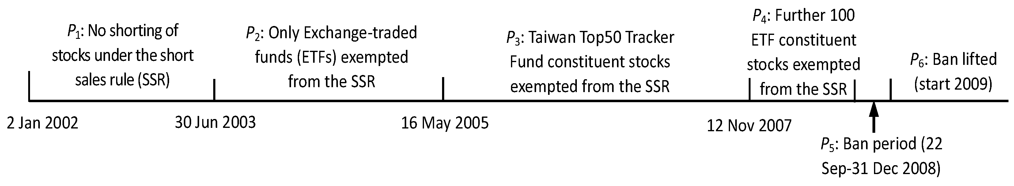
Figure 2.
Time plot for index prices, index returns, and price deviations, 2002-2009. This figure illustrates the time plot for the index price, the index returns, and the price deviations between 2002 and 2009, during which there are a total of six SSC policy changes (indicated by the vertical red lines): 2a presents the time plot for the index price and the equilibrium price; 2b presents the time plot for index returns; and 2c presents the time plot for deviations from the theoretical price.
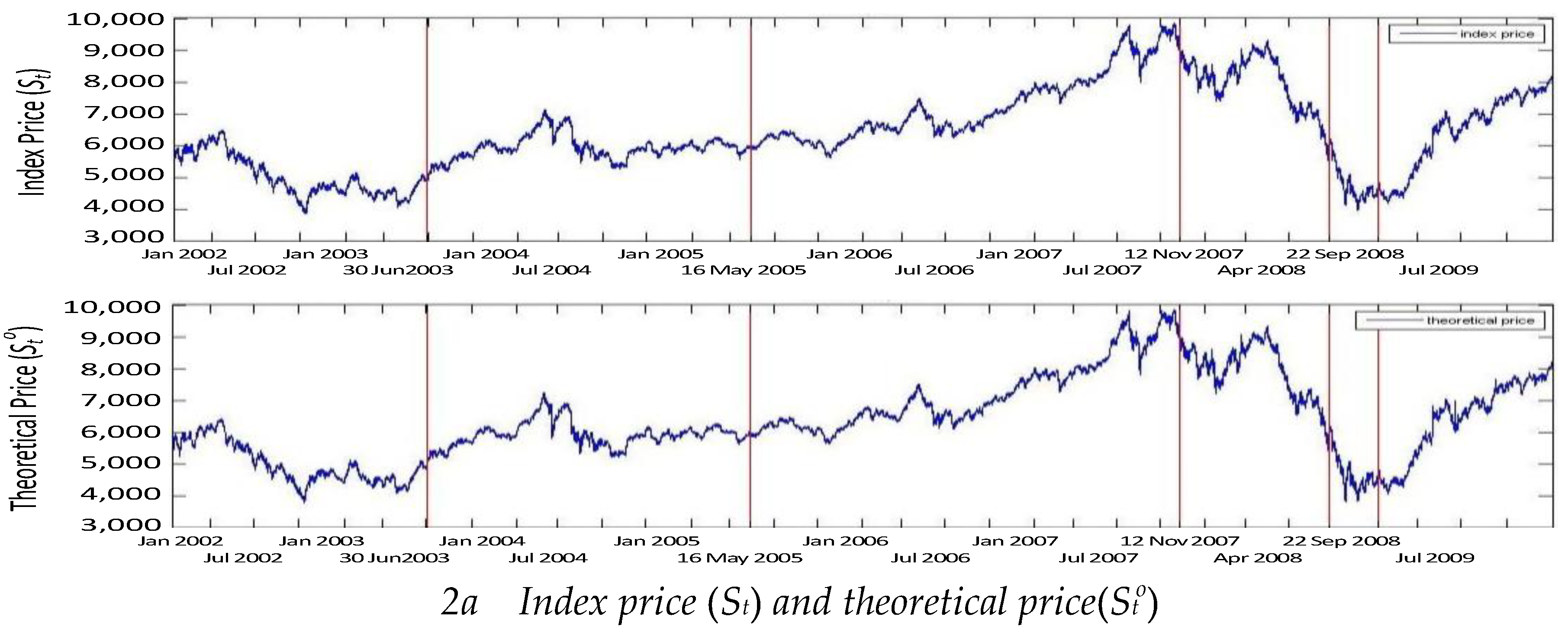
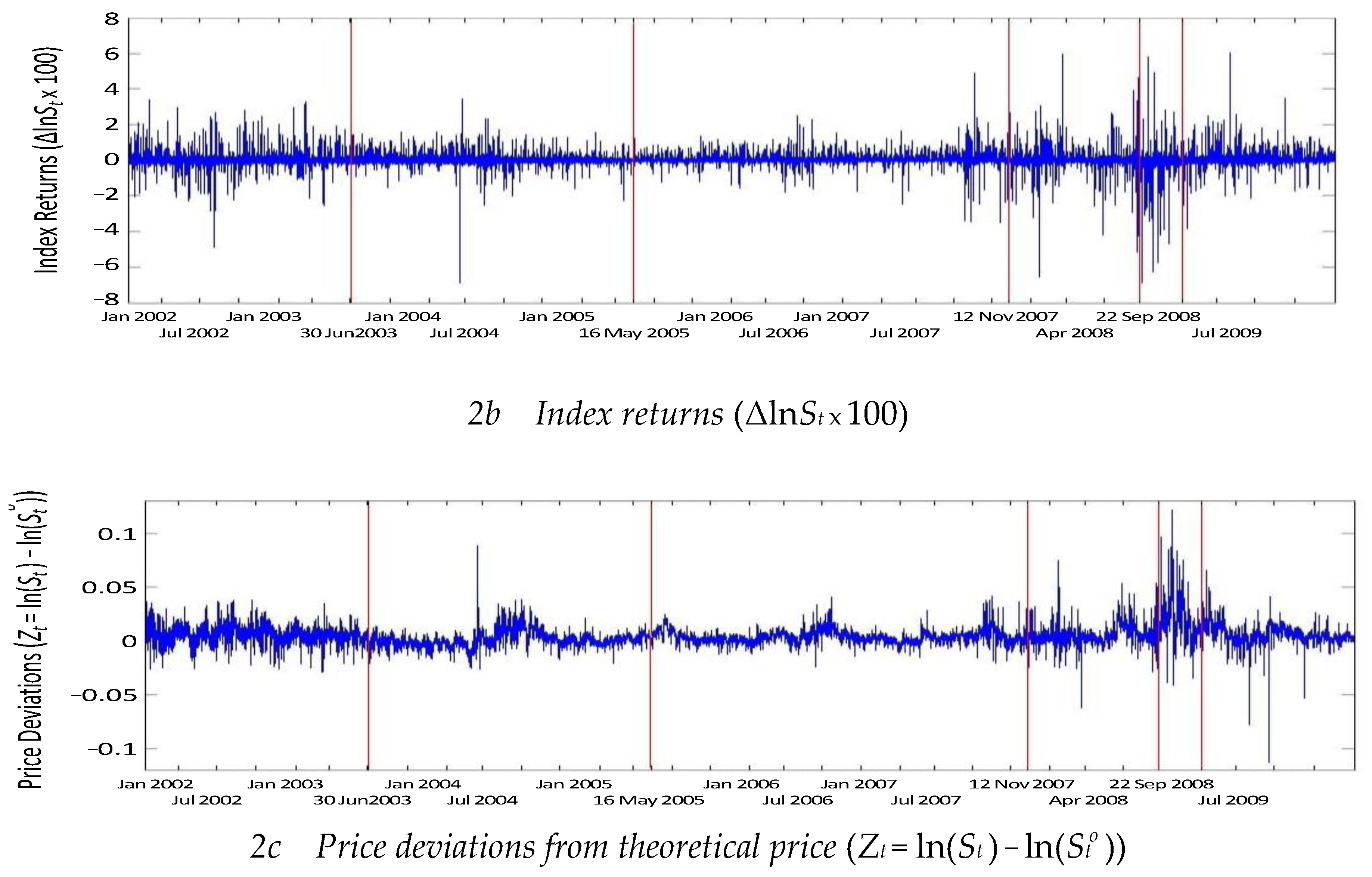
Figure 3.
Time Plot and Distribution of price deviations and index returns.Figure 3a presents the time plot for price deviations under different SSC pressures; Figure 3b concentrates on the tail behavior of the price deviations, and Figure 3c concentrates on the tail behavior of the index returns.
Figure 4.
Price difference from counterfactual analysis with/without short-sales ban. This figure shows the difference between the index price with and without the short-sales ban obtained from the counterfactual analysis. We assume that only the index price will change in cases where there is no short-sales ban. The blue (green) line denotes the price difference between the market index price with the short-sales ban and the mean (median) of the simulated market price without the short-sales ban. The first and second pairs of dashed lines indicate the start and end dates of the total bans on the short selling of all stocks.
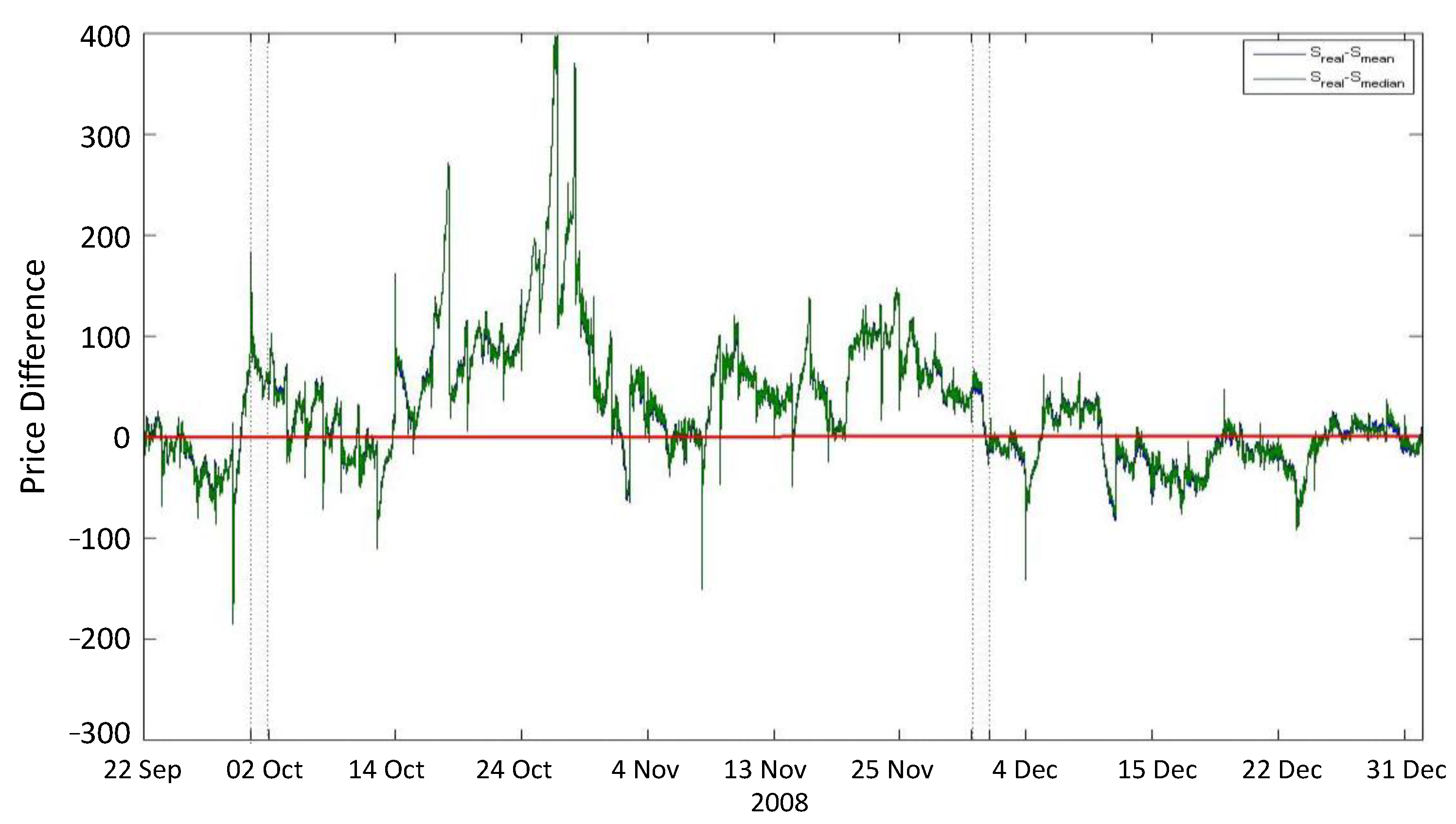

Table 1.
Unit-root and cointegration testsa.
| Measures | Statistics | Critical Values | First Difference | |
| t-Statistic | Critical Values | |||
| Panel A: Augmented Dickey-Fuller Test Statisticsb | ||||
| –1.38 | –3.43019 | –212.365 | –2.86136 | |
| –1.60 | –2.86136 | –287.005 | –2.86136 | |
| Panel B: Cointegration Testc | ||||
| Trace Test | 1180.2 | 25.87211 | – | – |
| Max-eigenvalue Test | 1176.0 | 19.38704 | – | – |
Notes:The sample period runs from Jan 2, 2002, to Dec 31, 2009, providing 1,989 trading days and 539,109 pairs of intraday observations. b lnSt denotes the logarithm of the TAIEX index price, refers to the logarithm of the one-minute theoretical price derived from put-call parity, both available from the Taiwan Economic Journal (TEJ) Database. c The cointegrating vector (the mispricing error or error correction term) as defined in Equation (2), which is estimated as (1, –0.99), is simplified to (1, –1).
Table 2.
Summary statistics.
| Variables | Full Sample | Sub-period Mean Values | |||||||||||
| Median | S.E. | Min | Max | Mean | |||||||||
| 6212 | 1307 | 3846 | 6421 | 9860 | 5024 | 5931 | 7239 | 8006 | 4790 | 6463 | |||
| 6174 | 1308 | 3774 | 6393 | 9848 | 4995 | 5922 | 7211 | 7963 | 4705 | 6428 | |||
| 0.0000 | 82 | –6905 | 0.0721 | 6047 | –0.1304 | 0.1612 | 0.2412 | –0.7021 | –1.3651 | 0.8505 | |||
| 0.0000 | 107 | –12810 | 0.0731 | 12744 | –0.1310 | 0.1673 | 0.2400 | –0.7111 | –1.4137 | 0.8723 | |||
| 0.0036 | 0.0074 | –0.1132 | 0.0047 | 0.1218 | 0.0058 | 0.0016 | 0.0039 | 0.0056 | 0.0183 | 0.0058 | |||
| No. of Obs. | 539,019 | 99186 | 126557 | 168020 | 57994 | 19241 | 68021 | ||||||
| Market liquidity | |||||||||||||
| Num_Trades | 2289 | 2807 | 0 | 152241 | 2862 | 2434 | 2467 | 2745 | 3507 | 2690 | 4011 | ||
| Num_Shares | 11477 | 17737 | 0 | 1063416 | 14877 | 12965 | 14971 | 14411 | 16936 | 12759 | 17485 | ||
| TDollart –1 | 281 | 434 | 0 | 35933 | 368 | 301 | 332 | 394 | 450 | 223 | 438 | ||
| Daily_Turnover | 0.0061 | 0.0030 | 0.0020 | 0.0223 | 0.0069 | 0.0082 | 0.0078 | 0.0059 | 0.0057 | 0.0048 | 0.0075 | ||
| Daily_Turnover/MV | 0.0062 | 0.0025 | 0.0021 | 0.0193 | 0.0068 | 0.0083 | 0.0070 | 0.0061 | 0.0061 | 0.0050 | 0.0074 | ||
| No. of Obs. | 1,989 | 366 | 467 | 620 | 214 | 71 | 251 | ||||||
| Market condition | |||||||||||||
| Realized_Variance*100 | 0.0101 | 0.0358 | 0.0009 | 0.4814 | 0.0186 | 0.0240 | 0.0158 | 0.0080 | 0.0272 | 0.0757 | 0.0188 | ||
| 0.0005 | 0.0021 | –0.0070 | 0.0060 | 0.0003 | 0.0001 | 0.0006 | 0.0008 | –0.0012 | –0.0053 | 0.0014 | |||
| 0.0148 | 0.0053 | 0.0068 | 0.0270 | 0.0148 | 0.0181 | 0.0127 | 0.0100 | 0.0200 | 0.0242 | 0.0187 | |||
| –0.1374 | 0.6337 | –1.9077 | 2.2563 | –0.1706 | 0.1864 | –0.1878 | -0.4167 | 0.1668 | 0.3709 | –0.4920 | |||
| 0.8466 | 2.4404 | –0.3963 | 16.2872 | 1.7216 | 0.3252 | 1.4754 | 2.4858 | 2.4188 | 0.2950 | 2.1374 | |||
Note: St (Sto) is the index (theoretical index) price; ΔlnSt (ΔlnSto) are the index (theoretical index) returns; Zt = ΔlnSt – ΔlnSto are the violations (deviations) from the difference of logarithmic index price. Three control variables include market liquidity, market condition and the microstructure effect. Num_Trades is the number of trades per minute; Num_Shares (x 1,000) is the number of shares traded per minute; TDollart–1 (x 1,000) is the amount of trading dollars per minute; Daily_Turnover is calculated as the daily trading volume divided by the daily number of outstanding shares; Daily_Turnover/MV is the daily trading dollars divided by the daily market value of the index. Realized_Variance is calculated by the daily one-minute index returns; and are the respective average returns, skewness, kurtosis, and standard deviations calculated by the previous 90-day one-minute return; NRt refers to the daily number of extreme negative index returns (extreme negative index returns are denoted as less than two standard deviations from the mean index return). We follow Fung and Jiang (1999) and Jiang et al. (2001) to measure market direction by the ‘relative strength index (RSI), with all observations being sorted into ten deciles based upon the daily RSI and the highest deciles representing the most extreme price movements, periods when short selling is more likely. The RSI is expressed as, where N t+ (N t– ) indicates the number of one-minute intervals of advances (declines) in the TWSE spot index during the day. The distribution of the index price, returns, price deviations, and control variables were also illustrated in Figure 2a. The average price deviation () in Equation (2) is more significant than zero and the patterns of the price deviations are asymmetric for each period, particularly during periods of strict constraints (as illustrated earlier in Figure 3a and 3b).
Table 3.
Three-regime TECM estimates under different policy changes.
| Models | (1)(i)b | (1)(ii)b | (2)(i)b | (2)(ii)b | ||||||||||||||||
| Variables | ΔlnSt | ΔlnSto | ΔlnSt | ΔlnSto | ΔlnSt | ΔlnSto | ΔlnSt | ΔlnSto | ||||||||||||
| Intercept | –0.0000 | 0.0000 | –0.0000 | † | 0.0000 | –0.0000 | † | –0.0000 | –0.0000 | † | –0.0000 | |||||||||
| αj+ | –0.0011 | † | 0.0012 | † | –0.0016 | † | 0.0014 | † | – | – | – | – | ||||||||
| αjbtw | –0.0007 | –0.0021 | † | –0.0017 | † | –0.0014 | – | – | – | – | ||||||||||
| αj– | –0.0100 | † | 0.0094 | † | –0.0105 | † | 0.0097 | † | – | – | – | – | ||||||||
| – | – | – | – | 0.0041 | † | 0.0070 | † | 0.0041 | † | 0.0073 | † | |||||||||
| – | – | – | – | –0.0055 | 0.0511 | † | –0.0049 | 0.0505 | † | |||||||||||
| – | – | – | – | –0.0002 | 0.0020 | † | –0.0012 | 0.0021 | † | |||||||||||
| – | – | – | – | –0.0143 | † | –0.0001 | –0.0157 | † | 0.0001 | |||||||||||
| – | – | – | – | 0.0008 | 0.0009 | 0.0001 | 0.0007 | |||||||||||||
| – | – | – | – | –0.0401 | † | –0.0038 | –0.0437 | † | –0.0033 | |||||||||||
| – | – | – | – | –0.0051 | † | 0.0008 | –0.0050 | † | 0.0009 | |||||||||||
| – | – | – | – | –0.2013 | † | –0.0152 | –0.2020 | † | –0.0151 | |||||||||||
| – | – | – | – | –0.0018 | † | –0.0008 | –0.0018 | † | –0.0006 | |||||||||||
| – | – | – | – | –0.0743 | † | –0.0022 | –0.0742 | † | –0.0025 | |||||||||||
| – | – | – | – | 0.0009 | 0.0017 | 0.0002 | 0.0019 | |||||||||||||
| – | – | – | – | 0.0009 | 0.0123 | † | –0.0009 | 0.0124 | † | |||||||||||
| – | – | – | – | 0.0009 | –0.0052 | 0.0011 | –0.0043 | |||||||||||||
| – | – | – | – | –0.0136 | –0.0045 | –0.0148 | –0.0051 | |||||||||||||
| – | – | – | – | 0.0014 | 0.0748 | –0.0001 | 0.0732 | |||||||||||||
| – | – | – | – | 0.0017 | –0.0013 | 0.0023 | –0.0005 | |||||||||||||
| – | – | – | – | 0.0009 | –0.0009 | 0.0008 | –0.0002 | |||||||||||||
| – | – | – | – | –0.0007 | 0.0971 | –0.0335 | 0.0811 | |||||||||||||
| TDollart–1 | – | – | –0.0000 | † | 0.0000 | – | – | –0.0000 | 0.0000 | |||||||||||
| – | – | –0.0006 | 0.0015 | – | – | 0.0008 | 0.0010 | |||||||||||||
| – | – | –0.0000 | † | 0.0000 | – | – | –0.0000 | † | –0.0000 | |||||||||||
| – | – | 0.0014 | † | –0.0004 | – | – | 0.0009 | –0.0002 | ||||||||||||
| – | – | 0.0000 | –0.0000 | – | – | 0.0000 | 0.0000 | |||||||||||||
| Overnight | – | – | 0.0002 | † | 0.0006 | † | – | – | 0.0002 | † | 0.0006 | † | ||||||||
| Open | – | – | 0.0001 | † | 0.0000 | † | – | – | 0.0001 | † | –0.0000 | † | ||||||||
| Close | – | – | –0.0000 | 0.0000 | – | – | –0.0000 | 0.0000 | ||||||||||||
| AIC | –22.6123 | – | –22.6152 | – | –22.6218 | – | –22.6249 | – | ||||||||||||
| –0.0089*** – | –0.0089*** – | – | – | – | – | |||||||||||||||
| – | – | – | –0.0033*** – | –0.0032*** – | ||||||||||||||||
Notes: The Model (1) and (2) estimates are specified in Equations (3) and (4). () refers to the speed of downward (upward) adjustments, accounting for all transaction costs (such as ); refers to the speed of the adjustment in the interband while the other notations follow the same previous definitions. () is the downward (upward) adjustment speed, taking all transaction costs into account under the various policy changes ( and ). H01a (α S– – α S+ ≥ 0) tests whether there is an asymmetric pattern in the speed of upward vs. downward adjustment, and H01b (α S+ , P4 – α S+ , P5 ≥ 0) tests whether the speed of downward adjustment improves under strict SSCs; other notations are the same as in the notes to Table 2. The TECM threshold values are provided in Section 4.1. *** denotes significance at the 1% level. † significantly differs from zero if its conventional t value is greater than the sample size-adjusted critical t value, 3.65. The value is calculated by Connolly (1989) who illustrated that the conventional t value criterion is not appropriate if the sample size is large.
Table 4.
SSCs policies versus return distribution characteristicsa.
| Periods | No. of Obs. | Skew | Kurt | Extre. Freq– | Extre. Freq+ | *100 | *100 |
| 366 | 0.9126 | 56.04 | 0.0054 | 0.0063 | 0.0240 | 0.0106 | |
| 467 | 0.8683 | 32.62 | 0.0092 | 0.0111 | 0.0158 | 0.0079 | |
| 620 | 2.6429 | 75.12 | 0.0049 | 0.0058 | 0.0080 | 0.0034 | |
| 214 | 1.0573 | 96.01 | 0.0031 | 0.0037 | 0.0272 | 0.0141 | |
| 71 | –3.0075 | 120.54 | 0.0032 | 0.0034 | 0.0757 | 0.0530 | |
| 251 | 2.8151 | 75.75 | 0.0073 | 0.0071 | 0.0188 | 0.0064 | |
| p4 − p5b | 4.0648*** | –24.54*** | –0.0003 | 0.0003 | –0.0484*** | –0.0389*** | |
Notes: a The measures, Skew and Kurt represent the daily skewness and excess kurtosis of the index returns; Extre.Freq– (Extre.Freq+) refers to the magnitude of the daily occurrences of extreme negative (positive) returns, which are defined as index returns that are less than (greater than) twice the standard deviation for each policy change period. Realized_ Variance is the sum of the squared daily one-minute index returns. Downside_Risk represents realized semi-variance, that is, the sum of squared negative returns. b *** denotes significance at the 1% level with the Newey-West standard errors.
Table 5.
TECM estimates with ‘high propensity to short’ (HPTS).
| MODEL | (3) | (4) | (5) | (6) | |||||||
| Dep. Var. | |||||||||||
| Intercept | -0.0000 | 0.0000 | Intercept | -0.0000 | 0.0000 | Intercept | -0.0000 | 0.0000 | Intercept | -0.0000 | -0.0000 |
| -0.0055† | 0.0011 | -0.0035† | -0.0004 | -0.0026 | 0.0055† | -0.0032† | 0.0026 | ||||
| -0.0262† | 0.0174† | -0.0023 | -0.0009 | 0.0129† | 0.0495† | ||||||
| -0.0051† | -0.0025 | -0.0028 | -0.0025 | ||||||||
| -0.0083† | -0.0002 | 0.0007 | 0.0042 | ||||||||
| -0.0038† | 0.0028 | -0.0035† | -0.0029 | ||||||||
| -0.0148† | 0.0059 | -0.0573† | 0.0060 | ||||||||
| -0.0050† | -0.0007 | ||||||||||
| -0.3309† | 0.0228 | ||||||||||
| -0.0010 | 0.0025 | ||||||||||
| -0.2231† | 0.0016 | ||||||||||
| -0.0051 | -0.0042 | ||||||||||
| -0.0326† | 0.0241† | ||||||||||
| -0.0028† | 0.0028† | -0.0025† | 0.0026† | -0.0027† | 0.0029† | -0.0024† | 0.0026† | ||||
| -0.0000† | 0.0000 | -0.0000† | 0.0000 | -0.0000† | 0.0000 | -0.0000† | 0.0000 | ||||
| -0.0007 | 0.0028 | -0.0005 | 0.0027 | -0.0007 | 0.0028 | 0.0003 | 0.0029 | ||||
| 0.0017† | -0.0009 | 0.0015† | -0.0008 | 0.0016† | -0.0011 | 0.0012† | -0.0007 | ||||
| -0.0000† | -0.0000 | -0.0000† | -0.0000 | -0.0000† | -0.0000 | -0.0000† | -0.0000 | ||||
| -0.0000 | 0.0000 | -0.0000 | 0.0000 | -0.0000 | 0.0000 | -0.0000 | 0.0000 | ||||
| overnight | 0.0001† | 0.0006† | 0.0002† | 0.0006† | 0.0001† | 0.0006† | 0.0002† | 0.0006† | |||
| open | 0.0001† | -0.0000† | 0.0001† | -0.0000† | 0.0001† | -0.0000† | 0.0001† | -0.0000† | |||
| close | -0.0000 | 0.0000 | -0.0000 | 0.0000 | -0.0000 | 0.0000 | -0.0000 | 0.0000 | |||
| AIC | -22.6144 | -22.6151 | -22.6146 | -22.6202 | |||||||
| Asymmetry Test | |||||||||||
| -0.0226*** | |||||||||||
| Different Policy Test | |||||||||||
| -0.0045*** | |||||||||||
| Downward Adjustment Test | |||||||||||
| -0.0039*** | |||||||||||
Note: The equations of Models (3-5) are provided upon request, and Model (6) estimates are specified in Equation (8). The highest RSI deciles are denoted as ‘high propensity to short’ (HPTS) or transactions with high short demand. The observations are sorted into ten deciles based upon the daily ‘relative strength index’ (RSI), with the highest deciles representing the most extreme downward price movements, periods when short selling is more likely. The RSI is expressed as: , where N t+(N t– ) indicates the number of one-minute intervals of advances (declines) in the TWSE spot index during the day. αjk denotes the speed of adjustment in cases of ‘high propensity to short’ (HPTS) under different conditions of k, such as j= S or SO. *** indicates significance at the 1% level with the Newey-West standard errors. † significantly differs from zero if its conventional t value is greater than the sample size-adjusted critical t value of 3.65. The value is calculated by Connolly (1989), who illustrates that the conventional t-value criterion is not appropriate if the sample size is large.
Table 6.
Regression Identification of Elevated Risk Due to Tighter SSC Policya.
| Dependent Variable | No. of Obs. | Interceptb | b | b | VIXb | |||||
| Realized_Variance*100 | 768 | –0.0343 | * | 0.0011 | 0.0162 | ** | –0.0111 | * | 0.0020 | * |
| Downside_Risk*100 | 768 | –0.0182 | * | 0.0000 | 0.0220 | * | –0.0091 | * | 0.0011 | * |
Notes:a The table reports the results that specifically regress the and on a set of dummy variables characterizing different SSC regimes and the TAIEX VIX. The Realized_Variance variable is the sum of the squared daily one-minute index returns; the Downside_Risk variable refers to daily realized semi-variance (that is, the sum of the squared negative returns); and VIX is the hybrid proxy for the market-wide investor sentiment and volatility. P3, P5, and P6 are dummy variables representing the different regimes from 2008 to 2009. b * denotes significance at the 10% level, ** at the 5% level, and *** at the 1% level with the Newey-West standard errors.
Disclaimer/Publisher’s Note: The statements, opinions and data contained in all publications are solely those of the individual author(s) and contributor(s) and not of MDPI and/or the editor(s). MDPI and/or the editor(s) disclaim responsibility for any injury to people or property resulting from any ideas, methods, instructions or products referred to in the content. |
© 2025 by the authors. Licensee MDPI, Basel, Switzerland. This article is an open access article distributed under the terms and conditions of the Creative Commons Attribution (CC BY) license (http://creativecommons.org/licenses/by/4.0/).
Copyright: This open access article is published under a Creative Commons CC BY 4.0 license, which permit the free download, distribution, and reuse, provided that the author and preprint are cited in any reuse.


