
Submitted:
28 July 2025
Posted:
29 July 2025
You are already at the latest version
Abstract
This paper presents two distinct but related empirical analyses of the Irish Day-Ahead electricity market, which underwent a structural change during the study horizon due to a Brexit-related shift in market coupling. First, we examine the activity of speculators (i.e. financial traders), measuring their overall market share in terms of order volumes and executed trades. We also assess the proportion of trading periods in which speculators are marginal, that is when their bid or offer prices equal the market-clearing price. Despite their relatively small share of total market activity, we find that speculators are marginal in a significant percentage of trading periods. We also identify a clear shift in their behavioural patterns following the structural market change. The second analysis introduces an intuitive method to quantify price inertia, the extent to which market prices resist small changes in demand or supply. While conceptually similar to liquidity or order book depth in continuous trading environments, this approach is applied within the context of a Day-Ahead auction market. We observe that price inertia levels also change following the structural shift. The Irish market offers a representative and transparent setting for short-term European electricity markets, allowing for clear identification of participant types. A clearer understanding of both aspects is essential for regulators evaluating market design as well as for market participants managing risk in Day-Ahead markets.
Keywords:
electricity markets
; day-ahead market
; bid and ask curves
; price inertia
; speculators
1. Introduction
Electricity markets have become a prominent area of academic research in recent decades driven by transformative developments such as market deregulation, the rapid expansion of renewable generation and the growing availability of short-term trading opportunities. These changes have spurred research across diverse areas including market power and competition [1,2], price volatility [3], electricity price forecasting [4,5,6,7], portfolio and asset optimisation [8], and market dynamics [9]. In many jurisdictions the Day-Ahead (DA) market is one of the main routes to market through which electricity participants hedge or rebalance their positions ahead of physical delivery. DA market prices serve as reference prices for a range of financial derivative contracts and also influence retail electricity pricing. Given its central role, further insights into the functioning of DA markets remain important. This paper contributes to that effort by examining two distinct but interrelated topics within a DA market setting: the activity of financial traders and price inertia, the latter defined as the extent to which market prices resist small shifts in demand or supply. A deeper understanding of these aspects is relevant for regulators evaluating market design and liquidity, as well as for participants active in short-term electricity markets.
As noted by [10], the role of financial traders in commodity and energy markets has been examined in a range of studies. In the context of short-term electricity markets, we refer to financial traders as speculators, defined as participants that neither generate nor consume electricity but instead earn profits or incur losses based on the spread between their buy and sell prices either within the same market or across different market timeframes. In several U.S. electricity markets speculators can engage in Virtual Bidding, a mechanism that enables them to profit from the spread between DA and Real-Time (RT) prices1. This topic has been examined in studies such as Parsons et al. [2015], which presents cases where Virtual Bidding narrows the DA–RT spread but offers limited system benefits. In contrast, [14] find that Virtual Bidding can enhance liquidity and transparency, reporting a reduction in both the spread and its volatility in California’s wholesale market. In [15] it is seen that lower transaction costs in MISO were accompanied by increased speculator participation, altered generator behaviour, and improved consumer welfare. Meanwhile, Birge et al. [2018] observe that speculators may reduce forward premiums (i.e the DA-RT spread), although their impact is constrained by capital and regulatory limits2. While this U.S. focused literature offers valuable insights into price spreads and market efficiency, our study addresses a different and underexplored question: the presence and commercial behaviour of speculators in a European DA market. In contrast to the definitional ambiguity found in some of the broader commodity and energy market literature alluded to by [10], our analysis offers a clear and transparent framework for identifying speculators and quantifying their presence in a short-term European electricity market setting.
While prior research has examined short-term electricity market price volatility and the occurrence of price spikes, relatively little attention has been given to price inertia in these settings. Studies addressing volatility include, among others, [17,18,19,20]. In particular, [20] analyse demand and supply shocks in the Nordic market and show that price jumps are more likely when the system is operating near capacity constraints. In terms of price inertia in DA markets, studies such as [21] and [22] touch on the concept indirectly, as their methodologies examine the effect of larger supply shifts on prices. In a DA electricity price forecasting context, [23] present a single trading period example illustrating how steep supply or demand slopes can lead to high price sensitivity to external shocks, a similar intuition underlies our approach to measuring price inertia. One rare example of work that explicitly considers market stability is [24] which finds that increased integration and competition in the Nordic market led to more stable and less volatile prices. While conceptually related to our analysis, their approach differs methodologically and uses daily average prices, whereas we focus on hourly price data. In this paper, we propose an intuitive and easily understood method for quantifying price inertia in DA markets. Our approach draws conceptual inspiration from liquidity measures and depth analysis techniques commonly encountered in continuous trading markets, tools that are familiar to many practitioners, but is developed specifically for an auction-based setting.
1.1. Research Questions
This paper addresses two distinct but related research questions:
- What is the extent of speculator participation in the market, and how has it evolved over time?
- Can we define a clear and intuitive approach to measuring price inertia, and how has it changed over time?
To answer the first question, we use granular participant-level order and trade data to quantify the share of overall market activity attributable to speculators and to measure their influence on price setting, specifically how often their bids or offers equal the market-clearing price (i.e., marginality3). We also examine how speculator behaviour changed following a structural market change. To answer the second question, we introduce a sensitivity-based method for quantifying DA price inertia using publicly available hourly demand and supply curves, capturing how market prices respond to small shifts in supply or demand.
Our findings show that speculators are frequently marginal in the DA auction despite representing a small share of total market activity. We also observe a shift in price inertia following the structural market change.
This research contributes to the literature by providing additional insights into the functioning of DA electricity auctions. While the role of speculators in influencing price spreads has been studied extensively in U.S. short-term electricity markets, we are not aware of any empirical studies focusing specifically on speculators in European auction-based DA markets. This paper presents evidence that speculators are a significant presence in the market, particularly in terms of marginal pricing. Our second contribution is the development of an intuitive and transparent methodology for quantifying price inertia in DA markets. This is especially relevant in the context of ongoing market design and reform discussions, such as Great Britain’s Review of Electricity Market Arrangements [29,30]. Although price volatility has been well studied, its underlying drivers, such as low price inertia, remain comparatively underexplored ([24] presents a similar motivation in their work on market stability). Price inertia, as an additional market metric, can inform the evaluation of market design proposals by offering insight into how sensitive prices are to small shifts in demand or supply, an important consideration when evaluating past, present and potentially future price dynamics. The appeal of our approach lies in its conceptual clarity and ease of implementation. It offers a new analytical lens, similar in spirit to liquidity or order book depth analysis in continuous markets, but developed specifically for an auction-based setting. In addition to its practical applicability, our analysis provides concrete evidence on how DA price inertia evolved before and after a structural market change. While the methodology we propose is purposefully straightforward and transparent, it is informed by the complexity of the market environment, which makes an observational, data-driven approach both appropriate and necessary. These complexities, along with the key simplifying assumptions underlying our analysis, are discussed in subsequent sections.
1.2. Paper Structure
The structure of the remainder of the paper is as follows: in Section 2 we present both an overview of the Irish short-term electricity market and related pricing algorithms, we also provide a hypothetical example of a speculator in this setting. In Section 3 we detail the data sources and methodology. Section 4 presents the empirical analyses whilst in Section 5 we discuss the main findings. In Section 6 we conclude. Supplementary details and materials are available in the accompanying appendices.
2. Market Structure
2.1. Market
The Integrated Single Electricity Market (I-SEM), is the electricity market in Ireland. Although it is a small market (net electricity consumption in Ireland in 2021 was 30TWh, the equivalent figure for Great Britain was 305TWh [31]) it typifies spot European wholesale electricity market structures. The Irish electricity market is an example of what is called a multi-settlement electricity market, that is where the bidding and dispatch of electricity for a specific trading period is managed in successive runs. Some of the routes to market, that is how to buy and sell electrical energy, include
- Day-Ahead (DA) market: at 11am on day D participants submit orders to buy or sell electricity for hourly delivery periods in the [11pm D, 10pm D+1] interval. The market coupling algorithm, EUPHEMIA (Section 2.2), takes these inputs, in conjunction with interconnector transmission capacities (and other factors), and determines hourly prices and the direction of energy flow on the interconnectors. If the network is congested then zonal prices will diverge.
- Intraday (ID) market: after the DA auction has cleared additional auctions are held; these auctions, IDA1, IDA2 and IDA3 are similar in nature to the DA with the main differences being that they are held closer to the delivery time and the delivery periods are 30 minute intervals4.
- Intraday Continuous (IC) market: this is an important market in other European jurisdictions, but in an Irish electricity market context it comprises less than half a percent of traded energy volumes over the study timeframe and hence it is ignored here.
- Balancing (B) market: one hour prior to delivery ex-ante5 trading opportunities cease and the Transmission System Operator (TSO), takes over. The TSO compares forecast demand versus forecast generation, including what volumes have been traded in the ex-ante markets, and dispatches on/off units to ensure that supply meets demand. The prices that result from these dispatch decisions are called settlement imbalance prices (or Balancing market prices).
Securing a physical position in the Irish electricity market requires participation in one of the above markets. The market structure therefore provides a non-trivial level of (DA) liquidity. Again, for clarity purposes we note that speculators that are active in the Irish electricity market do not consume or generate electricity.
Structural Market Change
For the study timeframe the electricity markets in Ireland and Great Britain were connected via two interconnectors. Prior to Great Britain leaving the EU (i.e. Brexit), the these markets were coupled in DA and IDA1 auctions; post 1st January 2021 the coupling now takes place at the IDA1 and IDA2 auctions [32,33].
2.2. Pricing Algorithm
This section provides a brief description of the DA market pricing algorithm. It will be seen that the algorithm is more complex than a simple intersection of supply and demand curves and a complete description (including implementation details) is not publicly available. This combination of complexity and relatively limited transparency is one reason we adopt a reasonably straightforward observational approach when analysing speculator behaviour (Section 3.2). We also note that our price inertia analysis (Section 3.3) relies on a key simplifying assumption that abstracts from the full market-clearing process.
EUPHEMIA, the Pan-European Hybrid Electricity Market Integration Algorithm, is the algorithm used to calculate hourly DA market prices in a number of European markets. The EUPHEMIA Public Description [34] explains
- "The algorithm can handle a large variety of order types at the same time"; these include Aggregated Hourly Orders, Complex Orders (including Minimum Income Condition, MIC, and/or Load Gradient constraints), Scalable Complex Orders and Block Orders.
- The algorithm solves a Welfare Maximization Problem (Master Problem) and three interdependent sub-problems one of which is the Price Determination Sub-Problem. In the Master Problem "EUPHEMIA searches among the set of solutions for a good selection of block and MIC orders that maximises the social welfare. Once an integer solution has been found for this problem, EUPHEMIA moves on to determine the market clearing prices." i.e. the Price Determination Sub-Problem.
From the above, it is clear that viewing the algorithm solely as the intersection of bid and ask curves, while intuitive, oversimplifies its underlying mechanics. The algorithm has undergone and continues to undergo incremental change [35,36], making it a dynamic rather than static construct. In contrast to EUPHEMIA, for which only a high-level description is publicly available, the algorithm governing the Irish Balancing market for example is fully described in [37]6.
2.3. Speculators
We explain the concept of speculators in the Irish electricity market using a simple example. Consider a single speculator and delivery period. Suppose the speculator forecasts prices of €X/MWh in the DA/IDA1/IDA2/IDA3 ex-ante markets and forecasts a price of €(X+20)/MWh in the Balancing market. Based on these forecasts the speculator’s strategy is to buy in the cheaper ex-ante markets and implicitly sell in the more expensive balancing market (given that a speculator does not consume or generate electrical energy its balancing market position is simply the sum of its ex-ante positions for that trading period multiplied by a factor of ). If they buy 50MW/25MW/0MW/0MW in the DA/IDA1/IDA2/IDA3 markets, then their balancing market position will be a sell of 75MW. If the speculator’s forecasts are correct they stand to make a profit of €750 because the cost of the buys, €, is less than the income from the sell, €. Note the factor in the calculation is required because we are dealing with 30min intervals. If the forecast is incorrect then they could make more or less than €750, including a loss.
3. Materials and Methods
In this section we describe the underlying datasets and the empirical analyses. For context, we note that the data used in the study coincides with a diverse and volatile set of energy price regimes including the Covid-19 pandemic7 and the European energy crisis. Any reference to accompanying material in the appendices is for replicability and transparency purposes with the key details being captured in this Section 3.
3.1. Datasets
SEMOpx and SEMO are two of the bodies involved in the operation of the Irish electricity market [41,42]. Some of the datasets they publish include:
- Granular Participant Data: For each of the four ex-ante markets (Section 2.1) SEMOpx publishes a distinct file called the ETS Bid File. We use these files to interrogate the order and trade quantity data at a participant and trading period level of granularity. In each ETS Bid File positive (negative) order quantities represent purchase (sell) orders; the same convention applies to trade quantities. The DA ETS Bid file for example is published on a day+1 basis relative to the trading day and typically it consists of in excess of circa twenty thousand rows with an average of three hundred plus participants per auction.
- Bid Ask Curve Data: For each ex-ante auction SEMOpx publish a BidAskCurve file containing a monotonic increasing (decreasing) and anonymised view of the sell (buy) orders for each trading period in the auction8.
-
Other Data:
- –
- PUB_MnlyRegisteredCapacity files which provide participant registration data such as registered plant capacity and FuelType (if applicable).
- –
- PUB_30MinImbalCost file containing the Balancing Market price, , for trading period i. Similarly, MarketResult files containing DA, IDA1, IDA2 and IDA3 market prices (i.e. , , , and ).
In the Irish electricity market, participants may register one or more unit types, including Supply, Generator, Assetless, and Trading units, among others. These units have flexibility in their behaviour, so we follow the sequence of steps outlined in Appendix B to identify speculators.
3.2. Market and Speculator Analysis
Quantities
The DA market accounts for approximately 85% of the total volume traded across the DA, IDA1, IDA2, IDA3, and IDC markets. Therefore, we examine how DA volumes have evolved for speculators and for the market as a whole, with the latter providing context for the former. Using information in the DA market ETS Bid Files we derive a per trading period time series that shows
- The quantities of energy that participants were willing to buy or sell, we refer to these as the order quantities.
- The quantities of energy bought or sold which we term the matched quantities.
Marginal Participants
To understand which participants are marginal and whether or not this pattern has changed over time for each trading period (see Appendix D for details):
- We retrieve the bid and ask curves from the relevant BidAskCurve file and determine how they intersect.
- The intersection point(s) are then cross-referenced against the participant order data in the relevant ETS Bid File to determine which unit, or units, are marginal.
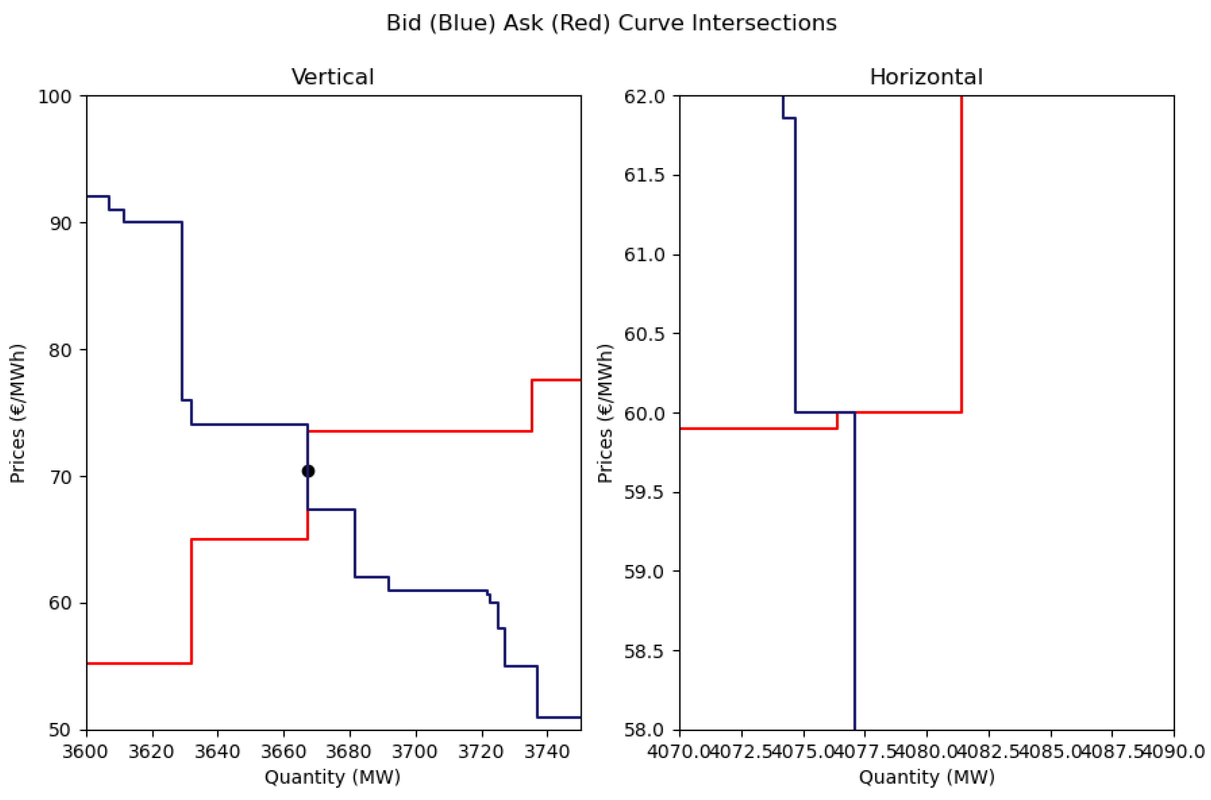
A by-product of the marginal analysis is the identification of bid and ask curve intersections. As a result, in addition to identifying marginal participants we also examine how DA bid and ask curves intersect and how these intersection patterns have evolved over time. Given the stepwise nature of the bid and ask curves in the Irish electricity market there are three possible types of intersection: horizontal (the curves are horizontally parallel and intersect over a ranges of quantities), vertical (the curves are vertically parallel and intersect over a ranges of prices) and perpendicular (the curves intersect perpendicularly at a single price and quantity point). For a perpendicular intersection, if at the point of intersection the ask curve is horizontal, ACH, we denote it as a perpendicular (ACH) intersection. Similarly, if at the point of intersection the bid curve is horizontal, BCH, we denote it as a perpendicular (BCH) intersection. In Appendix E we provide examples of different bid ask curve intersection types.
Aggregate speculator behaviour and profitability
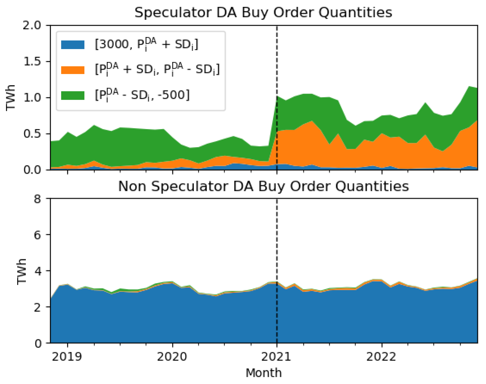
To understand how aggregate speculator behaviours have evolved over time we start by examining the speculator DA order (i.e. pre-market clearing) quantities referenced in Section 3.2.0.1. It is tempting to compare the speculator order quantity distributions (e.g. using kernel density estimates) at discrete points in time. However, here we take a less complicated approach yet still manage to capture the high level trends in a succinct manner. For trading period i, we denote the DA market price as and the the standard deviation of DA market prices for the corresponding hour over the previous 20 days as . We then partition the price domain into three distinct intervals defined as follows:
- Interval 1:
- Interval 2:
- Interval 3:
Here the and 3000 values correspond to the minimum and maximum permissible DA market prices9. For each price interval we calculate the sum of the speculator sell, and separately the speculator buy, order quantities that fall within that bucket. We then aggregate the values for each price interval by month and plot the monthly totals from November 2018 to December 2022.
Next, we consider the aggregate matched (i.e. cleared) speculator quantities. While we are primarily interested in the aggregate DA matched speculator quantities, motivated by the structural market change referenced in Section 2.1.0.1 and the hypothetical example in Section 2.3, we also examine the corresponding IDA1 and Balancing market values. With Speculator denoting the set of speculators participants and representing the quantity of power bought or sold (i.e. matched quantity) in trading period i by speculator j in market m we define
We calculate these variables for each trading period over the study horizon and present pair plots in order to identify any similarities or differences in aggregate speculator behaviours before and after the structural market change. For brevity we omit pair plots of the corresponding IDA2 and IDA3 Speculator values as these markets account for only a small share of ex-ante trading volumes. For clarity, similar to the hypothetical speculator example in Section 2.3, with , the values in equation 3 are obtained via
Finally, ignoring trading or transaction costs which in the Irish electricity market are minimal, our approach to estimating speculator profitability mimics the earlier hypothetical example. With , Speculator j’s profit and loss in trading period i is then estimated via
Here represents the market price for trading period i in market m. The factor in equation 5 reflects the buy and sell sign convention and 30 minute delivery periods. This calculation is then repeated for all speculator participants across all trading periods in the study horizon to produce an aggregate estimate of speculator profitability
3.3. Price Inertia Analysis
Our approach to measuring price inertia in the Irish DA electricity market involves applying a small horizontal shift to either the bid or ask curve and calculating the resulting intersection price. The difference between the market price and this new intersection price serves as a measure of price inertia. One could argue that obtaining the resulting intersection price would require a full rerun of the EUPHEMIA algorithm. However, since we apply only small horizontal shifts of 1 MW or 10 MW, minor relative to average forecast demand in the Irish DA market which was approximately 4300 MW per trading period over the study horizon, and the algorithm is not publicly accessible, we adopt a reasonable simplifying assumption: that a full rerun of the market pricing algorithm is not required. This approach is consistent with the existing literature where studies examining supply and demand curves in EUPHEMIA related contexts similarly rely on approximations or simplifications due to the unavailability of the algorithm. The process of applying a small horizontal shift of XMW (with X equating to 1MW or 10MW) to the DA ask curve in trading period i is as follows:
- Retrieve the bid and ask curve for trading period i from the relevant DA BidAskCurve file.
- Add the quantity X MW to each point on the ask curve
- Determine where this horizontally shifted ask curve intersects the bid curve. We call the resulting price the Simulated DA market price for trading period i, denoted by .
- With and as per Section 3.2.0.3, we define the Price Difference and Custom Metric values in trading period i as
If we consider the Price Difference time series that results from equation 6 on a stand-alone basis it is potentially misleading given the different commodity price regimes that existed over the study horizon (Figure A9 Appendix N presents a plot of the corresponding electricity market prices). Hence our interest in contextualising or normalising the Price Difference metric; we could do so by dividing by but this is undefined in trading periods in which the DA price is €0/MWh. Our approach is to instead divide by the standard deviation of market prices for that hour over the previous twenty days (i.e. ); other approaches are possible. We present the results of small horizontal shifts in the ask curves, results for small horizontal shifts in the bid curves are available but are omitted due to space constraints. Next, we briefly discuss two price inertia approaches that build on the above concepts and further enhance our intuition and understanding (we note however that in the following context the assumption of a small shift may not always hold true). The details are as follows.
Price Inertia Distribution
- For each trading period adjust the ask curve in MW increments until the simulated market price, , differs from the published market price. Let denote the shift required to observe the price change where the superscript indicates that we have used MW increments. Use equation 6 to calculate the associated price difference which we denote as .
- Repeat the previous step except use MW decrements to derive the corresponding and values.
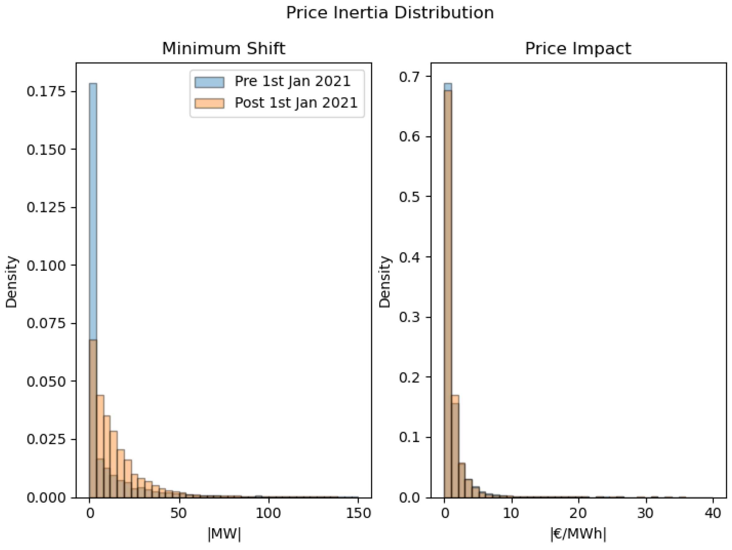
- For each trading period, define and calculate the Min Shift and Price Impact via
In Section 4.2 Figure 10 we present density histograms of the Min Shift and Price Impact values.
Order Example
This approach involves removing the order data for a single (speculator) participant, reconstructing the bid and ask curves using the remaining participants’ order data, and determining the new intersection price. Implementation details for this alternative approach and related examples are provided in Appendix L.
4. Results
4.1. Market and Speculator Analysis
Quantities
Figure 1 presents stacked area charts showing the sell order and sell matched quantities (Section 3.2.0.1) in TWh, grouped by FuelType10 and month for the Irish electricity market. The dashed vertical black line, also present in a number of subsequent plots, highlights the point in time at which the structural market change occurred (Section 2.1.0.1), recall the sign convention that sells (buys) are represented by negative (positive) quantities. It can be seen that approximately 52% of the sell order quantities will on average be matched. For conciseness, we do not present the corresponding buy plots, but it is worth noting that on average 83% of buy orders are matched. The presence of the Coal, Oil and Distillate categories in the sell order quantities plot and their absence for significant periods of time in the sell matched quantities plot is indicative of the Irish electricity market DA merit order.
A change in speculator sell order and sell matched quantities (i.e. red time series) post the structural market change is evident in Figure 1. From the underlying data it is seen that on average pre (post) the structural market change, speculators accounted for circa 10% (20%) of DA order quantities and approximately 2% (6%) of DA matched quantities. We note that while we identified 50 speculators in the Irish DA electricity market prior to the structural market change an average of 16 (14) speculators would submit sell (buy) orders to the DA whereas post the structural market change the corresponding number is 30 (24) speculators i.e. almost a doubling in the number of active speculators. For context we note that over the November 2018 to December 2022 timeframe there were 472 distinct participants in the Irish electricity DA market. Separately, it is interesting to note that for the IDA1 market which accounts for approximately 10% of traded volumes, speculators units have a significantly larger market share. On average speculators account for 54% (42%) of buy (sell) IDA1 order quantities and 46% (33%) of buy (sell) IDA1 matched quantities.
Marginal Participants
The top plot in Figure 2 presents a stacked area chart showing the percentage of marginal observations, grouped by fuel type and month. It can be seen that gas and multi-fuel units have exhibited a declining tendency to act as the marginal unit; prior to the structural market change this cohort was marginal in approximately 35% of trading periods compared to around 20% afterward. In contrast, speculator participants appear, at least visually, to be marginal in a greater proportion of trading periods post-change (rising from 49% before to 66% after). That speculators are marginal in the majority of trading periods stands in contrast to their overall minority presence in the market, as outlined in the previous paragraph.
The bottom plot in in Figure 2 presents a stacked area chart showing how the DA bid and ask curve intersections (i.e. vertical, horizontal or one of the two types of perpendicular intersection) have evolved since the market inception. A noticeable change occurs post the structural market change.
Aggregate Speculator behaviour and profitability
For insights into aggregate speculator pre market clearing behaviours we take summed DA speculator sell order quantity data from the top plot in Figure 1 (red time series) and split it by price interval (Section 3.2.0.3). Doing so, we arrive at the top plot in Figure 3. Again, to provide context, if we repeat the process but do it for non-speculators we obtain the bottom plot in Figure 3. For speculators it is clear that a lot of the increase in sell order quantities post the structural market change is associated with the price interval (orange time series). Examining the corresponding non-speculator data there is no obvious step change.
Plots of buy order quantity data, split by price interval for speculators and non-speculators, are provided in Appendix I, Figure A3. Similar patterns emerge from these plots, albeit there is a slight, visually imperceptible uptick in non-speculator buy order quantities within the price interval following the structural market change. Separately, we note that on average 97% of non-speculator buy order volumes occur in the interval which is an indication of the inelasticity of demand.
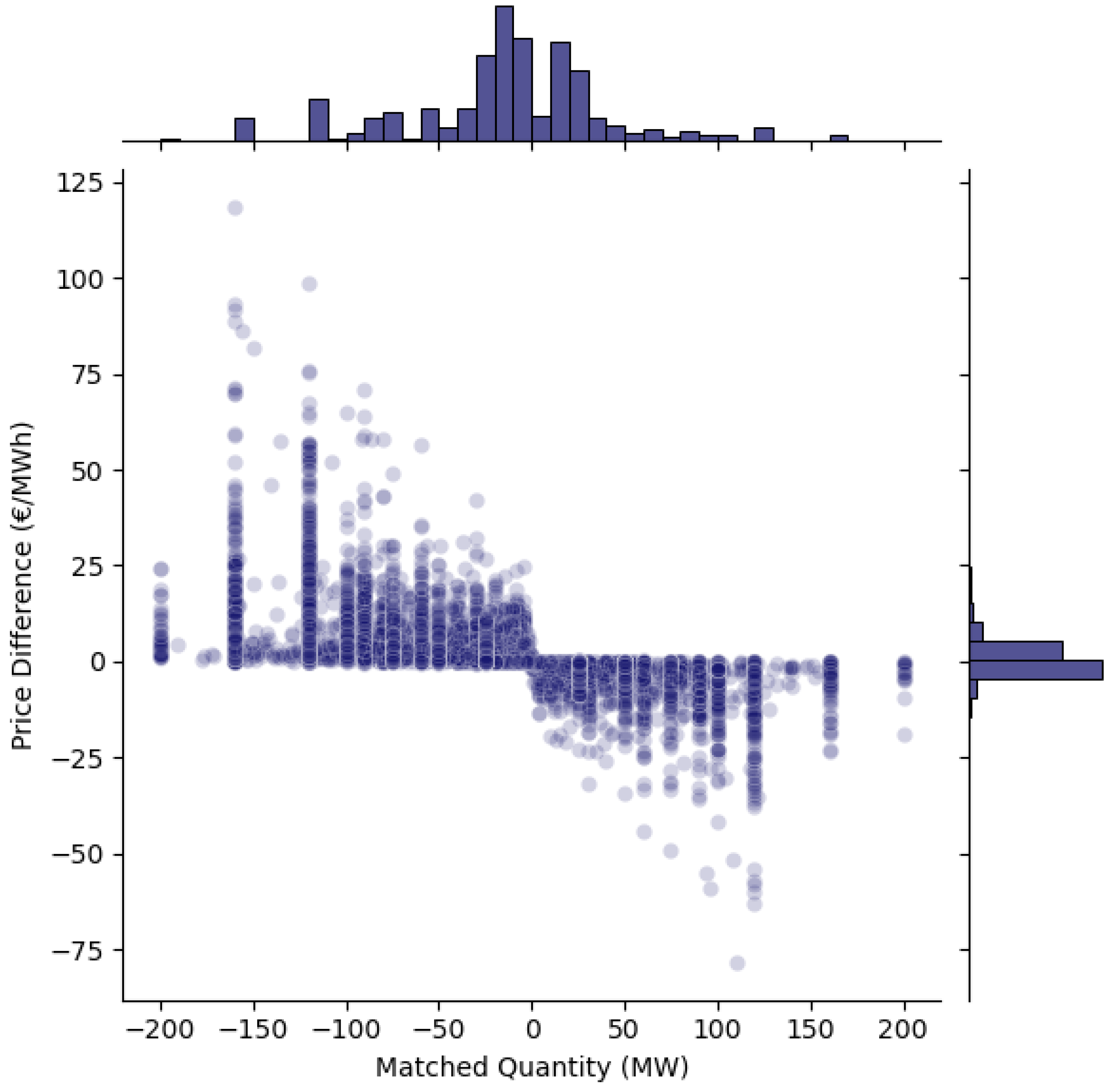
Figure 4 presents scatter plots of the Speculator IDA1 Matched Quantity (equation 2) against the corresponding Speculator DA Matched Quantity (equation 1) distinguishing between observations pre and post the structural market change. It is seen that post the structural market change the magnitude of speculator DA positions increased; a negative correlation between speculator positions in the DA and IDA1 markets is also clear (i.e. it is often the case that speculator DA matched quantities are partially or fully unwound in IDA1). In a similar manner Figure 5 plots the Speculator Balancing Market Quantity (equation 3) against the corresponding Speculator DA Matched Quantity, again we distinguish between observations pre and post the structural market change. It is seen that pre the structural market change there was a negative correlation between between the time series, but post the change the negative correlation is not apparent.
To provide some insight into aggregate speculator behaviour post January 2021 and also to highlight the general dynamism in their commercial behaviours, Figure 6 presents a granular time series view of two weeks worth of speculator data. The top plot in Figure 6 shows Speculator DA Matched Quantity in green and Speculator IDA1 Matched Quantity multiplied by a factor of in brown, the latter is denoted as Speculator IDA1 Matched Quantity (inverted). As per earlier comments, the visible correlation between the time series illustrates that speculator DA matched quantity positions are frequently, but not always, offset in the IDA1 market. The middle plot in Figure 6 shows Speculator Balancing Market Quantity values; given the preceding commentary (i.e. speculator DA positions are often partially or fully unwound in the IDA1) it is understandable that the magnitude of Speculator Balancing market quantities is less than the magnitude of corresponding speculator DA and IDA1 values. Taking the Speculator DA Matched Quantity time series in green from the top plot but splitting it into speculator buy matched quantities and speculator sell matched quantities, we arrive at the bottom plot. This plot highlights how speculators can have differing behaviours, that is speculators are not a homogeneous population. Moreover, this plot, and the other plots in Figure 6 once again illustrate the dynamic non-stationary commercial behaviours of speculators in the Irish electricity market.
Using equations 4 and 5, an estimate of the aggregate speculator profit and loss (P&L) from November 2018 to December 2022 is € million11. Of the total amount € million is attributable to calendar years 2021 and 2022. The six speculators referenced in Section 4.1.0.2 account for € million (i.e. 42% of estimated speculator profitability). Of the € million total, the amount that relates to speculators taking opposing positions in ex-ante markets (see Appendix G) is estimated at € million. Examining the granular P&L data (i.e. by speculator and trading period) then it can be seen that in circa 54% (46%) of observations in which there was a cash-flow it was positive (negative). This is indicative of the challenge speculators face in pursuing profitable trading strategies i.e. speculation in short-term electricity markets is not a risk-free activity.
4.2. Price Inertia Analysis
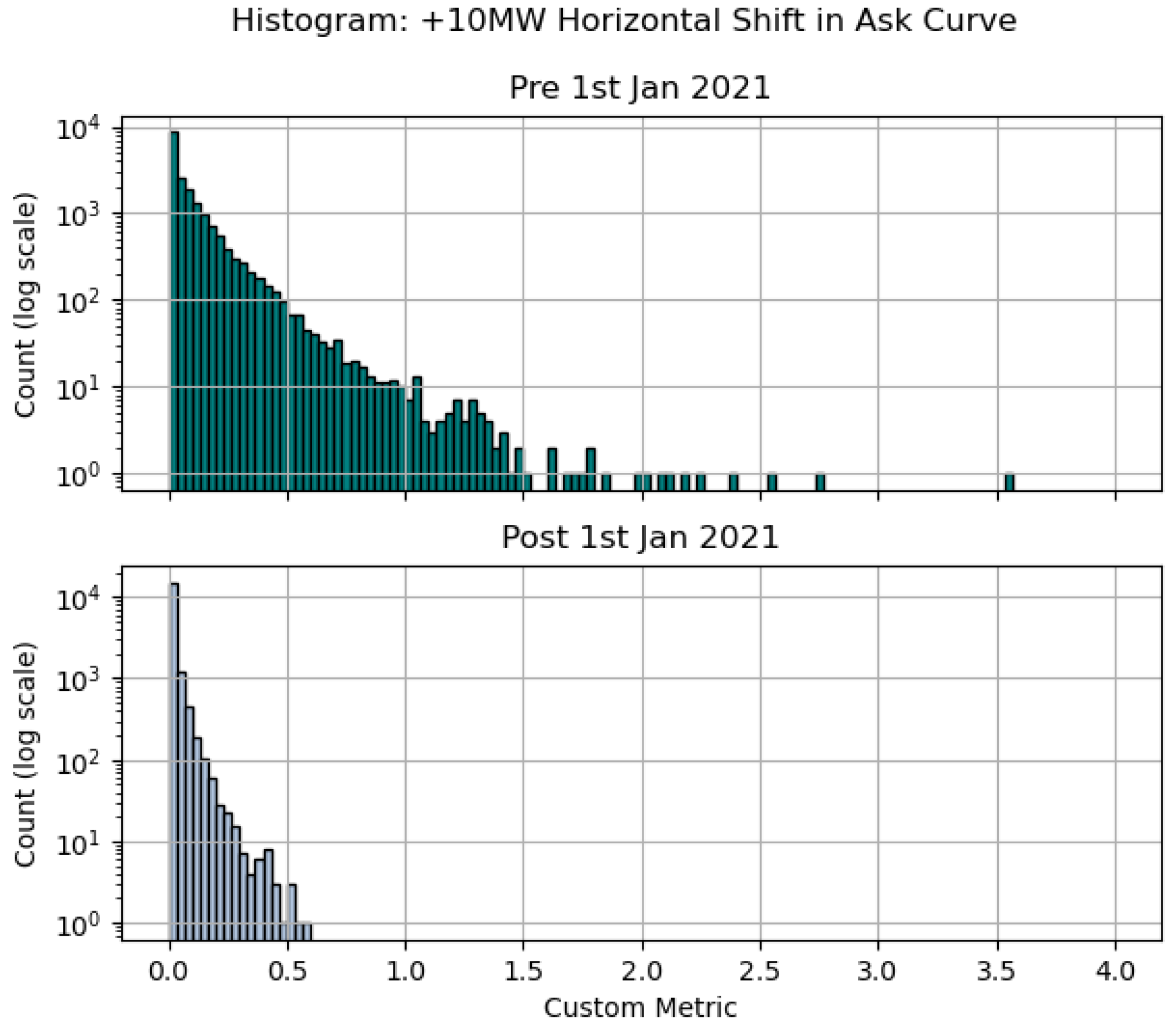
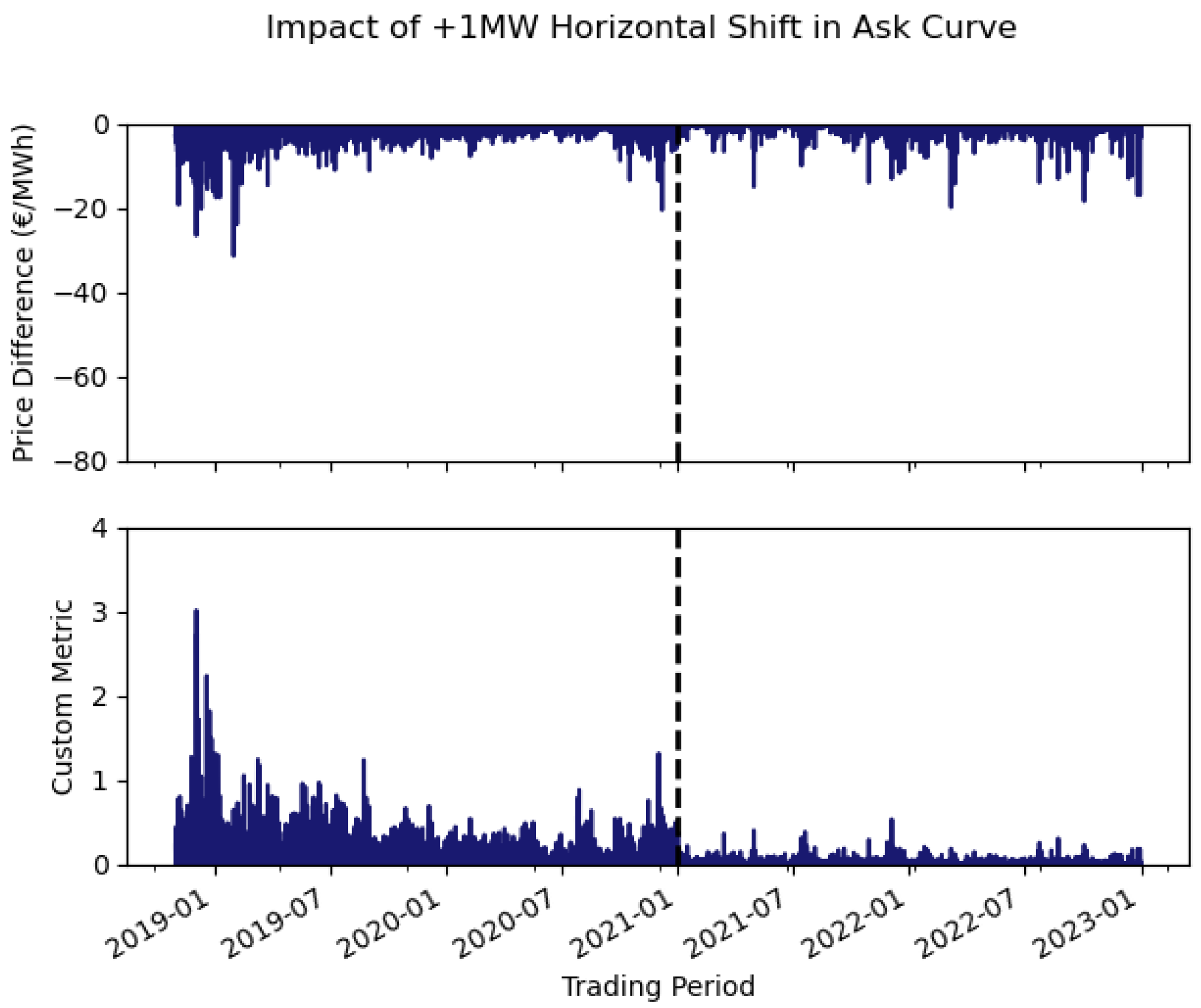
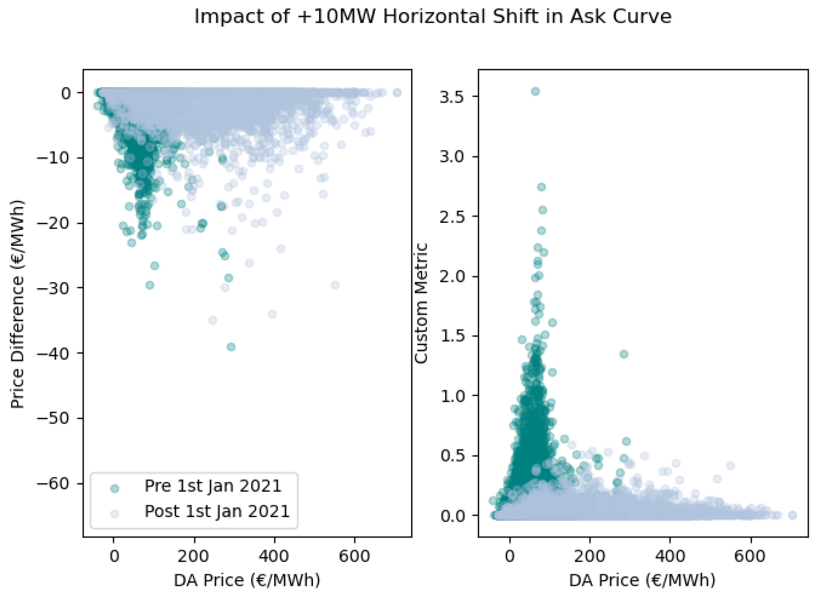
Taking bid ask curves from the November 2018 to December 2022 time frame, if we apply a +10MW horizontal shift to the ask curve and calculate the percentage of trading periods per day that have a Price Difference (equation 6) of €0/MWh, then we arrive at Figure 7. A step change in the percentage of zero price difference observations per day post the structural market change is visible. Using the time series values from the +10MW horizontal shift to the ask curve, the top plot in Figure 8 displays the Price Difference values per trading period while the bottom plot presents the corresponding Custom Metric values (equation 7). The Custom Metric plot shows a reduction in the horizontal shift impact from 2021 onwards. Examining the underlying data it is observed that in approximately 72% (36%) of all trading periods pre (post) 1st January 2021 the application of a +10MW horizontal shift would lead to a change in the market price. For those trading periods where the market price would change, it would lead to an average reduction of 3.6% (0.8%) in the DA price pre (post) 1st January 2021. We note in passing that, when comparing the proportion of trading periods with non-zero price differences before and after 1 January 2021, a two-proportion z-test rejects the null hypothesis that these proportions are the same12. In Figure 9 we take the Price Difference and Custom Metric time series values from Figure 8 and plot them against the corresponding DA price. From the scatter plots the difference in distributions pre and post the structural market change is evident. Note that in Appendix J Figure A4 and Figure A5 present histograms of the time series observations presented in Figure 8 while in Appendix K we present the corresponding +1MW price inertia analysis.
Figure 10 presents the price inertia distribution analysis described in Section 3.3. The density histogram on the left compares the distributions of the minimum shift required to trigger a market price change before and after 1 January 2021. It shows that, prior to this date, small shifts in the ask curve were more likely to result in a price change than comparable shifts after the change. Finally, in Appendix L we take a single speculator and simulate its impact on market prices. This approach is conceptually similar to the price inertia method although the assumption of a small shift in the demand or supply curve may not always hold.
Figure 10.
Price Inertia Distribution. Plot on the left is a histogram of the minimum absolute shift required to trigger a market price change (note: x-axis range restricted for display purposes), plot on the right is the estimated price impact.
Figure 10.
Price Inertia Distribution. Plot on the left is a histogram of the minimum absolute shift required to trigger a market price change (note: x-axis range restricted for display purposes), plot on the right is the estimated price impact.
5. Discussion
It is perhaps unsurprising that the Irish electricity market exhibits evidence of both the dynamism in aggregate speculator behaviours as well as a non-homogeneity in their behaviours. The empirical analysis also reveals that following the structural market change speculators participation in the DA market underwent a step change. In particular, their buy and sell order volumes within the price interval increased. At first glance, the frequency with which speculators were marginal, exceeding their overall market share both before and after the structural market change, may seem counterintuitive. However, on further reflection, this outcome is not entirely unexpected as the strategies employed by certain speculators involve placing a portion of their orders near the market-clearing price.
The price inertia analysis offered a straightforward and intuitive methodology. It was notable that the percentage of trading periods in which a small shift in the ask curve would have resulted in a market price change was relatively high and, in some cases, the resulting price changes were substantial. These findings highlight the susceptibility of DA electricity market prices to jumps or shocks, a characteristic feature with which many market participants will already be well versed. While our analysis focuses on the DA setting, the underlying concept is analogous to how participants often assess market depth and price sensitivity in other market environments. The shift in price inertia levels before and after the structural market change also stood out.
A plausible hypothesis linking the two preceding observations is as follows: after the structural market change, speculators began providing DA liquidity that had previously been supplied via EUPHEMIA’s interconnector scheduling between the Irish and British electricity markets. This behaviour aligns with one of the motivations for Virtual Bidding noted by [14] namely enhanced market liquidity and price transparency. A significant portion of this additional speculator liquidity appeared near the market-clearing price, potentially contributing to the observed increase in price inertia levels. While the correlation is suggestive, it does not establish causation. The ability to rigorously test this hypothesis is constrained by two key challenges:
- Pricing algorithm access: the market-clearing process is complex and only partially disclosed. Without full access to the EUPHEMIA algorithm, it is difficult to run counterfactual scenarios or isolate behavioural effects. We note [13] make related observations in their treatment of Virtual Bidding.
- Market dynamics: As noted by [15], market outcomes are shaped by evolving participant behaviours. Even subtle shifts in non-speculator actions either individually or in aggregate, for example the slight increase in non-speculator buy order volumes discussed in Section 4.1.0.3, could contribute to the observed changes.
Further research is warranted to explore this hypothesis more formally. One possible avenue is to forecast price inertia levels and identify the most influential explanatory variables, if indeed a model with meaningful predictive power can be developed. Even without additional research the empirical analysis hints at limitations in applying fundamental electricity price forecasting approaches to short-term markets. Speculators exhibit dynamic and adaptive behaviours, making the calibration of related input assumptions inherently challenging. Moreover, the price inertia analysis shows that small changes in supply or demand can, in certain trading periods, lead to material price movements, nonlinear effects that may be difficult to capture using fundamental models (or indeed many other modelling approaches).
6. Conclusions
In this paper we presented two distinct empirical analyses on the Irish electricity market. The study setting was representative of typical short-term European electricity markets with a structure that ensured a non-trivial degree of liquidity and the environment featured a high variable renewable generation penetration. The study period also coincided with a diverse range of commodity pricing regimes. The first piece of analysis examined the presence and strategic behaviour of speculators while the second addressed market price inertia. For speculators it was observed that the proportion of trading periods in which they were marginal was significantly in excess of their traded market share, they exhibited increased activity post a structural market change and the dynamism and non-homogeneity in their behaviours was also evident. The price inertia analysis introduced an intuitive and easily understood methodology and it also underlined the susceptibility or sensitivity of short-term electricity market prices to small changes in demand or supply. While an increase in the market price inertia levels post the structural market change was observed we could only conjecture as to the underlying causes given the domain complexity (i.e. the dimensionality of the repeated auction mechanism and lack of access to the market pricing algorithm). This research has two key implications. First, the findings on speculators and price inertia suggest inherent challenges in the ability of short-term fundamental market modelling approaches to accurately forecast electricity prices. Second, the price inertia methodology provides an additional metric that could be valuable when evaluating structural market change proposals. Our analysis contributes to the existing literature by reinforcing the understanding that short-term electricity markets are complex non-stationary environments with numerous interacting factors.
Author Contributions
Conceptualisation, J.C, A.A and K.M; methodology, J.C, A.A and K.M; data curation, J.C; investigation, J.C; writing - original draft, J.C; writing - review & editing, A.A and K.M; visualisation, J.C, A.A and K.M; supervision, A.A and K.M. All authors have read and agreed to the published version of the manuscript.
Funding
This research received no external funding.
Data Availability Statement
Use of Artificial Intelligence
During the preparation of this work, after completing a draft manuscript, the author(s) used ChatGPT and Gemini to refine and suggest alternative wording for certain sentences. Some suggestions were incorporated, others were not. All analysis and results presented in the manuscript are solely the author(s)’ own work. The author(s) take full responsibility for the content of the published article.
Conflicts of Interest
The authors declare no conflicts of interest. It is worth noting that while Joseph Collins reports a relationship with capSpire (a technology consulting and solutions company that specialises in the commodities/energy industry) that includes employment, the manuscript reflects the authors independent research.
Appendix A. Simplifications and Other Considerations
Some of the simplifications, considerations and caveats related to the analysis include
- As noted in Section 3.3 in the price inertia analysis we use the simplifying assumption that a small horizontal shift in either the ask or the bid curve does not require a rerun in the EUPHEMIA algorithm.
-
This alternative definition may be of interest for those trading periods in which the published bid and ask curve intersects vertically (Figure A2 Appendix E). Using this definition, while the percentages presented in Section 4.2 (and the graphs in Appendix K) will change, the overall pattern remains the same. That is, a step change in the impact of a small horizontal shift in the ask curve from January 2021 onwards is observed.
- We classify Irish electricity market participants as speculators using the criteria outlined in Appendix B. Alternative interpretations and rulesets as to what constitutes a speculator are possible.
-
The data pipelines we constructed do not have access to the following datasets
- –
- DA order data for the first 5 days of the Irish electricity market.
- –
- IDA1/IDA2/IDA3 order data for the first 3 months of the Irish electricity market.
The implications are that our estimates of speculator profitability might be under/over stated for the first 3 months of the Irish electricity market. Given that speculator order/matched quantities were small in the immediately following months, we believe it is reasonable to assume that the under/over estimation would not have a material impact on the profit and loss estimates.
Appendix B. Identifying Speculators
The following steps, developed through trial and error, are used to identify speculators in the Irish electricity market:
- The PUB_MnlyRegisteredCapacity file referenced in Section 3.1 contains a list of registered market participants with ResourceName, RegisteredCapacity and FuelType13 information. Select ResourceNames where the FuelType is not specified.
-
Using the ResourceNames from the previous step, in conjunction with DA order information from the ETS Bid Files, drop or ignore ResourceNames which are
- –
- Always buying in the DA market or
- –
- Always selling in the DA market
The former are likely to correspond to supplier units while the latter are likely to correspond to generator units. - Cognisant that some ResourceNames might have commenced commercial operations as demand units and over time switched strategy to that of a supply unit (or vice versa), we endeavour to filter out such units. That is, drop ResourceNames that are predominantly either buying or selling14.
- The final step is to drop ResourceNames which have both a demand and variable renewable generation. For such units, given that the order quantity is the net of demand plus variable renewable generation, it can be expected that their order quantities in contiguous trading periods would exhibit jumps/discontinuities. The approach is to keep track of the number of trading periods in a day which have a similar order quantity, and if over the horizon of interest the proportion of such trading periods is less than some arbitrary threshold (e.g. 7.5%) we drop the ResourceName.
To add to the overall robustness of the approach once the population of speculators have been identified we perform a cursory manual inspection of each unit (i.e. their positions in the ex-ante markets) removing any units from consideration that do not subscribe to speculator type behaviour.
Appendix C. Reconciling ETS Bid File and BidAskCurve
Following a significant amount of experimentation, using hourly data from November 2018 to end of December 2022, it has been possible to reconstruct the BidAskCurve data using the ETS Bid File once the following adjustments are made for each trading period
- Complex Orders15 are not part of the ask curve, unless the Complex Order is matched. If a Complex Order is matched then the matched quantity is included in the ask curve at the minimum price point.
- Using the ETS Bid File, filter on orders which have settlement currency of €. Calculate the difference between the matched buy quantities and matched sell quantities; depending on the sign, the difference needs to be added to either the bid or ask curve at the maximum or minimum price point. Repeat, but for orders which have settlement currency of £.
It is our assumption that step 2 is a result of EUPHEMIA scheduling flows on the interconnectors joining Great Britain and Ireland. For example, if EUPHEMIA schedules electricity to flow from Great Britain to Ireland then the ETS Bid File will show greater matched purchase quantities than matched sell quantities. In the BidAskCurve file this will correspond to a greater quantity at the minimum price point in the ask curve than is evident from individual participant sell orders in the corresponding ETS Bid File. In addition, we have found that as of July 2021 onwards, when SEMOpx commenced publishing a single combined BidAskCurve (footnote 8 on page 5) the adjustments described in step 2 are no longer required when reconciling the ETS Bid File and BidAskCurve files.
Appendix D. DA Marginal Units
Consider a single trading period in the Irish electricity DA market. To identify the marginal unit(s) in that trading period:
- From the MarketResult file (Section 3.1), determine the DA market price for the trading period.
- Using the ETS Bid File, select the rows where market participants have an active order in that trading period.
-
Iterating through each row in the previous step
- if the market price equals any of the price points in the participant’s order, we flag the participant
- else do nothing
If one or more participants have been flagged, then we have identified the marginal unit(s) and the process ends. If no units have been flagged, continue to the next step. - Utilising the BidAskCurve file, for that trading period, ascertain how the bid and ask curves intersect. If the curves intersect vertically, determine the two points at which the curves overlap. Denote the prices associated with the overlap as lower_price and upper_price.
- Iterate through each of the rows selected in step 2. If either the lower_price or the upper_price identified in step 4 equals any of the price points in the participant’s order, we flag the participant as being marginal.
Appendix E. Bid Ask Curve Intersection Examples
Figure A1 and Figure A2 provide examples of Bid Ask Curve intersections. In each plot we zoom in on the region where the bid (blue) and ask (red) curves intersect. Figure A1 presents perpendicular (i.e. point) intersections where it can be seen that either the ask or bid curve is horizontal at the point of intersection. The plot on the left in Figure A2 shows a vertical intersection and the DA market price is represented by a black dot.
Figure A1.
Plot on the left (right) shows the Bid Ask Curve intersection for the I-SEM DA trading period 3pm-4pm (4pm-5pm) 31st October 2018.
Figure A1.
Plot on the left (right) shows the Bid Ask Curve intersection for the I-SEM DA trading period 3pm-4pm (4pm-5pm) 31st October 2018.
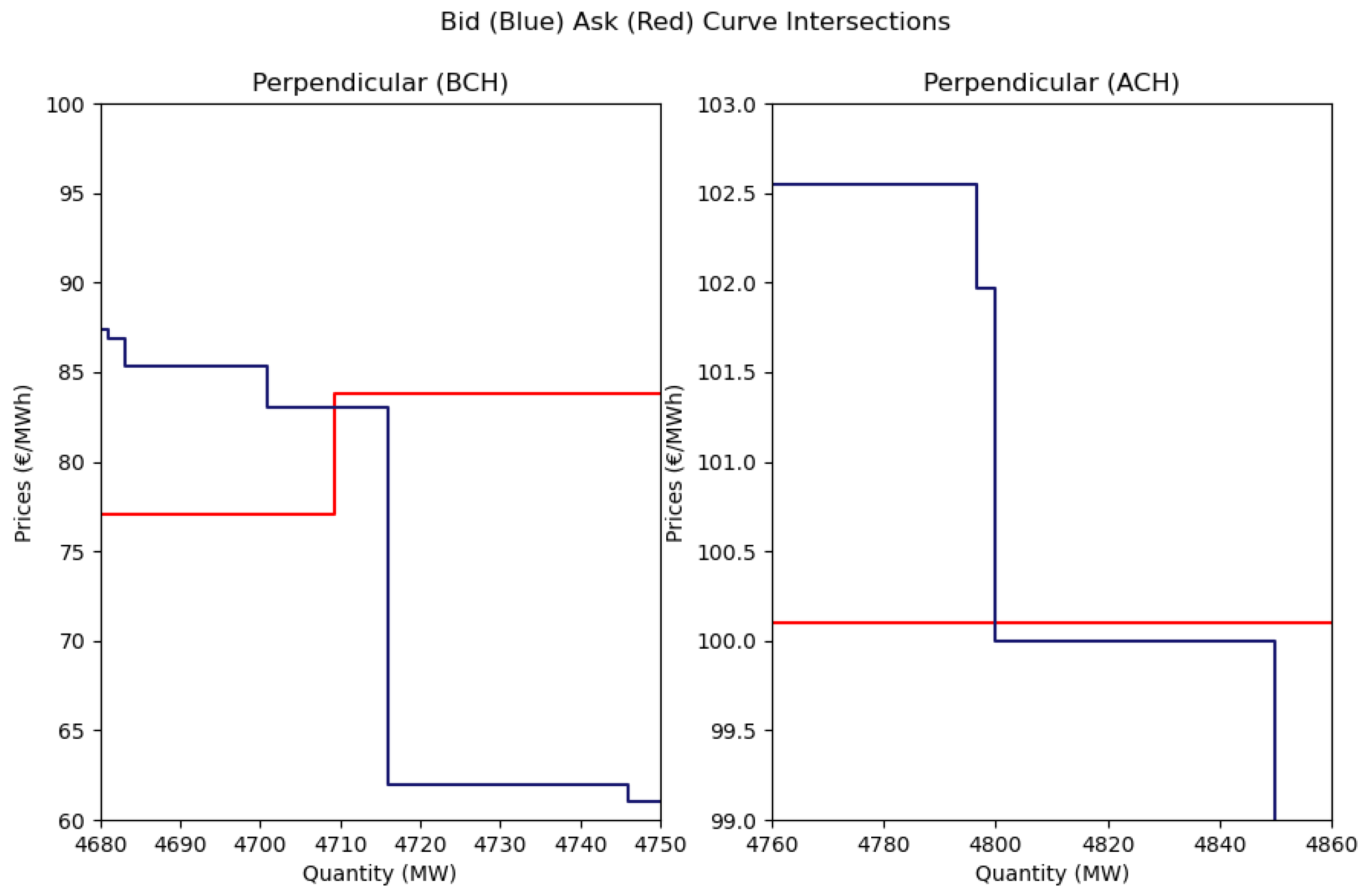
Figure A2.
Plot on the left (right) shows the Bid Ask Curve intersection for the I-SEM DA trading period 11pm-12am 30th Oct 2018 (12am-1am 31th Oct 2018).
Figure A2.
Plot on the left (right) shows the Bid Ask Curve intersection for the I-SEM DA trading period 11pm-12am 30th Oct 2018 (12am-1am 31th Oct 2018).
Appendix F. Speculators
AU_400137, AU_400139, AU_400143, AU_500104, AU_400140, SU_400314, AU_500101, AU_500126, AU_500012, AU_400118, AU_400100, AU_400122, AU_400002, AU_400128, AU_500110, SU_400136, AU_500114, AU_400103, AU_400138, AU_500109, AU_400003, AU_400006, AU_400101, AU_400135, SU_500082, AU_400105, AU_500001, AU_400005, AU_400010, AU_400141, AU_400111, AU_400125, AU_400106, AU_500115, AU_400114, AU_500121, AU_400112, AU_400132, AU_400119, AU_400116, AU_400113, AU_500122, AU_400134, AU_400117, AU_500105, AU_400011, AU_400009, AU_500113, AU_500111, AU_400136
Appendix G. Speculator Ex-Ante Trading
Consider the following hypothetical scenarios for speculator j in trading period i:
- Scenario 1: the speculator buys 100MW in DA and sells 100MW in IDA1; in this situation the profit and loss equals .
- Scenario 2: the speculator buys 50MW in DA and sell 150MW in IDA1; using equations 4 and 5 from Section 3.2 the profit and loss is given by . Rearranging, this is equivalent to .
That is, in both scenarios a proportion of the profit and loss is attributable to the loss or gain associated with taking opposing positions in ex-ante markets.
Appendix H. FuelType Notation
Categories for the FuelType field in the PUB_MnlyRegisteredCapacity file (Section 3.1) include wind, multi_fuel, gas, hdyro, peat, coal, pump_storage, biomass, oil, distillate and solar (this field can also be unpopulated). When presenting stacked area chart plots in Section 4, we combine some of the FuelType categories and utilise the following notation:
- Wind category represents those ResourceNames (market participants) where the FuelType is wind.
- Other category represents the units which don’t have a FuelType (and from their commercial behaviours appear in the main to be either demand or wind participants).
- Gas, MF category corresponds to gas and multi-fuel thermal generation units.
- Hyd, PS, P, Bio denote hydro, pumped storage, peat and biomass units.
- Speculator represents those units specified in Appendix F.
Appendix I. Buy Order Data Quantities
Figure A3.
Top plot presents speculator buy order quantities grouped by price interval and month. Bottom plot presents corresponding data for non-speculators. Values are in TWh, note the different y-axis scales.
Figure A3.
Top plot presents speculator buy order quantities grouped by price interval and month. Bottom plot presents corresponding data for non-speculators. Values are in TWh, note the different y-axis scales.
Appendix J. Parallel Shift
Figure A4.
Histogram of Price Difference (€/MWh), equation 6, for a +10MW parallel shift in the ask curve distinguishing between observations pre and post the structural market change. Note that Count is on a log scale.
Figure A4.
Histogram of Price Difference (€/MWh), equation 6, for a +10MW parallel shift in the ask curve distinguishing between observations pre and post the structural market change. Note that Count is on a log scale.
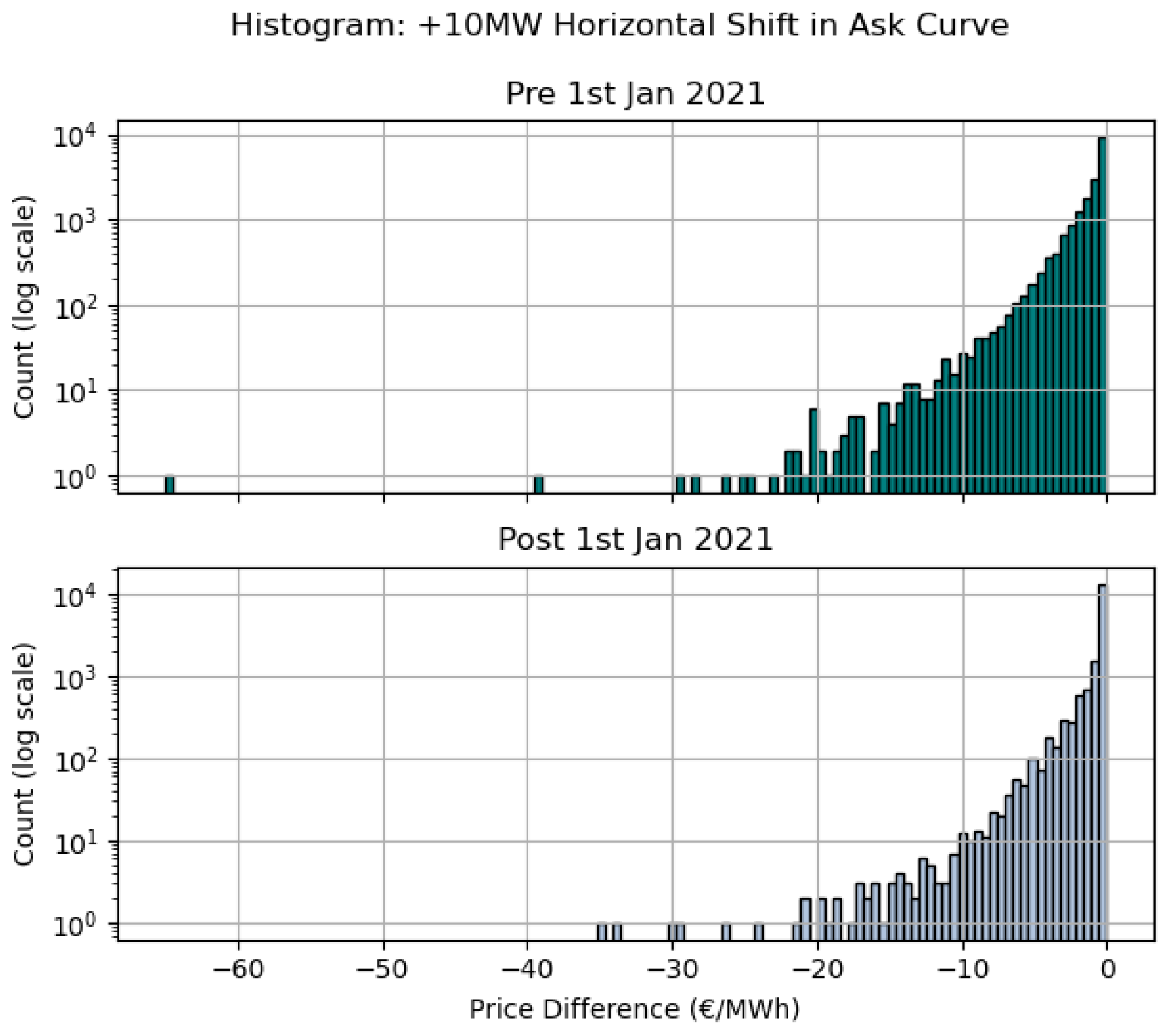
Figure A5.
Histogram of Custom Metric, equation 7, for a +10MW parallel shift in the ask curve distinguishing between observations pre and post the structural market change. Note that the Count is on a log scale.
Figure A5.
Histogram of Custom Metric, equation 7, for a +10MW parallel shift in the ask curve distinguishing between observations pre and post the structural market change. Note that the Count is on a log scale.
Appendix K. +1MW Parallel Shift in Ask Curve
The top (bottom) plot in Figure A6 shows the Price Difference (Custom Metric) values per trading period associated with a +1MW parallel shift in the ask curve. From the underlying data it is observed that in approximately 62% (12%) of all trading periods pre (post) 1st January 2021 application of a +1MW horizontal shift in the ask curve results in a changed market price. For those trading periods where the market price changes, there is an average reduction of 2.3% (0.7%) in the DA price pre (post) 1st January 2021.
Appendix L. Simulating Speculator DA Price Impact
To estimate the impact of a single speculator, j, on the DA price for trading period i, the process is as follows
- Retrieve all participant orders for trading period i from the relevant DA ETS Bid File. Convert each of the orders into price and quantity pairs.
- Take the buy price and quantity pairs from step 1 and combine them to produce an aggregated stepwise bid curve. Similarly, take the sell price quantity pairs and combine them to produce an aggregated stepwise ask curve.
- Adjust the stepwise bid and ask curves from step 2 as described in Appendix C.
- Use the bid and ask curves from step 3 to determine the intersection point/price.
- Repeat steps 1 to 4 but this time exclude the order data for speculator j.
We note that steps 1 to 4 can essentially be viewed as a validation step.
By way of example we apply this process to two contiguous trading periods for a particular speculator participant, the results are shown in Figure A7. The figure displays the bid and ask curves for two trading periods on 10th January 2019. The blue lines represent the curves excluding the speculator, while the red lines include them. Since the speculator only submitted sell orders, the red and blue bid curves are identical and hence overlap. For the 4am-5am trading period, the speculator placed sell orders of 4MW at €40/MWh and an additional 4MW at €50/MWh. In the 5am-6am period, similar sell quantities were submitted at €44/MWh and €54/MWh. The DA clearing prices for these periods were €59.16/MWh and €64.09/MWh, respectively. For 4am-5am, excluding the speculator shifts the ask curve to the left, resulting in a higher intersection price of €61.77/MWh. In contrast, for 5am-6am, while the ask curve shifts left again, the intersection price remains unchanged. Extending this analysis across all trading periods in which the speculator was active yields Figure A8. However, as noted in Section 3.3, in this broader analysis the assumption of a small change in the bid or ask curve does not always hold.
Figure A7.
Day-Ahead bid and ask curve intersections, with and without a single speculator, on 10th January 2019.
Figure A7.
Day-Ahead bid and ask curve intersections, with and without a single speculator, on 10th January 2019.
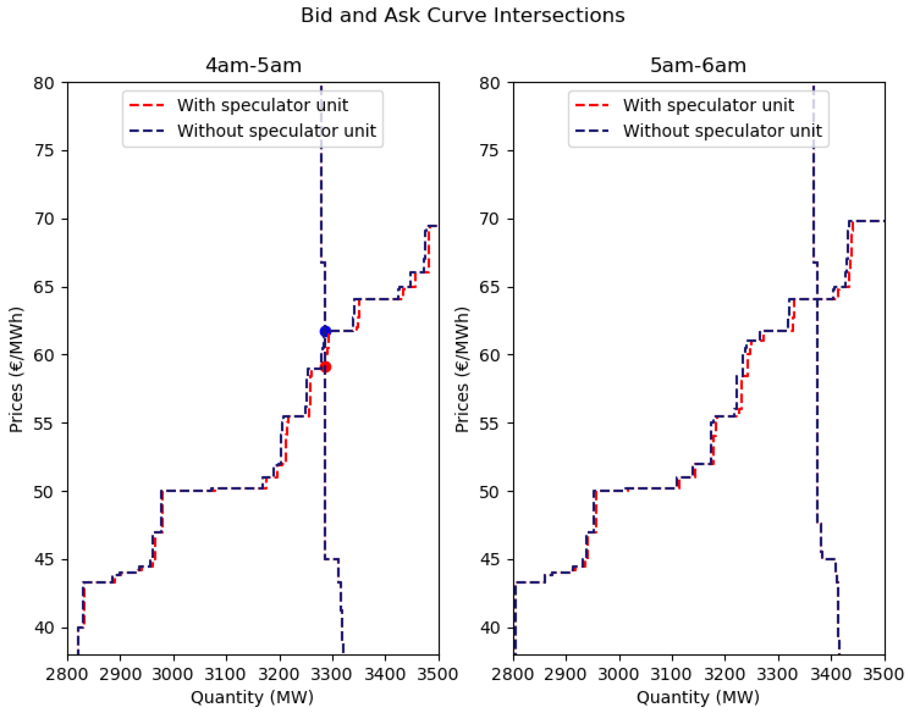
Figure A8.
Impact of a single speculator on the Day-Ahead bid and ask curve intersection. Negative (positive) x-axis values indicate sell (buy) speculator matched quantities. The y-axis represents the price difference: intersection price without the speculator minus the price with the speculator.
Figure A8.
Impact of a single speculator on the Day-Ahead bid and ask curve intersection. Negative (positive) x-axis values indicate sell (buy) speculator matched quantities. The y-axis represents the price difference: intersection price without the speculator minus the price with the speculator.
Appendix M. SEMO and SEMOpx
Pertinent reports/information from SEMOpx include
- Section 2.1.0.1, Structural Market Change, SEMOpx-Bidding.
- Section 3.1, Datasets, SEMOpx Data Publication Guide.
- Section 3.2, Empirical Analysis (Market Quantities), Market Summary 2019, Quarterly Report Q4 2020 and December 2022 Market Report.
- Section 3.2, Empirical Analysis (Speculator DA Order Evolution), SEMOpx DAM INFO 12 April 2022 and SEMOpx DAM INFO 30 August 2022.
Similarly, from SEMO, useful reference material includes
Appendix N. Market Prices
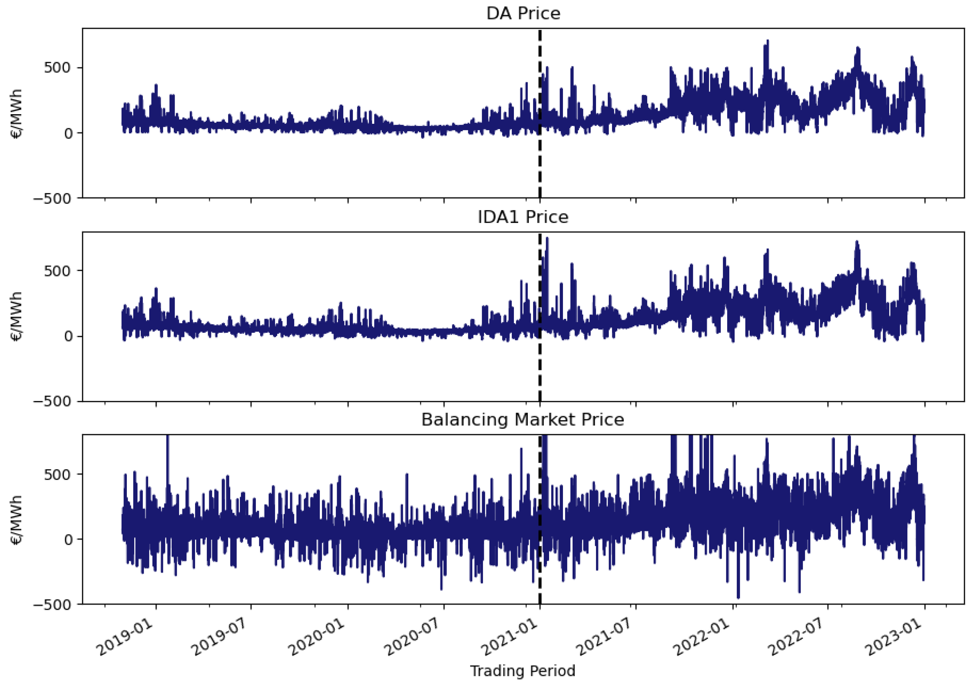
Figure A9.
Time series plots of Irish electricity DA, IDA1, and Balancing Market prices. The y-axis is cropped to the €/MWh range. From November 2018 to December 2022, the BM recorded 56 settlement periods with prices exceeding €800/MWh; the maximum BM price over the period was €4,800/MWh.
Figure A9.
Time series plots of Irish electricity DA, IDA1, and Balancing Market prices. The y-axis is cropped to the €/MWh range. From November 2018 to December 2022, the BM recorded 56 settlement periods with prices exceeding €800/MWh; the maximum BM price over the period was €4,800/MWh.
References
- Wolak, F.A. An empirical analysis of the impact of hedge contracts on bidding behavior in a competitive electricity market. International Economic Journal 2000, 14, 1–39. [Google Scholar] [CrossRef]
- Ito, K.; Reguant, M. Sequential markets, market power, and arbitrage. American Economic Review 2016, 106, 1921–1957. [Google Scholar] [CrossRef]
- Mayer, K.; Trück, S. Electricity markets around the world. Journal of Commodity Markets 2018, 9, 77–100. [Google Scholar] [CrossRef]
- Aggarwal, S.K.; Saini, L.M.; Kumar, A. Electricity price forecasting in deregulated markets: A review and evaluation. International Journal of Electrical Power & Energy Systems 2009, 31, 13–22. [Google Scholar] [CrossRef]
- Weron, R. Electricity price forecasting: A review of the state-of-the-art with a look into the future. International Journal of Forecasting 2014, 30, 1030–1081. [Google Scholar] [CrossRef]
- Ugurlu, U.; Oksuz, I.; Tas, O. Electricity Price Forecasting Using Recurrent Neural Networks. Energies 2018, 11. [Google Scholar] [CrossRef]
- Narajewski, M.; Ziel, F. Econometric modelling and forecasting of intraday electricity prices. Journal of Commodity Markets 2020, 19, 100107. [Google Scholar] [CrossRef]
- Canelas, E.; Pinto-Varela, T.; Sawik, B. Electricity portfolio optimization for large consumers: Iberian electricity market case study. Energies 2020, 13, 2249. [Google Scholar] [CrossRef]
- Harder, N.; Qussous, R.; Weidlich, A. Fit for purpose: Modeling wholesale electricity markets realistically with multi-agent deep reinforcement learning. Energy and AI 2023, 14, 100295. [Google Scholar] [CrossRef]
- Haase, M.; Zimmermann, Y.S.; Zimmermann, H. The impact of speculation on commodity futures markets–A review of the findings of 100 empirical studies. Journal of Commodity Markets 2016, 3, 1–15. [Google Scholar] [CrossRef]
- Tribe, E. BSC Insights: What is Driving Increases in Electricity Imbalance Volumes, 2019. Available online: https://www.elexon.co.uk/operations-settlement/balancing-and-settlement/elexon-insights-what-is-driving-increases-in-electricity-imbalance-volumes-july-2019/.
- Nyarko, S. 294/09: INVESTIGATIONS INTO NET IMBALANCE VOLUME CHASING (‘NIV CHASING’) IN GB ELECTRICITY MARKET, 2019. Available online: https://www.elexon.co.uk/documents/groups/panel/2019-meetings/294-september/294-09-investigations-into-niv-chasing-in-gb-electricity-market-shadrack-nyarko/.
- Parsons, J.; Colbert, C.; Larrieu, J.; Martin, T.; Mastrangelo, E. Financial Arbitrage and Efficient Dispatch in Wholesale Electricity Markets. SSRN Electronic Journal 2015. [Google Scholar] [CrossRef]
- Jha, A.; Wolak, F.A. Can financial participants improve price discovery and efficiency in multi-settlement markets with trading costs? Technical report, National Bureau of Economic Research, 2019.
- Mercadal, I. Dynamic competition and arbitrage in electricity markets: The role of financial players. JSTOR Sustainability Collection 2018. [Google Scholar] [CrossRef]
- Birge, J.R.; Hortaçsu, A.; Mercadal, I.; Pavlin, J.M. Limits to arbitrage in electricity markets: A case study of MISO. Energy Economics 2018, 75, 518–533. [Google Scholar] [CrossRef]
- Ullrich, C.J. Realized volatility and price spikes in electricity markets: The importance of observation frequency. Energy Economics 2012, 34, 1809–1818. [Google Scholar] [CrossRef]
- Erdogdu, E. Asymmetric volatility in European day-ahead power markets: A comparative microeconomic analysis. Energy Economics 2016, 56, 398–409. [Google Scholar] [CrossRef]
- Mayer, K.; Trück, S. Electricity markets around the world. Journal of Commodity Markets 2018, 9, 77–100. [Google Scholar] [CrossRef]
- Hellström, J.; Lundgren, J.; Yu, H. Why do electricity prices jump? Empirical evidence from the Nordic electricity market. Energy Economics 2012, 34, 1774–1781. [Google Scholar] [CrossRef]
- Sensfuß, F.; Ragwitz, M.; Genoese, M. The merit-order effect: A detailed analysis of the price effect of renewable electricity generation on spot market prices in Germany. Energy policy 2008, 36, 3086–3094. [Google Scholar] [CrossRef]
- Ciarreta, A.; Espinosa, M.P. Market power in the Spanish electricity auction. Journal of Regulatory Economics 2010, 37, 42–69. [Google Scholar] [CrossRef]
- Ziel, F.; Steinert, R. Electricity price forecasting using sale and purchase curves: The X-Model. Energy Economics 2016, 59, 435–454. [Google Scholar] [CrossRef]
- Bask, M.; Widerberg, A. Market structure and the stability and volatility of electricity prices. Energy Economics 2009, 31, 278–288. [Google Scholar] [CrossRef]
- Fabra, N. Reforming European electricity markets: Lessons from the energy crisis. Energy Economics 2023, 126, 106963. [Google Scholar] [CrossRef]
- Eurelectric. How are EU electricity prices formed and why have they soared? 2022. Available online: https://www.eurelectric.org/in-detail/electricity_prices_explained/ (accessed on 8 June 2025).
- EFET. EFET Insight into Marginal Pricing in Wholesale Electricity Markets, 2022. efet.org/files/documents/20220222%20EFET_Insight_02_marginal_pricing.pdf.
- Collins, J.; Amann, A.; Mulchrone, K. Why gas and electricity prices in Ireland are so closely linked, 2022. Available online: https://www.rte.ie/brainstorm/2022/0727/1312565-ireland-gas-electricity-prices-correlation/.
- REMA. Review of electricity market arrangements, 2022. Available online: https://www.gov.uk/government/consultations/review-of-electricity-market-arrangements.
- The Guardian. ‘I’ve fallen out with people’: the bruising debate over UK zonal energy pricing. The Guardian. 2024. Available online: https://www.theguardian.com/money/2024/oct/07/ive-fallen-out-with-people-the-bruising-debate-over-uk-zonal-energy-pricing (accessed on 23 May 2025).
- Ritchie, H.; Roser, M.; Rosado, P. Energy. Our World in Data, 2022. Available online: https://ourworldindata.org/energy.
- ElectroRoute. Electroroute Brexit Commentary, 2020. Available online: https://electroroute.com/interconnecting-the-dots-on-future-brexit-arrangements/.
- SEMOpx-Bidding. SEMOpx-Bidding, 2021. Available online: https://www.semopx.com/documents/training/SEMOpx-Bidding.pdf.
- EUPHEMIA. EUPHEMIA Public Description Single Price Coupling Algorithm, 2020. Available online: http://www.nemo-committee.eu/assets/files/euphemia-public-description.pdf.
- Madani, M. Single Day-Ahead Coupling: important successes for the Euphemia Lab, 2020.
- NEMO. CACM Annual Report 2021, 2021.
- Bharatwaj, V.N.; Downey, A. Real-Time Imbalance Pricing in I-SEM - Ireland’s Balancing Market. In Proceedings of the 2018 20th National Power Systems Conference (NPSC); 2018; pp. 1–6. [Google Scholar] [CrossRef]
- Elexon. A guide to electricity imbalance pricing in Great Britain, 2020.
- IEA. Covid-19 impact on electricity, 2021.
- Kuik, F.; Adolfsen, J.F.; Lis, E.M.; Meyler, A. Energy price developments in and out of the COVID-19 pandemic – from commodity prices to consumer prices, 2022.
- SEMOpx. SEMOpx Market Platform, 2023. Available online: https://www.semopx.com/.
- SEMO. Single Electricity Market Operator (SEMO), 2023. Available online: https://www.sem-o.com/.
| 1 | While Virtual Bidding does not exist in European electricity markets, participants may engage in similar speculative strategies through other mechanisms. For example, in the British market, Net Imbalance Volume (NIV) chasing allows traders to profit from spreads between ex-ante prices and balancing market prices [11,12]. Similarly, [2] document speculative behaviour by wind generators in the Iberian market, who exploit price differences across sequential trading periods. |
| 2 | They note: “When financial participants’ ability to arbitrage the premium is limited, we find evidence suggesting that for large actors it may be more profitable to use their bids to increase the value of related instruments instead of arbitraging the premium.” |
| 3 | |
| 4 | IDA1/IDA2/IDA3 auctions cover the [11pm D, 10:30pm D+1]/[11am D+1, 10:30pm D+1]/[5pm D+1, 10:30pm D+1] time horizons respectively. |
| 5 | ex-ante in this context means occurring before the delivery period, ex-post means that it occurs after the delivery period. |
| 6 | For the British electricity market, Elexon provides similar imbalance pricing guidance in [38]. |
| 7 | |
| 8 | As of July 2021 SEMOpx have simplified matters by publishing a single BidAskCurve file for each ex-ante auction with the bid and ask information per trading presented in €/MWh. Prior to that date, SEMOpx would publish two BidAskCurve files for each ex-ante auction, one containing information in £/MWh relating to the Northern Ireland (NI) marketarea and the other containing information in €/MWh relating to the Republic of Ireland (ROI) marketarea. |
| 9 | The maximum DA price has increased in stages from €3000/MWh to €5000/MWh. We take this into account in our empirical analysis by assuming all orders are capped at the €3000/MWh level. |
| 10 | For details on the FuelType notation used in Figure 1 see Appendix H. |
| 11 | Close to € billion worth of energy has been traded in the ex-ante markets over the same timeframe, see Appendix M. |
| 12 | The associated p-value is . |
| 13 | ResourceName is an identifier that is unique to each market participant; FuelType categories include wind, multi_fuel, gas, hdyro, peat, coal, pump_storage, biomass, oil, distillate, solar. |
| 14 | Picking an arbitrary threshold, if a ResourceName is buying (selling) > 92.5% of trading periods it is active in the DA, then we treat it as a demand (supply) unit and exclude it. |
| 15 | Defined as “a Simple Sell Order or a set of Simple Sell Orders submitted by an Exchange Member in respect of a Unit, covering one or more Trading Periods on a specified Trading Day, and which is subject to: (a) a Minimum Income Condition (with or without a Scheduled Stop Condition) and/or (b) a Load Gradient Condition".
|
Figure 1.
The top plot presents Irish electricity market DA Sell Order Quantities, the bottom plot presents DA Sell Matched Quantities. Values are in TWh and the data has been grouped by FuelType and month. The dashed vertical line indicates the point in time at which the structural market change related to Brexit occurred.
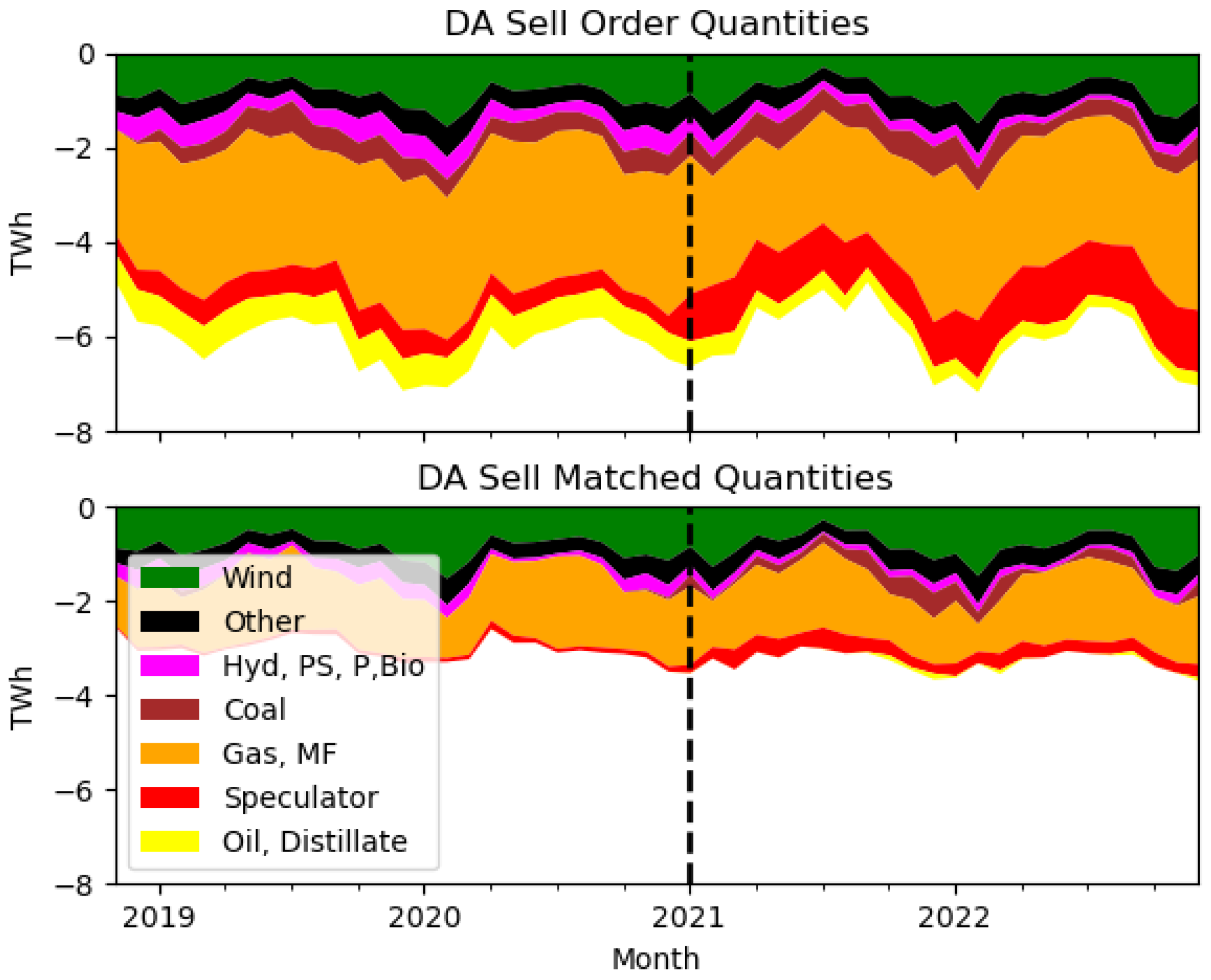
Figure 2.
Top plot shows the the percentage of marginal observations in the DA market grouped by FuelType and month. Bottom plot shows the percentage of DA bid and ask curve intersection types by month.
Figure 2.
Top plot shows the the percentage of marginal observations in the DA market grouped by FuelType and month. Bottom plot shows the percentage of DA bid and ask curve intersection types by month.
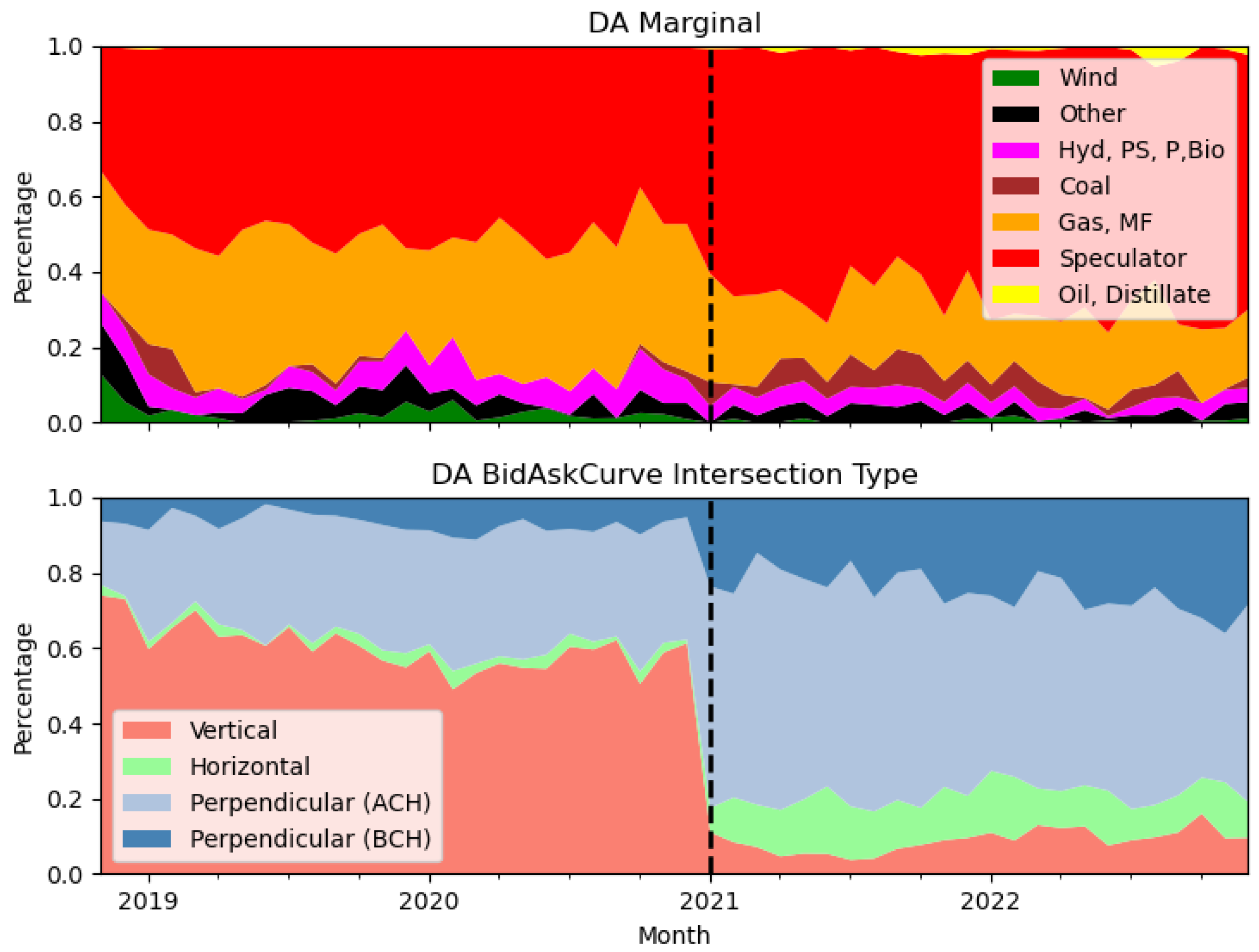
Figure 3.
Top plot presents speculator sell order quantities grouped by price interval and month. Bottom plot presents corresponding data for non-speculators. Values are in TWh, note the different y-axis scales.
Figure 3.
Top plot presents speculator sell order quantities grouped by price interval and month. Bottom plot presents corresponding data for non-speculators. Values are in TWh, note the different y-axis scales.
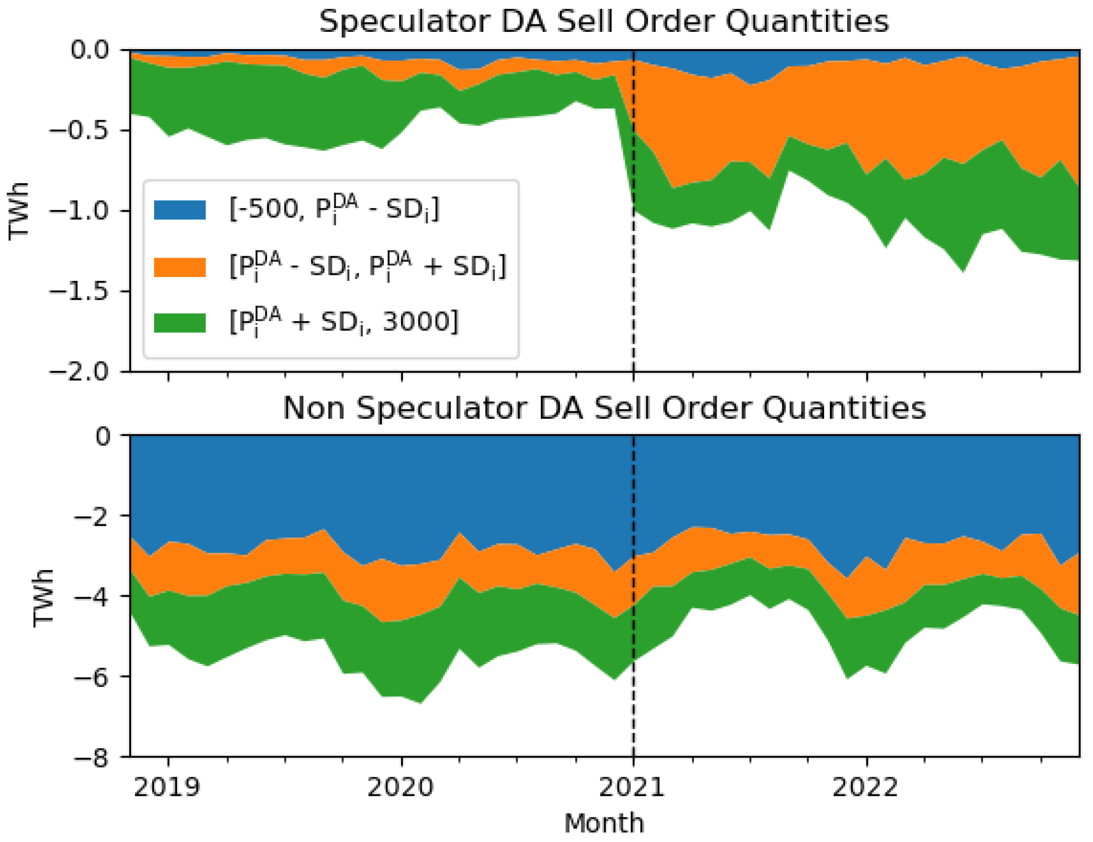
Figure 4.
Scatter plot of speculator DA and IDA1 matched quantities, as defined in equations 1 and 2. Values are in MW.
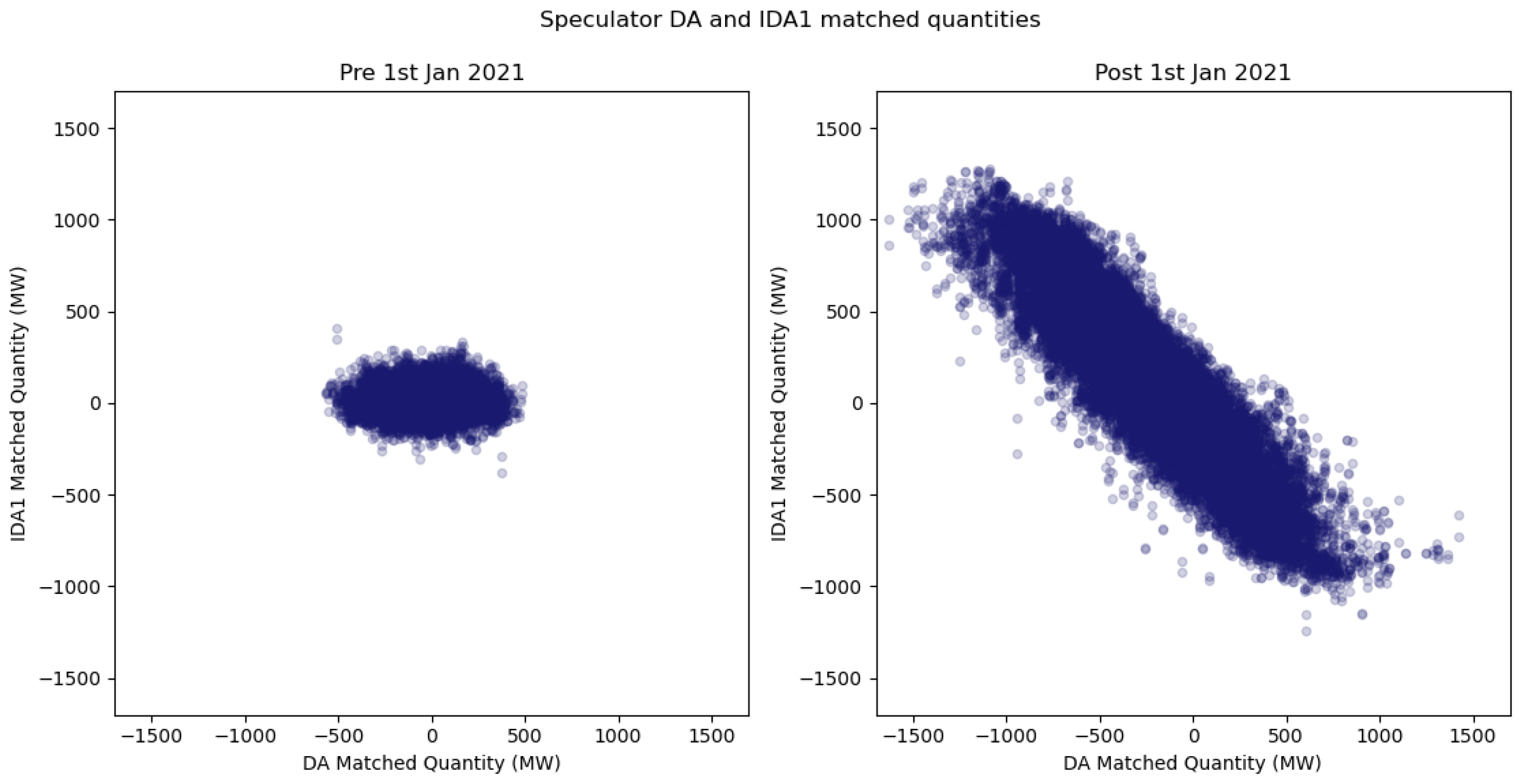
Figure 5.
Scatter plot of speculator DA matched and Balancing Market quantities, as defined in equations 1 and 3. Values are in MW.
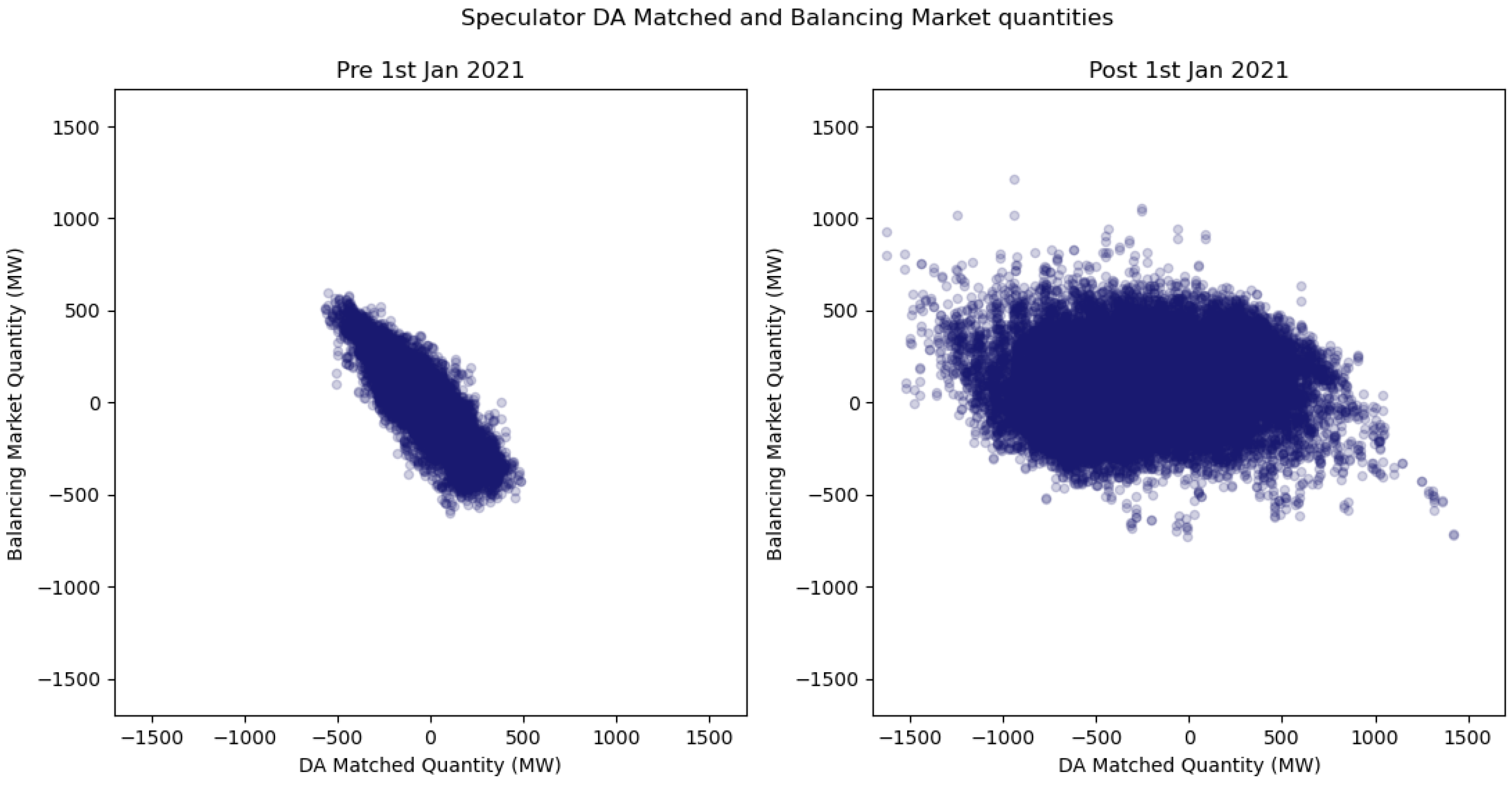
Figure 6.
Speculator time series plots for a sample timeframe (units in MW). The top plot corresponds to equations 1 and 2, with the latter inverted (i.e., multiplied by ). The middle plot corresponds to equation 3. In the bottom plot, Speculator DA Buy and Sell Matched Quantities are shown separately.
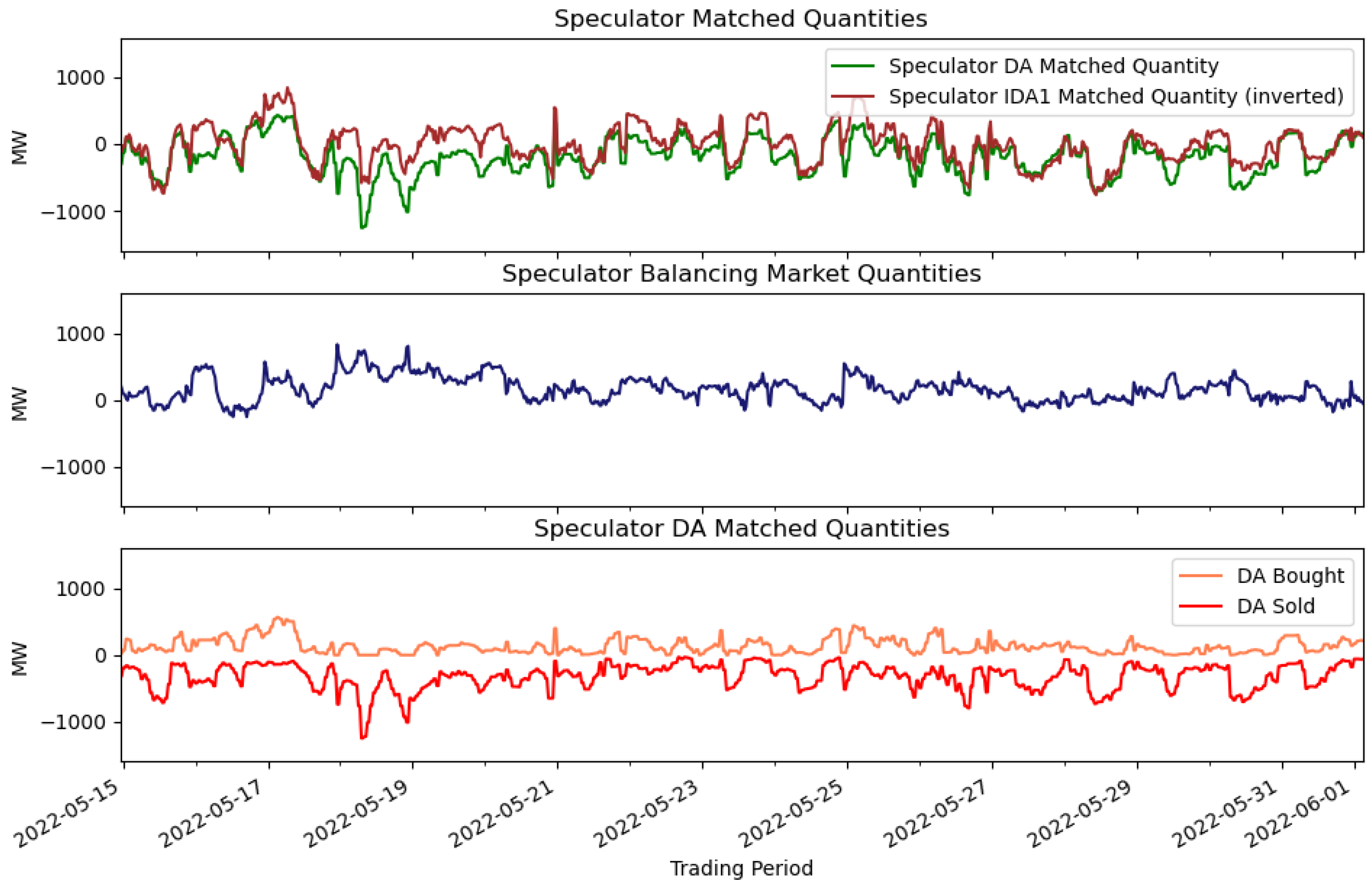
Figure 7.
Percentage of trading periods per day where the Price Difference values, defined by equation 6, are €0/MWh.
Figure 7.
Percentage of trading periods per day where the Price Difference values, defined by equation 6, are €0/MWh.
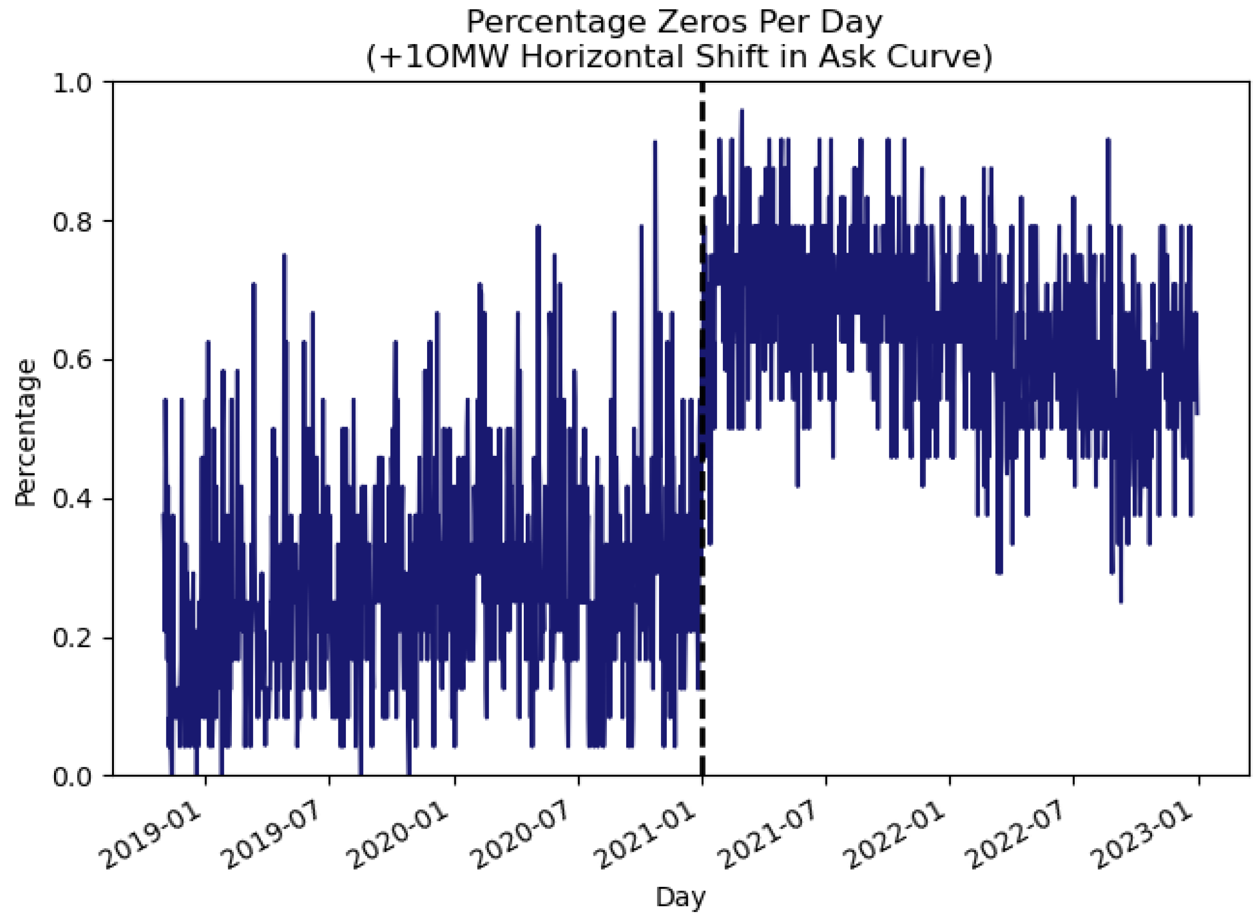
Figure 8.
Impact, per trading period, of a +10MW horizontal shift in the ask curve. Values in top plot are given by equation 6, values in bottom plot are given by equation 7.
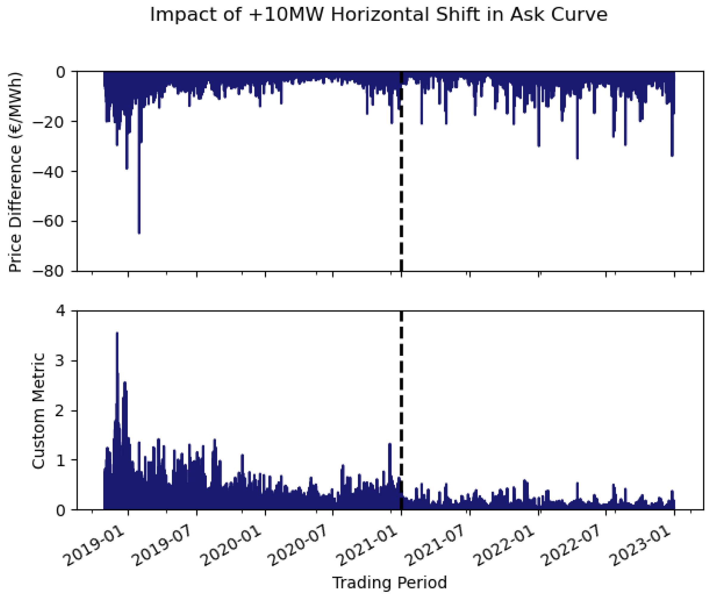
Figure 9.
Scatter plot showing the impact, per trading period, of a +10MW horizontal shift in the ask curve distinguishing between observations pre and post 1st January 2021.
Figure 9.
Scatter plot showing the impact, per trading period, of a +10MW horizontal shift in the ask curve distinguishing between observations pre and post 1st January 2021.
Disclaimer/Publisher’s Note: The statements, opinions and data contained in all publications are solely those of the individual author(s) and contributor(s) and not of MDPI and/or the editor(s). MDPI and/or the editor(s) disclaim responsibility for any injury to people or property resulting from any ideas, methods, instructions or products referred to in the content. |
© 2025 by the authors. Licensee MDPI, Basel, Switzerland. This article is an open access article distributed under the terms and conditions of the Creative Commons Attribution (CC BY) license (http://creativecommons.org/licenses/by/4.0/).
Copyright: This open access article is published under a Creative Commons CC BY 4.0 license, which permit the free download, distribution, and reuse, provided that the author and preprint are cited in any reuse.


