
Submitted:
04 November 2025
Posted:
06 November 2025
You are already at the latest version
Abstract
This paper aims to provide a detailed insight into the wave loads induced by a dam break flow over a dry horizontal bed under well controlled laboratory conditions. The setup used is based on the one in [1], with the addition of rigid obstacles, that lead to three dimensional dynamics. The focus is on wave impact pressure, for which measurements at the downstream wall at three different locations placed at the same height but at different transverse positions have been recorded. Pressure peak maxima are identified and the pressure impulses are computed. A statistical analysis of the experimental data generated in the campaign is performed. Repetitions of each case have been carried out until convergence of the statistics is observed. Comparisons between the configurations studied and against previous experimental campaigns, involving two-dimensional dam breaks, are provided, highlighting the deviations introduced by the obstacles. The data can be used to validate and calibrate numerical solvers aimed at computed wave induced structural loads.
Keywords:
dam break
; impact pressure
; impulsive loads
; 3D flows
; sloshing
1. Introduction
The dam break experiment has often been addressed in the literature as a validation case for many CFD codes, e.g. [2,3,4,5,6]. Despite the fact that an extensive discussion of dam break wave kinematics can be found in the literature, there is some lack of data describing its dynamics, which is useful when assessing certain types of impact flows like those found in slamming and green water events [7,8]. In 1999, Zhou et al. [9] validated their numerical scheme using an experimental work. In that paper, they provided a description of dam break wave kinematics as well as data on wave impact pressures on a solid vertical wall downstream the dam. The details on experimental setup and on applied force transducers were later published in [10]. The geometry proposed therein is reproduced in the present work. Also, this setup was further used in other experimental campaigns, as those by Wemmenhove et al. [11] or Kleefsman et al. [12]. The former repeated and slightly altered experiments of Zhou [9], the latter presented a fully three-dimensional dam break problem.
Research on dam break flow dynamics was also conducted by Bukreev et al. who studied the forces exerted by the dam break wave on vertical structures downstream the dam [13,14]. A similar test case was considered by Gómez-Gesteira et al. [15] and by Greco et al. [16], who studied that case to validate their computational model. Other computational works focused on measuring forces considering particular geometries with obstacles.
While literature on the dam break is not scarce, there are few studies treating dam breaks with three-dimensional flows, specially when experiments are involved, e.g. [17,18]. On the contrary, most works have investigated the problem using CFD simulations. In [19], the Finite Volume method (as implemented in OpenFoam software) was applied to study the problem of an inclined dam break (considering different slopes) with an obstacle. The OpenFoam software was also used in [20], which addresses the dam break with an obstacle. Only a two dimensional case is studied therein. In [21], a three dimensional flow around fixed obstacles was numerically studied using Smooth Particle Hydrodynamics (SPH).
Among the few studies addressing the problem under an experimental perspective, except for few cases such as [22] or [23], that provide a complete set of data on kinematics of series of several tests, there is a lack of a thorough discussion on the repeatability of variables that are measured during these events. In [17], a three-dimensional flow in a dam break with an obstacle was experimentally studied. Three repetitions of the experiment were carried out. The flow was characterised through water level measurements at five different locations and velocity measurements using an acoustic Doppler velocimeter. No assessment of the convergence of the statistical parameters was considered. However, a probabilistic approach is crucial to properly describe the fluid dynamics. This is so because dam break flows are characterised by leading to impact events on any downstream walls or obstacles. Any small deviation on external conditions (gate speed, gate induced vibrations, temperature of the fluid, etc.) from one test to the next may induce significant variations on the values of the flow fields (pressure in particular) measured in the experiments.
This paper aims to provide a detailed insight into the dynamics of the dam break flow over a dry horizontal bed under well controlled laboratory conditions when obstacles inducing three dimensional flows are involved. In order to do so, an experimental setup similar to that used by Zhou et al. [9] and Buchner [10], widely considered for validation purposes (e.g. [24,25]), has been used. Zhou et al. published their experiments in a conference paper [9] in 1999 and they were later (2002) published as a journal paper by Lee, Zhou her/himself and Cao [26]. These references [9,26] contain the same experimental data and are cited indistinctly in the present paper. The facility used in the present research was already used by Lobovsky et al. [1] to perform statistical analysis of simple dam break (without obstacles) experimental data. That facility has been adapted to include an obstacle, in different positions, to induce three dimensional flows.
Special attention has been paid to measurements of the impact pressure of the downstream wave on the flat vertical wall. In order to address the repeatability of the experiments, a large set of measurements is performed under the same experimental conditions.
The main originality and outcome of this research resides in providing a probabilistic description of the impact pressure, of the rise time and of the pressure impulse, and compare them with relevant data from the literature.
The obtained results from a thorough statistical analysis of the experimental data provide novel information about the pressure measurements in 3D dam break test cases and complement the knowledge of the previously published studies discussed above.
In summary, the three main objectives of this work are:
- Provide a probabilistic description of the measurements (pressure peaks and rise times), including mean, median, standard deviations, and confidence intervals. The idea is that these data can be used to validate 3D simulations of dambreak flows.
- Compare the results obtained in the two configurations studied among them (both with significant 3D effects) and more importantly also with the 2D results published in [1].
- Provide data for other authors with need to validate their models for wave induced structural loads. To this aim, the figures (in MATLAB format) and abundant movies can be downloaded from this link: https://short.upm.es/q29zb.
The paper is organised as follows: first, the experimental setup and methodology, together with the test matrix, are discussed. Next, the experimental results are presented and analysed. Also, these different cases are compared with previous results in the literature. Finally, the paper is closed by collecting some conclusions and presenting future work.
2. Experimental Setup and Methodology
2.1. Experimental Setup
The dam break experimental setup was built and installed at the sloshing laboratory of the research group CEHINAV at UPM-ETSIN facilities. In this laboratory, in a previous experimental campaign [1], a statistical study of the pressure measurements at the end wall was performed for 100 repetitions and two different filling levels. The setup used used in this paper is based on the one used in [1], with the addition of rigid obstacles that induce 3D flows. Figure 1 shows the experimental device.
In order to induce 3D flow, a stainless steel obstacle has been placed at (see Figure 2). As shown in Figure 3, the obstacle is composed by two parts: a bracket and a plate. The plate is a rigid sheet with height D, equal to the tank height, breadth b, equal to half the tank breadth, B, and thickness equal to . The tank breadth, B, is equal to 150 mm, as shown in Figure 2.
The bracket consists of a metal sheet with two longitudinal cavities which allows to position the plate anywhere in the transverse dimension of the tank. Four screws attach the plate to the bracket, with the bracket being attached to the tank by means of welded splints and two other fasteners. Thanks to these mechanisms, we can consider both the plate and the bracket as static rigid structures with no relative motion to the tank.
The thickness of the plate has been selected to ensure that the displacement at its tip does not exceed 1 mm when impacted by the dam break flow, allowing us to consider it a rigid body. When placed close to the tank wall, petroleum jelly was applied in the resulting gap in order to prevent any lateral leaks.
The liquid used for the experiments is fresh water (see properties in Table 1). Before each test, the water is heated to a reference temperature (C) and the temperature is checked using a standard thermometer with an uncertainty of ± 0.1 °C. In this way, we assure that the water exhibits the same mechanical properties in each test. The water was dyed using a tiny amount of Fluorescein Sodium (C.l. 45350) PA to have a better visualization of the free surface.
2.2. Data Acquisition
The data acquisition system consists of the pressure sensors to measure the downstream impact, the potentiometer to control the gate speed and the cameras to record the free surface evolution of each test.
Three Piezo-resistive pressure sensors (KULITE XTL-190 series) with sensing diameter of mm have been used. A NI-PCI 6221 card allows to amplify the signal before the A/D conversion. The sampling rate of the digital signal is 20 kHz. Sensors feature an effective full-scale output (FSO) of 400 mb. As displayed in Figure 2, the pressure probes are labeled as 1, 2 and 3 and the corresponding pressure signals are , and respectively. Sensor 1 is located close to the front wall at 112.5 mm, sensor 2 is located at the middle of the downstream wall at 75 mm and sensor 3 is placed close to the back wall of the tank at 37.5 mm. The uncertainty of the bias in the pressure measurements is of 0.5 mb, the same as in experimental campaign conducted in [1]. Taking into account the pressure ranges, these measurements are comparable in accuracy to those reported by [27].
A multiturn potentionmeter has been installed at the dry side of the gate to measure the gate motion, see Figure 1, label (3). The potentionmeter signal V (in Volts) is converted to distance and then its derivative with respect to time allows the calculation of the gate speed. The potentiometer is connected to the DAC analogical card NI-9224 that amplifies the voltage. The potentiometer signal is also used to set the time zero for the pressure measurements in each test.
The experiments are recorded from two different views: one recording the front of the tank and another one recording a zenital view of the tank. The video footage obtained from the test images is used to identify the free surface shape and the most relevant events. The camera devices present a resolution of 1080p and a 240 fps frame rate.
The video frames and the pressure sensors are correlated with the potentiometer signal allowing to have a common time reference for all signals. In the synchronization process two characteristic times are taken into account:
- is the instant when the gate is released. All signals are referenced to being this instant the beginning of the experiment s.
- is the instant when the flow impacts the rigid plate obstacle.
The initial instant is given by the potentiometer, and this time is correlated with the front camera that records the tests. Once the correlation between the front camera and the potentiometer has been made, can be derived from the video recordings having an uncertainty of ± 1 frame (or ± 0.0042 s). In addition, to provide a more detailed visualisation of the flow during the obstacle impact, a secondary camera has been installed to present a zenital view of the flow impacting the rigid plate. This secondary camera has been placed at the top of the setup. The time synchronization with the secondary camera is performed by using the time obtained from the frontal camera.
2.3. Post-Processing Methodology
The signals considered are the pressure measurement of sensors 1, 2 and 3: , , and the measurement of the gate displacement V. The gate displacement signal V is used to determine and the maximum velocity of the gate, which is always of the order of m/s. Once the pressure signals have been time referenced, from the collected pressure signals 4 magnitudes can be derived in the post-processing step: the maximum pressure peak P, the rise time , decay time and pressure impulse I. A MATLAB® code has been used to perform all the post-processing steps.
The maximum pressure peak is calculated as:
The maximum pressure peak calculated in equation 1 is computed close in time to the impact event in order to avoid spurious pressure peaks coming from secondary splashes later in the experiment.
The rise time and decay time of a pressure signal are calculated as shown in Figure 4. The definition of the rise time is taken from ISOPE 2012 benchmark [27]. The rise time is defined equal to twice the time that the pressure signals takes to rise from its half-maximum value to the maximum peak value P. Equivalently, the decay time is defined as twice the time it takes to the pressure signal to decay from its maximum value P to its half-maximum value .
The rise time was calculated for the signals coming from all sensors but the decay time has only been calculated for sensor 1 () in the asymmetric configuration since it is the only pressure signal impulsive enough to allow the definition of the decay time. The impact time is defined as the sum of the rise time plus the decay time.
The pressure impulse is defined as:
As it was mentioned before and will be shown in detail later in the paper, since most of the registered signals were not impulsive enough, the definition of the total impact time was not possible for those cases, therefore not allowing the calculation of the pressure impulse I. This calculation was performed for sensor 1 in the asymmetric configuration. The integral of equation 2 is computed using the trapezium rule.
2.4. Test Matrix
Before conducting the experimental campaign, a validation stage with no obstacle was carried out to check that the measured pressure signals are consistent with those reported in [1]. The data collected for the 10 performed repetitions were found to fall in the range of 2. 5% - 97. 5% in the 2014 study.
The experimental tests presented in this paper include an obstacle that induces 3D flow. The width of the obstacle plate is b and the total cross-sectional length is B as indicated in Figure 5. We can define the ratio between the obturated b and total cross-sectional lengths B as , a non-dimensional number that represents the level of blockage of the channel. All tests present the same blockage level of .
Figure 5 shows the 2 different configurations tested in this paper. In the asymmetrcial configuration, the plate is placed at a distance measured from the right lateral wall . In this configuration the flow is expected to collide with the plate resulting in an asymmetrical flow with a lateral wave that will later impact the wall at which the pressure probes are measuring. In the symmetrical configuration, the center of the plate is located at which will generate a symmetrical flow with two lateral waves after the dam break flow collides with the plate.
3. Results: Asymmetric Configuration
The results presented in this section have been obtained for a liquid height of mm, using water as liquid (see Table 1) and placing the obstacle in the asymmetric configuration as described in Section 2 (see Figure 5).
3.1. Experimental Snapshots
Figure 9 and Figure 10 show the flow evolution during one experimental test. The liquid starts from the hydrostatic state (a.1) and when the gate is released (b.1), a downstream wave is generated due to the action of gravity (c.1). This primary wave travels along the dry bed (a.2, b.2 and c.2) displaying flow structures that are mostly laminar. Up until this point the flow evolution is similar to the one presented in the previous study with no obstacle [1]. Then, the wave encounters the rigid obstacle (d.1 and d.2) which redirects the flow to the lateral wall of the reservoir (e.1 and e.2). The generated jet due to the impact with the obstacle moves forward parallel to the lateral walls (f.1 and f.2) until it reaches the back wall and impacts the measuring area (g.1 and g.2). After the impact, a secondary wave is produced that travels back (h.1 and h.2) and impacts the obstacle from the back side (i.1 and i.2).
3.2. Pressure Measurements
The impact pressure was measured using three sensors on the vertical wall at the end of the opposite side of the water reservoir, as described in Section 2. The arrangement of the sensors is indicated in Figure 2. A typical impact event signal, as recorded by the three sensors, can be seen in Figure 11. The recorded pressure p is non-dimensionalized using the hydrostatic pressure at the bottom of the reservoir .
As shown in Figure 11, the highest peak is recorded for sensor 1 which is the sensor that recieves the full impact of the incoming water wave. Then, the wave impacts sensor 2 which is why it records a lower peak and finally it hits sensor 3 which records the lowest pressure peak and it is also delayed in time when compared to the other two.
In Figure 12, the pressure time histories of sensor 1 are shown along with the median and the 97.5 % and 2.5 % percentiles. The mean of the maximum pressures is . We see that the confidence intervals considerably increase for the tail of the signal, something that did not happen in the previous study conducted in [1] where no obstacle was placed. This could indicate that the flow after the impact is much more complex due to the rigid obstacle presence and the nature of the 3D flow. The maximum pressure peaks are notably localised in time being the mean value of the impact event at .
Following the same analysis, Figure 13 shows the pressure time histories of sensor 2 for the 25 repeated tests along with the median and confidence intervals. We see a much less violent impact event when compared to the measurements of sensor 1 with a mean of the maximum pressures of . Also, the impact event is more dilated in time showing two maxima. The absolute maximum is found for the first peak for the majority of the tests but there are a few tests where the absolute maximum has been found for the second pressure rise. It is also worth noting that the confidence intervals become thinner close to the tail of the signal whereas close to the impact event they become wider. This observation could indicate that when the impact is registered in sensor 2 there is already a complex and chaotic behaviour of the impacting flow due to 3D characteristics of the incoming wave. The maximum pressure peaks are not as localised as for sensor 1, presenting a mean time value of .
Analogously, Figure 14 displays the pressure time histories of sensor 3 for the 25 tests along with the median and the confidence intervals. We see that the impact event registered by sensor 3 is the least violent among the three sensors with a mean of the maximum pressures of . Furthermore, we see that the pressure rise is very delayed in time and sometimes does not even register an impact event. This pressure rise is also remarkably scattered showing a big dispersion of the maximum pressure peaks with a mean time value of .
The dispersion of pressure peak measurements is something that has received attention in the literature [28,29,30]. In our study the experiment was repeated 25 times and the Empirical Cumulative Distribution Functions (ECDF’s) of the pressure peaks are displayed in Figure 15. We see that the largest dispersion is found for sensor 1 which is the sensor that registers the highest pressure peak values. Then, the dispersion decreases for sensor 2 and then sensor 3. The dispersion of the maximum pressure peaks decreaseases with the pressure peak intensity.
The values of the maximum pressure peaks along with the median for the preformed 25 tests is shown in Figure 16. The medians in dimensional units are 48.61 mb, 29.96 mb and 20.85 for sensors 1, 2 and 3 respectively. Even if the sensors are located at the same height they do not record the same pressure peak due to the three-dimensionality of the flow. The intensity of the peaks decreases in accordance with their relative position with respect to the rigid obstacle, registering higher pressure peaks if the sensor is located in the gap between the plate and the wall and lower peaks if the sensor is located behind the plate. Following the procedure described in [31], the Reverse Arrangement Test (RAT) was carried out taking as random variable the maximum pressure peaks displayed in Figure 16. For a significance level of 0.05 the null hypothesis is accepted indicating that there is a sign of independence among the 25 registered pressure peaks of each sensor.
In Figure 17 we can see the time instants of the maximum pressure peaks, previously displayed in Figure 16, along with their median values. We observe that the highest time is recorded for sensor 3 then sensor 2 and finally sensor 1 (presenting an inverse relationship with respect to the trend shown in Figure 16). The medians of the maximum pressure times in dimensional units are 0.45, 0.48 and 2.43 seconds for sensors 1,2 and 3 respectively. We also see an increase of the dispersion of the data as we go from sensor 1 to sensor 3. This observation is directly related with the fact that the wave takes longer times to reach sensor 3 and it is more fragmented and presents a more complex flow since it has already impacted sensors 1 and 2.
The maximum pressure peaks registered by sensor 1 are correlated with the ones measured in sensors 2 and 3. These correlations are displayed in Figure 18. We see a positive relationship for both correlations, being the one between sensors 1 and 3 stronger with a linear correlation factor of 0.6006 and the one between sensors 1 and 2 somewhat weaker with a correlation factor of 0.3678. The positive correlation between the pressure sensors is expected since the impacting wave hits first sensor 1 and then the other two, therefore, a more violent pressure impact would be registered in all the sensors in a consistent manner. However, the low value of the linear correlation factor may indicate that due to the intricate nature of the three dimensionality of the flow, we do not always register high pressure peaks for all sensors when energetic wave impacts occur.
3.3. Rise Times, Decay Times and Pressure Impulse
As explained in Section 2, from the pressure time histories the rise time, decay time and pressure impulse can be calculated (see Figure 4). The rise time definition was possible for all three sensors, however, the decay time and pressure impulse calculation was only possible for sensor 1 since it is the only sensor that registers a pressure peak that is impulsive enough to allow the decay time definition. Since sensor 2 and 3 present low maximum pressure peaks, their signals do not always reach during the decay, therefore the decay time cannot be defined which does not allow the calculation of the pressure impulse for these two sensors.
Figure 19 shows the correlation between the recorded maximum pressure peaks and the rise time related to those peaks for sensors 1 and 3. We see that the higher the pressure peak the shorter the rise time is for both sensors. This negative correlation was also reported in previous experimental studies [1,32]. The correlation is weak for sensor 1 with a linear correlation factor of -0.046 when compared to the one found for sensor 3 which is equal to -74.34.
In Figure 20, the ECDF’s of rise and decay times for the pressure time history from sensor 1 are presented. The 95 % confidence interval in the rise time ranges from 61.7 ms to 115.9 ms. Thus, the applied sampling rate of 20 kHz is considered to be sufficient in order to resolve well the peak pressures and the overall pressure time history. It can be observed that the decay times are an order of magnitude larger than the rise times. This observation is consistent with the sample pressure record presented in Figure 12.
The ECDF’s of the impulse and of its triangular approximation, both non-dimensionalized with respect to , are presented in Figure 21 for the 25 tests. The median of the pressure impulse is 7.83 mb s and the median of the triangular approximation is 6.88 mb s. On average, the triangular approximation neglects part of the area below the pressure peak curve causing an error of the order of 13.7 %. If we take the medians of the pressure maximum (Figure 15), decay and rise times of sensor 1 and apply the triangular approximation, we get mb s which is close to the median of the triangular approximation. This indicates that pressure impulses can be estimated independently by taking pressure maxima, rise and decay times with a safety margin of 13.7 %.
4. Results: Symmetric Configuration
The results presented in this section correspond to a liquid height of mm, using water as liquid (see Table 1) and placing the obstacle in the symmetric configuration (see Figure 5).
4.1. Experimental Snapshots
Figure 22 and Figure 23 show the flow evolution during one experimental test when the obstacle is placed in the symmetric configuration. The start of the test is very similar to the one described in Section 3 for the asymmetric configuration. The liquid departs from the hydrostatic state and when the gate is removed a primary wave is produced that travels through the dry bed (a.1, b.1 and c.1). When the primary wave hits the rigid obstacle (d.1 and d.2), the incoming flow is divided into two jets (e.1 and e.2) that travel parallel and close to the lateral walls of the tank (f.1 and f.2). From the front view we can see that the jets are fragmented and spread in both horizontal and vertical directions (f.1). Then, the two jets impact the back wall of the tank (g.1 and g.2) and are then merged (h.1 and h.2) forming a secondary wave that travels back and hits the obstacle from the back side (i1 and i.2).
As described in Section 2 and depicted in Figure 2 the pressure measurements are taken at the end of the opposite side of the water reservoir. A typical dam break event signal for the symmetric configuration is shown in Figure 24 for the three sensors. As usual, the recorded signal is non-dimensionalized with the hydrostatic pressure . Figure 24 shows similar pressure impact events for sensors 1 and 3 with similar maximum pressure peaks and instants. This is something expected since a symmetric 3D flow has been imposed due to the obstacle placing and the waves that impact sensors 1 and 3 should be of similar intensity. Then, the waves that impacted sensors 1 and 3 reach sensor 2 which displays a somewhat lower maximum pressure peak that is slightly delayed in time when compared to the other two.
4.2. Pressure Measurements and Rise Times
In Figure 25, the pressure time histories of sensor 1 for the 25 tests are shown for the symmetric configuration along the median and the 97.5 % and 2.5 % percentiles. The mean of the maximum pressures is , in non-dimensional units. The confidence intervals widen closer to the tail of the signal indicating that the flow after the impact becomes more complex and chaotic. The instants of maximum pressure peak are a bit more scattered than for the asymmetric configuration, with a mean value of , in non-dimensional units.
Figure 26 shows the pressure time histories of sensor 2 for the 25 tests along with the median and the confidence intervals. The time histories display a time delayed pressure rise with two maxima. A slightly less violent impact is recorded for this sensor with a mean of the maximum pressures, , in non-dimensional units. The absolute maximum value is often times found for the second peak. The fact that a time delayed pressure signal with two maxima is observed could be related to the two incoming water jets coming from sensors 1 and 3 that then hit sensor 2 which results in a more complex pressure register. The registered pressure maxima are more scattered than for sensor 1 with a mean time of the maximum pressures, , in non-dimensional units.
Following the same rationale for sensor 3, Figure 27 shows the pressure time histories of the 25 repetitions along with the median and confidence intervals. We observe a similar pressure evolution when compared to the one shown in Figure 25 for sensor 1 with a mean maximum pressure of , in non-dimensional units. The same similarity is observed for the mean maximum pressure instant which is , in non-dimensional units.
The dispersion of the maximum pressure measurements has also been studied for the symmetric configuration and the ECDF’s of these maximum pressure peaks are shown in Figure 28 (right). The three sensors present similar dispersion, being the the one for sensor 2 slightly higher. It is worth noting that the ECDF’s of sensors 1 and 3 present a similar distribution. In fact, the hypothesis of these two distributions being the same is accepted for a significance level of 0.05 using a Kolmogorov–Smirnoff (KS2) equal distribution hypothesis contrast test. This could be a sign of the symmetry of the flow and it could be hinting that the incomming jets that impact both sensors 1 and 3 are quite similar in intensity. Since the pressure peaks coming from sensors 1 and 3 come from the same distribution a sigmoid distribution function has been fitted to the data of these sensors. The optimal fit corresponds to the expression
with coefficients and . The value of the coefficient b is approximately equal to the medians of the pressure maxima registered by sensors 1 and 3 which are equal to 0.971 and 0.977 respectively. The joint pressure peak data from sensors 1 and 3 has been normalized with the mean and standard deviation of the data set. The one-sample Kolmogorov-Smirnov test has been conducted for this normalized data set and the null hypothesis is accepted with a p-value of 0.94 for a 0.05 significance level concluding that it follows a standard normal distribution. In Figure 28 (left), the ECDF is compared with the standard normal CDF and it is shown that if falls into the 95 % confidence intervals.
Figure 29 shows the maximum pressure peaks for the 25 repetitions recorded by sensors 1,2 and 3 along with the medians for each sensor. The values of the medians are 28.52 mb, 24.89 mb and 28.7 mb for sensors 1,2 and 3 respectively in dimensional units. We see that the median values of sensors 1 and 3 are very close while the median for sensor 2 is slightly lower compared to the one obtained for the other two sensors. The similarity in the medians for sensors 1 and 3 relates again to the symmetry of the flow. Following the same rationale as for the asymmetric flow configuration, a RAT was carried out taking the maximum pressure peaks as the random variable and the for a significance level of 0.05 the null hypothesis is accepted indicating that there is a sign of independence among the 25 conducted tests.
The time instants of the maximum pressure peaks registered by sensors 1,2 and 3 are shown in Figure 30 along with their medians. In contrast to what it was shown in Figure 17 for the asymmetric flow configuration, we see similar time instants for the three sensors in the symmetric configuration. The recorded median values are 0.47, 0.5 and 0.49 seconds for the sensors 1,2 and 3 respectively.
In Figure 31, we observe the correlation between the maximum pressure peaks recorded by sensor 1 and sensor 3. No correlation is found for the maximum peaks registered by sensors 1 and 3 with a linear correlation factor of -0.016. This lack of correlation indicates that the pressure impact events are independent between one another.
The correlation between the rise times and pressure peak maxima is shown in Figure 32 for the symmetric configuration. Sensors 1 and 3 display a negative correlation between the rise time and the pressure maxima, as one could expect. However, for sensor 2 there is no correlation found between the rise time and the pressure maxima. As indicated in [32], the reason behind this observation could be that the negative correlation is only found for very high pressure impacts which are not recorded in sensor 2.
5. Comparison Between no Obstacle, Asymmetric and Symmetric Configurations
This section aims to compare the experimental results obtained in the same facility but without the presence of an obstacle [1] with the ones previously analysed in Section 3 and Section 4.
Figure 33 shows the comparison between the three configurations of the median of the pressure time histories for sensors 1,2 and 3. The pressure histories of the three sensors show a higher pressure peak when no obstacle is placed in the setup. This is an expected result since the obstacle induces transfer of momentum in the transverse direction (which does not lead to pressure forces in the longitudinal one) and, in addition, the obstacle reduces the speed of the incoming flow, leading again to lower pressure at the back wall. When comparing the asymmetric and symmetric configurations we find that a higher pressure peak is seen for sensor 1 since in the asymmetric configuration because all the incoming jet is impacting sensor 1 whereas in the symmetric configuration half of the flow impacts this sensor. Moreover, we see a similar maximum pressure for sensor 2 in the configurations with an obstacle. Finally, in sensor 3 we see that the symmetric configuration presents a higher peak than the asymmetric that does not present an impulsive pressure signal. The time instants when the pressure maxima are recorded are similar for all sensors and configurations with a time range of s except for sensor 3 in the asymmetric configuration where the maximum is recorded at s in average.
The comparison between the three configurations of the median of the maximum pressure peaks along with its maximum and minimum values are shown in Figure 34. Overall the median maximum pressure peak recorded by the three sensors for the no obstacle configuration is quite similar with mb. As it was mentioned in Section 3, the median of the pressure peaks for the asymmetric flow configuration decreases as we go from sensor 1 to sensor 3. In contrast, in the symmetric configuration we find a very similar median value for sensors 1 and 3 with mb and a lower value for sensor 2. The maximum and minimum bounds are higher for the configurations with an obstacle indicating a bigger dispersion of the sample maybe due to the 3D nature of the flow.
6. Conclusions
Experimental data of the pressure field in three-dimensional flows induced by an obstacle in a dam break test have been presented in this paper. The obstacle consists of a vertical plate that partially blocks the dam break channel. In particular, the plate is located either centered along the transversal direction of the channel, so that a symmetric configuration is achieved, either by the lateral wall, getting an asymmetric configuration. The pressure was measured at three different locations placed at the same height and different transversal positions located at the back wall. A probabilistic description of the data has been provided. The experimental results of the two configurations studied here have been compared among them and also with those presented in [1], where no obstacle was considered. The important conclusions from these results can be summarized as follows.
- In the case of the asymmetric configuration, the influence of the obstacle in the pressure field measured at sensor 1 is much less important than its effect over the other two pressure records. The maximum non-dimensional pressure attains a median value of 1.6, not far to the peak value in the case of the results without obstacle, which is around 1.9. There is, in any case, a reduction in this maximum pressure median, due to the dynamics induced by the obstacle. This is the only case among the three pressure records and the two obstacle configurations where an impulsive effect is recorded in the sense that it is possible to determine the impulse as in Section 2.
- Still in the case of the asymmetric configuration, the effect of the obstacle is significant in sensors 2 and 3. The maximum pressure at sensor 2, located at the centre, is around half the maximum pressure without obstacle. In the case of sensor 3, the pressure field does not exhibit an initial peak and tends to the hydrostatic value as the experiment evolves. No impulsive effect is registered in these sensors for this configuration.
- In the case of the symmetric configuration, the pressure records obtained are very similar in all the three sensors, mostly in sensors 1 and 3.
As a final note, we hope the present results can be a complement to those by Lobovsky et al.[1], which have been widely used in the literature for validating numerical codes. In order to facilitate such use, the data (as MATLAB fig files) and some selected videos can be accessed in
References
- Lobovský, L.; Botia-Vera, E.; Castellana, F.; Mas-Soler, J.; Souto-Iglesias, A. Experimental investigation of dynamic pressure loads during dam break. Journal of Fluids and Structures 2014, 48, 407–434, [1308.0115]. [CrossRef]
- Xu, T.; Koshizuka, S.; Koyama, T.; Saka, T.; Imazeki, O. Higher-order MPS models and higher-order Explicit Incompressible MPS (EI-MPS) method to simulate free-surface flows. Journal of Computational Physics 2025, 532, 113951. [CrossRef]
- Violeau, D.; Rogers, B.D. Smoothed particle hydrodynamics (SPH) for free-surface flows: past, present and future. Journal of Hydraulic Research 2016, 54, 1–26, [. [CrossRef]
- Sun, P.; Le Touzé, D.; Zhang, A.M. Study of a complex fluid-structure dam-breaking benchmark problem using a multi-phase SPH method with APR. Engineering Analysis with Boundary Elements 2019, 104, 240–258. [CrossRef]
- Sun, P.; Pilloton, C.; Antuono, M.; Colagrossi, A. Inclusion of an acoustic damper term in weakly-compressible SPH models. Journal of Computational Physics 2023, 483, 112056. [CrossRef]
- Zhan, Y.; Luo, M.; Khayyer, A. DualSPHysics+: An enhanced DualSPHysics with improvements in accuracy, energy conservation and resolution of the continuity equation. Computer Physics Communications 2025, 306, 109389. [CrossRef]
- Greco, M.; Landrini, M.; Faltinsen, O. Impact flows and loads on ship-deck structures. Journal of Fluids and Structures 2004, 19, 251 – 275. [CrossRef]
- Greco, M.; Bouscasse, B.; Lugni, C. 3-D seakeeping analysis with water on deck and slamming. Part 2: experiments and physical investigation. Journal of Fluids and Structures 2012, 33, 148 – 179. [CrossRef]
- Zhou, Z.Q.; Kat, J.O.D.; Buchner, B. A nonlinear 3D approach to simulate green water dynamics on deck. In Proceedings of the Seventh international conference on numerical ship hydrodynamics, 1999, pp. 1–4.
- Buchner, B. Green Water on Ship-type Offshore Structures. PhD thesis, Delft University of Technology, 2002.
- Wemmenhove, R.; Gladso, R.; Iwanowski, B.; Lefranc, M. Comparison of CFD Calculations and Experiment for the Dambreak Experiment with One Flexible Wall. In Proceedings of the International Offshore and Polar Engineering Conference (ISOPE). The International Society of Offshore and Polar Engineers (ISOPE), 2010.
- Kleefsman, K.M.T.; Fekken, G.; Veldman, A.E.P.; Iwanowski, B.; Buchner, B. A Volume-of-Fluid based simulation method for wave impact problems. Journal of Computational Physics 2005, 206, 363–393. [CrossRef]
- Bukreev, V. Force action of discontinuous waves on a vertical wall. Journal of Applied Mechanics and Technical Physics 2009, 50, 278–283. [CrossRef]
- Bukreev, V.; Zykov, V. Bore impact on a vertical plate. Journal of Applied Mechanics and Technical Physics 2008, 49, 926–933. [CrossRef]
- Gomez-Gesteira, M.; Dalrymple, R.A. Using a three-dimensional smoothed particle hydrodynamics method for wave impact on a tall structure. Journal of Waterway, Port, Coastal and Ocean Engineering 2004, 130, 63–69. [CrossRef]
- Greco, M.; Bouscasse, B.; Lugni, C. 3-D seakeeping analysis with water on deck and slamming. Part 1: numerical solver. Journal of Fluids and Structures 2012, 33, 127 – 147. [CrossRef]
- Soares-Frazao, S.; Zech, Y. Experimental study of dam-break flow against an isolated obstacle. Journal of Hydraulic Research 2007, 45, 27–36, [. [CrossRef]
- Kocaman, S.; Evangelista, S.; Guzel, H.; Dal, K.; Yilmaz, A.; Viccione, G. Experimental and Numerical Investigation of 3D Dam-Break Wave Propagation in an Enclosed Domain with Dry and Wet Bottom. Applied Sciences 2021, 11. [CrossRef]
- Issakhov, A.; Zhandaulet, Y. Numerical study of dam-break fluid flow using volume of fluid (VOF) methods for different angles of inclined planes. SIMULATION 2021, 97, 717–737, [. [CrossRef]
- Busharads, M.O.E. OpenFOAM Based Approach for the Prediction of the Dam Break with an Obstacle. Engineering and Technology Quarterly Reviews 2020, 3. [CrossRef]
- Saleh, R.; Tarwidi, D.; Jondri, J. 3D SPH Numerical Simulation of Dam Break Flow around Fixed Obstacles 2019. 8, 645–650. [CrossRef]
- Martin, J.C.; Moyce, W.J. Part IV. An Experimental Study of the Collapse of Liquid Columns on a Rigid Horizontal Plane. Philosophical Transactions of the Royal Society of London. Series A, Mathematical and Physical Sciences 1952, 244, pp. 312–324. [CrossRef]
- US Corps of Engineers. Floods resulting from suddenly breached dams - Conditions of minimal resistance. Miscellaneous Paper 2 (374) Report 1. US Army Eng. Wat. Exp. Station. Viscksburg, Mississippi. Technical report, 1960.
- Colagrossi, A.; Landrini, M. Numerical Simulation of Interfacial Flows by Smoothed Particle Hydrodynamics. J. Comp. Phys. 2003, 191, 448–475. [CrossRef]
- Asai, M.; Aly, A.M.; Sonoda, Y.; Sakai, Y. A Stabilized Incompressible SPH Method by Relaxing the Density Invariance Condition. Journal of Applied Mathematics 2012. [CrossRef]
- Lee, T.; Zhou, Z.; Cao, Y. Numerical Simulations of Hydraulic Jumps in Water Sloshing and Water Impacting. Journal of Fluids Engineering 2002, 124, 215–226. [CrossRef]
- Loysel, T.; Chollet, S.; Gervaise, E.; Brosset, L.; DeSeze, P.E. Results of the first sloshing model test benchmark. In: 22nd International Offshore and Polar Engineering Conference . (ISOPE) June, 2012.
- Faltinsen, O.M. Hydrodynamics of High-Speed Marine Vehicles. Cambridge University Press, Cambridge UK 2005.
- Lugni, C.; Brocchini, M. Wave impact loads: The role of the flip-through. Physics of Fluids 2006, 18. [CrossRef]
- Lugni, C.; Brocchini, M.; Faltinsen, O.M. Evolution of the air cavity during a depressurized wave impact. II. The dynamic field. Physics of Fluids 2010, 22. [CrossRef]
- Bendat, J.S.; Piersol, A.G. Random Data. Analysis and Measurements Procedures. WILEY 2010, Fourth Edition.
- Graczyk, M.; Moan, T. A probabilistic assessment of design sloshing pressure time histories in LNG tanks. Ocean Engineering June, 2008, 35.
Figure 1.
Snapshot of the experimental setup in the asymmetric configuration and mm (top) and outline (bottom).(1) Plexiglass prismatic tank, (2) Removable gate, (3) Gate motion sensor, (4) Mechanical guide, (5) Rigid obstacle, (6) Set of pulleys and cable, (7) Weight of 15.265 kg, (8) Pressure probes, (9) Bucket of sand, (10) Release mechanism.
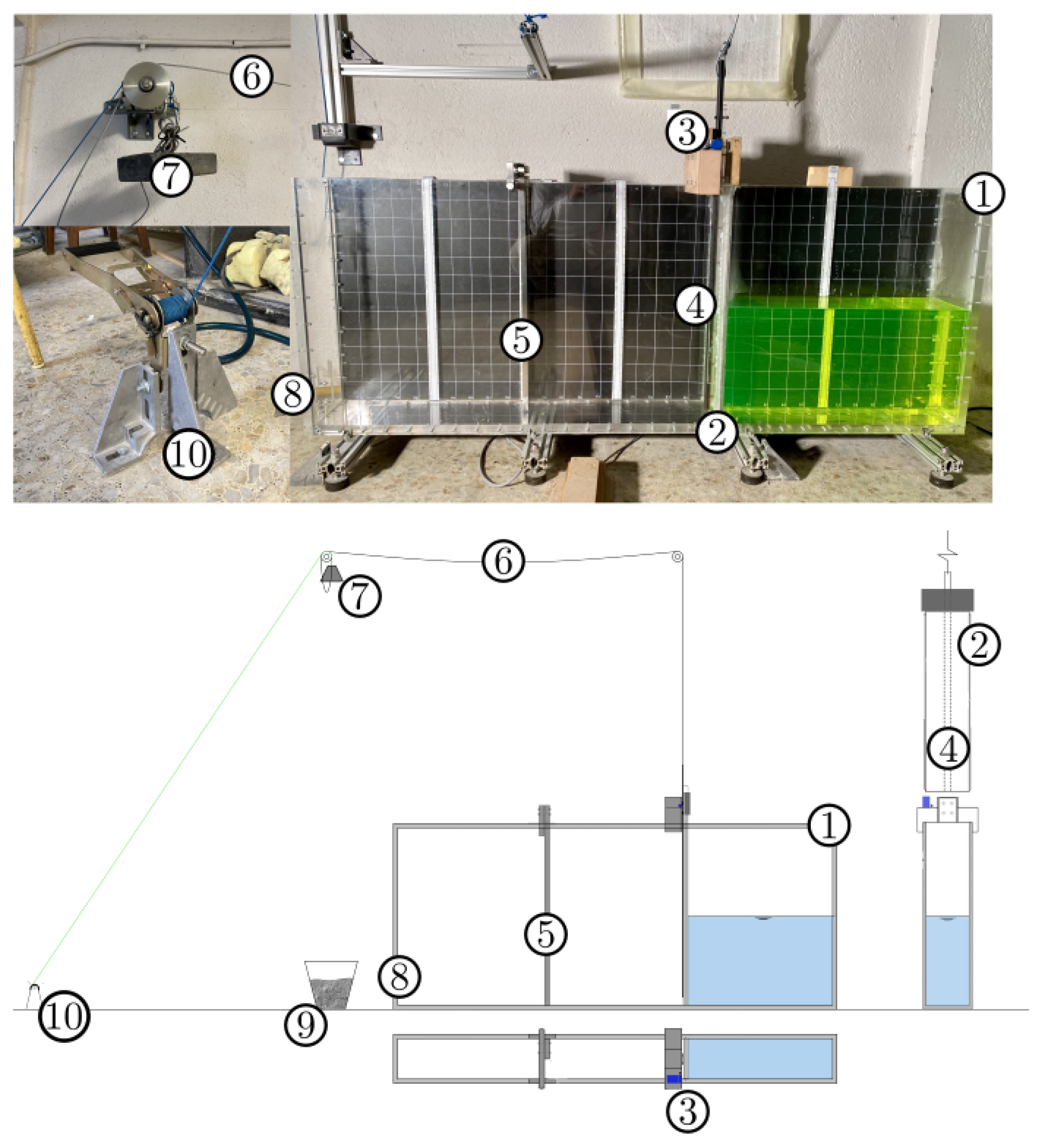
Figure 2.
Schematic of the tank with its dimensions (in mm) for the asymmetric flow configuration and the pressure probe locations. All distances are expressed in mm. Sensors 1, 2 and 3 record the pressure signals , and respectively.
Figure 2.
Schematic of the tank with its dimensions (in mm) for the asymmetric flow configuration and the pressure probe locations. All distances are expressed in mm. Sensors 1, 2 and 3 record the pressure signals , and respectively.
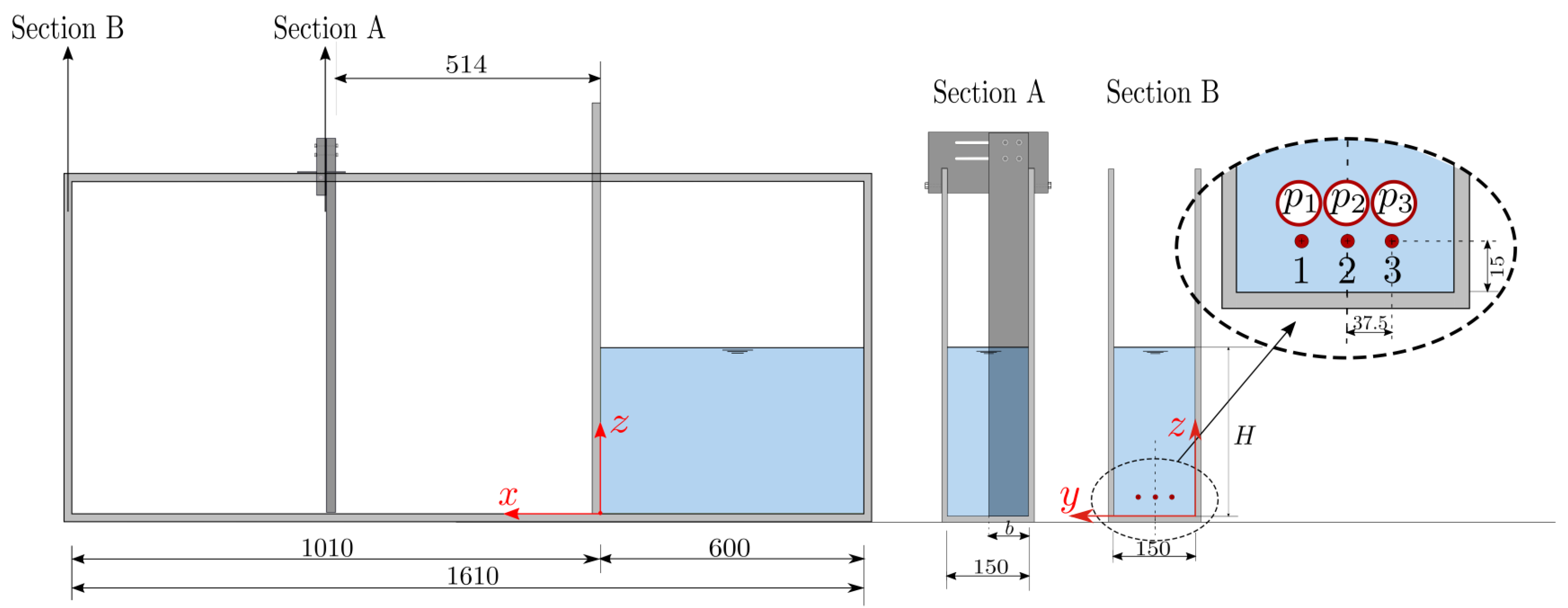
Figure 3.
Detail view of the CAD model of the obstacle placed in the asymmetric flow configuration diplaying the bracket and the plate. The length mm represents the width of the plate.
Figure 3.
Detail view of the CAD model of the obstacle placed in the asymmetric flow configuration diplaying the bracket and the plate. The length mm represents the width of the plate.
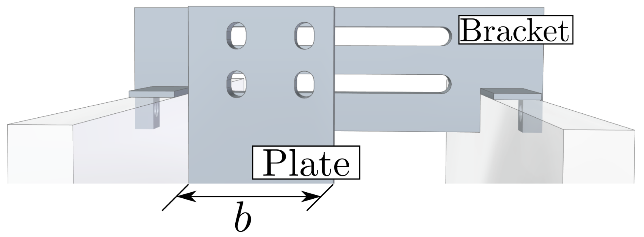
Figure 4.
Outline of the rise time and decay time definition. The continuous black line represents the triangular approximation of the pressure impulse.
Figure 4.
Outline of the rise time and decay time definition. The continuous black line represents the triangular approximation of the pressure impulse.
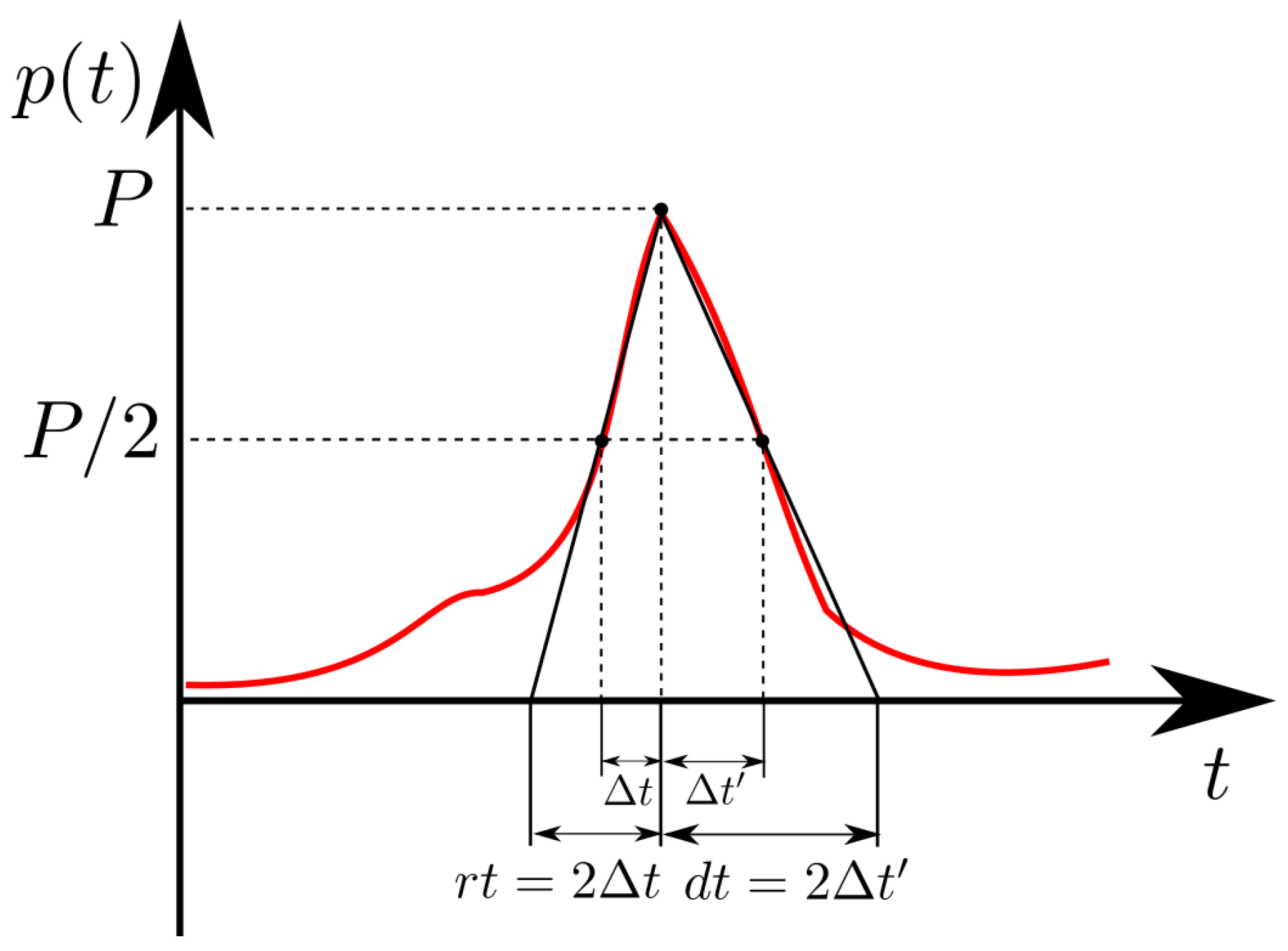
Figure 5.
Top view of the tested configurations: asymmetrical (left) and symmetrical (right). The breadth of the plate is b, the breadth of the inner volume of the tank is B, and the distance from the lateral wall to the center of the plate is y.
Figure 5.
Top view of the tested configurations: asymmetrical (left) and symmetrical (right). The breadth of the plate is b, the breadth of the inner volume of the tank is B, and the distance from the lateral wall to the center of the plate is y.
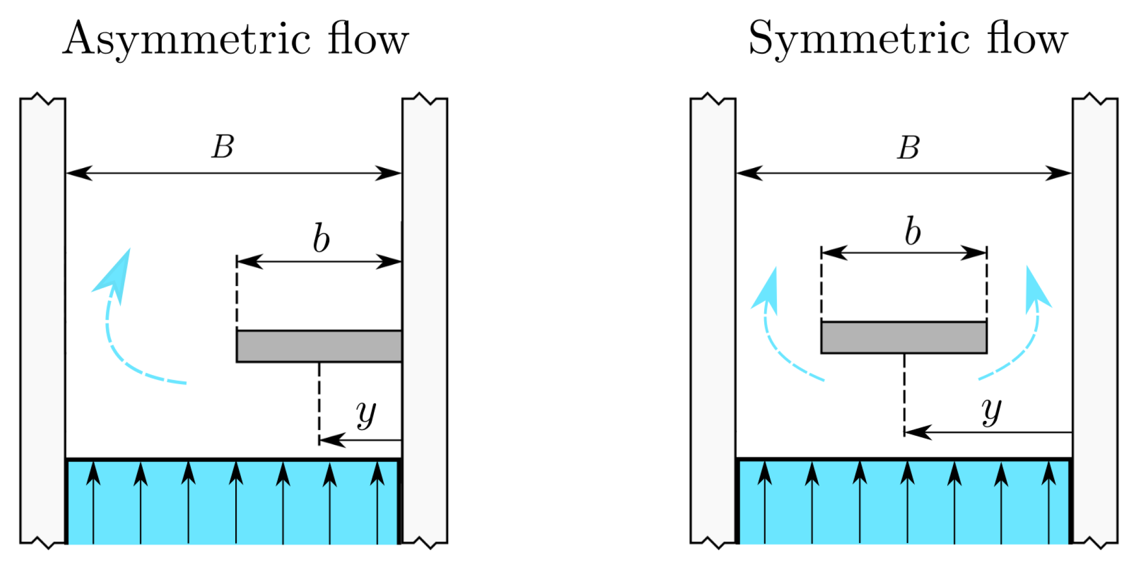
Figure 6.
Running mean (left) and running standard deviation (right) of the peak pressure values P for sensor 1 in non-dimensional units, dividing by . Presented values for asymmetric (continuous line) and symmetric configurations (dotted line).
Figure 6.
Running mean (left) and running standard deviation (right) of the peak pressure values P for sensor 1 in non-dimensional units, dividing by . Presented values for asymmetric (continuous line) and symmetric configurations (dotted line).
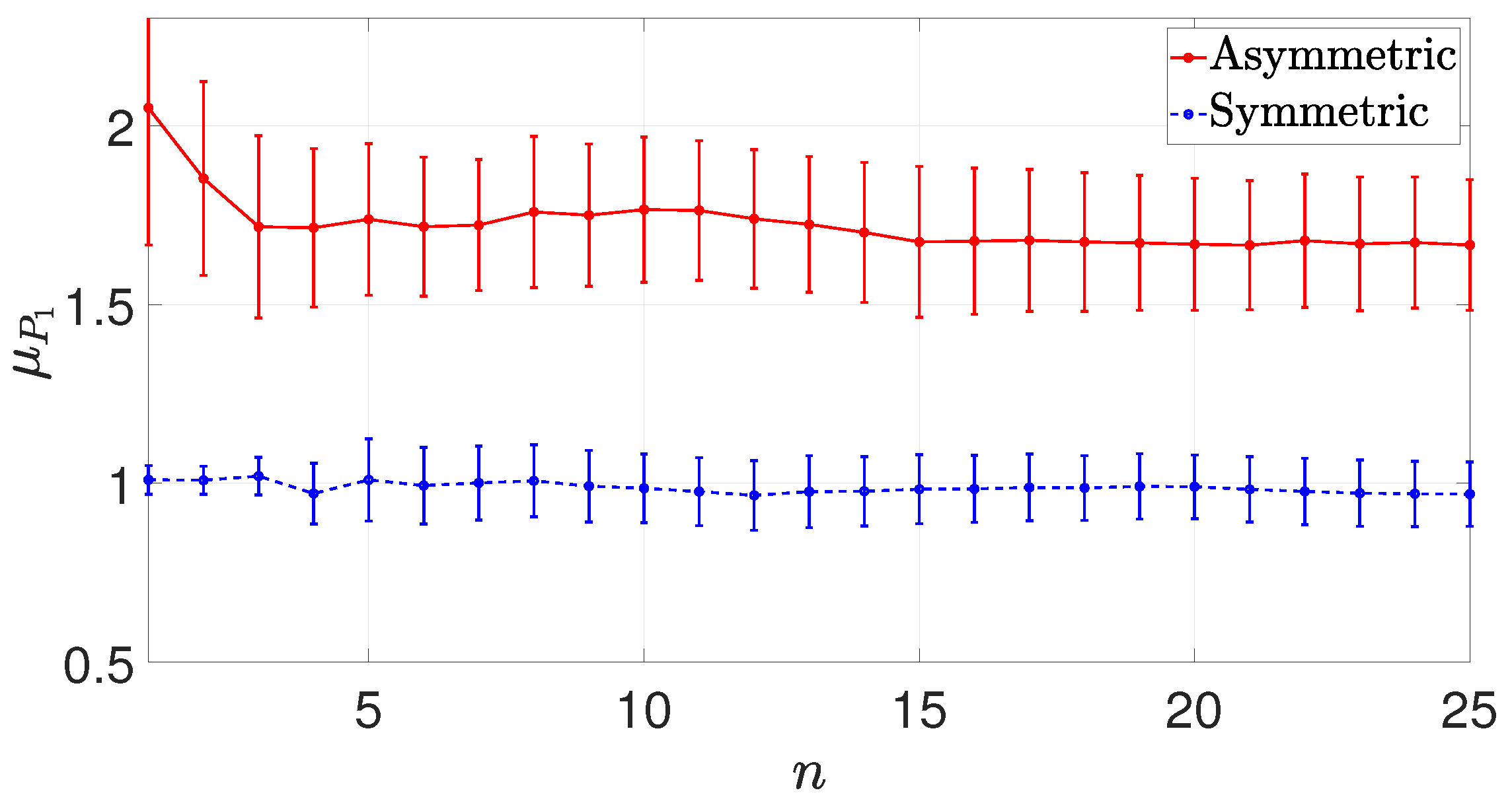
Figure 7.
Running mean (left) and running standard deviation (right) of the peak pressure values P for sensor 2 in non-dimensional units, dividing by . Presented values for asymmetric (continuous line) and symmetric configurations (dotted line).
Figure 7.
Running mean (left) and running standard deviation (right) of the peak pressure values P for sensor 2 in non-dimensional units, dividing by . Presented values for asymmetric (continuous line) and symmetric configurations (dotted line).
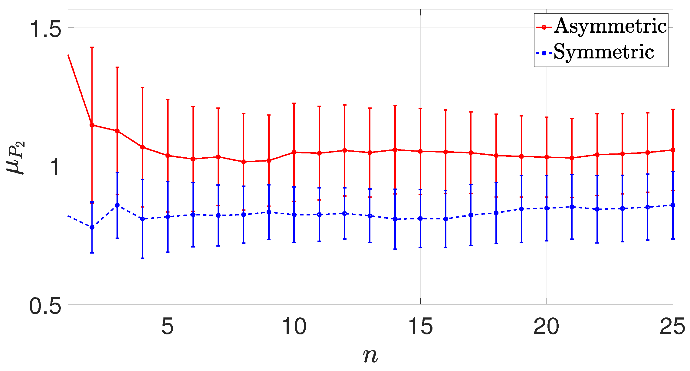
Figure 8.
Running mean (left) and running standard deviation (right) of the peak pressure values P for sensor 3 in non-dimensional units, dividing by . Presented values for asymmetric (continuous line) and symmetric configurations (dotted line).
Figure 8.
Running mean (left) and running standard deviation (right) of the peak pressure values P for sensor 3 in non-dimensional units, dividing by . Presented values for asymmetric (continuous line) and symmetric configurations (dotted line).
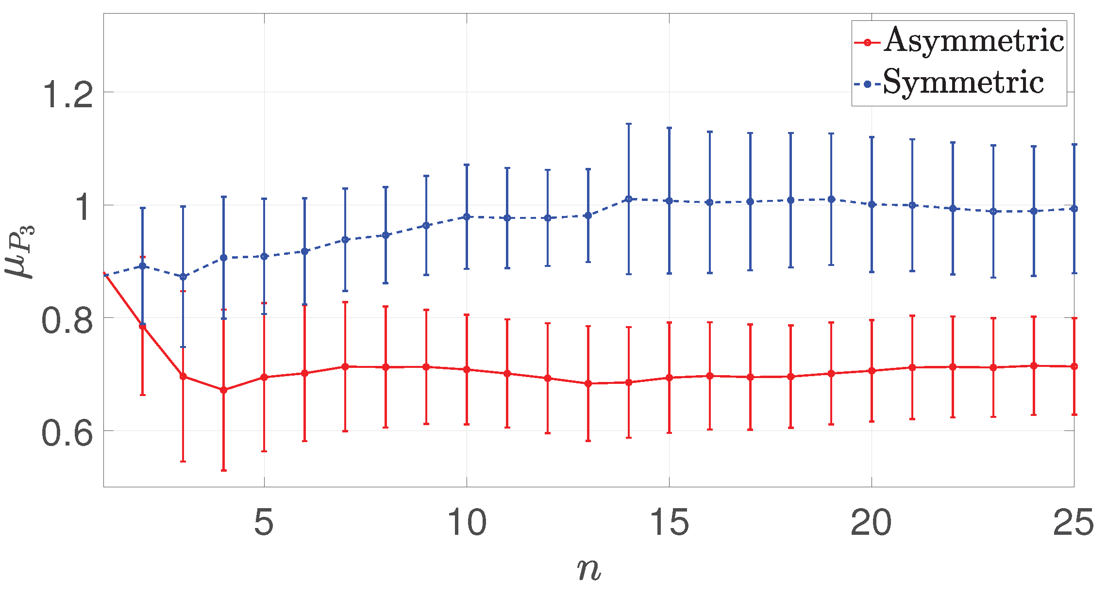
Figure 9.
Front view of the characteristic instants of a dam break experiment with the presence of an obstacle in the asymmetric configuration.
Figure 9.
Front view of the characteristic instants of a dam break experiment with the presence of an obstacle in the asymmetric configuration.
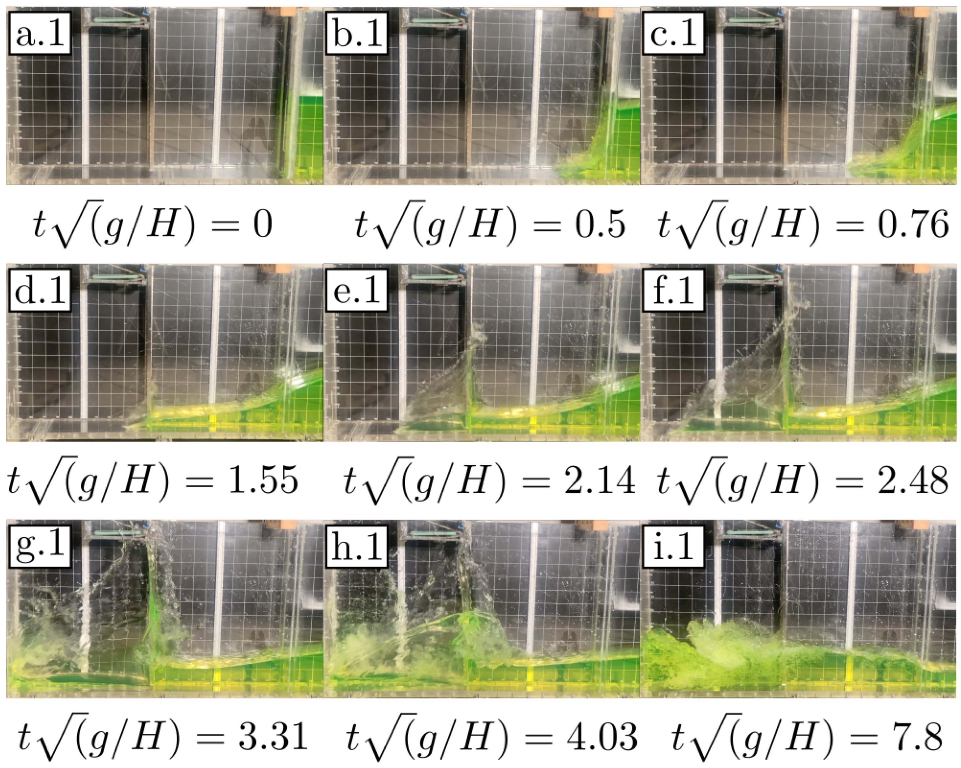
Figure 10.
Top view of the characteristic instants of a dam break experiment with the presence of an obstacle in the asymmetric configuration.
Figure 10.
Top view of the characteristic instants of a dam break experiment with the presence of an obstacle in the asymmetric configuration.
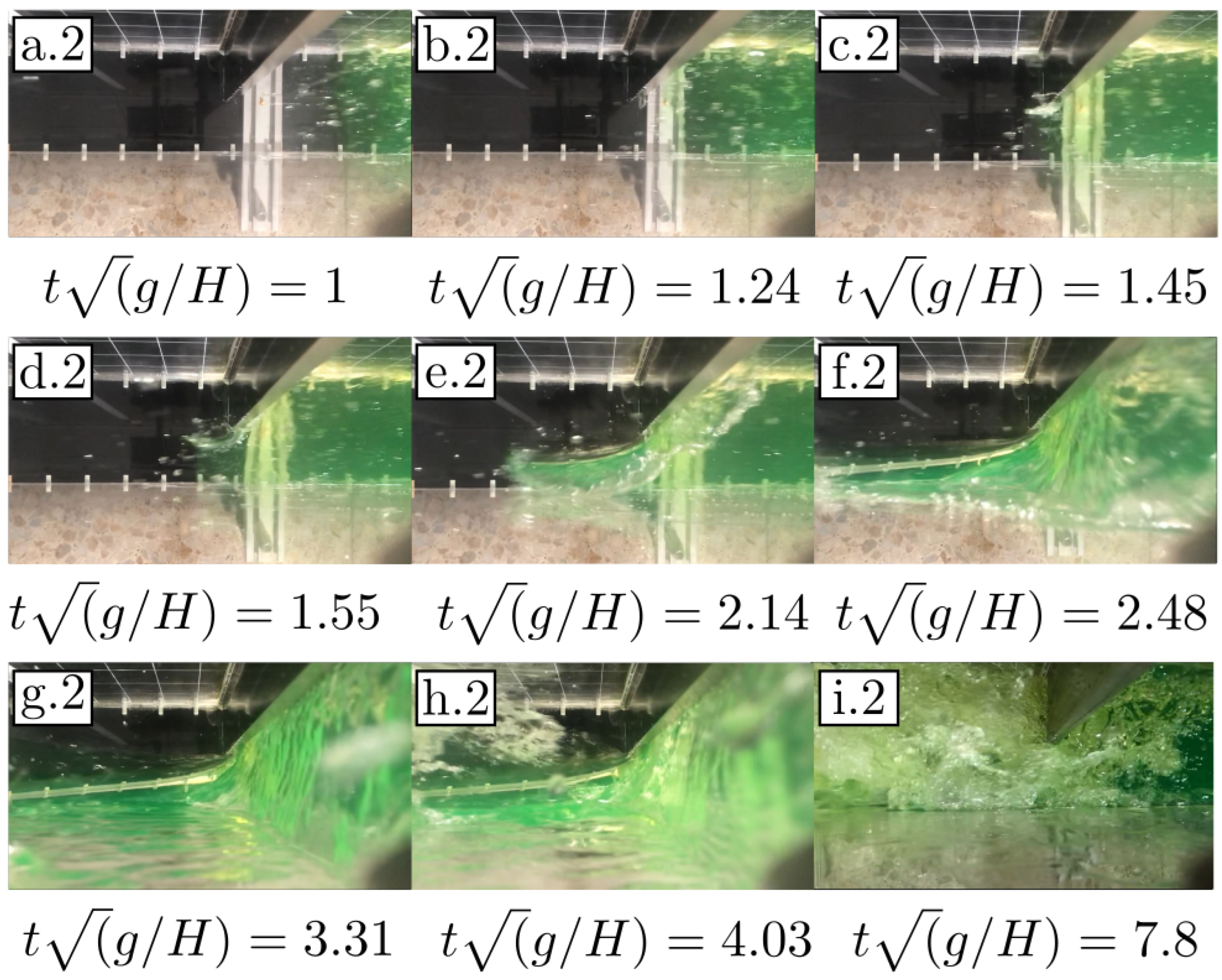
Figure 11.
Pressure measurements over time for sensors 1, 2 and 3 of a typical impact event in the asymmetric configuration.
Figure 11.
Pressure measurements over time for sensors 1, 2 and 3 of a typical impact event in the asymmetric configuration.
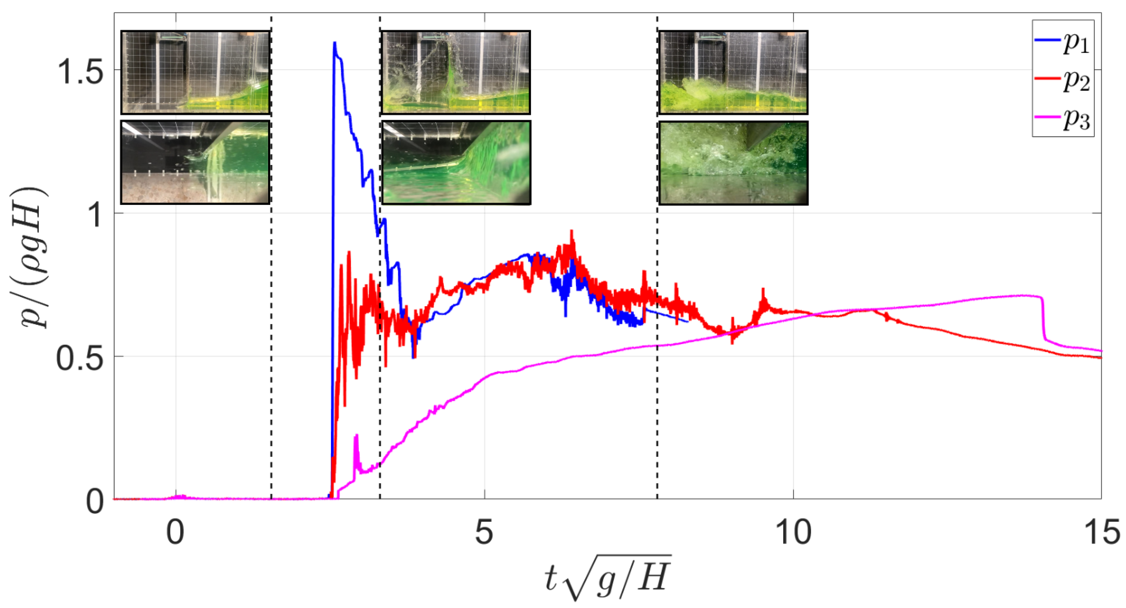
Figure 12.
Sensor 1 pressure time histories for the 25 repetitions in the asymmetric flow configuration. The central black dotted line indicates de median, the upper and lower black dotted lines indicate the 97.5 % and 2.5 % percentiles respectively.
Figure 12.
Sensor 1 pressure time histories for the 25 repetitions in the asymmetric flow configuration. The central black dotted line indicates de median, the upper and lower black dotted lines indicate the 97.5 % and 2.5 % percentiles respectively.
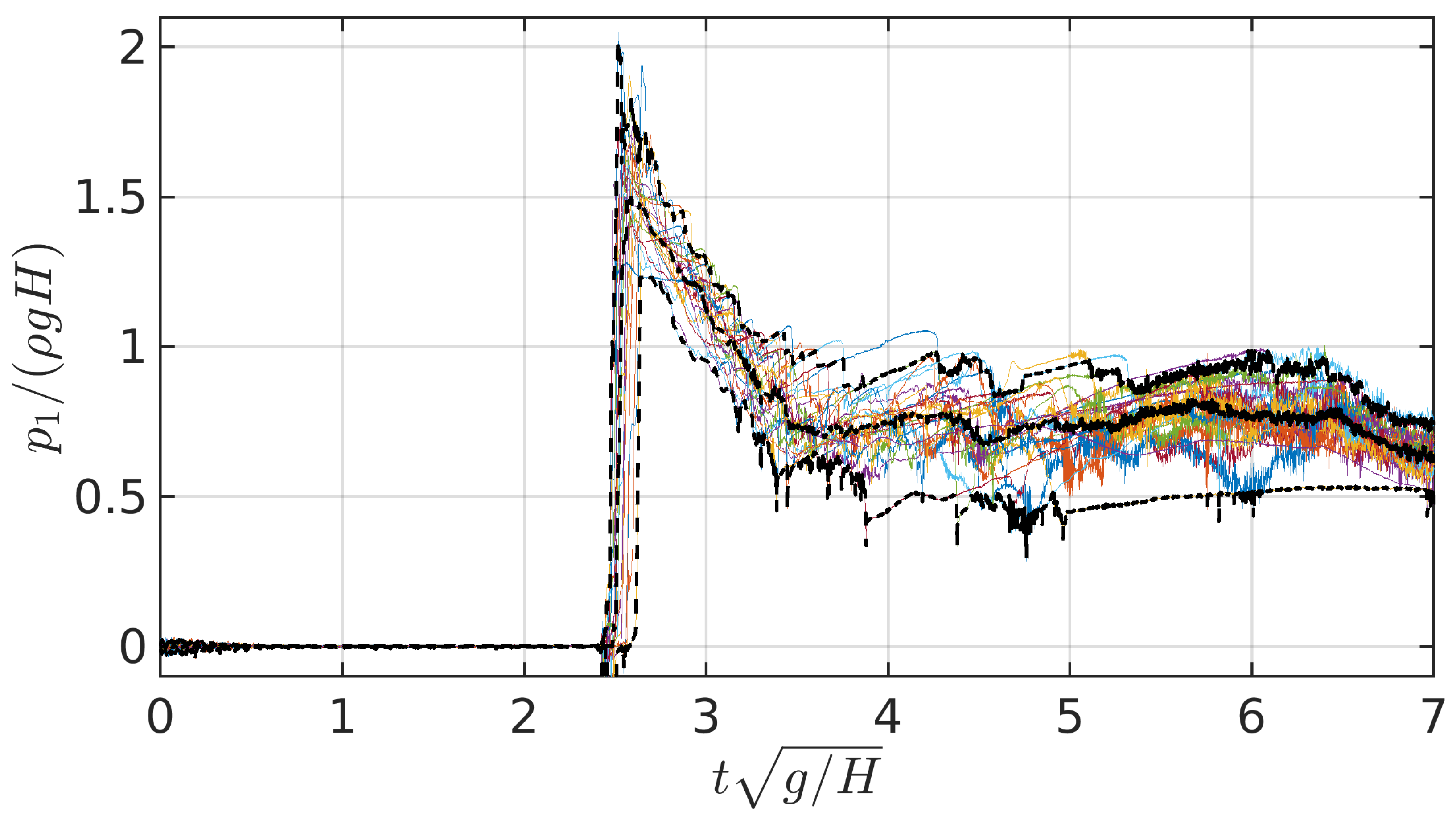
Figure 13.
Sensor 2 pressure time histories for the 25 repetitions in the asymmetric flow configuration. The central black dotted line indicates de median, the upper and lower black dotted lines indicate the 97.5 % and 2.5 % percentiles respectively.
Figure 13.
Sensor 2 pressure time histories for the 25 repetitions in the asymmetric flow configuration. The central black dotted line indicates de median, the upper and lower black dotted lines indicate the 97.5 % and 2.5 % percentiles respectively.
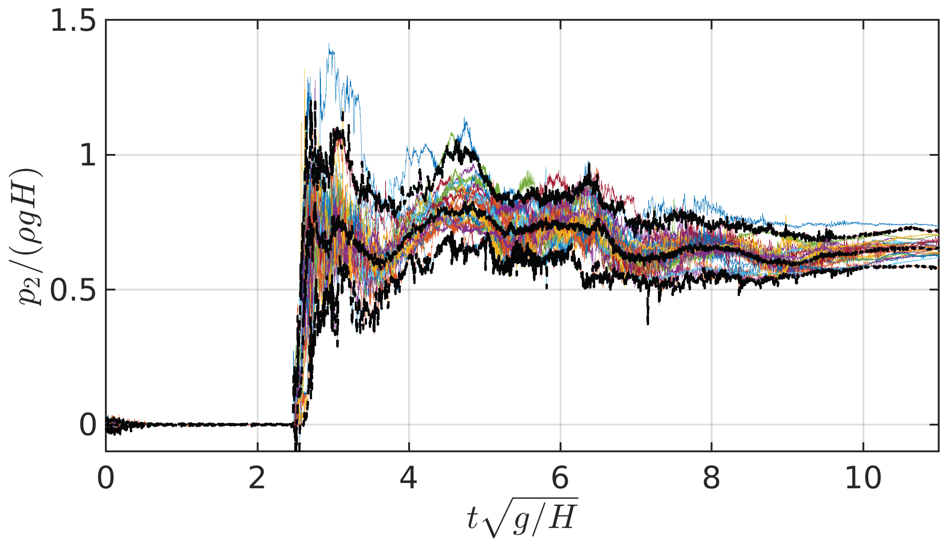
Figure 14.
Sensor 3 pressure time histories for the 25 repetitions in the asymmetric flow configuration. The central black dotted line indicates de median, the upper and lower black dotted lines indicate the 97.5 % and 2.5 % percentiles respectively.
Figure 14.
Sensor 3 pressure time histories for the 25 repetitions in the asymmetric flow configuration. The central black dotted line indicates de median, the upper and lower black dotted lines indicate the 97.5 % and 2.5 % percentiles respectively.
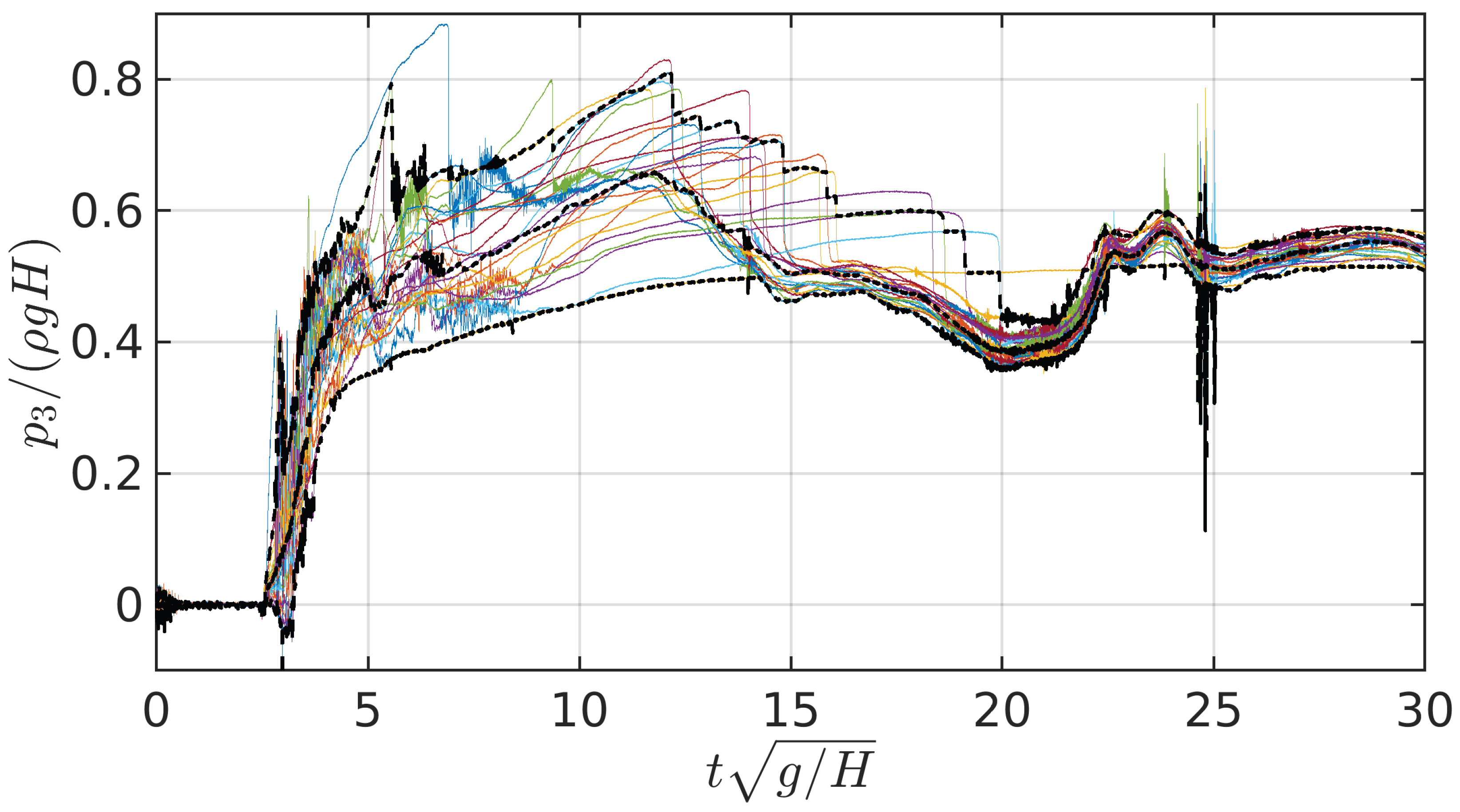
Figure 15.
ECDF of the pressure peak P for sensors 1, 2 and 3 in the asymmetric configuration.
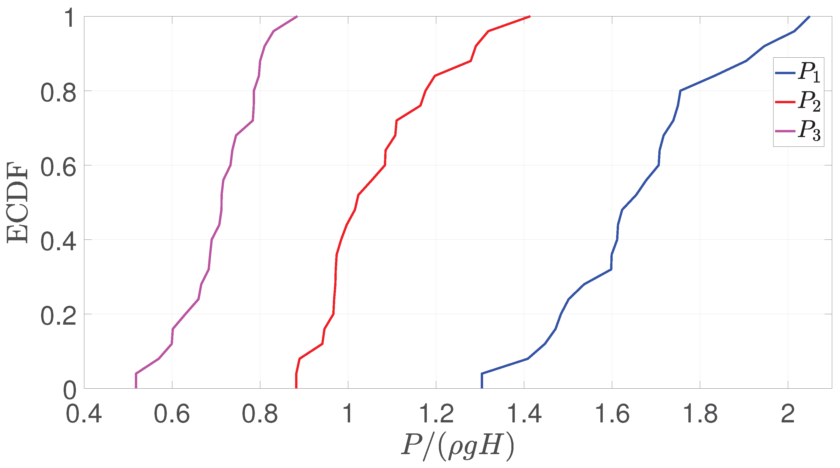
Figure 16.
Maximum pressure peaks of sensors 1, 2 and 3 and their repective medians for the conducted 25 tests in the asymmetric flow configuration.
Figure 16.
Maximum pressure peaks of sensors 1, 2 and 3 and their repective medians for the conducted 25 tests in the asymmetric flow configuration.
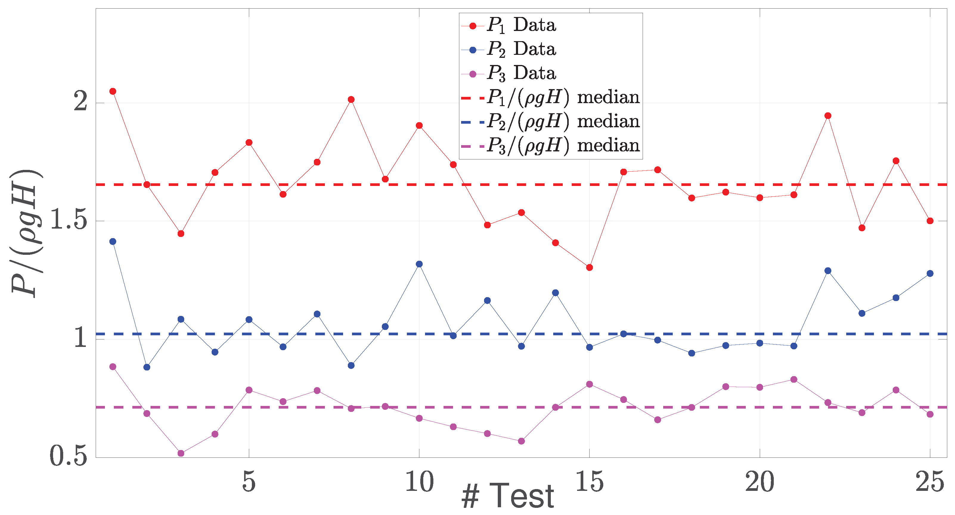
Figure 17.
Maximum pressure peak instants of sensors 1, 2 and 3 and their repective medians for the conducted 25 tests in the asymmetric flow configuration.
Figure 17.
Maximum pressure peak instants of sensors 1, 2 and 3 and their repective medians for the conducted 25 tests in the asymmetric flow configuration.
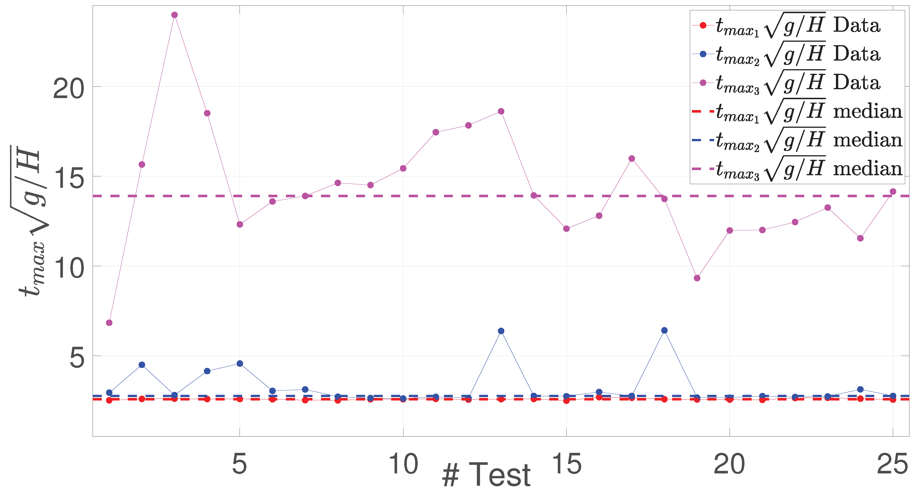
Figure 18.
Correlation between maximum pressure peak recorded by sensor 1 () and sensors 2 and 3 ( and ). Mean values are expressed by the red dotted lines. The black dotted line represents the linear fitting to the data. The 25%, 50% and 75% probability regions of the bivariate normal distribution of the sample has been plotted as reference.
Figure 19.
Correlation between the rise time () and maximum pressure peak (P) of sensors 1 and 3. Mean values are expressed by the red dotted lines. The black dotted line represents the linear fitting to the data. The 25%, 50% and 75% probability regions of the bivariate normal distribution of the sample has been plotted as reference.
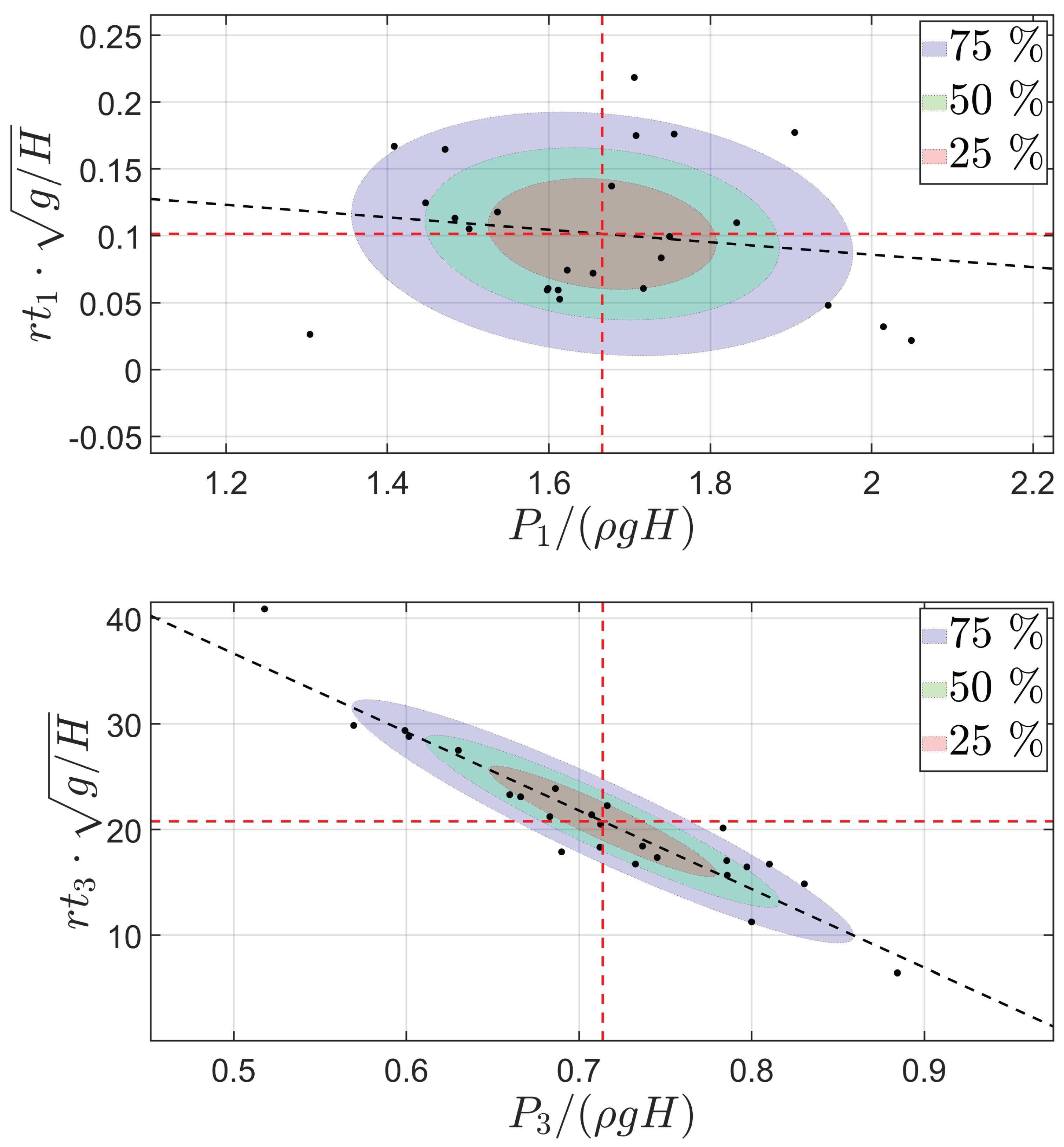
Figure 20.
ECDF of the rise and decay times for sensor 1 in the asymmetric configuration.
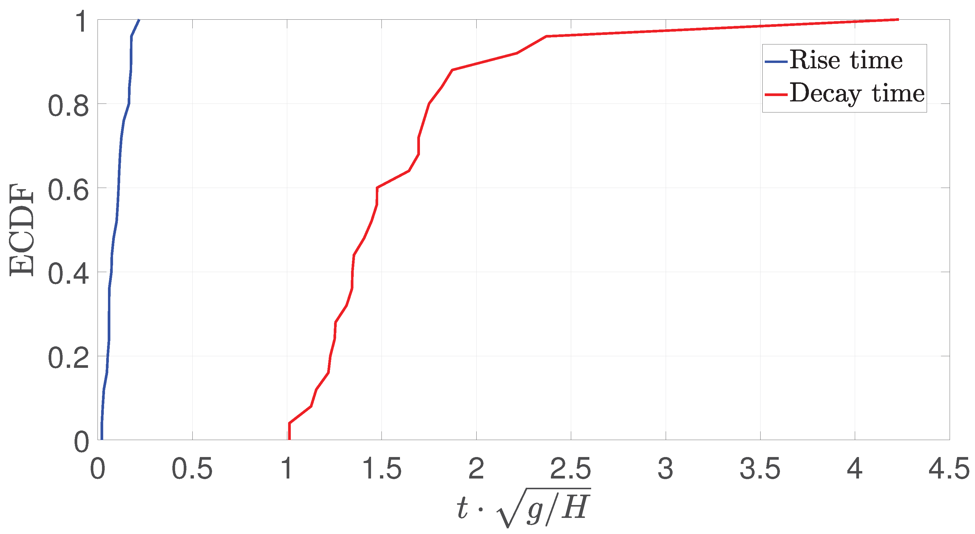
Figure 21.
ECDF of the pressure impulse (I) calculated from the pressure signals recorder by sensor 1. The red line represents the impulse calculated using the triangular approximation.
Figure 21.
ECDF of the pressure impulse (I) calculated from the pressure signals recorder by sensor 1. The red line represents the impulse calculated using the triangular approximation.
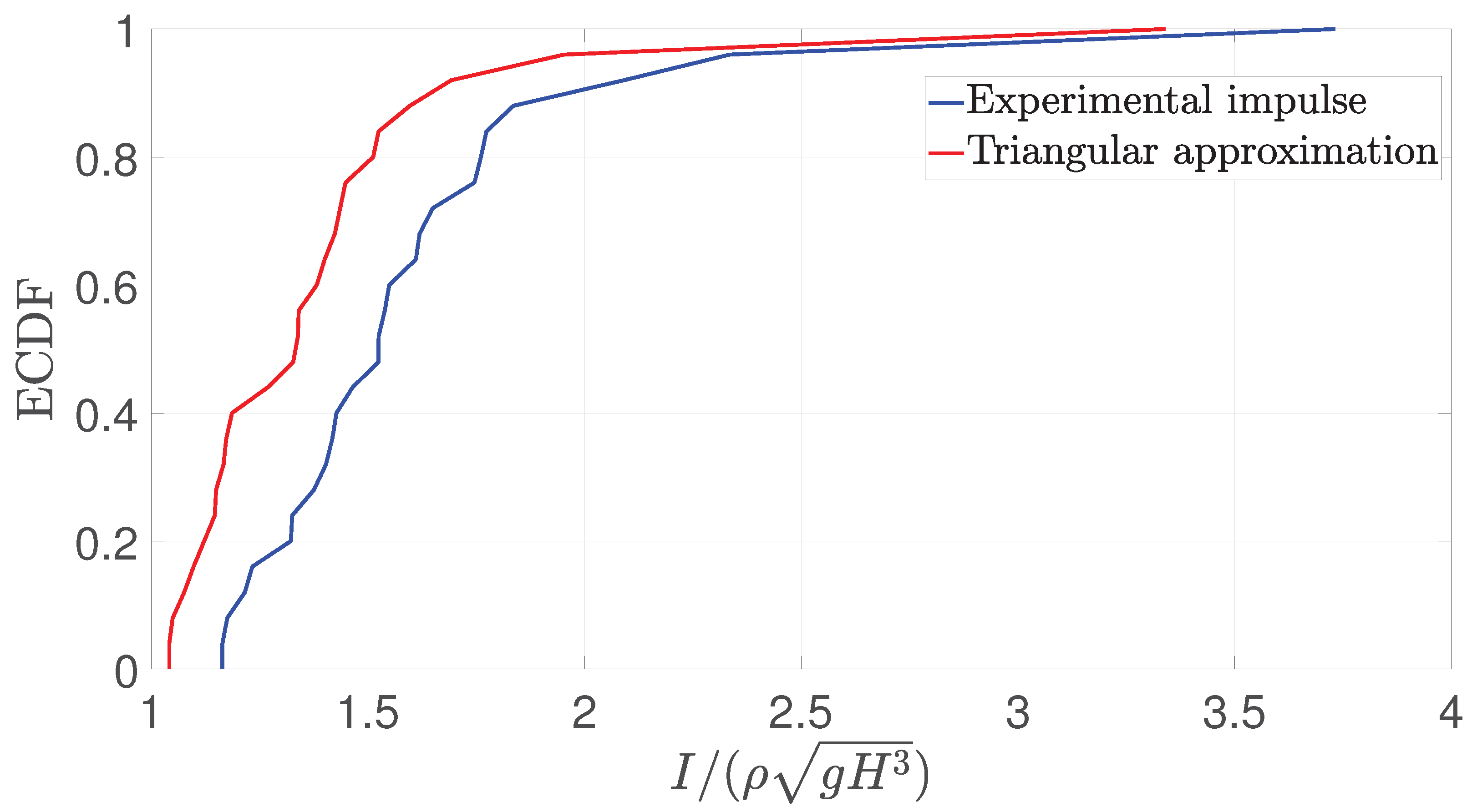
Figure 22.
Front view of the characteristic instants of a dam break experiment with the presence of an obstacle in the symmetric configuration.
Figure 22.
Front view of the characteristic instants of a dam break experiment with the presence of an obstacle in the symmetric configuration.
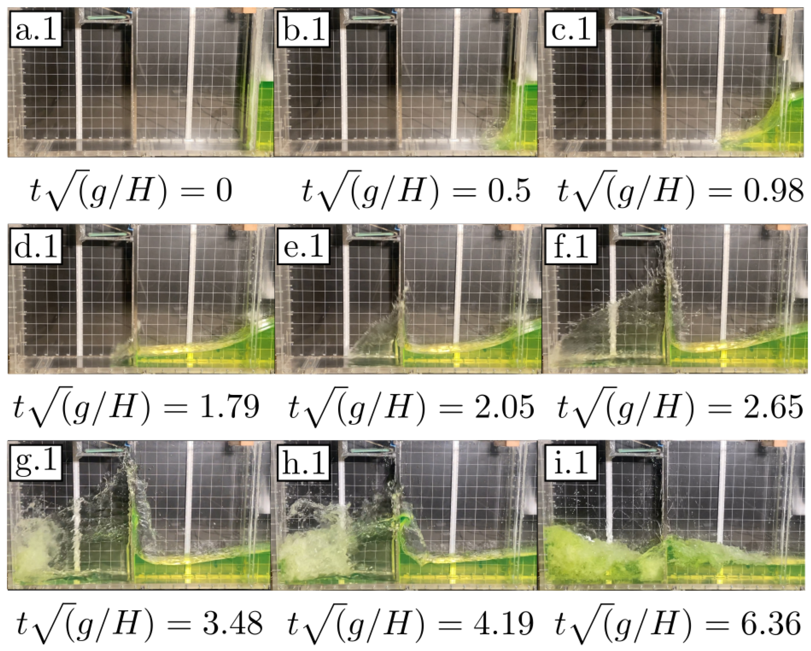
Figure 23.
Top view of the characteristic instants of a dam break experiment in the presence of an obstacle, symmetric configuration.
Figure 23.
Top view of the characteristic instants of a dam break experiment in the presence of an obstacle, symmetric configuration.
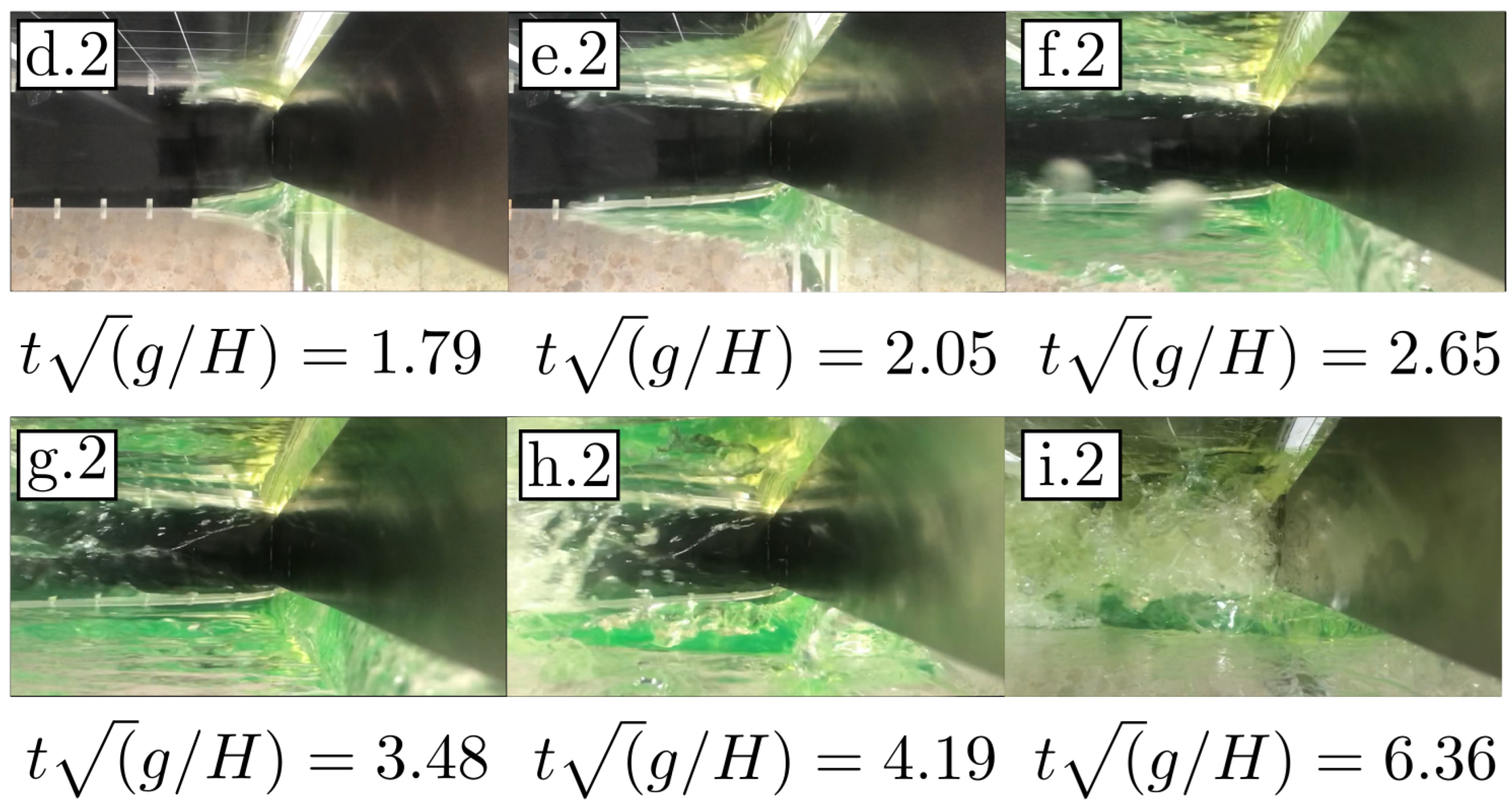
Figure 24.
Pressure measurements over time for sensors 1, 2 and 3 of a typical impact event in the symmetric configuration.
Figure 24.
Pressure measurements over time for sensors 1, 2 and 3 of a typical impact event in the symmetric configuration.
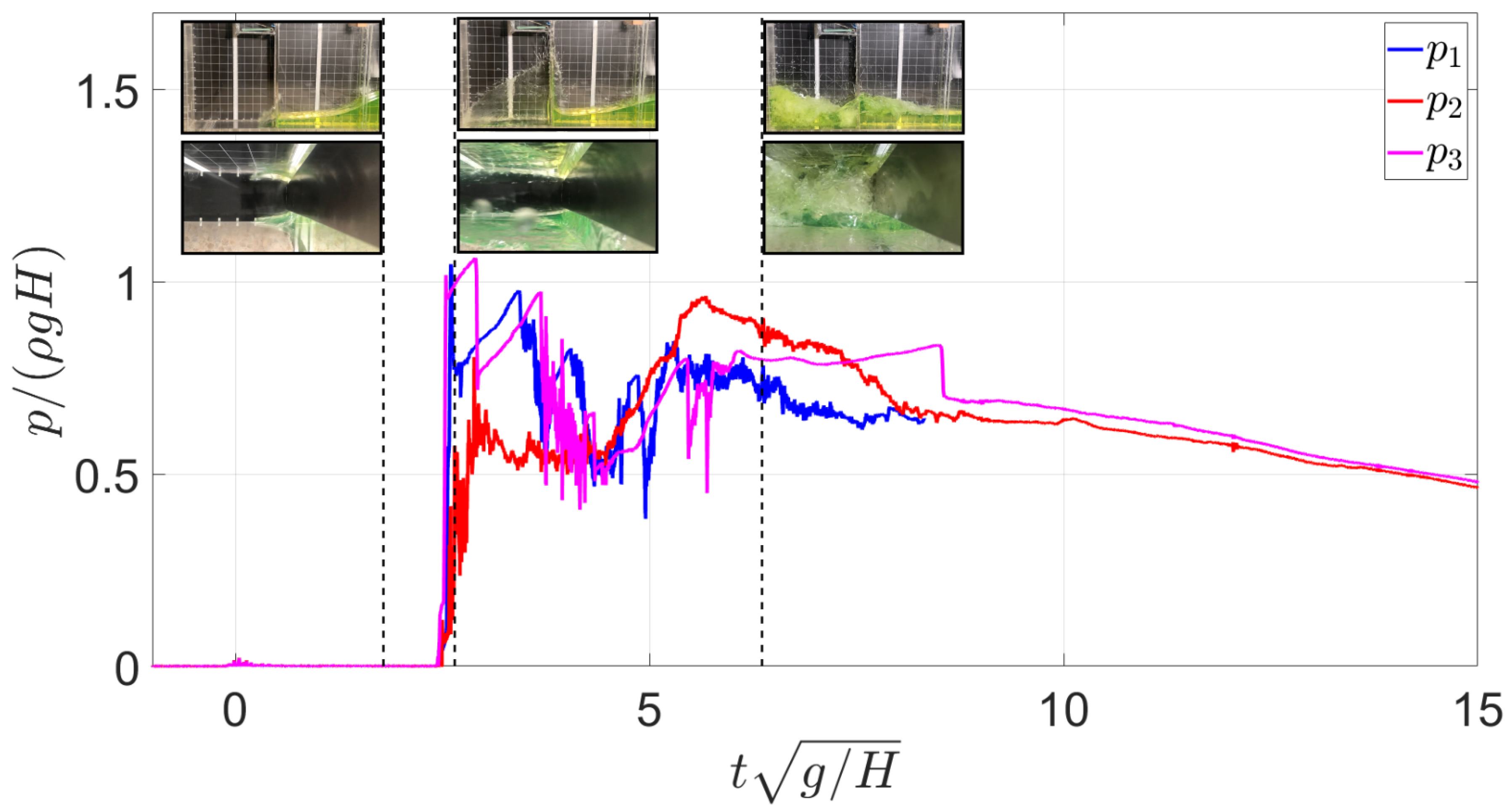
Figure 25.
Sensor 1 pressure time histories for the 25 repetitions in the symmetric flow configuration. The central black dotted line indicates de median, the upper and lower black dotted lines indicate the 97.5 % and 2.5 % percentiles respectively.
Figure 25.
Sensor 1 pressure time histories for the 25 repetitions in the symmetric flow configuration. The central black dotted line indicates de median, the upper and lower black dotted lines indicate the 97.5 % and 2.5 % percentiles respectively.
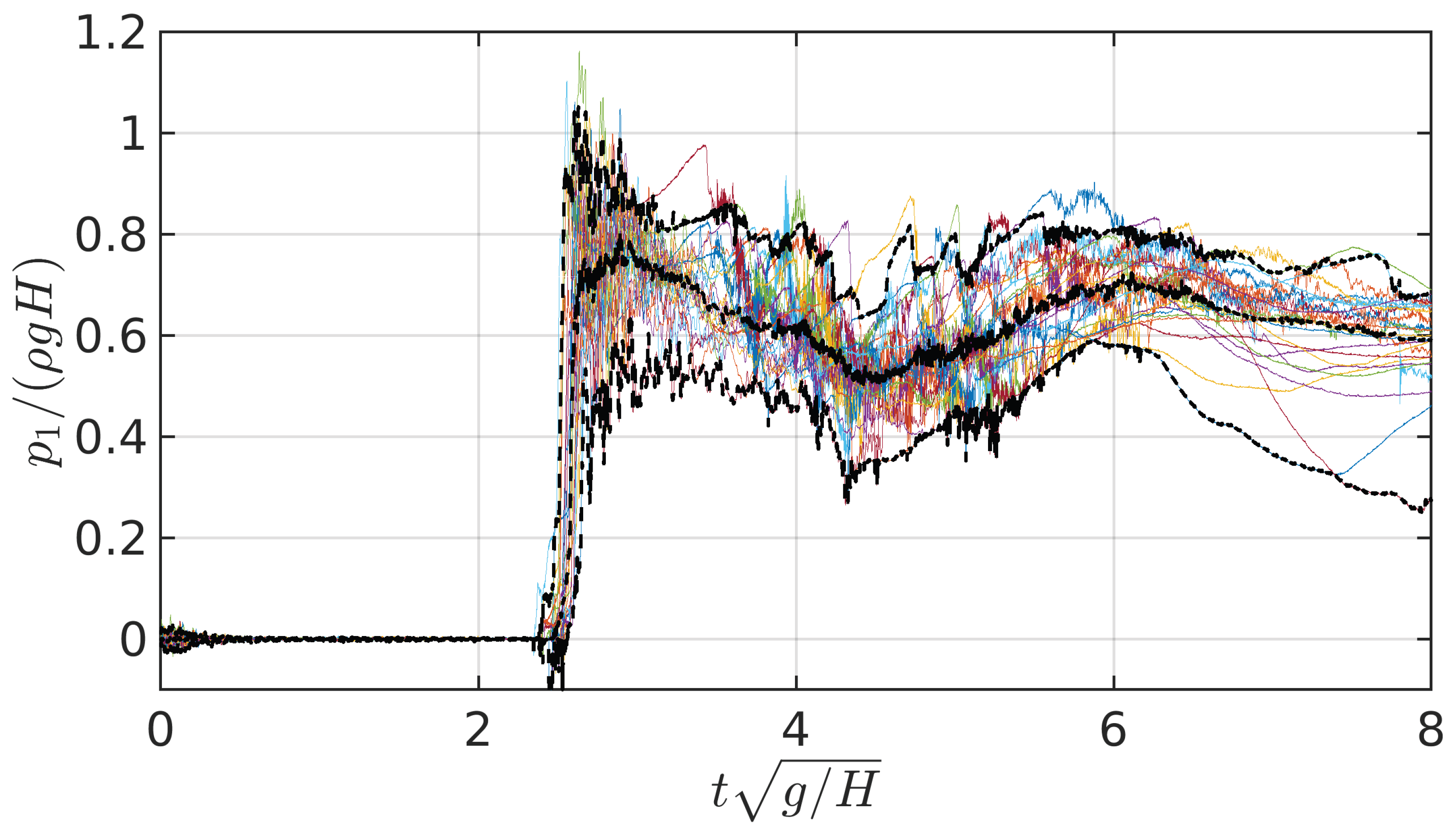
Figure 26.
Sensor 2 pressure time histories for the 25 repetitions in the symmetric flow configuration. The central black dotted line indicates de median, the upper and lower black dotted lines indicate the 97.5 % and 2.5 % percentiles respectively.
Figure 26.
Sensor 2 pressure time histories for the 25 repetitions in the symmetric flow configuration. The central black dotted line indicates de median, the upper and lower black dotted lines indicate the 97.5 % and 2.5 % percentiles respectively.
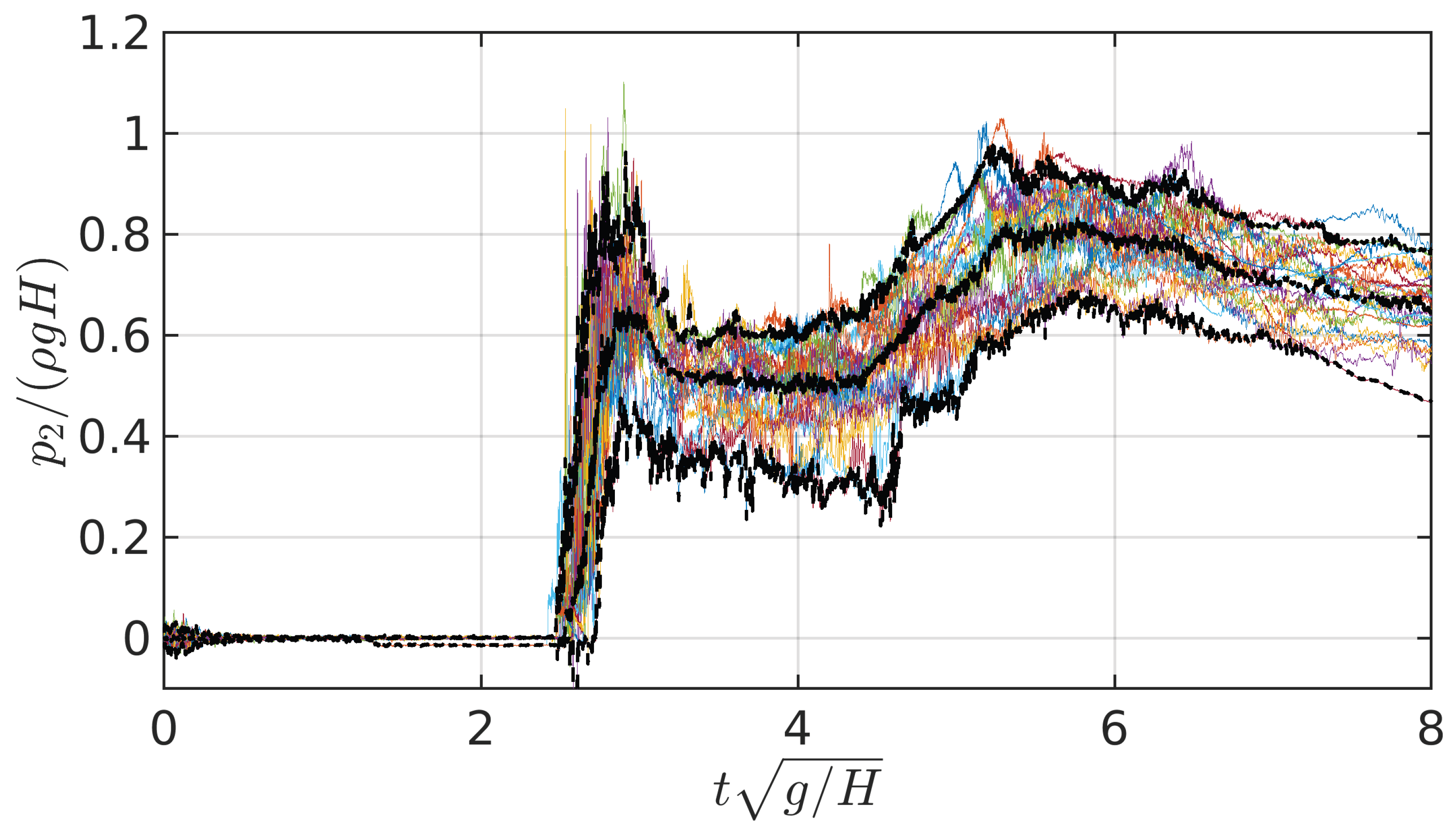
Figure 27.
Sensor 3 pressure time histories for the 25 repetitions in the symmetric flow configuration. The central black dotted line indicates de median, the upper and lower black dotted lines indicate the 97.5 % and 2.5 % percentiles respectively.
Figure 27.
Sensor 3 pressure time histories for the 25 repetitions in the symmetric flow configuration. The central black dotted line indicates de median, the upper and lower black dotted lines indicate the 97.5 % and 2.5 % percentiles respectively.
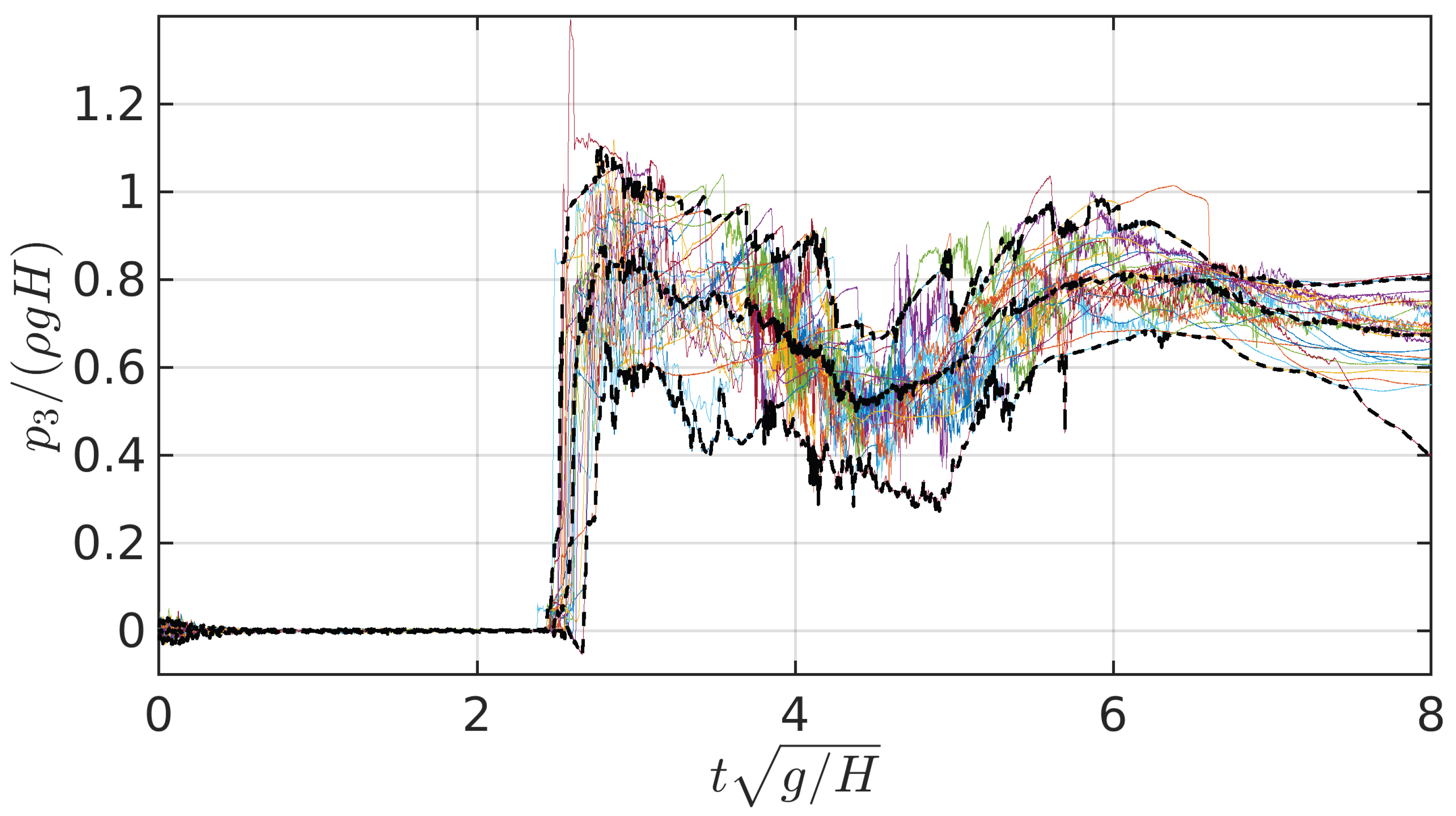
Figure 28.
Up: ECDF of the pressure peak P for sensors 1, 2 and 3 in the symmetric configuration. The 95% confidence intervals have been plotted in dotted color lines for sensors 1 and 3. The black dotted line represents the fitted sigmoid function to the data of sensors 1 and 3. Down: CDF of the normalized pressure peaks from sensors 1 and 3 along with the 95 % confidence intervals and the Standard normal CDF.
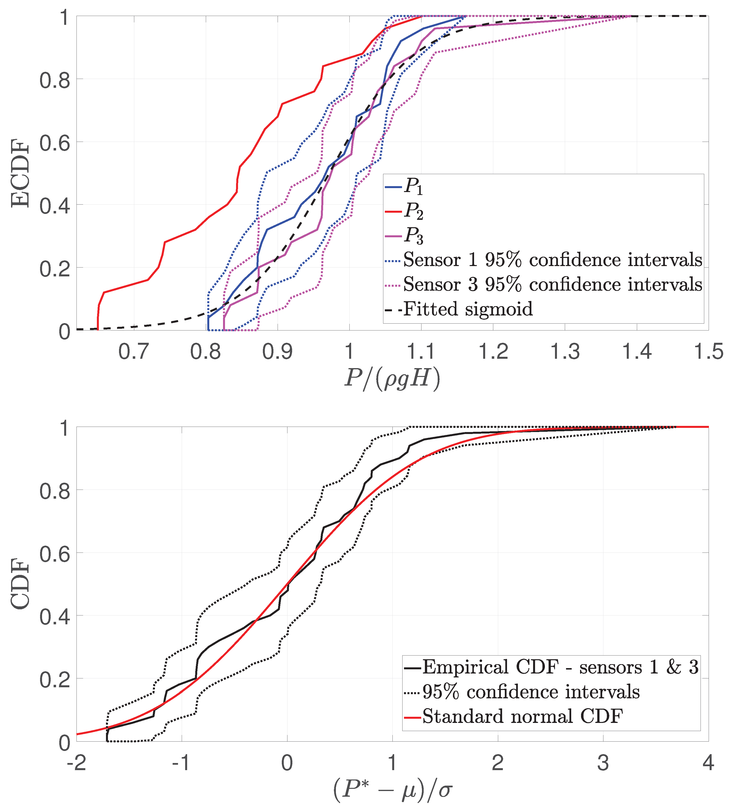
Figure 29.
Maximum pressure peaks of sensors 1, 2 and 3 and their repective medians for the conducted 25 tests in the symmetric flow configuration.
Figure 29.
Maximum pressure peaks of sensors 1, 2 and 3 and their repective medians for the conducted 25 tests in the symmetric flow configuration.
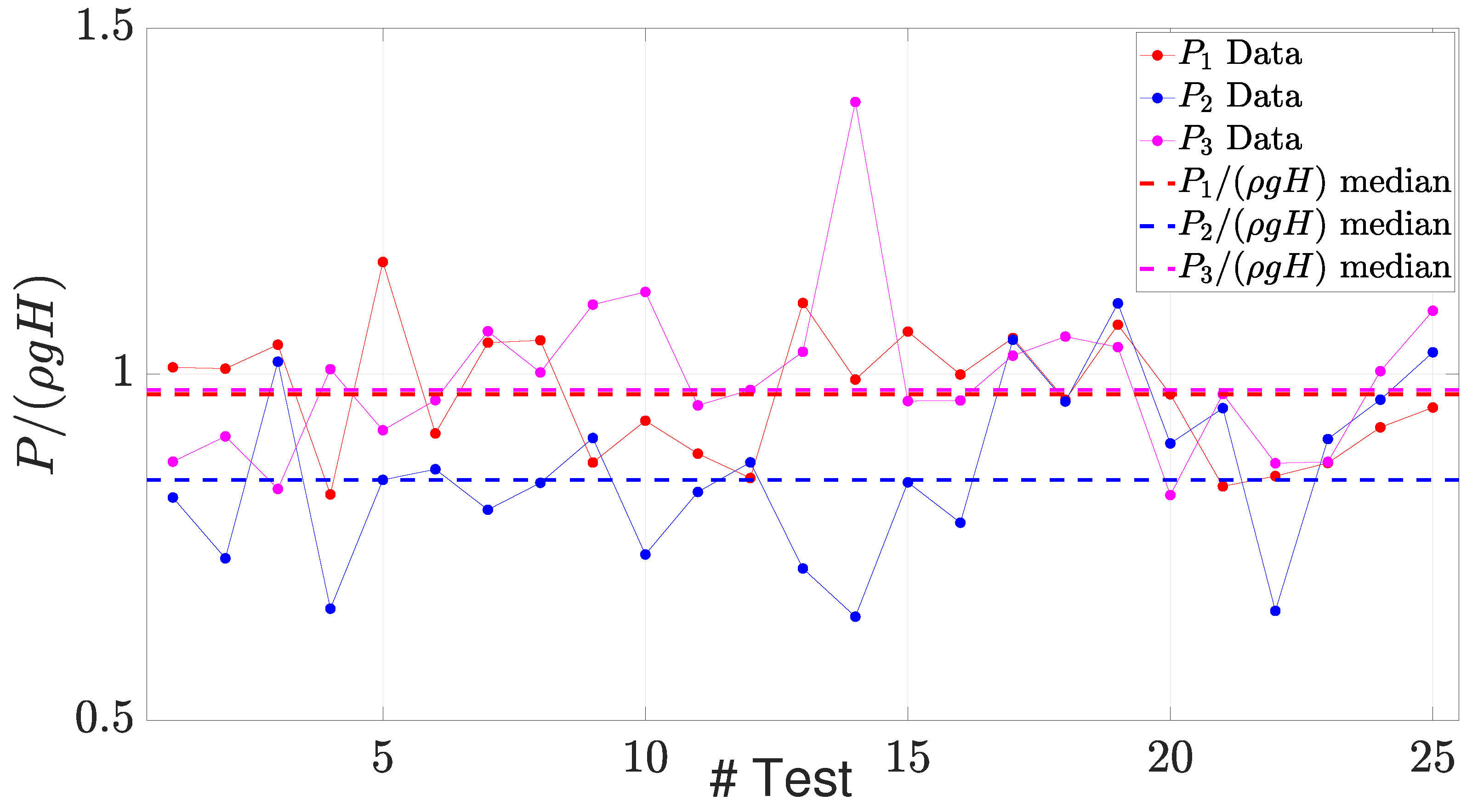
Figure 30.
Maximum pressure peak instants of sensors 1, 2 and 3 and their repective medians for the conducted 25 tests in the symmetric flow configuration.
Figure 30.
Maximum pressure peak instants of sensors 1, 2 and 3 and their repective medians for the conducted 25 tests in the symmetric flow configuration.
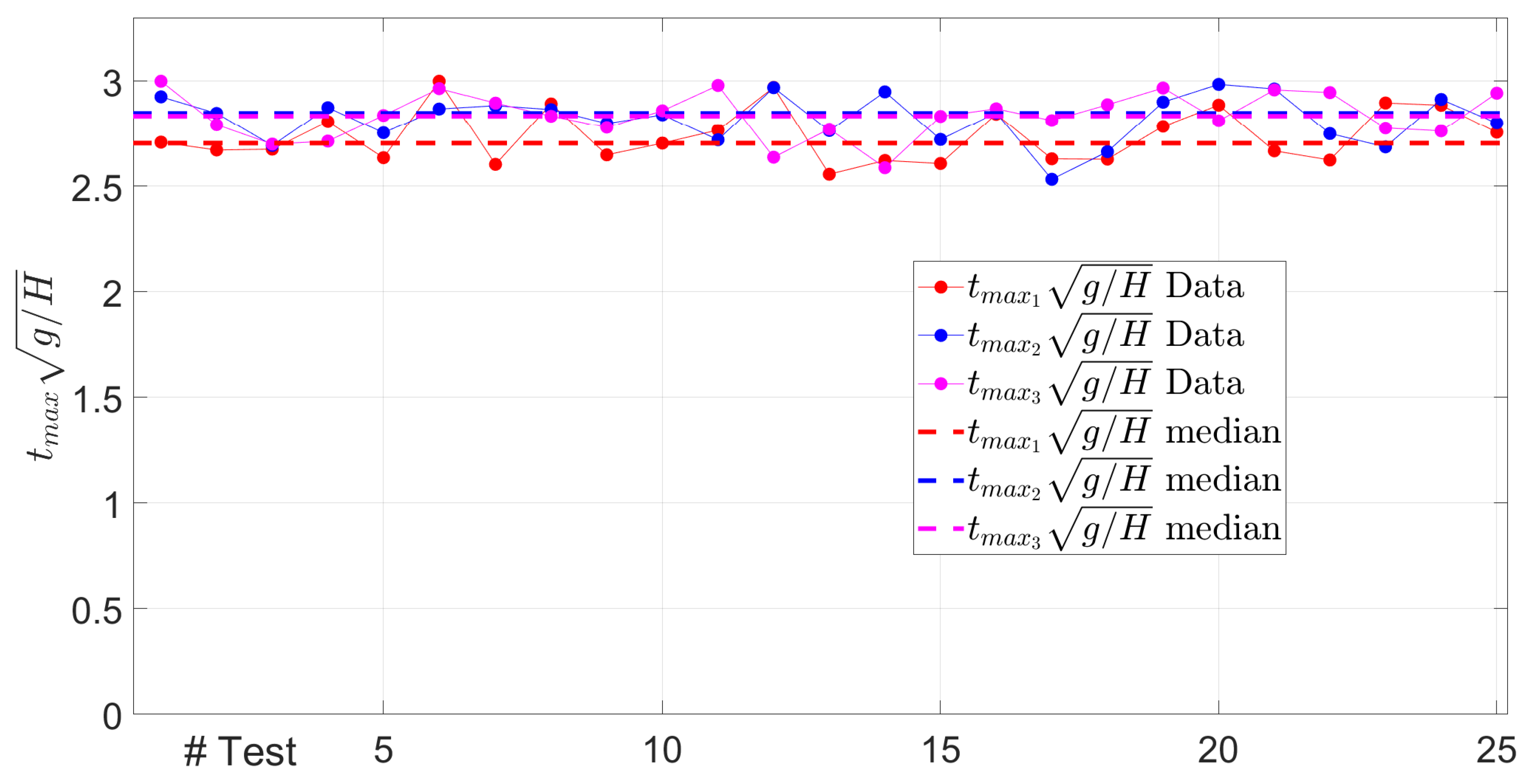
Figure 31.
Correlation between the maximum pressure peaks recorded by sensor 1 () and sensor 3 ().Mean values are expressed by the red dotted lines. The black dotted line represents the linear fitting to the data. The 25%, 50% and 75% probability regions of the bivariate normal distribution of the sample has been plotted as reference.
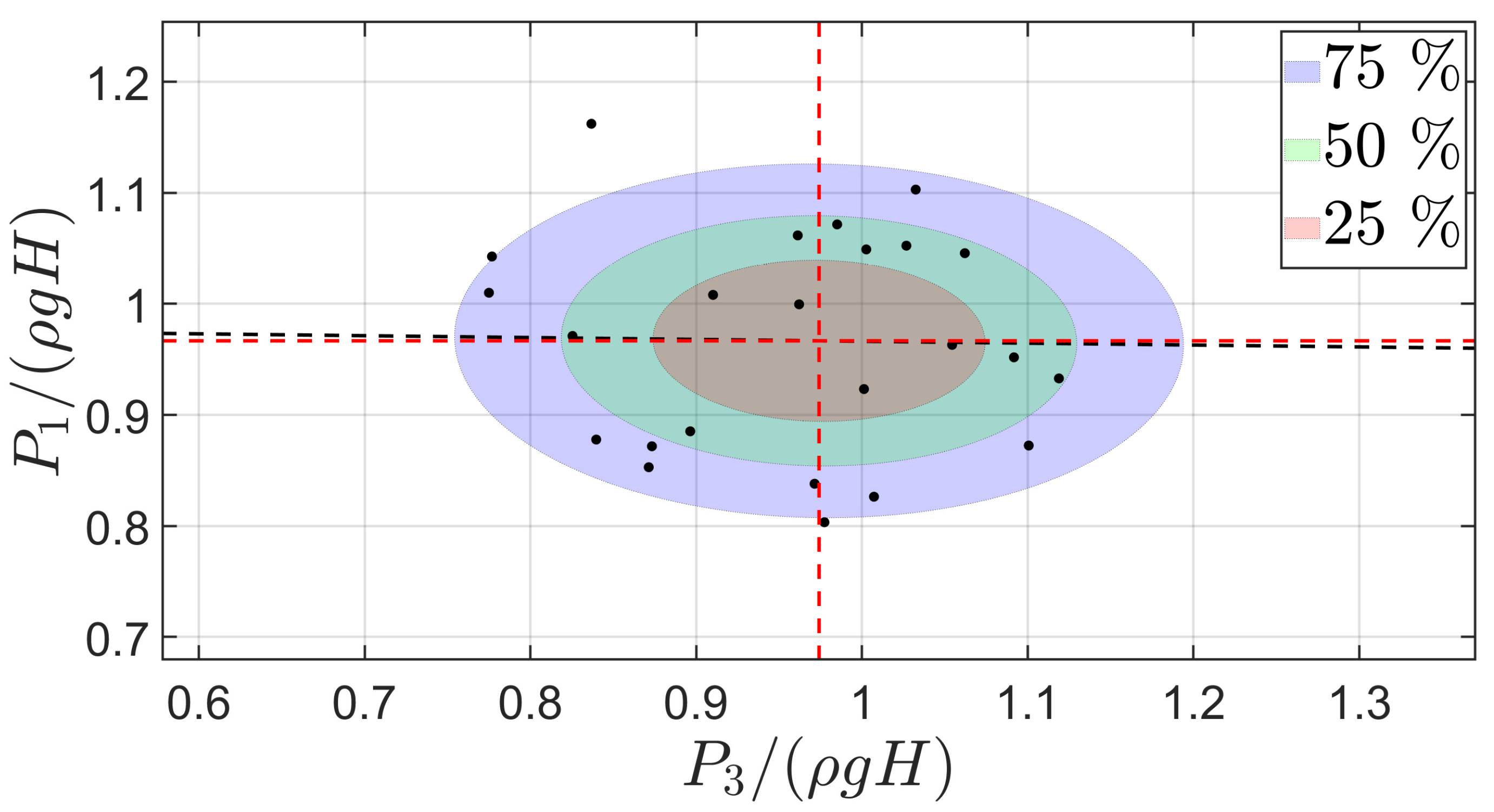
Figure 32.
Correlation between the rise time () and maximum pressure peak (P) of sensors 1, 2 and 3. Mean values are expressed by the red dotted lines. The black dotted line represents the linear fitting to the data. The 25%, 50% and 75% probability regions of the bivariate normal distribution of the sample has been plotted as reference.
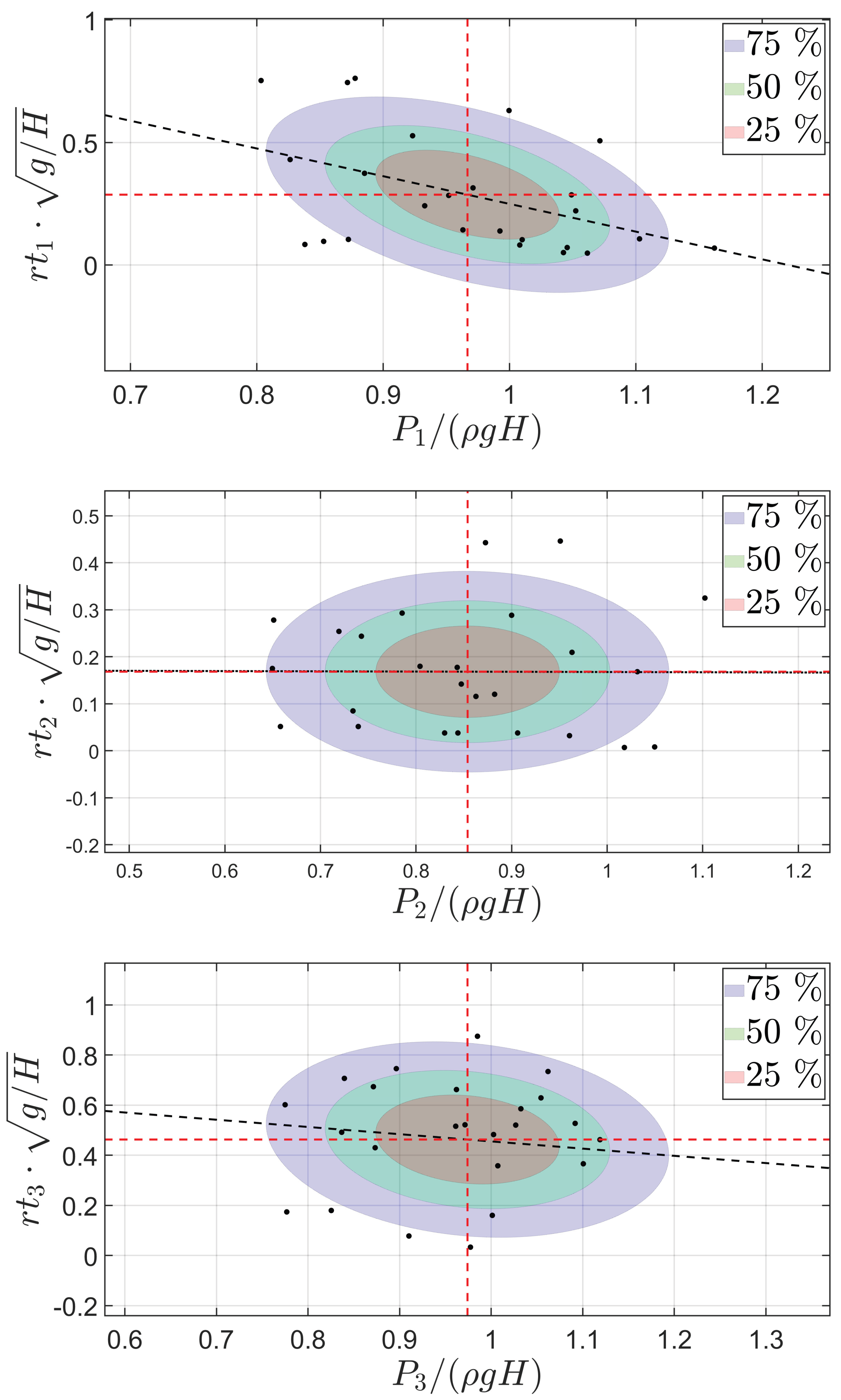
Figure 33.
Median of the pressure time histories for sensor 1 (left), 2 (centre) and 3 (right). Comparison between the data published in [1] with no obstacle, asymmetric and symmetric configurations.
Figure 33.
Median of the pressure time histories for sensor 1 (left), 2 (centre) and 3 (right). Comparison between the data published in [1] with no obstacle, asymmetric and symmetric configurations.
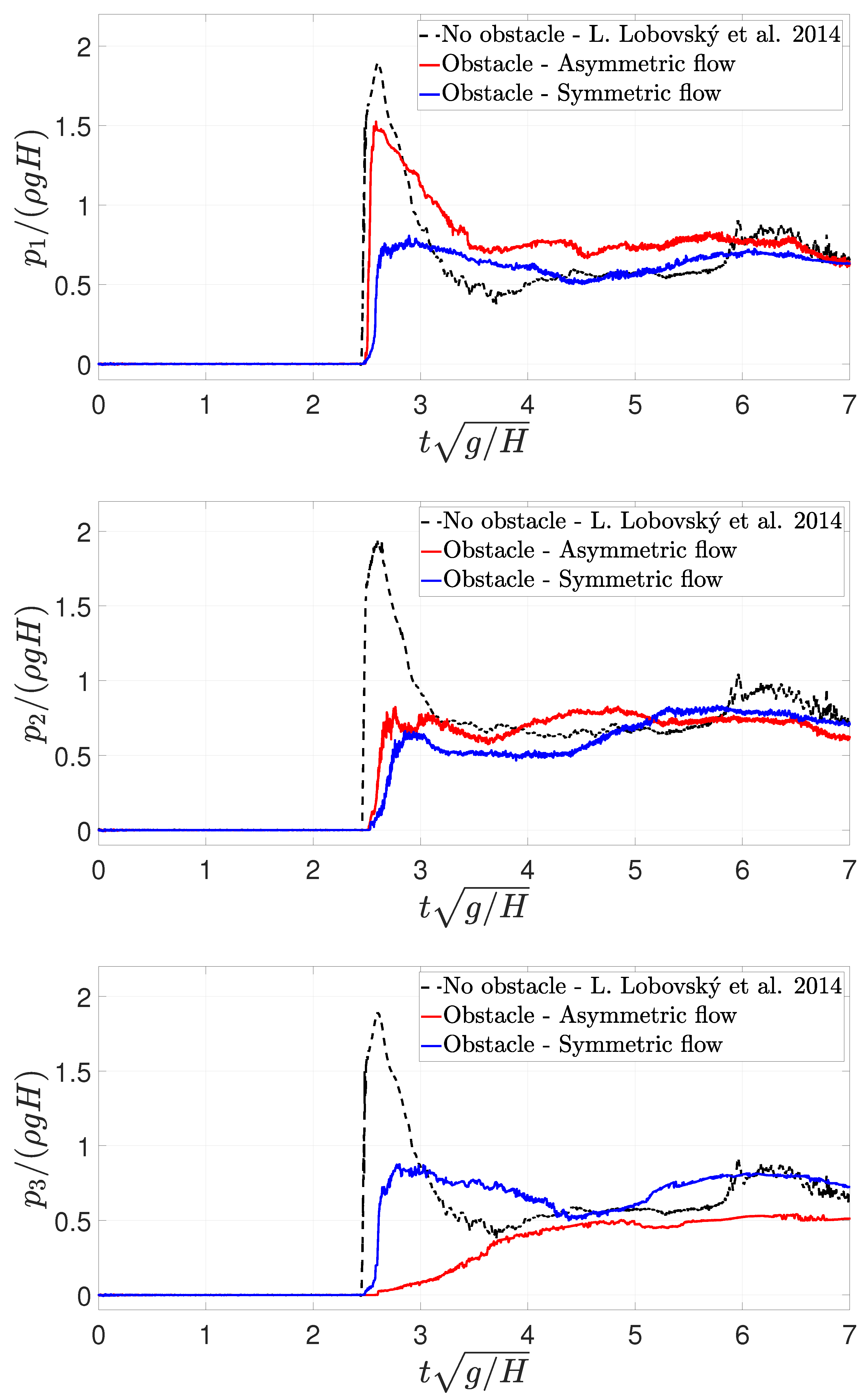
Figure 34.
Median of the maximum pressure peak for sensors 1, 2 and 3. Comparison between the data published in [1] with no obstacle, asymmetric and symmetric configurations.The bars indicate the maximum and minimum recorded pressure peak values.
Figure 34.
Median of the maximum pressure peak for sensors 1, 2 and 3. Comparison between the data published in [1] with no obstacle, asymmetric and symmetric configurations.The bars indicate the maximum and minimum recorded pressure peak values.
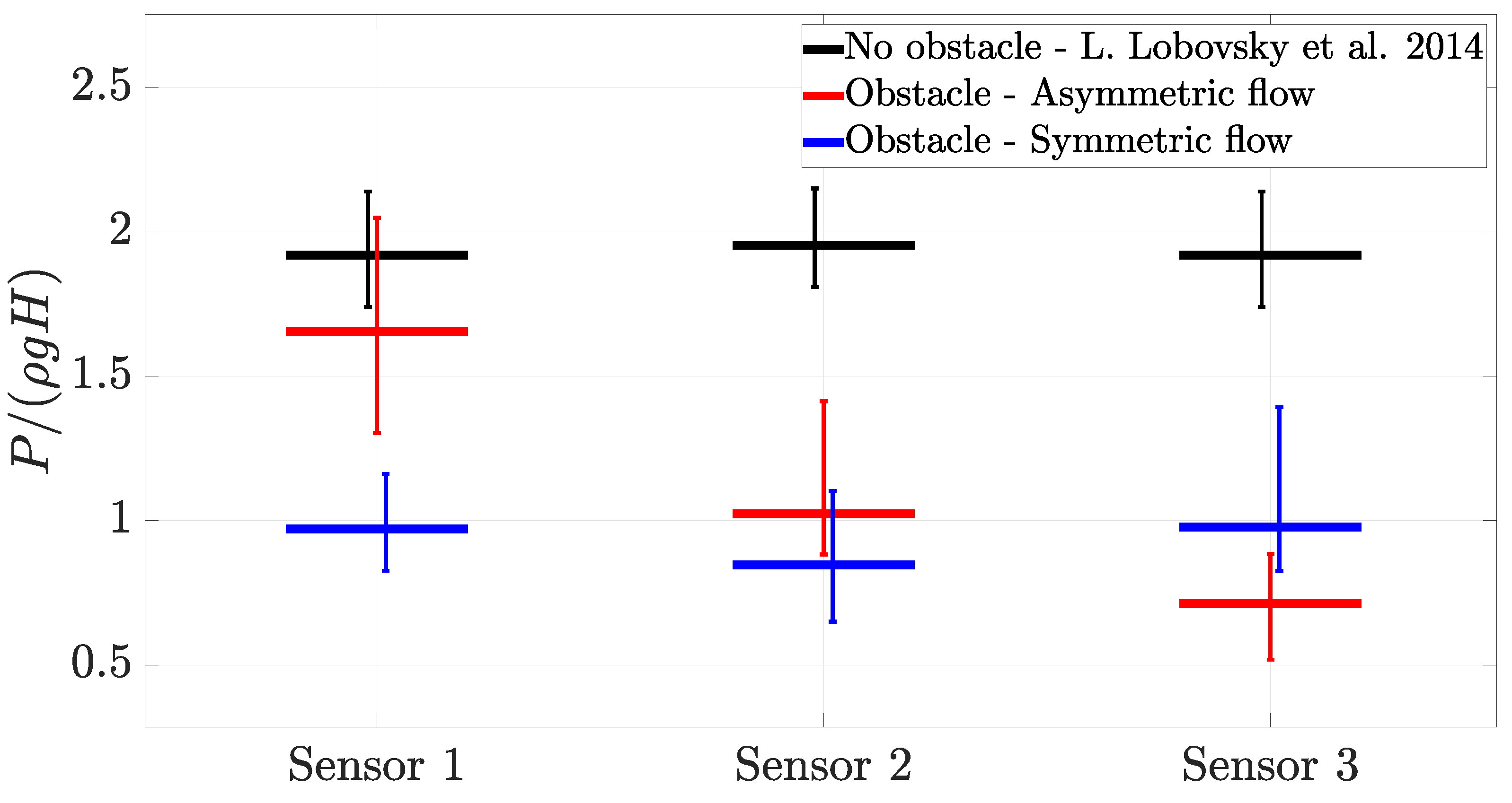

Table 1.
Mechanical properties of the tested water at 25 °C: density, dynamic viscosity and surface tension.
Table 1.
Mechanical properties of the tested water at 25 °C: density, dynamic viscosity and surface tension.
| Temperature [K] | Density [kg/m3] | Dynamic viscosity [Pa s] | Surface tension [mN/m] |
| 298 | 997 | 72 |
Disclaimer/Publisher’s Note: The statements, opinions and data contained in all publications are solely those of the individual author(s) and contributor(s) and not of MDPI and/or the editor(s). MDPI and/or the editor(s) disclaim responsibility for any injury to people or property resulting from any ideas, methods, instructions or products referred to in the content. |
© 2025 by the authors. Licensee MDPI, Basel, Switzerland. This article is an open access article distributed under the terms and conditions of the Creative Commons Attribution (CC BY) license (http://creativecommons.org/licenses/by/4.0/).
Copyright: This open access article is published under a Creative Commons CC BY 4.0 license, which permit the free download, distribution, and reuse, provided that the author and preprint are cited in any reuse.


