
Submitted:
04 November 2025
Posted:
05 November 2025
You are already at the latest version
Abstract
Electroencephalography (EEG)-based motor imagery (MI) brain–computer interfaces (BCIs) hold significant potential for applications in neuro-rehabilitation and assistive technologies. Yet, their development remains constrained by challenges such as low spatial resolution, vulnerability to noise and artifacts, and pronounced inter-subject variability. Conventional approaches, including common spatial patterns (CSP) and convolutional neural networks (CNNs), often exhibit limited robustness, weak generalization, and reduced interpretability. To overcome these limitations, we introduce EEG-GCIRNet, a Gaussian connectivity-driven EEG imaging representation network coupled with a regularized LeNet architecture for MI classification. Our method integrates raw EEG signals with topographic maps derived from functional connectivity into a unified variational autoencoder framework. The network is trained with a multi-objective loss that jointly optimizes reconstruction fidelity, classification accuracy, and latent space regularization. The model’s interpretability is enhanced through its variational autoencoder design, allowing for qualitative validation of its learned representations. Experimental evaluations demonstrate that EEG-GCIRNet consistently outperforms both baseline models and state-of-the-art MI classification methods. Beyond classification accuracy, analysis of the reconstructed connectivity maps and latent space visualizations confirms that the model captures physiologically relevant patterns and learns a well-disentangled feature space. These findings suggest that EEG-GCIRNet provides a robust and interpretable end-to-end framework for EEG-based BCIs, advancing the development of reliable neurotechnology for rehabilitation and assistive applications.
Keywords:
deep learning
; EEG
; motor imagery
; gaussian connectivity
; imaging
; explainability
1. Introduction
Engineering has emerged as a cornerstone in addressing pressing global health challenges, as emphasized in UNESCO’s Engineering for Sustainable Development report (2021), which recognizes the discipline as a central pillar of the 2030 Agenda. Among the Sustainable Development Goals, SDG 3 — “ensure healthy lives and promote well-being for all at all ages” — underscores the need for accessible and affordable technologies to strengthen medical diagnostics and healthcare delivery [1]. Within this framework, brain–computer interfaces (BCIs) have gained increasing international attention for their potential to revolutionize human–machine interaction in clinical, rehabilitative, and assistive domains. Beyond their scientific and societal impact, BCIs are also economically significant: the global market is projected to reach USD 2.21 billion by 2025 and expand further to USD 3.60 billion by 2030, with a compound annual growth rate (CAGR) of 10.29 [2]. This convergence of societal need, technological innovation, and market growth highlights BCIs as a key enabler for sustainable health solutions.
Within this landscape, electroencephalography (EEG) has become a foundational technology for BCI implementation, owing to its non-invasive nature, low cost, portability, and high temporal resolution [3]. EEG captures the brain’s electrical activity through scalp-mounted electrodes and enables the use of advanced signal processing techniques such as event-related potentials (ERPs), which are widely used to assess cognitive and motor functions [4]. These features have established EEG as the technological backbone of many modern BCI platforms, allowing for the decoding of neural signals to control external devices without requiring muscular input [5]. Among the various paradigms, motor imagery (MI)—the mental rehearsal of movement without physical execution—has demonstrated remarkable clinical potential in post-stroke rehabilitation, neuroprosthetic control, and assistive technologies such as robotic wheelchairs and virtual spellers [6].
Despite its versatility, EEG-based BCI systems face inherent structural limitations, primarily due to the physical and physiological nature of the recorded brain signals [7]. These constraints compromise both signal quality and interpretability, directly affecting their clinical and functional applicability [8]. One of the most critical challenges is inter-subject variability, which introduces significant inconsistency in neural activation patterns and undermines the generalization of classification models used in BCI [9,10]. This variability has been strongly linked to the phenomenon known as BCI illiteracy, where a substantial subset of users is unable to gain intentional control of the system, even after repeated training sessions [11,12]. Beyond its technical implications, this limitation poses a fundamental challenge to the inclusion and scalability of BCI technologies in real-world clinical settings, where system adaptability to diverse neurophysiological profiles is essential [13]. Another key obstacle in the development of EEG-based BCI systems is their limited spatial resolution, which is inherently constrained by volume conduction effects. Unlike imaging modalities such as functional magnetic resonance imaging (fMRI) or Magnetoencephalography (MEG), EEG suffers from spatial distortions because neural electrical signals must traverse multiple layers with varying conductivities—such as the skull and scalp—before being recorded at the surface electrodes [14]. This biophysical phenomenon results in signal mixing across electrodes, making it difficult to accurately localize cortical activity [14]. Consequently, spatial specificity is reduced in applications that require fine-grained identification of motor or sensory regions, ultimately limiting the system’s performance in rehabilitation, neurofeedback, and precision control tasks [15].
In this context, various classical signal processing and machine learning methods have been proposed to improve signal quality and extract discriminative features from EEG recordings, particularly in MI paradigms. Among the earliest approaches, time–frequency domain techniques such as the short-time Fourier transform (STFT) [16] and the wavelet transform [17,18] have proven effective in decomposing EEG signals into more informative components by capturing their non-stationary nature. These tools facilitate the identification of relevant brain rhythms, particularly the (8–12 Hz) and (13–30 Hz) bands, which have been widely linked to movement execution and motor imagery [19]. Additionally, the filter bank common spatial patterns (FBCSP) approach extends this principle by dividing the EEG into multiple frequency sub-bands and applying the CSP algorithm to each of them, thereby enhancing class discrimination [20]. While these strategies improve the signal-to-noise ratio (SNR), their effectiveness depends on fixed or heuristically defined frequency ranges, which limits their adaptability to inter-subject spectral variability [21]. Furthermore, CSP variants—such as regularized CSP, discriminative CSP, and sparse CSP—attempt to mitigate overfitting and improve generalization, but remain noise-sensitive and often require subject-specific calibration [22]. Crucially, these approaches provide limited robustness to the spatial distortions inherent in EEG, caused by volume conduction, which restricts their ability to resolve cortical sources with precision and thus limits their performance in tasks requiring spatial specificity [23].
Conversely, recent approaches have leveraged deep learning, particularly convolutional neural networks (CNNs), to extract hierarchical representations from raw EEG signals. Architectures such as EEG network (EEGNet) [24], shallow convolutional network (ShallowNet) and deep convolutional network (DeepConvNet) [25], and temporal–channel fusion network (TCFusionNet) [26] have shown potential in MI classification by learning spatial and temporal patterns without the need for manual feature engineering. These models exhibit increased robustness to noise and, in some cases, can implicitly compensate for spatial distortions through convolutional kernels. Building on this foundation, kernel-based regularized EEGNet (KREEGNet) [27] introduces explicit spatial encodings and specialized convolutional kernels to enhance cortical sensitivity, offering a more targeted solution to the spatial resolution limitations of EEG. Nevertheless, the performance of these architectures remains highly dependent on large, high-quality datasets, and deeper networks are particularly prone to overfitting. Moreover, achieving robust model generalization remains a significant challenge, particularly due to high inter-subject variability in EEG patterns. As a result, most approaches still rely on subject-specific calibration or employ transfer learning strategies to adapt models across individuals [28]. Beyond CNNs, cutting-edge research has begun to explore attention mechanisms, transformer architectures, and generative modeling [29]. Transformer-based models have shown strong performance in capturing long-range temporal dependencies and improving generalization across subjects. For instance, convolutional Transformer network (CTNet) [30] leverages multi-head self-attention to dynamically extract discriminative spatial-temporal features. Similarly, spatial–temporal transformer models have demonstrated robustness in multi-scale temporal feature extraction [31]. Complementary generative approaches, including autoencoders and variational autoencoders (VAEs), have been employed for nonlinear denoising and unsupervised feature learning [32,33]; however, these models inadvertently discard class-discriminative information unless properly regularized [33]. More recently, multimodal and diffusion-based transformer models have been proposed to integrate spatial, temporal, and topological EEG dynamics [34], though their architectural complexity and computational demands may limit their application in real-time or clinical settings [32].
In addition to approaches based on local or spatial features, EEG representation through connectivity models has been extensively explored, including spectral, structural, directed, and functional connectivity. Spectral connectivity, based on measures such as coherence and spectral entropy, allows for the capture of phase and power relationships between cortical regions, but may be sensitive to noise and the choice of frequency bands [35]. Structural connectivity, typically derived from neuroimaging techniques such as MRI, is difficult to obtain from EEG and is rarely integrated directly into non-invasive applications [36]. Directed connectivity aims to identify causal relationships between regions using metrics like partial directed coherence or dynamic causal modeling [37]; although it enhances interpretability, it often entails significant computational complexity. Functional connectivity, by contrast, has been the most widely applied in EEG contexts due to its ability to model statistical dependencies. As a recent advancement, Gaussian functional connectivity has been proposed as a more robust representation for capturing nonlinear spectral-domain relationships. This formulation was employed in the kernel cross-spectral functional connectivity network (KCS-FCNet) model [38], which integrates kernelized functional connectivity to enhance class discrimination in motor imagery paradigms. Overall, although various forms of connectivity have been explored in conjunction with deep learning, their direct application has yet to mature to a point that effectively addresses critical challenges such as inter-subject variability and limited spatial resolution [36].
Here, we introduce EEG-GCIRNet—a Gaussian connectivity–driven EEG imaging representation Network. This framework is designed to transform functional connectivity patterns into a robust image-based representation for MI classification using a variational autoencoder. Unlike conventional approaches, our method creates a rich representation by generating topographic maps from Gaussian functional connectivity, which model nonlinear spatial–functional dependencies across brain regions. Our EEG-GCIRNet framework comprises three key stages:
- –
- Image-based encoding: Gaussian connectivity-based image representations are encoded into a shared latent space that captures complementary spatio-temporal and frequency information, enabling more discriminative and interpretable feature representations.
- –
- Multi-objective training: The model is optimized through a composite loss that jointly enforces reconstruction fidelity, classification accuracy, and latent space regularization, enhancing robustness to noise and mitigating inter-subject variability.
- –
- VAE-based interpretability: The framework’s variational autoencoder design enables direct qualitative assessment. By analyzing the reconstructed topographic maps and visualizing the latent space, we can validate the physiological relevance of the learned features and confirm the model’s ability to create a well-separated feature space, enhancing overall transparency.
Experimental evaluations on benchmark MI datasets demonstrate that EEG-GCIRNet consistently outperforms state-of-the-art baselines, achieving superior classification accuracy. Moreover, interpretability analyses reveal distinct functional connectivity structures that align with known motor cortical regions, offering neurophysiological validation of the model’s learned representations. As such, the proposed framework advances the development of robust and interpretable EEG-based BCIs, paving the way for adaptive neurotechnologies in rehabilitation, assistive communication, and motor recovery. By combining multimodal encoding, multi-objective learning, and explainable AI, EEG-GCIRNet contributes a reproducible and scalable paradigm for addressing two of the most persistent challenges in EEG-based BCI research: inter-subject variability and limited spatial specificity.
2. Materials and Methods
2.1. GIGAScience Dataset for EEG-based Motor Imagery
The Giga Motor Imagery–DBIII (GigaScience) dataset, publicly available at http://gigadb.org/dataset/100295 (accessed on 1 July 2025), provides one of the most comprehensive EEG corpora for MI analysis. The dataset comprises recordings from 52 healthy participants (50 with usable data), each performing a single EEG-MI session. Every session consists of five to six experimental blocks, with each block containing approximately 100–120 trials per class. Each trial spans seven seconds and follows a fixed timeline: an initial blank screen (0–2 s), a visual cue indicating either left- or right-hand MI (2–5 s), and a concluding blank interval (5–7 s). Inter-trial intervals vary randomly between 0.1 s and 0.8 s to mitigate anticipatory bias, as illustrated in Figure 1. EEG signals were recorded at a sampling frequency of 512 Hz using a 64-channel cap arranged according to the international 10–10 electrode placement system. In addition to the MI sessions, the dataset includes recordings of real motor execution and six auxiliary non-task-related events—eye blinks, vertical and horizontal eye movements, head motions, jaw clenching, and resting state—enabling a broader exploration of EEG noise sources and artifact correction. This multimodal composition makes the GigaScience particularly valuable for benchmarking advanced deep learning and connectivity-based EEG decoding frameworks, as it supports both intra-subject and inter-subject generalization studies. [subfigure]justification=centering
Each MI trial is structured for the proposed framework. Let denote a multichannel EEG and its associated MI target label, where represents the EEG recording with C spatial channels and temporal samples, and is a one-hot encoded vector indicating the MI class among Q possible categories.
2.2. Laplacian Filtering and Time Segmentation
To enhance the spatial resolution and mitigate the volume conduction effects inherent in EEG recordings, a Surface Laplacian filter is applied to each trial . This filter acts as a spatial high-pass filter by estimating the second spatial derivative of the scalp potential at each electrode with respect to its neighbors , where . Following the methodology in [39], this is achieved by using spherical splines to project the electrode positions onto a unit sphere, which allows for the interpolation of scalp potentials via Legendre polynomials. The interaction between any pair of electrodes is modeled as:
where is the Legendre Polynomial of order n, is the highest polynomial order considered, is a smoothness constant, and are the 3D electrode positions normalized to a unit-radius sphere. The cosine distance is defined as .
The Laplacian-filtered EEG data, denoted as , is subsequently computed using the weighting matrices derived from the spline interpolation:
where is a column vector of ones, is the identity matrix, and is a regularization parameter. The matrix is a regularized (smoothed) version of . The weighting matrices hold the elements derived from Equation (1), with their specific values determined by the parameter as follows:
where and are the elements of matrices and , respectively. This filtering step produces a spatially enhanced representation that serves as input for the subsequent feature extraction stages.
Further, to focus the analysis exclusively on the period of active motor imagery, the Laplacian-filtered signal is temporally segmented. The time window corresponding to the MI task, specifically between and seconds of each trial, is retained. Let and be the start and end times of the MI segment, and be the sampling frequency, the segmented signal is obtained as:
where the slicing notation indicates the selection of temporal samples from the start index to the end index. For brevity, this segmented signal will be denoted as in the subsequent sections.
2.3. Kernel-Based Cross-Spectral Gaussian Connectivity for EEG Imaging
To model the mutual dependency between EEG channels, we consider any two channels from a given trial (where ). Their mutual dependency can be captured using a stationary kernel , which maps both signals into a reproducing kernel Hilbert space (RKHS) via a nonlinear feature map [40]. Indeed, according to Bochner’s theorem, a sufficient condition for the kernel to be stationary is that it admits a spectral representation [41]:
where is a frequency vector, and is the cross-spectral density between and , derived from the spectral distribution .
Building on this spectral representation, the cross-spectral power within a specific frequency band can be computed via the Fourier transform of the kernel:
where denotes the Fourier transform. This spectral formulation allows capturing both linear and nonlinear dependencies in the frequency domain, making it particularly useful for analyzing brain signals.
A widely used choice for is the Gaussian kernel, which ensures smoothness, locality, and analytic tractability [42]:
where is a bandwidth hyper-parameter.
Inspired by the kernel-based spectral approaches introduced in [38,43], we compute a Gaussian kernel cross-spectral connectivity estimator to encode spatio–frequency interactions among pairwise EEG channels. Specifically, for each EEG channel c, a band-limited spectral reconstruction is obtained as:
where denotes a given frequency bandwidth (rhythm). Then, the Gaussian Function Connectivity (GFC) matrix is derived to quantify the degree of similarity between the spectral representations of all channel pairs, as:
where is a Gaussian kernel with scale parameter . To ensure adaptive sensitivity across rhythms, is estimated as the median of all pairwise Euclidean distances between spectral reconstructions and , . This formulation provides a data-driven normalization of connectivity strength, enabling robust comparison across heterogeneous EEG rhythms and subjects.
Afterward, we propose to compute an EEG connectivity flow from , preserving a direct one-to-one correspondence with the electrode spatial configuration. Specifically, the GFC flow vector holds elements:
where each element represents the mean functional coupling of channel c with all other channels within the given frequency band . The latter compresses the pairwise connectivity information into a compact, channel-wise flow representation while retaining the spatial and spectral data patterns.
To ensure a consistent feature scale for the imaging stage, the GFC flow vectors are normalized across the entire training dataset. Specifically, a channel-wise Min-Max normalization is applied, scaling the connectivity values of each channel to a uniform range of . This procedure preserves the relative topography of neural connectivity while standardizing the input scale, yielding the normalized flow vector for each trial.
2.4. Topographic Map Generation
The final feature engineering step transforms the one-dimensional GFC flow vectors into two-dimensional topographic images, creating a data representation suitable for convolutional neural network (CNN) architectures. For each trial, this process converts the normalized flow vector from each frequency band into a corresponding topographic image .
This transformation is accomplished via spatial interpolation guided by Delaunay triangulation. First, the set of 2D scalp coordinates of the electrodes, , is triangulated. This partitions the electrode layout into a mesh of non-overlapping triangles, where the circumcircle of each triangle contains no other electrode points. This triangulation provides a structured grid for interpolating the connectivity values, where each element is associated with its corresponding coordinate .
To generate the final image, the value for each pixel is computed using barycentric interpolation within its enclosing triangle :
where is the connectivity value at vertex , and are the barycentric coordinates of satisfying and . This procedure is applied across all pixels to render the smooth topographic map . The resulting set of four maps (one for each frequency band) is then stacked to form a multi-channel image, which serves as the final input to the deep learning model.
2.5. EEG-GCIRNet: Multimodal Architecture
The proposed model is a variational autoencoder (VAE) designed to process topographic maps derived from functional connectivity representations. Its architecture relies on a single input stream that learns to extract and encode the most relevant spatial features from the maps, which are then projected into a shared latent space where a multivariate Gaussian distribution is modeled. From this latent space, the model simultaneously performs reconstruction of the topographic maps and classification of motor imagery tasks. These objectives are integrated within a composite loss function that balances reconstruction fidelity, classification accuracy, and latent space regularization. This approach enables the learning of robust and interpretable latent representations capable of capturing discriminative spatial relationships and adapting to the variability and noise inherent in EEG signals.
The core of our framework is a VAE based on the LeNet-5 architecture, which is partitioned into three functional blocks: an encoder, a decoder, and a classifier, all operating on the shared latent space. Let be the multi-channel input image for a given trial, formed by stacking the B topographic maps (one for each frequency band).
The encoder, defined as a function parameterized by , maps the input image Y to the parameters of the posterior distribution . This transformation is realized through a composition of functions, where each function represents a layer in the network:
Here, and are convolutional layers with ReLU activation, and are average pooling layers, and is a fully connected layer with ReLU activation after flattening the feature maps. The resulting hidden representation is then linearly transformed to produce the mean vector and the log-variance vector of the latent space:
The decoder, defined as a function parameterized by , reconstructs the original input image from a latent vector . Its architecture mirrors the encoder by composing functions that progressively up-sample the representation to the original image dimensions:
Here, is a fully connected layer followed by a reshape operation, is a transposed convolutional layer with ReLU activation, and is a final transposed convolutional layer with a Sigmoid activation to ensure the output pixel values are in a normalized range.
Concurrently, the classifier, a function parameterized by , predicts the MI task label probabilities from the same latent vector z. It is implemented as a multi-layer perceptron:
Formally, the latent vector for a given input sample i is computed using the reparameterization trick:
where and denote the mean and variance of the approximate posterior distribution learned by the encoder for sample i, and is drawn from a standard normal distribution. The exponential term ensures the sampled standard deviation remains strictly positive.
The total objective function, , is defined as a weighted sum of the three loss terms:
where
where , , and are hyperparameters controlling the contribution of each term. The first component, , is the normalized mean squared error (NMSE), which evaluates reconstruction accuracy by comparing the original topographic maps () and their reconstructions (), normalized by the dataset’s variance ( is the mean image). The Frobenius norm, , is used for the image-wise error. The second term, , represents the normalized binary cross-entropy (NBCE). It penalizes misclassifications between the true one-hot labels () and predicted probabilities (), while adjusting the loss based on the entropy over an ideal, non-informative prediction (e.g., a uniform distribution ). This maintains a balanced contribution from all classes. Finally, the third term, , is the normalized Kullback–Leibler (KL) divergence between the approximate posterior and a unit Gaussian prior . This regularizes the latent space, promoting smoothness and disentanglement in the learned representations.
This KL divergence term encourages the latent representations to follow a standard normal distribution, promoting structure and generalization. The use of in the denominator prevents this term from dominating the loss in large batches. Taken together, these components ensure that the model jointly optimizes for faithful reconstruction, discriminative performance, and a well-regularized latent structure—crucial for interpretable and generalizable multimodal brain–computer interfaces.
The model is trained by solving the following optimization problem:
where denotes the complete set of trainable parameters in the encoder, decoder, and classifier, respectively.
3. Experimental Set-Up
This work presents EEG-GCIRNet, a framework for MI classification built upon topographic maps derived from functional connectivity. The proposed methodology, illustrated in Figure 2, comprises three primary stages: (i) preprocessing raw EEG signals to compute GFC-based flow vectors; (ii) generating 2D topographic maps from these vectors; and (iii) processing the resulting images with a deep learning architecture for simultaneous classification and reconstruction.
3.1. Stage 1: Signal Preprocessing and Feature Engineering
First, an average reference was applied, which included the original reference electrode to ensure the data retained full rank. Subsequently, a fifth-order Butterworth bandpass filter was applied in the Hz range. To reduce computational load and maintain consistency across the evaluated deep learning models, the filtered signals were resampled from 512Hz to 128Hz [38,44]. This entire pipeline was applied to a subset of 50 subjects from the original dataset; participants 29 and 34 were excluded due to data availability constraints.
Building upon this preprocessed data, the feature engineering process involves applying a Surface Laplacian filter to enhance the spatial resolution of the signals. The data is then temporally segmented to isolate the active MI period, retaining the window from to seconds. This segmented data is further decomposed via band-pass filtering into four functionally distinct frequency bands: (Hz), low-beta (, Hz), mid-beta (, Hz), and high-beta (, Hz). For each frequency band, GFC is computed to quantify the functional relationships between all channel pairs. The resulting connectivity information is then condensed into a normalized, channel-wise flow vector for each band.
3.2. Stage 2: Topographic Map Generation
The second stage of the pipeline transforms the one-dimensional, GFC-based flow vectors into a two-dimensional, image-based representation suitable for processing with a CNN. This conversion is critical as it re-introduces the spatial topography of the EEG electrodes, allowing the model to learn spatially coherent features.
This transformation was achieved via spatial interpolation, a process implemented using the visualization utilities within the MNE-Python library1. For each frequency band, the corresponding flow vector’s values are mapped to the coordinates of the EEG electrodes. A mesh is then constructed over these coordinates using Delaunay triangulation. The pixel values for the final topographic map are subsequently estimated using linear barycentric interpolation within this mesh.This procedure is repeated for each of the four frequency bands (, , , and ), yielding a set of four distinct topographic maps per trial. These maps are then stacked along the channel dimension to form a single, multi-channel image of size . This resulting data structure serves as the final input to the EEG-GCIRNet architecture, providing a rich, spatio-spectral representation of the brain’s functional connectivity during motor imagery.
3.3. Stage 3: EEG-GCIRNet Architecture and Training
The core of this model is a VAE with a convolutional architecture inspired by LeNet-5. This architecture is composed of three interconnected functional blocks operating on a shared latent space: an encoder, a decoder, and a classifier.
The encoder block consists of two sequential pairs of convolutional and average pooling layers, which extract hierarchical spatial features from the input image. These features are then flattened and passed through a dense layer to produce a compact representation, which in turn parameterizes the mean () and log-variance () vectors of the latent space. The decoder mirrors this structure using transposed convolutional layers to upsample the latent representation back to the original image dimensions. Concurrently, the classifier, a simple multi-layer perceptron, operates on the same latent vector to perform the final classification. The detailed layer-wise configuration of the EEG-GCIRNet is summarized in Table 1.
The EEG-GCIRNet model was trained end-to-end by optimizing the composite loss function described in subSection 2.5. The training was performed using the Adam optimizer with an initial learning rate of . The hyperparameters that weight the loss components were set using KerasTuner framework to ensure a balanced contribution from reconstruction, classification, and regularization objectives during training. The model was trained for a total of 200 epochs with a batch size of 64. An early stopping mechanism was employed with a patience of 10 epochs, monitoring the validation loss to prevent overfitting and save the model with the best generalization performance. The dataset was split using a subject-wise cross-validation scheme to ensure that the training and testing sets were independent at the subject level.
3.4. Evaluation Criteria
The performance of the proposed EEG-GCIRNet was rigorously evaluated using a multi-faceted approach. The primary quantitative metric was subject-specific classification accuracy, which was benchmarked against seven baseline and state-of-the-art models. To validate the findings, a robust statistical framework was employed, using a Friedman test to assess overall significance, followed by post-hoc pairwise t-tests for direct model comparisons. The framework’s robustness and generalization capabilities were further analyzed by stratifying subjects into “Good” (with EEGNet accuracy above 80%), “Mid” (with EEGNet accuracy between 60% and 80%), and “Bad” (with EEGNet accuracy below 60%) performance groups, allowing for a targeted assessment of its effectiveness across varying EEG signal qualities.
Beyond quantitative metrics, the evaluation delved into the model’s interpretability by leveraging its variational autoencoder architecture. This qualitative assessment involved two key methods: first, a visual analysis of the reconstructed topographic maps to confirm that the model learned physiologically relevant spatio-spectral patterns; and second, the visualization of the latent space using t-SNE projections to directly inspect the quality of class separability and feature disentanglement. This combined quantitative and qualitative evaluation provides a holistic validation of the EEG-GCIRNet framework, covering its accuracy, statistical significance, and the meaningfulness of its learned internal representations.
4. Results
4.1. MI Classification Performance
Figure 3 illustrates the subject-wise classification performance, where a clear advantage of EEG-GCIRNet becomes evident, particularly in challenging cases. Within the “Bad” group—comprising subjects with low-quality or highly variable EEG signals—conventional models like CSP, ShallowConvNet, and DeepConvNet consistently yield low and unstable results, reflecting their limited ability to handle noise and inter-subject variability. While architectures such as EEGNet and KREEGNet show more stable behavior, their performance remains inconsistent. In stark contrast, EEG-GCIRNet entirely eliminates the ’Bad’ performance group, demonstrating a generalized improvement and a notable reduction in inter-subject variability. This outcome strongly suggests that the model’s variational formulation and latent space regularization provide robust feature encoding, effectively preventing the critical performance failures seen in other architectures [45,46].
EEG-GCIRNet extends its advantage into the “Mid” group, consistently outperforming competing models like TCFusionNet and KREEGNet across most subjects. This stability under intermediate conditions underscores the model’s strong generalization capability, as it delivers reliable performance even with moderately variable EEG signals. These results validate the effectiveness of the variational approach in preserving discriminative information while maintaining training stability [47].
In the “Good” group, where most architectures achieve high accuracy, EEG-GCIRNet performs competitively, matching or exceeding the results of TCFusionNet, KREEGNet, and EEGNet. Critically, its performance is marked by greater consistency across subjects, highlighting its ability to maintain high accuracy without overfitting. This behavior contrasts sharply with deeper architectures like DeepConvNet, which are more susceptible to performance degradation in subject-specific tasks [15].
Collectively, the subject-wise results in Figure 3 underscore that EEG-GCIRNet achieves a superior balance of accuracy, stability, and generalization. This positions it as a highly effective and well-rounded model for EEG decoding [48,49]. The aggregate performance metrics summarized in Table 2 confirm these subject-wise trends. EEG-GCIRNet stands out as the best-performing model overall, achieving the highest average accuracy () and the lowest standard deviation (), which confirms its strong generalization and inter-subject stability.
Notably, while KREEGNet achieves a competitive average accuracy (), its greater performance variability () indicates reduced stability. Taken together, these results position EEG-GCIRNet as the most reliable alternative, outperforming all reference architectures in both classification accuracy and consistency.
To validate that the observed performance differences among the models were statistically meaningful, a rigorous statistical analysis was conducted. A Friedman test was first applied to the subject-wise accuracies of all eight models, yielding a test statistic with a p-value of . This result, being below the software’s detection threshold, allows for the rejection of the null hypothesis of equal medians with a high level of confidence, confirming that significant differences exist across the evaluated architectures.
The nature of these differences is detailed in Figure 4 and Table 3. The subject-wise ranking heatmap (Figure 4) visually confirms the performance tiers, highlighting the consistent top rankings of EEG-GCIRNet and KREEGNet, the intermediate performance of models like TCFusionNet and ShallowConvNet, and the instability of DeepConvNet and CSP. The matrix of p-values from post-hoc pairwise t-tests (Figure 4) further reinforces this, revealing statistically significant differences between the high- and low-performing models.
The summary of these statistical measures in Table 3 provides a conclusive overview. EEG-GCIRNet emerges as the clear top-performing model, securing the lowest average ranking () and the only average p-value indicating strong statistical significance (). This result demonstrates a robust and consistent performance advantage over the other architectures. These findings align perfectly with the accuracy results from Table 2, cementing its reliability as a unimodal image-based model for MI classification.
While the KREEGNet model is its closest competitor with an average ranking of , its higher average p-value () and greater performance variability indicate lower statistical significance and stability compared to EEG-GCIRNet. This consistent advantage is likely attributable to EEG-GCIRNet’s variational formulation, which promotes more uniform representations across subjects. In summary, the statistical analysis positions EEG-GCIRNet as the most prominent model in terms of both accuracy and statistical significance.
4.2. Robustness and Generalization Across Subject Groups
A key advantage of EEG-GCIRNet lies in its ability to generalize across subjects and its robustness to the high inter-subject variability inherent in EEG data. To assess this, a stratified analysis was performed based on signal quality, with the performance distributions for each model shown in Figure 5.
In high-quality signal conditions (“Good” group, Figure 5), all methods perform well ( accuracy). However, EEG-GCIRNet is distinguished by its more compact distribution concentrated at the upper end of the accuracy range, indicating superior inter-subject stability and performance consistency. This behavior, likely stemming from its latent space regularization, contrasts with the wider distributions of models like DeepConvNet and CSP, which reflect greater variability. This advantage becomes more pronounced in the “Mid” group (Figure 5), which represents subjects with moderate signal quality. While most architectures exhibit broader and less stable performance distributions, EEG-GCIRNet maintains a distribution centered around high accuracy values () with only moderate dispersion. This demonstrates its ability to preserve generalization and deliver stable performance even as class separability decreases.
The most compelling evidence of the model’s robustness is found in the “Bad” group (Figure 5), which reflects the most challenging EEG conditions. Here, most models exhibit broad distributions shifted toward low accuracies (). Crucially, EEG-GCIRNet is the only model for which this group is empty, reaffirming its resilience against signal degradation and its superior stability, as previously suggested by the global accuracy and ranking analyses.
These distributional advantages translate directly into substantial accuracy gains, as summarized in Table 4. The improvements are most pronounced for subjects who perform poorly with baseline models. In the “Bad” group, where EEGNet achieves an average accuracy of only , EEG-GCIRNet provides a remarkable increase, elevating the average performance to . A substantial gain of is also observed in the “Mid” group. Conversely, for the “Good” group, where the baseline performance is already high, EEG-GCIRNet maintains a comparable accuracy with only a slight decrease (). This confirms that the significant gains for challenging cases are not achieved at the expense of performance in high-quality signal conditions.
The subject-wise nature of this improvement is illustrated in Figure 6, which highlights the performance leap achieved by EEG-GCIRNet compared to the EEGNet baseline. While most participants benefit from moderate accuracy gains, a notable subset—including subjects 21, 40, 24, 30, 42, 9, 15, and 7 exhibit a pronounced transition from “Bad” to “Good” performance levels. For several of these individuals (e.g., subjects 24, 9, and 7), accuracy exceeds the threshold. This performance leap reinforces the hypothesis that latent space modeling in EEG-GCIRNet not only mitigates the limitations of signal noise but also provides an effective mechanism for uncovering discriminative structure in signals previously deemed uninformative.
These findings are highly relevant for developing inclusive BCI systems. The fact that several initially low-performing individuals achieve high accuracy suggests that EEG-GCIRNet can serve a corrective function within BCI pipelines, enhancing usability and consistency. This benefit extends to “Mid-performing” users as well, many of whom are elevated to the high-performing category. This corrective and enhancing capability supports the use of latent generative models in real-world BCI contexts, where adaptability and generalization are critical [54,55,56].
4.3. Interpretability and Internal Model Dynamics
To understand the mechanisms behind EEG-GCIRNet’s robust performance, we analyzed its internal dynamics and learned representations. The results reveal that the model is not a “black box” but a well-designed framework that adapts its learning strategy, captures physiologically meaningful patterns, and creates a highly effective feature space.
4.3.1. Adaptive Learning Through Loss Weight Reorganization
A key feature of EEG-GCIRNet is its ability to adapt its optimization priorities based on signal quality. The distributions of the three loss component weights, presented in Figure 7, reveal a distinct internal reorganization between the “Good” and “Mid” performance groups. This behavior highlights the model’s inherent ability to promote a balanced interaction between reconstruction accuracy, discriminative capacity, and latent space stability.
For the “Good” group, the weights for reconstruction (REC), classification (CLA), and latent space regularization (REG) are relatively balanced (modes: , , and , respectively). This indicates a harmonious optimization between reconstruction accuracy, discriminative capacity, and latent space stability. The slight predominance of the REG component suggests a focus on maintaining a coherent latent structure, which aligns with recent findings on the importance of regularization for robust performance [57]. In contrast, for the “Mid” group, the model distinctly reorganizes its priorities. The REG component remains dominant (mode: ), but the CLA weight is significantly reduced (mode: ) in favor of REC (mode: ). This shift indicates that when faced with less discriminative signals, the model prioritizes learning a stable and faithful representation of the input data over immediate classification accuracy. This adaptive strategy, where internal representation optimization substitutes for explicit discriminative signals, is a known characteristic of robust unimodal systems [47].
4.3.2. Qualitative analysis of learned representations
The adaptive weighting strategy directly influences the quality of the learned representations, which can be assessed by analyzing the decoder’s output. Figure 8 and Figure 9 present the class-specific reconstructions for a representative “Good” subject (i.e., 14) and “Mid” subject (i.e., 27).
For subject 14, the reconstructions are spatially homogeneous, reflecting the “Good” group’s emphasis on a stable, regularized latent space. Conversely, for subject 27, the reconstructions are sharper and more structurally defined. This aligns perfectly with the “Mid” group’s increased weighting of the reconstruction (REC) loss, which encourages the model to preserve structural fidelity. The ability to generate coherent and class-consistent topographic maps, even for mid-performing subjects, demonstrates that the VAE is successfully capturing physiologically relevant spatio-spectral patterns from the connectivity data [47,58].
4.3.3. Structure and Separability of the Latent Space
The ultimate outcome of the model’s adaptive learning and representation quality is a well-structured and discriminative latent space. To visualize this, t-SNE projections were applied to the latent representations of subjects 14 and 27 (Figure 10).
For the high-performing subject 14 (Figure 10), the projection reveals two clearly differentiated and cohesive clusters corresponding to the left- and right-hand MI classes. This well-defined separation confirms that the model has learned a highly discriminative latent space, which is consistent with the subject’s high classification accuracy. For the mid-performing subject 27 (Figure 10), the classes are still largely separable, though with some regions of overlap. This is typical for signals with lower quality, where features are partially discriminative but affected by noise [45,46,59].
Taken together, these visualizations confirm that EEG-GCIRNet’s VAE-based design successfully creates a more structured and discriminative latent space than is typically achievable with standard architectures. This underscores the critical role of latent space regularization in adapting to inter-subject variability and improving generalization, even in the presence of noisy inputs [60,61].
5. Discussion
The results obtained with the proposed EEG-GCIRNet architecture provide valuable insights into how model design and latent regularization can jointly address key challenges in motor imagery decoding. This study demonstrated that by transforming functional connectivity into an image-based representation and processing it with a variational autoencoder, it is possible to create a BCI framework that is not only highly accurate but also robust and interpretable. The model achieved remarkable performance across subjects, reaching the highest average accuracy () and the lowest inter-subject variability among all evaluated methods, confirming the efficacy of this unimodal, VAE-based approach.
A key contribution of this work lies in its direct response to the critical challenges of inter-subject variability and “BCI illiteracy”. The most compelling finding was the complete elimination of the “Bad” performance group (Figure 5), coupled with substantial accuracy gains of and pp for the “Bad” and “Mid” groups, respectively (Table 4). This demonstrates the profound robustness of EEG-GCIRNet in handling noisy or low-separability EEG signals, where conventional architectures typically fail. By elevating the performance of these challenging subjects, the framework serves a corrective function, suggesting a promising path toward more inclusive and reliable BCI systems that can adapt to a wider range of users.
The mechanism underlying this robustness appears to be the model’s sophisticated, adaptive learning strategy. The analysis of the loss weight distributions (Figure 7) revealed that EEG-GCIRNet is not a static “black box” but dynamically reorganizes its optimization priorities based on signal quality. For subjects with high-quality signals, it maintains a harmonious balance between reconstruction, classification, and regularization. For subjects with more challenging signals, it strategically prioritizes representation learning (REC loss) over immediate classification (CLA loss). This intelligent trade-off is visually confirmed by the qualitative analysis of the reconstructions (Figure 8 and Figure 9), which shows that the model consistently generates spatially coherent and physiologically plausible connectivity maps. This behavior supports the notion that a well-regularized and accurately reconstructed representation is a prerequisite for effective classification, especially in noisy conditions.
The ultimate outcome of this adaptive process is the creation of a well-structured and discriminative latent space. The t-SNE visualizations (Figure 10) provide direct evidence that the encoder successfully learns to disentangle the features of different MI classes, creating clearly separated clusters for high-performing subjects and maintaining reasonable separation even for mid-performing subjects. This demonstrates that the variational formulation and structured latent regularization are the primary drivers of the model’s superior performance, allowing it to move beyond the limitations of conventional architectures that often struggle with noisy or overlapping feature distributions.
Finally, the statistical analysis (Figure 4, Table 3) confirms the superiority of EEG-GCIRNet, which achieved the lowest average ranking () and the most significant p-value (). This indicates that the observed performance gains are not random fluctuations but a consistent outcome of the model’s design. By learning robust latent structures directly from connectivity-based topographic representations, EEG-GCIRNet emerges as a reliable, interpretable, and computationally efficient framework for motor imagery decoding. It effectively balances accuracy, generalization, and representational stability, allowing it to adapt to diverse subject profiles and maintain strong performance across varying signal quality conditions while preserving a physiologically consistent representational organization.
6. Concluding Remarks
In this work, we introduced EEG-GCIRNet, a unimodal framework based on a variational autoencoder designed to process topographic representations of functional connectivity for motor imagery classification. Through a comprehensive analysis, we demonstrated that this approach effectively addresses the persistent challenges of low accuracy and high inter-subject variability in EEG-based BCIs. The findings confirm that our proposed method not only sets a new benchmark for performance but also provides a robust and interpretable solution.
The primary contribution of this study is the demonstration of superior classification performance. EEG-GCIRNet achieved the highest average accuracy () and, critically, the lowest inter-subject variability () among all evaluated state-of-the-art and baseline models. The statistical analysis confirmed that this performance advantage is significant (), establishing EEG-GCIRNet as a highly reliable and consistent framework for MI decoding.
Perhaps the most significant finding is the model’s robustness in handling challenging EEG signals. By providing substantial accuracy gains for both “Mid” () and “Bad” () performance groups, and by completely eliminating the “Bad” group, EEG-GCIRNet proved its ability to mitigate the effects of BCI illiteracy. This corrective capability suggests that the framework can make BCI technology accessible and effective for a much broader range of users, a crucial step toward the development of inclusive neurotechnology.
This robust performance is driven by the model’s adaptive, multi-objective learning strategy. The analysis of the loss component weights revealed that EEG-GCIRNet dynamically prioritizes its learning objectives, balancing reconstruction, classification, and regularization, based on the quality of the input signals. This intelligent mechanism enables the creation of a well-structured and disentangled latent space, as confirmed by reconstruction and t-SNE analyses. This demonstrates that the model’s success is not a "black box" phenomenon but a direct result of its principled variational design, which effectively learns physiologically meaningful representations even from noisy data.
Despite the promising results, this study has several limitations that must be acknowledged. First, the model was trained and evaluated exclusively on a single motor imagery dataset. This constrains the generalizability of our findings to other BCI paradigms (e.g., P300, SSVEP) or datasets with different characteristics. Second, although the model demonstrated adaptive behavior, the hyperparameters weighting the loss components were static. This fixed weighting may not be optimal for all subjects, and no strategies for dynamic, performance-based adaptation were explored. Finally, our interpretability analysis, while insightful, remains indirect. The analysis of reconstructions and latent space provides a high-level understanding but does not offer the granular, feature-level attribution that techniques like attention-based visualization can provide.
The findings and limitations of this study open several avenues for future research. To address generalizability, the next logical step is to evaluate the EEG-GCIRNet framework on more diverse and larger-scale datasets, including different BCI paradigms and clinical populations. Furthermore, we propose exploring extensions of the model that incorporate dynamic weighting mechanisms for the loss components, which could allow for even greater subject-specific adaptation. We also plan to investigate hybrid architectures, particularly those based on Transformers, to enhance the fusion of raw temporal EEG signals with our connectivity-derived topographic maps, potentially creating a more powerful, end-to-end model. Finally, integrating complementary interpretability techniques, such as feature attribution or attention-based visualization methods, will be crucial for providing a more precise understanding of the model’s decision-making process at the clinical level.
Author Contributions
Conceptualization, A.G.-R., D.F.C.-H, D.C.-P, A.M.A.-M. and G.C.-D.; data curation, A.G.-R., D.F.C.-H; methodology, A.G.-R., D.F.C.-H, D.C.-P, A.M.A.-M.; project administration, D.C.-P, A.M.A.-M. and G.C.-D.; supervision, D.C.-P, A.M.A.-M. and G.C.-D.; resources, D.C.-P, A.M.A.-M. and G.C.-D. All authors have read and agreed to the published version of the manuscript.
Funding
Authors gratefully acknowledge support from the program: “Alianza científica con enfoque comunitario para mitigar brechas de atención y manejo de trastornos mentales relacionados con impulsividad en Colombia (ACEMATE)-91908.” This research was supported by the project: “Sistema multimodal apoyado en juegos serios orientado a la evaluación e intervención neurocognitiva personalizada en trastornos de impulsividad asociados a TDAH como soporte a la intervención presencial y remota en entornos clínicos, educativos y comunitarios-790-2023,” funded by the Colombian Ministry of Science, Technology and Innovation (Minciencias). G. Castellanos-Dominguez also acknowledges support from the project: “Sistema de visión artificial para el monitoreo y seguimiento de efectos analgésicos y anestésicos administrados vía neuroaxial epidural en población obstétrica durante labores de parto para el fortalecimiento de servicios de salud materna del Hospital Universitario de Caldas-SES HUC” (Hermes 57661), funded by Universidad Nacional de Colombia.
Institutional Review Board Statement
Not applicable
Data Availability Statement
The databases used in this study are public and can be found at the following links:http://gigadb.org/dataset/100295 (accessed on 1 July 2025).
Conflicts of Interest
The authors declare no conflicts of interest.
References
- Nair-Bedouelle, S. Engineering for sustainable development: Delivering on the sustainable development goals; United Nations Educational, Scientific, and Cultural Organization, 2021.
- Mordor Intelligence. Brain-Computer Interface Market - Growth, Trends, COVID-19 Impact, and Forecasts (2025 - 2030), 2025.
- Chaudhary, U. , Non-invasive Brain Signal Acquisition Techniques: Exploring EEG, EOG, fNIRS, fMRI, MEG, and fUS; 2025; pp. 25–80. [CrossRef]
- Spanos, M.; Gazea, T.; Triantafyllidis, V.; Mitsopoulos, K.; Vrahatis, A.; Hadjinicolaou, M.; Bamidis, P.D.; Athanasiou, A. Post Hoc Event-Related Potential Analysis of Kinesthetic Motor Imagery-Based Brain-Computer Interface Control of Anthropomorphic Robotic Arms. Electronics 2025, 14. [Google Scholar] [CrossRef]
- Lionakis, E.; Karampidis, K.; Papadourakis, G. Current trends, challenges, and future research directions of hybrid and deep learning techniques for motor imagery brain–computer interface. Multimodal Technologies and Interaction 2023, 7, 95. [Google Scholar] [CrossRef]
- Saibene, A.; Caglioni, M.; Corchs, S.; Gasparini, F. EEG-Based BCIs on Motor Imagery Paradigm Using Wearable Technologies: A Systematic Review. Sensors 2023, 23. [Google Scholar] [CrossRef]
- Singh, A.; Hussain, A.; Lal, S.; Guesgen, H. A comprehensive review on critical issues and possible solutions of motor imagery based electroencephalography brain-computer interface. Sensors 2021, 21, 2173. [Google Scholar] [CrossRef] [PubMed]
- Bouazizi, S.; Ltifi, H. Enhancing accuracy and interpretability in EEG-based medical decision making using an explainable ensemble learning framework application for stroke prediction. Decision Support Systems 2023, 178, 114126. [Google Scholar] [CrossRef]
- Kim, D.; Shin, D.; Kam, T. Bridging the BCI illiteracy gap: a subject-to-subject semantic style transfer for EEG-based motor imagery classification. Frontiers in Human Neuroscience 2023, 17, 1194751. [Google Scholar] [CrossRef] [PubMed]
- Maswanganyi, R.; Tu, C.; Pius, O.; Du, S. Statistical Evaluation of Factors Influencing Inter-Session and Inter-Subject Variability in EEG- Based Brain Computer Interface. IEEE Access 2022, PP, 1–1. [Google Scholar] [CrossRef]
- Saha, S.; Baumert, M. Intra- and inter-subject variability in EEG-based sensorimotor brain-computer interface: A review. Frontiers in Computational Neuroscience 2020, 13, 87. [Google Scholar] [CrossRef]
- Horowitz, A.; Guger, C.; Korostenskaja, M. What External Variables Affect Sensorimotor Rhythm Brain-Computer Interface (SMR-BCI) Performance? HCA Healthcare Journal of Medicine 2021, 2. [Google Scholar] [CrossRef]
- Raza, A.; Yusoff, M.Z. Deep Learning Approaches for EEG-Motor Imagery-Based BCIs: Current Models, Generalization Challenges, and Emerging Trends. IEEE Access 2025, 13, 151866–151893. [Google Scholar] [CrossRef]
- Wang, Y.; Nakanishi, M.; Zhang, D. EEG-based brain–computer interfaces. In Brain–Computer Interface Systems; Springer, 2019; pp. 131–155. [CrossRef]
- Köllőd, C.M.; Adolf, A.; Iván, K.; Márton, G.; Ulbert, I. Deep Comparisons of Neural Networks from the EEGNet Family. Electronics 2023, 12. [Google Scholar] [CrossRef]
- Velasco, I.; Sipols, A.; Simon, C.; Pastor, L.; Bayona, S. Motor imagery EEG signal classification with a multivariate time series approach. BioMedical Engineering OnLine 2023, 22. [Google Scholar] [CrossRef]
- Liu, Z.; Wang, L.; Xu, S.; Lu, K. A multiwavelet-based sparse time-varying autoregressive modeling for motor imagery EEG classification. Computers in Biology and Medicine 2022, 155, 106196. [Google Scholar] [CrossRef] [PubMed]
- Atla, K.G.R.; Sharma, R. Motor imagery classification using a novel CNN in EEG-BCI with common average reference and sliding window techniques. Alexandria Engineering Journal 2025, 120, 532–546. [Google Scholar] [CrossRef]
- Pfurtscheller, G.; Lopes da Silva, F.H. Event-related EEG/MEG synchronization and desynchronization: basic principles. Clinical neurophysiology 1999, 110, 1842–1857. [Google Scholar] [CrossRef] [PubMed]
- Ang, K.K.; Chin, Z.H.; Zhang, H.; Guan, C. Filter bank common spatial pattern algorithm on BCI competition IV datasets 2a and 2b. In Proceedings of the 2008 IEEE International Joint Conference on Neural Networks (IEEE World Congress on Computational Intelligence). IEEE; 2008; pp. 2390–2397. [Google Scholar] [CrossRef]
- Lotte, F.; Bougrain, L.; Cichocki, A.; Clerc, M.; Congedo, M.; Rakotomamonjy, A.; Yger, F. A review of classification algorithms for EEG-based brain–computer interfaces: a 10 year update. Journal of Neural Engineering 2018, 15. [Google Scholar] [CrossRef]
- Akuthota, S.; Kumar, K.; Chander, J. A Complete Survey on Common Spatial Pattern Techniques in Motor Imagery BCI. Journal of Scientific and Innovative Research 2023, 12, 40–49. [Google Scholar] [CrossRef]
- Pan, L.; Wang, K.; Huang, Y.; Sun, X.; Meng, J.; Yi, W.; Xu, M.; Jung, T.P.; Ming, D. Enhancing motor imagery EEG classification with a Riemannian geometry-based spatial filtering (RSF) method. Neural Networks 2025, p. 107511. [CrossRef]
- Deng, X.; Zhang, B.; Yu, N.; Liu, K.; Sun, K. Advanced TSGL-EEGNet for Motor Imagery EEG-Based Brain-Computer Interfaces. IEEE Access 2021, PP, 1–1. [Google Scholar] [CrossRef]
- Roots, K.; Muhammad, Y.; Muhammad, N. Fusion convolutional neural network for cross-subject EEG motor imagery classification. Computers 2020, 9, 72. [Google Scholar] [CrossRef]
- Riyad, M.; Khalil, M.; Abdellah, A. A novel multi-scale convolutional neural network for motor imagery classification. Biomedical Signal Processing and Control 2021, 68, 102747. [Google Scholar] [CrossRef]
- Tobon-Henao, M.; Álvarez Meza, A.; Castellanos-Dominguez, G. Kernel-based Regularized EEGNet using Centered Alignment and Gaussian Connectivity for Motor Imagery Discrimination 2023. [CrossRef]
- Liang, Z.; Zheng, Z.; Chen, W.; Pei, Z.; Wang, J.; Chen, J. A novel deep transfer learning framework integrating general and domain-specific features for EEG-based brain–computer interface. Biomedical Signal Processing and Control 2024, 95, 106311. [Google Scholar] [CrossRef]
- Khan, S.; Naseer, M.; Hayat, M.; Zamir, S.W.; Khan, F.; Shah, M. Transformers in Vision: A Survey 2021. [CrossRef]
- Zhao, W.; Jiang, X.; Zhang, B.; Xiao, S.; Weng, S. CTNet: a convolutional transformer network for EEG-based motor imagery classification. Scientific Reports 2024, 14, 12345. [Google Scholar] [CrossRef]
- Hameed, A.; Fourati, R.; Ammar, B.; Ksibi, A.; Alluhaidan, A.S.; Ayed, M.B.; Khleaf, H.K. Temporal–spatial transformer based motor imagery classification for BCI using independent component analysis. Biomedical Signal Processing and Control 2024, 87, 105359. [Google Scholar] [CrossRef]
- Zhang, X.; Yao, L.; Wang, X.; Monaghan, J.; McAlpine, D. A Survey on Deep Learning based Brain Computer Interface: Recent Advances and New Frontiers 2019. [CrossRef]
- Ahmadi, H.; Mahdimahalleh, S.E.; Farahat, A.; Saffari, B. Unsupervised Time-Series Signal Analysis with Autoencoders and Vision Transformers: A Review of Architectures and Applications. Journal of Intelligent Learning Systems and Applications 2025, 17, 77–111. [Google Scholar] [CrossRef]
- Li, S.; Wang, H.; Chen, X.; Wu, D. Multimodal Brain-Computer Interfaces: AI-powered Decoding Methodologies 2025. [CrossRef]
- Shiam, A.A.; Hassan, K.; Islam, M.; Almassri, A.; Wagatsuma, H.; Molla, M.K. Motor Imagery Classification Using Effective Channel Selection of Multichannel EEG. Brain Sciences 2024, 14, 462. [Google Scholar] [CrossRef]
- Almohammadi, H.; colleagues. Revealing functional and structural connectivity patterns in EEG using hybrid deep learning models. IEEE Transactions on Neural Systems and Rehabilitation Engineering 2023, 31, 987–996. [Google Scholar] [CrossRef]
- Friston, K.; Moran, R.; Seth, A.K. Analysing connectivity with Granger causality and dynamic causal modelling. Current Opinion in Neurobiology 2013, 23, 172–178. [Google Scholar] [CrossRef]
- García-Murillo, D.G.; Álvarez Meza, A.M.; Castellanos-Dominguez, C.G. KCS-FCnet: Kernel Cross-Spectral Functional Connectivity Network for EEG-Based Motor Imagery Classification. Diagnostics 2023, 13. [Google Scholar] [CrossRef]
- Cohen, M.X. Analyzing neural time series data: theory and practice; MIT press, 2014. [CrossRef]
- Kanagawa, M.; Hennig, P.; Sejdinovic, D.; Sriperumbudur, B. Gaussian Processes and Kernel Methods: A Review on Connections and Equivalences, 2018. [CrossRef]
- Azangulov, I.; Smolensky, A.; Terenin, A.; Borovitskiy, V. Stationary Kernels and Gaussian Processes on Lie Groups and their Homogeneous Spaces I: the Compact Case 2022. [CrossRef]
- Rasmussen, C.; Bousquet, O.; Luxburg, U.; Rätsch, G. Gaussian Processes in Machine Learning. Advanced Lectures on Machine Learning: ML Summer Schools 2003, Canberra, Australia, February 2 - 14, 2003, Tübingen, Germany, August 4 - 16, 2003, Revised Lectures, 63-71 (2004) 2004, 3176. [CrossRef]
- Garcia, D.; Alvarez-Meza, A.; Castellanos-Dominguez, G. Single-Trial Kernel-Based Functional Connectivity for Enhanced Feature Extraction in Motor-Related Tasks. Sensors 2021, 21, 2750. [Google Scholar] [CrossRef]
- Tobón-Henao, M.; Álvarez Meza, A.M.; Castellanos-Dominguez, C.G. Kernel-Based Regularized EEGNet Using Centered Alignment and Gaussian Connectivity for Motor Imagery Discrimination. Computers 2023, 12. [Google Scholar] [CrossRef]
- Lee, D.; Jeong, J.; Lee, B. Motor Imagery Classification Using Inter-Task Transfer Learning via a Channel-Wise Variational Autoencoder-Based Convolutional Neural Network. In Proceedings of the 2022 International Conference on Artificial Intelligence in Information and Communication (ICAIIC), 2022. [CrossRef]
- Mishra, S.; Mahmudi, O.; Jalali, A. Motor Imagery Signal Classification Using Adversarial Learning: A Systematic Literature Review. In Proceedings of the 2024 IEEE Symposium Series on Computational Intelligence (SSCI), 2024. [CrossRef]
- Dhanushkodi, S.; S, P. Automatic channel selection using multi-objective prioritized jellyfish search (MPJS) algorithm for motor imagery classification using modified DB-EEGNET. Neural Computing and Applications 2025, 37, 6749–6776. [Google Scholar] [CrossRef]
- Pfeffer, M.A.; Wong, J.K.W.; Ling, S.H. Trends and Limitations in Transformer-Based BCI Research. Applied Sciences 2025, 15. [Google Scholar] [CrossRef]
- Luo, W.; Al-qaness, M.A.A.; Li, Y.; Shen, J.; Li, K. EEG-Based Brain-Computer Interface: Fundamentals, Methods, Applications, and Challenges. IEEE Internet of Things Journal 2025, pp. 1–1. [CrossRef]
- Lawhern, V.; Solon, A.; Waytowich, N.; Gordon, S.; Hung, C.; Lance, B. EEGNet: a compact convolutional neural network for EEG-based brain–computer interfaces. Journal of Neural Engineering 2018, 15. [Google Scholar] [CrossRef]
- Schirrmeister, R.T.; Springenberg, J.T.; Fiederer, L.D.J.; Glasstetter, M.; Eggensperger, K.; Tangermann, M.; Hutter, F.; Burgard, W.; Ball, T. Deep learning with convolutional neural networks for EEG decoding and visualization. Human brain mapping 2017, 38, 5391–5420. [Google Scholar] [CrossRef]
- Kim, S.J.; Lee, D.H.; Lee, S.W. Rethinking CNN Architecture for Enhancing Decoding Performance of Motor Imagery-Based EEG Signals. IEEE Access 2022, PP, 1–1. [Google Scholar] [CrossRef]
- Musallam, Y.; AlFassam, N.; Muhammad, G.; Amin, S.; Alsulaiman, M.; Abdul, W.; Altaheri, H.; Bencherif, M.; Algabri, M. Electroencephalography-based motor imagery classification using temporal convolutional network fusion. Biomedical Signal Processing and Control 2021, 69, 102826. [Google Scholar] [CrossRef]
- Nagarajan, A.; Robinson, N.; Ang, K.; Chua, K.; Chew, E.; Guan, C. Transferring a deep learning model from healthy subjects to stroke patients in a motor imagery brain–computer interface. Journal of Neural Engineering 2024, 21. [Google Scholar] [CrossRef]
- Gómez-Orozco, V.; Martínez, C. EEG representation approach based on Kernel Canonical Correlation Analysis highlighting discriminative patterns for BCI applications. In Proceedings of the 2021 43rd Annual International Conference of the IEEE Engineering in Medicine & Biology Society (EMBC). IEEE, 2021, pp. 1726–1729. [CrossRef]
- Demir, A.; Koike-Akino, T.; Wang, Y.; Erdogmus, D. AutoBayes: Automated Bayesian Graph Exploration for Nuisance-Robust Inference 2020. [CrossRef]
- Li, H.; Han, T. Enforcing Sparsity on Latent Space for Robust and Explainable Representations. In Proceedings of the 2024 IEEE/CVF Winter Conference on Applications of Computer Vision (WACV); 2024; pp. 5270–5279. [Google Scholar] [CrossRef]
- Liang, S.; Li, L.; Zu, W.; Feng, W.; Hang, W. Adaptive deep feature representation learning for cross-subject EEG decoding. BMC Bioinformatics 2024, 25. [Google Scholar] [CrossRef]
- Liu, X.; Yoo, C.; Xing, F.; Oh, H.; Fakhri, G.; Kang, J.W.; Woo, J. Deep Unsupervised Domain Adaptation: A Review of Recent Advances and Perspectives. 05 2022. [CrossRef]
- Ahmed, T.; Longo, L. Examining the Size of the Latent Space of Convolutional Variational Autoencoders Trained With Spectral Topographic Maps of EEG Frequency Bands. 2022, Vol. 10, pp. 107575–107586. [CrossRef]
- Sharma, N.; Sharma, M.; Singhal, A.; Vyas, R.; Afthanorhan, A.; Hossaini, M. Recent Trends in EEG-Based Motor Imagery Signal Analysis and Recognition: A Comprehensive Review. IEEE Access 2023, PP, 1–1. [Google Scholar] [CrossRef]
| 1 |
Figure 1.
Overview of the GigaScience MI-EEG dataset: experimental timeline (left) and electrode configuration (right).
Figure 1.
Overview of the GigaScience MI-EEG dataset: experimental timeline (left) and electrode configuration (right).
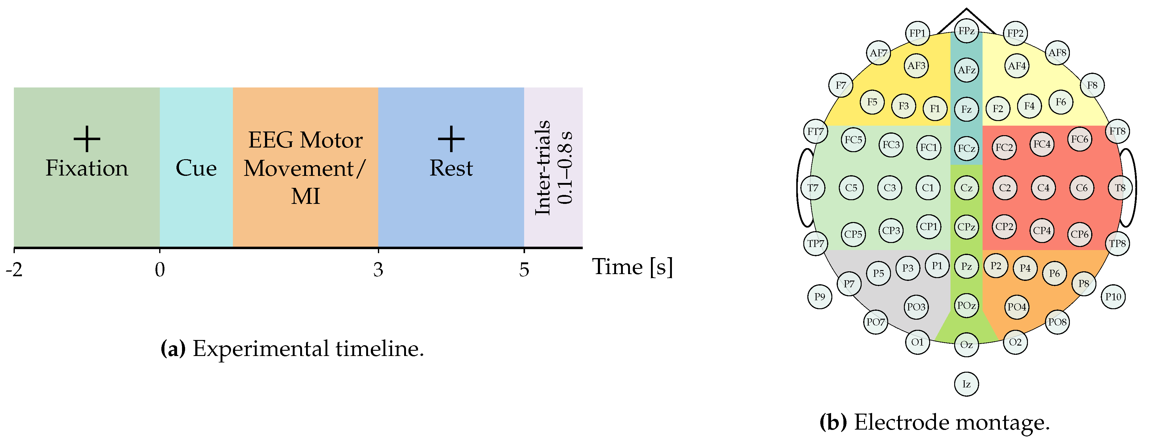
Figure 2.
The proposed EEG-GCIRNet framework, composed of two main stages: Top: A feature engineering pipeline that transforms raw EEG signals into multi-channel topographic maps using GFC. Bottom: A VAE architecture that processes these maps to jointly learn reconstruction, classification, and regularization from a shared latent space.
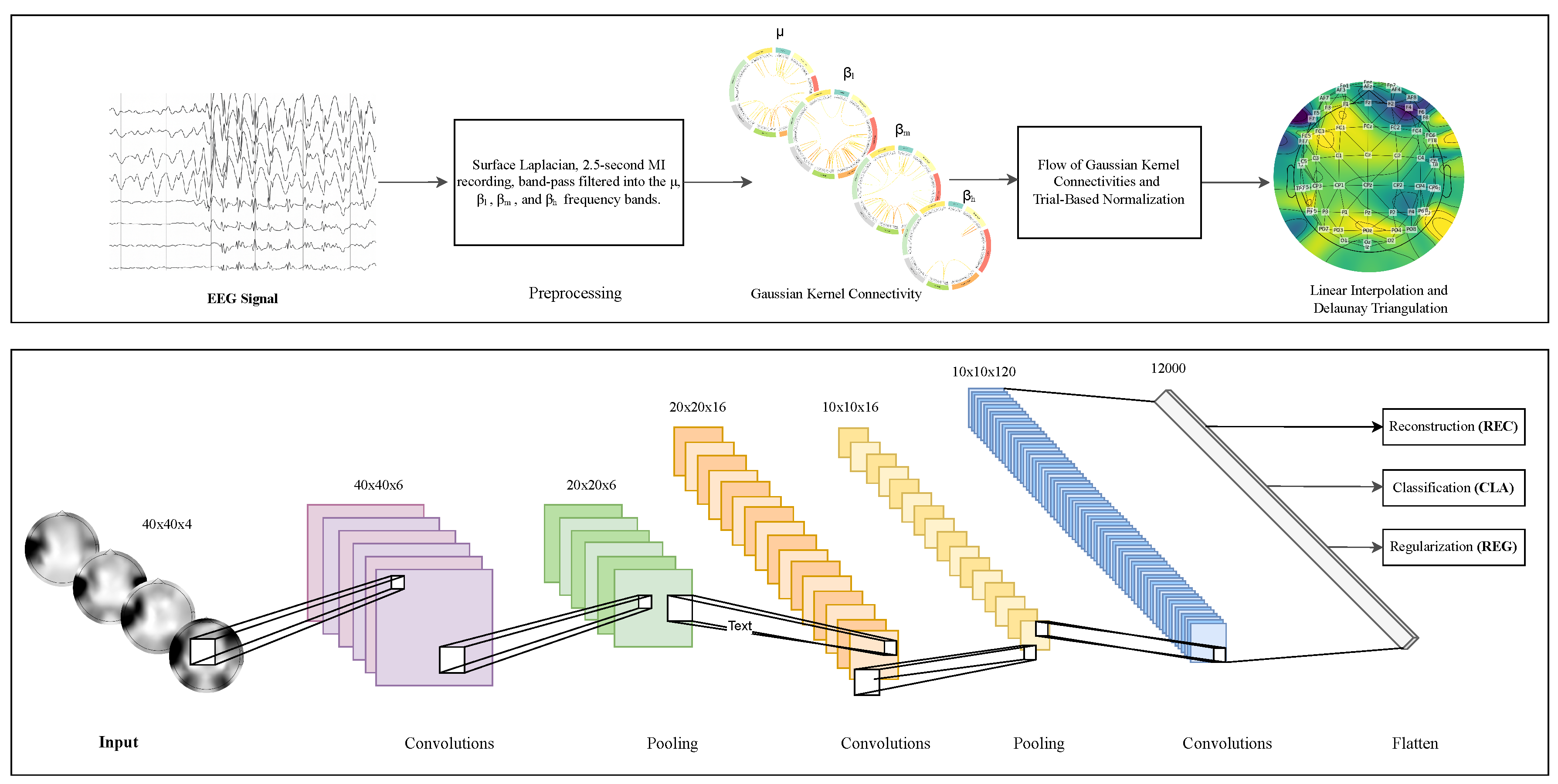
Figure 3.
Inter-subject accuracies results. Subjects are sorted based on EEGNet performance.
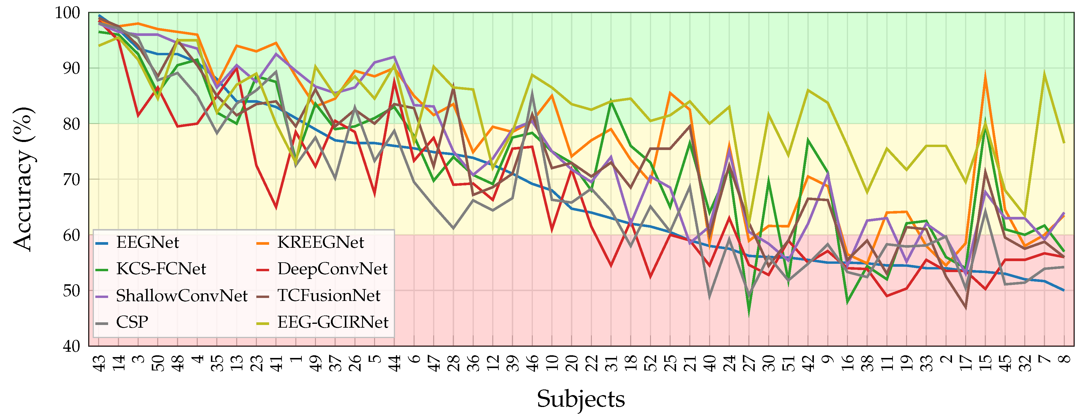
Figure 4.
Models rankings vs. t-test p-values. Subjects are sorted based on EEGNet’s accuracy.
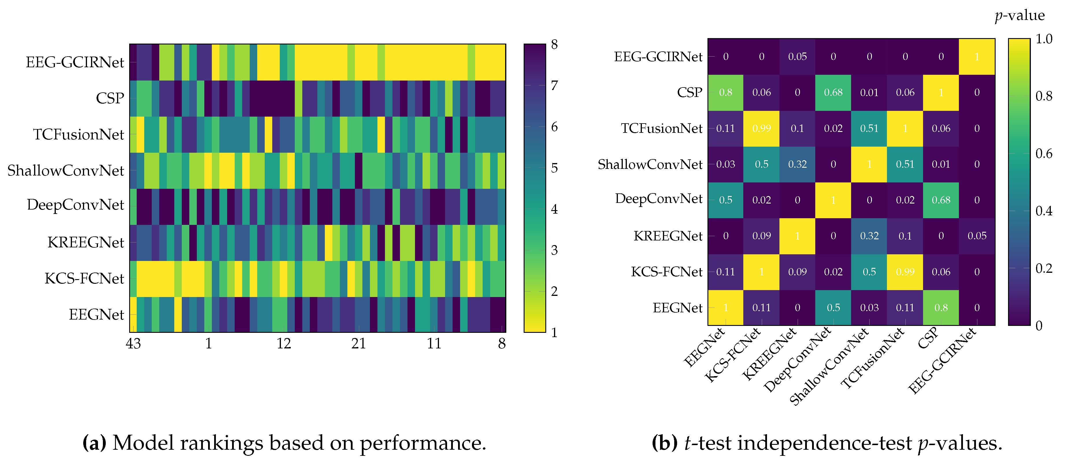
Figure 5.
Group performing MI-EEG classification results.
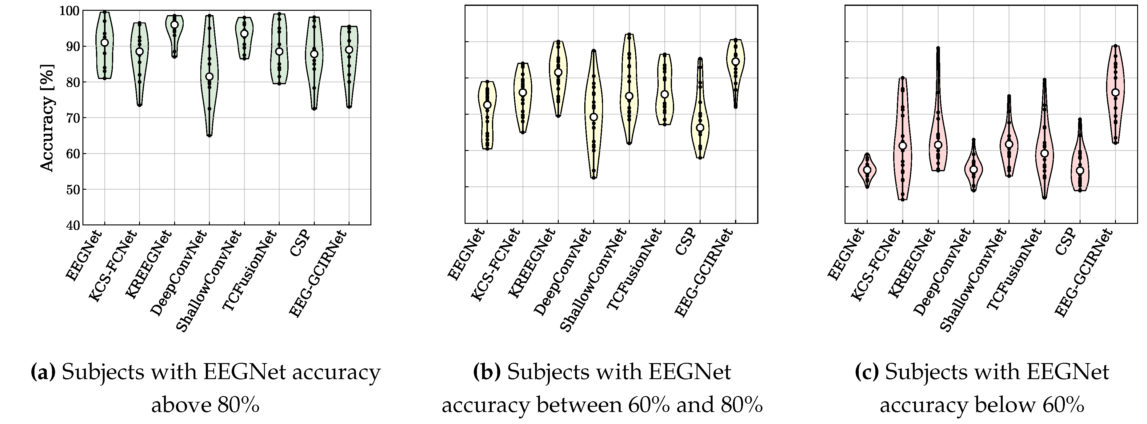
Figure 6.
Inter-subject classification accuracies of EEGNet and EEG-GCIRNet. Each bar represents the average performance per subject, with subjects ordered according to EEGNet accuracy to highlight the comparative improvements achieved by EEG-GCIRNet. Error bars indicate performance variability.
Figure 6.
Inter-subject classification accuracies of EEGNet and EEG-GCIRNet. Each bar represents the average performance per subject, with subjects ordered according to EEGNet accuracy to highlight the comparative improvements achieved by EEG-GCIRNet. Error bars indicate performance variability.
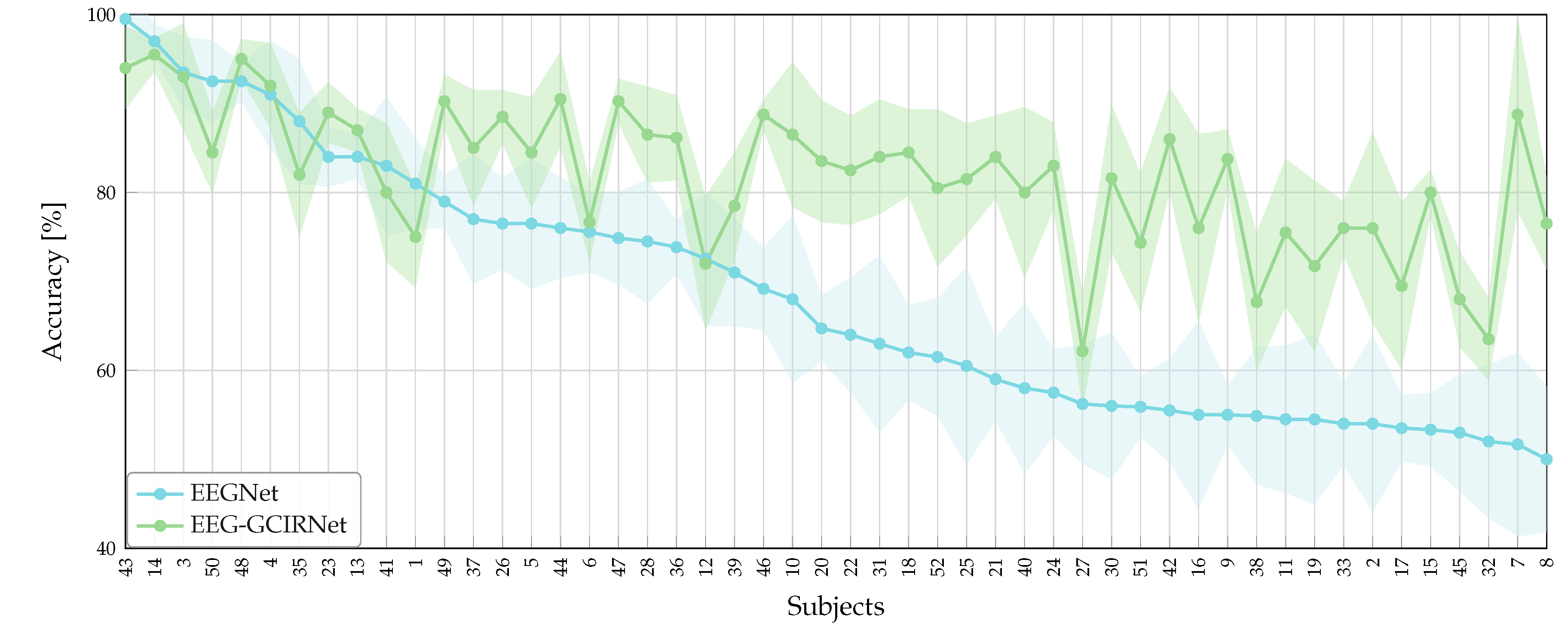
Figure 7.
Distributions of the weights corresponding to the three loss components—reconstruction (REC), classification (CLA), and latent space regularization (REG)—for the performance groups good and mid.
Figure 7.
Distributions of the weights corresponding to the three loss components—reconstruction (REC), classification (CLA), and latent space regularization (REG)—for the performance groups good and mid.
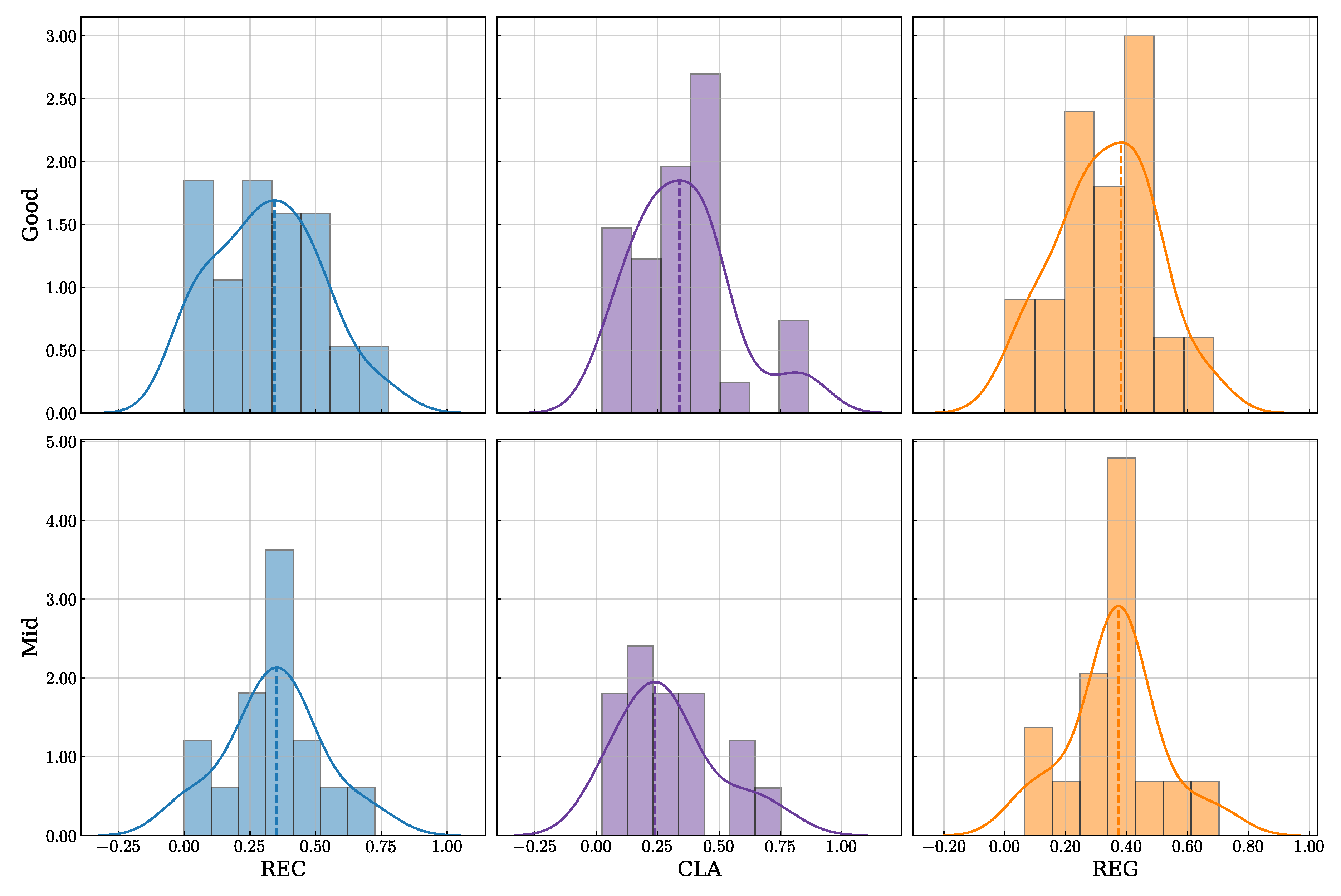
Figure 8.
Reconstruction subject 14 corresponding to group “Good”.
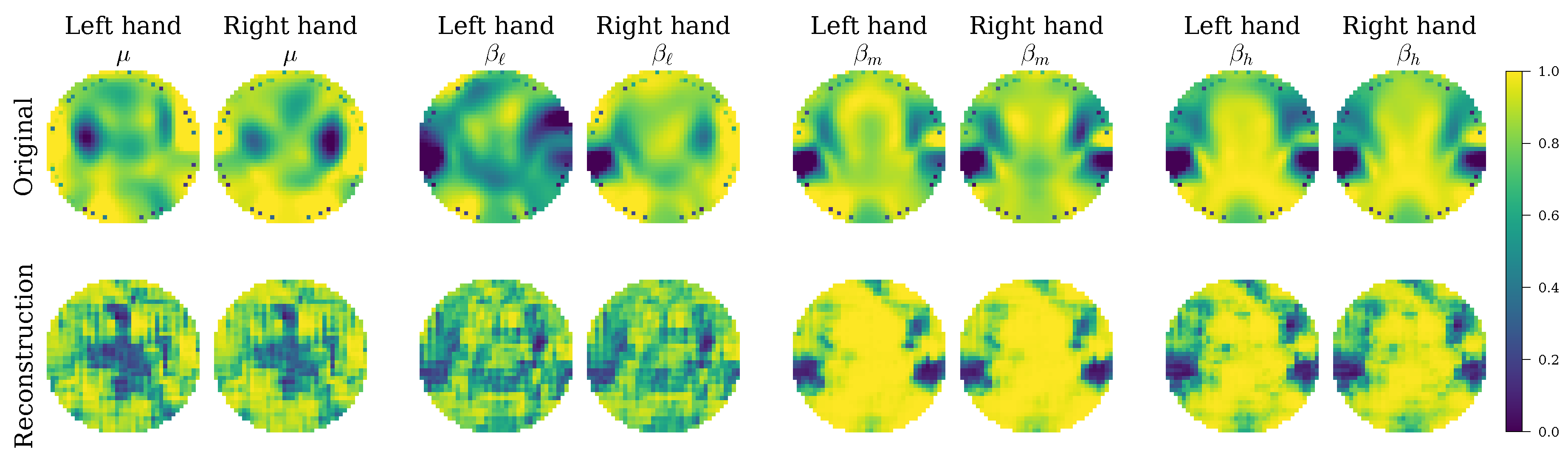
Figure 9.
Reconstruction subject 27 representing group “Mid”.
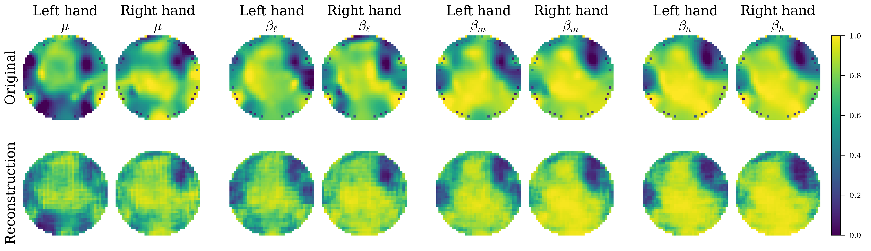
Figure 10.
t-SNE of Latent Representations by Performance Group good, mid
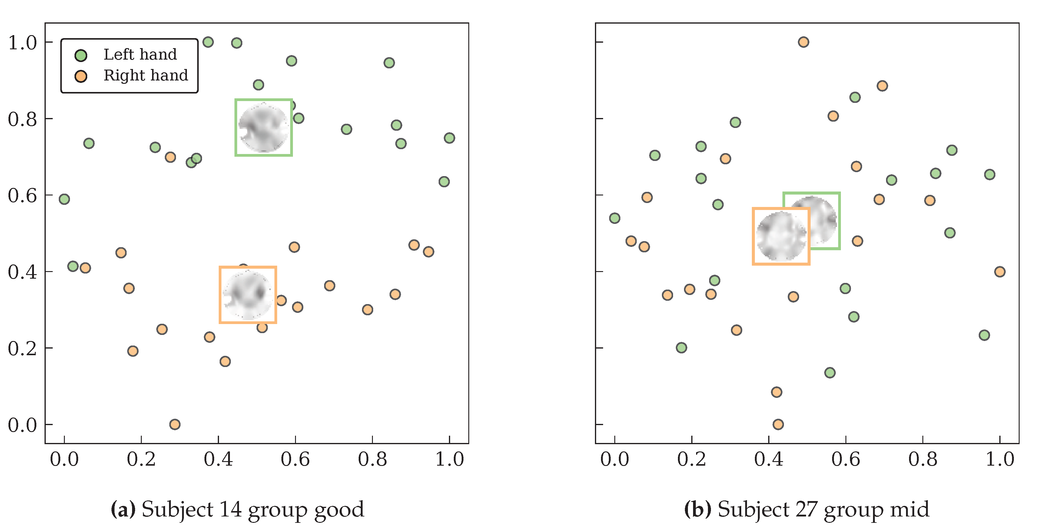

Table 1.
Layer-wise configuration of the EEG-GCIRNet architecture. The input shape corresponds to the four-channel topographic maps ().
Table 1.
Layer-wise configuration of the EEG-GCIRNet architecture. The input shape corresponds to the four-channel topographic maps ().
| Block | Layer | Kernel/Units | Strides | Activation | Output Shape |
|---|---|---|---|---|---|
| Input Image | |||||
| Encoder | Conv2D | , 6 Filters | SELU | ||
| () | AvgPool2D | - | |||
| Conv2D | , 16 Filters | SELU | |||
| AvgPool2D | - | ||||
| Conv2D | , 120 Filters | SELU | |||
| Flatten | - | - | - | ||
| Dense | 128 Units | - | SELU | ||
| Latent Space | Dense () | 128 Units | - | Linear | |
| (Reparameterization) | Dense () | 128 Units | - | Linear | |
| Decoder | Dense | 128 Units | - | SELU | |
| () | Dense | 12000 Units | - | SELU | |
| Reshape | - | - | |||
| Conv2DTranspose | , 16 Filters | SELU | |||
| Upsampling | - | ||||
| Conv2DTranspose | , 6 Filters | SELU | |||
| Upsampling | - | ||||
| Reconstruction | - | Sigmoid | |||
| Classifier | Dense | 128 Units | - | SELU | |
| () | Dense (Output) | 2 Units | - | Softmax | |
Table 2.
MI-EEG classification performance comparison: Average ACC (± standard deviation).
| Model | ACC |
|---|---|
| CSP [20] | |
| EEGNet [50] | |
| KREEGNet [44] | |
| KCS-FCNet [38] | |
| DeepConvNet [51] | |
| ShallowConvNet [52] | |
| TCFusionNet [53] | |
| EEG-GCIRNet (Our) |
Table 3.
Average rankings and p-values
| Model | Avg. Ranking | Avg. T-test p-value |
|---|---|---|
| CSP | ||
| EEGNet | ||
| KCS-FCNet | ||
| KREEGNet | ||
| DeepConvNet | ||
| ShallowConvNet | ||
| TCFusionNet | ||
| EEG-GCIRNet |
Table 4.
Accuracy and Gain by Group and Approach
| Approach | Group | Accuracy (%) | Gain (%) |
|---|---|---|---|
| EEGNet | Good | 89.64 | – |
| Mid | 70.54 | – | |
| Bad | 54.65 | – | |
| EEG-GCIRNet | Good | 87.86 | |
| Mid | 84.24 | ||
| Bad | 76.20 |
Disclaimer/Publisher’s Note: The statements, opinions and data contained in all publications are solely those of the individual author(s) and contributor(s) and not of MDPI and/or the editor(s). MDPI and/or the editor(s) disclaim responsibility for any injury to people or property resulting from any ideas, methods, instructions or products referred to in the content. |
© 2025 by the authors. Licensee MDPI, Basel, Switzerland. This article is an open access article distributed under the terms and conditions of the Creative Commons Attribution (CC BY) license (http://creativecommons.org/licenses/by/4.0/).
Copyright: This open access article is published under a Creative Commons CC BY 4.0 license, which permit the free download, distribution, and reuse, provided that the author and preprint are cited in any reuse.


