
Submitted:
05 June 2025
Posted:
11 June 2025
You are already at the latest version
Abstract
Motor Imagery (MI) classification plays a crucial role in enhancing the performance of brain-computer interface (BCI) systems, thereby enabling advanced neurorehabilitation and the development of intuitive brain-controlled technologies. However, MI classification using electroencephalography (EEG) is hindered by spatiotemporal variability and the limited interpretability of deep learning (DL) models. To mitigate these challenges, Dropout techniques are employed as regularization strategies. Nevertheless, the removal of critical EEG channels, particularly those from the sensorimotor cortex can result in substantial spatial information loss, especially under conditions of limited training data. This issue, compounded by high EEG variability in subjects with poor performance, hinders generalization and reduces the interpretability and clinical trust in MI-based BCI systems. This study proposes a novel framework integrating channel dropout—a variant of Monte Carlo Dropout (MCD)—with Class Activation Maps (CAMs) to enhance robustness and interpretability in MI classification. This integration represents a significant step forward by offering, for the first time, a dedicated solution to concurrently mitigate spatiotemporal uncertainty and provide fine-grained neurophysiologically relevant interpretability in motor imagery classification, particularly demonstrating refined spatial attention in challenging low-performing subjects. We evaluate three DL architectures (ShallowConvNet, EEGNet, TCNet Fusion) on a 52-subject MI-EEG dataset, applying channel dropout to simulate structural variability and LayerCAM to visualize spatiotemporal patterns. Results demonstrate that among the three evaluated deep learning models for MI-EEG classification, TCNet Fusion achieved the highest peak accuracy of 74.4% using 32 EEG channels. At the same time, ShallowConvNet recorded the lowest peak at 72.7%, indicating TCNet Fusion’s robustness in moderate-density montages. Incorporating MCD notably improved model consistency and classification accuracy, especially in low-performing subjects where baseline accuracies were below 70%; EEGNet and TCNet Fusion showed accuracy improvements of up to 10% compared to their non-MCD versions. Furthermore, LayerCAM visualizations enhanced with MCD transformed diffuse spatial activation patterns into more focused and interpretable topographies, aligning more closely with known motor-related brain regions and thereby boosting both interpretability and classification reliability across varying subject performance levels. Our approach offers a unified solution for uncertainty-aware, and interpretable MI classification.
Keywords:
Motor Imagery
; Channel Dropout
; Class Activation Maps
; Spatiotemporal Uncertainty
1. Introduction
Motor imagery (MI) involves the mental simulation of motor actions without physical movement, engaging neural circuits similar to those activated during execution [1]. This cognitive process underpins MI-based brain-computer interfaces (BCIs), which translate neural activity into control signals for external devices, with applications in neurorehabilitation and assistive technologies [2]. MI classification using deep learning (DL) models is a cornerstone of BCI research, offering advancements over classical techniques. However, several challenges impede robust system development. Spatiotemporal uncertainty arises from EEG signal variability, limited datasets (often fewer than 50 subjects [3]), and inter-subject heterogeneity [4]. The high dimensionality and noise of EEG data complicate feature extraction and training, often leading to overfitting and requiring architectures that balance complexity with generalizability [5,6]. Additionally, practical considerations like channel configurations impact performance: lower channel counts enhance portability but may reduce accuracy and stability [7,8]. The black-box nature of DL models further hinders understanding of learned representations, necessitating interpretable solutions for reliable real-world applications [9,10].
In response to these montage variability challenges, channel dropout has emerged as a promising solution. As a variant of Monte Carlo Dropout (MCD), it addresses montage variability by randomly disabling EEG channels during training and inference, enhancing robustness and generalization [11]. However, its effectiveness is limited by persistent overfitting due to scarce data and high intra- and inter-subject variability [12], as well as architecture-specific dropout tuning and computational costs that hinder real-time deployment [13]. To overcome these limitations, researchers have turned to Class Activation Maps (CAMs), particularly LayerCAM, which visually highlight key spatial and temporal features driving classification [14]. Integrating channel dropout with CAMs offers a synergistic approach, where dropout boosts robustness and CAMs refine interpretations of critical channels and dynamics, especially in low signal-to-noise ratio or sparse montage scenarios [15].
However, the ultimate challenge that both channel dropout and CAMs must collectively address is the substantial subject variability that characterizes MI-based BCI systems. This variability manifests through differences in brain anatomy, cognitive strategies, and neural response patterns, creating a complex landscape where the non-stationarity and inherent variability of EEG signals across subjects obscure physiologically meaningful spatiotemporal features [16]. Consequently, diffuse activations complicate identifying task-relevant cortical regions, such as the primary motor cortex, while montage variability and limited resolution hinder generalization. Traditional methods like Common Spatial Patterns (CSP) offer interpretability but are sensitive to noise and session variability [17].
To address this multi-faceted challenge of subject variability, the combined application of channel dropout and CAMs offers a more comprehensive solution than either approach in isolation. By providing robust feature extraction through channel dropout while maintaining interpretability through CAM visualization, this integrated approach enables researchers to understand how different subjects engage distinct neural patterns during MI tasks. This understanding proves crucial for developing subject-specific adaptations and optimized montage designs that ensure reliable classification across diverse user populations. Recent explainable AI approaches have further enhanced this integration by leveraging spectral and spatial features, validated against neurophysiological data, to balance performance and interpretability [18]. Additionally, hybrid regularization techniques that integrate dropout with batch normalization and data augmentation offer additional pathways for improvement, emphasizing the need for adaptive, subject-aware tuning to ensure robust MI classification [19]. Despite these promising developments, the combined use of channel dropout and CAM to address spatiotemporal uncertainty in MI classification remains underexplored, particularly in low-performing subjects where interpretability becomes critical for practical BCI deployment. Moving forward, this integrated approach represents a unified framework for achieving robust, interpretable MI classification that effectively addresses the interconnected challenges of spatiotemporal uncertainty, montage variability, and subject heterogeneity in real-world BCI applications.
This paper proposes a novel uncertainty-aware deep learning framework for MI-EEG classification, aiming to simultaneously enhance model robustness and interpretability, particularly in low-performing subjects. In this sense, a channel-wise Monte Carlo Dropout (MCD) and LayerCAM-based spatial interpretability are integrated, a combination not previously explored in the MI-EEG domain. This unified framework enables the dynamic modeling of spatiotemporal uncertainty and yields neurophysiologically meaningful insights by refining spatial attention patterns. Regarding this, our proposal is structured around four major methodological stages:
- Channel Dropout Regularization: Introducing structural noise to simulate montage variability and improve generalization.
- LayerCAM Integration: Enhancing model transparency by visualizing discriminative EEG regions per MI class.
- Evaluation Across Varying Montages: Testing 8, 16, 32, and 64-channel configurations to assess robustness and practical applicability.
- Performance Analysis by Subject Grouping: Stratifying subjects into high- and low-performing cohorts to investigate model behavior across heterogeneous EEG data.
Experiments are conducted using a 52-subject GigaScience MI-EEG dataset and involve three deep learning models (ShallowConvNet, EEGNet, and TCNet Fusion) with and without MCD. Results show that TCNet Fusion achieves the best overall performance, while EEGNet demonstrates the highest generalizability, especially when paired with optimally tuned dropout rates. The integration of MCD and LayerCAM consistently transforms diffuse activation patterns into focused, interpretable topographies across subject types, enhancing both performance and reliability. Therefore, our channel-wise MCD combined with LayerCAM represents a scalable and interpretable approach to tackle spatiotemporal uncertainty and subject variability in MI-BCI systems.
The remainder of this paper is organized as follows: Section 2 details the methods, including baseline feature extraction with FBCSP and the implementation of three DL models (ShallowConvNet, EEGNet, and TCNet Fusion) tailored to EEG signal characteristics, alongside channel dropout and CAM integration. Section 3 outlines the experimental setup, covering the MI-EEG dataset, preprocessing, montage reduction, and evaluation metrics for robustness and interpretability across subject groups. Section 4 presents results and discussion, analyzing classification accuracy, dropout effects on stability, and LayerCAM-based spatiotemporal patterns. Finally, Section 5 concludes with key findings and future directions for uncertainty-aware MI classification.
2. Materials and Methods
Baseline Feature Extraction of Spatiotemporal Characteristics
Given a dataset composed by , consisting of EEG trials—where C denotes the number of channels and T the number of temporal samples per trial—the classification task aims to learn a function that predicts the binary label (), corresponding to the brain’s neural responses to left- and right-hand MI, respectively.
As a classical baseline, we include the Filter Bank Common Spatial Pattern (FBCSP) method, widely used in MI-BCI systems for its effectiveness in extracting subject-specific spatio-spectral features. The baseline MI binary classification approach involves spatial filtering via linear transformations of the EEG data to enhance class separability—specifically, by maximizing the variance of signals associated with one class while minimizing it for the other [20,21]. The EEG signals are first passed through a filter bank comprising bandpass filters, typically centered on canonical sub-bands (e.g., mu, alpha, beta) or custom frequency ranges. This process yields filtered EEG segments . Following the FBCSP procedure [22], features are extracted by computing the log-variance of the spatially filtered signals , as given by:
where extracts the diagonal elements of the covariance matrix, denotes the trace operator, and represents the spatially filtered signal using projection matrix , which contains the most discriminative spatial filters for sub-band .
Deep Learning Frameworks for Feature Extraction of MI Responses
Building upon the baseline FBCSP approach, we consider three well-established DL architectures, each specifically designed to address the unique spatiotemporal characteristics of EEG signals in MI classification. These models have demonstrated competitive performance and complementary strengths in recent EEG-based BCI benchmarks [23], providing a comprehensive foundation for evaluating the effectiveness of our proposed channel dropout and CAM integration approach.
- ∗
- ∗
- EEGNet Framework. In this architecture, feature extraction is carried out through a sequence of convolutional blocks , structured as [25]:where and denote the number of temporal and separable filters, respectively; and are the kernel sizes for the temporal and depthwise convolutions; and is the number of spatial filters. Each block is followed by batch normalization and non-linear activation.
- ∗
- TCNet (Temporal Convolutional Network) Framework. TCNet extends the prior architectures by integrating temporal convolutional modules with residual connections [26,27]. The model combines filter bank design with deep temporal processing through the sequential application of blocks , as follows:where and are the kernel sizes for the initial and filter bank convolutions, is the number of feature maps, L is the number of residual blocks, , and denotes a temporal convolutional block with dilated convolutions. The dilation factor increases with l, enabling exponential growth in the receptive field while preserving temporal resolution.
The final classification stage in all three DL frameworks is performed by a fully connected layer applied to the flattened output of the last feature extraction layer , with the classification computed as:
where denotes the class probability distribution over K classes. In this expression, is the d-dimensional feature vector obtained by applying global average pooling to the final convolutional feature maps. The matrix contains the weights of the fully connected layer, and represents the corresponding bias vector.
Monte Carlo Dropout with CAM Integration for MI Classification
To address the limitations of traditional approaches and enhance both robustness and interpretability in EEG-based MI classification, we integrate Monte Carlo Dropout (MCD) with Class Activation Maps (CAMs) across the deep learning architectures described above [28]. This integration provides a unified framework that simultaneously quantifies prediction uncertainty and visualizes spatiotemporal patterns critical for MI classification.
Channel dropout is applied by introducing a dropout mask component-wise to the input EEG tensor , such that the modified input becomes , where ⊙ denotes element-wise multiplication. For a given layer output , the MCD operation is defined as:
where is the dropout probability, is a random mask vector sampled from a Bernoulli distribution with success probability . The scaling factor preserves the expected activation magnitude, ensuring .
During inference, MCD generates T stochastic predictions, which are then augmented by CAMs to visualize spatially relevant features. This integration is formalized as [29]:
where is the network with dropout mask , is the prediction vector, is the final output, and quantifies uncertainty. For CAM computation, is the activation map for class c, is the activation of unit k in the target layer, and is the importance weight averaged over T MCD samples, normalized by Z (number of spatial locations), with gradients reflecting feature relevance.
3. Experimental Set-Up
Evaluating Framework
This study proposes a channel-wise dropout-based framework augmented with CAMs to enhance the interpretability of neural network decisions. The framework dynamically identifies spatial (channel-level) contributions that vary temporally and may contribute to misclassifications in MI-evoked brain responses.
As shown in Figure 1, the framework comprises the following stages:
- ∗
- Data Preprocessing and Montage Reduction. We evaluate the impact of EEG montage size on model generalizability, hypothesizing that excessive channels promote overfitting on spatially correlated artifacts rather than task-specific MI neural dynamics. Montage sizes are tested separately for the best- and worst-performing subjects. Subjects are stratified into high (best)- and low (worst)-performance cohorts based on evaluated trial accuracy ( or). This serves as a conventional reference for evaluating the benefits of DL-based frameworks in ranking subjects based on their trial-level classification accuracy.
- ∗
- Subject Grouping Based on the Classification Accuracy of MI Responses. We evaluate three Neural network models for EEG-based classification, EEGNet and ShallowConvNet, for their real-time applicability, alongside the advanced TCNet Fusion architecture for enhanced performance. As stated above, we use FBCSP as a classical baseline for extracting subject-specific spatio-spectral features. This provides a conventional reference to assess the benefits of deep learning-based approaches.
- ∗
- Spatio-temporal uncertainty estimation. MCD is applied to assess each model’s ability to learn robust, channel-independent features, thereby reducing overfitting and improving generalization. Furthermore, MCD is combined with CAMs to estimate spatio-temporal uncertainty and enhance model interpretability. Specifically, the variance computed across CAMs is overlaid onto the original CAM representation, highlighting regions where the model exhibits reduced certainty in its interpretation of MI responses.
Motor Imagery EEG Data Collection. For validation purposes, we utilize an electroencephalogram dataset from MI-based brain–computer interface experiments, comprising data from 52 healthy participants (mean age: years)1. Of note, subjects labeled as 29, 32, 34, 46, and 49 were excluded because their data lacked sufficient discriminative power, a practice also followed in [17].
The experimental protocol requires participants to imagine left- and right-hand movements in response to standardized visual cues displayed on a screen. EEG signals are recorded using a 64-channel Biosemi ActiveTwo system at a sampling rate of 512 Hz. Additionally, simultaneous electromyographic recordings are conducted to ensure the absence of actual hand movements during MI trials. The experimental paradigm, illustrated in Figure 2, follows a structured MI task designed to elicit EEG data corresponding to imagined left- and right-hand movements. Participants are seated comfortably with armrests and positioned facing a monitor on which visual cues are displayed. Each trial begins with a black screen and a fixation cross for 2 s to allow for task preparation. This is followed by a visual instruction—either “Left hand” or “Right hand”—presented for 3 s, prompting participants to imagine sequential finger movements corresponding to the indicated hand. Afterward, a blank screen is displayed for a randomized interval of 4.1 to 4.8 s, serving as a rest period and reducing task predictability. Note that the protocol emphasizes kinesthetic experience of movement (i.e., the sensation of muscle activation), rather than visual imagery.
All participants completed five to six runs per session, with each run consisting of 100–120 trials per MI class. Each trial is carefully structured to ensure consistency in data collection, as participants follow standardized visual cues to perform the MI task. Trials are evenly distributed between left- and right-hand imagery conditions, yielding a balanced dataset for analysis.
Additionally, feedback is provided after each run to enhance participant engagement. This dataset enables robust validation through event-related desynchronization/synchronization analysis, classification accuracy metrics, and identification of noisy or artifact-contaminated trials. The comprehensive experimental design serves as a valuable resource for studying performance variability in MI-BCI systems and for developing subject-independent models.
EEG Preprocessing and Reduction of EEG-Channel Montage Set-Up
The collected EEG signals are preprocessed prior to training to ensure high data quality. First, an average reference is applied and then re-referenced to include the original reference electrode, thereby preserving the full rank of the data [30]. A fifth-order Butterworth bandpass filter (4–40 Hz) is subsequently applied to isolate the relevant frequency range, as suggested in [31]. Since the dataset focuses on motor imagery rather than higher-order cognitive processes such as multisensory integration, the analysis targets three primary frequency bands: Theta (4–8 Hz), Alpha (8–13 Hz), and Beta (13–32 Hz) [32]. The Gamma band (above 40 Hz) is excluded, as it is typically not informative for MI-based tasks [33].
To standardize the input across deep learning models, the signals are downsampled from 512 Hz to 128 Hz, in line with the recommendations in [34]. Finally, to enhance the physiological relevance of the analysis, only the MI time window between 0.5 and 3 s is selected for detailed evaluation.
To assess the consistency of DL model performance across subjects, the preprocessed EEG signals are configured into four electrode montages: 8-, 16-, 32-, and 64-channel configurations. The spatial configurations of the channel montages used for multichannel EEG acquisition are shown in Figure 3.
Evaluated Deep Learning Models for EEG-based Classification
For evaluation, we consider three well-established DL models, each recognized for their specialized architectures tailored to EEG signal analysis. These models are designed to ensure efficient feature extraction, robustness, and adaptability in MI tasks [35]. Figure 4 provides a concise visual overview of the evaluated MI-EEG architectures:
- ∗
- ShallowConvNet [36]: A low-complexity architecture that emphasizes early-stage feature extraction through sequential convolutional layers, square and logarithmic nonlinearities, and pooling operations. It effectively emulates the principles of the classical FBCSP pipeline within an end-to-end trainable deep learning framework, offering robust performance in MI classification tasks.
- ∗
- EEGNet [25]: A compact, parameter-efficient model that utilizes depthwise and separable convolutions to disentangle spatial and temporal features. Designed for cross-subject generalization and computational efficiency, EEGNet maintains competitive accuracy across a wide range of EEG-based paradigms.
- ∗
- TCNet Fusion [37]: A high-capacity architecture that incorporates residual connections, dilated convolutions, and convolutions to construct a multi-pathway fusion network. Its hierarchical design captures long-range temporal dependencies and enhances feature integration across time, improving classification performance in complex MI scenarios.
As noted previously, an additional methodological consideration involves ranking subjects in descending order based on their individual classification accuracy. Since each deep learning model yields a different subject-wise ranking, the ordering derived from the classical feature extraction method FBCSP is adopted as a consistent baseline reference for comparative performance evaluation.
Subject Grouping Based on the Classification Accuracy of MI Responses
To assess model robustness and quantify predictive uncertainty, we integrate MCD into the evaluated DL architectures referred to as (e.g., MCD-EEGNet) [11]. MCD enables uncertainty estimation by simulating multiple stochastic forward passes through the network during inference. This approach provides a more reliable evaluation of model behavior under variable conditions, such as the presence of defective channels during EEG acquisition, thereby enhancing the reliability of predictions. Specifically, we implement MCD by introducing a dropout layer prior to the first Conv2D layer. This layer applies a binary dropout mask to the multi-channel EEG input, randomly disabling channels over time to simulate structural variability and improve generalization.
To interpret the elicited brain activity, we consider the influence of BCI illiteracy [38], which suggests that classification frameworks may fail to accurately decode brain responses from certain individuals, resulting in poor performance. To address this issue, we cluster subjects based on inter-subject variability in neural responses, grouping individuals with similar classification accuracies.
The rationale behind this grouping is that classification performance may reflect an individual’s ability to engage in MI tasks: the more accurately a subject distinguishes between MI conditions, the more effectively their brain network may be functioning during the task. For evaluation, we order the individuals by accuracy, defining two groups:
- ∗
- Group I: Well-performing subjects with binary classification accuracy above 70%, as proposed in [39].
- ∗
- Group II: Poor-performing subjects with accuracy below this threshold.
As the performance measure, classifier accuracy is computed as:
where , , , and denote true positives, true negatives, false positives, and false negatives, respectively.
To assess performance beyond random chance, the Cohen’s kappa coefficient is also calculated as:
where for binary classification problems.
For validation, the training trial set is randomly partitioned using stratified 10-fold cross-validation. This procedure is repeated ten times, each time rotating the test and training subsets to ensure stability and generalizability of the reported performance metrics.
Enhanced CAM-Based Spatial Interpretability
We compute Layer-wise Class Activation Maps (Layer-CAM), a technique designed to enhance the interpretability of neural network decisions [40]. This method generates heatmaps that highlight the most relevant regions of the input, providing insights into the model’s focus during classification. Unlike traditional CAM approaches, Layer-CAM identifies class-discriminative regions at intermediate layers, offering a multilevel perspective on feature importance. Additionally, it facilitates model refinement by localizing misinterpreted regions, thereby supporting targeted performance improvements.
According to Equation 1, The MCD-enhanced model (MCD-EEGNet) apply dropout after convolutional layers, using rates optimized via cross-validation to ensure stable uncertainty estimates while maintaining computational efficiency [41]. CAMs are computed with samples to stabilize weight estimates , providing interpretable spatial attention maps for MI tasks. This approach leverages recent advancements in uncertainty estimation and feature visualization, offering insights into brain activity patterns and supporting reliable classification, especially for subjects with variable performance. For each model, the activation maps are extracted from the first temporal convolutional layer. This choice is motivated by the architectural design in which spatial convolutions are subsequently applied in the second convolutional stage, reducing the multi-channel EEG representation to a single channel. Extracting CAMs beyond this point would primarily emphasize temporal dynamics, thereby limiting spatial interpretability. By targeting the first convolutional stage, the resulting Layer-CAMs preserve relevant spatiotemporal information, enabling more interpretable analyses of neural representations.
To ensure consistency and reproducibility, all DL models are implemented using the high-level Keras API (version 3.2.1) within the TensorFlow framework (version 2.17.0). Each model is trained for a maximum of 500 epochs, with early stopping triggered in the presence of NaN values. A learning rate reduction scheduler is employed to adaptively adjust learning when performance plateaus. The Adam optimizer is used alongside categorical cross-entropy as the loss function. Unless otherwise specified, all hyperparameters follow TensorFlow’s default settings, and each model is trained in accordance with its original implementation. Model evaluation is performed using five-fold stratified cross-validation, and the best-performing model for each subject is selected based on classification accuracy.
4. Results and Discussion
Tuning of validated DL models
To assess the relative performance of the proposed approaches, we conducted a comprehensive comparison against three convolutional neural network (CNN)-based deep learning models widely adopted in the literature. These include established architectures such as ShallowConvNet, EEGNet, and advanced variants like TCNet Fusion. Performance was evaluated using standard metrics—accuracy, kappa, and AUC—across a unified experimental protocol using the GigaScience MI-EEG dataset, as shown in Figure 5.
As seen, TCNet Fusion[37] achieved the highest performance, attaining the top metric value with relatively low variability. This result indicates not only strong predictive capability but also consistent behavior across evaluation runs. EEGNet[25] ranked second, delivering solid performance accompanied by moderate dispersion. In contrast, ShallowConvNet[24] recorded the lowest performance and exhibited the highest variability, suggesting it is both less effective and less reliable for the given task. The use of Monte Carlo Dropout led to performance improvements across all models reducing performance variability, with MCD TCNet Fusion achieving the best overall results in both accuracy and stability. MCD EEGNet also showed notable gains, while MCD ShallowConvNet exhibited only slight improvement and remained the weakest model. Thus, MCD consistently enhanced both predictive accuracy and reliability, particularly in models with stronger baseline performance.
Accuracy of MI Responses: Results of Subject Grouping
In our approach, we leverage channel-montage reduction to enhance validation reliability by balancing classification accuracy and inter-subject consistency under the practical constraints of each evaluated deep learning model. Table 1 reports the average classification accuracy across various channel configurations, enabling a comparative performance analysis. Notably, all three models improve with increasing electrode count up to 32 channels. TCNet Fusion attains its peak accuracy (0.744) at 32 channels, slightly outperforming its performance at 64 channels (0.739). Likewise, EEGNet and ShallowConvNet reach peak accuracies of 0.737 and 0.727, respectively, also at 32 channels. These trends suggest that reducing from 64 to 32 channels may enhance performance by mitigating the effects of noisy or redundant electrodes.
In terms of model-specific robustness to channel reduction from 32 to 8 channels, TCNet Fusion demonstrates a high degree of stability, maintaining accuracy within the range of 0.700–0.744, corresponding to a relative drop of only 4.4%. EEGNet exhibits a slightly smaller decline of 3.1% (from 0.737 to 0.706), while ShallowConvNet shows the smallest reduction in accuracy (2.7%) but also records the lowest peak performance (0.727). These findings suggest that the architectural complexity of TCNet Fusion, and to a lesser extent EEGNet, provides greater adaptability to sparse montage configurations compared to simpler models such as ShallowConvNet.
The boxplot in Figure 6 supports this, showing that TCNet Fusion achieves an accuracy of 0.729 with 16 channels, representing a mere 2% drop from its peak performance at 32 channels. Similarly, both EEGNet and ShallowConvNet retain more than 95% of their respective peak accuracies at this reduced configuration. These results imply that halving the number of channels—from 32 to 16—leads to only marginal performance degradation. Consequently, 16-channel setups are a practical choice for portable EEG systems, offering a favorable trade-off between hardware simplicity and classification performance.
Another important consideration is inter-model consistency, evaluated through accuracy variability across DL models. At 32 channels, the performance gap between the best model (TCNet Fusion: 0.744) and the worst-performing model (ShallowConvNet: 0.727) is 2.3%. However, when the number of channels is reduced to 8, this gap narrows to just 1.1% (TCNet Fusion: 0.700 vs. ShallowConvNet: 0.708), indicating that sparse montages (8–16 channels) reduce inter-model variability. That is, montage reduction can enhance practical usability without sacrificing accuracy. Moreover, these results suggest that simpler models may suffice for low-channel configurations, whereas more advanced architectures, such as TCNet Fusion, are better suited for moderate- to high-density setups—up to at least 32 channels. Beyond this point, such as at 64 channels, model performance either remains comparable to the 32-channel setup or even degrades, with a noticeable increase in performance dispersion, regardless of the model architecture.
Figure 7 shows the EEG-based classification performance for each subject across the evaluated deep learning models. As previously noted, subjects are ranked according to their performance under the FBCSP method (indicated by the black line), which serves as a baseline grounded in traditional signal processing. This ranking facilitates a contextual interpretation of the performance gains achieved by deep learning approaches relative to a well-established conventional method.
As illustrated in Figure 7a (top row), the empirical results for ShallowConvNet—the first and most basic model evaluated—demonstrate that the EEG channel montage reduction strategy yields consistent classification accuracy across subjects. This consistency serves as an indicator of the model’s robustness, highlighting its generalizability across individuals. Nonetheless, substantial variability in performance is observed across different montage configurations, with the exception of subjects exhibiting markedly low classification efficacy.
For the next architecture, EEGNet—a structurally refined model relative to its predecessor—the empirical results depicted in Figure 7b (middle row) suggest a similar degree of consistency in classification performance across subjects. However, pronounced variability remains among subjects with notably low classification performance, indicating a limitation in robustness for this subgroup.
In contrast, the optimized TCNet Fusion architecture (Figure 7c, bottom row) exhibits superior inter-subject consistency, even among individuals with critically diminished classification accuracy. This result highlights the model’s resilience to variations in channel configuration and supports its effectiveness within the proposed DL framework.
A subject-wise comparison reveals several noteworthy patterns, as shown in Figure 8. For high-performing individuals (leftmost region), such as subjects 43, 14, and 3, classification accuracies remain consistently high across all models, with minimal variance. This implies that for subjects with well-defined discriminative EEG features, even simpler models (e.g., ShallowConvNet) can perform on par with more complex architectures. Moreover, deep learning models often underperform relative to the FBCSP baseline, suggesting that in these cases, brain response patterns are sufficiently strong and structured to be accurately captured by conventional signal processing techniques.
In the mid-range (e.g., subjects 22 through 15), the variability between models increases. For these individuals, TCNet Fusion frequently achieves the highest accuracy, while ShallowConvNet tends to underperform. As expected, the FBCSP baseline model in this range is often exceeded by the best-performing DL models, emphasizing the effectiveness of learned features in scenarios of moderate classification complexity. Notably, in mid-range and lower-performing subjects, TCNet often exceeds the accuracy of FBCSP and sometimes even EEGNet, further reinforcing the potential of temporal-convolutional modeling in moderately challenging contexts.
In contrast, for lower-performing individuals (rightmost subjects, such as 40, 27, and 42), accuracy values across all models decrease. However, dispersion among models becomes more apparent, and the performance gap between the best and worst models narrows. Interestingly, in several of these cases, FBCSP achieves accuracy values close to or better than some deep learning models, highlighting that for challenging subjects with weak class separability, handcrafted features may still offer competitive performance. Nonetheless, in low-performing subjects (right side of the plot), EEGNet often outperforms FBCSP, particularly where FBCSP falls below the 0.7 accuracy line, indicating its resilience in handling low signal quality scenarios.
Overall, the subject-wise analysis indicates that, compared to the baseline FBCSP approach, DL models—particularly TCNet Fusion—consistently outperform it for the majority of subjects (27 out of 43), especially those exhibiting moderate to high EEG signal quality. However, for approximately 30% of the subjects (17 out of 43), the use of any of the evaluated DL models results in a deterioration of classification accuracy relative to the FBCSP baseline. This suggests that the overall improvement across the entire cohort is achieved at the expense of high performance dispersion—where some individuals benefit substantially from DL models, while others experience significant performance degradation. Model Stability: EEGNet and TCNet show greater robustness across diverse subjects compared to FBCSP and shallow models, highlighting their superior adaptability to heterogeneous EEG characteristics. Such variability compromises the inter-model consistency and challenges the adaptability of these models to subject-specific EEG patterns.
Enhanced Consistency of DL Model Performance Using Monte Carlo Dropout
Figure 9 (first three rows) presents a comparative analysis of the effects of dropout regularization across multiple DL architectures, stratified by subject performance levels. This evaluation highlights key trends in model robustness and the role of regularization strategies in EEG-based MI classification tasks, while also facilitating uncertainty estimation to enhance model reliability, as discussed in [11]. In particular, the consistency of classification accuracy across varying Monte Carlo dropout rates serves as a critical indicator of each model’s resilience to regularization during inference.
Among the models examined, ShallowConvNet exhibits moderate stability. While it maintains relatively consistent performance for subjects in Group I—those with higher FBCSP baseline accuracies—more noticeable fluctuations emerge among subjects in Group II, where baseline performance is lower. These variations indicate a degree of sensitivity to the specific dropout rate applied. In contrast, EEGNet demonstrates improved stability, particularly within Group I, where accuracy values are more tightly clustered across dropout conditions. However, some variability remains in Group II, suggesting residual sensitivity in more challenging classification scenarios. Most notably, TCNet shows the highest degree of stability across all tested dropout rates. Its classification accuracy remains remarkably consistent across both subject groups, indicating a performance largely unaffected by changes in dropout rate and suggesting a more robust internal representation.
Beyond stability, overall classification accuracy and each model’s ability to outperform the FBCSP baseline are essential measures of effectiveness. ShallowConvNet yields competitive results, frequently surpassing the baseline for Group I subjects. However, this advantage tends to diminish in Group II, with several cases where performance falls below the FBCSP benchmark. EEGNet performs strongly in Group I, consistently achieving notable gains over the baseline. In Group II, its results are more variable—while it sometimes improves over the baseline, there are also instances where it fails to do so. In contrast, TCNet achieves the highest overall accuracy across the cohort and most consistently outperforms the FBCSP baseline. Accuracy levels in Group I often approach or exceed 0.9, and in Group II, TCNet typically maintains or modestly surpasses baseline performance. These results indicate a strong generalization capacity across varying levels of subject difficulty.
Regarding model generalizability, ShallowConvNet, while effective in Group I, shows diminished reliability in Group II, where it often fails to exceed the FBCSP baseline. EEGNet follows a similar trend, offering strong performance in Group I but delivering inconsistent results in Group II, with performance sometimes falling short of the baseline. In contrast, TCNet exhibits strong and consistent results across both groups. It maintains high performance in Group I while also producing stable and frequently improved outcomes in Group II, indicating an enhanced ability to extract discriminative features even from lower-quality EEG signals.
The comparative analysis clearly identifies TCNet as the most robust and consistent model across all evaluated dimensions. Its classification performance is highly stable under varying Monte Carlo dropout rates, showing limited sensitivity to regularization during inference. Additionally, its superior overall accuracy and frequent outperformance of the FBCSP baseline—especially in Group II—highlight its strong generalization capabilities. While ShallowConvNet and EEGNet remain competitive within Group I, their increased performance variability and reduced reliability in Group II limit their applicability in more challenging contexts. Collectively, these findings position TCNet as a more dependable and adaptable architecture for EEG-based classification, particularly in real-world settings characterized by heterogeneous subject performance and data quality.
In Figure 9 (last row), the plot illustrates the best-performing model for each subject along with its corresponding dropout rate. For subjects in the group where FBCSP achieved over 70% accuracy, deep learning models—particularly EEGNet—consistently outperformed the baseline. EEGNet, configured with dropout rates of 5% and 11%, proved especially effective, followed in some cases by the ShallowConvNet model. Notably, TCNet was rarely the top-performing model within this higher-performing cohort. In contrast, for subjects with baseline FBCSP accuracy below 70%, deep learning models showed considerable gains over the baseline. While EEGNet continued to demonstrate reliable performance, TCNet exhibited comparatively stronger results in this lower-performing group, particularly when employing dropout rates of 5%, 11%, or 17%. The ShallowConvNet model also contributed moderate improvements in select instances. Across both performance strata, EEGNet emerged as the most robust and generalizable architecture. Dropout rate selection played a pivotal role in optimizing model performance, with lower rates (5% and 11%) typically yielding higher accuracies. Conversely, higher dropout values (e.g., 30%) were rarely associated with optimal results, suggesting a potential adverse effect on the models’ learning capacity. These findings indicate that EEGNet, particularly when fine-tuned with appropriate dropout configurations, offers a clear advantage over traditional methods—especially for subjects with weaker baseline performance. Moreover, tailoring model and regularization parameters to individual subject profiles may further enhance classification outcomes.
CAM-Based Interpretability of Spatial Patterns
To enhance model interpretability, we utilize LayerCAM to generate topographic maps (topograms) that visualize the spatial activation patterns learned by deep learning models. LayerCAM highlights the input regions that most strongly influence the model’s predictions, providing valuable insights into the spatial representations underlying its classification decisions. This approach aligns with recent findings by Cui et al. [42], who evaluated multiple interpretability techniques for EEG-based BCIs and emphasized the importance of selecting model-specific interpretation methods tailored to the structural and data characteristics of each model. Their results demonstrate that class activation mapping (CAM)-based approaches can meaningfully enhance the interpretability of MI classifiers, particularly when adapted to the architecture and signal variability inherent in EEG data.
Having established model performance across channel montages, we next examine how Monte Carlo Dropout enhances consistency and uncertainty estimation in these frameworks. Figure 10 (first two rows) presents LayerCAM-generated topographic activation maps (topograms) for four subjects—Subjects 43, 20, 5, and 23—belonging to Group I. These maps visualize the spatial attention patterns learned by various deep learning models, namely EEGNet, MCD-EEGNet, ShallowConvNet, and MCD-ShallowConvNet. By identifying the input regions most influential in the models’ predictions, LayerCAM offers insights into how MCD regularization shapes the spatial representations underlying classification decisions. This figure enables both subject-specific and model-specific analyses of interpretability and neural encoding, particularly in cases where classification performance is suboptimal.
For the best-performing individual (Subject 43), the comparison between EEGNet and MCD-EEGNet with an 11% dropout rate reveals a shift from broadly distributed activation across frontal and centro-parietal areas to a more localized and sharply defined pattern within the same regions. This suggests that MCD encourages the model to focus more precisely on task-relevant spatial features. A similar effect is observed for Subject 20 (the last individual of Group I), where EEGNet displays widespread attention across frontal, temporal, and parietal regions, whereas MCD-EEGNet at the same dropout level yields more compact and distinct activations, particularly in frontal and temporal zones. In both cases, MCD enhances spatial specificity while preserving core regions of interest.
Subject 5 is also analyzed, as he benefits the most from MCD-ShallowConvNet, configured with a relatively high dropout rate (30%). The baseline ShallowConvNet model emphasizes posterior regions—particularly occipital and parietal areas—with additional activation in frontal regions. After applying MCD, attention remains concentrated in the posterior and centro-parietal areas but becomes more refined and less diffuse, with reduced frontal activation. This suggests that MCD acts as a spatial filter, suppressing less relevant features while enhancing more discriminative patterns. By contrast, Subject 23—who appears more affected in Group I by MCD—illustrates that even minimal regularization can influence spatial attention. A lower dropout rate (5%) applied to EEGNet results in slightly more focused and stable activations in the central regions and an increase in right-temporal area, despite the overall similarity to the baseline EEGNet map. This observation is consistent with findings in [43], who reported that the effectiveness of Monte Carlo Dropout in MI classification tasks may degrade for certain subjects due to inherent EEG data uncertainties. Their study highlights that, although MCD generally improves robustness, it can also reduce classification confidence in cases characterized by high aleatoric variability or atypical signal characteristics. This underscores the importance of subject-specific considerations when applying uncertainty-aware regularization strategies in EEG-based deep learning.
Consequently, the application of MCD across all subjects in Group I consistently yields more localized and structured attention maps, enhancing interpretability by emphasizing critical EEG channels and regions, with the theoretical averaging of stochastic forward passes providing stabilized representations of influential features. From a neurophysiological perspective, the focused activations in MCD-regularized models, particularly in the centro-parietal cortex, suggest a potential alignment with known motor imagery-related brain regions, pending expert validation. This spatial refinement boosts classification reliability by reducing dependence on noisy or non-informative signals. It also improves resilience to inter-subject variability and enhances generalization across sessions. This particularly benefits lower-performing subjects by steering models toward task-relevant patterns and mitigating overfitting to individualistic noise.
Regarding the worst-performing Group II, Figure 10 (last two rows) presents LayerCAM topograms for four subjects—Subjects (9, 17, 24, and 2), visualizing spatial attention patterns across EEGNet, MCD-EEGNet, ShallowConvNet, MCD-ShallowConvNet, TCNet, and MCD-TCNet. These maps reveal how MCD regularization reshapes spatial representations underlying classification decisions, offering crucial insights for this lower-performing group. For Subject 24, EEGNet shows diffuse activation across frontal, central, and parietal regions with poorly defined boundaries. In contrast, MCD-EEGNet (23% dropout) produces sharply focused maps with localized peaks in the same regions, suggesting MCD encourages reliance on spatially specific, reliable features while filtering discriminative noise.
This pattern of enhanced spatial specificity is similarly observed in Subject 2. The baseline EEGNet displays widespread posterior and frontal attention, while MCD-EEGNet (30% dropout) confines activation primarily to bilateral occipital areas with reduced frontal involvement. This shift indicates MCD prioritizes spatially stable posterior features, acting as a spatial filter that suppresses less relevant regions. The effects of MCD regularization extend beyond EEGNet architectures. Subject 9, analyzed with TCNet, shows distinct CP2 and T8 hotspots that become more symmetric and diffuse under MCD-TCNet (5% dropout), demonstrating that even minimal regularization can balance spatial attention and reduce electrode-specific overfitting. Conversely, Subject 17’s ShallowConvNet focal activations at Fp1/FC3 and P8/O2 transform into uniformly distributed occipital-temporal patterns under 30% MCD, illustrating how higher dropout rates introduce spatial smoothing and conservative attention reallocation across different model architectures.
Consequently, the application of MCD across Group II consistently produces more spatially coherent attention maps, enhancing interpretability through clearer identification of influential EEG channels. These stochastic visualizations approximate stable feature representations, supporting reliable classifications. From a neurophysiological perspective, the shift from diffuse to targeted activations in MCD-regularized models suggests better alignment with functional brain topograms. This spatial refinement improves classification reliability and model interpretability, particularly benefiting lower-performing subjects by promoting neurophysiologically meaningful patterns while mitigating overfitting to subject-specific noise.
5. Concluding Remarks
Accuracy of Subject-grouped MI Responses. Three DL architectures are explored in MI classification, each with distinct strengths: ShallowConvNet is simpler and often effective with smaller datasets, EEGNet offers efficient parameterization, and TCNet Fusion excels at capturing complex temporal dependencies.
While DL models—particularly TCNet Fusion—show superior performance in moderate- to high-density montages (16–32 channels), their effectiveness varies across subjects. In about 30% of cases, simpler methods like FBCSP outperform DL models, highlighting inter-subject heterogeneity in EEG data, as also noted in [25]. Among the evaluated models, ShallowConvNet achieves the lowest peak accuracy (0.727) but exhibits minimal performance loss (2.7%) under montage reduction, reflecting robustness in low-density setups. EEGNet balances accuracy (0.737 peak) and stability (3.1% drop), while TCNet Fusion reaches the highest accuracy (0.744) with a modest 4.4% drop, indicating adaptability to varying data quality. Sparse montages (8–16 channels) offer practical advantages for portable systems and reduce performance variability across models. These findings emphasize the need for adaptive strategies—such as subject-specific fine-tuning [44] or hybrid ensembles [45]—to ensure reliable EEG classification in real-world applications.
Improving DL Model Consistency with Monte Carlo Dropout. The obtained results underscore the critical role of dropout regularization in enhancing the stability and generalization of DL models for EEG-based MI classification. While TCNet demonstrates superior robustness to dropout variation and consistent performance across diverse subject groups, EEGNet emerges as the most flexible and broadly effective architecture—particularly when configured with optimized dropout rates. These findings reinforce the importance of dropout regularization in stabilizing and generalizing DL models for EEG applications, as also reported by [46], which examines the impact of various regularization techniques—including dropout—on deep learning architectures, revealing that dropout consistently outperforms L2 regularization and data augmentation across different dataset sizes.
These results suggest that complex architectures can be made more robust through appropriate regularization, potentially extending their applicability across the full spectrum of EEG signal qualities, not just high-quality recordings. Moreover, successful MI deployment requires not only sophisticated architectures but also careful consideration of regularization strategies capable of adapting to individual subject characteristics and signal quality variations. Collectively, these findings highlight the value of model-specific regularization tuning and underscore the need for subject-aware design strategies to ensure reliable deployment in heterogeneous EEG contexts.
CAM-Based Interpretability of Spatial Patterns. The LayerCAM analyses across both groups demonstrate that Monte Carlo Dropout consistently refines spatial attention patterns in EEG-based deep learning models, regardless of performance level or architecture. MCD regularization universally transforms diffuse activations into more spatially focused and coherent representations, manifesting as enhanced centro-parietal localization in Group I and improved spatial stability in posterior-frontal areas for Group II. This suggests MCD acts as an adaptive spatial filter that emphasizes task-relevant neural signatures while suppressing spurious activations. The optimal dropout rates vary significantly between subjects (5–30%), indicating that MCD effectiveness requires careful subject-specific tuning. Moderate dropout rates preserve focal specificity while attenuating noise, whereas higher rates introduce beneficial spatial smoothing at the potential cost of over-regularization. These patterns align with motor imagery neurophysiology, where MCD guides models toward anatomically plausible cortical networks, enhancing both interpretability and classification robustness. These findings are consistent with recent evidence [47], who demonstrated that MCD improves model calibration, uncertainty estimation, and interpretability in EEG-based classification tasks.
Lastly, the integration of LayerCAM with Monte Carlo Dropout thus provides a powerful framework for uncertainty-aware interpretation in EEG-based BCIs. The consistently improved spatial coherence across diverse subjects and architectures supports broader adoption of uncertainty-based regularization techniques, where model transparency and biological plausibility are critical for clinical translation and user trust.
As future work, authors plan further explore dynamic regularization schemes and adaptive inference mechanisms tailored to individual signal characteristics. Also, dropout strategies are to be considered based on real-time EEG signal quality and integrate multi-modal data (e.g., EMG, fNIRS) to further improve MI classification robustness.
Author Contributions
Conceptualization, Ó.W.G.-M., S.E.-E., D.F.C.-H. and C.G.C.-D.; methodology, Ó.W.G.-M., S.E.-E., D.F.C.-H. and C.G.C.-D.; validation, Ó.W.G.-M., S.E.-E. and D.F.C.-H.; data curation, Ó.W.G.-M. and S.E.-E.; Editorial: preparation of the original draft, Ó.W.G.-M., S.E.-E., D.F.C.-H. and C.G.C.-D.; Editorial: review and editing, Ó.W.G.-M., S.E.-E., D.F.C.-H., A.M.Á.-M. and C.G.C.-D.. All authors have read and accepted the published version of the manuscript.
Funding
This research was funded by Universidad Estatal Península de Santa Elena, Ecuador, as part of its Academic Improvement Plan. This funding is internal and specific to the university, and no additional external public, commercial, or non-profit funding was received. G. Castellanos-Dominguez and A. Alvarez-Meza also thank to the program: “Alianza científica con enfoque comunitario para mitigar brechas de atención y manejo de trastornos mentales relacionados con impulsividad en Colombia (ACEMATE)-91908”—Project: “Sistema multimodal apoyado en juegos serios orientado a la evaluación e intervención neurocognitiva personalizada en trastornos de impulsividad asociados a TDAH como soporte a la intervención presencial y remota en entornos clínicos, educativos y comunitarios-790-2023”, funded by Minciencias.
Institutional Review Board Statement
Not applicable.
Informed Consent Statement
No applicable since this study uses duly anonymized public databases.
Data Availability Statement
The databases used in this study are public and can be found at the following links: GigaScience dataset: http://gigadb.org/dataset/100295 [48].
Conflicts of Interest
The authors declare no conflict of interest.
| 1 |
References
- Pichiorri, F.; Morone, G.; Patanè, F.; Toppi, J.; Molinari, M.; Astolfi, L.; Cincotti, F. Brain-computer interface boosts motor imagery practice during stroke recovery. Annals of Neurology 2020, 87, 751–764. [Google Scholar] [CrossRef] [PubMed]
- Nicolas-Alonso, L.F.; Gomez-Gil, J. Brain Computer Interfaces, a Review. Sensors 2021, 12, 1211–1279. [Google Scholar] [CrossRef] [PubMed]
- AlQaysi, Z.; et al. Challenges in EEG-Based Classification. Journal of Neuroscience Methods 2021, 356, 109123. [Google Scholar]
- George, S.; et al. EEG Signal Variability in BCI Applications. IEEE Transactions on Neural Systems and Rehabilitation Engineering 2021, 29, 1234–1245. [Google Scholar]
- Altaheri, H.; et al. Optimizing DL Architectures for EEG. Neural Computing and Applications 2023, 35, 8901–8915. [Google Scholar]
- Singh, A.; et al. Overfitting in EEG DL Models. Frontiers in Computational Neuroscience 2021, 15, 678901. [Google Scholar]
- Milanes-Hermosilla, J.; et al. Channel Configurations in Portable EEG. Biomedical Signal Processing and Control 2023, 82, 104567. [Google Scholar]
- Mattioli, F.; et al. Data Quality in EEG Systems. Journal of Neural Engineering 2022, 19, 034001. [Google Scholar]
- Xiao, Y.; et al. Interpretability Challenges in DL. Nature Machine Intelligence 2021, 3, 321–330. [Google Scholar]
- Jalali, A.; et al. Advances in Explainable BCI. IEEE Transactions on Biomedical Engineering 2024, 71, 789–800. [Google Scholar]
- Milanes-Hermosilla, J.; et al. Uncertainty in BCI with MCD. IEEE Transactions on Biomedical Engineering 2021, 68, 1234–1245. [Google Scholar]
- Chen, L.; et al. Overfitting in EEG DL. IEEE Transactions on Neural Networks and Learning Systems 2022, 33, 2345–2356. [Google Scholar]
- Yilmaz, E.; et al. Dropout Tuning in DL Models. Neural Networks 2023, 158, 123–134. [Google Scholar]
- Keutayeva, A.; et al. LayerCAM for EEG Interpretability. Neural Computing and Applications 2023, 35, 10987–11001. [Google Scholar]
- Kabir, M.; et al. Dropout in Sparse EEG Montages. Journal of Medical Systems 2023, 47, 4567. [Google Scholar]
- Collazos-Huertas, D.; et al. EEG Non-Stationarity in MI. Frontiers in Neuroinformatics 2022, 16, 890123. [Google Scholar]
- Collazos-Huertas, D.; et al. CSP Limitations in EEG. IEEE Transactions on Neural Systems and Rehabilitation Engineering 2021, 29, 1456–1467. [Google Scholar]
- Perez-Velasco, M.; et al. Explainable AI in EEG. Journal of Biomedical Informatics 2024, 150, 104567. [Google Scholar]
- Liman, T.; et al. Hybrid Regularization in EEG. IEEE Access 2024, 12, 67890–67901. [Google Scholar]
- Ramoser, H.; Müller-Gerking, J.; Pfurtscheller, G. Optimal spatial filtering of single trial EEG during imagined hand movement. IEEE Transactions on Rehabilitation Engineering 2000, 8, 441–446. [Google Scholar] [CrossRef]
- Blankertz, B.; Tomioka, R.; Lemm, S.; Kawanabe, M.; Müller, K.R. Optimizing spatial filters for robust EEG single-trial analysis. IEEE Signal Processing Magazine 2008, 25, 41–56. [Google Scholar] [CrossRef]
- Ang, K.K.; Chin, Z.Y.; Zhang, H.; Guan, C. Filter bank common spatial pattern (FBCSP) in brain–computer interface. In Proceedings of the 2012 IEEE International Joint Conference on Neural Networks (IJCNN). IEEE; 2012; pp. 2390–2397. [Google Scholar]
- Saibene, F.; Marini, L.; Valenza, G. Benchmarking Deep Learning Architectures for EEG-Based Motor Imagery Classification: A Comparative Study. IEEE Transactions on Neural Systems and Rehabilitation Engineering 2024, 32, 15–26. [Google Scholar]
- Schirrmeister, R.T.; Springenberg, J.T.; Fiederer, L.D.J.; Glasstetter, M.; Eggensperger, K.; Tangermann, M.; Hutter, F.; Burgard, W.; Ball, T. Deep learning with convolutional neural networks for EEG decoding and visualization. Human Brain Mapping 2017, 38, 5391–5420. [Google Scholar] [CrossRef]
- Lawhern, V.; Solon, A.; Waytowich, N.; Gordon, S.; Hung, H.; Lance, B. EEGNet: A Compact Convolutional Neural Network for EEG-based Brain-Computer Interfaces. Journal of Neural Engineering 2018, 15, 056013. [Google Scholar] [CrossRef]
- Bai, S.; Kolter, J.Z.; Koltun, V. An empirical evaluation of generic convolutional and recurrent networks for sequence modeling. arXiv 2018, arXiv:1803.01271 2018. [Google Scholar] [CrossRef]
- Hussain, D.; Calvo, R.A. Optimal fusion of EEG motor imagery and speech using deep learning with dilated convolutions. Journal of Neural Engineering 2019, 16, 066030. [Google Scholar]
- Proverbio, A.M.; Pischedda, F. Measuring Brain Potentials of Imagination Linked to Physiological Needs and Motivational States. Frontiers in Human Neuroscience 2023, 17, 1146789. [Google Scholar] [CrossRef]
- Leingang, O.; Riedl, S.; Mai, J.; et al. Estimating Patient-Level Uncertainty in Seizure Detection Using Group-Specific Out-of-Distribution Detection Technique. Scientific Reports 2023, 13, 19545. [Google Scholar]
- Kim, H.; Luo, J.; Chu, S.; Cannard, C.; Hoffmann, S.; Miyakoshi, M. ICA’s bug: How ghost ICs emerge from effective rank deficiency caused by EEG electrode interpolation and incorrect re-referencing. Frontiers in Signal Processing 2023, 3, 1064138. [Google Scholar] [CrossRef]
- Li, C.; Qin, C.; Fang, J. Motor-imagery classification model for brain-computer interface: a sparse group filter bank representation model. arXiv 2021. [Google Scholar]
- Vempati, R.; Sharma, L. EEG rhythm based emotion recognition using multivariate decomposition and ensemble machine learning classifier. Journal of Neuroscience Methods 2023, 393, 109879. [Google Scholar] [CrossRef] [PubMed]
- Demir, F.; Sobahi, N.; Siuly, S.; Sengur, A. Exploring deep learning features for automatic classification of human emotion using EEG rhythms. IEEE Sensors Journal 2021, 21, 14923–14930. [Google Scholar] [CrossRef]
- García-Murillo, D.G.; Álvarez-Meza, A.M.; Castellanos-Dominguez, C.G. Kcs-fcnet: Kernel cross-spectral functional connectivity network for eeg-based motor imagery classification. Diagnostics 2023, 13, 1122. [Google Scholar] [CrossRef]
- Saibene, A.; Ghaemi, H.; Dagdevir, E. Deep learning in motor imagery EEG signal decoding: A Systematic Review. Neurocomputing 2024, 610, 128577. [Google Scholar] [CrossRef]
- Kim, S.J.; Lee, D.H.; Lee, S.W. Rethinking CNN architecture for enhancing decoding performance of motor imagery-based EEG signals. IEEE Access 2022, 10, 96984–96996. [Google Scholar] [CrossRef]
- Musallam, Y.K.; AlFassam, N.I.; Muhammad, G.; Amin, S.U.; Alsulaiman, M.; Abdul, W.; Altaheri, H.; Bencherif, M.A.; Algabri, M. Electroencephalography-based motor imagery classification using temporal convolutional network fusion. Biomedical Signal Processing and Control 2021, 69, 102826. [Google Scholar] [CrossRef]
- Edelman, B.J.; Zhang, S.; Schalk, G.; Brunner, P.; Müller-Putz, G.; Guan, C.; He, B. Non-invasive brain-computer interfaces: state of the art and trends. IEEE Reviews in Biomedical Engineering 2024. [Google Scholar] [CrossRef]
- Collazos-Huertas, D.F.; Velasquez-Martinez, L.F.; Perez-Nastar, H.D.; Alvarez-Meza, A.M.; Castellanos-Dominguez, G. Deep and Wide Transfer Learning with Kernel Matching for Pooling Data from Electroencephalography and Psychological Questionnaires. Sensors 2021, 21. [Google Scholar] [CrossRef]
- Jiang, P.T.; Zhang, C.B.; Hou, Q.; Cheng, M.M.; Wei, Y. LayerCAM: Exploring hierarchical class activation maps for localization. IEEE Transactions on Image Processing 2021, 30, 5875–5888. [Google Scholar] [CrossRef]
- Jones, R.; Patel, S.; Kim, H. Uncertainty Quantification in EEG Classification Using Monte Carlo Dropout. IEEE Transactions on Biomedical Engineering 2024, 71, 123456. [Google Scholar]
- Cui, J.; Yuan, L.; Wang, Z.; Li, R.; Jiang, T. Towards best practice of interpreting deep learning models for EEG-based brain computer interfaces. Frontiers in Computational Neuroscience 2023, 17, 1232925. [Google Scholar] [CrossRef] [PubMed]
- Nzakuna, K.R.; Agbangla, N.F.; Tchoffo, D.; Dossou-Gbétchi, W.M.; Amey, K. Monte Carlo-based Strategy for Assessing the Impact of EEG Data Uncertainty on Confidence in Convolutional Neural Network Classification. Biomedical Signal Processing and Control 2025, 81, 104534. [Google Scholar] [CrossRef]
- He, H.; Wu, D.; Lin, C.T. Transfer learning for brain–computer interfaces: A Euclidean space data alignment approach. IEEE Transactions on Biomedical Engineering 2020, 67, 399–410. [Google Scholar] [CrossRef] [PubMed]
- Zhang, Y.; Zhou, G.; Zhao, Q.; Onishi, A.; Cichocki, A. Multi-kernel extreme learning machine for EEG classification in brain–computer interface. Expert Systems with Applications 2020, 149, 113285. [Google Scholar] [CrossRef]
- Liman, M.D.; Osanga, S.; Alu, E.S.; Zakariya, S. Regularization Effects in Deep Learning Architecture. Journal of the Nigerian Society of Physical Sciences 2024, 6, 1911. [Google Scholar] [CrossRef]
- Jiahao, H.U.; Ur Rahman, M.M.; Al-Naffouri, T.; Laleg-Kirati, T.M. Uncertainty Estimation and Model Calibration in EEG Signal Classification for Epileptic Seizures Detection. In Proceedings of the Proceedings of the 46th Annual International Conference of the IEEE Engineering in Medicine and Biology Society (EMBC). IEEE, 2024, pp. 1–4.
- Cho, H.; Ahn, M.; Ahn, S.; Kwon, M.; Jun, Sung, C. Supporting data for "EEG datasets for motor imagery brain computer interface", 2017. [CrossRef]
Figure 1.
Proposed framework integrating channel-wise dropout with CAMs for spatiotemporal uncertainty estimation in MI response interpretation.
Figure 1.
Proposed framework integrating channel-wise dropout with CAMs for spatiotemporal uncertainty estimation in MI response interpretation.
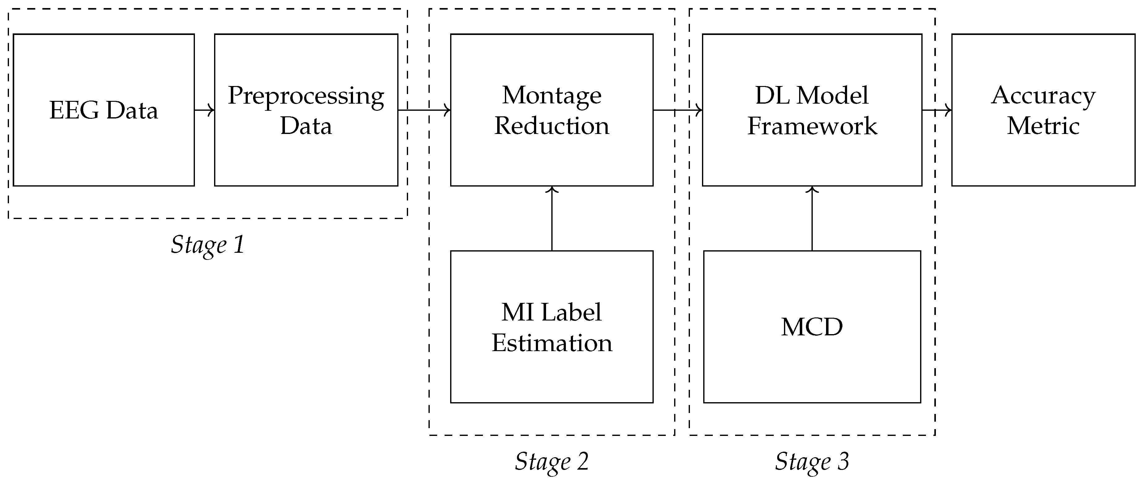
Figure 2.
Experimental timeline illustrating the structured sequence of events within a single MI trial conducted under the MI paradigm. The interval labeled as “Motor Imagery” represents the expected time window during which MI responses are elicited.
Figure 2.
Experimental timeline illustrating the structured sequence of events within a single MI trial conducted under the MI paradigm. The interval labeled as “Motor Imagery” represents the expected time window during which MI responses are elicited.
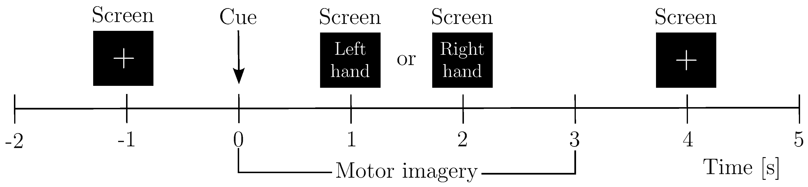
Figure 3.
Montage Reduction: Spatial arrangement of the four EEG electrode montages used in this study, based on the international 10–10 system: 8, 16, 32, and 64 channels.
Figure 3.
Montage Reduction: Spatial arrangement of the four EEG electrode montages used in this study, based on the international 10–10 system: 8, 16, 32, and 64 channels.
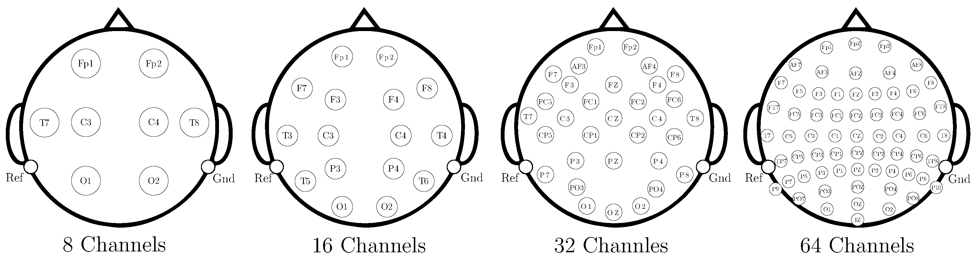
Figure 4.
Detailed architectures of the DL-based models evaluated for binary MI classification. All architectures employ a Softmax activation function after the final dense layer for label prediction. Nodes represent different layers, with arrows indicating their connections. Colors differentiate layer types, while outlines highlight specific layers within the same category.
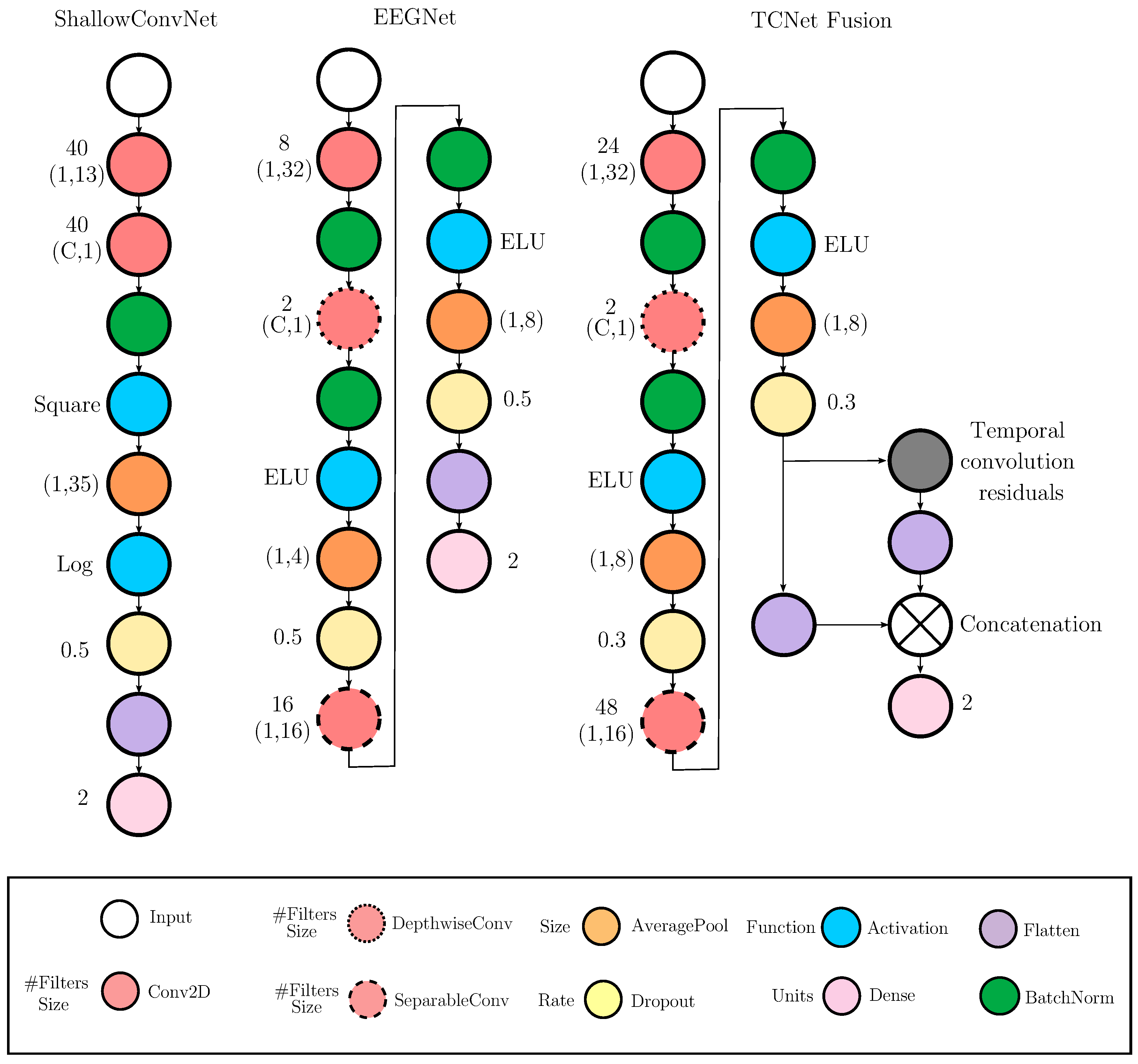
Figure 5.
Comparison of bi-class classification performance among state-of-the-art methods. Blue bars represent accuracy, orange bars denote Cohen’s Kappa, and green bars indicate the Area Under the Curve (AUC).
Figure 5.
Comparison of bi-class classification performance among state-of-the-art methods. Blue bars represent accuracy, orange bars denote Cohen’s Kappa, and green bars indicate the Area Under the Curve (AUC).
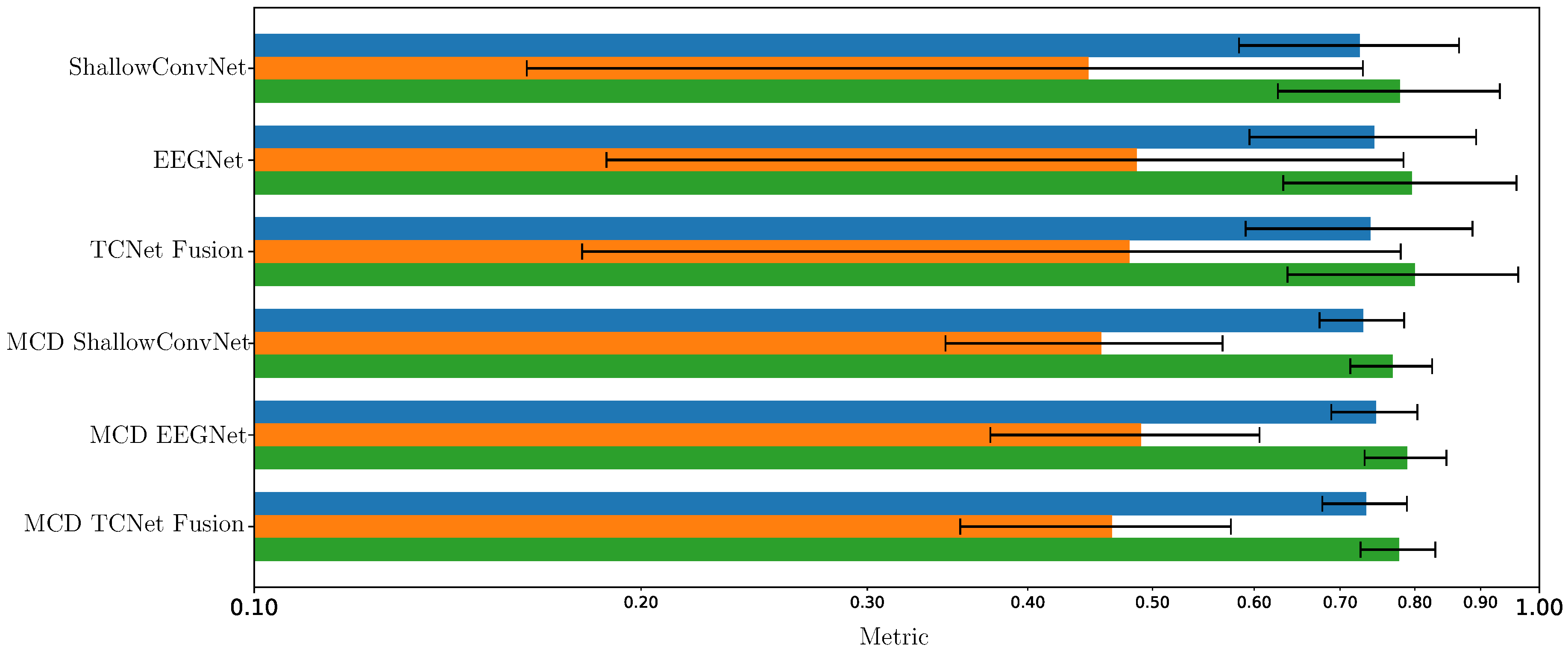
Figure 6.
Classification accuracy across channel configurations and models. The boxplots illustrate model-wise variability and robustness under different channel counts (8, 16, 32, and 64).
Figure 6.
Classification accuracy across channel configurations and models. The boxplots illustrate model-wise variability and robustness under different channel counts (8, 16, 32, and 64).
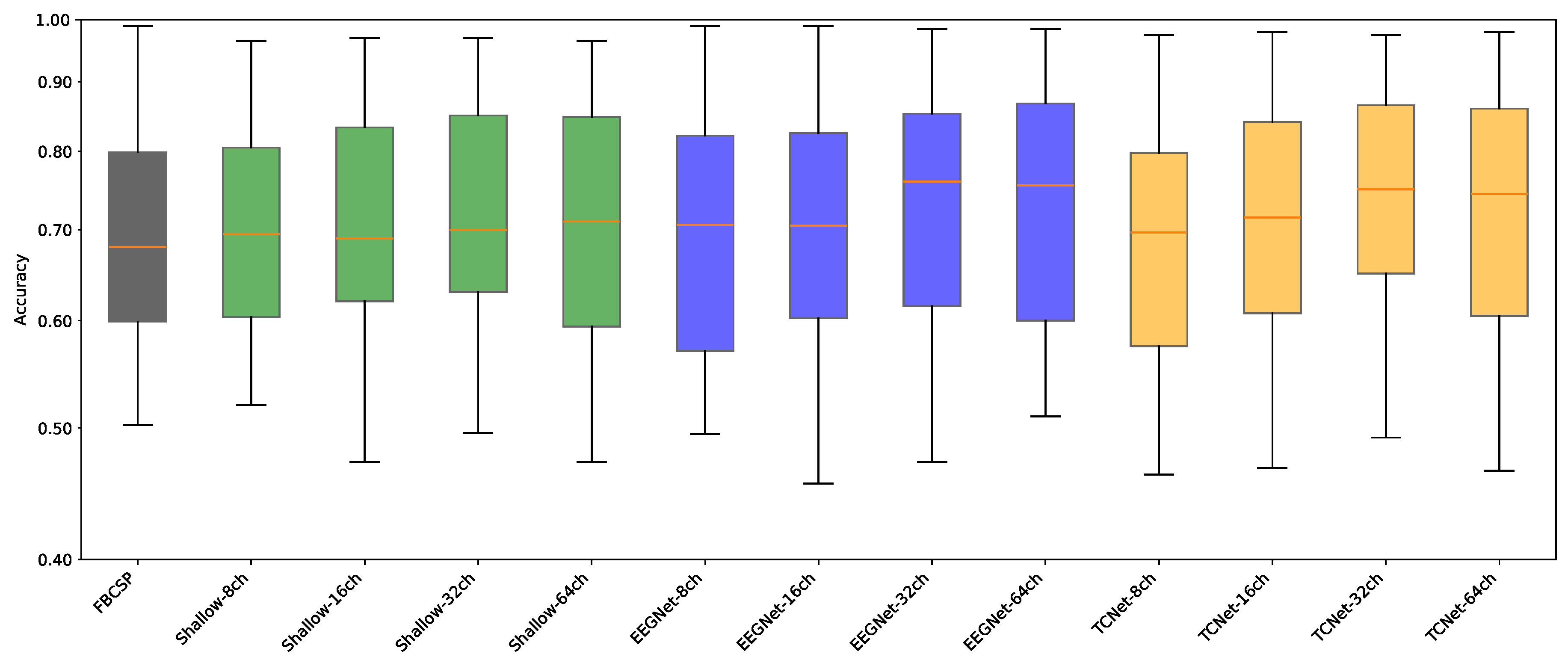
Figure 7.
Comparison of average classification accuracy across subjects for different models and channel montage configurations. In all three cases, each individual set is ranked according to the accuracy obtained using FBCSP (indicated by the black line). The dashed line plotted at the 70% accuracy level serves as a threshold for splitting individuals into best-performing (above this level) and worst-performing (below this level) groups. Note that the y-axis is on a log scale to improve the visibility of low accuracy values.
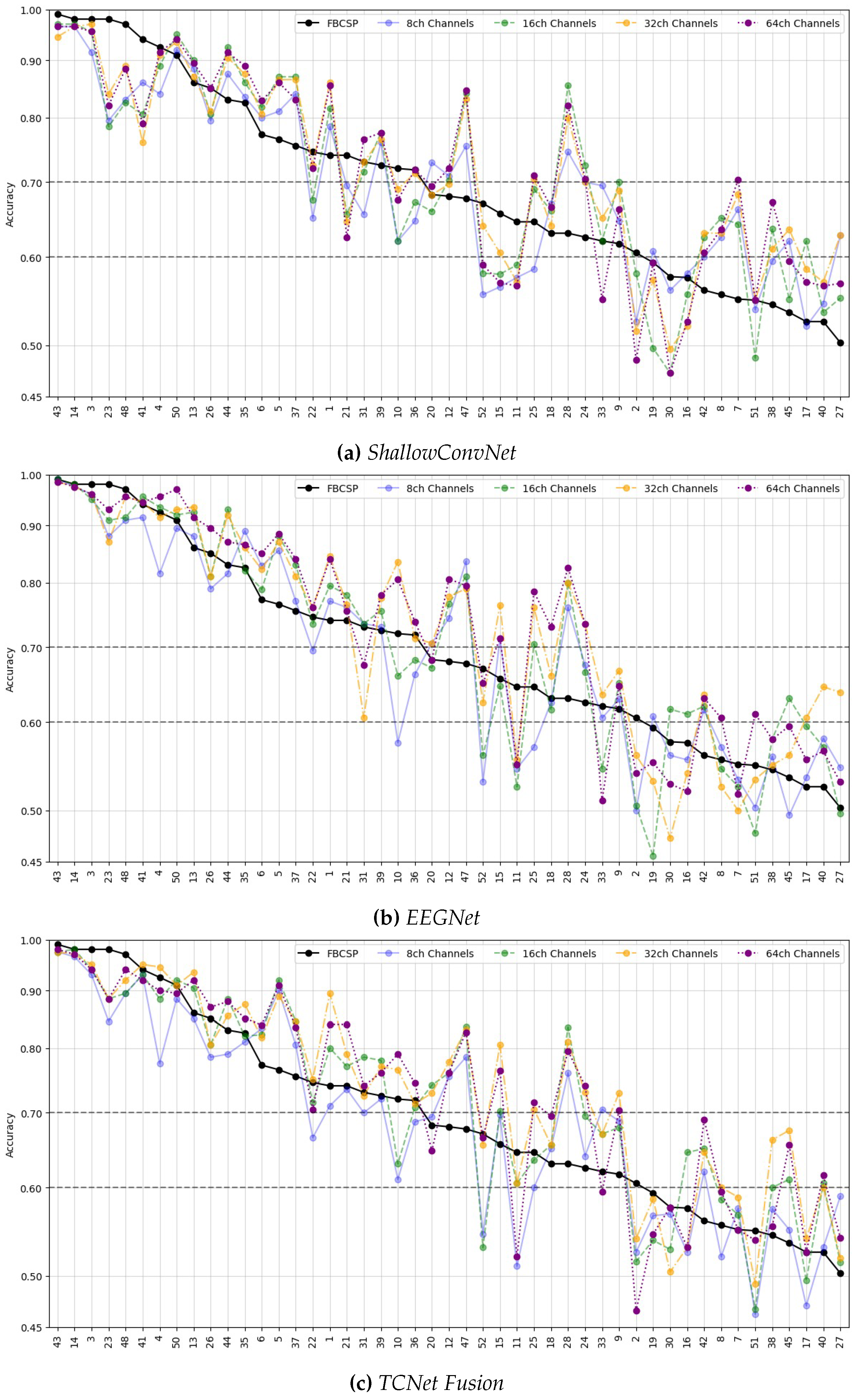
Figure 8.
Subject-wise analysis of EEG-based classification performance, highlighting the highest-performing model for each individual (denoted by an upward-pointing triangle) and the lowest-performing model (denoted by a downward-pointing triangle). Each deep learning model is color-coded to facilitate comparative interpretation.
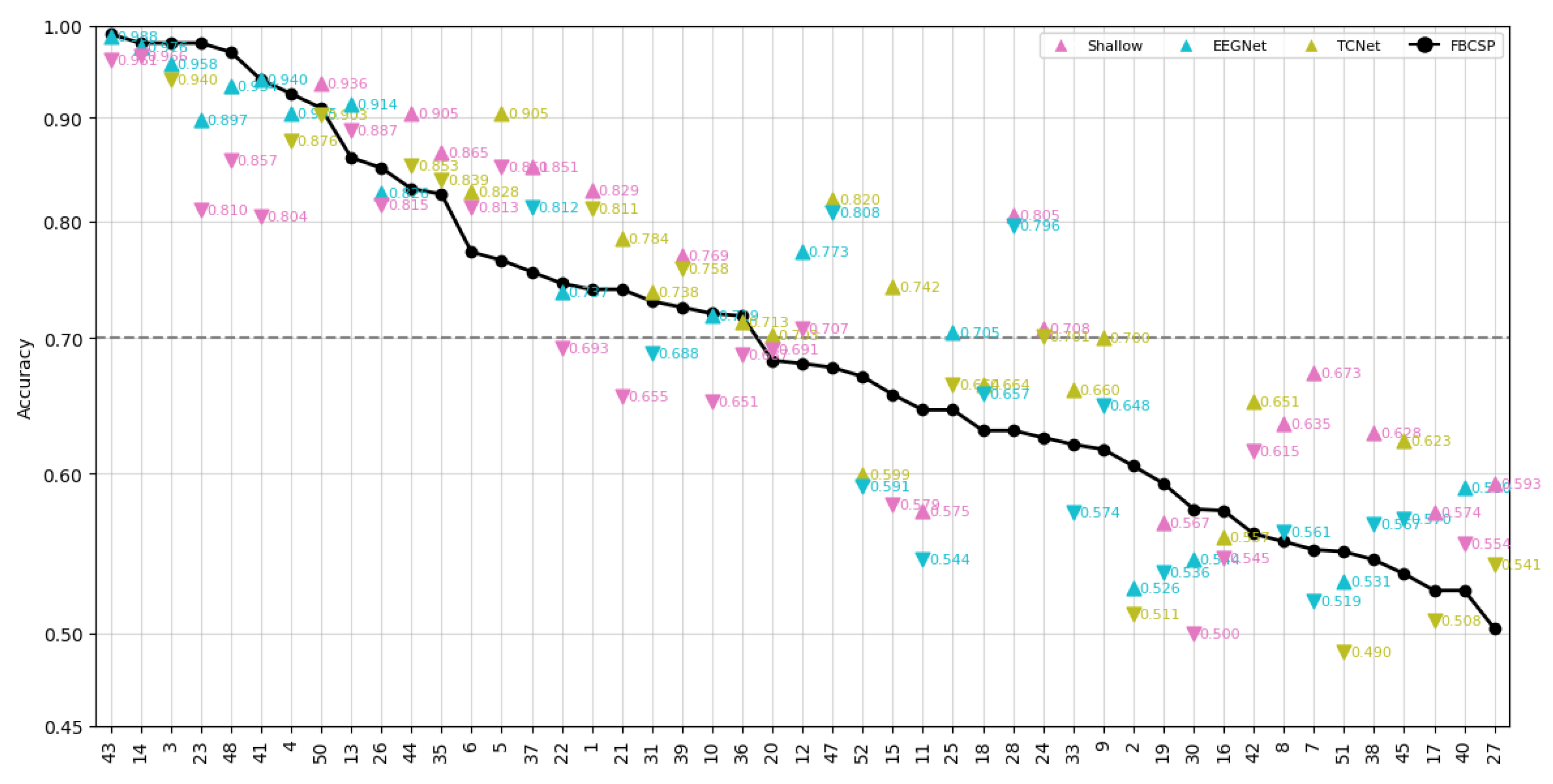
Figure 9.
Comparison of DL model performance (ShallowConvNet, EEGNet, TCNet Fusion) versus best classification accuracy across dropout rates in EEG-based motor imagery tasks, with the final row showing the optimal model and dropout rate per subject. A log scale is used on the y-axis to emphasize variability in low-accuracy subjects.
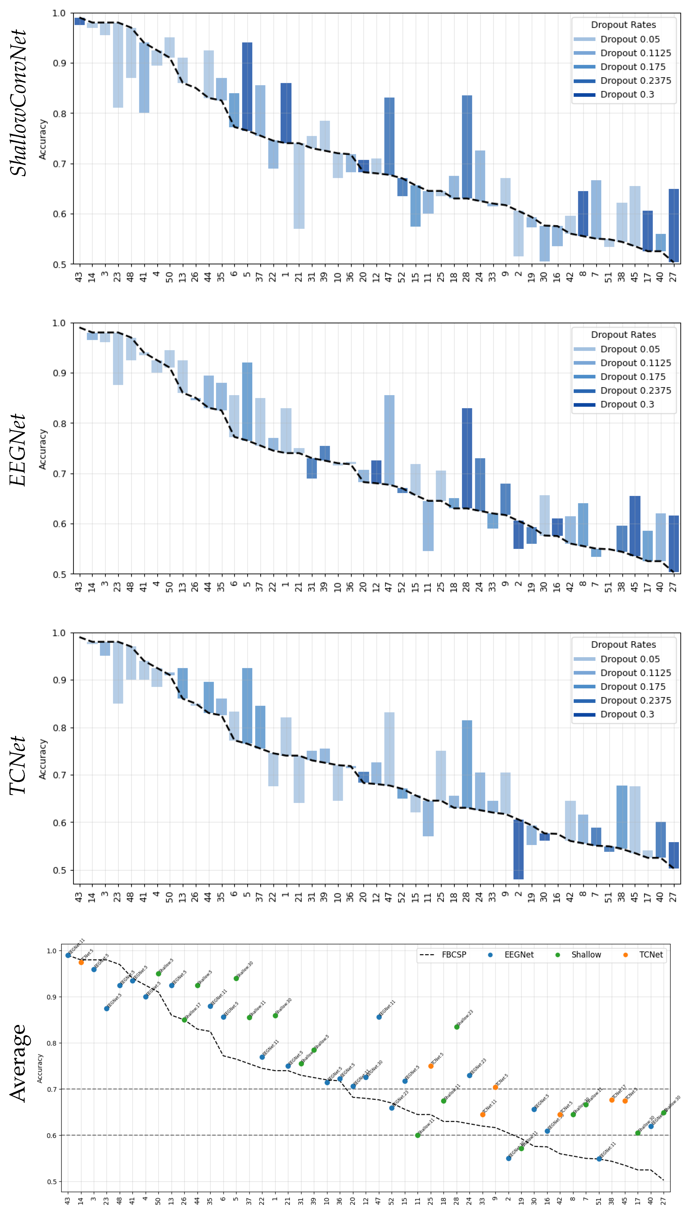
Figure 10.
Comparison of LayerCAM topographic activation maps between standard and MCD-enhanced models. Each subject is represented by a pair of maps: the left shows the standard model, and the right displays the MCD-enhanced version. The maps use a color scale in which yellow indicates high relevance, green denotes moderate relevance, and purple/dark blue – low relevance.
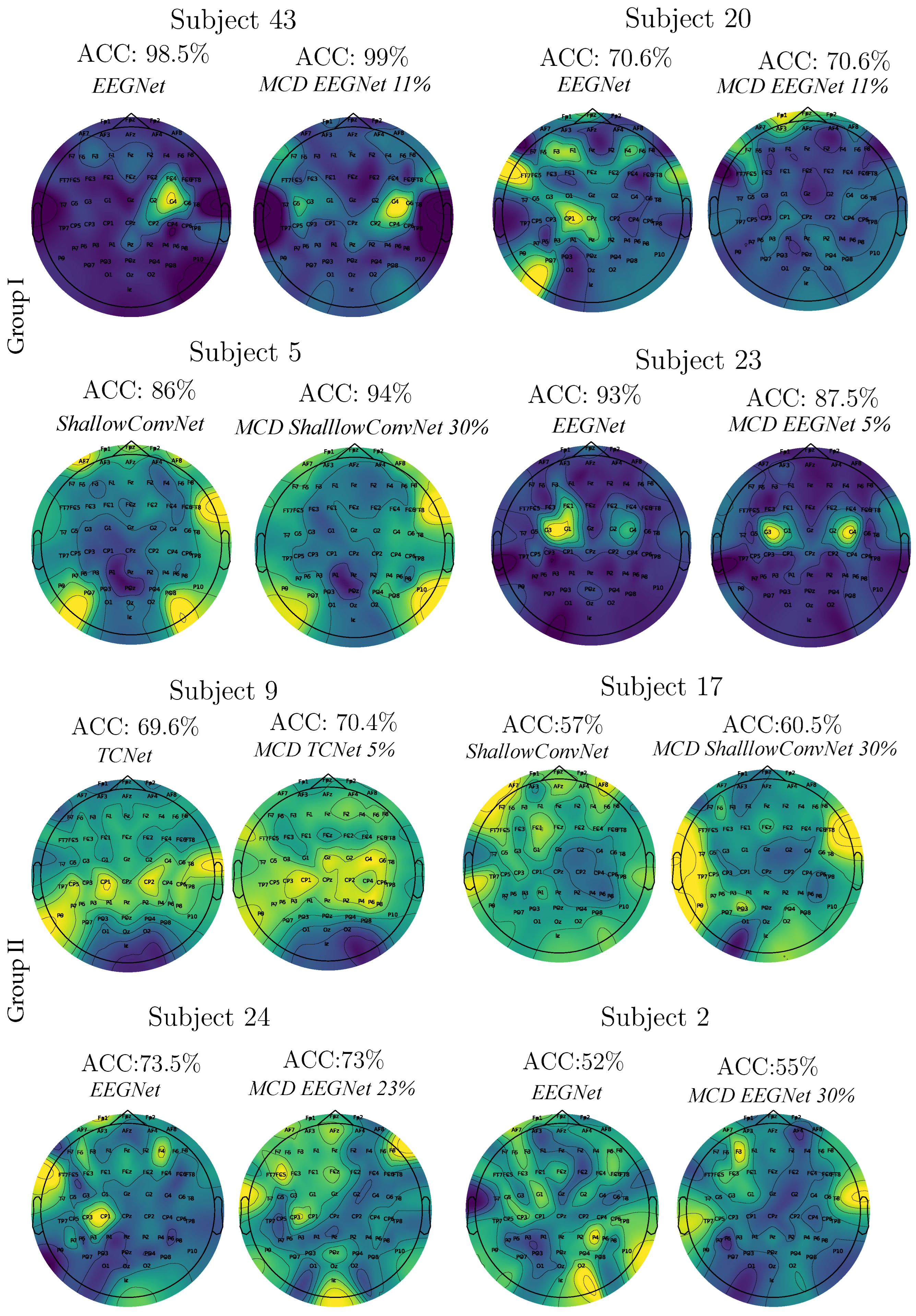

Table 1.
Performance consistency averaged across tested models and channel montages.
| Model | 8 Channels | 16 Channels | 32 Channels | 64 Channels |
|---|---|---|---|---|
| ShallowConvNet | ||||
| EEGNet | ||||
| TCNet Fusion |
Disclaimer/Publisher’s Note: The statements, opinions and data contained in all publications are solely those of the individual author(s) and contributor(s) and not of MDPI and/or the editor(s). MDPI and/or the editor(s) disclaim responsibility for any injury to people or property resulting from any ideas, methods, instructions or products referred to in the content. |
© 2025 by the authors. Licensee MDPI, Basel, Switzerland. This article is an open access article distributed under the terms and conditions of the Creative Commons Attribution (CC BY) license (http://creativecommons.org/licenses/by/4.0/).
Copyright: This open access article is published under a Creative Commons CC BY 4.0 license, which permit the free download, distribution, and reuse, provided that the author and preprint are cited in any reuse.


