
Submitted:
30 October 2025
Posted:
03 November 2025
You are already at the latest version
Abstract
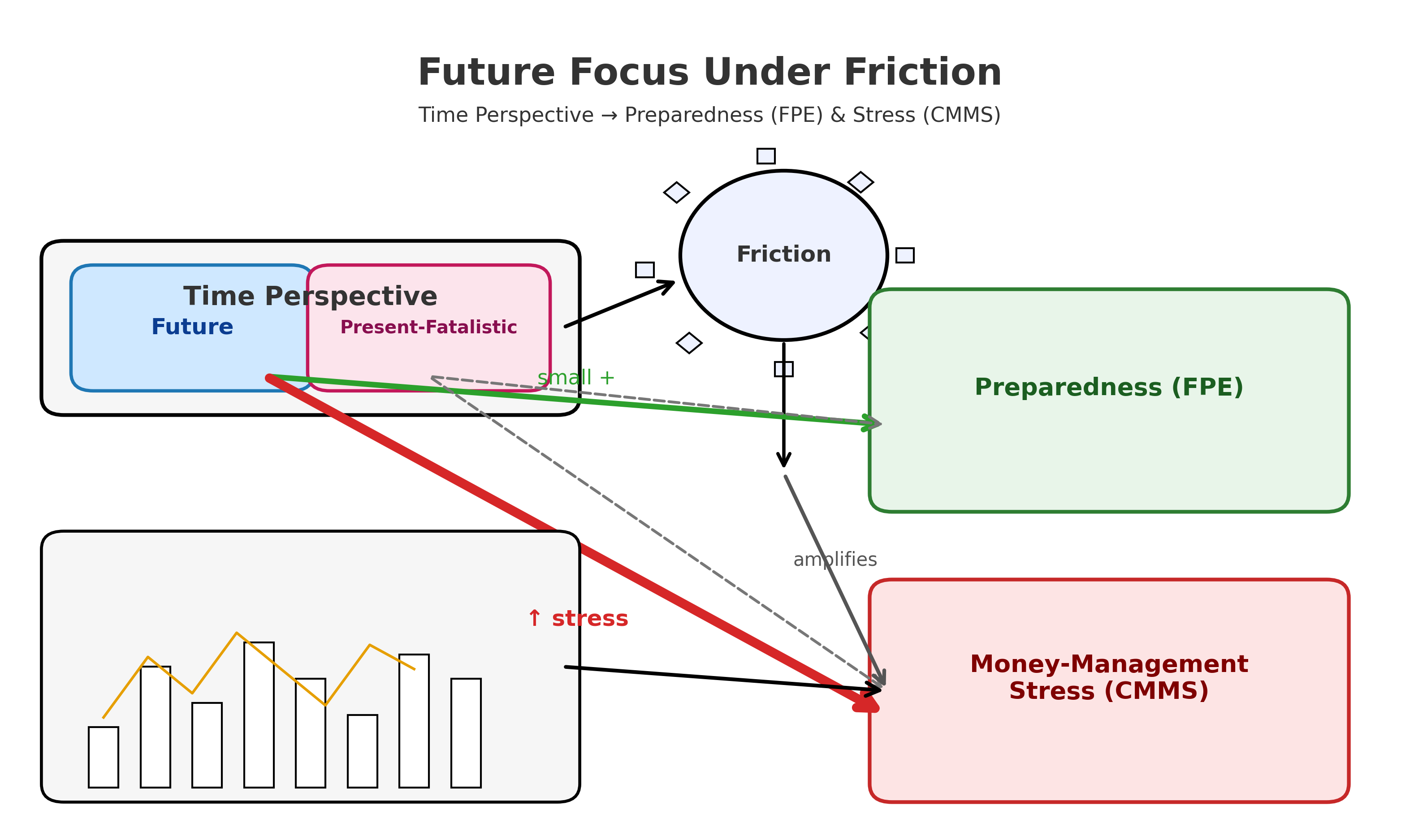
We tested whether two time-perspective dimensions–Future and Present-Fatalistic–explain financial functioning beyond income and demographics in a preregistered cross-sectional survey in Armenia (N=105; adult online sample; stratified convenience balancing sex, age bands, urban/rural). The constructs and predictions can be generalized to household finance. Outcomes were Financial Preparedness for Emergencies (FPE) and Current Money-Management Stress (CMMS). Preregistered hierarchical regressions with planned mediation tests showed that the time perspective added ~6 percentage points to FPE (ΔR²≈.06) and ~17 to CMMS (ΔR²≈.17). After multiple test adjustments, only the Future dimension remained clearly linked to higher CMMS scores, and Present-Fatalistic added nothing unique. Mediation via temporal orientation and buffering interactions were null. More future-focused participants reported greater day-to-day stress. We interpret Future→stress as higher standards and closer monitoring under everyday frictions and limited slack. The findings distinguish readiness from execution/strain and suggest pairing future self-interventions with friction-reducing tools.
Keywords:
time perspective
; financial preparedness
; money-management stress
; financial capability
; behavioral personal finance
1. Introduction
Households routinely face choices that require both near-term discipline and long-horizon preparation, such as budgeting this month while building buffers for shocks and retirement. Financial knowledge helps, but is rarely sufficient to produce robust financial capability. A growing body of work points to psychological time - how people habitually orient toward the future or the present - as a key ingredient shaping whether knowledge is translated into concrete behaviors such as planning, saving, and day-to-day money management (Lusardi & Mitchell, 2014; Zimbardo & Boyd, 1999). At the same time, structural resources (especially income) and demographics constrain what people can do and the bandwidth they bring to financial tasks (Mullainathan & Shafir, 2013).
This study focuses on two theoretically central time perspective dimensions, Future and Present-Fatalistic, and two complementary outcomes that capture “readiness” and “execution” in personal finance: FPE and CMMS, respectively. However, few studies jointly test these links while adjusting for socioeconomic status (SES) and demographics, leaving a clear gap this study addresses. We asked whether temporal orientations add explanatory power beyond income and demographics and whether they mediate or moderate the translation of resources into capabilities. Specifically, we test whether higher income is associated with lower present-fatalistic orientation (H1); whether present-fatalistic and future orientations are, respectively, negatively and positively related to FPE after controls (H2–H3); whether higher FPE predicts better money management (H4); whether income–capability links operate partly through temporal orientation (H5–H6); and whether future orientation buffers the adverse association between present-fatalistic and FPE (H8).
Methodologically, we preregistered a cross-sectional survey with validated measures (ZTPI Future and Present-Fatalistic; focused scales for FPE and CMMS with transparent scoring and reliability checks) and covariates (income, age, gender, residence). We then tested incremental validity (hierarchical regressions), mediation (including a chain path to CMMS), and a buffering interaction (Future × Present-Fatalistic) with multiple-comparison control and robustness diagnostics.
By concentrating on a parsimonious set of constructs and formally testing unique effects and mechanisms in a single framework, we clarify how psychological time helps convert resources into financial capability and where interventions might target temporal orientation (e.g., future focus) versus structural constraints (e.g., income).
Finally, while our data come from Armenia, the underlying mechanisms we test - intertemporal orientation operating under common household frictions - travel across settings. In Armenia, recent inflation, payment - timing frictions, and limited slack in household budgets make these mechanisms particularly salient. Under standard buffer-stock and consumption-smoothing logic, a stronger future focus should raise standards for precautionary balances and timely bill payments when slack is limited, whereas present-fatalistic beliefs should erode execution. Therefore, we expect the patterns we test to generalize to other settings with similar liquidity and institutional frictions.
2. Literature review
2.1. Financial Literacy and Capability
Financial literacy is a multidimensional construct encompassing knowledge, skills, experience, self-efficacy, and preparedness for shocks (Lusardi & Mitchell, 2014; Klapper, Lusardi, & van Oudheusden, 2015; OECD, 2020). Beyond its informational core, literacy functions as a behavioral resource that enables budgeting, saving, and contingency planning (Stolper and Walter, 2017). Early evidence has tied financial knowledge to concrete household practices such as bill payment, budgeting, and saving (Hilgert et al., 2003; Loibl & Hira, 2005). However, meta-analytic evidence shows that knowledge alone does not guarantee behavior change, highlighting the roles of motivation, self-beliefs, and context (Fernandes et al., 2014). Therefore, contemporary accounts treat financial literacy outcomes as the joint product of resources (e.g., income), cognitive orientations, and self-regulatory beliefs.
2.2. Temporal Orientation
A central cognitive orientation with direct implications for finances is the time perspective (TP). Zimbardo and Boyd’s (1999) framework distinguishes relatively stable tendencies to construe time as past-, present-, or future-oriented (with hedonistic and fatalistic facets of the present). A future orientation promotes planning, goal pursuit, and delay of gratification, all of which map onto emergency preparedness and systematic money management (Joireman, Sprott, & Spangenberg, 2005; Webley & Nyhus, 2006). Conversely, present-fatalistic orientations, marked by low perceived control and outcome expectancy, are theoretically antagonistic to long-horizon financial actions. Experimental and field evidence further suggest that strengthening psychological connections to one’s future self increases saving and retirement contributions (Hershfield et al., 2011), consistent with the idea that temporal focus shapes financial behavior.
Temporal orientation is also linked to perceived control and efficacy, two well-known psychological factors that affect self-regulation. Individuals who believe they have control over their lives and possess strong self-efficacy are more likely to establish financial objectives and adhere to them (Rotter, 1966; Bandura, 1997). Observational studies have associated internal control beliefs with increased savings and wealth creation, even when accounting for demographic factors (Cobb-Clarke et al., 2016). Additionally, socioeconomic gradients in perceived control are extensively documented: lower socioeconomic status (SES) correlates with a diminished sense of control throughout adulthood (Lachman & Weaver, 1998), educational trajectories influence control beliefs (Mirowsky & Ross, 2007), and SES affects the locus of control through cognitive and affective mechanisms (Gallo & Matthews, 2003). From this perspective, the time perspective may function both directly - by directing attention to future contingencies - and indirectly, by reinforcing the assumption that current actions might affect outcomes.
2.3. Socioeconomic Moderators & Control Beliefs
Socioeconomic resources shape psychological levers. Income is robustly associated with financial behaviors, but it also correlates with cognitive bandwidth, perceived control, and intertemporal trade-offs (Haushofer & Fehr, 2014; Mullainathan & Shafir, 2012; Mullainathan & Shafir, 2013). Scarcity can narrow the temporal focus toward the immediate present, increasing myopic decisions and reducing the capacity to engage in preventative actions. This suggests a plausible pathway whereby higher income is linked to less present-fatalistic and more future-oriented profiles, which in turn supports preparedness and better money management–an idea that positions temporal orientation as a mediator between income and financial functioning. Friction-reducing payment infrastructures (e.g., electronic and mobile payments) can also facilitate routine bill payments and budgeting and are increasingly being adopted across consumer segments (Greene & Stavins, 2021; Schuh & Stavins, 2012; Wang, 2024).
Gender differences remain salient in the financial domains. Men typically report higher confidence and engage more in investment activities, while women often score similarly or better on budgeting and day-to-day money management once access and experience are accounted for (Bucher-Koenen et al., 2017; Fonseca et al., 2012; Lusardi & Mitchell, 2014). Because gender is correlated with exposure to financial instruments and self-efficacy, controlling for demographics is essential when isolating the unique contribution of the time perspective to financial preparedness and management.
When considered collectively, previous research suggests an integrated process: structural resources (income) and demographics establish the context; temporal orientations (future versus present-fatalistic) influence individuals’ anticipation and planning for financial emergencies; and self-efficacy channels these orientations into effective FPE and CMMS. However, relatively few studies have jointly tested this sequence, asking whether temporal orientations explain incremental variance in FPE and CMMS beyond income and demographics and whether temporal orientations mediate or moderate links from socioeconomic factors to financial functioning.
Figure 1 summarizes the hypothesized relationships among resources, control beliefs, temporal orientation, and outcomes (FPE, CMMS).
Against this background, the present study asks to what extent future and present fatalistic orientations account for variation in FPE and CMMS after income and demographics are adjusted for and further probes the mechanisms: whether present fatalistic orientation mediates associations between income and financial functioning, whether future orientation buffers the adverse association between present fatalistic orientation and preparedness, and whether income’s association with money management is partly indirect through temporal orientation → FPE. By specifying these questions a priori and evaluating incremental, mediational, and interaction pathways in a single framework, we aim to clarify how psychological time helps translate resources into financial capabilities.
Taken together, these strands motivate our preregistered tests of incremental validity, mediation (including a chain path to CMMS), and a buffering interaction (Future×Present-Fatalistic) specified in the next section.
3. Research Questions and Hypotheses
Grounded in temporal perspective theory and research on financial self-regulation, this study investigates whether individual differences in time orientation account for the variance in financial functioning beyond socioeconomic characteristics. We focused on two dimensions of temporal orientation (future and present fatalistic) and examined their associations with two key outcomes: FPE and CMMS. Because income and demographics (age, gender, and residence) are established correlates of financial behavior, we treat them as covariates and ask whether temporal orientations provide incremental explanatory power over and above these factors. Accordingly, our primary research question is as follows: To what extent do future and present-fatalistic orientations explain the variance in FPE and CMMS after adjusting for income and demographics (RQ1)?
3.1. Numbering Aligns with the Preregistration:
H1–H4 are directional tests, and mediation, moderation, and chain questions are preregistered as RQs (RQ2–RQ4) without directional constraints.
3.2. Mapping.
RQ1 frames the incremental effects of temporal orientations on (a) FPE and (b) CMMS after controlling for covariates. The directional hypotheses H1–H4 address specific slopes within this framework (H1: Income→PF; H2–H3: PF/Future→FPE; H4: FPE→CMMS). RQ2 tests whether PF mediates the link between income and FPE/CMMS; RQ3 tests whether the future buffers the PF→FPE relationship; and RQ4 tests the chain path Income→Temporal Orientation→FPE→CMMS.
From a theoretical standpoint, future-oriented individuals are more likely to plan, delay gratification, and perceive themselves as capable of handling financial contingencies. Conversely, a fatalistic present orientation may erode perceived control and reduce engagement in preparatory behavior. These premises yield directional hypotheses that remain agnostic to their eventual magnitude and statistical significance. First, we hypothesized that income is negatively associated with Present-Fatalistic orientation (H1). Second, after controlling for income and demographics, Present-Fatalistic was negatively associated with FPE (H2), and Future was positively associated with FPE (H3). Third, higher FPE predicts better money management (lower CMMS), net of covariates (H4), and
Beyond these main effects, we tested preregistered process questions without directional constraints.
Why PF is a mediator (RQ2). Lower income can reduce perceived control and available bandwidth, fostering a more present-fatalistic mindset that suppresses preparedness and elevates day-to-day strain (Bandura, 1997; Mullainathan & Shafir, 2013; Rotter, 1966). Why Future as a moderator (RQ3). A stronger future orientation supports goal maintenance, delay of gratification, and plan enactment, thereby attenuating PF’s negative association between PF and preparedness (Zimbardo & Boyd, 1999).
RQ2 (mediation, preregistered). Does Present-Fatalistic mediate the links between income and FPE and CMMS? RQ3 (Moderation, preregistered). Does the Future buffer the adverse association between Present-Fatalistic and FPE (i.e., Future×PF → FPE is positive for preparedness)? RQ4 (chain mediation, preregistered). Is the association between income and CMMS partly indirect via temporal orientation → FPE (Income → Temporal Orientation → FPE → CMMS)?
Analytically, we estimated hierarchical models with income and demographics entered first, followed by temporal orientations (addresses RQ1 / H2–H3 for FPE and RQ1 for CMMS). Mediation and chain paths (RQ2, RQ4) used bias-corrected bootstrap CIs for indirect effects, and moderation (RQ3) used the Future×PF interaction with mean-centered predictors. We will verify the coding direction for all scales (reversing where necessary to maintain a consistent interpretation), report standardized coefficients with 95% confidence intervals, and apply false-discovery-rate control within families of related tests. Robustness checks include alternative codings of income (ordinal vs. continuous), heteroskedasticity-consistent standard errors, and influence diagnostics. This design allows us to adjudicate whether temporal orientations meaningfully contribute to financial preparedness and money management above socioeconomic factors while remaining fully neutral about the eventual pattern of results.
Together, these tests adjudicate whether temporal orientations contribute to preparedness and money management above socioeconomic factors and how (incremental, mediated, buffered, and chained pathways).
4. Methods
4.1. Design and Preregistration
We used a cross-sectional survey design to test directional hypotheses about temporal orientation, FPE, and CMMS, while controlling for income and demographics. The study specified the analysis plan (outcomes, covariates, model blocks, mediation/moderation tests, and robustness checks) a priori. Materials, code, and de-identified data are available in an open repository.
4.2. Participants and Sampling
Participants were adults (18+) recruited via university mailing lists and community social media in Armenia using stratified quota-based convenience sampling (non-probability) to balance sex, age bands (18–29, 30–44, 45–60), and region (urban/rural). We used quotas to approximate the distribution of sex, broad age bands, and urban/rural residence; however, the design was non-probabilistic, and online self-selection may have biased the sample toward more digitally engaged respondents. The inclusion criteria were residence in Armenia and the ability to complete the survey in Armenian or English. The exclusion criteria were straight-lining on >50% of the items, completion time of less than one-third of the median, or failing two attention checks. An a priori power analysis for hierarchical multiple regression (Block 1: four covariates; Block 2: two focal predictors) indicated that detecting a small-to-moderate incremental effect (ΔR²≈.06–.08; Cohen’s f²≈.06–.09) at α=.05 and 1–β=.80 required a sample size of approximately N≈110–150. Final analysis: N=105 after exclusions (target N≈120–150).
4.2.1. Power and Sample Size
Our preregistration targeted N=110–150 for hierarchical models with covariates entered first and temporal orientations added in Block 2. The final sample analyzed was N=105 after pre-registered exclusions (e.g., incomplete responses and failed attention checks). A sensitivity check indicated that, at α=.05, this sample afforded adequate power to detect small-to-moderate incremental effects in Block 2, whereas mediation and moderation effects typically require larger samples; accordingly, these process tests should be interpreted cautiously.
4.2.2. Data Screening and Outliers
Following preregistration, we inspected continuous variables for extreme values and winsorized them at the prespecified tails to reduce undue influence (i.e., capped extremes rather than removed cases). Winsorization does not change N; the difference between the target range and our final N reflects the preregistered exclusions (missingness/attention). The results were robust to alternative cutoffs and models estimated without winsorization (see Supplement).
4.3. Procedure and Ethics
After providing informed consent, the participants completed an online survey. This study was conducted in accordance with the Declaration of Helsinki and received Institutional Review Board approval. No deception was used. Participants could skip any question and withdraw from the study at any time.
4.4. Measures
4.4.1. Time Perspective
Time perspective was measured using the Zimbardo Time Perspective Inventory (ZTPI), using the Future and Present-Fatalistic (PF) subscales as focal predictors from the original 56-item ZTPI (used for all participants). The items were rated on a 5-point frequency scale. For each subscale, we computed the mean score (higher = more of the construct). For the Armenian version, we used translation - back-translation, expert reconciliation, and pilot testing (n≈20) to assess item clarity. Reliability: Future: α (polychoric) = .78, ω (total) = .80; Present-Fatalistic: α (polychoric) = .72, ω (total) = .74. .
4.4.2. Financial Outcomes
Financial preparedness for emergencies (FPE). FPE was assessed using the Financial Preparedness for Emergency subscale adopted from the publisher-provided research instrument reported by Lone and Bhat (2024). Items were rated on a Likert-type response format and combined into a composite by z-standardizing and averaging the item scores (higher values = greater preparedness/efficacy). Internal consistency: α (polychoric) = .84, ω (total) = .86; one-factor CFA (Comparative Fit Index, CFI; Tucker–Lewis Index, TLI; Root Mean Square Error of Approximation, RMSEA; Standardized Root Mean Square Residual, SRMR).
Current Money-Management Stress (CMMS). Day-to-day money-management stress was measured using the CMMS subscale of the Perceived Financial Well-Being (PFWB) scale, with items adopted from the same publisher-provided instrument in Lone and Bhat (2024). The items were keyed so that higher values indicated greater stress. CMMS indexes perceived money-management stress (e.g., pressure, worry, and strain). Higher CMMS scores indicate more stress; they do not necessarily imply poorer day-to-day management performance. Internal consistency: α (polychoric) = .88, ω (total) = .90; CFA indices (CFI, TLI, RMSEA, and SRMR). As a descriptive robustness examination, we additionally computed a brief behavior index (budgeting, expense tracking, on-time bill payment, automated saving), which was used only for secondary analysis.
Note. Constructs such as “financial awareness,” “experience,” and “skills” were reserved for secondary analyses; any bespoke items were kept separate from the primary FPE/CMMS outcomes to avoid construct drift.
4.4.3. Income and Demographics (Covariates)
Participants reported monthly household income in ordered categories (converted to midpoints for sensitivity analyses), age (years), sex (male/female/other), and region (urban/rural). Income and demographics entered Block 1 of the hierarchical models.
4.4.4. Reasoning/Numeracy (Control; Optional Robustness)
Instead of an undefined “rationality test,” we included brief, validated indices: the Cognitive Reflection Test (CRT-2/CRT-Long short) and Berlin Numeracy Test (adaptive). Scores were adjusted to a common scale and could be used as additional factors to check if time-related effects continued, regardless of reasoning or numeracy
4.5. Data Quality and Preprocessing
We preregistered the attention checks, long-string detection, and response time flags. Missing item responses <10% within a scale were imputed by person-mean if scale α≥.70; otherwise, cases were listwise deleted for that analysis. At the dataset level, if missingness exceeded 5%, we used Multivariate Imputation by Chained Equations (MICE) for the sensitivity analyses. Continuous predictors were z-standardized, and interactions used mean-centered components. We screened for outliers (|z|>3.5), influential points (Cook’s D), and multicollinearity (Variance Inflation Factor (VIF)<5).
4.6. Statistical Analysis and Modeling Plan
4.6.1. Outcomes
We analyzed two outcomes separately: (1) FPE and (2) CMMS. For all models, we report standardized coefficients (β), HC3 heteroskedasticity-robust standard errors (SEs), 95% confidence intervals (CIs), and ΔR² where applicable.
4.6.2. Predictors and Covariates
The focal predictors were the ZTPI Future and Present-Fatalistic (PF) subscales. Covariates included income, age, gender (male = 1), and residence entered as two dummies with the capital city as the reference category (other city = 1/0; village = 1/0). Continuous predictors were mean-centered and standardized prior to the analysis.
4.6.3. Primary Analyses (Incremental Validity)
We estimated hierarchical linear regressions to test whether temporal orientations added explanatory power beyond demographics and income.
- Block 1 (covariates): Income, Age, Gender, Residence dummies.
- Block 2 (focal predictors): Future, PF.
For each outcome (FPE; CMMS), we report ΔR² from Block 1 → Block 2, along with standardized βs, HC3 SEs, and 95% CIs.
4.6.4. Mediation Tests
Using bias-corrected bootstrap (2,000 resamples), we estimated the indirect effects for (a) Income → PF/Future → FPE and (b) the chain Income → PF/Future → FPE → CMMS. Indirect effects were considered different from zero when the 95% CI excluded zero.
4.6.5. Moderation Test (Buffering)
To examine whether a future time perspective attenuated PF’s negative association between PF and FPE, we added the Future × PF interaction to the FPE model. Simple slope tests were probed at ±1 standard deviation (SD) after standardization/mean centering.
4.6.6. Multiple Comparisons.
Within each outcome family, we controlled the false discovery rate using Benjamini–Hochberg at q = .05.
4.6.7. Diagnostics and Robustness of the Model.
We examined linearity, residual distribution and homoscedasticity, collinearity (VIF < 5), leverage, and Cook’s D. If violations continue, we re-estimate the key models using a robust regression MM estimator. Robustness checks include: (i) alternative income specifications (ordinal categories vs. continuous midpoints), (ii) winsorizing income at 1%, and (iii) optionally adding reasoning/numeracy controls (CRT, numeracy) to assess the stability of the focal effects.
4.6.8. Equivalence Testing (Urban/Rural).
When group sizes were adequate, we assessed Two One-Sided Tests (TOST) equivalence on FPE and CMMS for urban/rural contrasts using the Smallest Effect Size of Interest (SESOI) |d| ≤ 0.33.
4.6.9. Reporting and Transparency.
We provide a comprehensive measurement table (constructs, items, scales, scoring direction, α/ω, reverse-coded items), full correlation matrices with 95% CIs, and descriptive statistics (M, SD, range) for all the variables. The data, syntax, and analysis outputs will be archived in an open repository.
4.6.10. Compact Model Specifications.
Here, res_other and res_village denote the residence dummy variables (capital = 0).
FPE model (with moderation):
FPE = β₀ + β₁·Income + β₂·Age + β₃·Gender + β₄·res_other + β₅·res_village + β₆·Future + β₇·PF + β₈·(Future×PF) + ε.
CMMS model:
CMMS = β₀ + β₁·Income + β₂·Age + β₃·Gender + β₄·res_other + β₅·res_village + β₆·Future + β₇·PF + ε.
Indirect paths: Income → {PF, Future} → FPE → CMMS.
4.6.11. Rationale
This plan tests (i) the incremental validity of temporal orientations beyond socioeconomic and demographic factors, (ii) whether temporal orientations mediate the translation of resources (income) into financial preparedness and downstream money management, and (iii) whether future orientation buffers the adverse association between PF and FPE.
5. Results
5.1. From Correlations to Multivariable Tests.
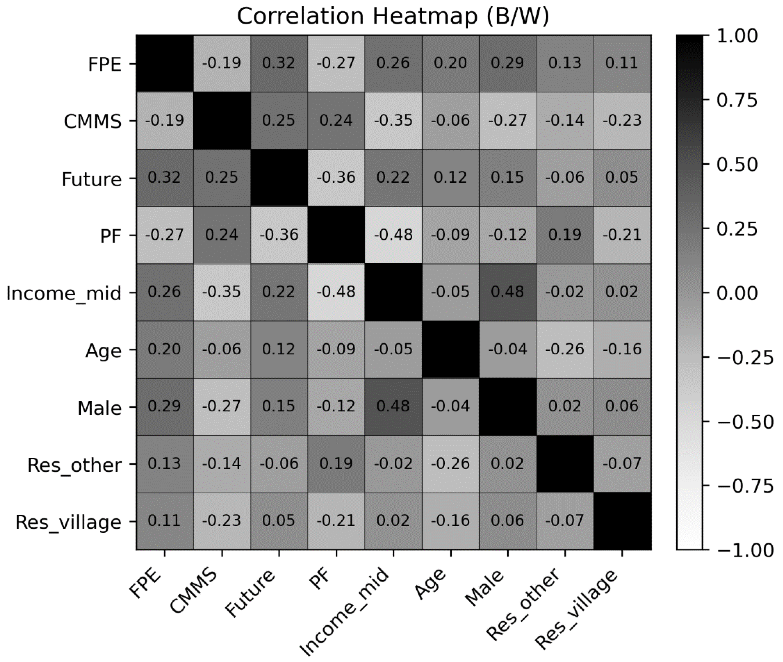
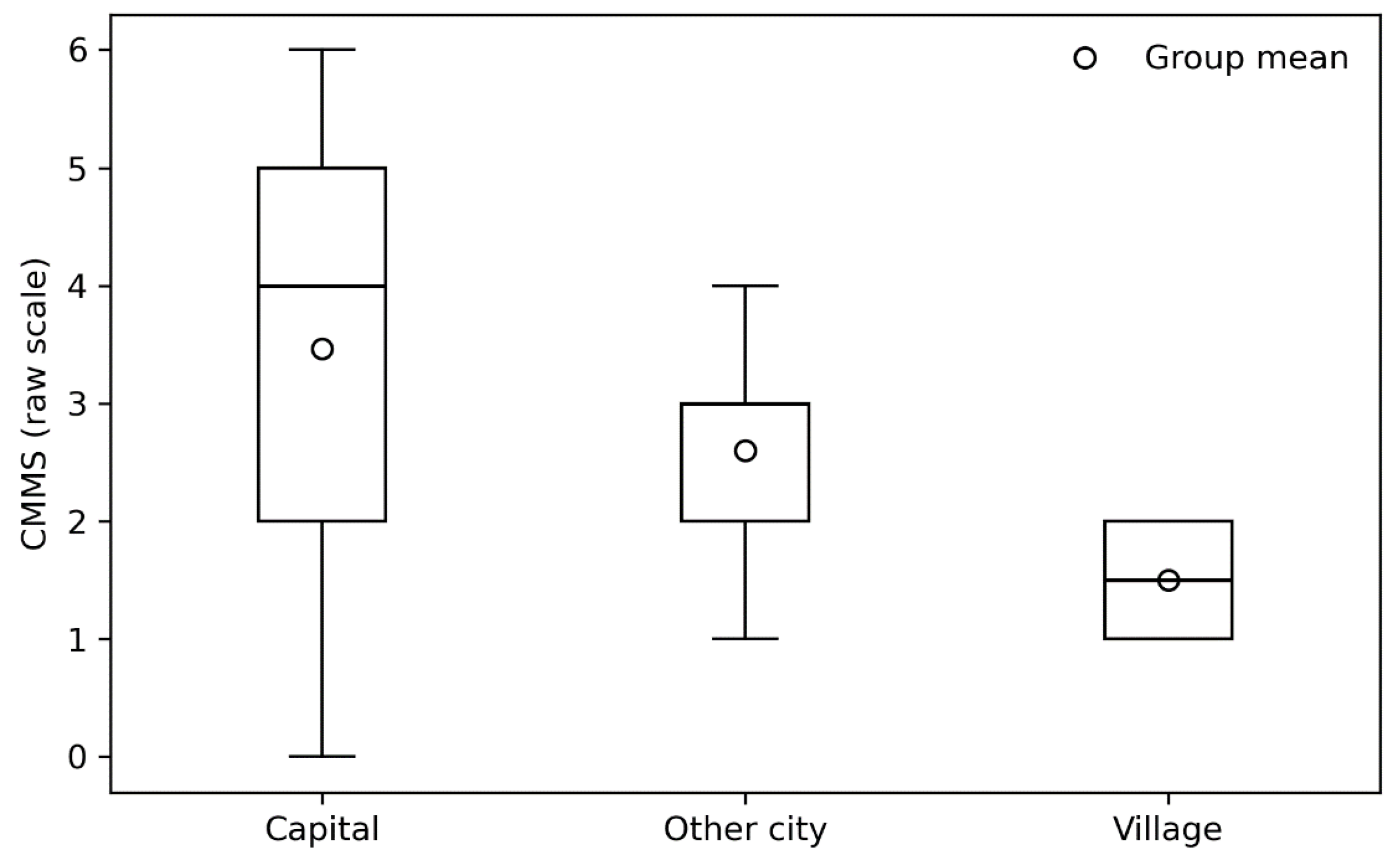
The zero-order correlations suggest three substantive patterns: (i) higher income ↔ (is associated with) lower Present-Fatalistic (PF) (r = −.448, p = .001); (ii) Future orientation ↔ higher FPE (r = .290, p = .037) and PF ↔ lower FPE (r = −.326, p = .018); and (iii) higher income ↔ better current money management (CMMS; r = −.365, p = .008; higher scores indicate more stress). A gender difference in FPE was observed (M_male = 2.79 vs. M_female = 2.03; p = .027), whereas urban/rural comparisons were not significant. Correlations between a brief “rationality” index and financial outcomes were uniformly non-significant.
Because bivariate associations do not adjust for confounding or overlap among predictors and because the income–time-perspective–FPE/CMMS links may be partly indirect, we proceeded with hierarchical and path-analytic models.
Block 1 and 2 effects and multiple testing summary. Adding Future and Present-Fatalistic produced a modest gain in explained variance for preparedness (FPE; ΔR² ≈ .06) and a meaningful gain for money-management stress (CMMS; ΔR² ≈ .17). Nominal tests indicated several focal slopes, but after false discovery rate (FDR) correction, only the positive Future → CMMS association remained robust; other focal effects should be viewed as exploratory. For clarity, we report standardized coefficients with 95% HC3 confidence intervals and FDR-adjusted p-values; complete technical details and additional diagnostics are provided in the Supplement.
5.2 Hierarchical Regressions
Block 1 included income, age, gender (male = 1), and residence (two dummies with capital as a reference: other cities and villages). Block 2 added future and present fatalistic (PF) time-perspective predictors. All coefficients are standardized; SEs are HC3; 95% CIs were reported.
5.2.1. Financial Preparedness for Emergencies (FPE)
Adding Future and PF yielded a modest but meaningful increment in the explained variance (R² = .205 → .268; ΔR² = .064, a modest gain in explained variance).

Table 1.
Hierarchical model and incremental validity for FPE (standardized coefficients, 95% HC3 CIs, and FDR-adjusted p-values).
Table 1.
Hierarchical model and incremental validity for FPE (standardized coefficients, 95% HC3 CIs, and FDR-adjusted p-values).
| Predictor | Block 1 β [95% CI] | p | Block 2 β [95% CI] | p |
| Income (midpoint) | 0.175 [0.008, 0.342] | 0.039 | 0.055 [−0.163, 0.274] | 0.620 |
| Age | 0.292 [0.100, 0.483] | 0.003 | 0.247 [0.039, 0.456] | 0.020 |
| Sex | 0.203 [0.042, 0.364] | 0.013 | 0.213 [0.042, 0.383] | 0.014 |
| Residence - other city (vs. capital) | 0.210 [0.132, 0.289] | < .001 | 0.234 [0.159, 0.308] | < .001 |
| Residence - village (vs. capital) | 0.155 [0.037, 0.273] | 0.010 | 0.112 [0.000, 0.223] | 0.050 |
| Future | - | - | 0.197 [0.002, 0.391] | 0.047 |
| Present-Fatalistic (PF) | - | - | −0.148 [−0.346, 0.050] | 0.144 |
Model fit: R² (Block 1) = 0.205; R² (Block 2) = 0.268; ΔR² = 0.064 (a modest gain in the explained variance).
Notes. N = 105. All coefficients were standardized, the and CIs were HC3-based. p values are two-sided. Sex coding and income midpoint construction followed the Methods. The full specification table (unstandardized B, HC3 SEs, raw p, VIF, and diagnostics) is presented in Table S4 (Supplement).
Block 1:
- Future: β = .197, 95% CI [.002, .391], p = .047 (FDR-adjusted p = .094).
- PF: β = −.148, 95% CI [−.346, .050], p = .144 (ns).
- Age: β = .247, 95% CI [.039, .456], p = .020.
- Male: β = .213, 95% CI [.042, .383], p = .014.
- Residence - Other city (vs. capital): β = .234, 95% CI [.159, .308], p < 10⁻⁹.
- Residence - Village (vs. capital): β = .111, 95% CI [.000, .223], p = .050.
- Income (midpoints): β = .055, p = .620 (ns).
Interpretation. Controlling for covariates, future orientation was positively associated with FPE (nominal p < .05, not surviving FDR). PF showed no unique association. Older age, being male, and living outside the capital predicted higher FPE.
5.2.2. Current Money-Management Stress (CMMS; Higher = More Stress)
Adding Future and PF produced a substantial increase in the explained variance (R²: .232 → .400; ΔR² = .168, a meaningful gain in the explained variance).
Table 2.
Hierarchical model and incremental validity for CMMS (standardized coefficients, 95% HC3 CIs, adjusted p).
Table 2.
Hierarchical model and incremental validity for CMMS (standardized coefficients, 95% HC3 CIs, adjusted p).
| Predictor | Block 1 β [95% CI] | p | Block 2 β [95% CI] | p |
| Income (midpoint) | −0.299 [−0.513, −0.084] | 0.006 | −0.266 [−0.504, −0.027] | 0.029 |
| Age | −0.169 [−0.311, −0.028] | 0.019 | −0.207 [−0.364, −0.051] | 0.010 |
| Sex | −0.115 [−0.344, 0.115] | 0.329 | −0.173 [−0.379, 0.034] | 0.101 |
| Residence - other city (vs. capital) | −0.207 [−0.352, −0.062] | 0.005 | −0.230 [−0.393, −0.067] | 0.006 |
| Residence - village (vs. capital) | −0.253 [−0.475, −0.032] | 0.025 | −0.233 [−0.400, −0.067] | 0.006 |
| Future | - | - | 0.440 [0.258, 0.621] | < .001 |
| Present-Fatalistic (PF) | - | - | 0.223 [−0.020, 0.466] | 0.072 |
Model fit: R² (Block 1) = 0.232; R² (Block 2) = 0.400; ΔR² = 0.168 (a meaningful gain in the explained variance).
Notes. N = 105. CMMS is coded such that higher scores indicate more stress (positive β = higher stress). Coefficients are standardized; CIs are HC3-based; two-sided p-values reported. Full specifications (unstandardized B, HC3 SEs, raw p, VIF, diagnostics) are presented in Table S5 (Supplement).
Block 2
- Future : β = +.440, 95% CI [+.258, +.621], p = 0.000002 (survives FDR, q < .01).
- PF: β = + .223, 95% CI [−.020, +.466], p = .072 (trend).
- Income: β = −.266, 95% CI [−.504, −.027], p = .029.
- Age: β = −.207, 95% CI [−.364, −.051], p = .010.
- Male : β = −.173, p = .101 (ns).
- Residence - Other city (vs capital): β = −.230, 95% CI [−.393, −.067], p = .0056.
- Residence - Village (vs capital): β = −.233, 95% CI [−.400, −.067], p = .0060.
Figure 2 shows a side-by-side forest plot of the standardized Block-2 coefficients (HC3 95% CIs) for both outcomes.
Interpretation. The dominant, FDR-robust result was that higher future orientation predicted more money-management stress after adjustment. PF showed a positive trend with stress. In contrast, higher income and older age predicted less stress, and residents outside the capital reported lower stress than those in the capital.
5.3. Multiple-Comparison Control
The Benjamini–Hochberg FDR (q = .05) analysis of the four focal slopes, which included Future and PF in both FPE and CMMS, indicated that only the Future → CMMS slope remained significant after correction (raw p = 2×10⁻⁶; FDR p = 8×10⁻⁶). The Future → FPE slope was nominally significant (p = .047), but did not survive the FDR (q ≈ .094). The marginal effect of Future on CMMS is illustrated in Figure 3.
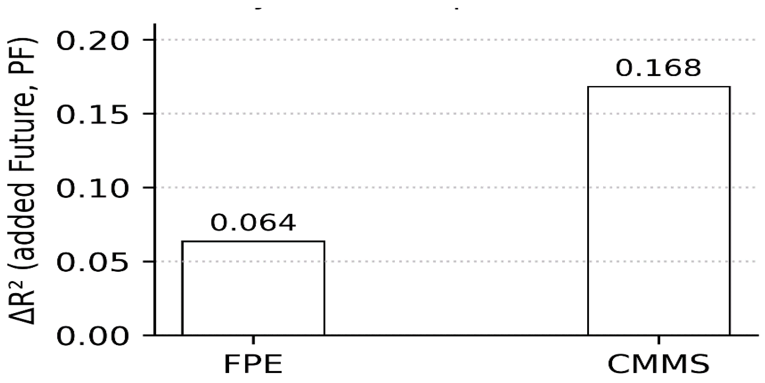
The incremental variance explained by adding time perspective variables is summarized in Figure 4 (ΔR²_FPE = .064; ΔR²_CMMS = .168).
5.4. Mediation and Chain Mediation
Bias-corrected bootstrap (2,000 resamples) showed no significant indirect effects (all 95% CIs include zero):
- Income → PF → FPE: point = .080, 95% CI [−.029, .217].
- Income → Future → FPE: point = .040, 95% CI [−.004, .107].
- Income → PF → FPE → CMMS (chain): point = −.006 (sign flipped), 95% CI [−.026, +.013].
- Income → Future → FPE → CMMS (chain): point = −.003 (sign flipped), 95% CI [−.013, +.004].
Therefore, temporal orientations did not influence the relationship between income and FPE/CMMS, and we did not observe a link between FPE and CMMS.
5.5. Moderation (Buffering).
The Future × PF interaction predicting FPE was not significant (β = .024, p = .827). The simple slopes of Future at PF ±1 SD were also non-significant (β = .176, p = .153; β = .223, p = .202). There is no evidence that future orientation buffers PF’s adverse link to preparedness.
5.6. Diagnostics and Robustness.
Collinearity was low (all the VIFs ≤ 1.75). The results were stable when ordinal income was used instead of midpoints and when income was winsorized at 1%. Urban/rural TOST equivalence tests were not run because of severe imbalance (urban, n = 100; rural, n = 4).
After adjustment, future orientation was positively associated with money-management stress and positively associated with preparedness (FPE) at the nominal level; the former was the only focal effect that remained significant after FDR correction.
6. Discussion
After adjusting for income and demographics, Future was positively associated with CMMS and showed a nominal positive association with FPE that did not survive FDR correction. PF showed no unique associations after the correction. Adding time perspectives yielded a modest increment for the FPE (ΔR² ≈ .06) and a meaningful increment for the CMMS (ΔR² ≈ .17). Mediation from income through temporal orientation and the preregistered Future × PF buffering test was null. Taken together, temporal orientations added limited explanatory power for preparedness and concentrated associations on stress, whereas income and age showed direct stress-reducing associations, and stress was lower outside the capital.
6.1. Interpreting the Future - Stress Effect: A Vigilance–Friction Account.
Why might a stronger future focus be associated with higher money-management stress? Classic accounts link future orientation to planning and saving, but our adjusted models suggest a boundary condition for this link. A tentative vigilance–friction view is that future-focused respondents set stricter standards and monitor more; in the presence of payment frictions and limited slack, closer monitoring makes shortfalls more salient and thus more stressful, even when planning improves the situation. However, this interpretation is provisional and requires further testing.
Testable implications:
- Micro-longitudinal: Within-person increases in future focus co-vary with more monitoring and, under high-friction conditions, higher same-day stress.
- Experimental: Reducing frictions (e.g., autopay reminders, due-date smoothing) attenuates the Future–CMMS association without reducing preparedness.
- Panel: Changes in frictions moderate the Future–CMMS path.
6.2. Why PF “Drops Out” in Multivariable Tests.
In bivariate analyses, PF was related to lower FPE, but its unique contribution was minimal after accounting for future and covariates. Three explanations are plausible. First, construct overlap/suppression: PF shares variance with perceived control or negative affect, which is also captured by income/age or Future, leaving little unique PF variance. Second, context specificity: PF may matter more for the initiation of long-horizon goals, whereas CMMS taps into ongoing routines that depend more on tools and timing than on fatalistic beliefs. Third, measurement granularity: The ZTPI PF is broad; domain-specific control measures (financial locus of control, financial self-efficacy) may better capture the mechanism.
6.3. Readiness Versus Execution: Separating Capability Layers
The two outcomes behaved differently: FPE reflects readiness (plans, confidence), whereas the CMMS reflects execution strain. One can feel prepared yet still experience high stress when cash-flow volatility and deadlines persist. In our data, Future showed only a weak, nominal link to FPE but a strong adjusted association with higher CMMS. This decoupling cautions against treating “financial capability” as a single latent trait and supports models that separate standards/motivation from friction-laden routines, particularly when liquidity and timing frictions persist.
6.4. Alternative Explanations and Measurement Considerations
Several ancillary factors could contribute to the observed pattern.
- Reporting/awareness. Future-focused respondents may monitor more and thus report more problems (measurement reactivity), elevating CMMS without behavioral deterioration; heightened salience of outflows can also increase the “pain of paying.”
- Scale composition. ZTPI Future mixes planfulness and dutiful vigilance; in some settings it may load more on monitoring than on optimistic goal pursuit.
- Nonlinearity and moderation. The Future–CMMS association could be U-shaped or contingent on slack (e.g., weaker or reversed at higher income/slack). Although not preregistered here, probing Future² and Future × Income in follow-up studies would clarify these forms.
- Power for mechanisms. With N ≈ 105, small–moderate main effects are detectable, but mediation and especially interactions are less powered; modest indirect or buffering effects may have gone undetected and should be tested in larger samples in the future.
7. Implications for Theory and Intervention
Theoretically, these findings argue for integrating time-perspective accounts with scarcity/friction frameworks: future orientation may raise standards and monitoring, but without slack and low-friction tools, it need not improve execution and may elevate stress. Capability models should distinguish (a) temporal orientation (where attention points), (b) self-regulatory belief (what one feels able to do), and (c) friction/slack (what can actually be implemented).
7.1. Practical Recommendations.
- Priority: High - Friction-reducing defaults. Auto-enroll or assist setup for bill autopay, paycheck-synchronized sweeps (automatic transfers on payday to savings/buffer), due-date smoothing (align bills with pay cycles; grace windows; late-fee caps), and actionable reminders that reschedule rather than punish. These tools reduce day-to-day frictions linked to stress (CMMS) while preserving preparedness.
- Priority: High - Simple “buffer rule.” The buffer rule is defined as a minimum cash balance or target (e.g., one week of typical outflows) maintained via automated top-ups, which raises perceived preparedness (FPE) without requiring constant monitoring.
- Priority: Medium - Target high-future/low-slack households. Offer execution support (cash-flow calendars, envelope budgeting–pre-allocating categories before spending, and default automation) plus stress-mitigation prompts.
- Priority: Medium - Evaluate both layers. Track preparedness (FPE) and stress/execution (CMMS) concurrently; improvements in one can coexist with deterioration in the other when friction remains.
7.2. Link to Economic Outcomes and Cross-Context Relevance.
In settings with tight liquidity and payment-timing frictions, higher future orientation can raise standards and monitoring, increasing the salience of near misses (temporary cash shortfalls, deadline risks), and thus stress, even when long-run plans are sound. This aligns with models in which transaction costs and timing mismatches increase volatility and penalty exposure. These mechanisms are not country-specific and should be testable in other institutional environments.
7.3. Future Research Directions
- Three-wave panel (cross-lagged). Test reciprocal paths among Future, PF, FPE, and CMMS (e.g., baseline, 3 months, and 6 months) to separate selection from change.
- Micro-longitudinal ESM (14–21 days). Sample daily future focus, payment frictions/hassles, FPE behaviors, and CMMS; test within-person coupling and lagged effects (prediction: under high friction, higher future focus co-occurs with higher day-of stress).
- RCT manipulating friction/goal salience. Compare a low-friction payment aid (autopay/due-date smoothing mock-up) vs. control, optionally crossed with a future-goal salience prompt; preregister the attenuation of the Future–CMMS association without reductions in preparedness.
- Form tests. Probe nonlinearity (Future²) and resource contingency (Future×Income) in preregistered analyses.
Cross-cultural and policy scope: These levers should be generalized where payment timing frictions, fee regimes, and liquidity constraints are salient; implementation details (autopay penetration, payroll cadence, penalty rules) will shape effect sizes and should be documented alongside outcomes.
Time perspectives add a modest increment to preparedness and a meaningful increment to money management stress after adjustment. Future work that manipulates frictions and tracks within-person changes can clarify when a future focus reduces stress versus raises vigilance.
8. Conclusions
- Incremental validity is, however, domain-specific. Time perspective adds little to FPE (ΔR²≈.06) but meaningfully explains CMMS (ΔR²≈.17). After FDR control, the only robust focal effect was Future → higher CMMS (β≈+.44). PF showed no unique contribution once the covariates and future variables were included.
- Not the income pathway. Preregistered mediation (Income → Future/PF → FPE/CMMS) and buffering moderation (Future×PF → FPE) were null. Income and age are directly related to lower CMMS scores, and residence outside the capital is also associated with lower stress.
- A stronger future focus likely raises standards and monitoring; when execution frictions and low slack persist, perceived shortfalls increase, elevating stress without reliably improving daily management. This supports differentiating readiness (FPE) from execution/strain (CMMS) and cautions against “more future focus = better” as a blanket prescription for all.
9. Contributions
- Theory. Identifies boundary conditions for time-perspective benefits: under execution frictions/low slack, future orientation can increase day-to-day money-management stress. It integrates the time perspective with scarcity/friction and regulatory-focus accounts and advances a three-layer capability frame (orientation–belief–friction/slack).
- Measurement. This study demonstrates the value of separating readiness (FPE) from execution/strain (CMMS) and flags an awareness/monitoring confound, whereby a higher future may elevate self-reported strain. This study motivates the disaggregation of the CMMS into behavioral execution and affective stress subscales.
- Method. Uses preregistered hierarchical models with HC3 SEs and FDR control, plus robustness to alternative income codings and low multicollinearity, reducing researcher degrees of freedom and strengthening internal validity.
10. Limitations
This study had several methodological limitations. First, a cross-sectional, online, quota-based convenience sample (non-probability sampling) was employed. Although the preregistration targeted N = 110–150, the final analyzed N = 105 afforded adequate sensitivity for small-to-moderate incremental effects but limited power for mediation and especially interaction tests. Online recruitment may introduce self-selection bias toward more digitally engaged respondents. All focal variables were self-reported at a single occasion; despite robustness checks (HC3, winsorization at prespecified tails), common method and residual confounding cannot be ruled out.
Measurement and cultural adaptation of the scale. We adapted imported scales (ZTPI Future and Present-Fatalistic; FPE; CMMS) via translation–back-translation and reported internal consistency (α, ω) and confirmatory factor analyses (CFAs). However, we did not conduct a complete local validation. Measurement invariance across subgroups (e.g., gender, age, residence) and language versions remains to be established, and some content may be sensitive to the local payment ecology (e.g., fees, due-date clustering, and liquidity constraints).
Theoretical scope and generalizability of the study However, observational associations cannot be interpreted as causal. The proposed vigilance–friction interpretation is provisional, and the effect sizes are small to moderate and concentrated on stress (CMMS). External validity beyond this context is uncertain and likely depends on the prevalence of payment frictions and the available slack.
Localized validation and qualitative follow-up. To strengthen inference and cultural fit, future studies should:
- Localize the measures: conduct cognitive interviews/think-alouds, then pilot EFA/CFA; test metric/scalar invariance across sex, age, residence, and language; revise items if differential item functioning emerges.
- Triangulate outcomes: complement CMMS with administrative/behavioral indicators (e.g., late fees, arrears, autopay uptake) and brief behavior logs; preregister convergent/discriminant validity with domain-specific control beliefs.
- Use designs that test mechanism: three-wave panel or micro-longitudinal ESM to examine within-person couplings; an RCT that reduces frictions (autopay setup, due-date smoothing) to test whether this attenuates the Future–CMMS association without lowering preparedness.
- Improving sampling: Employ probability-based sampling or post-stratification weights to address representativeness.
Author Contributions
Conceptualization, D.H. and N.P.; methodology, D.H.; software, N.P.; validation, D.H.; formal analysis, N.P.; investigation, D.H.; resources, D.H.; data curation, D.H.; writing - original draft preparation, N.P.; writing - review and editing, D.H.; visualization, N.P..; supervision, D.H.; project administration, D.H.. All authors have read and agreed to the published version of the manuscript.
Funding
This study did not receive any specific grants from funding agencies in the public, commercial, or not-for-profit sectors.
Institutional Review Board Statement
The study was conducted in accordance with the Declaration of Helsinki. At the time of research planning, Yerevan State University had not yet established a formal Ethics Committee. The study protocol was reviewed and approved by the Chair of General Psychology.
Informed Consent Statement
Informed consent was obtained from all the participants. Participation was voluntary and anonymous, and all data were collected and stored in accordance with institutional guidelines for research involving human subjects.
Data Availability Statement
Data ad supplementary materials can be accessed at https://figshare.com/ using the identifier https://doi.org/10.6084/m9.figshare.30251905.
Conflicts of Interest
The authors declare no conflicts of interest.
Abbreviations
The following abbreviations are used in this manuscript:
| CFA | Confirmatory Factor Analysis |
| CFI | Comparative Fit Index |
| CI(s) | Confidence Interval(s) |
| CMMS | Current Money-Management Stress |
| CRT | Cognitive Reflection Test |
| FDR | False Discovery Rate |
| FPE | Financial preparedness for emergency |
| HC3 | Heteroskedasticity-Consistent Standard Errors, Type 3 |
| MICE | Multivariate Imputation by Chained Equations |
| MM (estimator) | Robust regression MM-estimator |
| PF | Present-Fatalistic (time-perspective subscale) |
| PFWB | Perceived Financial Well-Being (scale) |
| RMSEA | Root Mean Square Error of Approximation |
| SE(s) | Standard Error(s) |
| SESOI | Smallest Effect Size of Interest |
| SRMR | Standardized Root Mean Square Residual |
| TLI | Tucker–Lewis Index |
| TOST | Two One-Sided Tests (equivalence testing) |
| TP | Time Perspective |
| VIF | Variance Inflation Factor |
| ZTPI | Zimbardo Time Perspective Inventory |
Appendix A
Appendix A.1 Mediation Results (Bootstrap CIs)
| Indirect path | Estimate | CI_low | CI_high |
| Income→PF→FPE | 0.080 | -0.029 | 0.217 |
| Income→Future→FPE | 0.040 | -0.004 | 0.107 |
| Income→PF→FPE→CMMS | -0.006 | -0.026 | 0.013 |
| Income→Future→FPE→CMMS | -0.003 | -0.013 | 0.004 |
Appendix A.2 Moderation Model (Interaction Term + Simple Slopes)
| Term | beta_std | SE_HC3 | z | p | CI_low | CI_high |
| income_mid_z | 0.056 | 0.113 | 0.492 | 0.623 | -0.166 | 0.278 |
| Age_z | 0.246 | 0.106 | 2.327 | 0.020 | 0.039 | 0.454 |
| male_z | 0.212 | 0.091 | 2.343 | 0.019 | 0.035 | 0.390 |
| res_other_z | 0.234 | 0.039 | 6.046 | 0.000 | 0.158 | 0.310 |
| res_village_z | 0.110 | 0.056 | 1.980 | 0.048 | 0.001 | 0.220 |
| Future_z | 0.200 | 0.105 | 1.903 | 0.057 | -0.006 | 0.405 |
| PF_z | -0.148 | 0.102 | -1.452 | 0.146 | -0.348 | 0.052 |
| Future_x_PF_z | 0.024 | 0.109 | 0.218 | 0.827 | -0.190 | 0.238 |
| PF (SD) | beta_Future | SE | z | p |
| -1 | 0.176 | 0.123 | 1.429 | 0.153 |
| 1 | 0.223 | 0.175 | 1.275 | 0.202 |
Appendix A.3. VIFs and Robustness (Income Coding; Winsorization) Are Presented.
| variable | VIF | model |
| income_mid | 1.745 | FPE_Block2 |
| Age | 1.144 | FPE_Block2 |
| male | 1.354 | FPE_Block2 |
| Future | 1.177 | FPE_Block2 |
| PF | 1.603 | FPE_Block2 |
| res_other | 1.116 | FPE_Block2 |
| res_village | 1.109 | FPE_Block2 |
| income_mid | 1.745 | CMMS_Block2 |
| Age | 1.144 | CMMS_Block2 |
| male | 1.354 | CMMS_Block2 |
| Future | 1.177 | CMMS_Block2 |
| PF | 1.603 | CMMS_Block2 |
| res_other | 1.116 | CMMS_Block2 |
| res_village | 1.109 | CMMS_Block2 |
| spec | R2 |
| Income ordinal (Block 2 → FPE) | 0.268 |
| Income ordinal (Block 2 → CMMS) | 0.400 |
| Winsorize income 1% (Block 2 → CMMS) | 0.400 |
Appendix A.4. Hierarchical Regression for FPE
| FPE: predictor |
beta_ std _B1 |
SE_ HC3 _B1 |
z_B1 | p_B1 |
CI_ low _B1 |
CI_ high _B1 |
beta_ std_B2 |
SE_ HC3 _B2 |
z_B2 | p_B2 |
CI_ low _B2 |
CI_ high _B2 |
| Income_mid | 0.175 | 0.085 | 2.060 | 0.039 | 0.008 | 0.342 | 0.055 | 0.112 | 0.497 | 0.620 | -0.163 | 0.274 |
| Age | 0.292 | 0.098 | 2.989 | 0.003 | 0.100 | 0.483 | 0.247 | 0.106 | 2.325 | 0.020 | 0.039 | 0.456 |
| Sex | 0.203 | 0.082 | 2.476 | 0.013 | 0.042 | 0.364 | 0.213 | 0.087 | 2.448 | 0.014 | 0.042 | 0.383 |
| Res_other | 0.210 | 0.040 | 5.281 | 0.000 | 0.132 | 0.289 | 0.234 | 0.038 | 6.145 | 0.000 | 0.159 | 0.308 |
| Res_village | 0.155 | 0.060 | 2.578 | 0.010 | 0.037 | 0.273 | 0.112 | 0.057 | 1.962 | 0.050 | 0.000 | 0.223 |
| Future | 0.197 | 0.099 | 1.984 | 0.047 | 0.002 | 0.391 | ||||||
| PF | -0.148 | 0.101 | -1.460 | 0.144 | -0.346 | 0.050 | ||||||
| R² (B1)=0.205, R² (B2)=0.268, ΔR²=0.064 | ||||||||||||
Appendix A.5. Hierarchical Regression for CMMS
| CMMS (stress): predictor |
beta_ std_ B1 |
SE_ HC3 _B1 |
z_B1 | p_B1 |
CI_ low _B1 |
CI_ high _B1 |
beta_ std _B2 |
SE_ HC3 _B2 |
z_B2 | p_B2 |
CI_ low _B2 |
CI_ high _B2 |
| Income_mid | -0.299 | 0.110 | -2.728 | 0.006 | -0.513 | -0.084 | -0.266 | 0.122 | -2.185 | 0.029 | -0.504 | -0.027 |
| Age | -0.169 | 0.072 | -2.342 | 0.019 | -0.311 | -0.028 | -0.207 | 0.080 | -2.592 | 0.010 | -0.364 | -0.051 |
| Sex | -0.115 | 0.117 | -0.977 | 0.329 | -0.344 | 0.115 | -0.173 | 0.105 | -1.640 | 0.101 | -0.379 | 0.034 |
| Res_other | -0.207 | 0.074 | -2.794 | 0.005 | -0.352 | -0.062 | -0.230 | 0.083 | -2.769 | 0.006 | -0.393 | -0.067 |
| Res_village | -0.253 | 0.113 | -2.243 | 0.025 | -0.475 | -0.032 | -0.233 | 0.085 | -2.748 | 0.006 | -0.400 | -0.067 |
| Future | 0.440 | 0.093 | 4.747 | 0.000 | 0.258 | 0.621 | ||||||
| PF | 0.223 | 0.124 | 1.798 | 0.072 | -0.020 | 0.466 | ||||||
| R²(B1)=0.232, R²(B2)=0.400, ΔR²=0.168 | ||||||||||||
Appendix B
Appendix B.1. Correlation Heatmap (Including Both CMMS Forms).
Appendix B.1. CMMS by Residence Category (Violin/Box + Means) Showed Significant Residence Effects.
References
- Bandura, A. (1997). Self-efficacy: The exercise of control. W. H. Freeman.
- Bucher-Koenen, T., Lusardi, A., Alessie, R., & van Rooij, M. (2017). How financially literate are women? An overview and new insights. Journal of Consumer Affairs, 51(2), 255–283. [CrossRef]
- Cobb-Clark, D. A., Kassenboehmer, S. C., & Sinning, M. G. (2016). Locus of control and savings. Journal of Banking & Finance, 73, 113–130. [CrossRef]
- Consumer Financial Protection Bureau. (2017). Financial well-being in America. https://files.consumerfinance.gov/f/documents/201709_cfpb_financial-well-being-in-America.pdf (accessed on 05 October 2025).
- Dare, S. E., van Dijk, W. W., van Dijk, E., van Dillen, L. F., Gallucci, M., & Simonse, O. (2023). How executive functioning and financial self-efficacy predict subjective financial well-being via positive financial behaviors. Journal of Family and Economic Issues, 44, 232–248. [CrossRef]
- Fernandes, D., Lynch, J. G., Jr., & Netemeyer, R. G. (2014). Financial literacy, financial education, and downstream financial behaviors. Management Science, 60(8), 1861–1883. [CrossRef]
- Fonseca, R., Mullen, K. J., Zamarro, G., & Zissimopoulos, J. (2012). What explains the gender gap in financial literacy? The role of household decision-making. Journal of Consumer Affairs, 46(1), 90–106. [CrossRef]
- Gallo, L. C., & Matthews, K. A. (2003). Understanding the association between socioeconomic status and physical health: Do negative emotions play a role? Psychological Bulletin, 129(1), 10–51. [CrossRef]
- Greene, C., & Stavins, J. (2021). Income and banking access in the USA: The effect on bill payment choice. Journal of Payments Strategy & Systems, 15(3), 244-249 . [CrossRef]
- Haushofer, J., & Fehr, E. (2014). On the psychology of poverty. Science, 344(6186), 862–867. [CrossRef]
- Hershfield, H. E., Goldstein, D. G., Sharpe, W. F., Fox, J., Yeykelis, L., Carstensen, L. L., & Bailenson, J. N. (2011). Increasing saving behavior through age-progressed renderings of the future self. Journal of Marketing Research, 48(Suppl.), S23–S37. [CrossRef]
- Hilgert, M. A., Hogarth, J. M., & Beverly, S. G. (2003). Household financial management: The connection between knowledge and behavior. Federal Reserve Bulletin, 89, 309–322. https://ideas.repec.org/a/fip/fedgrb/y2003ijulp309-322nv.89no.7.html (accessed on 05 October 2025).
- Jankowski, K. S., Zajenkowski, M., Stolarski, M., Szymaniak, K., & Matthews, G. (2020). What are the optimal levels of time perspectives? Deviation from a balanced time perspective revisited. Psychologica Belgica, 60(1), 164–183. [CrossRef]
- Joireman, J., Sprott, D. E., & Spangenberg, E. R. (2005). Fiscal responsibility and the consideration of future consequences. Personality and Individual Differences, 39(6), 1159–1168. [CrossRef]
- Klapper, L., Lusardi, A., & Van Oudheusden, P. (2015). Financial literacy around the world: Insights from the Standard & Poor’s Ratings Services global financial literacy survey. S&P Global. https://gflec.org/wp-content/uploads/2015/11/Finlit_paper_16_F2_singles.pdf (accessed on 05 October 2025).
- Lachman, M. E., & Weaver, S. L. (1998). The sense of control as a moderator of social class differences in health and well-being. Journal of Personality and Social Psychology, 74(3), 763–773. [CrossRef]
- Loibl, C., & Hira, T. K. (2005). Self-directed financial learning and financial satisfaction. Journal of Financial Counseling and Planning, 16(1), 11–21. https://www.afcpe.org/wp-content/uploads/2018/10/vol1612.pdf (accessed on 05 October 2025).
- Lone, U. M., & Bhat, S. A. (2024). Impact of financial literacy on financial well-being: A mediational role of financial self-efficacy. Journal of Financial Services Marketing, 29, 122–137. [CrossRef]
- Lown, J. M. (2011). Development and validation of a financial self-efficacy scale. Journal of Financial Counseling and Planning, 22(2), 54–63. https://files.eric.ed.gov/fulltext/EJ952966.pdf (accessed on 05 October 2025).
- Lusardi, A., & Mitchell, O. S. (2014). The economic importance of financial literacy: Theory and evidence. Journal of Economic Literature, 52(1), 5–44. [CrossRef]
- Mirowsky, J., & Ross, C. E. (2007). Life course trajectories of perceived control and their relationship to education. American Journal of Sociology, 112(5), 1339–1382. [CrossRef]
- Mullainathan, S., & Shafir, E. (2013). Scarcity: Why having too little means so much. Times Books.
- Netemeyer, R. G., Warmath, D., Fernandes, D., & Lynch, J. G., Jr. (2018). How am I doing? Perceived financial well-being, its potential antecedents, and its relation to overall well-being. Journal of Consumer Research, 45(1), 68–89. [CrossRef]
- OECD. (2020). OECD/INFE 2020 international survey of adult financial literacy. OECD Publishing. [CrossRef]
- Pepper, G. V., & Nettle, D. (2017). The behavioural constellation of deprivation: Causes and consequences. Behavioral and Brain Sciences, 40, e314. [CrossRef]
- Riitsalu, L., & van Raaij, F. (2020). Self-control, future time perspective, and savings: The keys to perceived financial well-being. Think Forward Initiative/CEPR. https://cepr.org/system/files/2022-08/Self-Control%2C%20Future%20Time%20Perspective%20and%20Savings%20-%20The%20Keys%20to%20Perceived%20Financial%20Well-Being%20-%20Leonore%20Riitsalu%20%26%20Fred%20Van%20Raaij.pdf (accessed on 05 October 2025).
- Rotter, J. B. (1966). Generalized expectancies for internal versus external control of reinforcement. Psychological Monographs: General and Applied, 80(1), 1–28. [CrossRef]
- Schuh, S., & Stavins, J. (2013). How consumers pay: Adoption and use of payments. Accounting and Finance Research, 2(2), 1–21. [CrossRef]
- Shah, A. K., Mullainathan, S., & Shafir, E. (2012). Some consequences of having too little. Science, 338(6107), 682–685. [CrossRef]
- Stolper, O. A., & Walter, A. (2017). Financial literacy, financial advice, and financial behavior. Journal of Business Economics, 87(5), 581–643. [CrossRef]
- Wang, J. (2024). To pay or autopay? Fintech innovation and credit card payments (NBER Working Paper No. 32332). [CrossRef]
- Webley, P., & Nyhus, E. K. (2006). Parents’ influence on children’s future orientation and saving. Journal of Economic Psychology, 27(1), 140–164. [CrossRef]
- Zellermayer, O. (1996). The pain of paying (Doctoral dissertation, Carnegie Mellon University).Zimbardo, P. G., & Boyd, J. N. (1999). Putting time in perspective: A valid, reliable individual-differences metric. Journal of Personality and Social Psychology, 77(6), 1271–1288. [CrossRef]
Figure 1.
Conceptual model. Income and demographics influence financial outcomes both directly and indirectly via control beliefs (self-efficacy, locus of control) and temporal orientation (Future, Present-Fatalistic). Future×Present-Fatalistic was specified as a buffering interaction on FPE. FPE, Financial Preparedness for Emergencies; CMMS = Current Money-Management Stress.
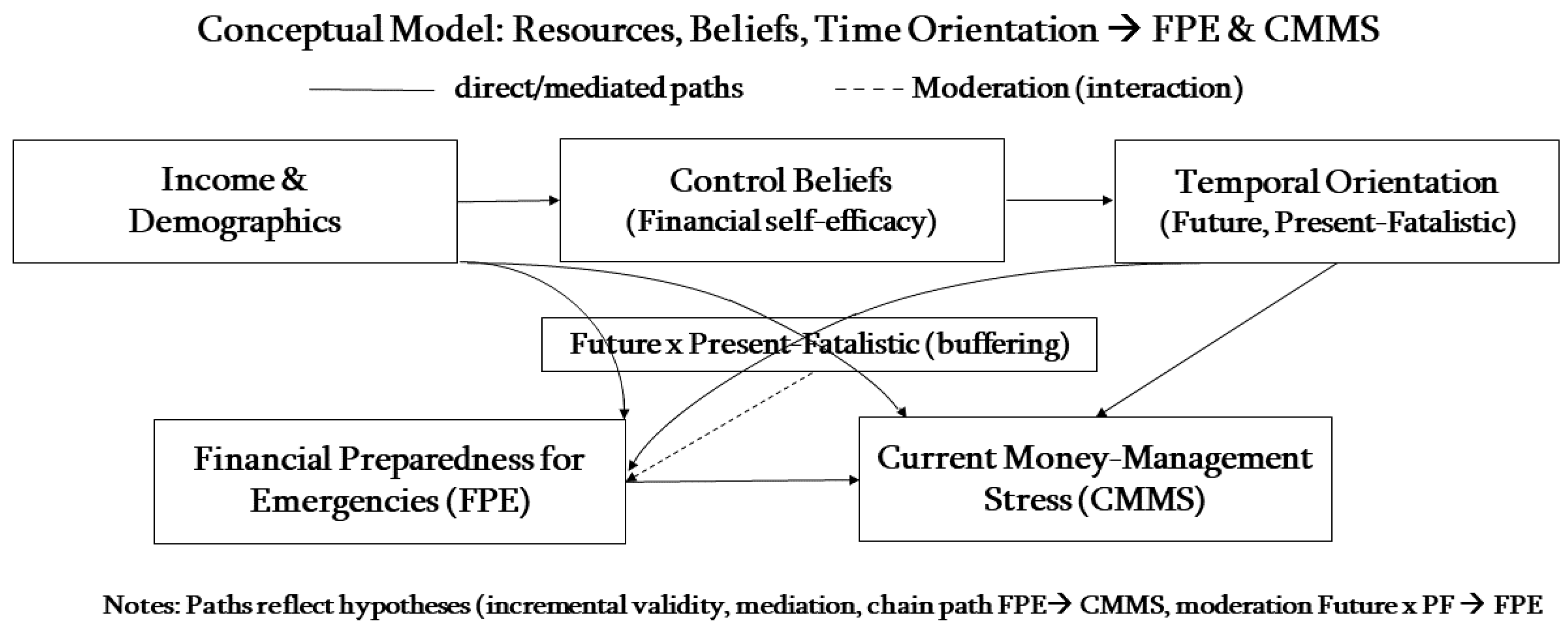
Figure 2.
Standardized Block-2 coefficients with 95% HC3 confidence intervals for FPE and CMMS. Positive values indicate higher preparedness (FPE) or stress (CMMS). After FDR correction, only the Future → CMMS association remained significant.
Figure 2.
Standardized Block-2 coefficients with 95% HC3 confidence intervals for FPE and CMMS. Positive values indicate higher preparedness (FPE) or stress (CMMS). After FDR correction, only the Future → CMMS association remained significant.
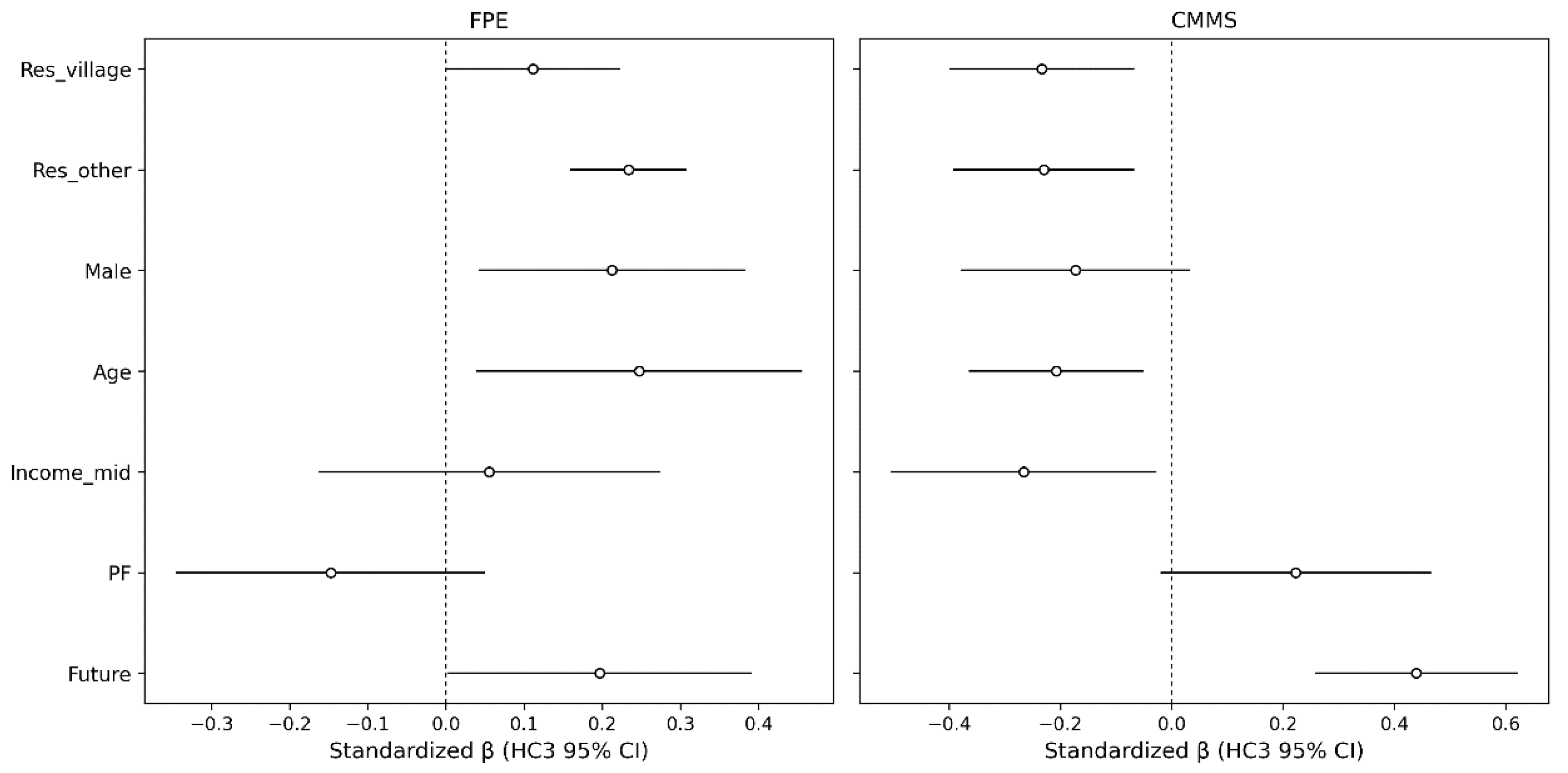
Figure 3.
Marginal-effects plot: Marginal effect of Future on CMMS with covariates set at their means; ribbon shows the 95% HC3 confidence interval. The positive slope was FDR-significant; Present-Fatalistic showed no unique effect on CMMS after correction.
Figure 3.
Marginal-effects plot: Marginal effect of Future on CMMS with covariates set at their means; ribbon shows the 95% HC3 confidence interval. The positive slope was FDR-significant; Present-Fatalistic showed no unique effect on CMMS after correction.
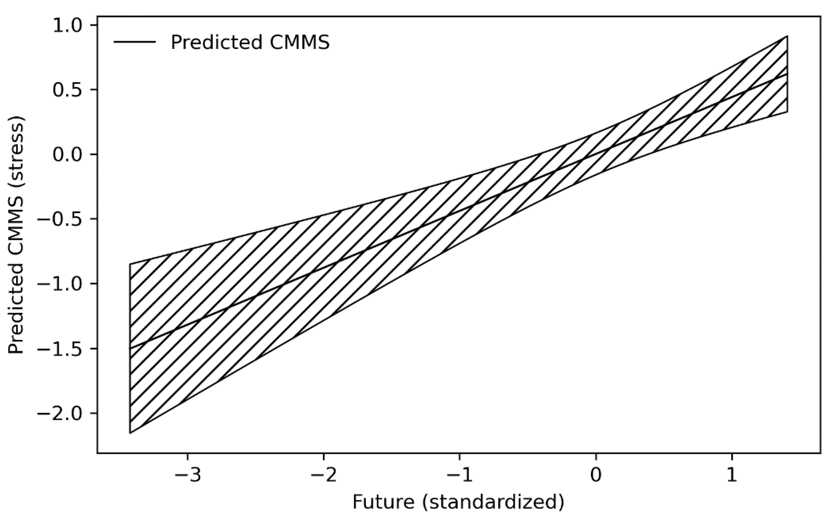
Figure 4.
ΔR² bar chart Incremental variance (ΔR²) from adding Future and Present-Fatalistic to covariates: modest for preparedness (FPE; ΔR² ≈ .06) and meaningful for stress (CMMS; ΔR² ≈ .17). The bars show Block-2 gains over Block-1 models.
Figure 4.
ΔR² bar chart Incremental variance (ΔR²) from adding Future and Present-Fatalistic to covariates: modest for preparedness (FPE; ΔR² ≈ .06) and meaningful for stress (CMMS; ΔR² ≈ .17). The bars show Block-2 gains over Block-1 models.
Disclaimer/Publisher’s Note: The statements, opinions and data contained in all publications are solely those of the individual author(s) and contributor(s) and not of MDPI and/or the editor(s). MDPI and/or the editor(s) disclaim responsibility for any injury to people or property resulting from any ideas, methods, instructions or products referred to in the content. |
© 2025 by the authors. Licensee MDPI, Basel, Switzerland. This article is an open access article distributed under the terms and conditions of the Creative Commons Attribution (CC BY) license (http://creativecommons.org/licenses/by/4.0/).
Copyright: This open access article is published under a Creative Commons CC BY 4.0 license, which permit the free download, distribution, and reuse, provided that the author and preprint are cited in any reuse.


