
Submitted:
30 October 2025
Posted:
31 October 2025
You are already at the latest version
Abstract
The aim of this study is to quantify the impact of increased surface solar radiation on climate warming in Central Europe from 1915-2024 and to re-examine the relationship between CO2 concentrations and global CO2 emissions. A statistical model with proxies for short-wave and long-wave radiation (sunshine duration SSD and CO2 concentration) as independent variables and surface air temperature as the dependent variable was tested for validity and significance, and the results were presented for six long-term measuring stations in Central Europe. A lifetime concept was evaluated for CO2 concentration and contrasted with the concept of accumulated CO2 emissions. The statistical model fulfilled all tests (error probability, normal distribution of the residuals, autocorrelation, statistical power, multicollinearity) and showed that the increase in SSD in the entire year accounts for around 20% of the warming over the last 100 years, in the summer half-year (April-September) and summer (June-August) it is around 30%. The increase in CO2 concentration accounts for the remainder portion of warming of 70-80%. Studies and models neglecting the influence of the increase in surface solar radiation are overestimating the influence of GHG on warming. The development of CO2 concentrations from industrialization until today can be mapped very well with a lifetime of 58 years. Therefore, reducing annual CO2 emissions by around half would stabilize CO2 concentrations.
Keywords:
climate change
; surface air temperature
; global radiation
; sunshine duration
; CO2 emissions
; CO2 air concentration
1. Introduction
There are many studies on the long-term variations of surface solar radiation (SSR) referred to as global dimming and brightening. Basically, this variability is derived from different radiative transmittances of the atmosphere; the latter is significantly influenced by direct and indirect (cloud-related) radiative aerosol effects.
CHERIAN et al. (2014) have used observations and climate model simulations from the Fifth Coupled Model Intercomparison Project (CMIP5) archive to infer clues about the global climate forcing by anthropogenic aerosols. It turned out that solar brightening had strongly contributed to European warming since the mid-1980s.
RUCKSTUHL et al. (2008) showed solar brightening under clear sky conditions with aerosol optical depth (AOD) measurements at some radiation sites in Germany and Switzerland. The measurements confirmed solar brightening between 1986 and 2005 indicating that the direct aerosol effect had an approximately five times larger impact on climate forcing than the in-direct aerosol and other cloud effects.
JIAO et al. (2024) set up a reasonable partial convolutional neural network model based on the global reanalysis data set (20CRv3) to distinguish the effects of cloud cover and aerosols on the decadal variations of surface solar radiation (SSR) from 1961-2018 in the Northern Hemisphere. It turned out, that variations of NH3, SO2 and NOx are important drivers for the inter-decadal SSR variations. There are considerable discrepancies between similar studies on that topic.
Already nearly 30 years ago, SCHWARTZ (1996) stated that the magnitude of the resulting decrease in absorption of surface solar radiation due to aerosols is estimated to be comparable on global average to the enhancement in infrared forcing at the tropopause due to increases in concentrations of CO2 and other greenhouse gases over the same time period.
Increasing SSR due to decreasing aerosol loads are not restricted to Central Europe. MATEOS et al. (2013) e.g., detected a statistically significant linear trend of the mean annual cloud and aerosol radiative effect series over Spain from 1985-2010 of +3.1 W/m2 per decade.
TEN BRINK et al. (2012) addressed the magnitude of the regional first aerosol indirect forcing effect (AIE) with two different approaches: Modelling based on a generic parameterization of the interaction of aerosols and clouds (Chemical Transport Model LOTOS-EUROS and regional climate model RACMO2) and experimentally testing of the cloud forming proper-ties of the regional aerosol in a cloud chamber. The regional manmade aerosol component ammonium nitrate appears to be of equal importance to the magnitude of the AIE as the component sulphate which is normally considered concerning AIE.
The role of nanoparticles in indirect radiative cloud effects has been addressed in various studies. FAN et al. (2018) used observational evidence and numerical simulations to determine an enhancement of the convection and precipitation intensity of tropical clouds by nanoparticles with diameters < 50 nm. KARLSSON et al. (2021) investigated the role of nanoparticles in arctic cloud formation. For large parts of the year, and especially during the dark period, large relative contributions of Aitken mode particles to the cloud residuals were observed. The presented results are thought to be able to improve the representation of low-level clouds in Earth system models.
The studies presented here represent only a small selection of the many investigations into surface solar radiation and the direct and indirect radiation effects of the aerosol. There are still many gaps in knowledge and uncertainties in this field. In this context, a quantitative estimation of the influence of varying global radiation on surface air temperature was con-ducted by THUDIUM AND CHÉLALA (2024) with the help of a multiple linear regression model. It was based on measured monthly values of sunshine duration, global radiation and temperature data from six stations in Switzerland, Austria and Germany from the 1950-2020 period. The increase of global radiation was found to be responsible of half of the warming since the 1980s in the summer half-year (April-September), and of a quarter for the period 1950-2020. For the entire year, the proportion of global radiation on warming was smaller, but still considerable.
This study investigates the influence of surface solar radiation and CO2 air concentration on surface air temperature from 1915 to 2024. Since radiation measurements do not go back that far, the sunshine duration (SSD) was tested as proxy and used over the entire period. By going back to 1915, the brightening phase in the late 1940s is fully captured. By disentangling the temperature influence of SSR and CO2, it is also important to take a new look at the relationship between CO2 concentration and emissions.
Chapter 2 describes the measurement data used. Chapters 3 and 4 discuss the variables SSD and CO2, respectively. Chapter 5 presents the methodology and the results of the multiple linear regression model. Chapter 6 deals with the relationship between CO2 concentration and emissions.
2. Measurements
2.1. Measuring Stations
Monthly data on sunshine duration and temperature from three national meteorological ser-vices (MeteoSchweiz for Switzerland, GeoSphere for Austria and DWD for Germany) from 1895 to 2024 were used in this study. In total, results from four stations from Switzerland, one station from Austria and one from Germany were analyzed. In addition, measurements of global radiation in Potsdam (Germany) since 1947 were used. Selection criteria for the six stations were a good homogenization of data and a position in a relatively flat terrain, so that the sunshine and radiation measurements were not disturbed by slopes. Table 1 shows the coordinates of the stations, and their geographical location is indicated in Figure 1.
As a representative CO2 air concentration, monthly mean carbon dioxide measurements at Mauna Loa Observatory, Hawaii, were used (provided by NOAA Global Monitoring Laboratory, Boulder, Colorado, USA: Dr. Xin Lan, NOAA/GML (gml.noaa.gov/ccgg/trends/) and Dr. Ralph Keeling, Scripps Institution of Oceanography (scrippsCO2.ucsd.edu/)). The carbon dioxide data on Mauna Loa constitute the longest record of direct measurements of CO2 in the atmosphere. They were started by C. David Keeling of the Scripps Institution of Oceanography in March of 1958 at a facility of the National Oceanic and Atmospheric Administration (Keeling, 1976).
2.2. Dataset
For a long time series of meteorological data, traceability is a special challenge. The national meteorological services make serious efforts to homogenize these data. Within the framework of this study, no further adaptations of the data delivered from the national meteorological services were made.
The monthly data of the four Swiss stations (Basel, Bern, Genève, Zürich) for temperature and sunshine duration were homogenized by MeteoSchweiz (Begert et al. 2003; Moesch and Zelenka 2004; Dürr et al. 2016; Scherer and Begert 2019). The sunshine duration and temperature data from these four stations were averaged and named as “Swiss Plateau”.
The monthly data of the German station (Potsdam) for global radiation, temperature and sunshine duration were homogenized by DWD. In particular, the global radiation measurements have been subjected to careful homogenization (as reported by Wild et al. 2021) and regular calibrations have taken place since 1947.
For the Austrian station (Wien), the monthly database of GeoSphere for temperature and sunshine duration was analyzed.
3. Long-Term Development of Sunshine Duration and Global Radiation in Central Europe 1915-2024
Long-term records of sunshine duration (SSD) for Potsdam, Wien and the Swiss Plateau from 1915 – 2024 are showed in Figure 2. Although the differences between the three regions are sometimes considerable, the general trend is well represented by all regions, being representative of most regions in Central Europe not situated at higher elevations. Accordingly, the SSD course between 1915 and around 1970 shows two phases of increased values. The first smaller phase, not occurring in the Swiss Plateau, took place from 1930-1936, the second larger one from 1942-1955. From 1970-1988 was a phase of reduced levels of SSD during the period of highest air pollution in Europe. From about 1975 to around 1988, the SSD was lower than at any other time since the beginning of the 20th century, after which a continuous increase set in until the end of the observation period 2024, reaching the highest values of the last 110 years at all sites of measure. From '1920' (1915-1924) to '2020' (2015-2024), SSD in Central Europe has increased by about 170 h (+14%) in the summer half-year (April-September).
The real driver of temperature effects due to solar radiation is not the duration of the sunshine, but the short-wave solar radiation reaching the ground, i.e. the global radiation (GR). Thudium and Chélala (2024) have already shown that there is a high correlation between global radiation and SSD at the locations under consideration, specific for each location. As the GR measurements do not go back that far, the SSD was used as a proxy. Figure 3 shows the interaction of SSD, GR and cloud cover for the summer (June-August), the summer half-year and the entire year using Potsdam as an example.
GR correlates very well with SSD, for all seasons. In summer, the high SSD peaks are more pronounced than in GR up to around 1980. It is possible that intermittent cloud cover, which is particularly frequent in summer, led to a certain overestimation of sunshine duration with earlier measuring instruments, which could not be compensated for by homogenization (e.g. Sonntag and Behrens 1992).
Overall, the course of SSD shows an increasing phase from 1915-1950, a decreasing phase from 1950-1980 and after 1980 again an increasing phase to the highest values of the last 110 years. The cloudiness modulates the SSD, sometimes significantly, e.g., the peak around 1950 was additionally reinforced by a series of years with relatively few clouds. But the course of the SSD is by no means determined by the cloud cover. Overall, the latter even shows a tendentially increasing trend.
The general increase in SSD (and thus GR) over the last 110 years is due to the overall increasing transparency of the atmosphere, due to changes in the direct and indirect aerosol radiation effects (e.g. Thudium and Chélala, 2024). The direct aerosol radiation effect refers to the scattering and absorption of radiation by aerosol particles outside clouds. The indirect effect refers to the radiation impact of aerosol particles on clouds. Concentration, initial size distribution and chemical composition (e.g. different proportions of mineral dust or sea salt) of the aerosol particles are essential for the resulting spectrum of cloud droplets, influencing e.g. albedo and optical thickness of the clouds.
The dimming phase from 1950 to 1980 and the brightening phase from 1980 to the present were coincident with a sharp increase in air pollution in the PBL (planetary boundary layer) and subsequent air pollution abatement strategies. Increasing air pollution and subsequent purification certainly had an influence on global dimming and brightening; however, the course of SSD can hardly be explained by the course of air pollution in the PBL alone:
The increasing SSD in the first half of the 20th century cannot be explained by decreasing air pollution (see also Figure 2).
An active aerosol component in the short-wave solar spectral range is sulphate, which forms from emitted SO2. Hoesly and Smith (2024) and Hoesly et al. (2018) have evaluated global SO2 emissions from the 18th century to the present. The formation of sulphate occurs quite slowly, during many hours to days, so that the sulphate is spread over a wide range in the PBL and even in the whole troposphere. According to this, SO2 emissions in Europe (as a proxy for sulphate) at the end of the 19th century were about the same as today, so the sulphate cannot explain the current brightening compared to the years around 1900. JIAO et al. (2024) and TEN BRINK et al. (2012) found other compounds than sulphate with similar influence on surface solar radiation and therefore SSD (s. introduction). The development of dust and soot (from 1900 - 2010 similar to SO2) can also hardly explain the course of SSD.
Further information is provided by the development of direct solar radiation (DSR) on the ground for cloud-free and cloudy skies near Potsdam from 1947-2024 (Figure 4; see also Thudium and Chélala 2024).
Global dimming from around 1950-1980 and global brightening thereafter are clearly recognizable. Two aspects are important for this discussion:
1. Direct solar radiation (DSR) has been increasing continuously in the cloud-free situation since 1980, i.e., the opacity of the atmosphere in the short-wave spectral range in the absence of clouds has been decreasing continuously until today; this does not correspond to the reduction path of SO2 in the PBL (strong decrease from 1980-2000, small decrease from 2000-2020).
2. Direct solar radiation under cloudy skies shows the same relative trend as cloud-free sky until around 1995. Thereafter, the relative increase is slight at first, and from around 2010 onwards significantly greater than under cloudless skies. The light transmission of clouds has therefore also increased, which typically happens with fewer but larger droplets.
Although the relative DSR increase is greater under cloudy skies than under cloudless conditions, the absolute DSR increase is nevertheless greatest under cloudless skies (approximately +50 W/m² for the summer half-year on a 24-hour average from 1980-2022).
In summary, it can be stated that the reasons for the course of SSD over the last 110 years have not been completely clarified yet.
4. Long-Term Development of CO2 Air Concentration 1895-2024
The second independent variable in our regression model is the CO2 air concentration. The CO2 values from Mauna Loa are only a little bit higher than the global average calculated by NOAA since 1979. "The NOAA GML Carbon Cycle Group computes global mean surface values using measurements of weekly air samples from the Cooperative Global Air Sampling Network (Conway et al., 1994; Dlugokencky et al., 1994; Novelli et al., 1992; Trolier et al., 1996). The global estimate is based on measurements from a subset of network sites. Only sites where samples are predominantly of well-mixed marine boundary layer (MBL) air representative of a large volume of the atmosphere are considered. These “MBL” sites are typically at remote marine sea level locations with prevailing onshore winds. Measurements from sites at altitude (e.g., Mauna Loa) and from sites close to anthropogenic and natural sources and sinks are excluded from this global estimate." (Quoted from https://gml.noaa.gov/ccgg/about/global_means.html. See there for more details.)
The data from Mauna Loa go back 20 years longer than the global means described above. For the period 1895-1957, the CO2 trend was estimated by extrapolating the polynomial ap-proximation from 1958-2024 to 1895. Around 1895, CO2 was at the pre-industrial level of 280 ppm. Figure 5 shows the annual means of measurements from Mauna Loa 1958-2024, the global means from 1979-2024 and the extrapolation for 1895-1957.
5. Methodological Approach
The surface air temperature is the result of many complex processes such as increasing GHG-concentrations, changing circulations in oceans and air, changes in sunshine duration SSD and other parameters, most of them not linear with time. All these processes are governed by the fact that the Earth system gains or loses heat energy through radiation processes. Shortwave radiation incident on the Earth's surface is global radiation, the change in which is measured directly or determined using the SSD as proxy (see chapter 3). The change in long-wave radiation is largely determined by the change in atmospheric concentrations of greenhouse gases, with CO2 as a proxy (see chapter 4). Other greenhouse gases are also included in the proxy CO2 insofar as their changes run proportional to fossil CO2 changes, i.e. fossil methane and parts of N2O emissions. Not included are changes in biogenic emissions of CO2 and methane, as they do not run parallel to fossil CO2 (relevant for global warming from 1920 to 2020 are only changes e.g. in wood combustion or livestock farming between 1920 and 2020).
Therefore, as methodological approach of choice we set up a multiple linear regression as statistical model with temperature as the dependent variable and SSD and CO2 as independent variables. Each model application had to be tested of statistical significance, i.e. if the two independent variables were enough to describe the course of the dependent variable (s. below). The model was based on yearly and seasonal values from the period 1915-2024. The regression model was started only in 1915 because the uncertainty of SSD increases the further the measurements lie in the past. The homogenization of the series of measurements of relative sunshine duration at the stations of Bern and Geneva from MeteoSwiss resulted in confidence intervals that were about twice as wide before 1915 (Bosshard 1996). Other factors not covered by SSD and CO2, as e.g. albedo or further GHG's, may also influence temperature. These influences are included in the statistical error; statistical tests (s. below) show whether the error is small enough for statistical statements.
Although our multi-linear regression approach with two independent variables omits non-linear effects and other complexities of the climate system, we ensure its general applicability by a set of five statistical standard tests. The tests for the approach in this study are described as follows (s. Thudium and Chélala 2024 for more details):
T1: determined regression coefficients for SSD and CO2 are significant (error probability p<0.05).
T2: Shapiro-Wilk Test for normal distribution of the residuals, i.e., the linear relation of temperature with SSD as well as with CO2 is adequate. Based on convention the test value must be >0.05.
T3: Durbin-Watson test for autocorrelation (correlation inside the dependent variables). This can be a problem especially for the correlation of time series. The accepted range of the Durbin-Watson test value was between 1.5 and 2.5 (for n=110 values per regression (years) and an alpha level a=0.01).
T4: Statistical power (likelihood that a model detects an existing effect), depending on r² of the regression. Based on convention the statistical power must be >0.80, the maximum value is 1.
T5: Variance Inflation Factor (VIF) to measure multicollinearity of the independent variables, or of the linear combination of the independent variables in the regression. In the present model, SSD and CO2 are the independent variables. SSD could be dependent on CO2 (structural multicollinearity) or the effect of SSD on temperature could be dependent on CO2 (sample-based multicollinearity). The VIF is calculated regarding both types of multicollinearity. A value of 1 means no multicollinearity; VIF values above 4 suggest possible multicollinearity; values above 10 indicate serious multicollinearity.
The model was run for the laps of time of year, summer half-year (April to September) and summer (June to August) mean values for the three sites Potsdam, Wien and Swiss Plateau, totally 9 regressions. A regression result was only used to determine the influence of SSD and CO2 on surface air temperature if all five tests were fulfilled, i.e., if only one test was not fulfilled, no result could be given.
The regression period 1915-2024 includes phases of global brightening and of global dimming. The coefficients expressing the impact of SSD respective CO2 on temperature are valid for the whole period.
6. Results
All nine regression models were successful, i.e. each fulfilled all five statistical tests. In summary, the test results were as follows:
T1: Significance of regression coefficients for SSD and CO2 (error probability p<0.05): It was always p< 10-5, in the average p=7*10-7 for SSD and p=4*10-14 for CO2.
T2: Shapiro-Wilk Test for normal distribution of the residuals, test value must be >0.05: test value was between 0.2 and 0.9 with an average of 0.5.
T3: Durbin-Watson test for autocorrelation (correlation inside the dependent variable). The test value should be between 1.5 and 2.5, it was from 1.62 to 1.82 with an average of 1.70.
T4: Statistical power (likelihood that a model detects an existing effect), must be >0.80, the maximum value is 1. In all regressions the statistical power was 1.
T5: Variance Inflation Factor (VIF) to measure multicollinearity of the independent variables. Factor should be near to 1, in any case <4. It was 1.01 to 1.31 with an average of 1.09. The result of this test has a special meaning for this regression model: It means that the amount of SSD over the entire epoch has not been influenced by CO2, and that the temperature effect of SSD is independent of the development of CO2. SSD and CO2 are therefore independent drivers of global warming in Central Europe.
Thus, all regressions fulfilled the tests and led to significant results. Figure 6 shows the results of the regression model: the measured and estimated mean temperatures for the entire year, the summer half-year and the summer for the three sites. The measured temperature curves are well represented by the estimate at all locations, in particular the global dimming and brightening phases are mapped quite precisely: The temperature course from 1915-2024 can be expressed by CO2 and SSD, whereby all influences not represented by CO2 or SSD account for a temperature effect of ±0.3 °C based on 5-year averages (standard error, see Table 2). The temporary warming in the 1940s with accumulation 1945-1950 is not fully shown in the estimate, possibly because of major weather patterns or ocean circulations.
The behavior of measured and estimated temperatures is very similar at all three sites. Therefore, climate warming in Central Europe, with all its complex processes and feedback, can essentially be represented by the two variables CO2 concentration and SSD.
Table 2 shows the regression coefficients for SSD and CO2 as well as the standard error of the estimated temperatures (of the yearly values and of the 5-year averages) for the entire year, the summer half-year and the summer, averaging over the three sites Potsdam, Vienna and Swiss Plateau.
The regression model allows the influence of SSD and CO2 on climate warming in Central Europe over the last 100 years to be apportioned. The difference between the mean values of SSD and CO2 between ‘1920’ (1915-1924) and ‘2020’ (2015-2024) multiplied by the regression coefficients for SSD and CO2 gives the respective contribution of the change in SSD and CO2 to the warming between ‘1920’ and ‘2020’. Table 3 shows the results for the entire year, the summer half-year and the summer, as mean values over all three locations.
The increase in SSD in the entire year accounts for around 20% of the warming over the last 100 years, in the summer half-year and summer it is around 30%. In the brightening period 1980-2024, SSD counts for about half of the climate warming. SSD, actually global radiation, for which SSD is a proxy, is therefore a driver of warming that should not be ignored.
The increase in CO2 concentration accounts for the remainder portion of warming of 70-80%, mainly caused by fossil CO2 emissions, and to a lesser extent by changes in land use.
In summary, the results of the regression model have shown that there is a linear relationship between atmospheric CO2 concentration (above 280 ppm, the value at the beginning industrialization) and global warming induced by it, being 70-80% of total warming. In Central Europe this was about 0.015 °C/ppm CO2 over the whole period 1915-2024. This linearity is no longer disturbed by global dimming and brightening effects, as the latter are represented in a separate term.
Given the postulated logarithmic relationship between CO2 concentration and radiative forcing, some model runs with the logarithmic values of CO2 concentrations were also performed. The results (model test coefficients, r², standard errors of the residuals, coefficient of SSD and portion of warming to be attributed to SSD and CO2, respectively) were nearly identical to the results with absolute CO2 values.
As mentioned in Chapter 3, global radiation has increased under both cloudless and cloudy skies. Since around 1995, it has increased more in percentage terms under cloudy skies (Thudium and Chélala 2024). This must have to do with indirect aerosol radiation effects.
7. Discussion of the Concept of Cumulative CO2 Emissions
The increase in CO2 concentration since the beginning of industrialization was caused by the emission of fossil carbon. In the years 2009-2013, an almost linear relationship was established between cumulative CO2 emissions and the resulting global warming, which was reflected in the IPCC's AR5. The amount of global warming per unit of cumulative carbon dioxide emissions (°C/Gt CO2) is referred to as the transient climate response to cumulative CO2 emissions (TCRE). This TCRE relationship has been used to estimate the amount of CO2 emissions that would be consistent with limiting global warming to a certain threshold, the so-called 'remaining carbon budget'. Various studies agree that the approximate constancy of the TCRE (i.e. its independence from cumulative CO2 emissions) would result from the trade-off between the decreasing equilibrium sensitivity of radiative forcing to CO2 at higher atmospheric concentrations and the decreasing ability of the ocean to absorb heat and carbon at higher cumulative emissions (s. Canadell et al., 2021: Chapter 5 of IPCC AR6). Here, a new look at this relationship is taken.
7.1. Lifetime Concept for CO2 Air Concentration
In a first step, we like to develop a lifetime concept for the resulting CO2 air concentration. The yearly fossil CO2-emissions worldwide since 1960 have been evaluated in the Global Carbon Project GCP (Andrew and Peters, 2023; Friedlingstein et al., 2023; Peters et al., 2011). The CO2 air concentration is represented by the Mauna Loa measurements since 1958, extrapolated backwards until 1895 (s. chapter 4). Based on this extrapolation, we also estimated the yearly fossil CO2-emissions backwards until 1895.
The CO2 in the atmosphere interacts with oceans and land. Fossil CO2 is obviously stored by both reservoirs, so that only a portion of the emissions remain in the atmosphere. In 2023, the total fossil CO2 emitted from 1960-2023 amounted to 1514 Gt (1514*1012 kg) or 412.9 Gt C according to the GCP. From 1895-2023, with the backwards extrapolation mentioned above, the total fossil CO2 emissions amounted to 1962 Gt or 535.1 Gt C, and the global atmospheric CO2 concentration increased by an average of 141.1 ppm (Mauna Loa database). The carbon content of the atmosphere increases by 2.12 Gt C per ppm of additional CO2 concentration (e.g. Heimann, 2022; Archer et al., 2009), so 299.1 Gt C were 'needed' to reach the amount of 141.1 ppm CO2 over the preindustrial level. This is 56% of the total fossil C emitted into the atmosphere from 1895-2023, i.e. all fossil C emitted since the beginning of industrialization. The remaining 44% were taken up by oceans and land until 2023.
When a transfer of a substance from one place to another is driven by a difference in concentration or intensity, a concept of lifetime is often suitable for description. In this case, lifetime does not mean the average time of existence of a (radioactive) atom or molecule, but the lifetime of the additional concentration in the atmosphere due to fossil emissions.
Of course, the lifetime concept for CO2 cannot apply over thousands of years, because then other processes become more important for the uptake of CO2 by oceans and land. However, if the concept yields good results for the last 130 years (see below), it can be postulated as an empirical model for another about 100 years.
If t is the lifetime (time in which the concentration drops to 1/e), then the CO2 emission remaining in the atmosphere in year t is:
E(t) = [E(t-1) + e(t)] * e-1/t
with E(t) or E(t-1): Emission remaining in the atmosphere in year t or in the previous year.
e(t): Emission in year t.
It is a lifetime of 58 y that leads to the mentioned 56% remaining emissions in 2023 and indicates the actual remaining emissions in each year. Figure 7 shows the development of CO2 airborne concentration and the emissions remaining in the atmosphere for a lifetime of 58 years for the period 1960-2023. The emissions remaining in the atmosphere with a lifetime of 58 years describe the course of CO2 concentration extraordinarily well (r² = 0.9996). Apparently, the uptake conditions of oceans and land remained very stable throughout the entire period.
The lifetime of 58 y means that 37% of the emissions of a given year are still present after 58 years and 18% after 100 years. This was the reality of the last 130 years.
7.2. Discussion of Accumulated CO2 Emissions
The accumulated CO2 emissions (Eacc) correlate also very well with the course of CO2 concentration (s. Figure 7). The fact that the CO2 concentration increase (Dc) is proportional to the remaining emissions (ER), is clear, and that the latter correspond to a lifetime of 58 years can be understood. But why the CO2 concentration increase is also proportional to the accumulated emissions, a virtual quantity not existing in the atmosphere?
There are two proportionalities:
Eacc ~ Dc and Eacc ~ DT (climate warming).
These proportionalities mandatorily imply the following third proportionality:
Dc ~ DT according to the findings of our statistical model.
Because Dc ~ ER, it is also Eacc ~ ER, i.e. Eacc = a*ER (a=constant) for each year. ER is the result of many lifetime processes (for each year), so Eacc can only be proportional to ER if
Eacc(t) = b*E(t) for each year. This is the case: Over the entire period, there is a linear relationship between the annual CO2 emissions and the accumulated emissions up to that time point (with r²=0.97; see Figure 8). There are purely mathematical reasons why the accumulated emissions - if the y-axis is scaled accordingly - also reflect the CO2 trend well in Figure 7. When the annual CO2 emissions are no more proportional to the accumulated emissions (in case of stabilization and even reduction of the annual emissions), the CO2 concentration (and thus climate warming) will no longer be in a linear relationship to the accumulated emissions but will still be described by the lifetime concept. Consequently, the concept of lifetime appears to be more suitable to describe the future development of CO2 in the atmosphere than the concept of accumulated CO2 emissions with a "remaining emission budget".
If global yearly emissions are reduced in the relatively near future so that they come in the range of the 'loss' of the CO2 content of the atmosphere as a result of transfers to land and oceans (about half of an actual yearly emission), the CO2 concentration will be stabilized, in line with the development of the last 130 years. Further reductions will lead to lower CO2 concentrations. However, the climate would be significantly warmer than at the corresponding CO2 concentration in the past due to the warmer oceans, lower albedo and increased solar radiation on the ground. The temperature response depends essentially on the balance of carbon sinks and ocean heat uptake (MacDougall et al., 2020). Furthermore, the acidification of the oceans would continue. So there is no way around the need for a rapid reduction in worldwide fossil carbon emissions to the half in a first step. In the further future the lifetime may be extended, especially if the storage capacities of the oceans would be reduced, e.g. as a result of warming or strengthening of stratification (Roch et al., 2023).
Some persistent residues above pre-industrial concentration will remain in any case, which will only be reduced very slowly. Mixing CO2 with deep layers of the oceans will take several hundred years, while sedimentation and rock weathering will take thousands of years (e.g. Brovkin and Gayler, 2022).
7.3. Comparison of CO2 Concentration Decays in Models Presented in IPCC AR5 und AR6 with the Lifetime Concept
The decay of the CO2 concentration in the atmosphere due to interactions in the Earth system (land, ocean) has already been investigated in many models (e.g. Archer et al., 2009; Ciais et al., 2013 (Chapter 6 in IPCC AR5); Brovkin and Gayler, 2022). A pulse was given in model year 0 and modeled how the CO2 concentration changes over time. According to these models, the CO2 concentration also falls markedly in the first decades (as modulated exponential functions), but less sharply than with a lifetime of 58 y (Joos et al. 2013). The real emissions can also be imagined as a sequence of 130 pulses that overlap. In the illustration by Ciais et al., 2013 (Box 6.1, Figure 1 in Chapter 6 of IPCC AR5), 60 years after the release of the CO2 pulse, depending on the model, 32-60% of CO2 are still present in the atmosphere (36% in reality over the last 130 years), 28-54% after 100 years (18% in real terms). These exponential decay rates can be compared with corresponding lifetimes: 32-60% after 60 years correspond to lifetimes of 53-117 y; 28-54% after 100 years correspond to lifetimes of 79-162 y. In the first half of the century after the pulse the models showed a range of same decay as present in reality until half of it, in the second half, further reductions in CO2 uptake by the ocean and land mass were assumed.
The decay of atmospheric CO2 concentration due to ocean and land mass uptake is very crucial for climate evolution after a cessation of CO2 emissions (Zero Emissions Commitment ZEC). In the IPCC AR6, the results of 20 models were shown that simulated the evolution of CO2 and the response of the Earth's surface temperature after cessation of CO2 emissions for an experiment in which 1000 Gt C are emitted during a continuous increase in atmospheric CO2 concentration of 1 % / year (Jones et al., 2019; MacDougall et al., 2020). All simulations showed a strong decrease in atmospheric CO2 concentration after CO2 emissions cease, in line with previous studies and the basic theory that natural carbon sinks persist (Fig. 4.39 in Chapter 4 of IPCC AR6). Therefore, according to AR6, there is high confidence that atmospheric CO2 concentrations will decrease for decades when CO2 emissions cease (s. Lee et al., 2021: Chapter 4 of IPCC AR6).
The project described in the section above was replicated on the basis of a lifetime of 58 years. After 73 years, the 1000 Gt C had been emitted with a maximum CO2 concentration of 579 ppm. This was comparable with other models (e.g. MacDougall and Knutti, 2016: c max=540 ppm after 65 years). However, the subsequent decrease in CO2 was considerably faster than postulated by the models: After 60 years from the start of zero emissions, 62-78% of the initial concentration of CO2 were still present in the models, corresponding to a lifetime of 120-240 years. After 100 years, 53-74% were still present, corresponding to a lifetime of 160-330 years. Of course, the approach only on the basis of a lifetime of 58 years for the first century after the start of zero emissions is simple, but it corresponds to the real course of atmospheric CO2 over the last 130 years. In the models, immediately after the end of CO2 emissions, the lifetime increases several times over. The discrepancies within the 20 models and also in comparison to the model results of the theoretical 'pulse experiments' (see above) are large.
8. Conclusions
According to the model results, 20-30% of the warming since the beginning of industrialization can be assigned to the increase in SSD. This is a considerable proportion, which has a particularly strong effect in already radiation-rich situations in summer. Increased drying out of the soil (evapotranspiration) due to increased radiation absorption, increased heat stress in the case of a lack of radiation protection, increased intensity of urban heat islands, more frequent and more intensive short-term extreme precipitation (where a lot of energy has to accumulate in a short time) are consequences to be considered. In such situations, the additional energy (compared to the 1980s) due to the increased short-wave irradiation is much higher than that due to the increased long-wave back radiation as a result of the increased GHG concentrations. Generally, the contribution of SSD (as proxy for surface solar radiation) has implications for climate mitigation and adaptation strategies and might affect regional climate projections.
Studies and models neglecting the influence of the increase in solar radiation are overestimating the influence of GHG on warming. The situation in Europe may be different on other continents and over oceans, because of different occurrences of dimming and brightening effects. But brightening effects have been detected at many locations outside Europe (e.g. Ohmura, 2009; Mortier et al., 2020).
Increased solar radiation is absorbed even more by the ocean than by the land, as its albedo is significantly lower. The contribution of increased solar radiation to ocean warming can therefore be considerable.
The development of CO2 concentrations from industrialization until today (as a driver of global warming) can be mapped very well with a lifetime of 58 years. This means that reducing annual CO2 emissions by around half would stabilize CO2 concentrations and thus also global warming in the medium term (of course, further reductions would be necessary). In contrast, the concept of accumulated CO2 emissions requires ‘zero emissions' for stabilization, and consequently there is a static budget for emissions that are still possible to comply with a certain temperature limit.
This latter concept is correct as long as annual CO2 emissions grow linearly with accumulated emissions, but what about stabilized and reduced (worldwide) annual CO2 emissions, i.e., the phase that humanity will hopefully enter soon? A concept based on lifetime therefore seems to be better suitable for representing the medium-term future.
In models for the course of CO2 concentrations after 'zero emissions' presented in IPCC AR5 and AR6, the factual lifetimes were nevertheless significantly longer than in reality to date, although the accumulated model emissions were smaller than in reality. Against this background, it seems sensible to include the real CO2 development when estimating the future evolution, in the sense that the models for the future should also be able to depict the past.
Author Contributions
The study conception and design were set up by Jürg Thudium. Data collection and presentation were performed by Carine Chélala. All authors contributed to the analysis. The first draft of the manuscript was written by Jürg Thudium and both authors commented on previous versions of the manuscript. Both authors read and approved the published version of the manuscript.
Funding
The Oekoscience Institute fully funded this study.
Data Availability Statement
The datasets (monthly values) analyzed during the current study are available as follows: Switzerland: Homogenized data of temperature and precipitation are available by https://www.meteoschweiz.admin.ch/home/klima/schweizer-klima-im-detail/homogene-messreihen-ab-1864.html. Homogenized data of sunshine duration and global radiation have to be purchased by https://www.meteoschweiz.admin.ch/home/service-und-publikationen/produkte.subpage.html/de/data/products/2014/bodenstationsdaten.html or may be available from the authors upon reasonable request if permitted by MeteoSchweiz. Austria: Meteorological data as temperature, sunshine duration and global radiation are available by https://data.hub.geosphere.at/dataset/. Germany: Homogenized data of temperature, sunshine duration and global radiation are available by https://opendata.dwd.de/climate_environment/CDC/.
Acknowledgments
Data of CO2 concentrations at Mauna Loa Observatory, Hawaii, were provided by NOAA Global Monitoring Laboratory, Boulder, Colorado, USA (https://gml.noaa.gov). We appreciate the support of MeteoSwiss and GeoSphere Austria in the field of global radiation measurements.
Conflicts of Interest
The authors have no relevant financial or non-financial interests to disclose.
Abbreviations
The following abbreviations are used in this manuscript:
| AOD | Aerosol optical depth; |
| GHG | Greenhouse gases; |
| GR | Global radiation; |
| Direct SR | Direct solar radiation; |
| Diffuse SR | Diffuse solar radiation; |
| SSD | Sunshine duration; |
| DWD | National German weather services; |
| GeoSphere | National Austrian weather services; |
| MeteoSwiss: | National Swiss weather services. |
References
- ANDREW, R.M. AND PETERS, G.P. (2023): The Global Carbon Project's fossil CO2 emissions dataset. [CrossRef]
- Archer, D. Eby, V. Brovkin, A. Ridgwell, L. Cao, U. Mikolajewicz, K. Caldeira, K. Matsumoto, G. Munhoven, A. Montenegro, K. Tokos, 2009: Atmospheric lifetime of fossil-fuel carbon dioxide. Annual Review of Earth and Planetary Sciences Volume 37. [CrossRef]
- BEGERT, M., G. SEIZ, T. SCHLEGEL, M. MUSA, G. BAUDRAZ, M. MOESCH, 2003: Homogenisierung von Klimamessreihen der Schweiz und Bestimmung der Normwerte 1961-1990. MeteoSchweiz, Schlussbericht des Projektes NORM90, 170p.
- BOSSHARD, W. , 1996: Homogenisierung klimatologischer Zeitreihen, dargelegt am Beispiel der relativen Sonnenscheindauer. Veröffentlichungen der Schweizerischen Meteorologischen Anstalt, Volume 57.
- BROVKIN, V., V. GAYLER, 2022: Rückkopplungen zwischen Klima und globalem Kohlenstoffkreislauf. Deutscher Wetterdienst, promet, Heft 105, 61–68. [CrossRef]
- CANADELL, J.G. M.S. MONTEIRO, M.H. COSTA, L. COTRIM DA CUNHA, P.M. COX, A.V. ELISEEV, S. HENSON, M. ISHII, S. JACCARD, C. KOVEN, A. LOHILA, P.K. PATRA, S. PIAO, J. ROGELJ, S. SYAMPUNGANI, S. ZAEHLE, AND K. ZICKFELD, 2021: Global Carbon and other Biogeochemical Cycles and Feedbacks. In Climate Change 2021: The Physical Science Basis. Contribution of Working Group I to the Sixth Assessment Report of the Intergovernmental Panel on Climate Change [MASSON-DELMOTTE, V., P. ZHAI, A. PIRANI, S.L. CONNORS, C. PÉAN, S. BERGER, N. CAUD, Y. CHEN, L. GOLDFARB, M.I. GOMIS, M. HUANG, K. LEITZELL, E. LONNOY, J.B.R. MATTHEWS, T.K. MAYCOCK, T. WATERFIELD, O. YELEKÇI, R. YU, AND B. ZHOU (EDS.)]. Cambridge University Press, Cambridge, United Kingdom and New York, NY, USA, pp. 673–816. [CrossRef]
- CHERIAN, R. QUAAS, M. SALZMANN, AND M. WILD, 2014: Pollution trends over Europe constrain global aerosol forcing as simulated by climate models, Geophys. Res. Lett., 41, 2176–2181. [CrossRef]
- CIAIS, P. SABINE, C., BALA, G., BOPP, L., BROVKIN, V., CANADELL, J., CHHABRA, A., DEFRIES, R., GALLOWAY, J., HEIMANN, M., JONES, C., LE QUÉRÉ, C., MYENI, R.B., PIAO, S., THORNTON,P., 2013: Carbon and other biogeochemical cycles. In: Climate Change 2013: The Physical Science Basis. Contribution of Working Group I to the Fifth Assessment Report of the Intergovernmental Panel on Climate Change. STOCKER, T.F., QIN, D., PLATTNER, G.-K., TIGNOR, M., ALLEN, S.K., BOSCHUNG,J., NAUELS, A., XIA, Y., BEX, V., MIDGLEY, P.M. (HRSG.). Cambridge University Press, Cambridge, United Kingdom und New York, NY, USA, 465-570.
- CONWAY, T.J. P. TANS, L.S. WATERMAN, K.W. THONING, D.R. KITZIS, K.A. MASARIE, AND N. ZHANG, 1994: Evidence for interannual variability of the carbon cycle from the NOAA/CMDL global air sampling network, J. Geophys. Res., 99, 22831-22855.
- DLUGOKENCKY, E.J., L. P. STEELE, P.M. LANG, AND K.A. MASARIE, 1994: The growth rate and distribution of atmospheric methane, J. Geophys. Res., 99, 17,021-17,043.
- DÜRR, B., D. SCHUMACHER, M. BEGERT, D. VAN GEIJTENBEEK, 2016: Globalstrahlungsmessung im A-NETZ – Update der Bearbeitung bis zum SMN-Übergang. Fachbericht MeteoSchweiz 262, 30 p.
- FAN, J., D. ROSENFELD, Y. ZHANG, S. GIANGRANDE, Z. LI, L. T. MACHADO, S. MARTIN, Y. YANG, J. WANG, P. ARTAXO, H. M. J. BARBOSA, R. C. BRAGA, J. M. COMSTOCK, Z. FENG, W. GAO, H. B. GOMES, F. MEI, C. PÖHLKER, M. L. PÖHLKER, U. PÖSCHL, R. A. F. DE SOUZA, 2018: Substantial convection and precipitation enhancements by ultrafine aerosol particles. Science 359, 411–418. [CrossRef]
- FRIEDLINGSTEIN, P. O'SULLIVAN, M., JONES, M. W., ANDREW, R. M., BAKKER, D. C. E., HAUCK, J., LANDSCHÜTZER, P., LE QUÉRÉ, C., LUIJKX, I. T., PETERS, G. P., PETERS, W., PONGRATZ, J., SCHWINGSHACKL, C., SITCH, S., CANADELL, J. G., CIAIS, P., JACKSON, R. B., ALIN, S. R., ANTHONI, P., BARBERO, L., BATES, N. R., BECKER, M., BELLOUIN, N., DECHARME, B., BOPP, L., BRASIKA, I. B. M., CADULE, P., CHAMBERLAIN, M. A., CHANDRA, N., CHAU, T.-T.-T., CHEVALLIER, F., CHINI, L. P., CRONIN, M., DOU, X., ENYO, K., EVANS, W., FALK, S., FEELY, R. A., FENG, L., FORD, D. J., GASSER, T., GHATTAS, J., GKRITZALIS, T., GRASSI, G., GREGOR, L., GRUBER, N., GÜRSES, Ö., HARRIS, I., HEFNER, M., HEINKE, J., HOUGHTON, R. A., HURTT, G. C., IIDA, Y., ILYINA, T., JACOBSON, A. R., JAIN, A., JARNÍKOVÁ, T., JERSILD, A., JIANG, F., JIN, Z., JOOS, F., KATO, E., KEELING, R. F., KENNEDY, D., KLEIN GOLDEWIJK, K., KNAUER, J., KORSBAKKEN, J. I., KÖRTZINGER, A., LAN, X., LEFÈVRE, N., LI, H., LIU, J., LIU, Z., MA, L., MARLAND, G., MAYOT, N., MCGUIRE, P. C., MCKINLEY, G. A., MEYER, G., MORGAN, E. J., MUNRO, D. R., NAKAOKA, S.-I., NIWA, Y., O'BRIEN, K. M., OLSEN, A., OMAR, A. M., ONO, T., PAULSEN, M. E., PIERROT, D., POCOCK, K., POULTER, B., POWIS, C. M., REHDER, G., RESPLANDY, L., ROBERTSON, E., RÖDENBECK, C., ROSAN, T. M., SCHWINGER, J., SÉFÉRIAN, R., SMALLMAN, T. L., SMITH, S. M., SOSPEDRA-ALFONSO, R., SUN, Q., SUTTON, A. J., SWEENEY, C., TAKAO, S., TANS, P. P., TIAN, H., TILBROOK, B., TSUJINO, H., TUBIELLO, F., VAN DER WERF, G. R., VAN OOIJEN, E., WANNINKHOF, R., WATANABE, M., WIMART-ROUSSEAU, C., YANG, D., YANG, X., YUAN, W., YUE, X., ZAEHLE, S., ZENG, J., AND ZHENG, B.: Global Carbon Budget 2023, Earth Syst. Sci. Data Discuss. [CrossRef]
- HEIMANN, M. 2022: Der globale Kohlenstoffkreislauf: Eine Einführung. Deutscher Wetterdienst, promet, Heft 105, 61–68. [CrossRef]
- HOESLY, R. AND SMITH, S.: CEDS v_2024_04_01 Release Emission Data (v_2024_04_01), Zenodo [data set]. [CrossRef]
- HOESLY, R. M., SMITH, S. J., FENG, L., KLIMONT, Z., JANSSENS-MAENHOUT, G., PITKANEN, T., SEIBERT, J. J., VU, L., ANDRES, R. J., BOLT, R. M., BOND, T. C., DAWIDOWSKI, L., KHOLOD, N., KUROKAWA, J.-I., LI, M., LIU, L., LU, Z., MOURA, M. C. P., O'ROURKE, P. R., AND ZHANG, Q.: Historical (1750–2014) anthropogenic emissions of reactive gases and aerosols from the Community Emissions Data System (CEDS), Geosci. Model Dev., 11, 369–408. [CrossRef]
- JIAO, B., Y. SU, Z. LI, L. LIAO, Q. LI, M. WILD, 2024: An effort to distinguish the effects of cloud cover and aerosols on the decadal variations of surface solar radiation in the Northern Hemisphere. Environ. Res. Lett. 19 (2024) 074012. [CrossRef]
- JONES, C. D. , FRÖLICHER, T. L., KOVEN, C., MACDOUGALL, A. H., MATTHEWS, H. D., ZICKFELD, K., ROGELJ, J., TOKARSKA, K. B., GILLETT, N. P., ILYINA, T., MEINSHAUSEN, M., MENGIS, N., SÉFÉRIAN, R., EBY, M., AND BURGER, F. A., 2019: The Zero Emissions Commitment Model Intercomparison Project (ZECMIP) contribution to C4MIP: quantifying committed climate changes following zero carbon emissions, Geosci. Model Dev., 12, 4375–4385. [CrossRef]
- JOOS, F. , ET AL., 2013: Carbon dioxide and climate impulse response functions for the computation of greenhouse gas metrics: A multi-model analysis. Atmos. Chem. Phys., 13, 2793–2825.
- Karlsson, L. Krejci, M. Koike, K. Ebell, P. Zieger, 2021: A long-term study of cloud residuals from low-level Arctic clouds. Atmos. Chem. Phys., 21, 8933–8959. doi.org/10.5194/acp-21-8933-2021.
- KEELING, C.D., R. B. BACASTOW, A.E. BAINBRIDGE, C.A. EKDAHL, P.R. GUENTHER, AND L.S. WATERMAN, 1976: Atmospheric carbon dioxide variations at Mauna Loa Observatory, Hawaii. Tellus, vol. 28, 538-551.
- LEE, J.-Y. MAROTZKE, G. BALA, L. CAO, S. CORTI, J.P. DUNNE, F. ENGELBRECHT, E. FISCHER, J.C. FYFE, C. JONES, A. MAYCOCK, J. MUTEMI, O. NDIAYE, S. PANICKAL, AND T. ZHOU, 2021: Future Global Climate: Scenario-Based Projections and Near-Term Information. In Climate Change 2021: The Physical Science Basis. Contribution of Working Group I to the Sixth Assessment Report of the Intergovernmental Panel on Climate Change [MASSON-DELMOTTE, V., P. ZHAI, A. PIRANI, S.L. CONNORS, C. PÉAN, S. BERGER, N. CAUD, Y. CHEN, L. GOLDFARB, M.I. GOMIS, M. HUANG, K. LEITZELL, E. LONNOY, J.B.R. MATTHEWS, T.K. MAYCOCK, T. WATERFIELD, O. YELEKÇI, R. YU, AND B. ZHOU (EDS.)]. Cambridge University Press, Cambridge, United Kingdom and New York, NY, USA, pp. 553–672. [CrossRef]
- MACDOUGALL, A. H. , FRÖLICHER, T. L., JONES, C. D., ROGELJ, J., MATTHEWS, H. D., ZICKFELD, K., ARORA, V. K., BARRETT, N. J., BROVKIN, V., BURGER, F. A., EBY, M., ELISEEV, A. V., HAJIMA, T., HOLDEN, P. B., JELTSCH-THÖMMES, A., KOVEN, C., MENGIS, N., MENVIEL, L., MICHOU, M., MOKHOV, I. I., OKA, A., SCHWINGER, J., SÉFÉRIAN, R., SHAFFER, G., SOKOLOV, A., TACHIIRI, K., TJIPUTRA, J., WILTSHIRE, A., AND ZIEHN, T., 2020: Is there warming in the pipeline? A multi-model analysis of the Zero Emissions Commitment from CO2, Biogeosciences, 17, 2987–3016. [CrossRef]
- MACDOUGALL, A. H. AND KNUTTI, R., 2016: Projecting the release of carbon from permafrost soils using a perturbed parameter ensemble modelling approach, Biogeosciences, 13, 2123–2136. [CrossRef]
- MATEOS, D. ANTÓNA, A. SANCHEZ-LORENZO, J.CALBÓ, M.WILD, 2013: Long-term changes in the radiative effects of aerosols and clouds in a mid-latitude region (1985–2010). Global and Planetary Change 111 (2013) 288–295. [CrossRef]
- NOVELLI, P.C., L. P. STEELE, AND P.P. TANS, 1992: Mixing ratios of carbon monoxide in the troposphere, J. Geophys. Res., 97, 20,731-20,750.
- MOESCH, M. ZELENKA, 2004: Globalstrahlungsmessung 1981-2000 im ANETZ. MeteoSchweiz, Arbeitsbericht 207.
- MORTIER, AUGUSTIN et al., 2020: Evaluation of climate model aerosol trends with ground-based observations over the last 2 decades – an AeroCom and CMIP6 analysis. Atmos. Chem. Phys., 20, 13355–13378, 2020. [CrossRef]
- OHMURA, A. 2009: Observed decadal variations in surface solar radiation and their causes, J. Geophys. Res., 114, D00D05. [CrossRef]
- PETERS, G.P. , MINX, J.C., WEBER, C.L., AND O. EDENHOFER, 2011: Growth in emission transfers via international trade from 1990 to 2008. Proceedings of the National Academy of Sciences (PNAS), 108(21), 8903-8908.
- ROCH, M. , BRANDT, P., AND SCHMIDTKO, S., 2023: Recent large-scale mixed layer and vertical stratification maxima changes. Frontiers in Marine Science, 10. [CrossRef]
- RUCKSTUHL, C. PHILIPONA, K. BEHRENS, M. C. COEN, B. DÜRR, A. HEIMO, C. MÄTZLER, S. NYEKI, A. OHMURA, L. VUILLEUMIER, M. WELLER, C. WEHRLI, A. ZELENKA, 2008: Aerosol and cloud effects on solar brightening and the recent rapid warming. Geophysical Research Letters, 35, L12708. [CrossRef]
- SCHERRER, S. C. BEGERT, 2019: Effects of large-scale atmospheric flow and sunshine duration on the evolution of minimum and maximum temperature in Switzerland. Theoretical and Applied Climatology 138, 227–235. [CrossRef]
- SCHWARTZ, S.E. , 1996: THE WHITEHOUSE EFFECT--SHORTWAVE RADIATIVE FORCING OF CLIMATE BY ANTHROPOGENIC AEROSOLS: AN OVERVIEW. J. AEROSOL SCI. VOL. 27, NO. 3, PP. 359-382. [CrossRef]
- SONNTAG, D. AND BEHRENS, K., 1992: Ermittlung der Sonnenscheindauer aus pyranometrisch gemessenen Bestrahlungsstärken der Global- und Himmelsstrahlung. Reports of the German Weather Service 181.
- TEN BRINK, H., R. BOERS, R. TIMMERMANS, M. SCHAAP, E. VAN MEIJGAARD, E. P. WEIJERS, 2012: The impact of aerosols on regional climate. National Research programme climate changes Spatial Planning (NL). ISBN/EAN 978-90-8815-047-0.
- THUDIUM, J. CHÉLALA, 2024: Long-term variations of global radiation in Central Europe 1950–2020 and their impact on terrestrial surface air warming. Meteorologische Zeitschrift Vol. 33 No. 4 (2024), p. 265 – 284. [CrossRef]
- TROLIER, M. W.C. WHITE, P.P. TANS, K.A. MASARIE AND P.A. GEMERY, 1996: Monitoring the isotopic composition of atmospheric CO2: measurements from the NOAA Global Air Sampling Network, J. Geophys. Res., 101, 25897-25916.
- WILD, M., S. WACKER, S. YANG, A. SANCHEZ-LORENZO, 2021: Evidence for cloud-free dimming and brightening in central Europe. Geophysical Research Letters 48, e2020GL092216. [CrossRef]
Figure 1.
Map with the analyzed measuring stations in Austria, Germany and Switzerland. For more information on the stations see Table 1.
Figure 1.
Map with the analyzed measuring stations in Austria, Germany and Switzerland. For more information on the stations see Table 1.
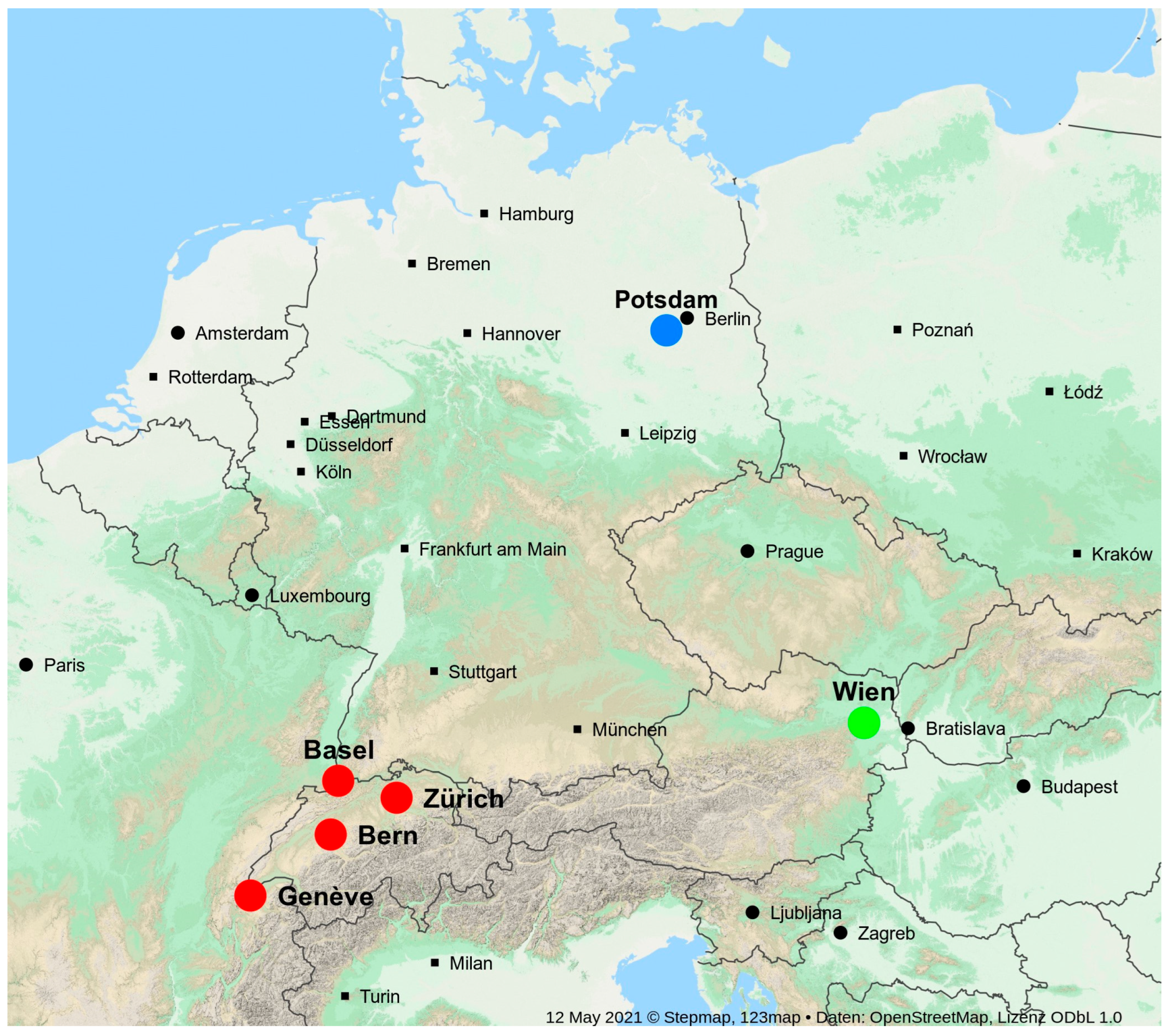
Figure 2.
Sunshine duration (SSD) in percent for summer half-year (April-September), 5y-averages, 1915-2022. 100% = average 1915-2022 for each station.
Figure 2.
Sunshine duration (SSD) in percent for summer half-year (April-September), 5y-averages, 1915-2022. 100% = average 1915-2022 for each station.
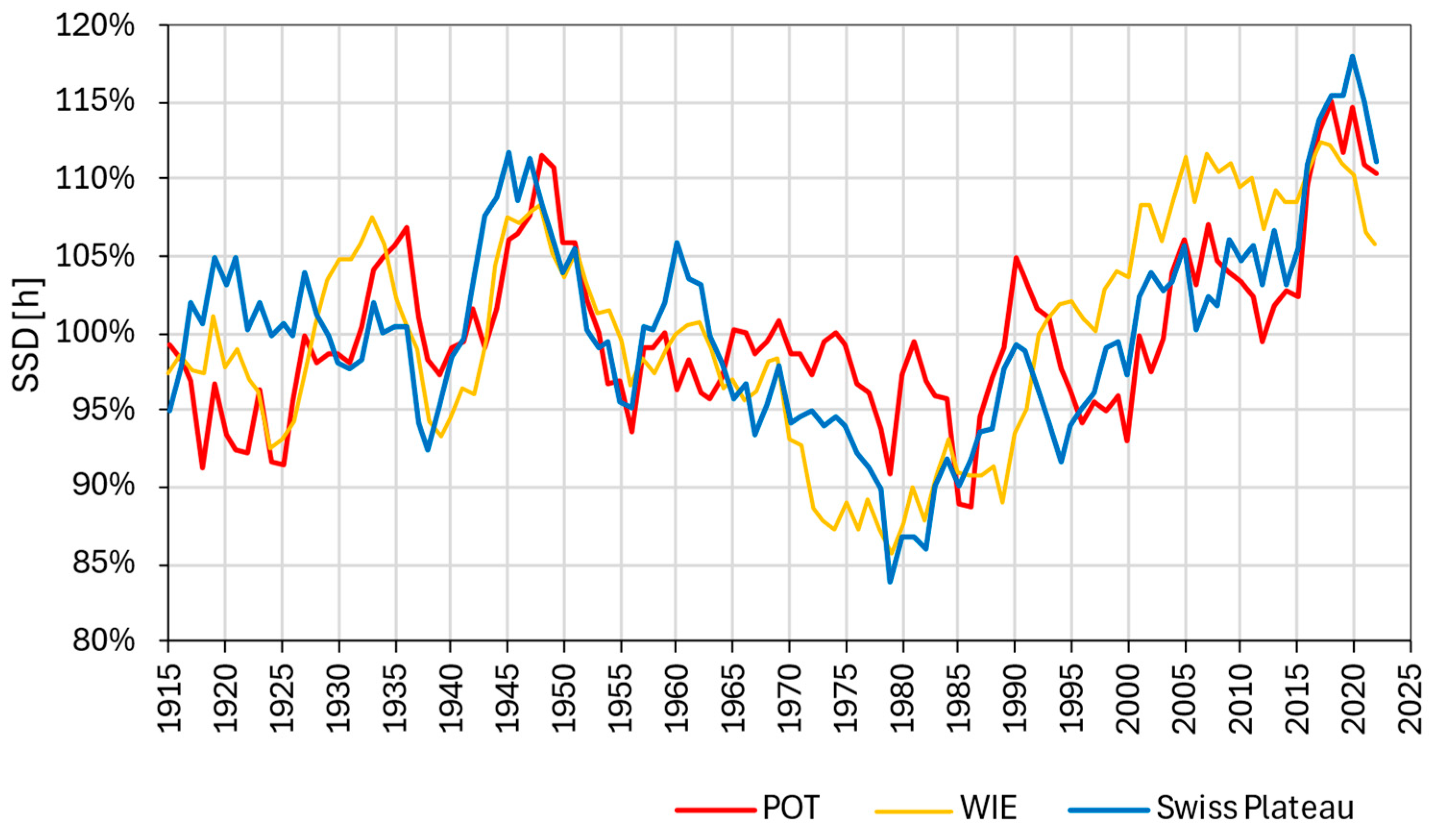
Figure 3.
Sunshine duration (SSD) in total hours, global radiation (GR) and cloudiness measured at Potsdam (D) for year, summer half-year (April-September) and summer (June-August), 5y-averages, 1895-2022.
Figure 3.
Sunshine duration (SSD) in total hours, global radiation (GR) and cloudiness measured at Potsdam (D) for year, summer half-year (April-September) and summer (June-August), 5y-averages, 1895-2022.
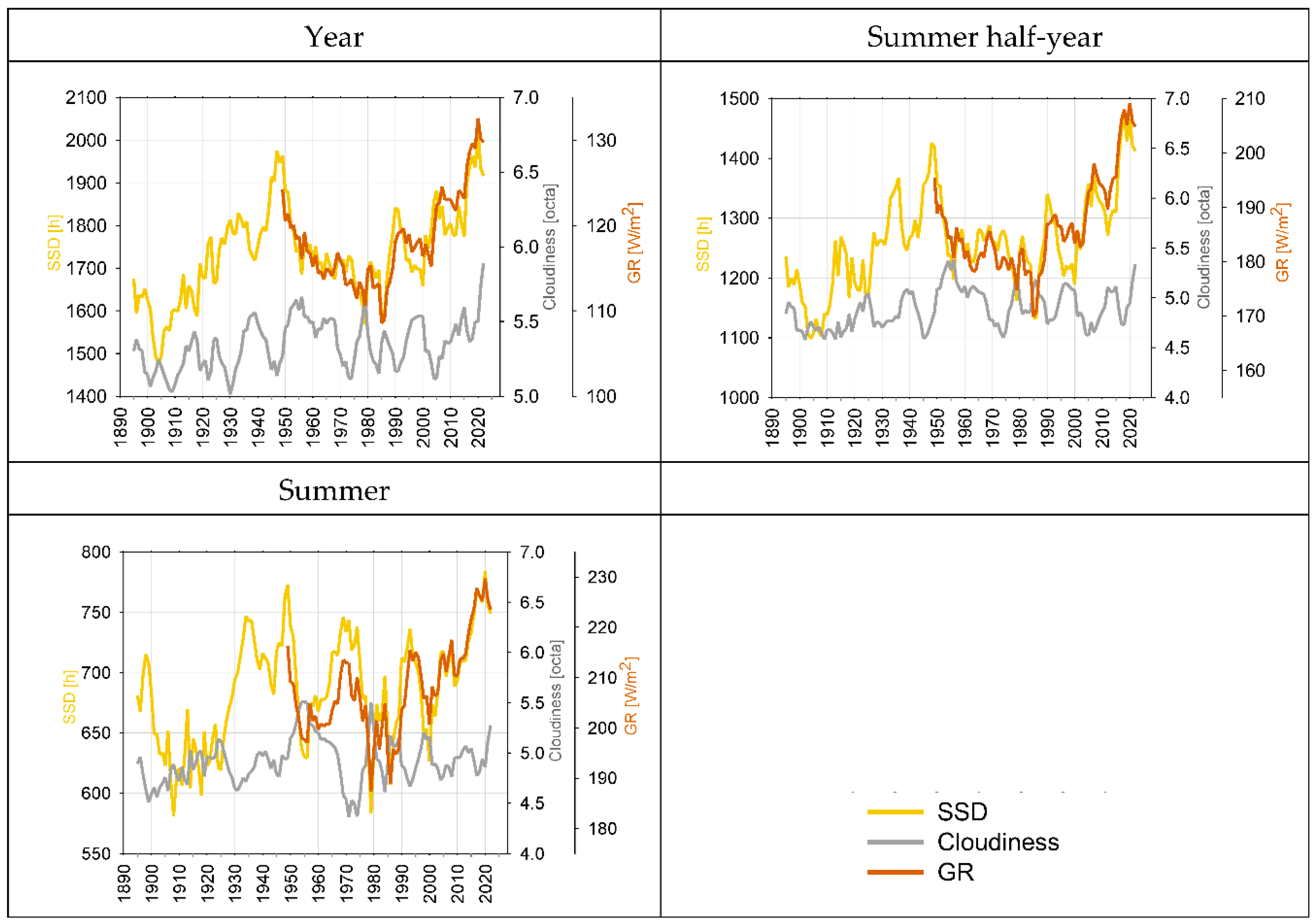
Figure 4.
Direct solar radiation DSR, measured at Potsdam, 5y-averages for summer half-year (April to September), 1947-2024. Left axis: DSR for cloud-free situations (cloudiness <= 2 octas; blue line). Right axis: DSR for cloudiness of 4-6 octas (orange line).
Figure 4.
Direct solar radiation DSR, measured at Potsdam, 5y-averages for summer half-year (April to September), 1947-2024. Left axis: DSR for cloud-free situations (cloudiness <= 2 octas; blue line). Right axis: DSR for cloudiness of 4-6 octas (orange line).
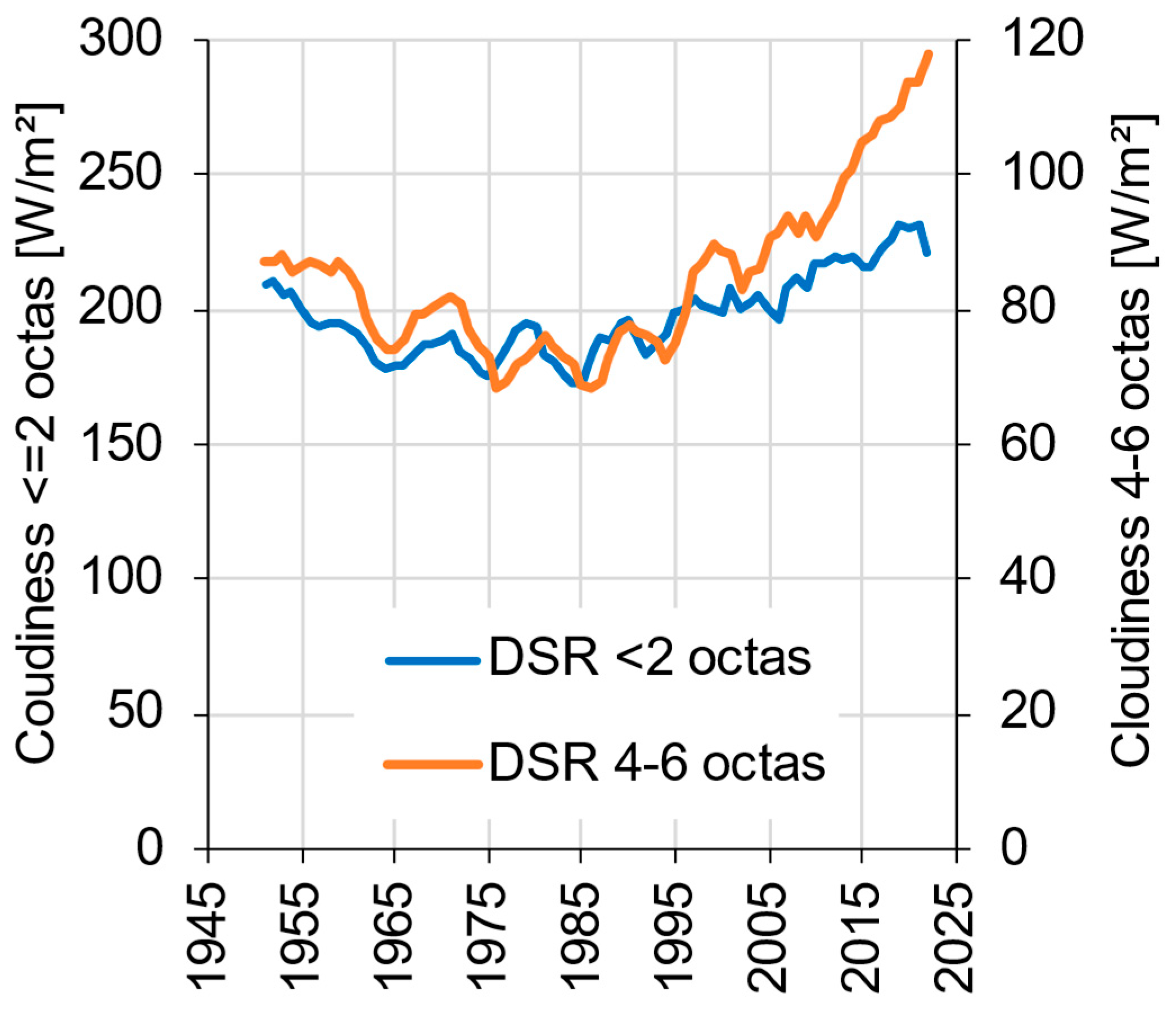
Figure 5.
Annual means of CO2 air concentration, 1895-2024. Measurements at Mauna Loa 1958-2024. Estimation for 1895-1958. y: approximation (s. equation) by regression for the whole period 1895-2024, starting with 279 ppb for 1895 (x = year-1895). Global mean (calculated by Carbon Cycle and Greenhouse Gases group), 1979-2023. Data (from the measurements at Mauna Loa and the global mean) provided by Carbon Cycle and Greenhouse Gases group, 325 Broadway R/GML, Boulder, CO 80305 (https://gml.noaa.gov/ccgg/).
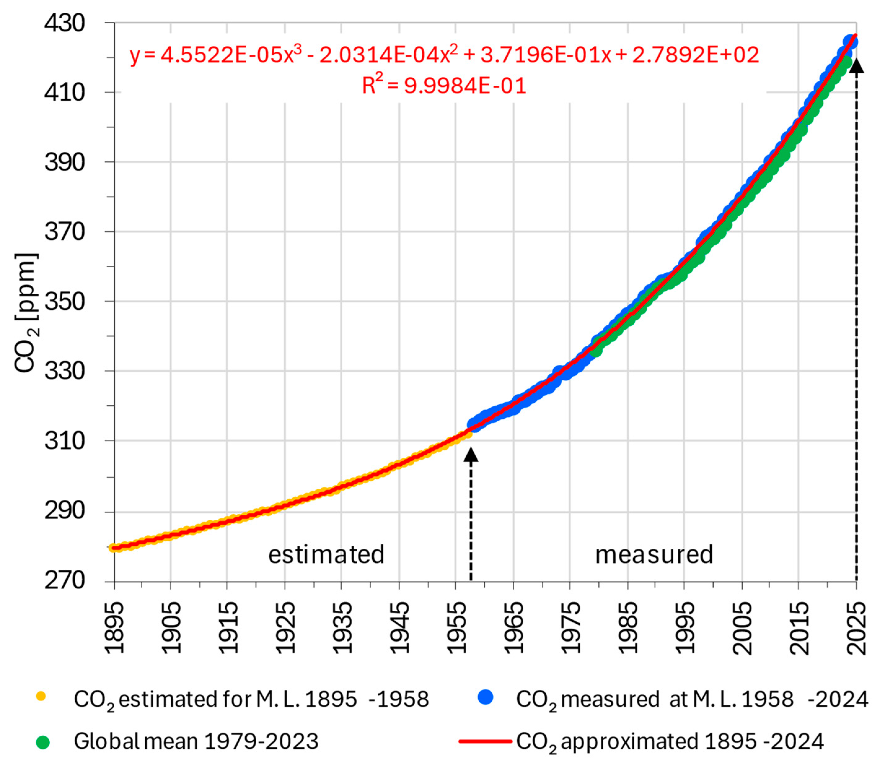
Figure 6.
Measured and model estimated temperature for summer (June-August), summer half-year (April to September) and entire year at Swiss Plateau, Potsdam and Wien, 1915-2022, 5-year averages.
Figure 6.
Measured and model estimated temperature for summer (June-August), summer half-year (April to September) and entire year at Swiss Plateau, Potsdam and Wien, 1915-2022, 5-year averages.
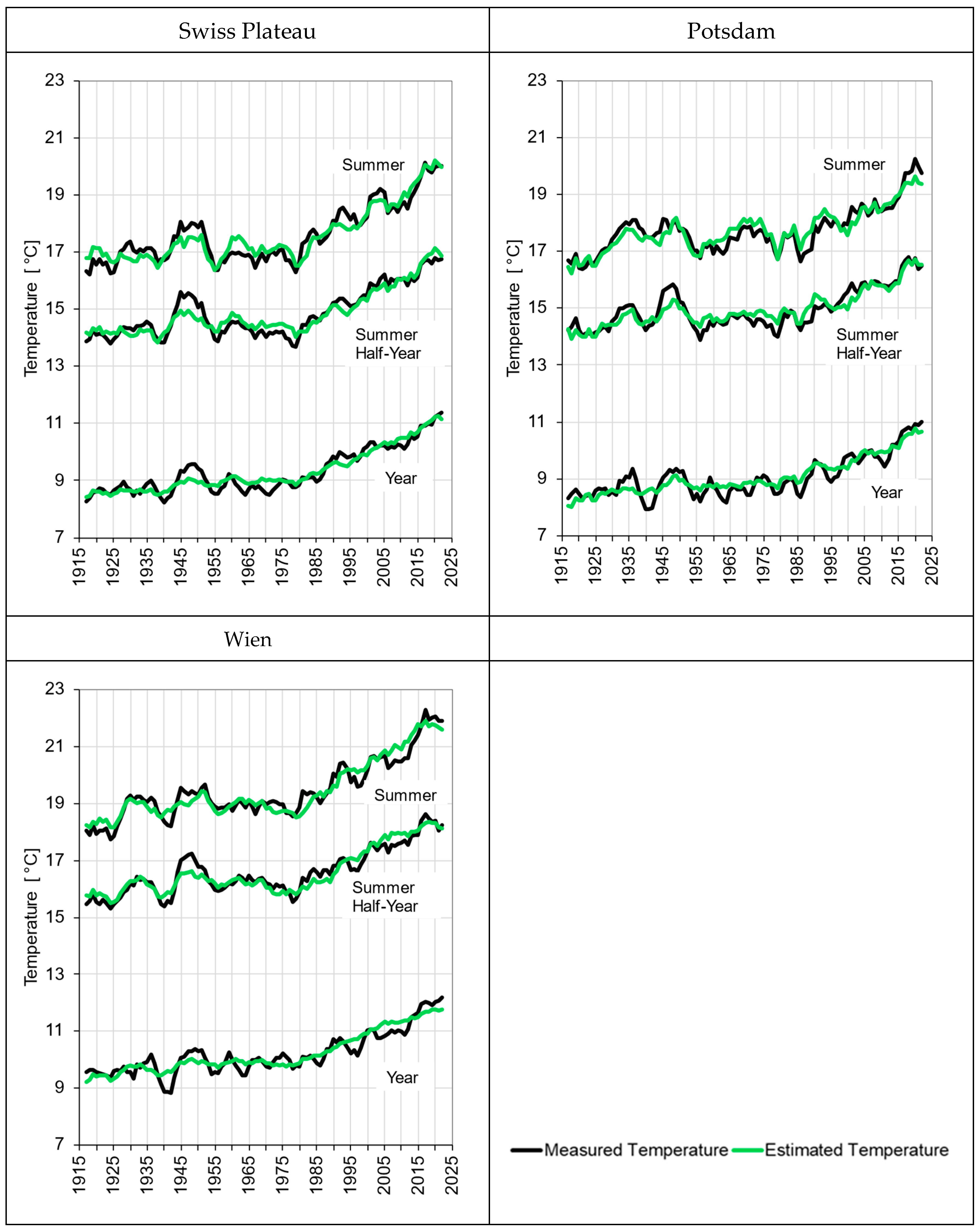
Figure 7.
Development of CO2 concentration, the accumulated fossil CO2 emissions and the emissions remaining in the atmosphere for a lifetime of 58 years for the period 1960-2023. Yearly fossil CO2 emissions worldwide since 1960 were evaluated by the Global Carbon Project GCP; CO2 air concentration represented by the Mauna Loa measurements since 1958, extrapolated backwards until 1895.
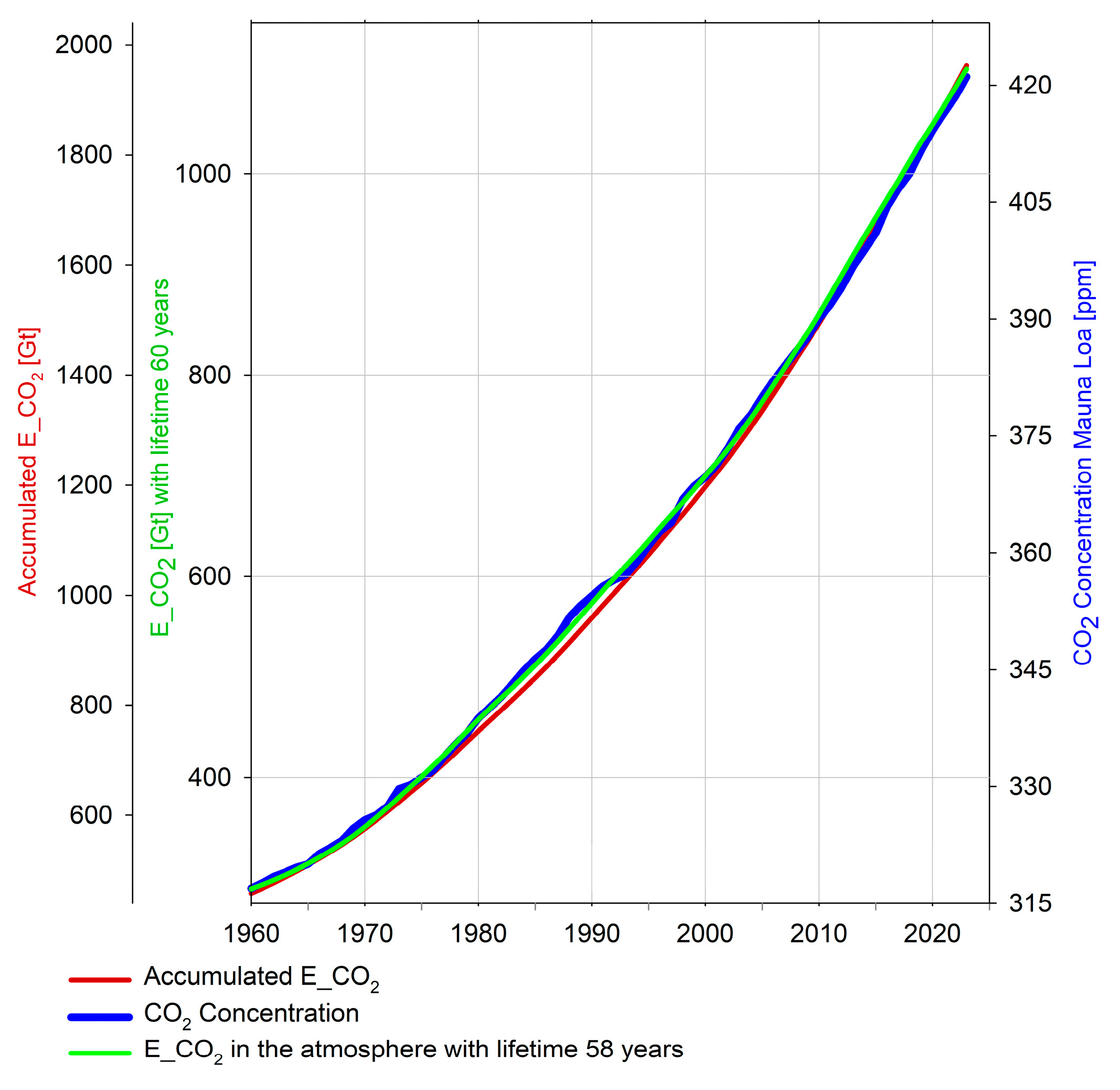
Figure 8.
Yearly fossil CO2 emissions worldwide in dependence on accumulated fossil CO2 emissions, 1960-2023. Yearly fossil CO2 emissions worldwide were evaluated by the Global Carbon Project GCP.
Figure 8.
Yearly fossil CO2 emissions worldwide in dependence on accumulated fossil CO2 emissions, 1960-2023. Yearly fossil CO2 emissions worldwide were evaluated by the Global Carbon Project GCP.
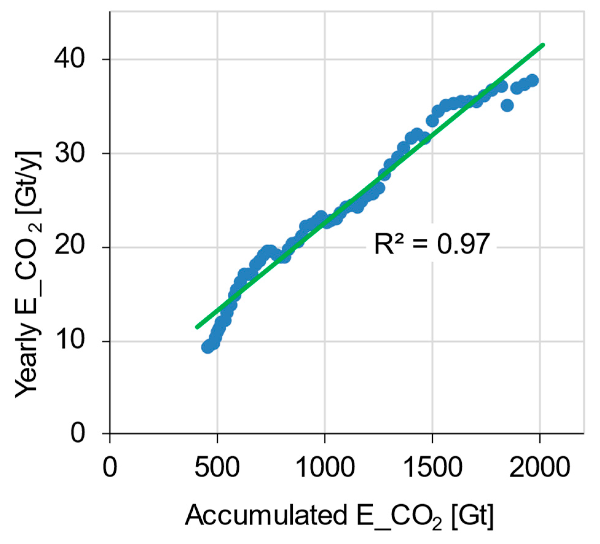

Table 1.
Names and coordinates of the measuring stations used in this study. Data was used for this study from 1915 until 2024.
Table 1.
Names and coordinates of the measuring stations used in this study. Data was used for this study from 1915 until 2024.
| Name of station | Abbr. | Longitude | Latitude | Altitude |
| [deg] | [deg] | [m a.s.l.] | ||
| Basel / Binningen | BAS | 7.583 | 47.533 | 316 |
| Bern / Zollikofen | BER | 7.467 | 46.983 | 553 |
| Genève / Cointrin | GVE | 6.128 | 46.248 | 411 |
| Zürich / Fluntern | ZRH | 8.567 | 47.383 | 556 |
| Potsdam | POT | 13.060 | 52.380 | 81 |
| Wien Hohe Warte | WIE | 16.356 | 48.249 | 198 |
Table 2.
Coefficients for SSD and CO2 from the regression model. Standard error of the estimated temperatures for yearly values and for 5-year averages. Summer half-year: April to September; summer: June-August.
Table 2.
Coefficients for SSD and CO2 from the regression model. Standard error of the estimated temperatures for yearly values and for 5-year averages. Summer half-year: April to September; summer: June-August.
| Coeff(SSD) | Coeff(CO2) | Std Error | Std Error | |
| [°C/(h/month)] | [°C/ppm] | [°C] | 5y-av. [°C] | |
| Year | 0.023 | 0.015 | 0.60 | 0.27 |
| Summer half-year | 0.026 | 0.014 | 0.52 | 0.27 |
| Summer | 0.027 | 0.019 | 0.59 | 0.31 |
Table 3.
Temperature increase D TT from 1915-2024 due to SSD and CO2 according to the regression model; relative shares of the total increase D TT(total). Summer half-year: April to September; summer: June-August.
Table 3.
Temperature increase D TT from 1915-2024 due to SSD and CO2 according to the regression model; relative shares of the total increase D TT(total). Summer half-year: April to September; summer: June-August.
| D TT(SSD) | D TT(CO2) | D TT(total) | D TT(SSD) | D TT(CO2) | |
| [°C] | [°C] | [°C] | rel. | rel. | |
| Year | 0.53 | 1.90 | 2.43 | 22% | 78% |
| Summer half-year | 0.76 | 1.76 | 2.52 | 30% | 70% |
| Summer | 0.85 | 2.30 | 3.14 | 28% | 72% |
Disclaimer/Publisher’s Note: The statements, opinions and data contained in all publications are solely those of the individual author(s) and contributor(s) and not of MDPI and/or the editor(s). MDPI and/or the editor(s) disclaim responsibility for any injury to people or property resulting from any ideas, methods, instructions or products referred to in the content. |
© 2025 by the authors. Licensee MDPI, Basel, Switzerland. This article is an open access article distributed under the terms and conditions of the Creative Commons Attribution (CC BY) license (http://creativecommons.org/licenses/by/4.0/).
Copyright: This open access article is published under a Creative Commons CC BY 4.0 license, which permit the free download, distribution, and reuse, provided that the author and preprint are cited in any reuse.


