
Submitted:
30 October 2025
Posted:
03 November 2025
You are already at the latest version
Abstract
Accurate 3D reconstructions of AEC structures using UAV photogrammetry are often hindered by occlusions, excessive image overlaps, or insufficient coverage, leading to inefficient flight paths and extended mission durations. This work presents a BIM-aware, autonomous UAS (Unmanned Aerial System) trajectory generation framework wherein a compact, geometrically valid viewpoint network is first derived as a foundation for path planning. The network is optimized via Integer Linear Pro-gramming (ILP) to ensure coverage of IFC-modeled components while penalizing poor stereo geometry, GSD, and triangulation uncertainty. The resulting minimal network is then sequenced into a global path using a Traveling Salesman Problem (TSP) solver and partitioned into battery-feasible epochs for operation on active construction sites. Evaluated on two synthetic and one real-world case study, the method produces au-tonomous UAV trajectories that are 31–63% more compact in camera usage, 17–35% shorter in path length, and 28–50% faster in execution time, without compromising coverage or reconstruction quality. The proposed integration of BIM modeling, ILP op-timization, TSP sequencing, and endurance-aware partitioning enables the framework for digital-twin updates and QA/QC monitoring. Accordingly, offering a unified, ge-ometry-adaptive solution for autonomous UAV inspection and remote sensing.
Keywords:
BIM‐aware planning
; camera network optimization
; UAV photogrammetry
; autonomous trajectory planning
; digital construction
1. Introduction
Accurate 3D reconstruction of complex infrastructure remains a challenge in UAV photogrammetry, particularly in the context of digital construction and autonomous inspection, where geospatial science and computer vision converge with the AEC industry. Structures such as bridges, towers, and industrial facilities introduce occlusions, height variations, and complex geometry that worsen visibility and flight planning challenges in UAV photogrammetry. Conventional approaches (e.g., grid or double-grid patterns) often disregard object-specific visibility constraints and generate redundant imagery, suboptimal reconstruction quality, and extended mission durations.
To address these limitations, this work proposes a BIM-aware framework for autonomous UAV trajectory planning and inspection, wherein a minimal camera network is used to generate efficient and feasible flight paths. At the core of the framework is a formal Integer Linear Programming (ILP) formulation [1] that selects the minimal subset of candidate camera poses satisfying strict coverage constraints while minimizing penalties related to stereo geometry (B/H), ground sampling distance (GSD), and 3D triangulation uncertainty. The selected camera positions are then sequenced using a Traveling Salesman Problem (TSP) [2] solver to generate an efficient UAV trajectory that is collision-checked against the BIM-derived voxel model. To ensure real-world feasibility, the optimized TSP trajectory is automatically partitioned into battery-constrained epochs, each fitting within a single UAV flight cycle, thereby enabling execution within standard endurance limits.
Using Building Information Models (BIM), dense candidate views are simulated over known geometry prior to flight. Since BIM/IFC models are central to digital construction workflows, this integration supports QA/QC processes, progress monitoring, as-built versus as-designed verification, and facilitates digital twin updates. The pipeline computes coverage-aware, geometry-compliant paths entirely offline, without relying on online SLAM [3,4] or onboard mapping for planning. Preplanned missions can be executed using standard navigation and localization methods such as GNSS, RTK, or visual–inertial odometry.
Unlike uniform or heuristic flight plans, the proposed framework generates autonomous, scene-adaptive trajectories derived directly from the optimized camera network. This coupling of ILP-based camera selection with TSP-based sequencing represents a key contribution, ensuring that UAV paths conform to the geometry and occlusion structure of each site. Crucially, the minimal camera network is not an end goal but rather a foundation for deriving efficient, flight-feasible trajectories that advance autonomous UAV inspection capabilities in infrastructure monitoring.
The framework is evaluated across three representative AEC scenarios: a steel truss bridge, a thermal power plant, and a real-world indoor construction site, demonstrating that compact, geometry-aware networks lead to significant reductions in camera usage and mission time, with only minor trade-offs in reconstruction quality.
This paper’s contributions are as follows:
- A formal ILP formulation for geometry-aware viewpoint network selection, ensuring that IFC-modeled components (e.g., columns, facades, structural elements) receive sufficient coverage while balancing photogrammetric quality terms (B/H, GSD, triangulation uncertainty). This provides a foundation for reliable as-built vs. as-designed verification.
- A BIM-driven pipeline for preflight trajectory planning, where dense visibility simulations over BIM/IFC geometry generate candidate views. This will ensure that UAV inspections also maintain the digital construction workflow while providing interoperability with existing project models and management systems.
- An adaptive trajectory planning method that sequences the optimized viewpoint networks into efficient, structure-aware UAV paths that implement TSP routing and partition the paths into battery-feasible epochs. This means that the planned missions can be made practical on active construction, while also enabling the delivery of auditable, repeatable inspection data that directly supports QA/QC, progress monitoring, and updates for the digital twins.
2. Related Work
Early UAV photogrammetry missions commonly relied on heuristic flight patterns such as grid or double-grid nadir surveys and façade sweeps [5,6]. While simple to implement, these methods generate redundant imagery and often suffer from poor stereo geometry and extended mission durations. Later, Xu, Wu [7] integrated “skeletal camera networks” into Structure-from-Motion (SfM) pipelines to improve reconstruction efficiency by pruning redundant connections between viewpoints; however, this approach may reduce angular diversity, remove useful redundancies for robustness, and does not explicitly optimize photogrammetric quality metrics.
Subsequent work on camera network optimization applied sequential filtering [8,9] or set-cover/submodular formulations [10,11]. These methods provided formal optimization potential but were often computationally heavy and lacked explicit enforcement of photogrammetric metrics such as base-to-height ratio (B/H), ground sampling distance (GSD), or triangulation accuracy.
In parallel, next-best-view (NBV) and exploration-based planners [12,13,14] addressed unknown or partially known environments by iteratively selecting new viewpoints during flight. While highly adaptive, they provide no global coverage guarantees and may converge to a local minimum, which limits their reliability for safety-critical inspection of known structures.
More recent approaches leverage digital twin or model-driven planning [15,16,17,18], where candidate viewpoints are informed by pre-existing models. Other works have directly coupled UAV inspection with BIM/digital twin workflows for QA/QC and progress monitoring [17,19,20]. While these works show the potential of model-guided inspection, they typically focus on coverage or image utility without integrating rigorous photogrammetric constraints or linking directly to IFC-based BIM workflows.
In contrast, our work combines global ILP-based camera network optimization with TSP-based trajectory planning, directly tied to BIM/IFC geometry. This ensures per-component coverage, photogrammetric quality, and mission feasibility, bridging the gap between minimal network design and practical UAV inspection in digital construction contexts.
To synthesize the discussion, Table 1 contrasts the main categories of UAV viewpoint and trajectory planning methods. Existing approaches range from heuristic or sequential filtering strategies to more formal submodular and NBV formulations, and more recently, digital-twin–guided planning. However, most either (i) focus on coverage without enforcing photogrammetric constraints, or (ii) treat viewpoint selection and routing as separate problems, without guaranteeing globally optimized and execution-feasible paths. In contrast, our framework uniquely combines ILP-based camera network optimization with TSP-based sequencing, directly tied to BIM/IFC geometry to ensure per-component coverage in digital construction workflows.
Positioning the Present Work
As summarized in Table 1, existing methods either rely on heuristic filtering or treat viewpoint selection and trajectory planning as separate problems, often without enforcing photogrammetric quality constraints. The proposed framework addresses these gaps by formulating viewpoint selection as a global ILP optimization over BIM-derived candidates, ensuring strict coverage of IFC components while preserving key photogrammetric quality measures. Crucially, the minimal network is not treated as an end in itself but as the foundation for trajectory generation: a TSP-based solver sequences the selected viewpoints into geometry-adaptive UAV paths that conform to scene complexity and are automatically partitioned into battery-constrained flight missions. To the best of our knowledge, this is the first framework to integrate global camera network optimization with trajectory planning in a BIM-aware pipeline. This coupling ensures operational efficiency and reconstruction fidelity while enabling autonomous UAV inspections to feed directly into QA/QC, progress monitoring, and digital twin updates in large-scale AEC and remote sensing contexts.
3. Methodology
This section presents the complete pipeline for autonomous UAV trajectory planning, integrated with BIM-aware, ILP-based camera network optimization. The proposed approach comprises three interconnected steps: (1) BIM-based scene preparation and visibility simulation, (2) camera network optimization via ILP, and (3) trajectory generation based on a Traveling Salesman Problem formulation. A summary of the proposed approach, illustrating the entire process, is provided in Figure 1. Moreover, the pipeline is designed to operate directly on IFC-based BIM models, ensuring interoperability with construction information systems and enabling inspection results to be integrated into digital twin environments.
3.1. BIM-Based Scene Preparation
The workflow begins with a high-resolution BIM of the target structure, provided in either mesh or IFC format. If the BIM model is not already in 3D mesh format, it is first converted, and a dense point cloud is sampled from its surfaces to simulate the as-designed geometry. Subsequently, visibility analysis is performed between the 3D points and a dense set of candidate camera poses. Candidate camera viewpoints are generated around the structure using standard photogrammetric patterns (e.g., double-grid, circular bands, and oblique views). Each candidate pose includes a 6-DOF position and orientation, and its visibility to scene points is evaluated via ray casting to construct a binary visibility matrix. This matrix encodes whether camera i observes point j and serves as the basis for camera selection. Because candidate viewpoints are tied to specific BIM/IFC elements (e.g., facades, columns, beams), coverage can later be evaluated per component, thereby supporting QA/QC and monitoring progress within autonomous digital construction workflows. This preprocessing step is essential for enabling offline mission planning, but does not represent the core contribution of this work.
3.2. ILP-Based Camera Network Optimization
The central contribution of this paper is an ILP formulation (Appendix A1) that selects a minimal yet photogrammetrically valid subset of candidate cameras. Each candidate's camera is associated with a binary decision variable , indicating whether it is selected.
Given candidate camera poses and 3D scene points, the optimization problem selects the smallest camera subset that ensures:
- Every scene point is observed by at least cameras (robust reconstruction)
- Favorable stereo geometry with optimal base-to-height (B/H) ratios
- Ground sampling distance (GSD) within acceptable thresholds
- Minimal 3D intersection uncertainty across selected views
- Overall sparsity for computational efficiency and mission autonomy.
The complete ILP formulation is explained as follows:
Each candidate camera is associated with a binary decision variable (Eq. 1), where represents the decision variables represented as:
A visibility matrix (Eq. 2) establishes the visibility between each camera and each point through geometric intersection and field-of-view checks:
With , the optimization problem is formulated as (Eq. 3):
Subject to the coverage and binary constraints (Eq. 4-5):
As mentioned, is the minimum number of cameras required to observe each point (). While are user-defined weights that tune the influence of the penalty terms (Appendix A). For all experiments, fixed weights are selected as (0.10,0.10,0.25) respectively (Table A1), giving slightly higher emphasis to intersection-angle accuracy.
In summary, the ILP objective in Eq. (3) combines sparsity with photogrammetric penalties under the coverage constraint in Eq. (4) and binary selection in Eq. (5), with decision variables defined in Eq. (1) and visibility given by Eq. (2).
This formulation yields a globally optimal solution within the defined constraints and visibility model that satisfies coverage requirements while prioritizing geometric strength. The flexibility of the linear penalty terms allows users to prioritize either sparse coverage or higher geometric quality, depending on application requirements. Figure 2 illustrates the general workflow of ILP-based camera optimization.
The detailed computation of penalty matrices , , and is presented in Section 3.3.
For large candidate networks, the ILP optimization employs multi-scale strategies to ensure computational tractability (Appendix A.2). Default parameter values are summarized in Table A1.
3.3. Quality-Based Penalty Functions
The ILP formulation introduced in the previous Section 3.2 includes three key penalty matrices: , , and , which respectively represent stereo geometry quality, ground sampling distance, and 3D triangulation uncertainty. These penalty functions are designed to discourage camera-point configurations that may compromise the geometric accuracy or visual quality of the final reconstruction. In this section, we describe the computation and interpretation of each penalty function in detail.
Specifically, stereo geometry is quantified via the B/H ratio in Eq. (6) with the penalty in Eq. (7); distance-based resolution is captured by the GSD substitution in Eq. (8) with the penalty in Eq. (9); and triangulation uncertainty contributes through Eq. (10) to the ILP objective as shown in Eq. (3).
3.3.1. Base-to-Height Ratio Penalty
For each scene point and each pair of candidate cameras that can see the point , the base-to-height ratio is:
where is the coordinate of the camera is the coordinate of the point .
For each camera-point pair , the penalty is defined as:
Where is a penalty assigned to the camera for viewing point with ratio outside the optimal range . , represent the acceptable interval for the base-to-height ratio.
This penalty term penalizes camera-point pairs whose stereo geometry would be too short-baseline or too wide-baseline, thus promoting optimal photogrammetric geometry.
3.3.2. Ground Sampling Distance Penalty
To ensure that each 3D scene point is imaged at a sufficient spatial resolution, a penalty is introduced based on the GSD as a proxy for image sharpness and detail capture.
For each camera-point pair , the GSD is approximated as proportional to the Euclidean distance between the camera center and the point:
Where is the position of the camera , and is the coordinate of the scene point .
To discourage views taken from excessively far distances (which reduce resolution), a normalized penalty is applied to camera-point pairs whose imaging distances exceed an acceptable threshold. The GSD-based penalty is defined as:
Where is the maximum acceptable distance at which high-resolution capture is assumed to still be achievable (e.g., based on sensor specs or mission requirements). is the penalty assigned to the camera for viewing point from beyond where (.
This penalty term ensures that camera viewpoints with unfavorable imaging geometry due to distance are penalized in the ILP objective, thereby promoting viewpoints that capture scene points with higher spatial resolution.
3.3.3. 3D Reconstruction Uncertainty Penalty
In addition to penalizing poor stereo geometry (via B/H ratio) and resolution degradation (via GSD), the third penalty term addresses the 3D reconstruction uncertainty of each point based on the geometric strength of multi-view intersection. This penalty favors camera configurations that result in precise triangulation, thereby improving the overall metric accuracy of the reconstructed point cloud.
For a given 3D point visible from a set of cameras, we estimate its intersection uncertainty using least-square multi-view triangulation over subsets of visible cameras. The standard deviation of the estimated point coordinates is computed from the posterior covariance matrix and is used as an indicator of spatial accuracy.
Let be a penalty assigned to the camera viewing point , based on how much the camera contributes to the intersection error when reconstructing the point .
is the combined uncertainty from the 3D intersection at point , and is a user-defined penalty weight for reconstruction uncertainty.
For each visible camera-point pair, the inverse of this uncertainty is used as a penalty proxy (i.e., higher error → higher penalty):
Here, is a large constant penalizing a numerically unstable configuration. For practical purposes, the values of are normalized to the range [0, 1] across all pairs.
Accordingly, this penalty term in Eq. 3 is designed to encourage the selection of camera configurations that provide geometrically robust and accurate 3D intersections, especially in scenes with complex topologies or long camera baselines. When combined with the B/H and GSD penalties, the ILP optimization effectively balances coverage, resolution, and spatial accuracy.
3.4. Trajectory Planning
Once the minimal set of camera viewpoints is selected using the ILP model, the next step involves computing an efficient autonomous UAV flight trajectory that visits each viewpoint exactly once, while avoiding collisions and minimizing total travel distance. This path optimization problem is formulated as a Traveling Salesman Problem (TSP), in which each selected camera pose represents a node, and edges are weighted by a cost function that incorporates both Euclidean distance and optional visibility scores.
The trajectory planning pipeline consists of several key steps (Figure 3):
- Input Preparation: Load a dense 3D point cloud of the BIM and extract the candidate camera positions from the ILP-optimized network. Define a voxel size appropriate to the UAV’s operational resolution (e.g., 1 meter).
- Preprocessing: Create a voxel grid over the scene geometry using the point cloud and specified voxel size. Compute a visibility score for each camera position relative to the scene points.
- Cost Matrix Computation: Construct a cost matrix using pairwise Euclidean distances between camera positions. Incorporate visibility scores to slightly favor viewpoints with better scene coverage.
- TSP Optimization: Solve the TSP using a nearest-neighbor heuristic or an external solver to determine an initial camera visitation order. Check the resulting trajectory for structural collisions via ray-based sampling and voxel intersection tests.
- Trajectory Postprocessing: Smooth the collision-free waypoint sequence using spline interpolation. Parameterize the dynamic trajectory with user-defined velocity and acceleration limits to conform to UAV motion constraints. Interpolate orientation angles (yaw, pitch, roll) across trajectory segments to ensure continuous transitions.
- Flight Time Estimation: Compute the total UAV travel distance from the smoothed trajectory. Estimate the flight time by summing segment-wise travel durations and per-waypoint hovering times, adjusted for environmental disturbances (e.g., wind).
The optimization goal is defined in Eq. (11) as:
Subject to the constraints Eq. (12) that each waypoint is visited exactly once, and the path forms a closed or open tour depending on the UAV mission design:
Here, is the distance between the waypoints and , is a binary decision variable indicating a path segment.
- Battery-Constrained Partitioning: Since the optimized trajectory will likely extend beyond the max endurance of a single UAV flight (≈30 min), the final trajectory is automatically partitioned into multiple flight epochs. Each epoch consists of subsets of waypoints and parts of the trajectory that may be executed in one battery cycle, ensuring complete coverage of waypoints in consecutive flight epochs without violating operational limits. From a digital-construction perspective, although flight-time constraints define epochs, the resulting autonomous mission segments can still be associated with IFC components or construction zones that happen to fall within each flight. This mapping enables inspection data from successive epochs to be aligned with site logistics and phased work packages, supporting structured QA/QC and progress monitoring.
The duration of an epoch is modeled in Eq. (13) as the sum of flight time, hover time at waypoints, and a multiplicative wind factor:
where
= length of leg between successive waypoints,
= UAV flying speed,
= number of waypoints in the epoch,
= per-waypoint hover time (for image capture),
= wind factor (safety margin).
An epoch is feasible if , where is the battery endurance (e.g., 30 min). To add an operational safety margin, we define an effective cap in Eq. (14).
with a small reserve fraction (e.g., =0.1, i.e., 10%).
The full TSP-ordered trajectory is then partitioned greedily by starting from the first waypoint, and the algorithm accumulates flight and hover times until the running total exceeds . At that point, the epoch is closed, and a new epoch begins from the next waypoint. This process continues until all waypoints are assigned.
Formally, let be the TSP-ordered waypoints and the segment length for . Define cumulative time as follows Eq. (15):
Where is the total hover time up to Epoch is defined as such that and is the maximum under this condition. This ensures that each epoch corresponds to a physically executable UAV flight bounded by a single battery cycle, while the union of all epochs preserves the full optimized TSP path.
Finally, the full optimized trajectory, including interpolated positions and orientations, is exported for simulation or direct execution on a UAV. The result is a smooth, collision-free, dynamically feasible, and battery-constrained flight plan adapted to the scene geometry. This ensures that UAV inspections deliver structured, component-level data suitable for integration with digital-twin and construction management systems.
3.5. Flight Execution
The optimized camera poses are executed by a rotary-wing UAV through waypoint-based navigation. The UAV autonomously follows a GPS/RTK-referenced trajectory generated by the TSP solver, where each waypoint corresponds to an ILP-selected camera pose. Images are automatically captured when the UAV reaches a predefined proximity (e.g., 0.5 m) to each waypoint, based on onboard GNSS and inertial sensing.
To maintain navigation stability in GNSS-degraded environments (e.g., under bridges or near tall structures), the mission can be executed using visual–inertial odometry (VIO) or an RTK fallback mode. Prior to flight, the BIM model can be used to identify potential signal-degraded areas and inform adjustments to flight parameters (e.g., increasing waypoint spacing, reducing speed, or modifying sensor-fusion strategies). This pre-integration of BIM ensures that autonomous flight execution remains consistent with construction site constraints, including known occlusions and access restrictions.
Mission duration is estimated directly from the optimized trajectory using the same timing model and parameters as those employed in the battery-constrained partitioning stage (i.e., flight time along segments plus per-waypoint hovering, with an applied wind/safety factor). This ensures consistency between the execution-time estimate and the epoch boundaries used to guarantee battery feasibility, enabling fair comparison between the optimized and dense networks in Section 4.
After data acquisition, the geotagged images from the optimized camera network are processed offline to generate a dense 3D model. Using only ILP-selected images reduces computational cost and redundancy while maintaining completeness. The resulting point cloud is georeferenced using known extrinsics or BIM-based control, yielding an accurate digital twin suitable for inspection, change detection, and other AEC applications.
3.6. Performance Metrics and Evaluation
To quantitatively assess the effectiveness of the optimized camera network, three complementary metrics will be used, which consist of Coverage Adequacy, Redundancy Ratio, and Network Efficiency. Together, these metrics assess how well the framework supports autonomous UAV mission efficiency, reconstruction accuracy, and robustness. In a digital-construction context, they also indicate how well UAV inspection data can be linked to BIM/IFC elements in a repeatable and auditable manner, which is critical for QA/QC and progress monitoring.
After optimization, the selected camera network is assessed using:
- Coverage Adequacy
Coverage adequacy Eq. (16) measures the proportion of scene points that are observed by at least the required minimum number of cameras (). It is defined as:
where is the total number of scene points, indicates the visibility of a point from camera , and is the binary selection variable for the camera .
A value close to 1 indicates that almost all scene points satisfy the minimum coverage requirement, which is essential for robust and accurate 3D reconstruction. At the construction scale, this means that all targeted components (e.g., floors, facades, or structural members) are sufficiently imaged for later verification against BIM models.
- 2.
- Redundancy Ratio
The redundancy ratio Eq. (17) quantifies the degree of excess coverage beyond the required minimum, normalized by the total number of camera-point observations:
This metric captures the fraction of all redundant visibility relationships, i.e., representing coverage beyond the minimum required. A moderate redundancy can be desirable for increasing robustness against occlusion or failures, but excessive redundancy indicates inefficiency. In construction practice, balancing redundancy ensures that critical elements are not undersampled, while avoiding unnecessary flights that slow down inspection cycles.
- 3.
- Network Efficiency
Network efficiency Eq. (18) evaluates the relative reduction in camera usage compared to the initial candidate set:
where is the total number of candidate cameras and is the number of cameras selected in the optimized network. A higher value indicates a more compact and efficient solution with fewer cameras retained. For digital construction, this translates into reduced mission time, fewer battery swaps, and lower processing overhead, making UAV-based inspections more practical for integration into routine QA/QC and progress monitoring workflows.
4. Results
To evaluate the effectiveness of the proposed ILP-based camera network optimization, we conducted three experiments using two detailed synthetic 3D models: (1) a steel truss bridge and (2) an industrial facility, and 3) real-world data of indoor construction. For all experiments, the optimization was performed with a minimum coverage requirement of =4. Each scene was reconstructed using both a full dense camera network and a filtered subset obtained via our ILP formulation. The performance of each configuration was assessed in terms of trajectory length, flight duration, reconstruction accuracy, and camera network quality metrics.
For each experiment, we present side-by-side comparisons of UAV flight paths, 3D reconstructions, and quantitative indicators, including Coverage Adequacy, Redundancy Ratio, and Network Efficiency. The results demonstrate that ILP optimization reduces redundant views and overall mission complexity while preserving acceptable geometric reconstruction quality. These outcomes confirm the potential of autonomous UAV planning frameworks to improve the safety, efficiency, and precision of infrastructure inspection missions. The following sections describe the experimental setup and findings in detail.
4.1. First Experiment: Steel Bridge Model
The first experiment is applied to a simulated medium-span steel truss bridge, which is modeled in Blender [21] and represented through its BIM-derived structural elements. The bridge spans approximately 40 meters in length and comprises key BIM components such as IfcBeam (horizontal and inclined steel beams), IfcMember (cross-braced trusses), IfcPlate (deck and under-bridge panels), IfcRailing (guardrails), and IfcElementAssembly (connection joints). These entities collectively form the semantic backbone for digital twinning, allowing inspection results and photogrammetric data to be directly indexed to individual bridge components.
Image acquisition was simulated with an RGB camera mounted to a UAV flying at an average altitude of 12 meters. The sensor setup assumed a consumer-grade APS-C camera (22.3 × 14.9 mm, 4752 × 3168 pixels) with a 25 mm focal length. This sensor setup represents a typical UAV payload used in infrastructure inspection. To ensure BIM-aware coverage, the original mission was designed to capture all relevant bridge components from different angles, including:
- Longitudinal side strips of oblique views are aligned with the truss members, ensuring full coverage of chords, diagonals, and connection joints.
- Top-down nadir strips covering the deck surface, guardrails, and load-bearing slabs.
- Under-bridge parallel strips targeting beams, deck undersides, and cross-bracing elements.
- Circular end loops capturing perspective-rich obliques of the bridge portals and pier–superstructure connections.
This BIM-guided perspective selection reflects autonomous UAV inspection priorities in structural monitoring to ensure redundancy for load-bearing members, visibility of fatigue-prone joints, and coverage of the deck’s service surfaces. The initial dense network consisted of 1522 candidate camera viewpoints, from which the ILP optimization selected 567 cameras (≈ 62% reduction) while satisfying the coverage and photogrammetric quality constraints.
The photogrammetric reconstruction yields a high-fidelity mesh and point cloud, which serves as the basis for evaluating accuracy, image reduction, and reconstruction efficiency between the traditional dense network and the BIM-informed, ILP-optimized network. Figure 4 compares the original preplanned trajectory (left), which encompasses all candidate viewpoints, with the BIM-aware optimized trajectory (right), where ILP-based camera selection is followed by TSP-based sequencing. The results highlight how autonomous BIM-aware planning supports lean yet reliable UAV missions by directly linking inspection imagery to structural components, enabling integration with asset management systems and digital twin workflows.
The ILP optimization yielded a more compact camera set with minor accuracy trade-offs (Table 2).
The optimized TSP trajectory for the steel bridge experiment produced a total flight distance of 2203 m. At a cruise speed of 2 m/s, with 2 seconds of hover per waypoint and a 5% wind factor, the mission duration was estimated at 39 minutes 12 seconds, exceeding the endurance of a single battery.
To ensure feasibility, the trajectory was partitioned into two epochs under the 27-minute battery cap (Table 3). Epoch 1 covers most viewpoints with a longer travel distance, while Epoch 2 completes the remaining coverage within a short 11-minute flight.
Figure 5 shows the UAV trajectory for the bridge case before and after battery life constraint partitioning.
4.2. Second Experiment: Industrial Facility
The 3D object used in this experiment represents a realistic industrial-scale scenario, modeled to simulate a thermal power plant and provided in .obj format as a purely geometric mesh. Although the source model does not contain semantic BIM information, it is treated as a BIM representation for this experiment. This assumption allows UAV viewpoints to be associated with functional building components and mapped to corresponding IFC classes, enabling BIM-aware flight planning and digital twin integration. The structure comprises the following BIM-assumed elements:
- IfcCoolingTower: A large cylindrical structure with a concave profile, representative of real evaporative cooling systems.
- IfcChimney: A tall, reinforced exhaust stack acting as the primary vertical landmark, prioritized for structural health monitoring and UAV inspection.
- IfcBuilding / IfcBuildingStorey: Block-shaped units of varying heights representing operational and maintenance buildings, subdivided into walls (IfcWall), slabs (IfcSlab), and access elements (IfcDoor, IfcWindow).
- IfcDistributionElement: Extensive pipework, ducts, and scaffolding surrounding the cooling tower, introducing significant occlusion and accessibility challenges for UAV-based photogrammetry.
- IfcSlab / IfcSite: The rectangular base platform, encompassing access areas, rooftop annexes, and flat operational surfaces.
The initial UAV imaging network was designed to ensure coverage of these BIM components through complementary flight trajectories:
- -
- Circular or spiral passes around the cooling tower (IfcCoolingTower) and chimney (IfcChimney) to achieve dense, multi-angle coverage of these critical vertical structures.
- -
- Horizontal oblique strips around the rectangular building blocks (IfcBuilding) to capture facades and rooftop slabs.
- -
- Close-range passes along scaffolding and pipework (IfcDistributionElement), designed to mitigate occlusions and ensure redundancy in visually complex areas.
- -
- Low altitude sweeps over the base platform (IfcSlab / IfcSite) to capture rooftop annexes, access points, and flat operational surfaces.
- -
- Curvilinear transitions between circular trajectories to maintain smooth motion continuity.
This model is ideal for evaluating UAV flight planning strategies, especially around tall vertical structures and intricate facades. It enables realistic testing of spiral or orbital UAV trajectories, obstacle-aware navigation, and photogrammetric reconstruction performance in complex industrial scenes. The object was imported into Blender and used as the primary 3D scene for simulating UAV imaging, trajectory generation, and pose evaluation in a controlled environment. As in the first experiment, the simulation used a sensor (22.3 × 14.9 mm) with 4752 × 3168 pixels resolution and a 25 mm focal length to emulate a realistic UAV imaging setup. The initial dense network consisted of 1263 candidate camera viewpoints, from which the ILP optimization selected 606 cameras (≈ 52% reduction) while satisfying the coverage and photogrammetric quality constraints. The visual comparison of UAV trajectories and resulting reconstructions for the full dense network and the ILP-optimized network is shown in Figure 6.
Table 4 summarizes the reconstruction accuracy and network efficiency metrics for the second test scene. Similar to the first test, the ILP-optimized network yields a more compact camera set with minor accuracy trade-offs.
The optimized TSP trajectory for the industrial plant dataset produced a total of 606 waypoints. The estimated mission duration was well above a single UAV battery limit. To ensure feasible flight execution, the trajectory was partitioned into two epochs (Table 5). Epoch 1 consumed the full 27-minute cap, while Epoch 2 completed the remaining coverage in just under 9 minutes.
Figure 7 shows the UAV trajectory before and after battery life constraint partitioning.
4.3. Third Experiment: Real-World Indoor Construction Site
The third real-world UAV experiment was conducted at the ITC faculty building of the University of Twente in the Netherlands. The hall-type structure is roughly 220 m long and 50 m wide; during data capture (autumn 2021), only the concrete-and-steel frame was standing, so the main load-bearing columns were fully visible and accessible for sensing.
The UAV platform used is a DJI Phantom 4 Pro v2, equipped with a 1-inch CMOS, 20 MP RGB camera (84° FOV, 24 mm equivalent focal length, mechanical shutter: 8 – 1/2000 s; maximum flight time ≈ 30 min). In this experiment, the actual calibrated focal length was 10.26 mm with a pixel size of 2.4 (corresponding sensor size ≈ 13.2 × 8.8 mm). The flight mission was executed in September 2021 with a ground-sampling distance (GSD) of ≈ approximately 1.5 cm and 90% front/side overlap to ensure high photogrammetric redundancy. Retro-targets were fixed to several interior columns; their coordinates were surveyed and used as GCPs for photo alignment, producing a locally oriented model tied to the BIM coordinate frame.
The as-planned BIM model, supplied by the University, was delivered in IFC format and contains only structural members. To use the BIM for the initial flight planning, the model was imported into Autodesk Revit for querying. Structural columns filtered and exported as STL meshes [22]. Then, a uniform point sampling converted the meshes to a reference point cloud as shown in Figure 8. Ground-floor columns whose bases dipped below 0 m (foundation level) were removed to match the UAV data extent.
Only the structural columns from the BIM model were used in the ILP optimization. This choice was motivated by the inspection objective that the columns are the primary load-bearing elements of the hall structure and, therefore, critical for geometric documentation and monitoring. By restricting the candidate visibility simulation to column surfaces, the optimization focused on ensuring complete and high-quality coverage of these essential components, while avoiding unnecessary viewpoints on non-structural elements. This design choice illustrates how UAV planning can be tuned to construction priorities, focusing capture on critical load-bearing elements while reducing redundant data collection.
The initial dense network comprised 3,025 candidate camera viewpoints, from which the ILP optimization retained 2078 cameras (≈31% reduction) while meeting the coverage requirement and photogrammetric quality constraints. The visual comparison of UAV trajectories and resulting reconstructions for the full dense network and the ILP-optimized network is shown in Figure 9.
Table 6 summarizes the reconstruction accuracy and network efficiency metrics for the second test scene. Like the first test, the ILP-optimized network yields a more compact camera set with minor accuracy trade-offs.
Since the optimized UAV trajectory exceeded the maximum endurance of ≈30 minutes per battery, the TSP path was divided into four epochs that fit within one battery cycle (Figure 10). Each epoch, as shown in Table 7, contains a subset of waypoints, with flight time and distance tailored to remain below the 27-minute operational cap (including hovering and wind safety margin).
Although Epoch 3 covers the longest path length (914 m), its duration remains within the 27-minute cap because flight time is relatively short compared to the cumulative hover time at each waypoint, which dominates the mission duration.
This real-world validation demonstrates the framework’s readiness for practical deployment in infrastructure inspection and monitoring, supporting repeatable, safety-aware UAV operations in constrained environments.
5. Discussion
The results from all three experiments highlight the effectiveness of the proposed ILP-based camera network optimization in balancing data efficiency and reconstruction quality. Across bridge, industrial facility, and indoor construction site cases, the ILP approach consistently achieved substantial reductions in both average cameras per point and overall network size, ranging from approximately 31% to nearly 63% while maintaining high coverage adequacy and acceptable geometric accuracy. In all experiments, the TSP-generated trajectories were automatically partitioned into battery-constrained epochs, ensuring mission feasibility within UAV endurance limits. This partition preserved the efficiency gains of the ILP optimization while producing autonomous, executable flight plans. The method ensures that flight planning remains tightly coupled with BIM/IFC geometry, allowing inspection outputs to be indexed by structural component and seamlessly reused within digital construction and remote-sensing workflows.
5.1. Trade-Offs and Reconstruction Quality
As shown in Table 2, Table 3, Table 4, Table 5 and Table 6, the ILP optimization consistently reduced camera count and redundancy across all experiments, while maintaining high coverage adequacy and only marginally increasing reconstruction error. These deviations, which were at the millimeter level for the bridge and indoor site and at the centimeter level for the industrial facility, remain well within practical tolerances for UAV-based inspection. These results illustrate a deliberate trade-off: leaner image sets and shorter missions in exchange for a slight loss in accuracy, which is acceptable in most as-built verification and monitoring contexts where mission autonomy and operational efficiency are prioritized.
5.2. Mission Efficiency and Practical Value
The shorter UAV trajectories and reduced mission durations, shown in Figure 5, Figure 7 and Figure 10 (and Figure 6, Figure 8 and Figure 11 for battery-constrained partitioning), illustrate the operational benefits of ILP-based planning. For example, in the bridge experiment, the optimized trajectory reduced flight distance by over 790 meters and saved more than 40 minutes of mission time. In the industrial facility, flight time was reduced from 64 to 37 minutes, and in the indoor construction case, from 144 to 104 minutes. These reductions represent a significant improvement in safety, autonomy, and energy efficiency for UAV inspection.
To ensure feasibility, the optimized TSP trajectories were further partitioned into battery-constrained epochs, each fitting within a single UAV flight cycle (approximately 20 to 27 minutes). Across the three experiments, this resulted in two to four epochs per mission, providing complete coverage while respecting endurance limits. This automatic partitioning preserved the global efficiency of the ILP–TSP optimization and produced flight plans that were directly executable in practice.
The optimized camera networks also yielded cleaner TSP-based paths, minimized hover-and-capture actions, and reduced both energy consumption and mechanical wear. In construction contexts, this translated into fewer battery swaps, shorter on-site inspection windows, and reduced disruption to other site activities, making autonomous UAV-based inspections easier to integrate into daily project workflows. By incorporating photogrammetric quality metrics, such as B/H ratios, GSD, and triangulation uncertainty, as soft penalties in the ILP objective, the framework enforced both geometric soundness and resource-efficient planning.
5.3. Limitations
The current framework assumes an idealized execution environment and does not explicitly model environmental disturbances such as wind, GNSS signal loss, or temporary occlusions. These factors can affect the UAV’s ability to reach planned viewpoints or maintain correct camera orientation, particularly in outdoor settings. Therefore, further validation in complex real-world and GNSS-challenged environments is required to assess robustness under real-world conditions.
The method also assumes a uniform coverage requirement for all 3D points, which may not be suitable for applications where certain areas demand denser sampling due to structural criticality or inspection standards. A logical extension would be to incorporate IFC-based component weighting, ensuring that critical elements such as load-bearing columns, joints, or façades receive higher guaranteed coverage.
Collision checking is conducted using ray-based tests on a BIM-derived voxel model. Consequently, safety guarantees are model-relative and may not account for unmodeled obstacles or dynamic scene changes such as scaffolding, vehicles, or personnel. Operational safety thus still depends on on-site procedures and, when necessary, onboard sensing.
Additionally, operational logistics between battery-constrained epochs, such as takeoff and landing, battery replacements, waypoint reinitialization, RTK or communication relock, and crew repositioning, are not modeled. These factors impose non-negligible timing and safety constraints that can influence feasible epoch boundaries. Permissions for launch and landing, availability of safe staging areas, and coordination with other site activities also remain outside the current planning scope.
5.4. Behavior and Strengths of the ILP Optimization
The ILP formulation ensured globally optimal camera selection within minutes, even for networks with thousands of candidates. Unlike heuristic filtering, it guarantees per-point coverage while balancing photogrammetric quality penalties such as B/H, GSD, and triangulation uncertainty. By adjusting penalty weights, operators can flexibly prioritize either coverage density or geometric accuracy. This globally optimal and tunable optimization behavior contributes to the framework’s robustness across the three diverse test cases and demonstrates its suitability for autonomous, large-scale UAV inspection and monitoring tasks.
6. Conclusions
This study introduced a BIM-aware and autonomous UAV framework for optimal camera-network selection and trajectory planning in photogrammetric infrastructure inspection. By jointly optimizing camera placement with respect to coverage, stereo geometry, ground-sampling distance (GSD), and triangulation uncertainty, the method generates compact camera configurations that preserve high reconstruction quality. Integration with a TSP-based sequencing strategy enables efficient, collision-checked trajectories adapted to scene geometry and constrained by the BIM model. Because the entire pipeline is driven by BIM and IFC data, inspection outputs can be indexed to specific structural components, ensuring traceable coverage valuable for construction QA/QC and digital-twin workflows.
Evaluation across three distinct case studies, a simulated steel bridge, a simulated industrial facility, and a real-world indoor construction site, demonstrated substantial reductions in camera usage, ranging from 31 to 63 percent, along with significant mission time savings (up to 50 %). These benefits were achieved with only minor trade-offs in reconstruction accuracy. The approach was computationally efficient, adaptable to both synthetic and real environments, and directly executable in multi-flight missions through battery-constrained epoch partitioning. This capability enabled complete coverage of large or complex structures while maintaining feasibility within UAV endurance limits. The resulting gains translated into fewer images to process, fewer battery swaps, and leaner inspection missions, ultimately reducing operational overhead while maintaining the fidelity required for as-built verification.
Several directions exist for further development. These include validating performance in outdoor environments affected by wind, lighting variability, and GNSS degradation, and extending the system to support cooperative or multi-UAV planning for larger infrastructure. Future work should also explore component-weighted optimization for prioritizing critical structural elements, tighter integration with cloud-based digital-twin platforms, and automated links to progress-monitoring systems. With these enhancements, the framework can evolve into a fully autonomous, field-ready UAV inspection tool that bridges remote sensing, robotics, and digital construction—delivering pre-planned, auditable, and data-driven inspection outputs for QA/QC, maintenance, and infrastructure management.
Author Contributions
Conceptualization, B.A. and Y.H.K.; methodology, N.A.A., Z.N.J., B.A., and H.A.H.; software, N.A.A., B.A., and H.A.H.; validation, N.A.A., Z.N.J., and B.A.; analysis, N.A.A. and H.A.H.; resources, B.A.; data curation, H.A.H.; writing—original draft preparation, B.A.; writing—review and editing, N.A.A.; visualization, B.A., and N.A.A.; supervision, B.A.; All authors have read and agreed to the published version of the manuscript.
Funding
This research received no external funding.
Data Availability Statement
The data used in this study include two synthetic 3D models (a steel bridge and an industrial facility) and a real-world UAV dataset collected at the University of Twente construction site. Due to institutional and privacy restrictions, the real-world dataset is not publicly available. The synthetic models and corresponding simulation data are available from the corresponding author upon reasonable request.
Conflicts of Interest
The authors declare no conflicts of interest.
Appendix A
A.1. Integer Linear Programming Foundation
ILP is a subclass of mathematical optimization problems where the objective function and all constraints are linear. Still, the decision variables are restricted to integer values that are typically binary (0 or 1) for selection problems. A standard ILP problem for variables and constraints can be written as:
where:
vector of integer decision variables,
: cost coefficients,
matrices of inequality and equality constraints,
: right-hand side vectors of inequality and equality constraints,
the lower and upper bounds of (typically 0 and 1).
ILP is widely used in problems involving selection, allocation, and scheduling where discrete decisions must be made. Despite being NP-hard in general, modern solvers (e.g., branch-and-bound, cutting planes) can efficiently solve large ILP problems due to advances in integer programming techniques.
In this work, ILP is chosen to solve the camera network optimization problem because it allows us to:
enforce binary selection of cameras,
embed multiple constraints (e.g., point coverage),
and incorporate complex photogrammetric quality metrics in a unified linear framework.
This mathematical structure enables globally optimal selection of a minimal yet geometrically sound camera network, while remaining tractable for practical problem sizes using off-the-shelf ILP solvers. Worth mentioning that the ILP problem implemented and solved in this paper using MATLAB’s (R2024a) ‘intlinprog’ function from the Optimization Toolbox [23], which uses branch-and-bound and cutting plane algorithms to guarantee global optimality. No external solver (e.g., Gurobi or CPLEX) was required.
A.2. ILP Implementation Details
The ILP-based camera selection adapts its solving strategy to the size of the candidate network in order to balance computational efficiency with solution quality. While Figure 2 shows the overall framework, Figure A1 details the conditional solving paths:
- Small networks: solved directly by ILP.
- Medium networks: solved using an overlapping-cluster strategy.
- Large networks: solved using a hierarchical boundary-coherent strategy.
In all cases, the solver enforces coverage and photogrammetric constraints while incorporating penalties for GSD, base-to-height ratio, and triangulation accuracy. If the solver cannot reach feasibility within the given runtime or gap tolerance, the system activates a greedy or boundary-aware fallback to guarantee full coverage. The output always includes the selected cameras, the achieved objective value, and computation time, which are then passed to the results stage.
The optimization relies on a set of tunable thresholds that balance solver efficiency, photogrammetric quality, and robustness (Table A1). Coverage thresholds drive the ILP constraints, while penalty weights (B/H, GSD, triangulation) shape the objective. For extensive networks, a subset of parameters is automatically adjusted to ensure tractability within practical runtimes.
The final objective function combines four terms: (i) sparsity in the number of selected cameras, (ii) stereo geometry penalties discouraging poor B/H ratios, (iii) distance-based GSD penalties, and (iv) triangulation accuracy penalties. These are applied under two constraints: every 3D point must be observed by at least kmin cameras (Coverage Constraint), and each camera is either selected or not (Binary Constraint). Together, these ensure a compact yet geometrically sound network while allowing flexible trade-offs between efficiency and accuracy.
Figure A1.
Detailed workflow of the ILP-based camera network optimization, showing hierarchical, cluster, and direct solving paths with fallback strategies.
Figure A1.
Detailed workflow of the ILP-based camera network optimization, showing hierarchical, cluster, and direct solving paths with fallback strategies.
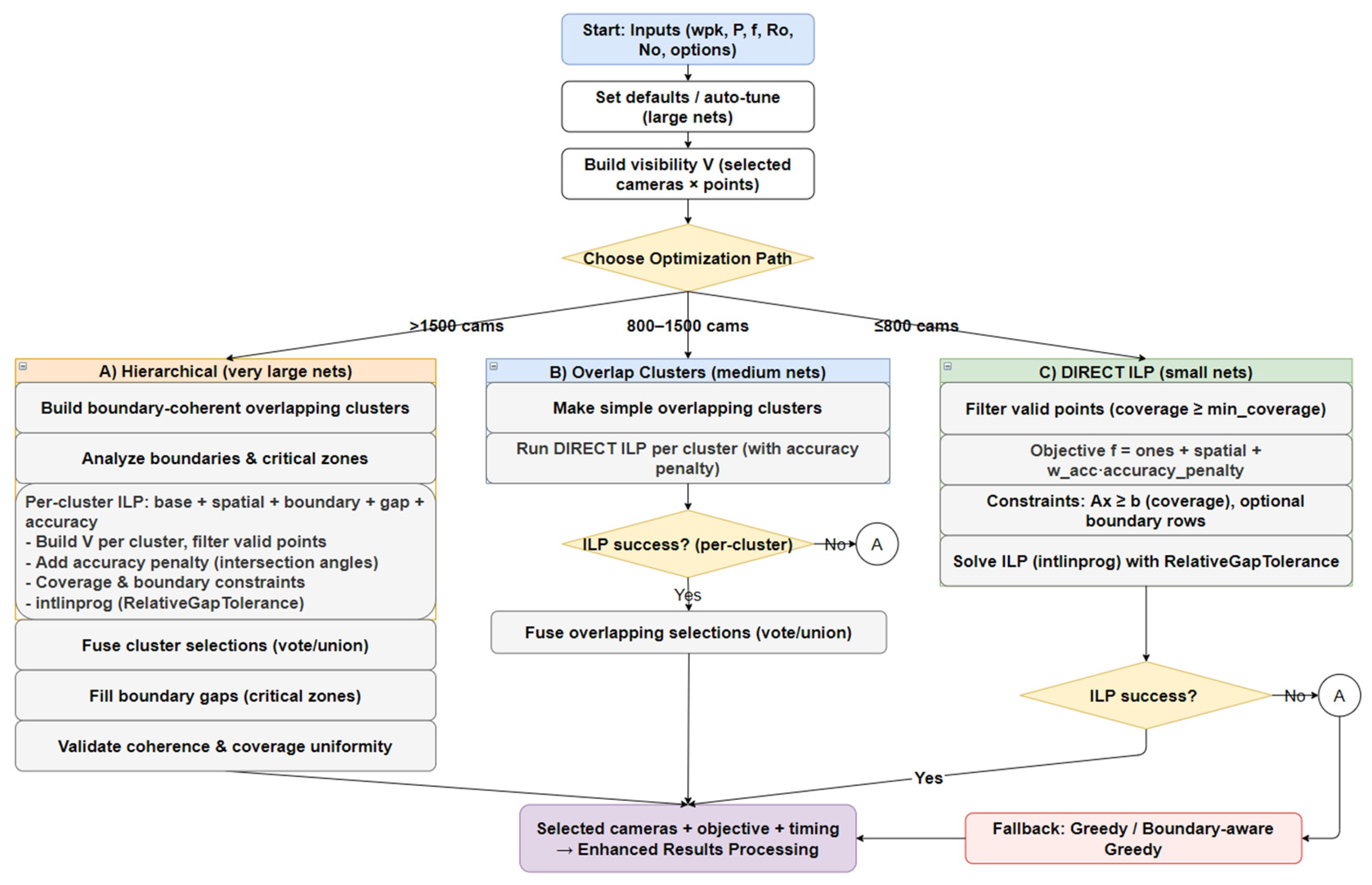

Table A1.
Optimization parameters used in the experiments.
| Category | Parameter | Default Value |
|---|---|---|
| Coverage / Solver | Minimum cameras required per 3D point | 3 |
| Maximum solver runtime | 600 s | |
| Early stop tolerance on MILP relative gap | 0.15 | |
| Photogrammetric Quality | Weight for the base-to-height ratio penalty | 0.1 |
| Weight for ground sampling distance penalty | 0.1 | |
| Weight for intersection-angle penalty | 0.25 | |
| Lower B/H bound | 0.2 | |
| Upper B/H bound | 0.6 | |
| Fraction of points sampled for angle computation | 0.2 | |
| Angles below the threshold are considered weak triangulation | 20° | |
| Above threshold, diminishing returns are assumed | 90° | |
| Robustness / Cleaning | Tolerated fraction of noisy or unstable points | 0.05 |
| Hierarchical / Boundary Coherence | Enable hierarchical optimization path for large networks | TRUE |
| Redundancy prefilter threshold | 0.8 | |
| Cluster overlap fraction | 0.2 | |
| Buffer zone for boundary coherence | 100 m | |
| Weight for boundary camera incentive | 0.25 | |
| Minimum required cameras in boundary zones | 3 | |
| Weight for gap-prevention heuristic | 0.3 |
References
- PAN, P.-Q., Integer Linear Programming (ILP), in Linear Programming Computation. 2014, Springer Berlin Heidelberg: Berlin, Heidelberg. p. 275-294.
- Zhang, C. and P. Sun. Heuristic Methods for Solving the Traveling Salesman Problem (TSP): A Comparative Study. in 2023 IEEE 34th Annual International Symposium on Personal, Indoor and Mobile Radio Communications (PIMRC). 2023. [CrossRef]
- Nava, Y. and P. Jensfelt, Visual-LiDAR SLAM with loop closure. 2018.
- Santos, J.M., D. Portugal, and R.P. Rocha. An evaluation of 2D SLAM techniques available in Robot Operating System. in 2013 IEEE International Symposium on Safety, Security, and Rescue Robotics (SSRR). 2013. [CrossRef]
- Nex, F. and F. Remondino, UAV for 3D mapping applications: a review. Applied Geomatics, 2014. 6(1): p. 1-15. [CrossRef]
- Colomina, I. and P. Molina, Unmanned aerial systems for photogrammetry and remote sensing: A review. ISPRS Journal of Photogrammetry and Remote Sensing, 2014. 92: p. 79-97. [CrossRef]
- Xu, Z., et al., Skeletal camera network embedded structure-from-motion for 3D scene reconstruction from UAV images. ISPRS Journal of Photogrammetry and Remote Sensing, 2016. 121: p. 113-127. [CrossRef]
- Alsadik, B., et al., Minimal Camera Networks for 3D Image Based Modeling of Cultural Heritage Objects. Sensors, 2014. 14(4): p. 5785-5804. [CrossRef]
- Alsadik, B., M. Gerke, and G. Vosselman, Automated camera network design for 3D modeling of cultural heritage objects. Journal of Cultural Heritage, 2013. 14(6): p. 515-526. [CrossRef]
- Kritter, J., et al., On the optimal placement of cameras for surveillance and the underlying set cover problem. Applied Soft Computing, 2019. 74: p. 133-153. [CrossRef]
- Roberts, M., et al., Submodular Trajectory Optimization for Aerial 3D Scanning. 2017 IEEE International Conference on Computer Vision (ICCV), 2017: p. 5334-5343.
- Lauri, M., et al., Multi-Sensor Next-Best-View Planning as Matroid-Constrained Submodular Maximization. IEEE Robotics and Automation Letters, 2020. 5(4): p. 5323-5330. [CrossRef]
- Bircher, A., et al., Receding Horizon "Next-Best-View" Planner for 3D Exploration. 2016 IEEE International Conference on Robotics and Automation (ICRA), 2016: p. 1462-1468. [CrossRef]
- Peng, C. and V. Isler, Adaptive View Planning for Aerial 3D Reconstruction. 2019 International Conference on Robotics and Automation (ICRA), 2018: p. 2981-2987. [CrossRef]
- Wang, L., et al., Digital-twin deep dynamic camera position optimisation for the V-STARS photogrammetry system based on 3D reconstruction. International Journal of Production Research, 2024. 62(11): p. 3932-3951. [CrossRef]
- Alizadehsalehi, S. and I. Yitmen, Digital twin-based progress monitoring management model through reality capture to extended reality technologies (DRX). Smart and Sustainable Built Environment, 2021. 12(1): p. 200-236. [CrossRef]
- Ojeda, J.M.P., et al., Estimation of the Physical Progress of Work Using UAV and BIM in Construction Projects. Civil Engineering Journal, 2024. [CrossRef]
- Zhang, S., W. Zhang, and C. Liu, MODEL-BASED MULTI-UAV PATH PLANNING FOR HIGH-QUALITY 3D RECONSTRUCTION OF BUILDINGS. Int. Arch. Photogramm. Remote Sens. Spatial Inf. Sci., 2023. XLVIII-1/W2-2023: p. 1923-1928. [CrossRef]
- Jacob-Loyola, N., et al., Unmanned Aerial Vehicles (UAVs) for Physical Progress Monitoring of Construction. Sensors (Basel, Switzerland), 2021. 21. [CrossRef]
- Salem, T., M. Dragomir, and E. Chatelet, Strategic Integration of Drone Technology and Digital Twins for Optimal Construction Project Management. Applied Sciences, 2024. 14(11): p. 4787. [CrossRef]
- Blender, Blender Foundation, in a 3D modelling and rendering package, S.B. Foundation, Editor. 2025: Amsterdam.
- Tsige, G.Z., et al., Automated Scan-vs-BIM Registration Using Columns Segmented by Deep Learning for Construction Progress Monitoring. Int. Arch. Photogramm. Remote Sens. Spatial Inf. Sci., 2025. XLVIII-G-2025: p. 1455-1462. [CrossRef]
- Inc., M., Mixed-integer linear programming (MILP). 2024, Mathworks Inc.: USA.
Figure 1.
BIM-based framework. The candidate viewpoints are simulated from IFC models, optimized with ILP, and sequenced into UAV trajectories via TSP and battery partitioning.
Figure 1.
BIM-based framework. The candidate viewpoints are simulated from IFC models, optimized with ILP, and sequenced into UAV trajectories via TSP and battery partitioning.
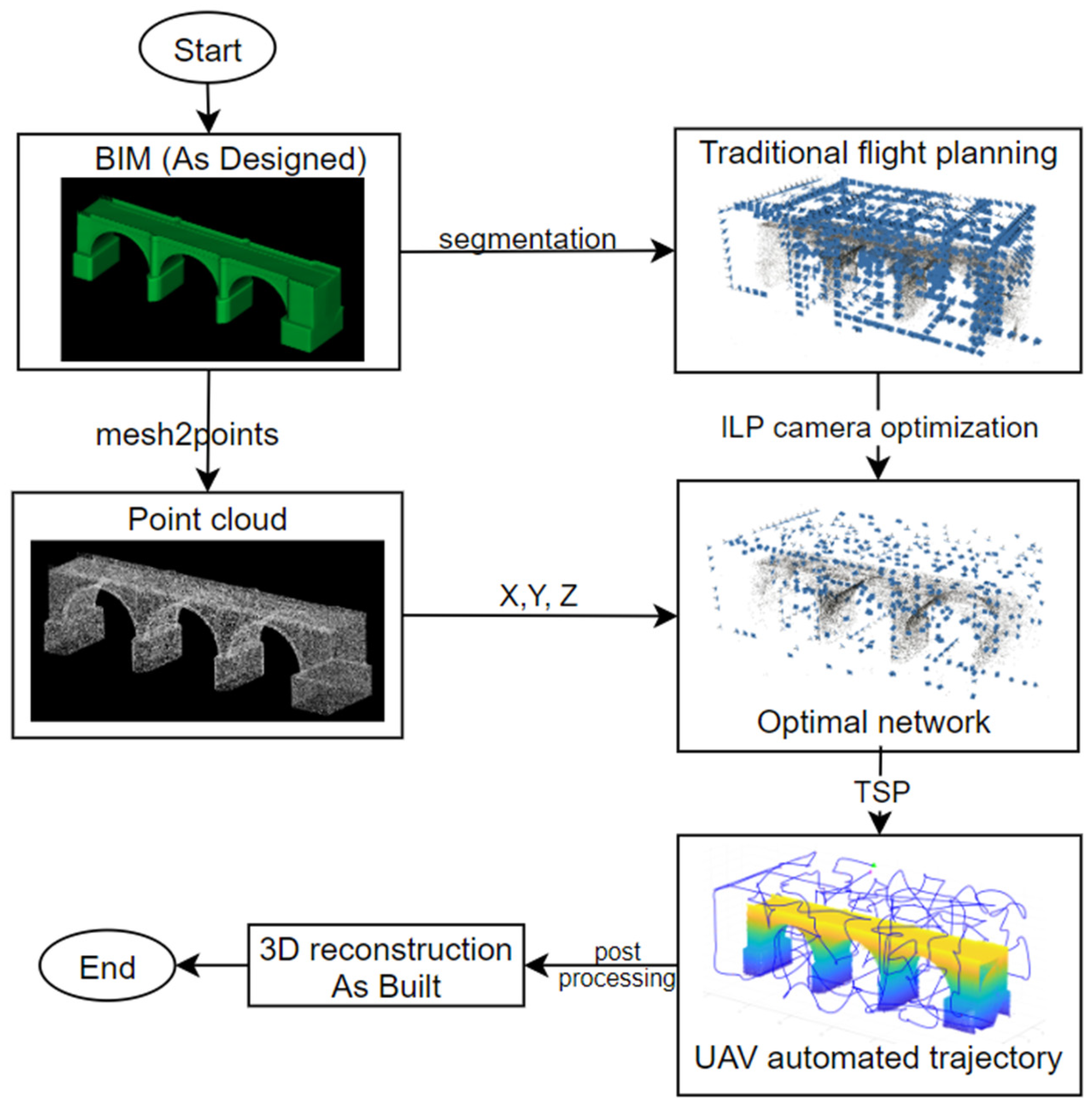
Figure 2.
Camera network optimization solution using Integer Linear Programming (ILP).
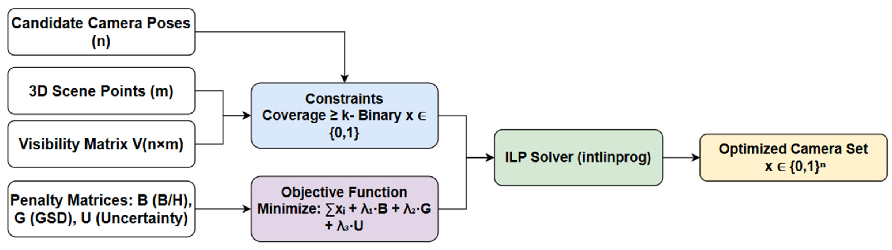
Figure 3.
Overview of the UAV trajectory planning pipeline using voxel grid analysis and TSP-based optimization.
Figure 3.
Overview of the UAV trajectory planning pipeline using voxel grid analysis and TSP-based optimization.
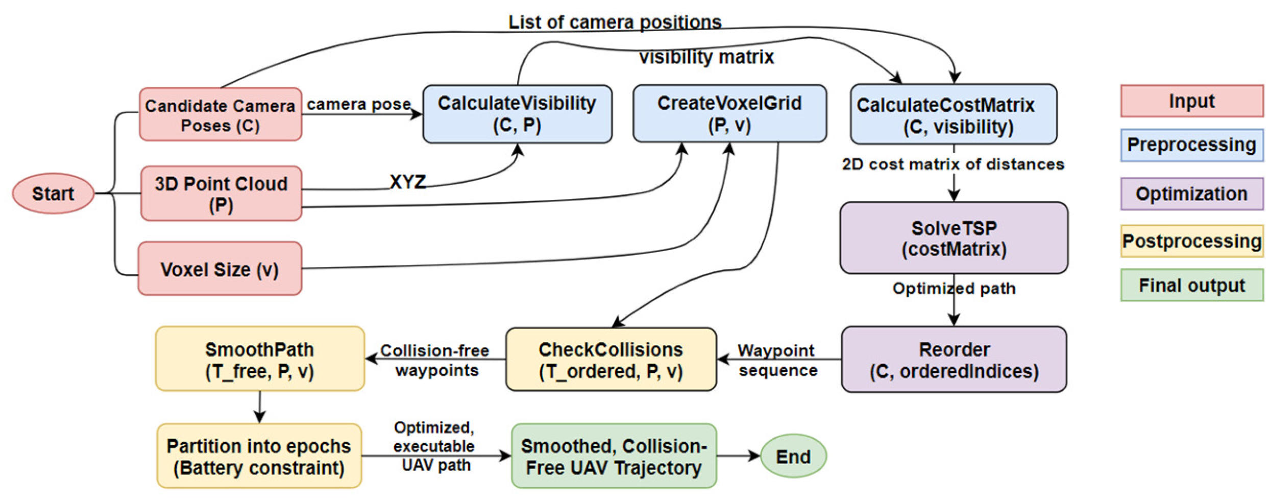
Figure 4.
Comparison of UAV trajectory planning and 3D reconstruction results between the full dense camera network (left) and the ILP-optimized camera network (right) for the bridge inspection experiment.
Figure 4.
Comparison of UAV trajectory planning and 3D reconstruction results between the full dense camera network (left) and the ILP-optimized camera network (right) for the bridge inspection experiment.
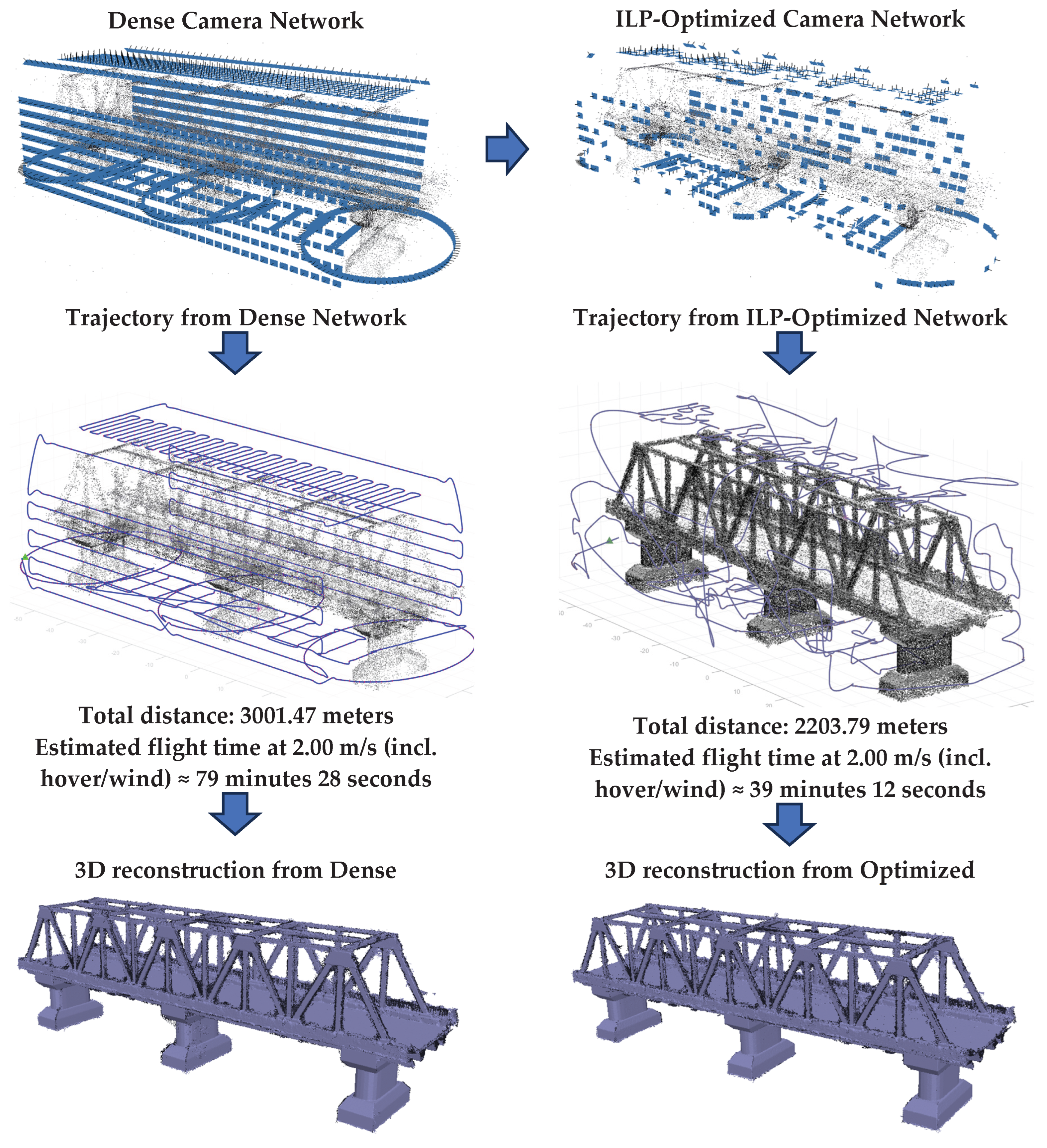
Figure 5.
UAV trajectory optimization results for the steel bridge experiment. (Left) The full TSP-optimized trajectory (blue) covers all waypoints in a single continuous path, which exceeds the UAV’s endurance. (Right) Partitioned trajectory into two epochs (colored), each respecting the endurance constraint.
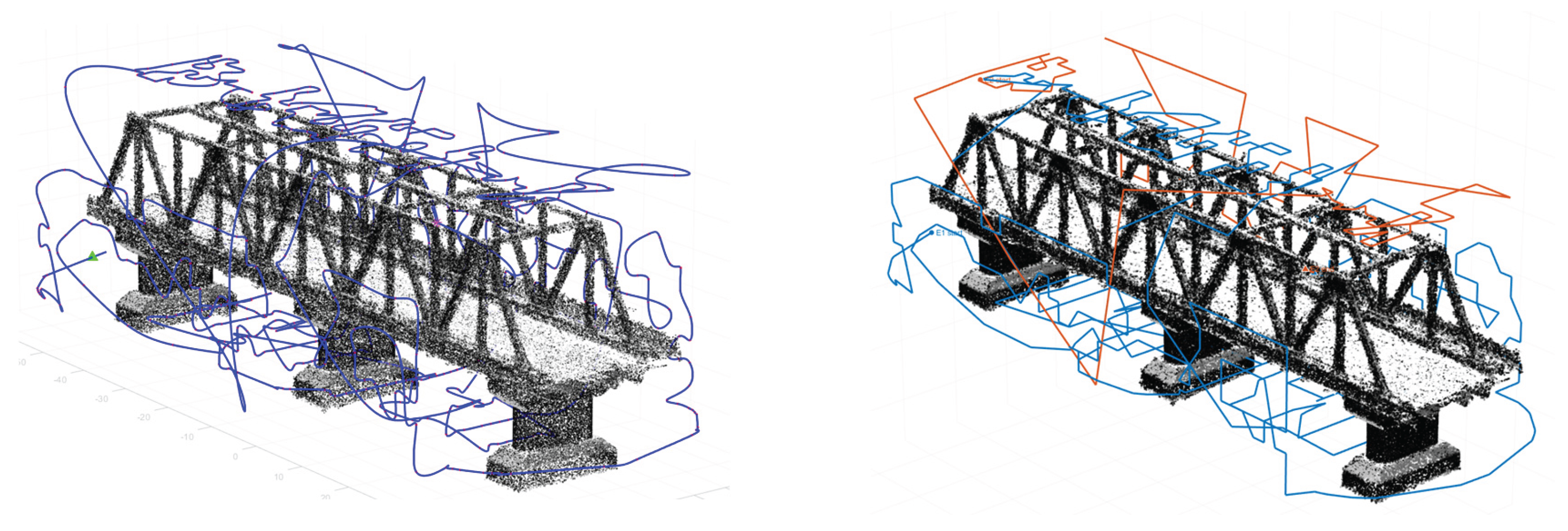
Figure 6.
Comparison of UAV trajectory planning and 3D reconstruction results between the full dense camera network (left) and the ILP-optimized camera network (right) for the industrial facility inspection experiment.
Figure 6.
Comparison of UAV trajectory planning and 3D reconstruction results between the full dense camera network (left) and the ILP-optimized camera network (right) for the industrial facility inspection experiment.
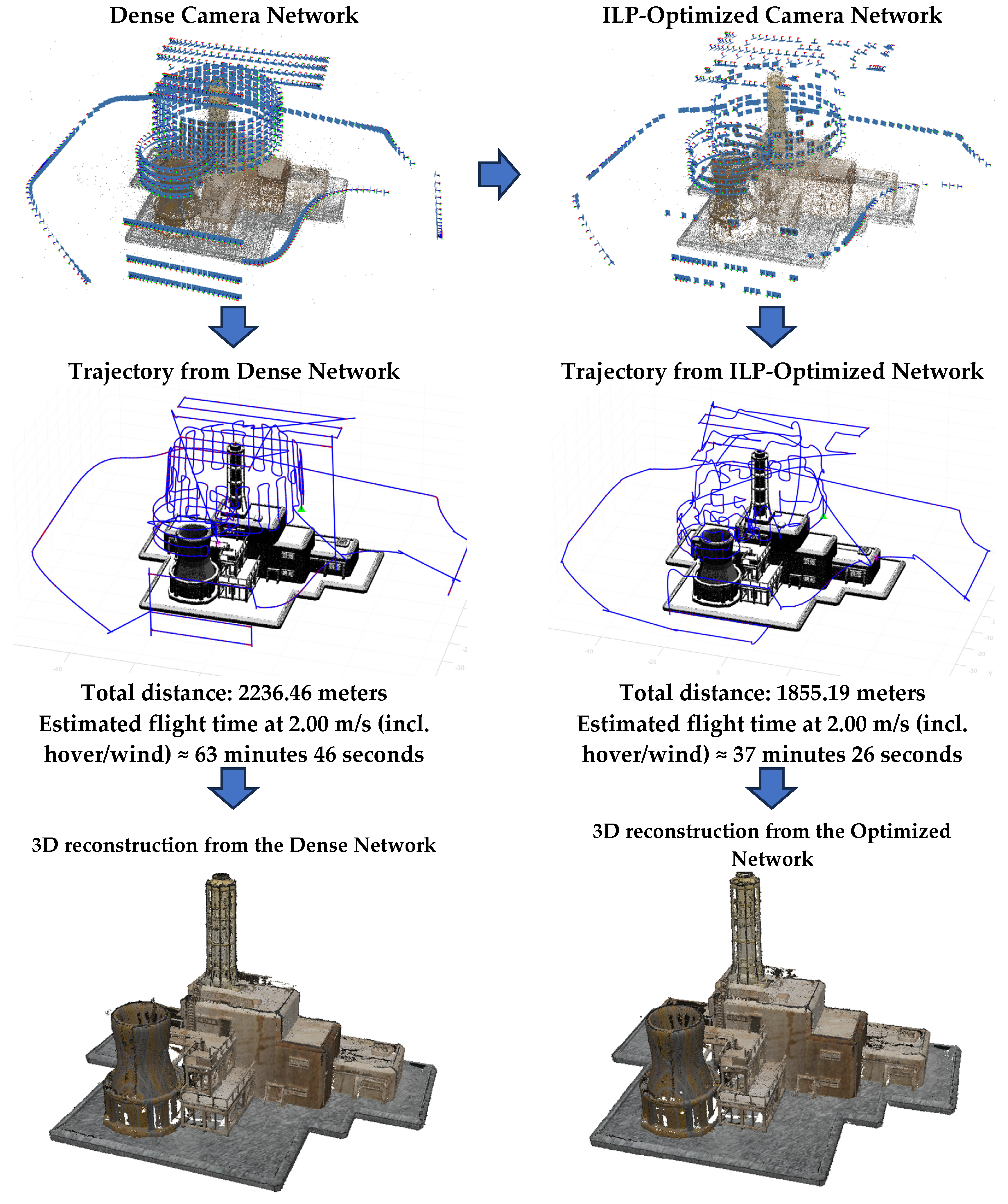
Figure 7.
Optimized UAV trajectories for the industrial plant experiment. (Left) Single continuous TSP trajectory (blue) covering all waypoints, exceeding UAV endurance. (Right) Partitioned trajectory into two epochs (colored), enabling feasible execution within battery constraints.
Figure 7.
Optimized UAV trajectories for the industrial plant experiment. (Left) Single continuous TSP trajectory (blue) covering all waypoints, exceeding UAV endurance. (Right) Partitioned trajectory into two epochs (colored), enabling feasible execution within battery constraints.
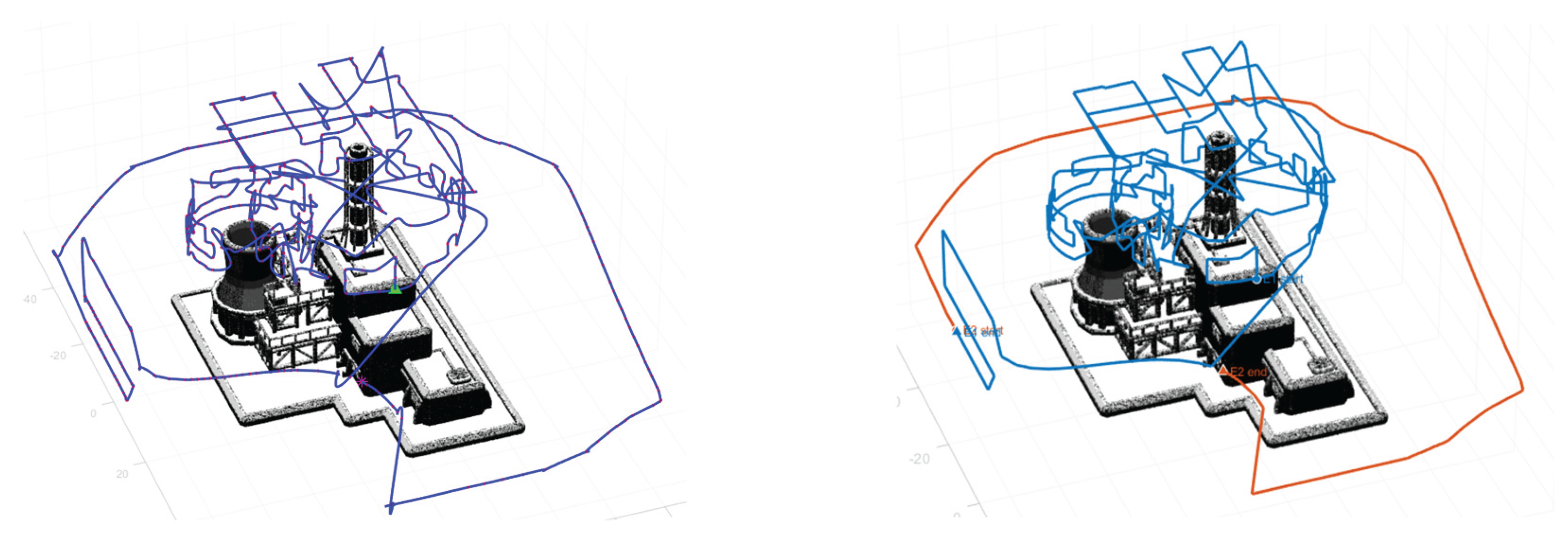
Figure 8.
BIM of the construction site and extracted columns (blue).
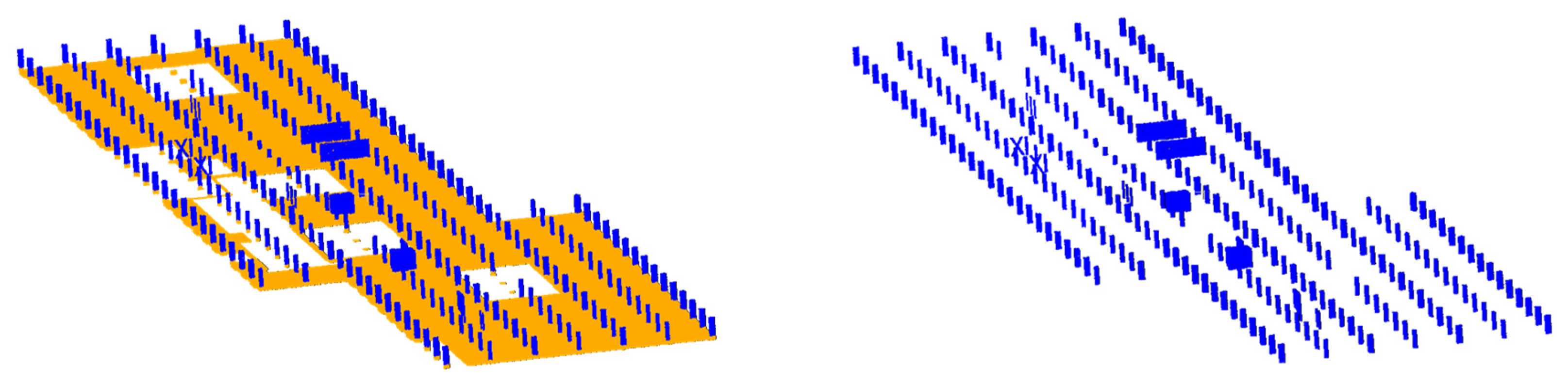
Figure 9.
Comparison of UAV trajectory planning and 3D reconstruction results between the full dense camera network (left) and the ILP-optimized camera network (right) for the indoor construction inspection experiment.
Figure 9.
Comparison of UAV trajectory planning and 3D reconstruction results between the full dense camera network (left) and the ILP-optimized camera network (right) for the indoor construction inspection experiment.
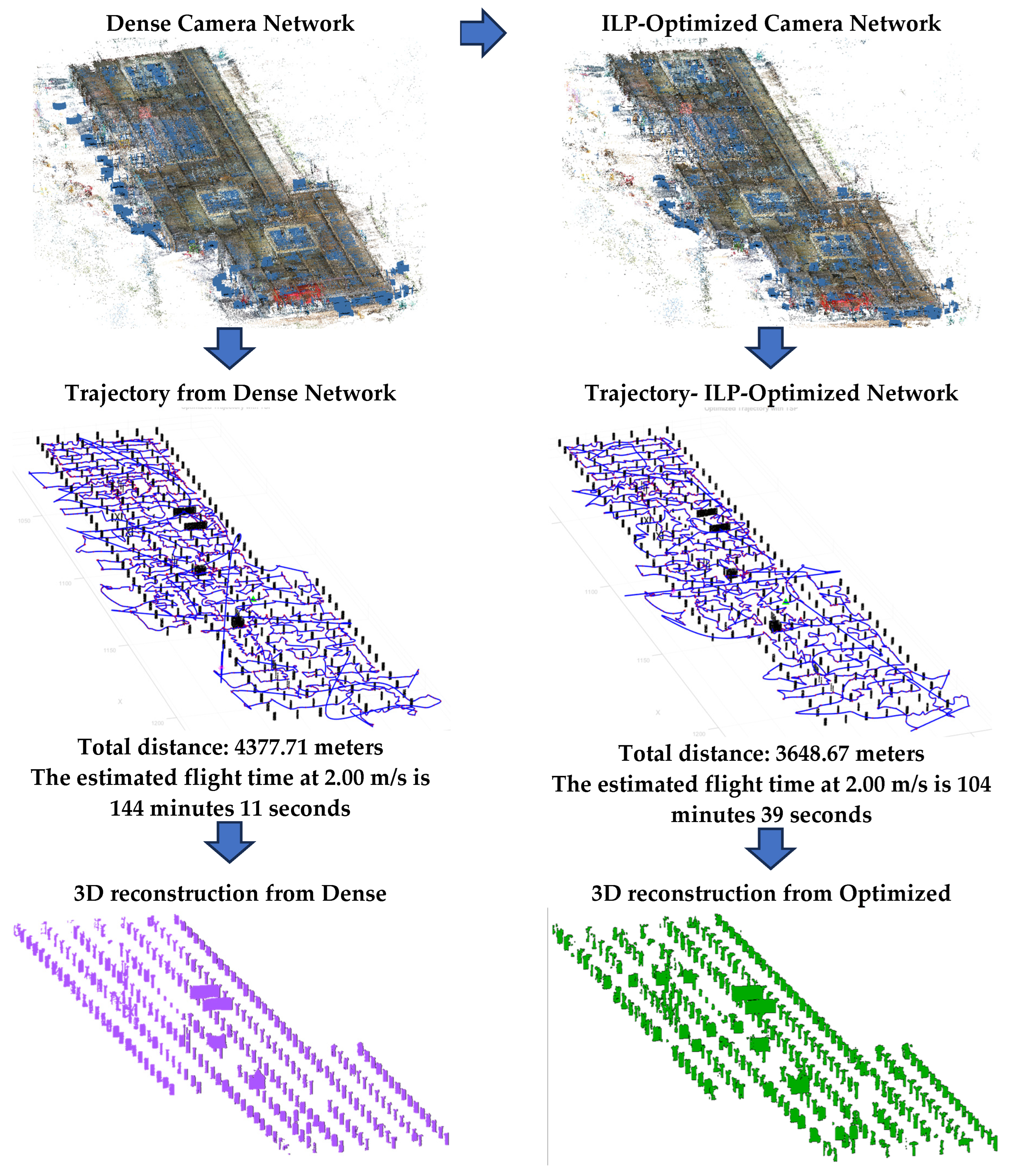
Figure 10.
Partitioning of the optimized UAV trajectory into battery-constrained epochs of the 3rd experiment. (Left) Globally optimized TSP route as a single continuous trajectory. (Right) The same route is divided into four epochs, each highlighted with a distinct color, ensuring that every flight leg remains within the 30-minute endurance limit.
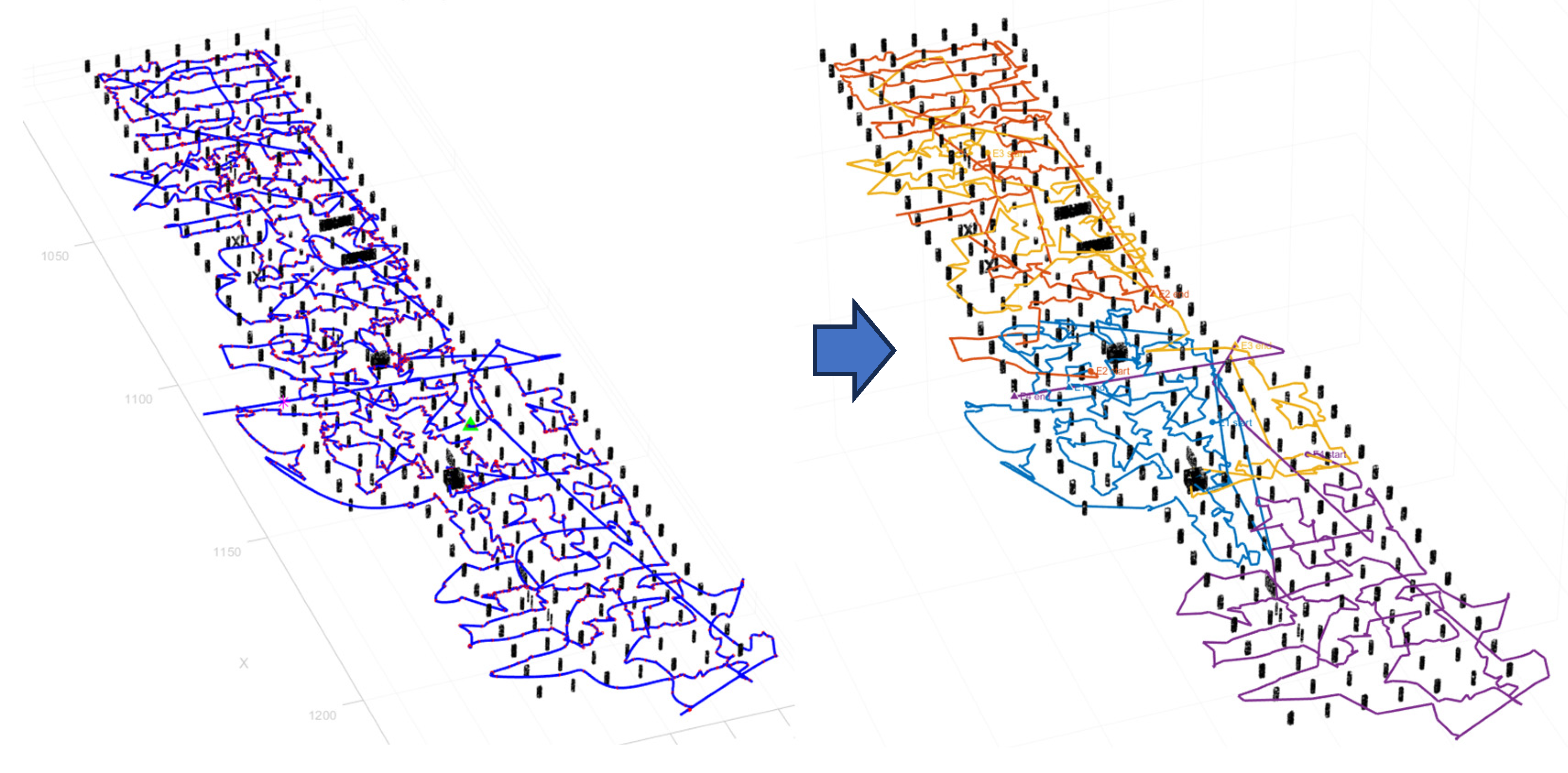
Table 1.
Comparison of selected viewpoint/trajectory planning approaches in UAV photogrammetry and construction inspection.
Table 1.
Comparison of selected viewpoint/trajectory planning approaches in UAV photogrammetry and construction inspection.
| Category | Viewpoint Selection | Trajectory Planning | Constraints | BIM/IFC | Limitations |
|---|---|---|---|---|---|
| Heuristics / Grid-based [5,6] | Uniform/heuristic sampling | Sequential / ad hoc | ✗ | ✗ | Redundant, poor geometry, and long missions |
| Sequential Filtering [7,8] | Dense views are pruned sequentially. | – | Partial (coverage, angular diversity) | ✗ | Heavy; not scalable |
| Set-cover / Submodular Models [10,11,12] | Formal optimization (coverage-based) | Often decoupled / heuristic | Partial (coverage focus) | ✗ | Limited metrics, weak UAV link |
| NBV / Exploration-based [13,14] | Iterative/adaptive sampling | Online replanning (RRT*, horizon) | ✗ (focus on coverage/uncertainty) | ✗ | Model-free; no global coverage guarantee; may get stuck in local minima; costly; less repeatable. |
| Digital Twin / Model-driven [15,16] | Model-guided / quality-predicted | Ad hoc / separate | Some (image sharpness, utility) | Partial | Paths are not globally optimized |
| This Work: BIM-aware ILP + TSP | Global ILP over BIM candidates | TSP-based, battery-feasible | ✓ (B/H, GSD, triangulation) | (direct IFC linkage) | Assumes accurate BIM; outdoor effects not yet modeled |
Table 2.
Quality metrics for Experiment 1: Full Dense Network vs ILP Optimization.
| Metric | Full Dense Network | ILP Optimization |
|---|---|---|
| Mean X Accuracy (m) | 0.004 | 0.006 |
| Mean Y Accuracy (m) | 0.004 | 0.005 |
| Mean Z Accuracy (m) | 0.006 | 0.007 |
| Coverage Adequacy | 0.97 | 0.97 |
| Redundancy Ratio | 0.90 | 0.72 |
| Network Efficiency | 0.00 | 0.62 |
| Mean Cameras per Point | 17 | 8 |
| Max Cameras per Point | 139 | 54 |
| Images to Process | 1522 | 567 |
| Estimated Batteries | 3 | 2 |
Table 3.
Partitioning of the optimized UAV trajectory for the steel bridge experiment .
| Epoch | Waypoints | Duration (min) | Distance (m) |
|---|---|---|---|
| 1 | 433 | 27.0 | 1349.8 |
| 2 | 134 | 10.9 | 712.7 |
Table 4.
Quality metrics for Experiment 2.
| Metric | Full Dense Network | ILP Optimization |
|---|---|---|
| Mean X Accuracy (m) | 0.015 | 0.021 |
| Mean Y Accuracy (m) | 0.011 | 0.019 |
| Mean Z Accuracy (m) | 0.017 | 0.020 |
| Coverage Adequacy | 0.55 | 0.55 |
| Redundancy Ratio | 0.95 | 0.89 |
| Network Efficiency | 0.00 | 0.52 |
| Mean Cameras per Point | 15 | 7 |
| Max Cameras per Point | 320 | 157 |
| Images to Process | 1263 | 606 |
| Estimated Batteries | 3 | 2 |
Table 5.
Battery-constrained partitioning of the optimized trajectory for the industrial plant experiment.
Table 5.
Battery-constrained partitioning of the optimized trajectory for the industrial plant experiment.
| Epoch | Waypoints | Duration (min) | Distance (m) |
|---|---|---|---|
| 1 | 444 | 27.0 | 1309.0 |
| 2 | 162 | 8.6 | 335.1 |
Table 6.
Quality metrics for Experiment 3.
| Metric | Full Dense Network | ILP Optimization |
|---|---|---|
| Mean X Accuracy (m) | 0.003 | 0.004 |
| Mean Y Accuracy (m) | 0.002 | 0.003 |
| Mean Z Accuracy (m) | 0.001 | 0.001 |
| Coverage Adequacy | 1.00 | 0.99 |
| Redundancy Ratio | 0.96 | 0.94 |
| Network Efficiency | 0.00 | 0.31 |
| Mean Cameras per Point | 36 | 24 |
| Max Cameras per Point | 144 | 98 |
| Images to Process | 3025 | 2078 |
| Estimated Batteries | 6 | 4 |
Table 7.
Battery-constrained partitioning of the optimized trajectory for the real construction experiment.
Table 7.
Battery-constrained partitioning of the optimized trajectory for the real construction experiment.
| Epoch | Waypoints | Duration (min) | Distance (m) |
|---|---|---|---|
| 1 | 583 | 27.0 | 748.6 |
| 2 | 586 | 27.0 | 736.8 |
| 3 | 541 | 27.0 | 914.6 |
| 4 | 363 | 20.0 | 837.4 |
Disclaimer/Publisher’s Note: The statements, opinions and data contained in all publications are solely those of the individual author(s) and contributor(s) and not of MDPI and/or the editor(s). MDPI and/or the editor(s) disclaim responsibility for any injury to people or property resulting from any ideas, methods, instructions or products referred to in the content. |
© 2025 by the authors. Licensee MDPI, Basel, Switzerland. This article is an open access article distributed under the terms and conditions of the Creative Commons Attribution (CC BY) license (http://creativecommons.org/licenses/by/4.0/).
Copyright: This open access article is published under a Creative Commons CC BY 4.0 license, which permit the free download, distribution, and reuse, provided that the author and preprint are cited in any reuse.


