Submitted:
29 October 2025
Posted:
30 October 2025
You are already at the latest version
Abstract
Corporate bankruptcy prediction has become increasingly critical amid economic uncertainty. This study proposes a novel two-stage machine learning approach to enhance bankruptcy prediction accuracy, applied to Tokyo Stock Exchange-listed companies. First, models were trained using 173 financial indicators. Second, a wrapper-based feature selection process was employed to reduce dimensionality and eliminate noise, thereby identifying an optimal seven-feature set. Two ensemble learning methods, Random Forest and LightGBM, were used. Random Forest correctly predicted 566 bankruptcies using the reduced feature set (88 more than when using all features) compared with 451 by LightGBM (31 more than when using all features). The study also addresses challenges posed by imbalanced data by employing resampling techniques (SMOTE, SMOTE-ENN, and KMeans). Additionally, the need for industry-specific modeling is recognized by constructing models for the six industry sectors. These findings highlight the importance of feature selection and ensemble learning for improving model generalizability and uncovering industry-specific patterns. This study contributes to the field of bankruptcy prediction by providing a robust framework for accurate and interpretable predictions for both academic research and practical applications. Future work will focus on further enhancing prediction accuracy to identify more potential bankruptcies.
Keywords:
corporate bankruptcy prediction
; feature selection
; ensemble learning
; random forest
; LightGBM
; imbalanced data
; Tokyo Stock Exchange
1. Introduction
In today’s increasingly uncertain environment, corporate management faces significant challenges due to the heightened risk of bankruptcy arising from deteriorating business performance. Bankruptcies impose substantial losses on stakeholders, including business partners, investors, and financial institutions. Accordingly, developing models that prevent or enable the early detection of bankruptcy has become essential. While traditional research has relied on statistical approaches, recent advances in machine learning have enabled more objective and accurate predictions.
This study builds on earlier work by applying ensemble learning methods—Random Forest and LightGBM—while addressing key challenges such as feature selection, imbalanced data, and industry-specific modeling. In particular, the study integrates resampling techniques with stepwise feature selection, thereby enhancing model generalization, interpretability, and the ability to uncover sector-specific bankruptcy patterns.
Corporate bankruptcy prediction has long attracted scholarly and practical attention. Foundational studies, including Beaver (1966), Altman (1968), Ohlson (1980), and Zmijewski (1984), demonstrated the predictive power of accounting ratios and introduced discriminant and probit/logit models (Nam and Jinn, 2000). Subsequent refinements included hazard models (Shumway, 2001), industry effects (Chava and Jarrow, 2004), market-based indicators (Hillegeist et al., 2004; Wu, Gaunt, and Gray, 2010), and hybrid approaches integrating accounting, market, and macroeconomic variables (Hernández Tinoco and Wilson, 2013; Ciampi, 2015; Martín and Rojo, 2019). Altman himself and subsequent studies have proposed variations of the Z-score model to extend its applicability to non-manufacturing firms, private companies, and firms in emerging markets (Altman et al., 2017). Lin and McClean (2001) and Varetto (1998) applied data mining and genetic algorithms, while Sun and Shenoy (2007) employed Bayesian networks. Huang et al. (2004) conducted a comparative study using support vector machines and neural networks for credit rating analysis, highlighting the effectiveness of advanced machine learning techniques for financial risk assessment. More recently, Choi and Lee (2018) applied multi-label learning techniques for corporate bankruptcy prediction, demonstrating the potential of advanced machine learning methods to handle multiple bankruptcy indicators simultaneously. These studies provided interpretability but faced limitations in capturing nonlinearities and complex interactions.
Since the 2000s, machine learning has transformed bankruptcy prediction. Ensemble methods, including Breiman’s (2001) Random Forest and Dietterich’s (2000) ensemble strategies, demonstrated the advantages of combining classifiers. Boosting algorithms such as AdaBoost (Heo and Yang, 2014), Gradient Boosting (Chen and Guestrin, 2016), and LightGBM (Ke et al., 2017) proved highly effective. Hybrid frameworks integrated multiple learners (Wang et al., 2010; Tang and Yan, 2021; Yu and Zhang, 2020), while CatBoost-based models further enhanced accuracy (Ben Jabeur et al., 2021; Mishra and Singh, 2022). Comparative studies confirm that ensemble models consistently outperform single classifiers in both stability and predictive performance (Bandyopadhyay and Lang, 2013; Lahsasna et al., 2018; Lee and Chen, 2020; Kraus and Feuerriegel, 2019; Guillén and Salas, 2021). Stacking and meta-learning frameworks have also been proposed (Tsai and Hsu, 2013; Tang, Zhang, and Chawla, 2009). Moreover, multi-industry frameworks such as Lee and Choi (2013) demonstrate the importance of accounting for sectoral heterogeneity in model design.
A persistent methodological challenge is class imbalance. Bankruptcies are rare compared with solvent cases, and classifiers trained on such datasets often achieve inflated accuracy while failing to capture true defaults. Early work by He and Garcia (2009) and Huang and Ling (2005) highlighted methodological biases, and later studies proposed over- and under-sampling approaches. SMOTE (Chawla et al., 2002), SMOTE-ENN (Batista et al., 2004; Liu and Wu, 2021), and SMOTE-IPF (Sáez et al., 2015) effectively rebalance class distributions. Undersampling approaches such as exploratory undersampling (Liu, Wu, and Zhou, 2009) provided alternatives. Reviews confirm the importance of these methods (Fernandez, García, and Herrera, 2018; Fernández et al., 2018; Sun et al., 2014). Neural network studies further revealed imbalance sensitivity (Buda, Maki, and Mazurowski, 2018). More recent work integrated rebalancing with ensemble learning (Zhao and Wang, 2018; Shetty, Musa, and Brédart, 2022). Recent advances also include hybrid approaches that integrate evolutionary algorithms with domain adaptation (Ansah-Narh et al., 2024).
Feature engineering and dimensionality reduction are also critical. While early studies relied on accounting ratios, more recent work incorporated diverse features such as governance (Ciampi, 2015), market variables, and macroeconomic indicators (Sun et al., 2014). Feature selection reduces noise and overfitting (Guyon and Elisseeff, 2003; Tsai, 2009; Jain and Johnson, 2020). Hybrid strategies (Ko, Kim, and Kang, 2021; Pramodh and Ravi, 2016; Hossari and Rahman, 2022; Kotze and Beukes, 2021; García et al., 2019), explainable AI (Lundberg and Lee, 2017; Wu and Wang, 2022; Zhang and Wang, 2021; Giudici and Hadji-Misheva, 2022; Yeh, Chi, and Lin, 2022), and advances in scikit-learn (Pedregosa et al., 2011) have further improved transparency and reproducibility. In addition, Dikshit and Pradhan (2021) demonstrated the applicability of interpretable models in environmental risk prediction, highlighting the transferability of explainable AI across domains.
Deep learning has expanded the methodological toolkit. Neural networks were introduced by Atiya (2001), Lin, Chiu, and Tsai (2010), and Kim (2011), with more recent contributions focusing on sequential and attention-based models (Li, Sun, and Wu, 2022; Kim, Cho, and Ryu, 2022). Ensemble deep learning reviews further highlight the growing promise of these methods (Ganaie and Hu, 2022). BERT adaptations extend to textual features (Kim and Yoon, 2023), while hybrid frameworks combine neural networks with market and macroeconomic data (Zhang and Wang, 2021). Comparative studies highlight their growing competitiveness (Iparraguirre-Villanueva and Cabanillas-Carbonell, 2023). Industry- and country-specific determinants remain key: Korean construction (Heo and Yang, 2014), French SMEs (Mselmi, Lahiani, and Hamza, 2017), crisis contexts (Nam and Jinn, 2000; Narvekar and Guha, 2021), dotcom failures (Chandra, Ravi, and Bose, 2009), firm size and volatility in Pakistan (Rashid, Hassan, and Karamat, 2021), policy uncertainty (Fedorova et al., 2022), and early banking distress detection (Ravisankar and Ravi, 2010) further illustrate contextual variation.
Several meta-studies have synthesized these developments. Bellovary, Giacomino, and Akers (2007) reviewed early research, while Ravi Kumar and Ravi (2007), Alaka et al. (2018), Sun et al. (2014), and Dasilas and Rigani (2024) provided systematic reviews. Xu and Ouenniche (2018) applied DEA benchmarking, Radovanovic and Haas (2023) assessed socio-economic costs, and Razzak, Imran, and Xu (2019) reviewed deep learning for credit scoring. Succurro, Arcuri, and Costanzo (2019) introduced robust PCA, and Sánchez-Medina et al. (2024) investigated bankruptcy resolution prediction. Wu, Gaunt, and Gray (2010) compared alternative models, while Yeh and Lien (2009) analyzed credit card default risks in relation to corporate bankruptcy prediction. Du Jardin (2016) further demonstrated the effectiveness of a two-stage classification strategy, motivating the two-stage approach of this study.
Overall, the literature reveals a clear progression from interpretable statistical models to increasingly complex, data-driven, and explainable frameworks. Prediction success depends not only on algorithmic choice but also on handling imbalanced data, selecting informative features, and incorporating industry-specific determinants. Building on this understanding, the present study adopts a two-stage machine learning framework for bankruptcy prediction among Tokyo Stock Exchange–listed firms. In the first stage, comprehensive learning is performed using 173 financial indicators. In the second stage, wrapper-based feature selection is applied to gradually reduce dimensionality, eliminate noise, and arrive at an optimal seven-feature set. This approach enhances both predictive performance and interpretability.
To capture sector-specific heterogeneity, separate models are constructed for six industries—Construction, Real Estate, Services, Retail, Wholesale, and Electrical Equipment—thus uncovering sectoral bankruptcy determinants and patterns. In addition, three resampling techniques—SMOTE, SMOTE-ENN, and k-means clustering—are incorporated to address class imbalance. Empirical results reveal that Random Forest correctly predicts 566 bankruptcies and LightGBM predicts 451, both substantially outperforming models without feature reduction. By simultaneously addressing four key challenges—methodological choices, dataset design, class imbalance, and industry heterogeneity—this study underscores both its novelty and practical relevance.
2. Materials and Methods
2.1. Machine Learning Methods
This study employs Random Forest and LightGBM. Brief explanations of each method follow.
2.1.1. Random Forest
Random Forest is a machine learning framework based on decision-tree algorithms. It uses bagging, which is a type of ensemble learning, to create high-accuracy learners. Bagging trains multiple ‘weak learners’ in parallel using bootstrapping. Bootstrapping extracts data samples with replacement from the original dataset. Since sampling with replacement allows for duplicates, the same data point may be selected multiple times for training a single weak learner. Bagging uses bootstrapping to train multiple weak learners in parallel. Bootstrapping involves resampling with replacement from the original dataset. Each learner performs learning and prediction independently; for regression tasks, learner predictions are averaged, and for classification tasks, a majority vote determines the final prediction.
2.1.2. LightGBM
LightGBM is also a machine learning framework based on decision tree algorithms. It employs gradient boosting, an ensemble-learning method, to create high-accuracy learners. This approach constructs a ‘strong learner’ by sequentially combining individual learners. Specifically, it uses the steepest descent method to minimize the error between predicted and actual numbers. XGBoost, a conventional machine learning algorithm that uses gradient boosting, employs a level-wise tree-growth strategy to grow decision trees. This method grows a decision tree by expanding its levels (layers). In contrast, LightGBM employs leaf-wise growth, which grows decision trees by expanding the tree’s leaves. This enables LightGBM to achieve faster processing, while maintaining XGBoost’s accuracy.
2.2. Evaluation Metrics
Evaluation metrics are quantitative indicators used to assess model performance. Using evaluation metrics helps to determine how accurately the constructed model can predict bankruptcy from the input data. Furthermore, evaluation metrics play a crucial role in comparing model performance and facilitating improvements.
The following evaluation metrics are used in this study. We define true positives (TPs) as instances when bankrupt companies are correctly predicted as bankrupt; false negatives (FNs) as instances when bankrupt companies are incorrectly predicted as non-bankrupt; true negatives (TNs) as instances when non-bankrupt companies are correctly predicted as non-bankrupt; and false positives (FPs) as instances when non-bankrupt companies are incorrectly predicted as bankrupt. Using these TPs, FPs, TNs, and FNs, we calculate the following metrics: precision, accuracy, recall, false positive rate, and false negative rate. Given our focus on bankruptcy, TPs are our primary metric to represent correctly predicted bankrupt companies. Therefore, we consider the model that yielded the highest number of TPs as the best. We compute recall as the evaluation metric for industry-specific bankruptcy prediction, considering different dataset compositions and resampling methods. Since the actual number of bankrupt companies varies by industry, TPs alone cannot determine prediction accuracy. Assessing recall therefore provides a better understanding of bankruptcy prediction accuracy for each industry.
2.3. Numerical Experiment Design
2.3.1. Datasets
We construct models for six industries based on the Tokyo Stock Exchange’s sector classifications: construction, real estate, services, retail, wholesale, and electrical equipment. Data were obtained from the financial statements of companies listed on the Tokyo Stock Exchange, using the Nikkei NEEDS database. In this study, we define bankruptcy as a company being delisted owing to civil rehabilitation proceedings or similar events. We use data from 317 companies that filed for bankruptcy between 1991 and 2021.
Table 1 presents three study datasets with different numbers of features. Numbers in parentheses indicate the feature counts. The significant disparity between the numbers of non-bankrupt and bankrupt companies indicates an imbalanced dataset. The first dataset configuration contains data from 52,950 companies and uses only financial indicators as features. The second configuration contains data from 26,674 companies. This dataset augments the short-term financial performance indicators from the first dataset with investment-financing network indicators representing financing diversity and long-term intercompany trust relationships. The third dataset, constructed for benchmarking against the first (financial) and second (investment-financing) datasets, includes data from 26,674 companies. This is derived by stripping the 12 investment-financing network indicators from the second dataset, leaving 161 purely financial features. Consequently, it differs from the first dataset in terms of size (26,674 vs. 52,950 companies) and from the second in terms of feature count (161 vs. 173 features).
2.3.2. Indicators
We utilize all 161 financial indicators available from the Nikkei NEEDS-Financial QUEST (FQ), a comprehensive economic database service. Following the NEEDS-FQ classification system, these indicators are categorized into seven types: profitability, return on capital, margin-related, productivity, stability, growth, and cash flow indicators (Table 2).
2.3.3. Investment-Financing Network Indicators
We calculate investment-financing network indicators from networks representing corporate investment and financing relations. To construct these networks, we use data from the Nikkei NEEDS-Financial QUEST on major shareholders, corporate shareholdings, and loans. Specifically, we calculate six investment network indicators and six financing network indicators, totaling 12 indicators.
We define each indicator as follows:
- Degree centrality: How connected a given node is to other nodes in a network.
- Betweenness centrality: The frequency with which a given node lies on the shortest path between other nodes, indicating the degree of connection between the node and others.
- Network density: The degree of connection among nodes, expressed as a ratio. The denominator is the number of possible connections, and the numerator is the number of actual connections.
- Authority score: The extent to which other nodes link to a given node, representing how many other nodes are linked to it.
- Hub score: Outgoing edge connections to other nodes.
- PageRank: The importance of a webpage.
2.3.4. Computational Environment
Before running the models with LightGBM and Random Forest, we perform data standardization as a preprocessing step. Next, we conduct a 10-fold cross-validation to optimize the hyperparameters using Optuna, a Python package. The prediction models are then constructed using the optimized parameters. Table 3 and Table 4 present the corresponding hardware and software specifications.
3. Results
In this two-stage study, the results of the second stage are derived from
a dataset of seven features obtained through progressive feature reduction of
the 173-feature set used in the first stage. This eliminates noise and prevent
overfitting. We use the feature importance attribute to determine which features
the models rely on the most for bankruptcy prediction, quantifying each
feature’s importance and visualizing the results.
3.1. First Stage Results (173 Features)
This section presents the results of the first stage of bankruptcy
prediction. In the first stage, we construct bankruptcy prediction models using
Random Forest and LightGBM with a dataset containing all 173 available
financial indicators.
3.1.1. Random Forest
Table
4
presents the results obtained by
dataset configuration using the 173-feature set. The total TP count across the
financial, investment financing, and comparison datasets was 478. Among the
datasets, the financial dataset, having the largest sample size, achieved the
best prediction accuracy, with 284 TPs. Both the investment financing and
comparison datasets yielded 97 TPs, indicating no apparent advantage in using
investment financing network indicators.
Resampling:
For the 317 bankrupt companies across the six industries (
Table 5
),
k-means achieved the highest accuracy with 186 TPs across all three datasets,
followed by SMOTE-ENN with 177 TPs, and SMOTE with 115 TPs.
Industry-Specific
Results:
Table 6
presents the industry-specific prediction
results by dataset configuration. The highest TP count (75) was recorded in the
construction industry when the financial dataset was used. By contrast, the
lowest TP count (0) was recorded for the wholesale industry when using the
comparison dataset.
Resampling Results by
Industry:
Table 7
presents the resampling results by industry.
Applying k-means resampling to the construction industry data yielded the
highest TP count
(5
9
)
,
whereas applying SMOTE resampling to the wholesale industry data produced the
lowest TP count (3).
Taken
together, the results in
Tables 6 and 7
show that applying Random Forest to the data
from the construction industry yields the highest total TP count (152), whereas
applying this method to the wholesale industry data produces the lowest total
TP count (21). Recall was highest in the real estate industry (58.33%) and
lowest in the wholesale industry (26.92%).
Feature Importance: To pinpoint which features were significant for the
model’s predictions, we visualized the feature importance scores assigned by
the Random Forest algorithm.
Figure 1
illustrates the top seven features (out of 173)
for the electrical-equipment industry using the financial dataset with
SMOTE-ENN resampling.
3.1.2. LightGBM
Table
8
presents the results obtained
using 173-feature set. Across the financial, investment-financing, and
comparison datasets, Random Forest correctly identified 420 bankrupt firms, 58
more than LightGBM. When broken down by dataset, Random Forest achieved its
highest TP count on the financial dataset, which had the largest sample size
with 264 TPs, and identified 58 bankrupt firms using the investment-financing
dataset and 97 using the comparison dataset. Notably, we found no significant
differences between the investment-financing dataset and the comparison dataset
when using Random Forest. However, a difference emerged with LightGBM. For
LightGBM, incorporating network indicators resulted in worse performance.
Resampling: Looking at the resampling results across six industries
covering 317 bankrupt companies in total, SMOTE-ENN achieved the highest accuracy
with 149 TPs, followed by SMOTE with 141 TPs, and K-means with 129 TPs (
Table 9
).
Industry-Specific
Results:
Table 10
presents the prediction results categorized by
industry and dataset configuration. The financial dataset for the real estate
industry produced the highest TP count with 62 companies, whereas the
investment-financing dataset for the electrical equipment industry showed the
lowest TP count of 0.
Resampling
Results by Industry:
Table 11
presents the resampling results for each
industry. The highest TP count (49) was generated by the construction industry
using SMOTE-ENN. Conversely, the lowest TP count (11) is observed for the
service industry using both SMOTE-ENN and k-means.
The
combined results in
Tables 10 and 11
show that, when using LightGBM, 139 TPs were
generated for the real estate industry. By contrast, the lowest TP count (34)
was observed in the service industry. Recall was highest in the real estate
industry (60.96 %) and lowest in the wholesale industry (24.
30
%).
Feature Importance: To identify the features that were significant for
the model’s predictions, we visualized the feature importance scores assigned
by LightGBM.
Figure 2
illustrates the top seven features (out of 173)
for the electrical-equipment industry using the financial dataset processed
using SMOTE-ENN.
3.2. Second-Stage Analysis Results (7 Features)
This study proposes a two-stage bankruptcy
prediction model using financial data from listed Japanese companies. The first
stage involved model training, using all 173 available financial indicators.
The second stage improves prediction accuracy through passive dimensionality
reduction to eliminate noise and prevent overfitting. The second stage applies
feature selection using Random Forest and LightGBM to iteratively reduce the
feature set from 173 to a smaller optimal set. The aim is to enhance the model’s
predictive performance by eliminating noise and irrelevant features,
particularly when identifying bankrupt companies. The feature selection process
followed a wrapper-based approach involving iterative model training and
evaluation based on TPs and recall to identify the optimal number of features
for each industry category. The procedure is outlined as follows:
- Step 1: Train the model using all 173 features.
- Step 2: Based on performance (TP count), remove less important features and retain the top features for each industry.
- Step 3: Train a new model using the reduced feature set.
- Step 4: Steps 2 and 3 are repeated until the TP reaches its maximum. Point at which the TP peaks determine the optimal feature set. The results were as follows:
- Among the seven selected features, Random Forest achieved 566 TPs, whereas LightGBM achieved 451. Thus, the Random Forest model predicted 115 more bankruptcies.
In contrast, as previously mentioned, when all 173 features were used,
Random Forest predicted 478 bankruptcies and LightGBM predicted 420. These
results demonstrate that by employing the wrapper-based approach, which was the
key objective of this study, we successfully reduced dimensionality, eliminated
noise, and improved model performance.
Table 12
and
Figure 3
show how the TP count changed as the number of features
was progressively reduced from 173 to two through feature selection,
representing the sum of the SMOTE, SMOTE+ENN, and k-means results.
3.2.1. Random Forest
Table
13
presents the results generated
using the 7-feature set. The total TP count across the financial, investment
financing, and comparison datasets was 566. By contrast, as mentioned
previously, when all 173 features were used, Random Forest achieved 478 TPs.
This demonstrates that using the seven selected features predicted 88 more
bankruptcies (566 vs. 478 TPs) with Random Forest than using all 173 features.
Thus, we successfully achieved our study’s objective of improving bankruptcy
prediction accuracy. Considering the results by dataset configuration, the
financial dataset, which had the largest sample size, showed the best
prediction accuracy, with 303 TPs. The model produced 142 TPs with the investment
financing dataset and 121 TPs with the comparison dataset, which demonstrates
the added value of incorporating investment financing network indicators.
Resampling:
SMOTE-ENN resampling achieved the highest accuracy, with 211 TPs across all
three datasets combined (
Table 14
). K-means followed with 206 TPs and SMOTE with
149 TPs. In comparison, when all 173 features were used, SMOTE, SMOTE-ENN, and
K-means achieved 115, 177, and 186 TPs, respectively, indicating improvements
of 34, 34, and 20 additional TPs, respectively, with the seven-feature set
compared with all 173 features.
As shown in
Table 15
,
the Random Forest model achieved the highest number of TPs when applied to the
financial dataset of the construction industry. Specifically, it correctly
identified 87 bankrupt firms out of 126 actual bankruptcies.
In
contrast, the comparative dataset exhibited the lowest performance in the
service industry, with only two TPs.
Resampling
Results by Industry:
Table 16
presents the resampling results for each
industry. In the construction industry, SMOTE-ENN yields the highest TP count
of 67. Conversely, for the wholesale industry, using SMOTE resulted in the
lowest TP count at only 12.
The combined results in
Tables 15 and 16
indicate that the highest TP count (172) was recorded for the
construction industry, whereas the lowest TP count (48) was recorded for the
wholesale industry. In terms of recall, the highest rate (68.8
6
%)
was observed for the real estate industry data, whereas the lowest rate (
54.29
%)
was observed for the
service
industry data.
Feature
Importance:
Table 17
compares the top seven features identified by
Random Forest from the full 173-feature set with the seven features selected
for the optimized model. This table highlights the top seven features selected
from the original 173 features for comparison.
Notably, no network indicators were selected among the final seven
features, and all the selected features were financial indicators. Furthermore,
Cash Flow to Net Interest-Bearing Debt Ratio and Net Interest Burden to Sales
Ratio appear among the seven selected features and among the top seven
indicators of the 173-feature set, demonstrating their importance for
bankruptcy prediction with Random Forest. Moreover, when using the
seven-feature set, two cash flow indicators are included: cash flow to net interest-bearing
debt ratio and operating cash flow to sales ratio. When using all 173 features,
four of the top seven features are cash flow-related: the Cash Flow to Net
Interest-Bearing Debt Ratio, Dividends to Cash Flow Ratio, Cash Flow to
Long-Term Debt Ratio, and Cash Flow to Fixed Liabilities Ratio. Given that cash
shortages are often the primary cause of corporate bankruptcy, this finding
indicates that the model successfully identifies the relevant features.
For the electrical
equipment industry,
Figure 4
presents the importance scores of the
top
seven features computed on the financial dataset following SMOTE-ENN
resampling.
3.2.2. LightGBM
Table
18
presents the results obtained
using these seven features. Among the datasets, the highest prediction accuracy
for 283 TPs was achieved using the financial dataset with the largest sample
size.
Resampling:
Across all six industries and three dataset configurations (encompassing 317
bankrupt companies in total), SMOTE resampling achieved the highest accuracy
with 199 TPs, followed by SMOTE-ENN with 191 TPs, and k-means with 61 TPs.

Table 19.
LightGBM true positive count by resampling method and dataset configuration.
| Resampling | Actual | Predicted | |||
|---|---|---|---|---|---|
| Total | Financial | Investment-financing | Comparison | ||
| SMOTE | 317 | 199 | 116 | 44 | 39 |
| SMOTE-ENN | 317 | 191 | 114 | 41 | 36 |
| K-means | 317 | 61 | 53 | 2 | 6 |
| Total | 951 | 451 | 281 | 87 | 81 |
Industry-Spe
cific Results :As shown in
Table 20
,
for LightGBM, the highest TP count (72) is achieved using the financial dataset
for the real estate industry, whereas the lowest TP count of 2 is observed when
using the investment-financing dataset for the retail industry.
Resampling
Results by Industry: As shown in
Table 21
, which presents the LightGBM resampling results
by industry, SMOTE-ENN yielded 60 TPs with data for the real estate industry.
K-means showed the worst performance with the electrical equipment industry
data at zero TPs.
As
the combined results in
Tables 20 and 21
show, when the seven-feature LightGBM model is
applied across industries, the highest TP count (138) is predicted for the real
estate industry. Conversely, the lowest TP count of 43 is predicted for the
service industry. In terms of recall, the highest rate was recorded for the
construction industry (68.57 %), whereas the lowest rate was observed for the
wholesale industry (33.70 %).
Feature Importance:
Table 22
presents a comparison of the top seven features
identified by LightGBM from the full 173-feature set with the seven features
selected for the optimized model. The Depreciation to Sales ratio feature
appears in both the seven selected features and the top seven of the full set,
underscoring its critical role in LightGBM-based bankruptcy pre- diction. In
the seven-feature model, four cash flow metrics were selected (dividend-to-free
cash flow ratio, instant coverage cash flow, cash flow to debt ratio, and cash
flow to current liabilities ratio), whereas in the full 173-feature ranking,
the Cash Flow to Net Interest-Bearing Debt Ratio also emerged among the top
indicators. Given that insufficient cash flow is the leading cause of corporate
bankruptcies, these results confirm that the proposed approach effectively
identified relevant features.
Figure 5
illustrates the top seven features
(out of 173) for the electrical equipment industry when using a financial
dataset processed with SMOTE-ENN.
4. Discussion
This study contributes significantly to the field of bankruptcy
prediction by proposing a novel two-stage machine learning approach that
integrates ensemble learning, feature selection, and industry-specific
analysis. By employing Random Forest and LightGBM, this research addresses
critical challenges in bankruptcy prediction, including handling
high-dimensional financial data, imbalanced datasets, and the need for
industry-specific modeling. The innovative wrapper-based feature selection
process effectively reduced the dimensionality of the dataset from 173
financial indicators to seven optimal features, thereby eliminating noise and
enhancing model performance.
Furthermore, we construct industry-specific models for six sectors based
on the Tokyo Stock Exchange classification, uncovering unique bankruptcy
patterns and causes within each industry. This approach not only improves the
generalizability of the models but also provides actionable insights for
stakeholders in different industries. The research also demonstrated the
superior performance of Random Forest over LightGBM, with the former achieving
566 true positives using a seven-feature set, an improvement of 88 cases
compared with the full feature set.
By addressing the challenges of imbalanced data through advanced
resampling techniques such as SMOTE, SMOTE-ENN, and k-means, this study ensures
a robust model the performance across diverse datasets. These methodological
innovations have contributed to academic research and practical applications by
offering a comprehensive framework for accurate and interpretable bankruptcy
prediction. These findings underscore the importance of tailored feature
selection and industry-specific analysis, paving the way for future
advancements in predictive modeling and decision support systems.
Author Contributions
Funding
This research received no external funding.
Institutional Review Board Statement
Informed Consent Statement
Data Availability Statement
Conflicts of Interest
Abbreviations
The
following abbreviations are used in this manuscript:
| RF | Random Forest |
| LGBM | Light Gradient Boosting Machine |
| TP | True Positive |
| FP | False Positive |
| TP | True Positive |
| FN | False Negative |
| TN | True Negative |
| SMOTE | Synthetic Minority Oversampling Technique |
| ENN | Edited Nearest Neighbors |
| KMeans | K-Means Clustering |
| TSE | Tokyo Stock Exchange |
References
- Alaka, H.A. , Oyedele, L.O., Owolabi, H.A., Kumar, V., Ajayi, S.O., Akinade, O.O., and Bilal, M. Systematic review of bankruptcy prediction models: Towards a framework for tool selection. Expert Systems with Applications 2018, 94, 164–184. [Google Scholar] [CrossRef]
- Altman, E.I. Financial ratios, discriminant analysis and the prediction of corporate bankruptcy. The Journal of Finance 1968, 23, 589–609. [Google Scholar] [CrossRef]
- Altman, E.I. , Iwanicz-Drozdowska, M., Laitinen, E.K., and Suvas, A. Financial distress prediction in an international context: A review and empirical analysis of Altman’s Z-score model. Journal of International Financial Management and Accounting 2017, 28, 131–171. [Google Scholar] [CrossRef]
- Ansah-Narh, T. , Nortey, E.N.N., Proven-Adzri, E., and Opoku-Sarkodie, R. Enhancing corporate bankruptcy prediction via a hybrid genetic algorithm and domain adaptation learning architecture. Expert Systems with Applications 2024, 258, 120654. [Google Scholar] [CrossRef]
- Atiya, A.F. Bankruptcy prediction for credit risk using neural networks: A survey and new results. IEEE Transactions on Neural Networks 2001, 12, 929–935. [Google Scholar] [CrossRef]
- Bandyopadhyay, S. , and Lang, M. Ensemble learning for financial default prediction. Journal of Finance and Data Science 2013, 1, 69–81. [Google Scholar]
- Batista, G.E.A.P.A. , Prati, R.C., and Monard, M.C. A study of the behavior of several methods for balancing machine learning training data. ACM SIGKDD Explorations Newsletter 2004, 6, 20–29. [Google Scholar] [CrossRef]
- Beaver, W.H. Financial ratios as predictors of failure. Journal of Accounting Research 1966, 4, 71–111. [Google Scholar] [CrossRef]
- Bellovary, J.L. , Giacomino, D.E., and Akers, M.D. A review of bankruptcy prediction studies: 1930 to present. Journal of Financial Education 2007, 33, 1–42. [Google Scholar]
- Breiman, L. Random forests. Machine Learning 2001, 45, 5–32. [Google Scholar] [CrossRef]
- Buda, M. , Maki, A., and Mazurowski, M.A. A systematic study of the class imbalance problem in convolutional neural networks. Neural Networks 2018, 106, 249–259. [Google Scholar] [CrossRef]
- Chandra, D.K. , Ravi, V., and Bose, I. Failure prediction of dotcom companies using hybrid intelligent techniques. Expert Systems with Applications 2009, 36, 4830–4837. [Google Scholar] [CrossRef]
- Chava, S. , and Jarrow, R.A. Bankruptcy prediction with industry effects. Review of Finance 2004, 8, 537–569. [Google Scholar] [CrossRef]
- Chawla, N.V. , Bowyer, K.W., Hall, L.O., and Kegelmeyer, W.P. SMOTE: Synthetic minority over-sampling technique. Journal of Artificial Intelligence Research 2002, 16, 321–357. [Google Scholar] [CrossRef]
- Chen, T. , and Guestrin, C. (2016). XGBoost: A scalable tree boosting system. In Proceedings of the 22nd ACM SIGKDD International Conference on Knowledge Discovery and Data Mining (pp. 785–794). ACM. [Google Scholar] [CrossRef]
- Choi, I. , and Lee, J. Multi-label learning for corporate bankruptcy prediction. Decision Support Systems 2018, 110, 87–98. [Google Scholar]
- Ciampi, F. Corporate governance characteristics and default prediction modeling for small enterprises: An empirical analysis of Italian firms. Journal of Business Research 2015, 68, 1012–1025. [Google Scholar] [CrossRef]
- Dasilas, A. , and Rigani, A. Machine learning techniques in bankruptcy prediction: A systematic literature review. Expert Systems with Applications 2024, 255, 124761. [Google Scholar] [CrossRef]
- Dietterich, T.G. (2000). Ensemble methods in machine learning. In International Workshop on Multiple Classifier Systems (pp. 1–15).
- Dikshit, A. , and Pradhan, B. Interpretable and explainable AI (XAI) model for spatial drought prediction. Science of the Total Environment 2021, 801, 149797. [Google Scholar] [CrossRef] [PubMed]
- Du Jardin, P. A two-stage classification technique for bankruptcy prediction. European Journal of Operational Research 2016, 254, 236–252. [Google Scholar] [CrossRef]
- Fedorova, E. , Ledyaeva, S., Drogovoz, P., and Nevredinov, A. Economic policy uncertainty and bankruptcy filings. International Review of Financial Analysis 2022, 82, 102174. [Google Scholar] [CrossRef]
- Fernandez, A. , García, S., and Herrera, F. A survey on imbalanced classification in credit scoring: SMOTE-based techniques. Pattern Recognition 2018, 91, 346–362. [Google Scholar]
- Fernández, A. , García, S., Galar, M., Prati, R.C., Krawczyk, B., and Herrera, F. (2018). Learning from imbalanced datasets. [CrossRef]
- Ganaie, M.A. , and Hu, M. Ensemble deep learning: A review. Knowledge-Based Systems 2022, 239, 108098. [Google Scholar]
- García, V. , Marqués, A.I., Sánchez, J.S., and Ochoa-Domínguez, H.J. Dissimilarity-based linear models for corporate bankruptcy prediction. Computational Economics 2019, 53, 1019–1031. [Google Scholar] [CrossRef]
- Giudici, P. , and Hadji-Misheva, B. Explainable ML for credit scoring and bankruptcy prediction. Risks 2022, 10, 104. [Google Scholar]
- Guillén, M. , and Salas, A. Bankruptcy prediction combining feature selection and machine learning classifiers. Sustainability 2021, 13, 6436. [Google Scholar]
- Guyon, I. , and Elisseeff, A. An introduction to variable and feature selection. Journal of Machine Learning Research 2003, 3, 1157–1182. [Google Scholar]
- He, H. , and Garcia, E.A. Learning from imbalanced data. IEEE Transactions on Knowledge and Data Engineering 2009, 21, 1263–1284. [Google Scholar] [CrossRef]
- Heo, J. , and Yang, J.Y. AdaBoost-based bankruptcy forecasting of Korean construction companies. Applied Soft Computing 2014, 24, 494–499. [Google Scholar] [CrossRef]
- Hernandez Tinoco, M.H. , and Wilson, N. Financial distress and bankruptcy prediction among listed companies using accounting, market and macroeconomic variables. International Review of Financial Analysis 2013, 30, 394–419. [Google Scholar] [CrossRef]
- Hillegeist, S.A. , Keating, E.K., Cram, D.P., and Lundstedt, K.G. Assessing the probability of bankruptcy. Review of Accounting Studies 2004, 9, 5–34. [Google Scholar] [CrossRef]
- Hossari, G. , and Rahman, S. Artificial intelligence and bankruptcy prediction: The relevance of feature selection. International Journal of Finance and Economics 2022, 27, 2103–2122. [Google Scholar]
- Huang, J. , and Ling, C.X. Using AUC and accuracy in evaluating learning algorithms. IEEE Transactions on Knowledge and Data Engineering 2005, 17, 299–310. [Google Scholar] [CrossRef]
- Huang, Z. , Chen, H., Hsu, C.-J., Chen, W.-H., and Wu, S. Credit rating analysis using support vector machines and neural networks: A comparative market study. Decision Support Systems 2004, 37, 543–558. [Google Scholar] [CrossRef]
- Iparraguirre-Villanueva, O. , and Cabanillas-Carbonell, M. Predicting business bankruptcy: A comparative analysis with machine learning models. Economies 2023, 11, 122. [Google Scholar]
- Jabeur, S.B. , Gharib, C., Mefteh-Wali, S., and Ben Arfi, W. CatBoost model and artificial intelligence techniques for corporate failure prediction. Technological Forecasting and Social Change 2021, 166, 120658. [Google Scholar] [CrossRef]
- Jain, V. , and Johnson, R. Feature selection and ensemble learning for bankruptcy prediction. Journal of Risk and Financial Management 2020, 13, 210. [Google Scholar]
- Ke, G. , Meng, Q. , Finley, T., Wang, T., Chen, W., Ma, W., Ye, Q., and Liu, T.-Y. LightGBM: A highly efficient gradient boosting decision tree. In Advances in Neural Information Processing Systems (NeurIPS) 2017, 30, 3146–3154. [Google Scholar]
- Kim, A. , and Yoon, S. (2023). Corporate bankruptcy prediction with domain-adapted BERT. arXiv preprint, arXiv:2312.03194.
- Kim, H.Y. Bankruptcy prediction using support vector machine with optimal choice of kernel function and regularization parameters. Expert Systems with Applications 2011, 38, 511–517. [Google Scholar]
- Kim, H. , Cho, H., and Ryu, D. Corporate bankruptcy prediction using machine learning methodologies with a focus on sequential data. Computational Economics 2022, 59, 1231–1249. [Google Scholar] [CrossRef]
- Ko, B. , Kim, D., and Kang, B. A hybrid feature selection approach for bankruptcy prediction. Applied Intelligence 2021, 51, 111–128. [Google Scholar]
- Kotze, M. , and Beukes, C. Feature extraction using hybrid genetic algorithms and XGBoost. Neurocomputing 2021, 452, 111–122. [Google Scholar]
- Kraus, C. , and Feuerriegel, S. Decision support for bankruptcy prediction using machine learning: A comparison of boosting and bagging. Decision Support Systems 2019, 120, 113–126. [Google Scholar]
- Lahsasna, A. , Ainon, R.N., and Wah, T.Y. Business failure prediction using ensemble machine learning. International Journal of Advanced Computer Science and Applications 2018, 9, 45–52. [Google Scholar]
- Lee, C.-C. , and Chen, M.-L. Ensemble models for predicting corporate financial distress: A performance comparison. Expert Systems with Applications 2020, 139, 112–124. [Google Scholar]
- Lee, S. , and Choi, W.S. A multi-industry bankruptcy prediction model using back-propagation neural network and multivariate discriminant analysis. Expert Systems with Applications 2013, 40, 2941–2946. [Google Scholar] [CrossRef]
- Li, H. , Sun, J., and Wu, J. Financial distress prediction using attention-based deep learning. Expert Systems with Applications 2022, 199, 116–137. [Google Scholar]
- Lin, C.T. , Chiu, C.C., and Tsai, C.Y. A hybrid neural network model for credit scoring. International Journal of Electronic Business Management 2010, 8, 254–261. [Google Scholar]
- Lin, F.Y. , and McClean, S. A data mining approach to the prediction of corporate failure. Knowledge-Based Systems 2001, 14, 189–195. [Google Scholar] [CrossRef]
- Liu, X.-Y. , Wu, J., and Zhou, Z.-H. Exploratory undersampling for class-imbalance learning. IEEE Transactions on Systems, Man, and Cybernetics – Part B 2009, 39, 539–550. [Google Scholar] [CrossRef]
- Liu, Y. , and Wu, H. Bankruptcy prediction using SMOTE-ENN and LightGBM. Sustainability 2021, 13, 8021. [Google Scholar]
- Lundberg, S.M. , and Lee, S. I. A unified approach to interpreting model predictions. In Advances in Neural Information Processing Systems (NeurIPS) 2017, 30, 4765–4774. [Google Scholar]
- Martín, R. , and Rojo, A. Bankruptcy prediction using time series of financial ratios. Applied Economics Letters 2019, 26, 1605–1609. [Google Scholar]
- Mishra, D. , and Singh, A. Predicting bankruptcy using XGBoost and SMOTE. Journal of Risk and Financial Management 2022, 15, 142. [Google Scholar]
- Mselmi, N. , Lahiani, A., and Hamza, T. Financial distress prediction: The case of French SMEs. International Review of Financial Analysis 2017, 50, 67–80. [Google Scholar] [CrossRef]
- Nam, J. , and Jinn, T. Bankruptcy prediction: Evidence from Korean listed companies during the IMF financial crisis. Journal of International Financial Management and Accounting 2000, 11, 178–197. [Google Scholar] [CrossRef]
- Narvekar, A. , and Guha, D. Bankruptcy prediction using machine learning and an application to the case of the COVID-19 recession. In Data Science in Finance and Economics 2021, 1, 180–195. [Google Scholar] [CrossRef]
- Ohlson, J.A. Financial ratios and the probabilistic prediction of bankruptcy. Journal of Accounting Research 1980, 18, 109–131. [Google Scholar] [CrossRef]
- Pedregosa, F. , Varoquaux, G., Gramfort, A., Michel, V., Thirion, B., Grisel, O., Prettenhofer, P., Weiss, R., Dubourg, V., Vanderplas, J., et al. Scikit-learn: Machine learning in Python. Journal of Machine Learning Research 2011, 12, 2825–2830. [Google Scholar]
- Pramodh, T.R. , and Ravi, V. Rule extraction and feature selection techniques – A review. International Journal of Computers and Applications 2016, 975, 8887. [Google Scholar]
- Radovanovic, J. , and Haas, C. The evaluation of bankruptcy prediction models based on socio-economic costs. Expert Systems with Applications 2023, 227, 120275. [Google Scholar] [CrossRef]
- Rashid, A. , Hassan, M.K., and Karamat, H. Firm size and the interlinkages between sales volatility, exports, and financial stability of Pakistani manufacturing firms. Eurasian Business Review 2021, 11, 111–134. [Google Scholar] [CrossRef]
- Ravi Kumar, P. , and Ravi, V. Bankruptcy prediction in banks and firms via statistical and intelligent techniques – A review. European Journal of Operational Research 2007, 180, 1–28. [Google Scholar] [CrossRef]
- Ravisankar, P. , and Ravi, V. Financial distress prediction in banks using GMDH, CP-NN, and fuzzy ARTMAP. Knowledge-Based Systems 2010, 23, 823–831. [Google Scholar] [CrossRef]
- Razzak, I. , Imran, M., and Xu, G. Deep learning for credit scoring: A review. Information Processing and Management 2019, 56, 102–128. [Google Scholar]
- Sáez, J.A. , Luengo, J., Stefanowski, J., and Herrera, F. SMOTE-IPF: A filtering method to pre-process data. Information Sciences 2015, 291, 184–203. [Google Scholar] [CrossRef]
- Sánchez-Medina, A.J. , Blázquez-Santana, F., Cerviño-Cortínez, D.L., and Pellejero, M. (2024). Ensemble methods for bankruptcy resolution prediction: A new approach. Computational Economics.
- Shetty, S. , Musa, M., and Brédart, X. Bankruptcy prediction using machine learning techniques. Journal of Risk and Financial Management 2022, 15, 35. [Google Scholar] [CrossRef]
- Shumway, T. Forecasting bankruptcy more accurately: A simple hazard model. The Journal of Business 2001, 74, 101–124. [Google Scholar] [CrossRef]
- Succurro, M. , Arcuri, G., and Costanzo, G.D. A combined approach based on robust PCA to improve bankruptcy forecasting. Review of Accounting and Finance 2019, 18, 296–320. [Google Scholar] [CrossRef]
- Sun, J. , Li, H., Huang, Q.-H., and He, K.-Y. Predicting financial distress and corporate failure: A review from the state-of-the-art definitions, modeling, sampling, and featuring approaches. Knowledge-Based Systems 2014, 57, 41–56. [Google Scholar] [CrossRef]
- Sun, L. , and Shenoy, P.P. Using Bayesian networks for bankruptcy prediction: Some methodological issues. European Journal of Operational Research 2007, 180, 738–753. [Google Scholar] [CrossRef]
- Tang, L. , and Yan, H. Financial distress prediction based on stacking ensemble. Journal of Intelligent and Fuzzy Systems 2021, 41, 3147–3159. [Google Scholar]
- Tang, Y. , Zhang, Y.-Q., and Chawla, N.V. SVMs modeling for highly imbalanced classification. IEEE Transactions on Systems, Man and Cybernetics 2009, 39, 281–288. [Google Scholar] [CrossRef]
- Tsai, C.-F. , and Hsu, Y.-F. A meta-learning framework for credit scoring. Expert Systems with Applications 2013, 40, 5124–5130. [Google Scholar]
- Tsai, C.-F. Feature selection in bankruptcy prediction. Knowledge-Based Systems 2009, 22, 120–127. [Google Scholar] [CrossRef]
- Varetto, F. Genetic algorithms applications in the analysis of insolvency risk. Journal of Banking and Finance 1998, 22, 1421–1439. [Google Scholar] [CrossRef]
- Wang, G. , Ma, J., Huang, L., and Xu, K. Two credit scoring models based on dual strategy ensemble trees. Knowledge-Based Systems 2010, 23, 899–908. [Google Scholar]
- Wu, J. , and Wang, Y. Corporate bankruptcy prediction using explainable boosting machine. Expert Systems with Applications 2022, 187, 115859. [Google Scholar]
- Wu, Y. , Gaunt, C., and Gray, S. A comparison of alternative bankruptcy prediction models. Journal of Contemporary Accounting and Economics 2010, 6, 34–45. [Google Scholar] [CrossRef]
- Xu, Y. , and Ouenniche, J. Slacks-based DEA and cross-benchmarking framework to evaluate bankruptcy predictive models. Expert Systems with Applications 2018, 104, 240–253. [Google Scholar]
- Yeh, C.-H. , Chi, D.-J., and Lin, Y.-R. Improved bankruptcy prediction using feature selection and classification algorithms. Journal of Risk and Financial Management 2022, 15, 329. [Google Scholar]
- Yeh, I.-C. , and Lien, C.-H. The comparisons of data mining techniques for the predictive accuracy of probability of default of credit card clients. Expert Systems with Applications 2009, 36, 2473–2480. [Google Scholar] [CrossRef]
- Yu, L. , and Zhang, Z. A novel stacking ensemble learning framework for bankruptcy prediction. IEEE Access 2020, 8, 58828–58840. [Google Scholar]
- Zhang, Z. , and Wang, J. Explainable deep learning model for financial distress prediction. Expert Systems with Applications 2021, 185, 115655. [Google Scholar]
- Zhao, Y. , and Wang, G. Predicting corporate bankruptcy using ensemble learning and data balancing techniques. Applied Soft Computing 2018, 72, 362–375. [Google Scholar]
- Zmijewski, M.E. Methodological issues related to the estimation of financial distress prediction models. Journal of Accounting Research 1984, 22, 59–82. [Google Scholar] [CrossRef]
Figure 1.
Random Forest feature importance scores for 173 features under SMOTE-ENN resampling using the financial dataset for the electrical equipment industry.
Figure 1.
Random Forest feature importance scores for 173 features under SMOTE-ENN resampling using the financial dataset for the electrical equipment industry.
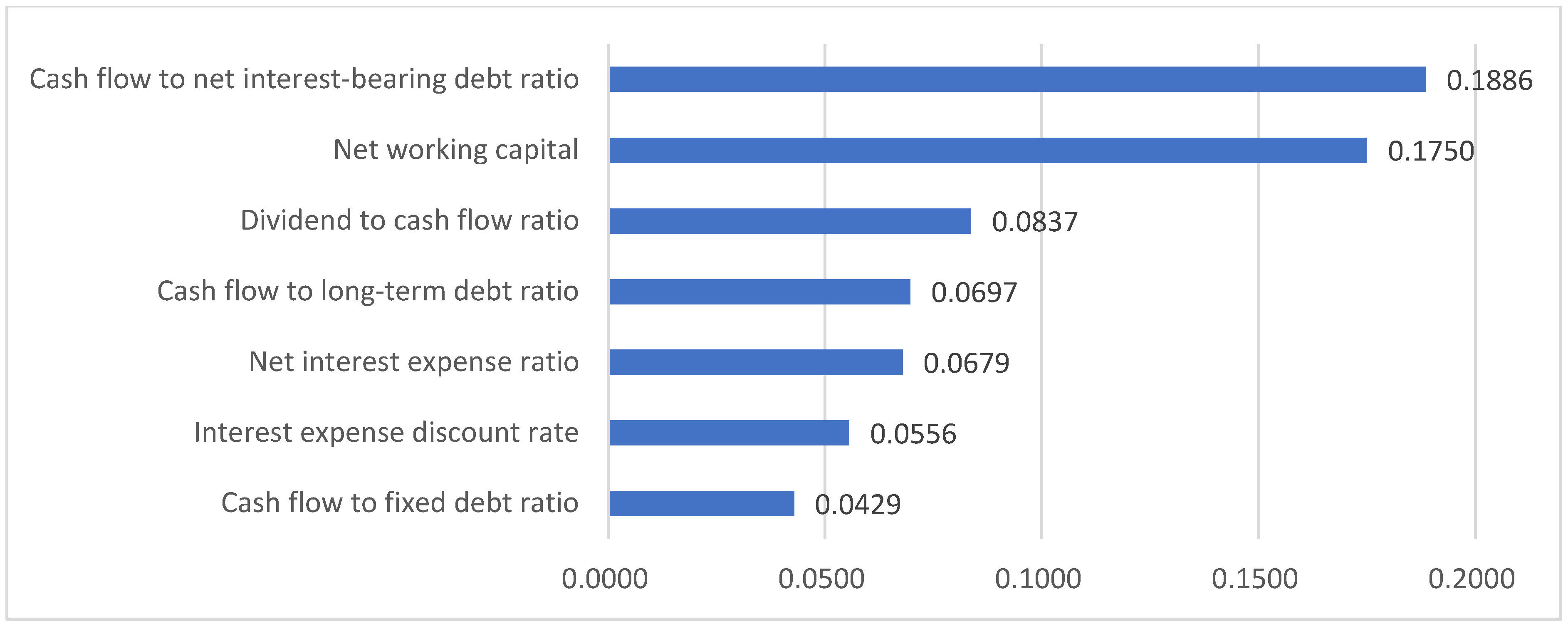
Figure 2.
LightGBM feature importance scores for 173 features under SMOTE-ENN resampling using the financial dataset for the electrical equipment industry.
Figure 2.
LightGBM feature importance scores for 173 features under SMOTE-ENN resampling using the financial dataset for the electrical equipment industry.
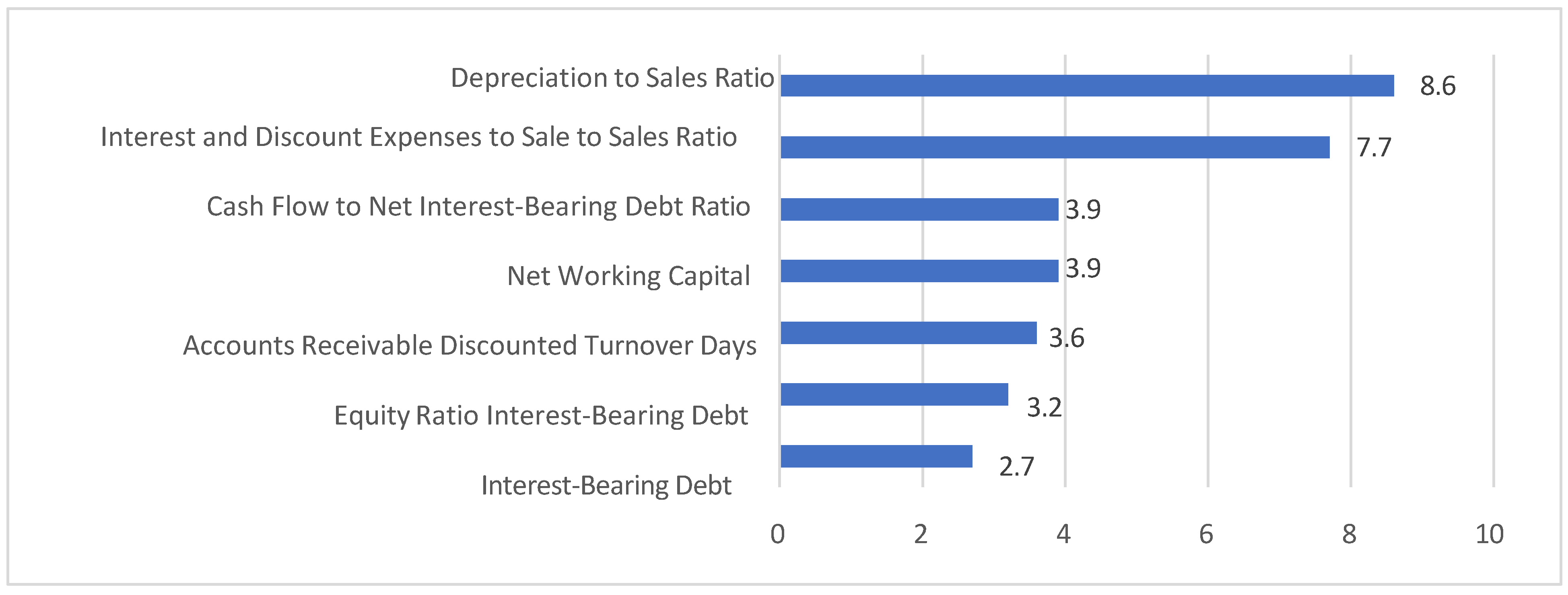
Figure 3.
Workflow of wrapper-based feature selection (Steps 1–4).
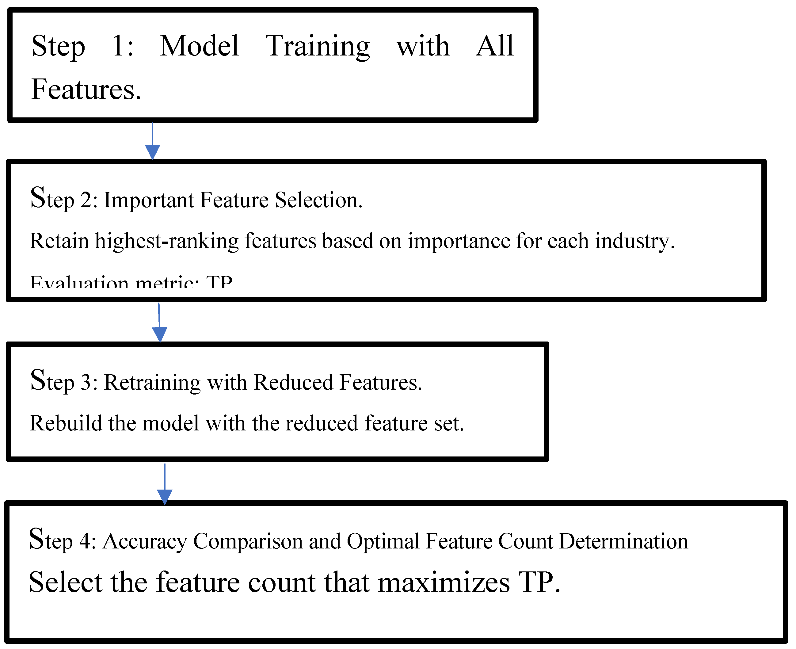
Figure 4.
Importance scores for the top seven features under SMOTE-ENN resampling using the financial dataset for the electrical equipment industry.
Figure 4.
Importance scores for the top seven features under SMOTE-ENN resampling using the financial dataset for the electrical equipment industry.
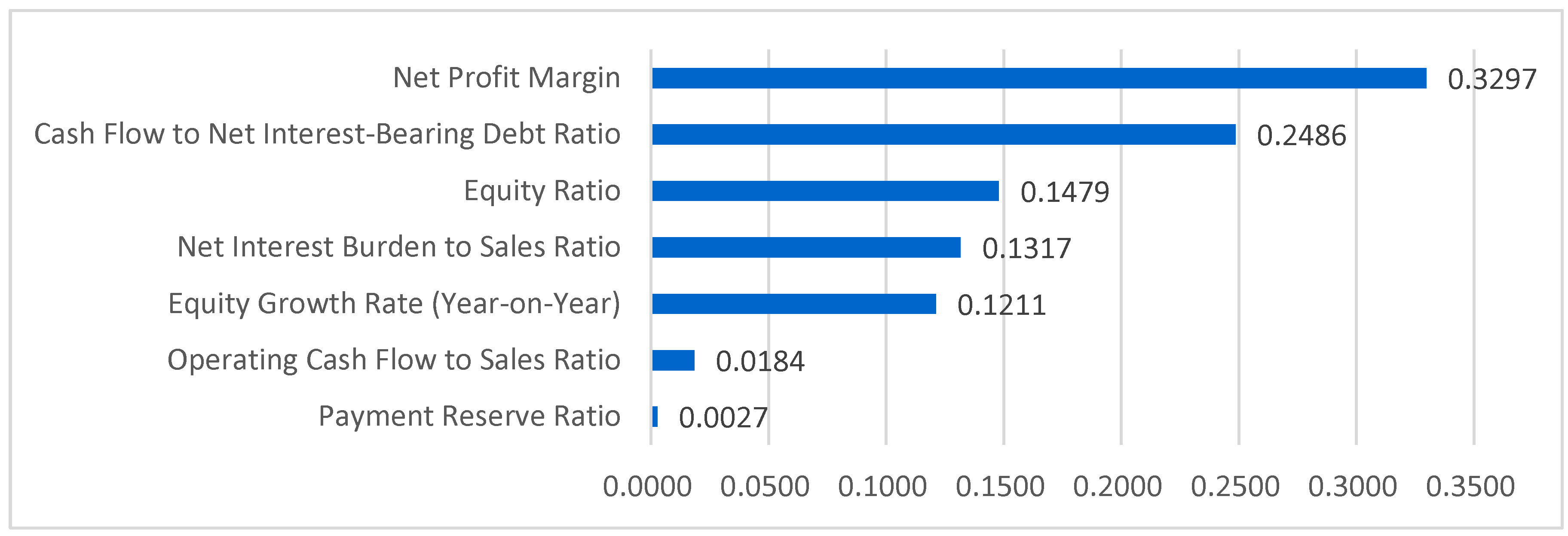
Figure 5.
Importance scores for the top seven features under SMOTE-ENN resampling using the financial dataset for the electrical equipment industry.
Figure 5.
Importance scores for the top seven features under SMOTE-ENN resampling using the financial dataset for the electrical equipment industry.
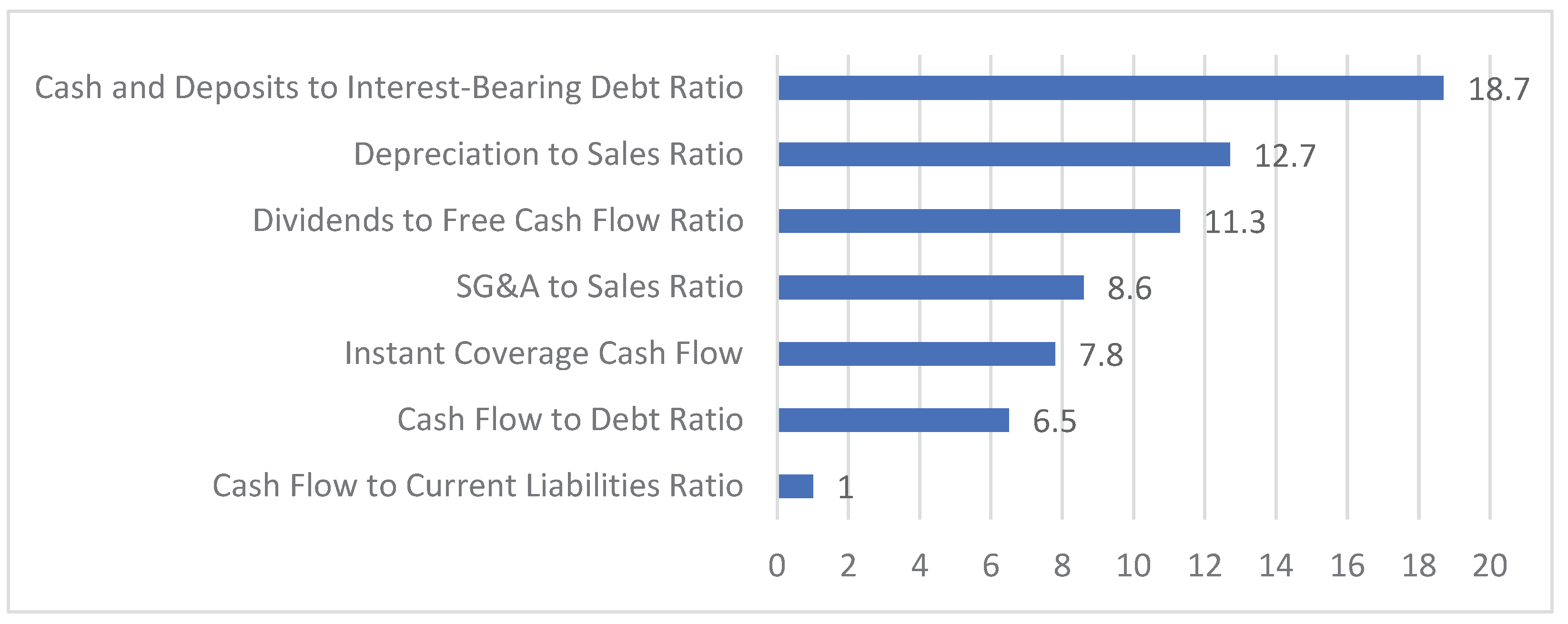
Table 1.
Datasets.
| Industry | Financial | Investment-financing | Comparison | ||||||
|---|---|---|---|---|---|---|---|---|---|
| Bankrupt | Non-bankrupt | Total | Bankrupt | Non-bankrupt | Total | Bankrupt | Non-bankrupt | Total | |
| Construction | 42 | 6,280 | 6,322 | 25 | 3,848 | 3,873 | 25 | 3,848 | 3,873 |
| Real estate | 34 | 3,603 | 3,637 | 21 | 2,089 | 2,110 | 21 | 2,089 | 2,110 |
| Service | 25 | 11,445 | 11,470 | 5 | 4,480 | 4,485 | 5 | 4,480 | 4,485 |
| Retail | 23 | 11,531 | 11,554 | 10 | 5,808 | 5,818 | 10 | 5,808 | 5,818 |
| Electrical equipment | 23 | 9,043 | 9,066 | 11 | 4,722 | 4,733 | 11 | 4,722 | 4,733 |
| Wholesale | 16 | 10,935 | 10,951 | 5 | 5,650 | 5,655 | 5 | 5,650 | 5,655 |
| Total | 163 | 52,787 | 52,950 | 77 | 26,597 | 26,674 | 77 | 26,597 | 26,674 |
Table 2.
Financial indicators and features.
| Classification of financial indicators | Number of features | Examples of features |
|---|---|---|
| Profitability | 47 | Profit margin |
| Return on capital | 15 | Return on assets |
| Margin related | 10 | EBIT 1 margin |
| Productivity | 6 | Revenue per employee |
| Safety | 35 | Equity ratio |
| Growth | 15 | Revenue growth rate (YOY 2) |
| Cash flow | 33 | Cash flow to net debt ratio |
1 EBIT: earnings before interest and taxes. 2 YOY: years.
Table 3.
Hardware and software specifications.
| Hardware/Software | Specification |
|---|---|
| CPU 1 | Core i9-10885H |
| RAM 2 | 32.0 GB4 |
| OS 3 | Windows 11 Pro |
| Programming Language | Python 3.9.7 |
| Machine Learning Package | scikit-learn |
| Parameter Optimization Package | Optuna |
1 CPU, central processing unit. 2 RAM, random-access memory. 3 OS, operating system. 4 GB, gigabytes.
Table 4.
Random Forest true positive count by dataset configuration.
| Actual | Predicted | |||
|---|---|---|---|---|
| Total | Financial | Investment-financing | Comparison | |
| 951 | 478 | 284 | 97 | 97 |
Table 5.
Random Forest true positive count by resampling method and dataset configuration.
| Resampling | Actual | Predicted | |||
|---|---|---|---|---|---|
| Total | Financial | Investment-financing | Comparison | ||
| SMOTE | 317 | 115 | 74 | 19 | 22 |
| SMOTE-ENN | 317 | 177 | 100 | 40 | 37 |
| Kmeans | 317 | 186 | 110 | 38 | 38 |
| Total | 951 | 478 | 284 | 97 | 97 |
Table 6.
Random Forest true positive count by industry and dataset configuration.
| Industry | Total | Financial | Investment-financing | Comparison | ||||||||
|---|---|---|---|---|---|---|---|---|---|---|---|---|
| Actual | Predicted | Recall | Actual | Predicted | Recall | Actual | Predicted | Recall | Actual | Predicted | Recall | |
| Construction | 276 | 152 | 55.07 | 126 | 75 | 59.52 | 75 | 37 | 49.33 | 75 | 40 | 53.33 |
| Real estate | 228 | 133 | 58.33 | 102 | 69 | 67.65 | 63 | 31 | 49.21 | 63 | 33 | 52.38 |
| Service | 105 | 55 | 52.38 | 75 | 50 | 66.67 | 15 | 3 | 20.0 | 15 | 2 | 13.33 |
| Retail | 129 | 58 | 44.96 | 69 | 39 | 56.52 | 30 | 10 | 33.3 | 30 | 9 | 30.00 |
| Electrical equipment | 135 | 59 | 43.70 | 69 | 31 | 44.93 | 33 | 15 | 45.45 | 33 | 13 | 39.39 |
| Wholesale | 78 | 21 | 26.92 | 48 | 20 | 41.67 | 15 | 1 | 6.67 | 15 | 0 | 0.00 |
| Total | 951 | 478 | 50.26 | 317 | 284 | 89.59 | 317 | 97 | 30.6 | 317 | 97 | 30.60 |
Table 7.
Random Forest true positive count and recall rate by resampling method and industry.
| Industry | Total | SMOTE | SMOTE-ENN | K-means | ||||||||
|---|---|---|---|---|---|---|---|---|---|---|---|---|
| Actual | Predicted | Recall | Actual | Predicted | Recall | Actual | Predicted | Recall | Actual | Predicted | Recall | |
| Construction | 276 | 152 | 55.07 | 92 | 35 | 39.13 | 92 | 57 | 61.96 | 92 | 59 | 64.13 |
| Real estate | 228 | 133 | 58.33 | 76 | 37 | 48.68 | 76 | 50 | 65.79 | 76 | 46 | 60.53 |
| Service | 105 | 55 | 52.38 | 35 | 15 | 42.86 | 35 | 18 | 51.43 | 35 | 22 | 62.86 |
| Retail | 129 | 58 | 44.96 | 43 | 9 | 20.93 | 43 | 24 | 55.81 | 43 | 25 | 58.14 |
| Electrical equipment | 135 | 59 | 43.70 | 45 | 15 | 33.33 | 45 | 20 | 44.44 | 45 | 24 | 53.33 |
| Wholesale | 78 | 21 | 26.92 | 26 | 3 | 11.54 | 26 | 8 | 30.77 | 26 | 10 | 38.46 |
| Total | 951 | 478 | 50.26 | 317 | 115 | 36.28 | 317 | 177 | 55.84 | 317 | 186 | 58.68 |
Table 8.
LightGBM true positive count by dataset configuration.
| Actual | Predicted | |||
|---|---|---|---|---|
| Total | Financial | Investment-financing | Comparison | |
| 951 | 420 | 264 | 58 | 97 |
Table 9.
LightGBM true positive count by resampling method and dataset configuration.
| Resampling | Actual | Predicted | ||||
|---|---|---|---|---|---|---|
| Total | Financial | Investment-financing | Comparison | |||
| SMOTE | 317 | 141 | 85 | 21 | 35 | |
| SMOTE-ENN | 317 | 149 | 98 | 22 | 29 | |
| K-means | 317 | 129 | 81 | 15 | 33 | |
| Total | 951 | 420 | 264 | 58 | 97 | |
Table 10.
LightGBM true positive count and recall rate by industry and dataset configuration.
| Industry | Total | Financial | Investment-financing | Comparison | ||||||||
|---|---|---|---|---|---|---|---|---|---|---|---|---|
| Actual | Predicted | Recall | Actual | Predicted | Recall | Actual | Predicted | Recall | Actual | Predicted | Recall | |
| Construction | 105 | 61 | 58.10 | 75 | 47 | 62.70 | 15 | 6 | 40.00 | 15 | 8 | 53.17 |
| Real estate | 228 | 139 | 60.96 | 102 | 62 | 60.78 | 63 | 36 | 57.14 | 63 | 41 | 65.69 |
| Service | 78 | 34 | 43.95 | 48 | 24 | 49.28 | 15 | 2 | 10.00 | 15 | 9 | 60.87 |
| Retail | 129 | 59 | 45.67 | 69 | 47 | 68.00 | 30 | 8 | 26.67 | 30 | 4 | 13.33 |
| Electrical equipment | 276 | 67 | 24.30 | 126 | 50 | 39.58 | 75 | 0 | 0.00 | 75 | 17 | 22.92 |
| Wholesale | 135 | 59 | 43.86 | 69 | 35 | 50.72 | 33 | 7 | 21.21 | 33 | 17 | 52.17 |
| Total | 951 | 420 | 44.15 | 489 | 264 | 54.08 | 231 | 58 | 25.32 | 231 | 97 | 41.95 |
Table 11.
LightGBM true positive count and recall rate by resampling method and industry.
| Industry | Total | SMOTE | SMOTE-ENN | K-means | ||||||||
|---|---|---|---|---|---|---|---|---|---|---|---|---|
| Actual | Predicted | Recall | Actual | Predicted | Recall | Actual | Predicted | Recall | Actual | Predicted | Recall | |
| Construction | 105 | 61 | 58.10 | 35 | 19 | 54.29 | 35 | 21 | 60.00 | 35 | 21 | 60.00 |
| Real estate | 228 | 139 | 60.96 | 76 | 47 | 61.84 | 76 | 49 | 64.47 | 76 | 44 | 57.89 |
| Service | 78 | 34 | 43.95 | 26 | 12 | 46.15 | 26 | 11 | 42.31 | 26 | 11 | 42.31 |
| Retail | 129 | 59 | 45.67 | 43 | 21 | 48.83 | 43 | 22 | 51.16 | 43 | 17 | 39.53 |
| Electrical equipment | 276 | 67 | 24.30 | 92 | 24 | 26.09 | 92 | 28 | 30.43 | 92 | 15 | 16.30 |
| Wholesale | 135 | 59 | 43.86 | 45 | 19 | 42.22 | 45 | 19 | 42.22 | 45 | 21 | 46.67 |
| Total | 951 | 420 | 44.15 | 317 | 141 | 44.48 | 317 | 149 | 47.00 | 317 | 129 | 40.69 |
Table 12.
Changes in true positive count by feature count.
| Features | 4 | 5 | 7 | 15 | 130 | 161 |
|---|---|---|---|---|---|---|
| TP | 559 | 560 | 566 | 529 | 504 | 483 |
Table 13.
Random Forest true positive counts by dataset configuration.
| Actual | Predicted | |||
|---|---|---|---|---|
| Total | Financial | Investment-financing | Comparison | |
| 951 | 566 | 303 | 142 | 121 |
Table 14.
Random Forest true positive counts by resampling method and dataset configuration.
| Resampling | Actual | Predicted | ||||
|---|---|---|---|---|---|---|
| Total | Financial | Investment-financing | Comparison | |||
| SMOTE | 317 | 149 | 84 | 34 | 31 | |
| SMOTE-ENN | 317 | 211 | 113 | 52 | 46 | |
| K-means | 317 | 206 | 106 | 56 | 44 | |
| Total | 951 | 566 | 303 | 142 | 121 | |
Table 15.
Random Forest true positive count and recall rate by industry and dataset configuration.
| Industry | Total | Financial | Investment-financing | Comparison | ||||||||
|---|---|---|---|---|---|---|---|---|---|---|---|---|
| Actual | Predicted | Recall | Actual | Predicted | Recall | Actual | Predicted | Recall | Actual | Predicted | Recall | |
| Construction | 276 | 172 | 62.32 | 126 | 87 | 69.05 | 75 | 44 | 58.67 | 75 | 41 | 54.67 |
| Real estate | 228 | 157 | 68.86 | 102 | 71 | 69.61 | 63 | 43 | 68.25 | 63 | 43 | 68.25 |
| Service | 105 | 57 | 54.29 | 75 | 52 | 69.33 | 15 | 3 | 20.00 | 15 | 2 | 13.33 |
| Retail | 129 | 71 | 55.04 | 69 | 45 | 65.22 | 30 | 14 | 46.67 | 30 | 12 | 40.00 |
| Electrical equipment | 276 | 61 | 62.32 | 126 | 18 | 69.05 | 75 | 29 | 58.67 | 75 | 14 | 54.67 |
| Wholesale | 78 | 48 | 61.54 | 48 | 30 | 62.50 | 50 | 9 | 60.00 | 15 | 9 | 60.00 |
| Total | 951 | 566 | 59.52 | 489 | 303 | 61.96 | 231 | 142 | 61.47 | 231 | 121 | 52.38 |
Table 16.
Random Forest true positive count and recall rate by resampling method and industry.
| Industry | Total | SMOTE | SMOTE-ENN | K-means | ||||||||
|---|---|---|---|---|---|---|---|---|---|---|---|---|
| Actual | Predicted | Recall | Actual | Predicted | Recall | Actual | Predicted | Recall | Actual | Predicted | Recall | |
| Construction | 276 | 172 | 62.32 | 92 | 43 | 46.74 | 92 | 67 | 72.83 | 92 | 62 | 67.39 |
| Real estate | 228 | 157 | 68.86 | 76 | 46 | 60.53 | 76 | 60 | 78.95 | 76 | 51 | 67.11 |
| Service | 105 | 57 | 54.29 | 35 | 16 | 45.71 | 35 | 21 | 60.00 | 35 | 20 | 57.14 |
| Retail | 129 | 71 | 55.04 | 43 | 18 | 41.86 | 43 | 26 | 60.47 | 43 | 27 | 62.79 |
| Electrical equipment | 135 | 61 | 45.19 | 45 | 14 | 31.11 | 45 | 20 | 44.44 | 45 | 27 | 60.00 |
| Wholesale | 78 | 48 | 61.54 | 26 | 12 | 46.15 | 26 | 17 | 65.38 | 26 | 19 | 73.08 |
| Total | 951 | 566 | 59.52 | 317 | 149 | 47.00 | 317 | 211 | 66.56 | 317 | 206 | 64.98 |
Table 17.
Comparison of the top seven features identified by Random Forest from the full set with the seven features selected for the optimized model.
Table 17.
Comparison of the top seven features identified by Random Forest from the full set with the seven features selected for the optimized model.
| 173 Features | 7 Features |
|---|---|
| Cash Flow to Net Interest-Bearing Debt Ratio | Net Profit Margin |
| Net Working Capital | Cash Flow to Net Interest-Bearing Debt Ratio |
| Dividends to Cash Flow Ratio | Equity Ratio |
| Cash Flow to Long-Term Debt Ratio | Net Interest Burden to Sales Ratio |
| Net Interest Burden to Sales Ratio | Equity Growth Rate (Year-on-Year) |
| Interest and Discount Expenses to Sales Ratio | Operating Cash Flow to Sales Ratio |
| Cash Flow to Fixed Liabilities Ratio | Payment Reserve Ratio |
Table 18.
LightGBM true positive count by dataset configuration.
| Actual | Predicted | ||||
|---|---|---|---|---|---|
| Total | Financial | Investment-financing | Comparison | ||
| 951 | 451 | 283 | 87 | 81 | |
Table 20.
LightGBM true positive count by industry and dataset configuration.
| Industry | Total | Financial | Investment-financing | Comparison | ||||||||
|---|---|---|---|---|---|---|---|---|---|---|---|---|
| Actual | Predicted | Recall | Actual | Predicted | Recall | Actual | Predicted | Recall | Actual | Predicted | Recall | |
| Construction | 105 | 72 | 68.57 | 75 | 53 | 72.60 | 15 | 10 | 66.67 | 15 | 9 | 60.00 |
| Real estate | 228 | 138 | 60.53 | 102 | 72 | 70.59 | 63 | 34 | 53.97 | 63 | 32 | 50.79 |
| Service | 78 | 42 | 53.85 | 48 | 32 | 66.67 | 15 | 5 | 33.33 | 15 | 5 | 33.33 |
| Retail | 129 | 44 | 34.11 | 69 | 34 | 49.28 | 30 | 2 | 6.67 | 30 | 8 | 26.67 |
| Electrical equipment | 276 | 93 | 33.70 | 126 | 53 | 42.06 | 75 | 25 | 33.33 | 75 | 15 | 20.00 |
| Wholesale | 135 | 62 | 45.93 | 69 | 37 | 53.62 | 33 | 12 | 36.36 | 33 | 13 | 39.39 |
| Total | 951 | 451 | 47.42 | 489 | 281 | 57.46 | 231 | 88 | 38.10 | 231 | 82 | 35.50 |
Table 21.
LightGBM true positive count and recall rate by resampling method and industry.
| Industry | Total | SMOTE | SMOTE -ENN | K-means | ||||||||
|---|---|---|---|---|---|---|---|---|---|---|---|---|
| Actual | Predicted | Recall | Actual | Predicted | Recall | Actual | Predicted | Recall | Actual | Predicted | Recall | |
| Construction | 105 | 72 | 68.57 | 35 | 28 | 80.00 | 35 | 28 | 80.00 | 35 | 17 | 48.57 |
| Real estate | 228 | 138 | 60.53 | 76 | 59 | 77.63 | 76 | 60 | 78.95 | 76 | 19 | 25.00 |
| Service | 78 | 43 | 55.13 | 26 | 15 | 57.69 | 26 | 16 | 61.65 | 26 | 2 | 7.69 |
| Retail | 129 | 43 | 33.33 | 43 | 19 | 44.19 | 43 | 22 | 51.16 | 43 | 3 | 6.98 |
| Electrical equipment | 276 | 93 | 33.70 | 92 | 54 | 58.70 | 92 | 39 | 42.39 | 92 | 0 | 0.00 |
| Wholesale | 135 | 62 | 45.93 | 45 | 25 | 55.56 | 45 | 27 | 60.00 | 45 | 10 | 22.22 |
| Total | 951 | 451 | 47.42 | 317 | 199 | 62.78 | 317 | 191 | 60.25 | 317 | 61 | 19.24 |
Table 22.
Comparison of the top seven features identified by LightGBM from the full set with the seven features selected for the optimized model.
Table 22.
Comparison of the top seven features identified by LightGBM from the full set with the seven features selected for the optimized model.
| 173 Features | 7 Features |
|---|---|
| Depreciation to Sales Ratio | Cash and Deposits to Interest-Bearing Debt Ratio |
| Interest and Discount Expenses to Sales Ratio | Depreciation to Sales Ratio |
| Net Working Capital | Dividends to Free Cash Flow Ratio |
| Cash Flow to Net Interest-Bearing Debt Ratio | SG&A to Sales Ratio |
| Accounts Receivable Discounted Turnover Days | Instant Coverage Cash Flow |
| Equity Ratio | Cash Flow to Debt Ratio |
| Interest-Bearing Debt | Cash Flow to Current Liabilities Ratio |
Disclaimer/Publisher’s Note: The statements, opinions and data contained in all publications are solely those of the individual author(s) and contributor(s) and not of MDPI and/or the editor(s). MDPI and/or the editor(s) disclaim responsibility for any injury to people or property resulting from any ideas, methods, instructions or products referred to in the content. |
© 2025 by the authors. Licensee MDPI, Basel, Switzerland. This article is an open access article distributed under the terms and conditions of the Creative Commons Attribution (CC BY) license (http://creativecommons.org/licenses/by/4.0/).
Copyright: This open access article is published under a Creative Commons CC BY 4.0 license, which permit the free download, distribution, and reuse, provided that the author and preprint are cited in any reuse.


