
Submitted:
16 October 2025
Posted:
29 October 2025
You are already at the latest version
Abstract
A thermodynamic and quantum derivation of the vacuum energy density uΛ=Λc4/(8πG) is presented from first principles, resolving the long-standing vacuum catastrophe without recourse to Planck-scale physics. Using the Bekenstein–Hawking entropy and Gibbons–Hawking temperature of the de Sitter horizon, we apply E=TS to show that uΛ arises naturally as a maximum entropy bound of the universe. An independent derivation from zero-point energy follows by introducing a physically motivated cutoff at the Lambda scale LΛ=(ℏG/Λc3)1/4, a new quantum–thermodynamic scale defined by G,ℏ,c, and Λ. The resulting Λ-units are unique: vacuum-matching to de Sitter horizon thermodynamics fixes the remaining affine freedom in the dimensional analysis. In this gauge, c and ℏ take unit value, while G and Λ appear symmetrically with their hierarchy encoded by the dimensionless gravitational fine-structure constant αΛ≡c3/(GℏΛ). This unifies thermodynamic and quantum perspectives, eliminating the 10120–fold discrepancy in vacuum energy predictions. We validate the framework across diverse domains—including the Casimir effect, boson and fermion gases, and electromagnetic radiation—each saturating at the same vacuum bound. The results support the Law of Entropic Constraint, in which gravity, inertia and electromagnetism are subject to horizon-encoded information limits. The Planck scale is revealed as incomplete without the inclusion of Λ. The Λ system of units emerges as its natural completion—superseding the Planck scale, just as Planck units superseded Stoney’s once ℏ was recognized as fundamental.
Keywords:
cosmological constant problem
; dark energy
; Bekenstein–Hawking entropy
; de Sitter spacetime
; Gibbons–Hawking temperature
; gravitational fine-structure constant
; Casimir effect
; horizon thermodynamics
; natural units
; vacuum energy density
; zero-point energy
1. Introduction
The cosmological constant has undergone a remarkable transformation. Introduced by Einstein to stabilize the universe and later abandoned, it has returned as a cornerstone of modern cosmology with the discovery of accelerated expansion [1,2,3]. Yet its physical meaning remains obscure [4]. The “vacuum catastrophe”— quantum field theory’s (QFT) estimate of a vacuum energy density exceeding cosmological bounds by —reveals a deep gap in how quantum mechanics, gravity, and thermodynamics interrelate.
Thermodynamic treatments of spacetime (e.g., Jacobson [5], Verlinde [6], Padmanabhan [7]) suggest that horizon entropy and temperature encode gravitational dynamics, but they do not pin down the observed vacuum density nor the role of as a fundamental constant. If is fundamental, physics must explain why it fixes the vacuum energy and how it enters the basic scales of nature [8,9]. This paper makes four contributions:
-
Thermodynamic Derivation of the Vacuum Energy.Using the Gibbons–Hawking temperature of the de Sitter horizon [10], the Bekenstein–Hawking entropy [11,12], and the Clausius relation (or ) [5,13], we obtain directly the vacuum energy density in general relativity (GR),identifying as a finite entropy bound of the universe (throughout, u denotes a generic energy density)[10,14,15].
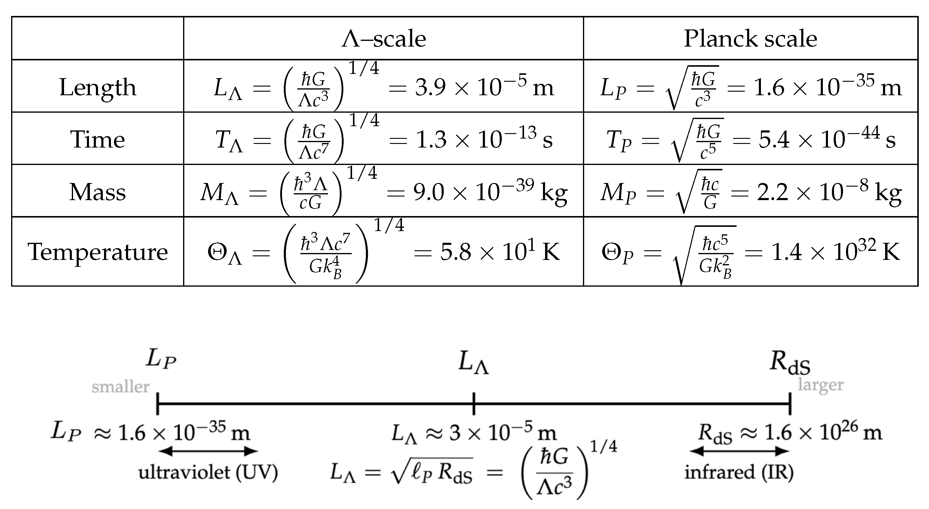
- A New Quantum Scale—the -Scale. As represents a finite information capacity of the universe, we argue the Planck scale is incomplete without it [16]. Combining selects a unique scale (Figure 1.) We introduce the dimensionless gravitational fine-structure constant (GFSC),an entropic bound that anchors quantum theory to cosmology and resolves the vacuum catastrophe without invoking Planck-scale physics. Details and the dimensional analysis are given in Appendix A. For historical context see Appendix B.
-
Cross-Domain Validation of the -scale.
- A Quantum Derivation of from the Zero-Point Energy (ZPE): Crucially, we also provide an explicit zero-point (ZPE) density-of-states derivation of in Eq.(1), based on the -scale in Figure 1 (see Section 8 and Appendix C), not via boson/fermion cancellations but through a finite mode budget. Without Planck-cutoff assumptions, ultraviolet divergences are eliminated, yielding a finite and radiatively stable vacuum energy [4,17].
2. Deriving the Vacuum Energy from Horizon Thermodynamics
2.1. Thermodynamics of Causal Event Horizons
The thermodynamic structure of causal event horizons — a defining feature of GR, partitions spacetime into accessible and inaccessible regions. This division gives rise to observable thermodynamic properties: temperature, entropy, and energy. The universality of their expressions and the deeper thermodynamic structure are governed by the four laws of black hole thermodynamics [11,12,18]. See Figure 2.
This viewpoint has been developed by many authors over the past decades [5,6,7,10,11,12,18,20]. The three archetypal cases are shown schematically in Figure 3, Figure 4, Figure 5 and Figure 6.
An accelerated observer in flat spacetime perceives a Rindler horizon and detects a thermal bath at the Unruh temperature [20]. See Figure 3.
A black hole horizon radiates at the Hawking temperature, its entropy fixed by the Bekenstein–Hawking area law [11,12] See Figure 4 and Figure 5.
Finally, de Sitter spacetime, relevant to our universe with positive , possesses a cosmological horizon with Gibbons–Hawking temperature and entropy proportional to its area [10]. See Figure 6.
This principle - that causal event horizons are inextricably tied to an entropy and temperature - holds irrespective of the horizon’s origin — whether due to acceleration, mass, or vacuum energy — and it is the universality of this horizon thermodynamics that forms the basis for our derivation of the vacuum energy density. The common structure across these three spacetimes is illustrated in Table 1.
Because our universe is asymptotically approaching de Sitter space, its horizon provides the correct setting to apply the identity , yielding a finite and universal expression for the vacuum energy density in the context of horizon thermodynamics [19,21,22], and consistent with quantum–informational perspectives [23].
2.2. Deriving the Vacuum Energy from Horizon Thermodynamics
The integrated form of the First Law of Thermodynamics , has its deeper roots in the Second Law of Thermodynamics, formalized by Rudolf Clausius in the mid-19th century [13,24],
We now make use of the thermodynamic identity, applied to the cosmological horizon of de Sitter spacetime.
2.3. Horizon Energy E
To obtain the total energy content E of the de Sitter universe, we begin with the entropy S of the de Sitter horizon:
Substituting the de Sitter radius into this expression:
Note that Eq.(6) has the GFSC defined in Eq. (2) embedded within it, making this a maximum bound on entropy. Next, we use the Gibbons–Hawking temperature:
Combining:
2.4. Horizon Volume and Energy Density
The spatial volume enclosed by the de Sitter horizon is:
The vacuum energy density is then:
Simplifying:
This elegant result is deeply significant. In GR Eq. (11) emerges only from dimensional consistency of the Einstein field equations, here the observed vacuum energy density is derived without invoking any matter fields or action principles. Instead, it arises from applying thermodynamics to the geometry of de Sitter spacetime.
3. From Thermodynamics to a New Quantum Scale in Nature
QFT has not yet produced a reliable prediction of the observed vacuum energy density when regulated at Planck scales because it is constructed without reference to . Being blind to the large-scale curvature of spacetime, it is a miscalibrated scale. A new quantum scale is therefore needed, one that includes ab initio. Only then can we meaningfully measure the vacuum without triggering a theoretical breakdown [7].
Our thermodynamic derivation of fixes the vacuum energy density as a finite, horizon–regulated quantity. It is this that justifies why should be treated not as an arbitrary parameter but as a fundamental constant of nature, on the same footing as c and ℏ. Each of these constants encodes a fundamental limiting principle: c defines the maximum velocity of causal signals, ℏ defines the minimum quantum of action, and defines the maximum entropy – the finite information capacity of the universe. [10,11,12].
A dimensional analysis involving yields a new set of natural units in Appendix A, illustrated in Figure 1 and applied in Figure 7. For historical context see Appendix C.
This new quantum scale, unlike the Planck scale, avoids the break down when measuring the quantum vacuum. It signifies a new unity between GR, QFT and thermodynamics, in which the vacuum catastrophe is revealed as illusory, and nothing more than a physicist’s ghost. see Figure 7.
4. Forces in -Units: How Interactions Respect the Entropy Bound
Within the -framework, horizons defined by impose a finite entropy bound on spacetime (see Section 2.1); deviations from geodesic motion couple to this structure, producing an entropic response. Expressed in -units, inertial , gravitational and electromagnetic forces , reduce to the scales shown in Figure 8:
We see that is present in all the force terms (Figure 8) and that Newton’s constant G, drops out of the expression for the gravitational force term, leaving a ’gravitational force’ without any need for G,
One finds from the definition of the GFSC in Eq. (2),
substituting Eq. (13) into the inertial force term we find,
Thus inertial forces share the same form as gravitational ones but scaled by a factor . It is remarkable that the electromagnetic sector (a gauge interaction) respects the same entropic bound, taking just a fraction, , of the inertial force.
Gravity looks weak at macroscales because the gravitational unit is suppressed relative to by , while gauge forces scale with their own dimensionless couplings (e.g. ). In all cases the common thread is that all forces and their resulting motions are constrained by a finite-information capacity of the vacuum.
5. Electromagnetic Radiation and the Vacuum Bound
Electromagnetism, like inertia and gravity, is constrained by the vacuum’s entropy bound. In -units, the Coulomb force [25] is revealed not as arbitrarily strong but as a fraction of the vacuum’s maximal force, scaled by the fine-structure constant . This reframes electromagnetic interactions as vacuum-limited couplings.
Gauge invariance still permits shifting the zero of potential, but the -framework fixes the maximum field strength by horizon thermodynamics. Thus, electromagnetism joins inertia and gravity as an expression of the same entropic constraint.
To illustrate this explicitly, we derive the Poynting flux [26,27] in -units, showing how energy transport in electromagnetic waves saturates at the same thermodynamic limit set by . See Table 2.
5.1. The Poynting Flux in -Units
In standard notation the time–averaged Poynting flux for a plane electromagnetic wave in vacuum is
The corresponding flux has a magnitude given by:
Expressing using the fine-structure constant [29]:
So:
The average radiative flux is thus:
This is a striking result. It shows that the classical electromagnetic flux density is directly proportional to the vacuum energy density of spacetime — scaled by the fine-structure constant, a quantum measure of the coupling strength of light to matter.
Our Poynting analysis reveals the EM energy/flux, a gauge field, respects the bound set by .
6. The Casimir Effect and the Quantum Vacuum
The Casimir force between conducting plates has long been taken as evidence of vacuum fluctuations arising from a modified mode spectrum between the plates [30,31]. However, the precise connection between such boundary–dependent zero-point energies and the homogeneous cosmological vacuum remains an open question in contemporary physics [4,32,33].
The standard expression for the pressure is,
where d is the plate separation. The minus sign denotes vacuum tension (negative pressure): suppressed modes between the plates make the interior zero-point pressure lower than outside, producing an inward force. This fixes the sign (tension) of the vacuum in a bounded geometry. See Figure 9.
Introducing the -length cutoff
and substituting into Eq.(24), shows that the Casimir pressure is a fixed fraction of the vacuum bound,
Thus a laboratory-scale quantum effect validates the same vacuum limit that emerges thermodynamically from de Sitter horizons. It is precisely a negative pressure that gravitates in GR, yielding a cosmic repulsion and an accelerated universal expansion. See Figure 10.
6.1. From Quantum Fluctuations to Measurable Force
The length sits in the Casimir window. With CODATA values,
which lies squarely in the mid–IR/THz, precisely the range where Casimir forces have been probed (e.g. Lamoreaux’s torsion–pendulum and subsequent torsional studies [31,34]). This coincidence is not incidental in our framework.
Evaluating the ideal () plate–plate pressure at the length yields a quartic correspondence with the GR vacuum density. This suggests, in principle, a laboratory route to infer using real materials, with corrections incorporated through the standard Lifshitz framework [35]. Figure 11 and Figure 12 outline how such a determination of could be made experimentally from micron–scale force measurements, far above the Planck length .
6.2. On the Origins of the Casimir Effect
The interpretation of Casimir forces has long been debated: zero–point fluctuations versus retarded van der Waals interactions. The Lifshitz framework [35] shows these are equivalent descriptions, with the Casimir expression emerging as the limiting case of Lifshitz theory for ideal reflectors ().
7. Quantum Gases: Bosons and Fermions in Thermal Equilibrium with the Vacuum
Both bosonic and fermionic gases exhibit the same thermodynamic law: their equilibrium energy densities scale quartically with temperature, [36,37]. This Stefan–Boltzmann scaling reflects a deeper geometric constraint imposed by causal horizons. For massless bosons such as photons, the cosmic microwave background (CMB) energy density is where,
while fermionic gases such as relic neutrinos form the cosmic neutrino background (CB), is denoted by ; denotes the number of light neutrino species (we take ),
Substituting the –temperature,
into the boson and fermion energy densities, reveals both as fixed fractions of the vacuum energy, see Figure 13. Bosons saturate the bound rapidly, while fermions are Pauli-suppressed, but both approach finite values consistent with a capped vacuum.
8. Quantum Derivation of the Vacuum Density (ZPE with a cutoff)
We write the zero–point energy density in the standard (mode–count) form
where for a relativistic linear dispersion . Evaluated with a Planck–scale ultraviolet cutoff this gives
The scale and the physical cutoff
The units fix a natural length, time, and (linear) frequency
Horizon thermodynamics selects a universal numerical factor so that UV saturation occurs at
where and is a pure number fixed by vacuum matching. Using
one gets
The explicit integral with the matched upper limit
Inserting into (29) (with ) gives
Thus the same quartic ZPE integral, evaluated at the cutoff , reproduces exactly the GR vacuum density.
Massive fields decouple at the scale
For a species of mass m with angular frequency ,
and the same , the energy density becomes
with degeneracy s. Hence heavy fields are parametrically suppressed by powers of . At the cutoff ( meV), only effectively massless modes (photons; plausibly gravitons) contribute appreciably.
- Interpretation.
The result above is not a fine–tuned cancellation but a horizon–imposed saturation of the mode count: a finite entropy/energy budget set by . Radiative stability follows naturally—high–frequency loops do not shift [4,5,7,39].
Repeating the calculation with Planck’s () spectrum reproduces
with (equivalently, for ), providing a useful consistency check; see Appendix C.
9. Law of Entropic Constraint (LoEC)
Across horizon thermodynamics, Casimir, quantum gases and EM flux, all ceilings track a single dimensionless constant:
Fixed by horizon matching (Section 2.1, Appendix A), a direct corollary is the vacuum ceiling
The cosmological constant and corresponding are small because the entropy of the universe is so large, bounded by Eq. (38). With Boltzmann’s relation (penned by Planck himself) [40,41],
we have
This is an immensely large entanglement entropy [5], meaning the number of accessible microstates available to the quantum vacuum is truly colossal. The smallness of is therefore a consequence of the largeness of the GFSC, . Furthermore, this finite number of microstates, according to the LoEC, cannot be created or destroyed arbitrarily: the total capacity is conserved [14]. A universe in which removes the bound, , and the -scale would disappear.
Our preceding analysis has shown that seemingly independent domains converge on the same vacuum bound . This unification points to a deeper principle: the vacuum encodes a maximum entropy, and all physical processes respect this limit.
Inertia emerges from entanglement across local Rindler horizons, while gravity reflects curvature-induced entropy bounds in de Sitter space.
If sets the universe’s entropy capacity, models that treat dark energy as a time-varying are in tension with horizon thermodynamics, since would drift unless compensated by entropy production. Likewise, varying c or ℏ would shift the same bound. The Hubble-tension [42,43] is therefore more plausibly traced to measurement systematics or new matter-sector physics than to variations in . Gravity need not be fundamental: the –framework suggests it is the macroscopic imprint of information loss across causal horizons.
| Box 9.1: The Law of Entropic Constraint (LoEC): Summary |
All physical processes are constrained by a maximum entropy determined by the vacuum’s causal structure, underpinned by the dimensionless GFSC.
|
10. Discussion
Einstein’s aesthetic dilemma concerning the cosmological constant has haunted theoretical physics for more than a century. In extending his 1915 field equations [44],
with a cosmological constant [45],
Einstein complained that he had “always had a bad conscience,” finding it “ugly indeed that the field law of gravitation should be composed of two logically independent terms” [46]. His discomfort reflected the sense that had been appended without justification. Yet historical precedent shows this unease was misplaced. Newton had already noted in the Principia that spherical symmetry admits not only the familiar inverse-square force law but also a linear term proportional to R [47]. See Figure 14.
What appeared to Einstein as a blemish was in fact the natural echo of a symmetry already recognised in classical gravity.
The thermodynamic interpretation of general relativity reveals why the cosmological term is inevitable. Jacobson demonstrated that the Einstein equations without are equivalent to the Clausius relation [5], expressing the balance of heat and entropy flow across local horizons.
| Box 10.1: Thermodynamic Bookkeeping ↔ Einstein equation (with ) |
|
Once the cosmological constant is restored, the equations assume the structure of the full first law of thermodynamics,
with the contribution supplying the missing work term. In thermodynamic language, vacuum energy has the unique equation of state , so the cosmological constant precisely mimics the work function of the vacuum. As Padmanabhan [7] emphasised, this endows spacetime with the ability to perform work and completes the thermodynamic analogy. Far from being an arbitrary appendage, is the key to upgrading Jacobson’s Clausius identity into the full first law, closing the circle of the thermodynamic derivation presented in Section 2.2.
Once is recognised as a fundamental constant, a new natural scale inevitably follows. The -length,
Equation (45) shows that is simply the geometric mean scale derived from the Planck length and the de Sitter horizon radius (up to the fixed factor ). This ties together quantum uncertainty, causality, and horizon thermodynamics in a single invariant.
A central point of comparison is with the traditional Planck scale. In Planck units, the vacuum energy density expected from zero-point fluctuations is catastrophically large, exceeding observation by some 120 orders of magnitude. This mismatch makes the observed value of
appear absurdly small [48,49,50]. Yet this impression arises only when Planck units are taken as the measure of naturalness [51]. Once is admitted as a fundamental constant, a new unit system emerges in which is not anomalously tiny but exactly the saturation value set by horizon thermodynamics. The -length provides the correct cutoff, and the resulting vacuum energy is radiatively stable [4,52]. In this framework the Planck scale is revealed as inadequate for “weighing the vacuum,” while the -scale resolves the paradox without fine-tuning. What appears as an inexplicable smallness is reinterpreted as the fundamental benchmark of information capacity. Thus the vacuum catastrophe is not a failure of physics but the signal that the Planck yardstick breaks down when applied to the quantum structure of empty space.
Several further consequences flow directly from treating as fundamental and recognising the -scale as basic:
- Bound on entropy. imposes a universal entropy bound of spacetime. The Law of Entropic Constraint (LoEC) asserts that all physical processes are restricted by this bound, encoded in the de Sitter horizon entropy . The vacuum energy is a necessary corollary of the bound and the GFSC encodes it.
- Finite and stable vacuum energy. The LoEC forbids , since the de Sitter entropy bound would otherwise change in time. Time-varying models (quintessence/phantom) [53,54,55,56] are therefore not a true cosmological constant () and proposals to solve the Hubble tension [57] with contradict both LoEC and the horizon–thermodynamic derivation.
- Quantum derivation of vacuum energy. In -units, the zero-point energy sum saturates at the -scale reproducing the GR vacuum density in Eq.(46), and yielding the radiatively stable derivation that Zel’dovich and Sakharov first sought, unifying the quantum and cosmological vacua as a single entity [17,58].
- Cross-domain consistency. Independent systems all saturate the -bound in the same way. Bosonic and fermionic gases at the -temperature approach fixed fractions of ; Casimir pressures with separation reproduce the vacuum density of GR; electromagnetic fluctuations scale as via the Poynting analysis. These diverse phenomena confirm that the same entropy ceiling governs matter, radiation, and the vacuum alike [30,59,60].
These consequences show that the -framework addresses simultaneously the vacuum catastrophe, the stability of the vacuum, and the constancy of couplings. In each case, the objections that once plagued the cosmological constant dissolve when it is treated as the natural thermodynamic completion of the first law and the basis of a new quantum scale.
In this light, Einstein’s dilemma disappears. The two-term structure that he found unsightly is the unavoidable expression of deeper principles. Just as Newton showed that two distinct force laws are permitted by symmetry, the thermodynamic derivation shows that two terms are demanded by consistency: the Einstein tensor encodes the response of spacetime geometry, while the -term enforces its finite information capacity through the -scale. Einstein’s infamous “blunder” is thereby reinterpreted as an inevitable consequence of symmetry and thermodynamics. Recognising as fundamental not only restores logical unity to the field equations but also reframes them as the complete first law of spacetime dynamics, with the -scale as the bridge between quantum theory and cosmology.
Planck versus scales
The Planck system of units was constructed heuristically by equating a Schwarzschild radius with a Compton wavelength, and has long been assumed to define the natural scale of quantum gravity. Yet this construction is ad hoc and plagued by pathologies. It predicts a vacuum density overshooting observation by (the “vacuum catastrophe”) [4], a runaway instability at every instant [61,62], and a large conceptual gap (“Planck desert”) between and Standard Model scales [63,64]. Most significantly, as highlighted in Table 3, the Planck system is thermodynamically sterile: its base set — is purely mechanical, with introduced only by convention—the base set by contrast, embeds a thermodynamic constant ab initio: fixes the de Sitter entropy bound, so information capacity is intrinsic rather than appended. Its base units follow not from heuristic dimensional analysis but from the Clausius relation , ensuring consistency with the observed vacuum energy density. In this sense, the framework subsumes and supersedes the Planck scale as a complete natural system, unifying quantum, thermodynamic, and gravitational perspectives.
11. Conclusions
The analysis presented suggests, is not a ’blunder’ but the missing piece of the cosmic–quantum jigsaw puzzle [45,46,65]. Its genuine inclusion at the foundations of physics reveals the vacuum not as a place of violent discontinuity, but as a regulated structure where spacetime remains smooth and continuous even at the smallest scales. Far from heralding the breakdown of the laws of physics, the -scale completes them. The supposed realm of quantum gravity, long confined to the Planck scale, is displaced by some thirty orders of magnitude into a domain where thermodynamic and quantum principles converge. Taken together, our results recast from an expendable add-on to a fundamental constant that fixes the universe’s information capacity [14]. The –framework turns the divergent zero-point sum into a finite non-zero value because the de Sitter horizon enforces geometric saturation: only modes that “fit” contribute, while heavy, short-wavelength modes are suppressed [66]. thereby emerges as a thermodynamic necessity, with the maximum entropy
providing the global bound.
In this light, the Law of Entropic Constraint (LoEC), underpinned by the gravitational fine-structure constant
functions as a conservation-like principle: entropy can be redistributed locally through unitary dynamics, but the total number of accessible microstates is bounded globally. This explains why de Sitter spacetime lacks global energy conservation and unitarity, even while local conservation laws remain intact [22,67].
Historically, this framework fulfils what Planck originally sought. His aim was to resolve the UV catastrophe, via an exact law of entropy conservation [68,69]. Instead his journey initiated the quantum revolution. The –framework, by contrast, subsumes and supersedes the Planck system, providing the entropy law he sought through the LOEC.
Most significantly, this perspective resolves Einstein’s misgivings about the “ugly” addition of two terms [46]. It provides the Zel’dovich–Sakharov program [17,58] with a successful, radiatively stable derivation of vacuum energy, and extends Jacobson’s thermodynamic derivation from local Rindler horizons to the full de Sitter horizon [5]. In doing so, the –framework unifies quantum, gravitational, and thermodynamic perspectives.
In the gravitational context, thermodynamic constraints are not merely consequences of geometry; they give rise to it [5,6]. Spacetime’s structure may be the most elegant entropy-management architecture the universe has ever devised, with setting its intrinsic scale and, in the process, revealing gravity’s innate quantum nature.
Author Contributions
Conceptualization, methodology, formal analysis, investigation, visualization, writing—original draft, and writing—review & editing, all by the author.
Funding
The author conducted this research independently and received no external funding.
Institutional Review Board Statement
Not applicable. This theoretical study involved no human or animal subjects.
Informed Consent Statement
Not applicable.
Data Availability Statement
All data supporting the findings of this study are contained within the article and its appendices (and any supplementary materials).
Acknowledgments
The author gratefully acknowledges Dr. John F. Cooper for insightful discussions and constructive comments that improved the manuscript.
Image Credits
Images used in Appendix B are in the public domain and were obtained from institutional collections via Wikimedia Commons. No permissions were required.
Conflicts of Interest
The author declares no conflict of interest.
Use of Artificial Intelligence Tools
Artificial intelligence tools (ChatGPT, OpenAI, 2025) were used to assist in formatting, language refinement, and LaTeX code organization. All scientific content, data analysis, derivations, and interpretations are solely the author’s original work.
Abbreviations
The following abbreviations are used in this manuscript:

Table 4.
Abbreviations used in this manuscript.
| Symbol | Meaning / Definition |
|---|---|
| Cosmological constant (inverse length squared; also sets the entropy/area scale). | |
| Vacuum energy density, . | |
| length, time, mass scales: | |
| –temperature unit: | |
| Planck length, time, mass: , , . | |
| Electromagnetic fine–structure constant, (HEP convention sets , giving ). | |
| Gravitational fine–structure constant, . | |
| GR, QFT | General Relativity; Quantum Field Theory. |
| de Sitter horizon radius; Hubble rate (). | |
| Gibbons–Hawking, Unruh, Hawking temperatures. | |
| Bekenstein–Hawking and de Sitter horizon entropies. | |
| Surface gravity (sets ). | |
| Matched cutoff (linear and angular) frequencies. | |
| ZPE | Zero–point energy. |
| LoEC | Law of Entropic Constraint. |
| PoE | (Einstein’s) Principle of Equivalence. |
| DOS | Density of states. |
| CMB, CNB, | Cosmic Microwave / Neutrino Background; symbols for the photon and neutrino energy densities. |
| Horizon angular velocity; horizon electric potential (work coefficients). | |
| Infinitesimal changes in black–hole angular momentum and electric charge. |
Appendix A. Derivation of the Λ-Scale
We build natural units from by writing any target unit X as a monomial
with exponents to be determined from dimensional balance in base units (cf. Planck’s 1899 dimensional construction; here extended to include [16]):
Hence the dimension of is
The three exponents are exactly the three linear forms that will become the rows of the matrix in the formal derivation.
- Appendix A.0.1 Length LΛ: solve the linear system by inspection.
For a length unit we require , i.e.
Thus the general solution is a one-parameter family
Two instructive choices:
- Appendix A.0.2 Time TΛ: identical logic.
For a time unit we require , hence
So the family is
Two instructive choices:
- Appendix A.0.3 Mass MΛ: again, solving by inspection.
For a mass unit we require , i.e.
Therefore
Two instructive choices:
|
By–inspection solutions (one–parameter families). For the required exponents for the base units are: Two instructive choices. |
The three blocks above are the three row-constraints we shall later collect into the matrix. Solving each target dimension exposes the same one-dimensional affine freedom: dimensional analysis alone leaves a free parameter p (a nullspace direction). In practice, this means there is a whole family of possible “natural units.” Choosing reproduces the Planck units, while yields the -units with their characteristic quarter-powers.
This inspection method already shows that dimensional analysis by itself cannot uniquely fix the scale: the affine parameter simply shifts weight among . To determine which member of the family Nature selects, one must go beyond inspection. [16,70].
Appendix A.1. Deriving and Fixing the Λ-Unit System
To formalize the inspection analysis above, we now write out the dimensional algebra explicitly. Using our four constants are defined in (A2), we consider a monomial
and demand . Matching exponents of gives the linear system
This matrix has rank 3, hence a 1-dimensional nullspace. A basis vector is
Therefore any particular solution can be shifted by for arbitrary :
- Vacuum matching anchor and uniqueness.
Dimensional analysis leaves the affine family (A13). Physics fixes λ by the vacuum–matching postulate (QFT cutoff = GR vacuum):
In exponent space (order ) this requires
so the unique length exponents are
With the kinematic anchors and this yields
Conclusion: with as bases and four constants , every target dimension has a 1-parameter family of exponent quadruples. This is the mathematical origin of the “infinitely many ”.
Appendix A.2. Planck, Stoney, and Λ as “nullspace + anchors”
A unit system becomes unique once we add enough physical anchors to kill the nullspace freedom(s). With the vacuum matching (A14) selecting , the dimensionless values of the constants in -units are summarized in Table A1.
Table A1.
Dimensionless values in -units. Anchors enforce . Vacuum matching selects the symmetric point, yielding and , where is the GFSC.
Table A1.
Dimensionless values in -units. Anchors enforce . Vacuum matching selects the symmetric point, yielding and , where is the GFSC.
| Constant | Base dimensions | in -units | Note |
|---|---|---|---|
| c | 1 | anchor | |
| ℏ | 1 | anchor | |
| G | paired with ; product fixed | ||
| symmetric with |
- Planck units {G, ℏ, c} [16].
Here constants for 3 bases no nullspace. Uniqueness comes for free once we impose the usual identifications and .
- Stoney units {G, c, e} (+ EM convention) [71].
Relativity (), gravity (G), and an electromagnetic normalization (choice of Coulomb constant / rationalization) fix the set. One recovers and a natural charge/action scale (e.g. in SI) by construction.
- Λ-units {G, ℏ, c, Λ}.
Now for 3 bases ⇒one free parameter (the in (A13)). Two standard anchors are kept:
A single -specific anchor removes the remaining freedom:
This fixes the length scale uniquely:
Thus the -triple is unique once (A18) is adopted.
Equivalent algebraic symmetry. For length, write . Solving (A11) for gives the family
Imposing the simple equal-weight symmetry (“give quantum and gravity equal weight, oppose with equal magnitude”) yields
i.e. exactly (A19). This symmetry condition is just the exponent form of the vacuum matching (A18).
Appendix A.3. Why most choices do not return c and ℏ
Because live on the affine line (A31), generic choices give
The anchors (A17) pick out the subfamily consistent with relativity and quantum kinematics; the -anchor (A18) then selects one point on that subfamily—giving (A19). This mirrors explicit counterexamples: other valid exponent choices produce a different velocity scale and a different action scale.
Appendix A.4. Temperature and kB
Historically, Planck [16] introduced a fourth base dimension and used to tie temperature to energy. Two consistent options:
-
With (four bases ). Add . Then a natural -temperature follows from horizon thermodynamics:Up to order-unity factors, this is the de Sitter/Gibbons–Hawking scale.
- Without (modern HEP convention). Set so temperature is measured in energy; is not an independent base dimension and (A19) suffices.
Appendix A.5. Practical “algorithm” (no trial & error)
- Write the dimensional matrix (A11); solve once to get a particular solution and the null vector .
- Enforce the two standard anchors (A17) so that unit speed is c and unit action is ℏ.
- Impose the single -anchor (A18) ⇒ fix the free parameter .
- Read off the exponents for as in (A19); if using , define via (A22).
- Remark on electromagnetism.
is dimensionless and not set by units. One may choose EM conventions (e.g. Heaviside–Lorentz [27,72,73]) so that is absorbed, but the -unit uniqueness rests entirely on the mechanical anchors plus the -postulate, not on EM conventions.
Therefore: Admitting as a fundamental constant introduces one nullspace degree of freedom in the dimensional algebra; a single, physically motivated vacuum-matching postulate removes it and yields a unique -scale. This both explains the infinity of formal solutions and why the physically relevant -triple emerges uniquely.
Table A2.
Comparison of natural unit systems. Enough anchors remove nullspace freedom.
| System | Constants used | Base dims. | Anchors imposed | Unique outcome |
|---|---|---|---|---|
| Stoney (1881) | (with ) | (i) ; (ii) G; (iii) EM normalisation (Coulomb const.) | Recovers and natural charge/action scale ( in SI) | |
| Planck (1899) | (opt. ) | or | (i) ; (ii) ; (opt. iii) for | Unique ; with , Planck temperature |
| -scale (present) | (opt. with ) | (i) ; (ii) ; (iii) | Unique ; with , |
Once are admitted, dimensional analysis alone leaves a one-parameter family of monomials. A single, physically motivated postulate—matching the QFT cutoff to the GR vacuum density—selects a unique member: the -scale. What looks like algebraic freedom is therefore resolved by thermodynamics, which also explains why the physically relevant -triple emerges uniquely.
Appendix A.6. The Λ Scale as a Geometric Mean
An elegant property of the scale is that it lies midway, on a logarithmic scale, between the Planck length and the de Sitter horizon radius . This can be shown directly by inspection. Define the familiar quantities:
Taking the geometric mean of and gives
Hence,
If instead we adopt the common convention (dropping the factor ), then is exactly the geometric mean:
Figure A1.
Hierarchy of fundamental length scales. The Planck length anchors the UV, the de Sitter horizon anchors the IR, and the emergent –scale sits at the geometric mean, . Numerical values shown here are evaluated using CODATA values, with inferred from late–time cosmology.
Figure A1.
Hierarchy of fundamental length scales. The Planck length anchors the UV, the de Sitter horizon anchors the IR, and the emergent –scale sits at the geometric mean, . Numerical values shown here are evaluated using CODATA values, with inferred from late–time cosmology.
Appendix A.7. Dimensionless G and Λ in Λ–units and the role of αΛ
The corresponding –unit dimensions are
For gravity and the cosmological constant, define the dimensionless values and . Evaluated in the (vacuum–matched) –units,
so that
More generally, moving along the null direction by (so , , ) gives
The vacuum–matching postulate (A14) fixes the remaining affine freedom by selecting the symmetric point . In the resulting vacuum–matched units the quarter–power base scales give
where is a dimensionless invariant.Along the null rescaling direction one may shift weight between G and while keeping the product fixed:
- Consequences.
- Vacuum matching enforces , so the chosen units are the symmetric quarter–power ones, with
- One may re–scale along the null direction (choose ) to make either (take ) or (take ), but not both simultaneously, since the product is invariant:
This parameter is the gravitational analogue of the electromagnetic fine–structure constant : it is dimensionless and invariant under unit choices. Here encodes the simultaneous scaling of both G and alongside c and ℏ. In vacuum–matched –units one has and .
Closing summary. With four constants for three base dimensions, admitting leaves a one–parameter nullspace freedom in the dimensional algebra. The kinematic anchors and fix , and the vacuum–matching postulate
removes the remaining freedom, selecting the quarter-power length in (A32) and thereby determining the full unit set. In these units the dimensionless gravitational and cosmological constants share a single parameter,
so is the concise condition for G and to join c and ℏ in the system.
EM note. The electromagnetic fine-structure constant is dimensionless and invariant under unit choices; the uniqueness of the units arises from the mechanical anchors plus the vacuum-matching postulate (A32), independent of the EM sector.
Appendix B. Natural Units and the Lessons from History
George Stoney [71] introduced the first system of natural units, based on and , it was an early attempt to unify gravitation and electromagnetism. See Figure B1.
Figure B1.
George Johnstone Stoney devised his system of natural units, prior to the discovery of Planck’s quantum of action. Although not penned by Stoney, the derived unit of angular momentum is just and given by equation (B1). Whilst the FSC entered physics in 1916 by Sommerfeld, it could have emerged much earlier with the discovery of ℏ. Image created by the author using public-domain source material.
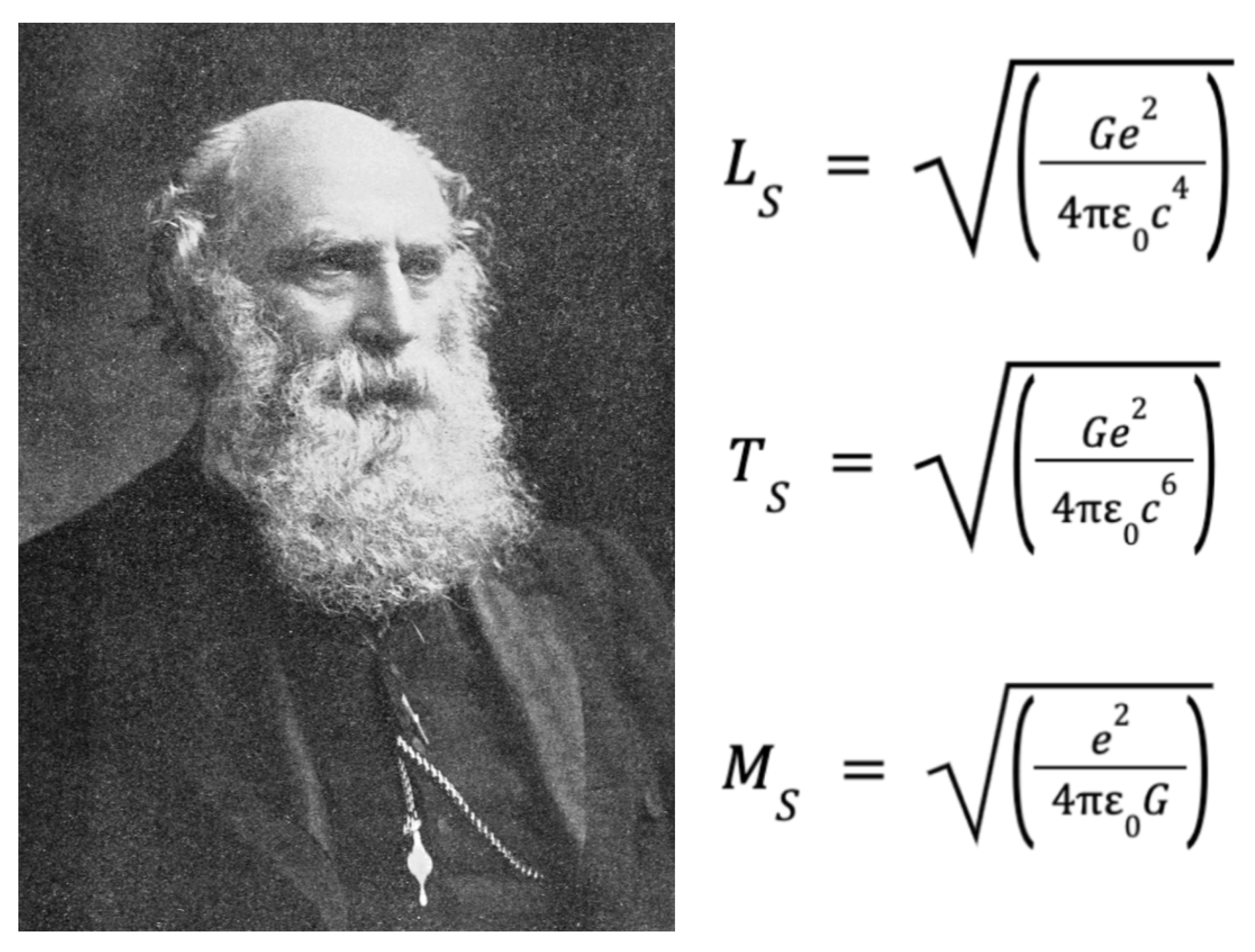
In this first system of natural units, the fundamental natural Stoney unit of angular momentum is given by,
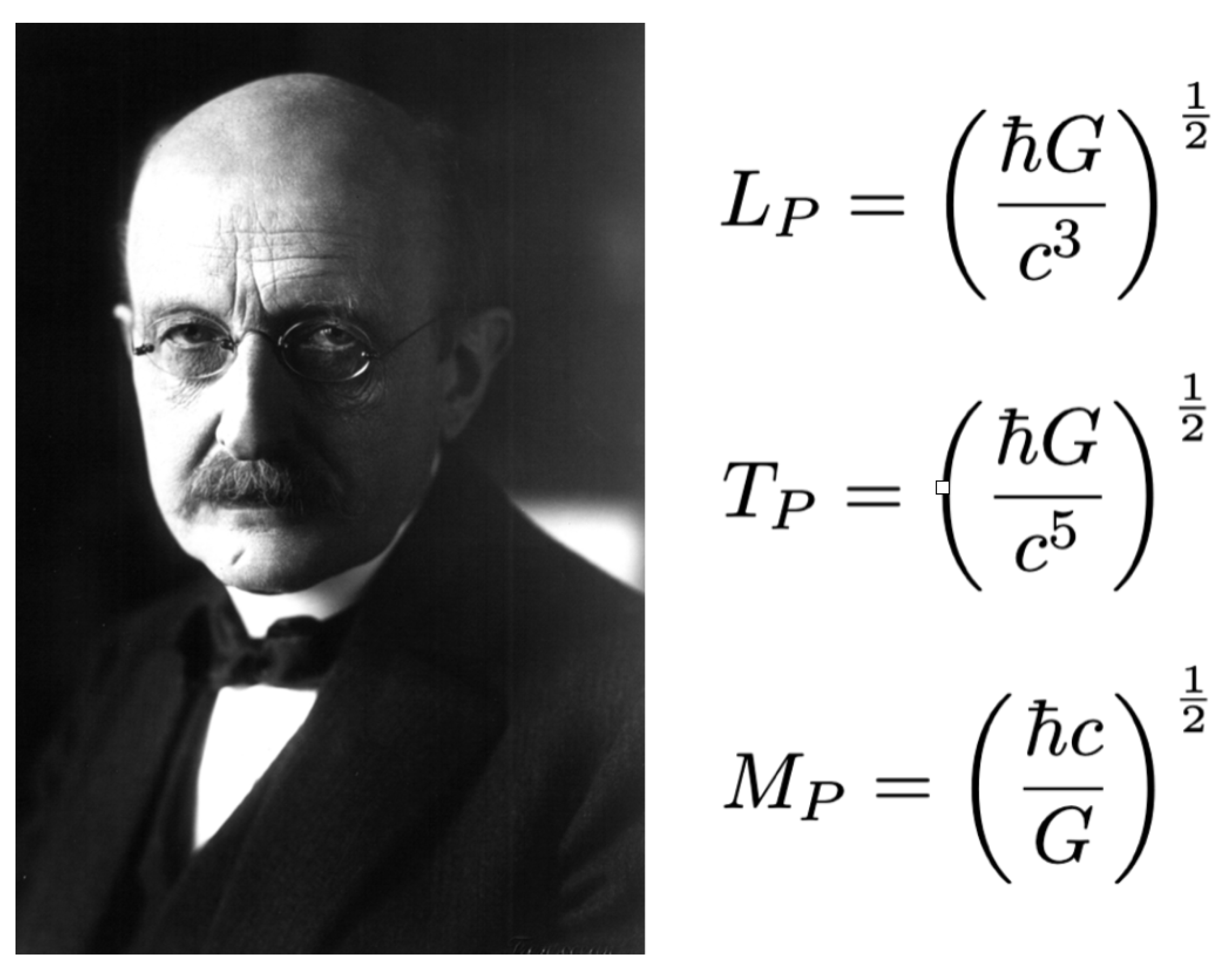
Once Planck uncovered ℏ, his quantum of action [41], denoting a universal lower bound on angular momentum where,
the Stoney system became subsumed into the Planck scale. See Figure B2.
Figure B2.
Max Planck’s discovery of his quantum of action, ℏ subsumed the existing Stoney system of natural units, into the Planck scale. Yet, the scale is the theoretical source of the catastrophic energy density of the vacuum (See Section 8); a universal expansion rate in which the universe should double in size every [4,33,38,52]. The observation of an accelerated expansion[1,2] and the realisation that , suggests such Planckian pathologies result from an incomplete quantum scale, without , setting a fundamental entropic bound and limit in nature (See Section 2.2). Just as the emergence of the FSC, reflected the emergence of Planck’s new scale from the Stoney system, the dimensionless GFSC, becomes its gravitational analogue, pointing to a more fundamental quantum scale in nature, the -scale. Image created by the author using public-domain source material.
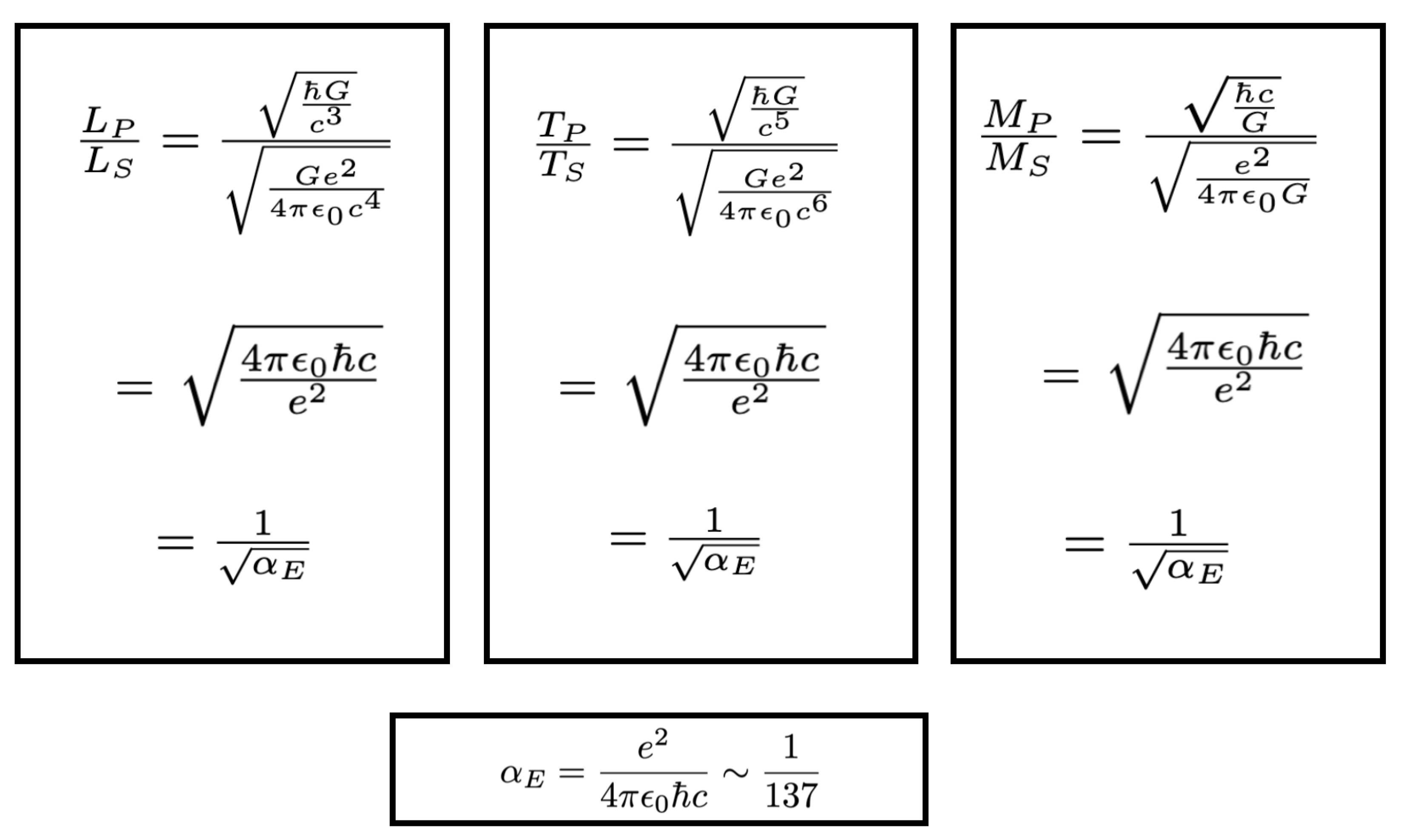
The ratio between the two angular momenta, both in units of is simply the FSC given by,
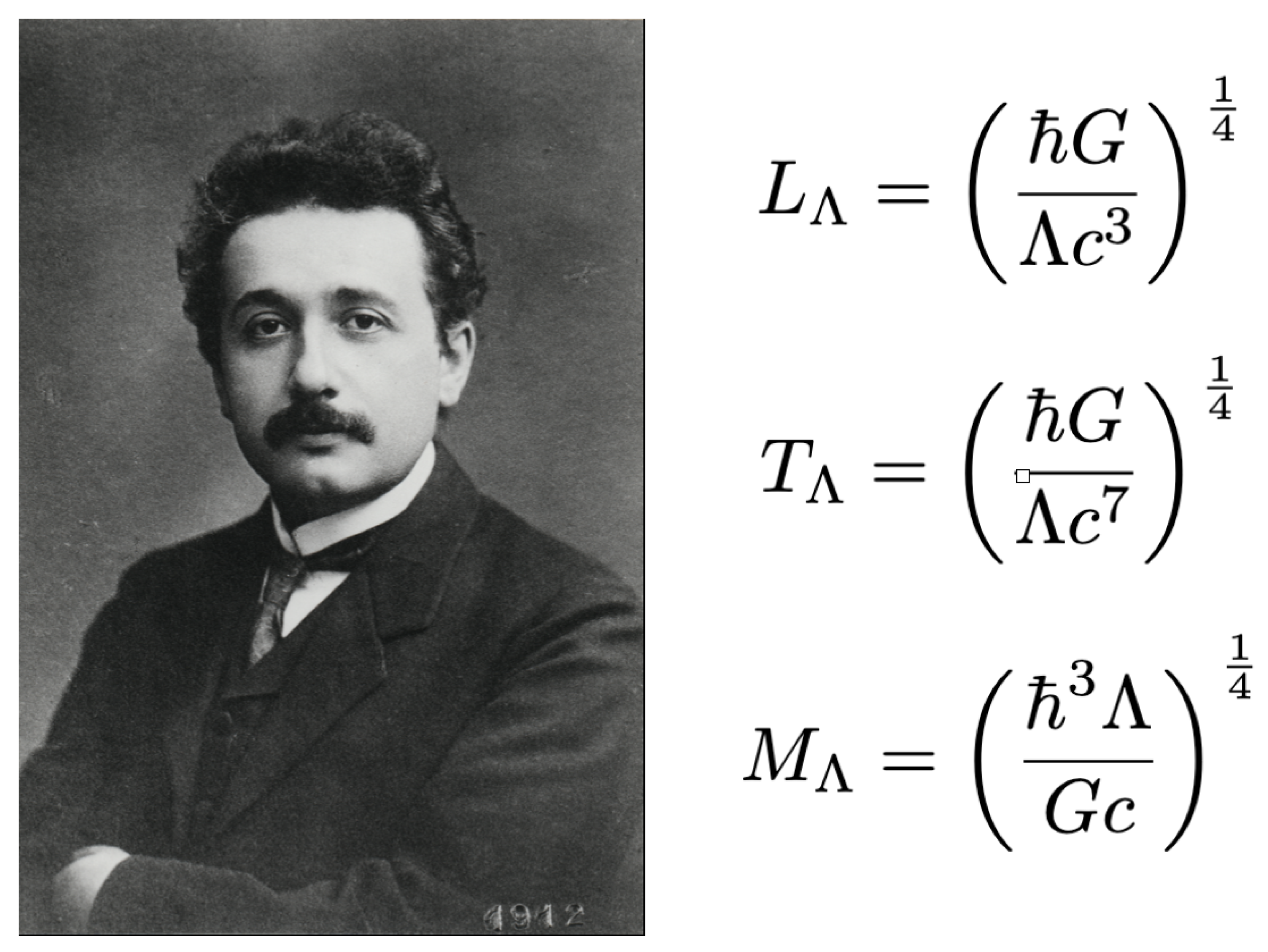
Although the world of physics was introduced to the FSC in 1916 when Sommerfeld observed the fine splitting of hydrogen spectral lines [74], it could have in theory been introduced much earlier by Planck himself once his quantum of action was discovered. The FSC is therefore a ratio of two like dimensioned quantities - angular momentum in Stoney units and that of ℏ itself, not some ’magical’ relationship between several, seemingly unrelated constants [75,76]. We find the -scale, see Figure B3, becomes its natural successor.
Figure B3.
The Lambda scale cannot emerge from dimensional analysis alone. An infinite number of possibilities represented by the affine family (A13) is the consequence. Whilst the Planck system maps three constants on to three base dimensions [M],[L],[T], uniqueness comes for free. However, the requirement of mapping four constants and on to the same three base dimensions, leaves an extra degree of freedom () in (A13). Physics fixes by the vacuum–matching postulate: the requirement that the resulting ZPE density, matches the vacuum energy from GR (See Eq. A14). The inclusion of Einstein’s cosmological constant becomes a thermodynamic completion of his gravitational vision, represented in Box 10.1. Rather than a historical blunder, it is simultaneously a necessity and a constraint, an inevitable consequence of its thermodynamic foundation. Image created by the author using public-domain source material.
In GR, has the dimensions of an inverse length squared or simply an inverse unit area in , thus,
In the Planck system, a unit inverse area is the inverse of the Planck length squared:
Thus the ratio of the two is also a comparison of like dimensions, both inverse unit areas, yields the GFSC ,
In gravitational physics, the cosmological constant is simply interpreted as a vacuum energy density. However, thermodynamics suggests the energy of a system is tied to its entropy (E = TS), thus is also a measure of entropy, that transforms the Bekenstein-Hawking bound into a fundamental upper limit of entropy for the -universe.
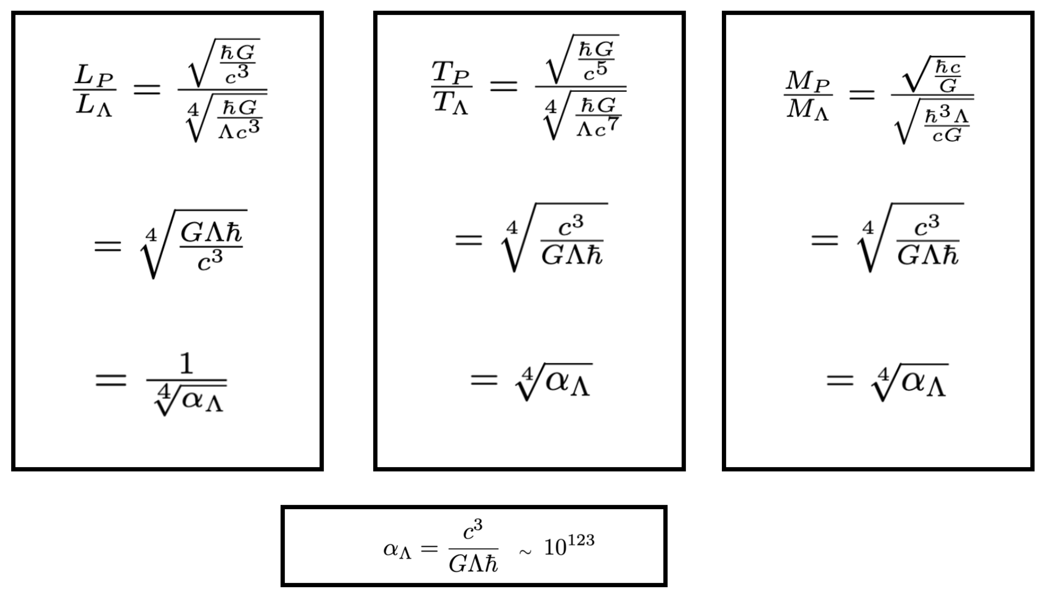
Where is just the cosmological constant in its dimensionless form. The consequences of Lambda’s introduction into physics finds a historical parallel with the shift from Stoney to Planck units, once ℏ was discovered [16]. If is considered a fundamental constant of nature and is incorporated into physics, then a new ‘natural scale’ emerges - the -scale. Like its Planck predecessor whose base and derived quantaties differ by factors of respectively from their Stoney counterparts, see Figure B4, the Lambda base and derived units differ from their Planck counterparts by , see Figure B5.
Just as encodes a limit on action, encodes a universal bound on gravitational entropy. The Lambda scale is thus not an arbitrary extension, but the natural successor to the Planck system — and the only one consistent with a finite vacuum entropy.
Figure B4.
The Planck scale differs from their Stoney counterparts by factors of the square root of the FSC, .
Figure B4.
The Planck scale differs from their Stoney counterparts by factors of the square root of the FSC, .
With c, ℏ, and now , we arrive at a complete triad of fundamental constants — each defining a domain of limiting behavior: causality, action, and information capacity. A coherent system of natural units must reflect all three. The Lambda system grounded in thermodynamics and quantum field theory, achieves precisely this. See Figure B5. It not only resolves the vacuum catastrophe, but redefines the conditions under which all physical laws — including gravity — must operate (LoEC).
Figure B5.
The Planck scale differs from the -scale in an analogous manner to the Planck to Stoney ratios, but this time by factors involving the quartic root of the GFSC, .
Figure B5.
The Planck scale differs from the -scale in an analogous manner to the Planck to Stoney ratios, but this time by factors involving the quartic root of the GFSC, .
Historically, Stoney’s units were subsumed once ℏ was recognized as fundamental: adopting the Planck charge rewrites electromagnetism in terms of the dimensionless coupling . Analogously, adding furnishes an IR ingredient: vacuum matching selects the length and packages gravity with the dimensionless . The –framework thus extends Planck’s by incorporating horizon thermodynamics.
In summary, once is recognised as a fundamental constant fixing a finite upper bound on the universe’s entropy [10,11], the Lambda scale emerges naturally as the successor to the Planck system. Dimensional analysis identifies as the geometric mean of the Planck length and the de Sitter radius [7,17]. This property, combined with the thermodynamic requirement that be constant, makes an inevitable new quantum length. Unlike the Planck scale, which overestimates the vacuum energy, the Lambda scale matches the observed value, aligning GR with thermodynamics and QFT, resolving the vacuum catastrophe [4].
Appendix C. Vacuum energy from Planck’s spectrum at T = 0 (consistency check)
Planck’s spectral energy density including the zero–point term [60,77,78] is
At the thermal part vanishes and the zero–point contribution remains:
Integrating up to a sharp UV cutoff gives
Equivalent k–space/mode–counting form. Quantizing the electromagnetic field, each mode contributes and the density of states per unit volume is . Then
since and .
- Matching to GR at the Λ scale.
The GR vacuum energy density is
Using the –scale cutoff (fixed by horizon thermodynamics / vacuum matching; see Section 8 and Eq. A32)
Substituting (C6) into (C3) yields
Hence the zero–point integral at the cutoff reproduces the GR vacuum density exactly. Thus both the thermodynamic (Section 2.2) and canonical routes (Section 8) agree.
References
- Perlmutter, S.; et al. Measurements of Ω and Λ from 42 High-Redshift Supernovae. Astrophysical Journal 1999, 517, 565–586. https://doi.org/10.1086/307221. [CrossRef]
- Riess, A.G.; et al. Observational Evidence from Supernovae for an Accelerating Universe and a Cosmological Constant. Astronomical Journal 1998, 116, 1009–1038. https://doi.org/10.1086/300499. [CrossRef]
- Schmidt, B.P.; Suntzeff, N.B.; Phillips, M.M.; et al.. The High-Z Supernova Search: Measuring Cosmic Deceleration and Global Curvature of the Universe Using Type Ia Supernovae. The Astrophysical Journal 1998, 507, 46–63. https://doi.org/10.1086/306308. [CrossRef]
- Weinberg, S. The Cosmological Constant Problem. Reviews of Modern Physics 1989, 61, 1–23. https://doi.org/10.1103/RevModPhys.61.1. [CrossRef]
- Jacobson, T. Thermodynamics of Spacetime: The Einstein Equation of State. Physical Review Letters 1995, 75, 1260–1263. https://doi.org/10.1103/PhysRevLett.75.1260. [CrossRef]
- Verlinde, E.P. On the Origin of Gravity and the Laws of Newton. Journal of High Energy Physics 2011, 2011, 29. https://doi.org/10.1007/JHEP04(2011)029. [CrossRef]
- Padmanabhan, T. Thermodynamical Aspects of Gravity: New Insights. Reports on Progress in Physics 2010, 73, 046901, [arXiv:gr-qc/0911.5004]. https://doi.org/10.1088/0034-4885/73/4/046901. [CrossRef]
- Duff, M.J.; Okun, L.B.; Veneziano, G. Trialogue on the number of fundamental constants. Journal of High Energy Physics 2002, 2002, 023. https://doi.org/10.1088/1126-6708/2002/03/023. [CrossRef]
- Tiesinga, E.; Mohr, P.J.; Newell, D.B.; Taylor, B.N. The 2018 CODATA recommended values of the fundamental physical constants. Reviews of Modern Physics 2021, 93, 025010. https://doi.org/10.1103/RevModPhys.93.025010. [CrossRef]
- Gibbons, G.W.; Hawking, S.W. Cosmological event horizons, thermodynamics, and particle creation. Physical Review D 1977, 15, 2738–2751. https://doi.org/10.1103/PhysRevD.15.2738. [CrossRef]
- Bekenstein, J.D. Black holes and entropy. Physical Review D 1973, 7, 2333–2346. https://doi.org/10.1103/PhysRevD.7.2333. [CrossRef]
- Hawking, S.W. Particle creation by black holes. Communications in Mathematical Physics 1975, 43, 199–220. https://doi.org/10.1007/BF02345020. [CrossRef]
- Clausius, R. On Different Forms of the Fundamental Equations of the Mechanical Theory of Heat and their Convenience for Application. Annalen der Physik 1865, 125, 353–400.
- Bousso, R. Positive Vacuum Energy and the N-Bound. Journal of High Energy Physics 2000, 2000, 038, [arXiv:hep-th/hep-th/0010252]. https://doi.org/10.1088/1126-6708/2000/11/038. [CrossRef]
- Dyson, L.; Kleban, M.; Susskind, L. Disturbing Implications of a Cosmological Constant. Journal of High Energy Physics 2002, 2002, 011, [hep-th/0208013]. https://doi.org/10.1088/1126-6708/2002/10/011. [CrossRef]
- Planck, M. Über irreversible Strahlungsvorgänge. Sitzungsberichte der Königlich Preußischen Akademie der Wissenschaften zu Berlin 1899, pp. 440–480.
- Zeldovich, Y.B. Cosmological Constant and Elementary Particles. JETP Letters 1967, 6, 316. Reprinted in Sov. Phys. Usp. 11 (1968) 381.
- Bardeen, J.M.; Carter, B.; Hawking, S.W. The Four Laws of Black Hole Mechanics. Communications in Mathematical Physics 1973, 31, 161–170. https://doi.org/10.1007/BF01645742. [CrossRef]
- Hawking, S.W. Black hole explosions? Nature 1974, 248, 30–31. https://doi.org/10.1038/248030a0. [CrossRef]
- Unruh, W.G. Notes on black-hole evaporation. Physical Review D 1976, 14, 870–892. https://doi.org/10.1103/PhysRevD.14.870. [CrossRef]
- ’t Hooft, G. Dimensional reduction in quantum gravity. arXiv preprint gr-qc/9310026 1993.
- Susskind, L. The world as a hologram. Journal of Mathematical Physics 1995, 36, 6377–6396. https://doi.org/10.1063/1.531249. [CrossRef]
- Bousso, R. A covariant entropy conjecture. Journal of High Energy Physics 1999, 07, 004. https://doi.org/10.1088/1126-6708/1999/07/004. [CrossRef]
- Clausius, R. On the Motive Power of Heat, and on the Laws which can be deduced from it for the Theory of Heat. Annalen der Physik 1850, 79, 368–397. English translation in Phil. Mag. 2 (1851) 1.
- Griffiths, D.J. Introduction to Electrodynamics, 4th ed.; Cambridge University Press, 2017.
- Poynting, J.H. On the Transfer of Energy in the Electromagnetic Field. Philosophical Transactions of the Royal Society of London 1884, 175, 343–361.
- Jackson, J.D. Classical Electrodynamics, 3rd ed.; Wiley: New York, 1998.
- de Coulomb, C.A. Premier mémoire sur l’électricité et le magnétisme. Histoire de l’Académie Royale des Sciences 1785, pp. 569–577.
- Sommerfeld, A. Zur Quantentheorie der Spektrallinien. Annalen der Physik 1916, 356, 1–94.
- Casimir, H.B.G. On the Attraction Between Two Perfectly Conducting Plates. Proc. K. Ned. Akad. Wet. 1948, 51, 793–795.
- Lamoreaux, S.K. Demonstration of the Casimir Force in the 0.6 to 6 μm Range. Physical Review Letters 1997, 78, 5–8. https://doi.org/10.1103/PhysRevLett.78.5. [CrossRef]
- Jaffe, R.L. The Casimir Effect and the Quantum Vacuum. Physical Review D 2005, 72, 021301. https://doi.org/10.1103/PhysRevD.72.021301. [CrossRef]
- Padmanabhan, T. Cosmological constant: The weight of the vacuum. Physics Reports 2003, 380, 235–320. https://doi.org/10.1016/S0370-1573(03)00120-0. [CrossRef]
- Mostepanenko, V.M.; Trunov, N.N. The Casimir Effect and its Applications. Physics-Uspekhi 2001, 44, 493–509. https://doi.org/10.1070/PU2001v044n05ABEH000939. [CrossRef]
- Lifshitz, E.M. The Theory of Molecular Attractive Forces Between Solids. Soviet Physics JETP 1956, 2, 73–83.
- Pathria, R.K. Statistical Mechanics, 2nd ed.; Butterworth-Heinemann: Oxford, 1996.
- Kolb, E.W.; Turner, M.S. The Early Universe; Vol. 69, Frontiers in Physics, Addison-Wesley: Redwood City, CA, 1990.
- Martin, J. Everything You Always Wanted To Know About The Cosmological Constant Problem (But Were Afraid To Ask). C. R. Phys. 2012, 13, 566–665. https://doi.org/10.1016/j.crhy.2012.04.008. [CrossRef]
- Burgess, C.P. The Cosmological Constant Problem: Why it’s hard to get Dark Energy from Micro-physics. In Post-Planck Cosmology; Deffayet, C.; Peter, P., Eds.; Oxford University Press: Oxford, 2015; Vol. 100, Lecture Notes of the Les Houches Summer School, pp. 149–197, [arXiv:hep-th/1309.4133]. https://doi.org/10.1093/acprof:oso/9780198728856.003.0004. [CrossRef]
- Boltzmann, L. Über die Beziehung zwischen dem zweiten Hauptsatze der mechanischen Wärmetheorie und der Wahrscheinlichkeitsrechnung respektive den Sätzen über das Wärmegleichgewicht. Sitzungsberichte der Kaiserlichen Akademie der Wissenschaften, Mathematisch-Naturwissenschaftliche Classe 1877, 76, 373–435. English translation in: Ludwig Boltzmann, Theoretical Physics and Philosophical Problems, ed. B. McGuinness (Reidel, 1974).
- Planck, M. On the Law of Distribution of Energy in the Normal Spectrum. Annalen der Physik 1901, 4, 553–563. https://doi.org/10.1002/andp.19013090310. [CrossRef]
- Riess, A.G.; Yuan, W.; Macri, L.M.; et al.. A Comprehensive Measurement of the Local Value of the Hubble Constant with 1 km s-1 Mpc-1 Uncertainty from the Hubble Space Telescope and the SH0ES Team. The Astrophysical Journal Letters 2022, 934, L7, [arXiv:astro-ph.CO/2112.04510]. https://doi.org/10.3847/2041-8213/ac5c5b. [CrossRef]
- Verde, L.; Schöneberg, N.; Gil-Marín, H. A Tale of Many H0. Annual Review of Astronomy and Astrophysics 2024, 62, 287–331. https://doi.org/10.1146/annurev-astro-052622-033813. [CrossRef]
- Einstein, A. Die Feldgleichungen der Gravitation. Sitzungsberichte der Königlich Preußischen Akademie der Wissenschaften (Berlin) 1915, pp. 844–847.
- Einstein, A. Kosmologische Betrachtungen zur allgemeinen Relativitätstheorie. Sitzungsberichte der Königlich Preußischen Akademie der Wissenschaften (Berlin) 1917, pp. 142–152. English translation: Cosmological Considerations in the General Theory of Relativity.
- Einstein, A. Letter to Georges Lemaître (1947). Collected Papers of Albert Einstein, Vol. 8, 1947. English translation available in the Princeton University Press edition.
- Newton, I. Philosophiæ Naturalis Principia Mathematica; Royal Society, 1687. English translation by I. Bernard Cohen and Anne Whitman, University of California Press, 1999.
- Weinberg, S. The Cosmological Constant Problem. Reviews of Modern Physics 1989, 61, 1–23. https://doi.org/10.1103/RevModPhys.61.1. [CrossRef]
- Martin, J. Everything You Always Wanted To Know About The Cosmological Constant Problem (But Were Afraid To Ask). Comptes Rendus Physique 2012, 13, 566–665, [arXiv:astro-ph.CO/1205.3365]. https://doi.org/10.1016/j.crhy.2012.04.008. [CrossRef]
- ’t Hooft, G. Naturalness, Chiral Symmetry, and Spontaneous Chiral Symmetry Breaking. In Proceedings of the Recent Developments in Gauge Theories; ’t Hooft et al., G., Ed., New York, 1980; pp. 135–157. https://doi.org/10.1007/978-1-4684-7571-5_9. [CrossRef]
- Giudice, G.F. Naturally speaking: The naturalness criterion and physics at the LHC. In Perspectives on LHC Physics; World Scientific, 2008; [arXiv:0801.2562].
- Carroll, S.M. The Cosmological Constant. Living Reviews in Relativity 2001, 4, 1. https://doi.org/10.12942/lrr-2001-1. [CrossRef]
- Peebles, P.J.E.; Ratra, B. The Cosmological Constant and Dark Energy. Reviews of Modern Physics 2003, 75, 559–606. https://doi.org/10.1103/RevModPhys.75.559. [CrossRef]
- Copeland, E.J.; Sami, M.; Tsujikawa, S. Dynamics of dark energy. International Journal of Modern Physics D 2006, 15, 1753–1936, [hep-th/0603057]. https://doi.org/10.1142/S021827180600942X. [CrossRef]
- Sola, J. Cosmological constant and vacuum energy: old and new ideas. In Proceedings of the Journal of Physics: Conference Series. IOP Publishing, 2013, Vol. 453, p. 012015.
- Solà, J.; Gómez-Valent, A.; de Cruz Pérez, J. Hints of dynamical vacuum energy in the expanding Universe. The Astrophysical Journal 2015, 811, L14, [arXiv:astro-ph.CO/1506.05793]. https://doi.org/10.1088/2041-8205/811/2/L14. [CrossRef]
- Hu, J.P.; Wang, F.Y. Hubble Tension: The Evidence of New Physics. Universe 2023, 9, 94, [2302.05709]. https://doi.org/10.3390/universe9020094. [CrossRef]
- Sakharov, A.D. Vacuum Quantum Fluctuations in Curved Space and the Theory of Gravitation. Soviet Physics Doklady 1968, 12, 1040–1041. Reprinted in Gen. Relativ. Gravit. 32, 365 (2000).
- Plunien, G.; Müller, B.; Greiner, W. The Casimir effect. Physics Reports 1986, 134, 87–193. https://doi.org/10.1016/0370-1573(86)90020-7. [CrossRef]
- Milonni, P.W. The Quantum Vacuum: An Introduction to Quantum Electrodynamics; Academic Press: San Diego, CA, 1994.
- Burgess, C.P. The Cosmological Constant Problem: Why it’s hard to get Dark Energy from Micro-physics. arXiv preprint arXiv:1309.4133 2013, [arXiv:hep-th/1309.4133].
- Padilla, A. Lectures on the Cosmological Constant Problem. arXiv preprint 2015, [arXiv:hep-th/1502.05296].
- Barrow, J.D. The Constants of Nature. Nature 1995, 376, 321–322. https://doi.org/10.1038/376321a0. [CrossRef]
- Wilczek, F. Scaling Mount Planck II: Base Camp. Physics Today 2005, 58, 12–13. https://doi.org/10.1063/1.2138456. [CrossRef]
- Eddington, A.S. The Mathematical Theory of Relativity; Cambridge University Press: Cambridge, 1923.
- Strominger, A. The dS/CFT Correspondence. Journal of High Energy Physics 2001, 10, 034, [hep-th/0106113]. https://doi.org/10.1088/1126-6708/2001/10/034. [CrossRef]
- Banks, T. Some Thoughts on the Quantum Theory of Stable de Sitter Space. Journal of High Energy Physics 2005, 03, 048, [hep-th/0503066]. https://doi.org/10.1088/1126-6708/2005/03/048. [CrossRef]
- Planck, M. On the Theory of the Law of Energy Distribution in the Normal Spectrum. Verhandlungen der Deutschen Physikalischen Gesellschaft 1900, 2, 237–245.
- Kuhn, T.S. Black-Body Theory and the Quantum Discontinuity, 1894–1912; Oxford University Press, 1978.
- Buckingham, E. On Physically Similar Systems; Illustrations of the Use of Dimensional Equations. Phys. Rev. 1914, 4, 345–376. https://doi.org/10.1103/PhysRev.4.345. [CrossRef]
- Stoney, G.J. On the Physical Units of Nature. Philosophical Magazine 1881, 11, 381–390. https://doi.org/10.1080/14786448108627031. [CrossRef]
- Heaviside, O. Electromagnetic Theory; Vol. 1, The Electrician Printing and Publishing Co., 1893. Historical origin of rationalized electromagnetic units.
- Particle Data Group. Review of Particle Physics. Progress of Theoretical and Experimental Physics 2024, 2024, 083C01. Conventions section summarizes natural units and Heaviside–Lorentz EM usage, https://doi.org/10.1093/ptep/ptae080. [CrossRef]
- Sommerfeld, A. Zur quantentheorie der spektrallinien. Annalen der Physik 1916, 356, 1–94.
- Feynman, R.P.; Leighton, R.B.; Sands, M.L. The Feynman Lectures on Physics: electromagnetism and matter; Vol. 2, Addison-Wesley Publishing Company, 1964.
- Dirac, P.A.M. The Cosmological Constants. Nature 1937, 139, 323. https://doi.org/10.1038/139323a0. [CrossRef]
- Planck, M. Über eine Verbesserung der Wien’schen Spektralgleichung. Verhandlungen der Deutschen Physikalischen Gesellschaft 1911, 13, 138–175.
- Nernst, W. Über einen Versuch, aus der Quantenhypothese und der Gasgleichung die Strahlungsgleichung herzuleiten. Verhandlungen der Deutschen Physikalischen Gesellschaft 1916, 18, 83–116.
Figure 1.
The Lambda scale emerges once the cosmological constant is recognized as a fundamental constant of nature, fixing the total entropy of the universe. The Planck system, whilst being a self-consistent set of natural units, is thermodynamically sterile: it omits the vacuum contribution. Once included the -scale supersedes the Planck scale as the physically complete framework, embedding vacuum thermodynamics in its foundations. [Notation. We denote the –base units by (length), (time), (mass), and (temperature). In formulas, T denotes a physical temperature; the temperature unit is . Dimensions remain , , ]. See Appendix A.
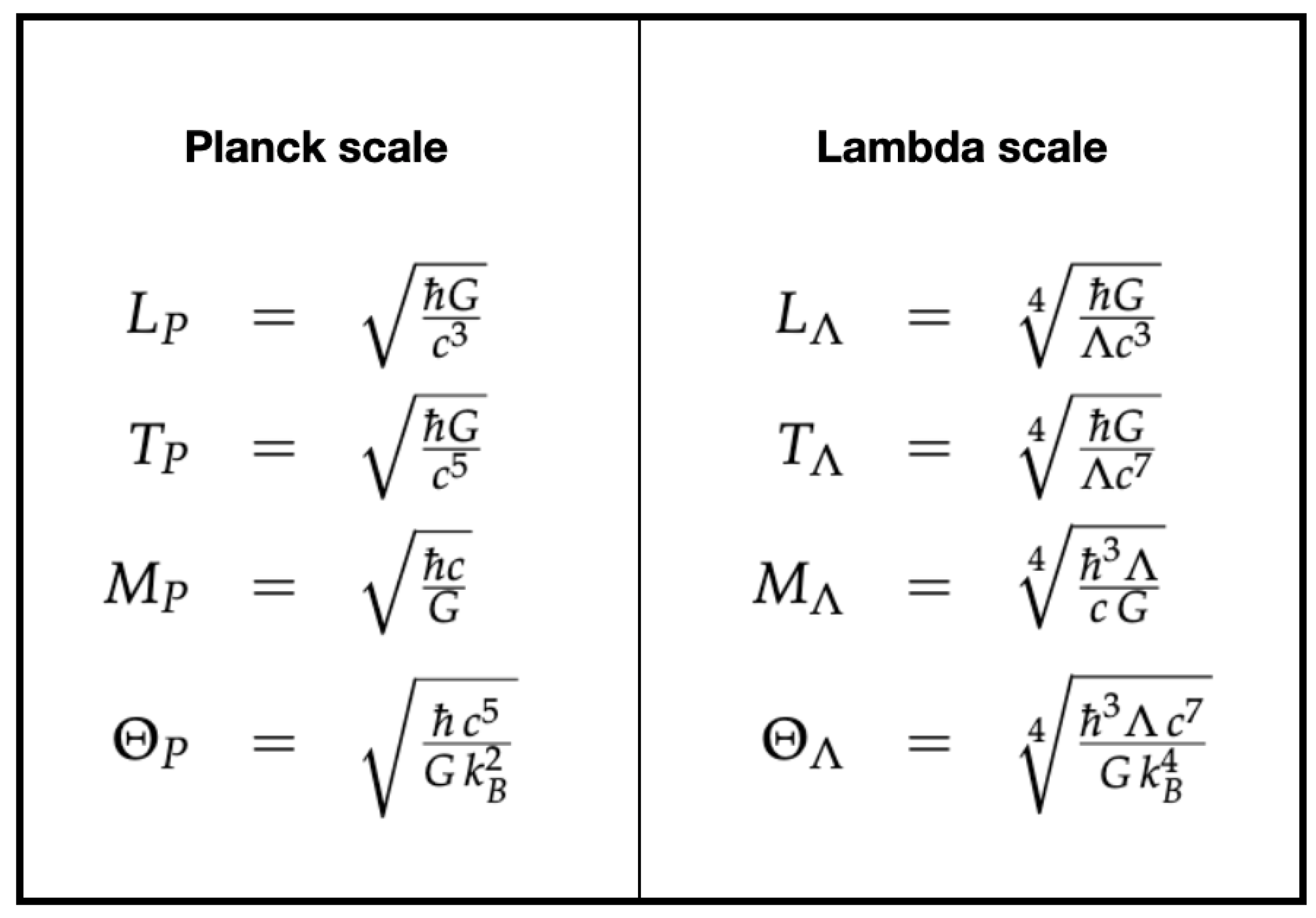
Figure 2.
The four laws of black hole thermodynamics, shown here for Rindler, Schwarzschild, and de Sitter horizons. Originally formulated for stationary black holes, these laws reveal a profound connection between gravity, entropy, and temperature. They are now understood to reflect the causal structure of spacetime itself, applying to any causal boundary [10,12,19,20]
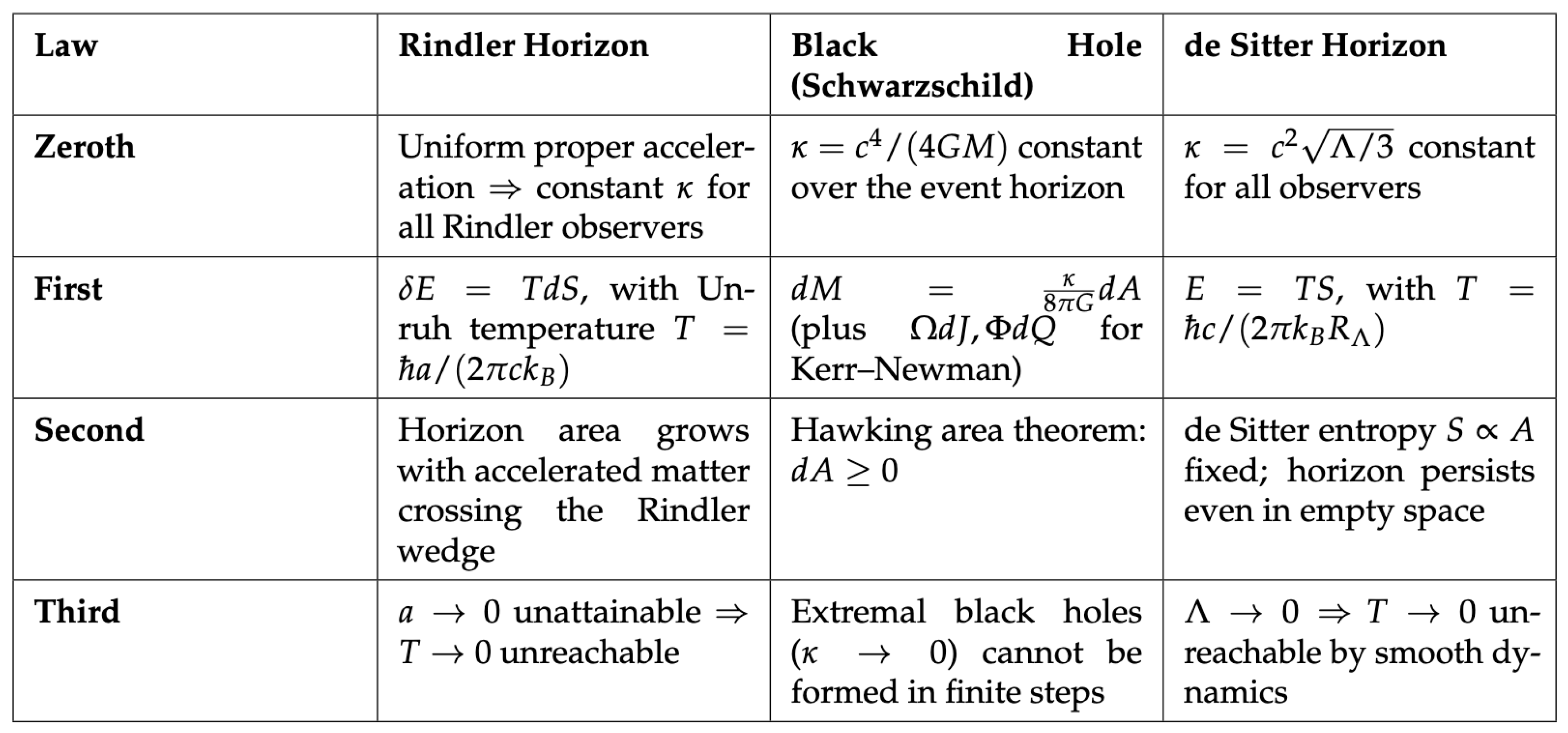
Figure 3.
Rindler wedge for a uniformly accelerated observer with proper acceleration a. A causal horizon forms at proper distance . For this observer the Minkowski vacuum is a thermal equilibrium state with Unruh temperature , so a comoving detector responds as if immersed in a thermal bath—while inertial observers register no flux (observer dependence). For the Rindler horizon we quote entropy per unit transverse area, .
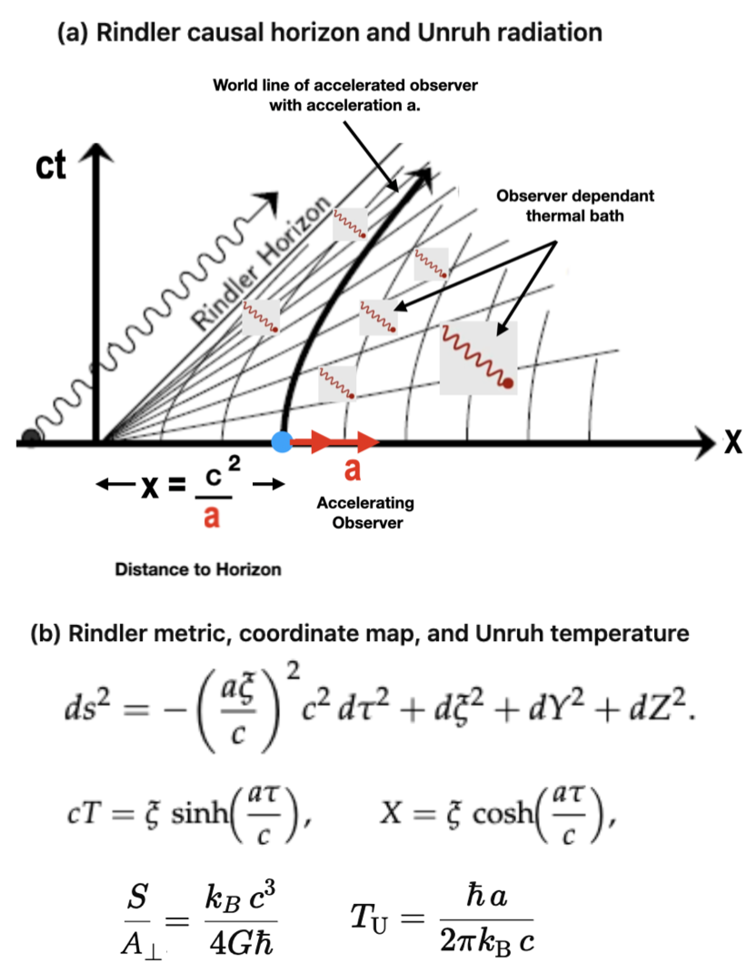
Figure 4.
Hawking radiation. Quantum fluctuations at a black hole horizon produce entangled pairs; one particle escapes as radiation while its partner falls in. The effect illustrates the universal thermality of horizons.
Figure 4.
Hawking radiation. Quantum fluctuations at a black hole horizon produce entangled pairs; one particle escapes as radiation while its partner falls in. The effect illustrates the universal thermality of horizons.
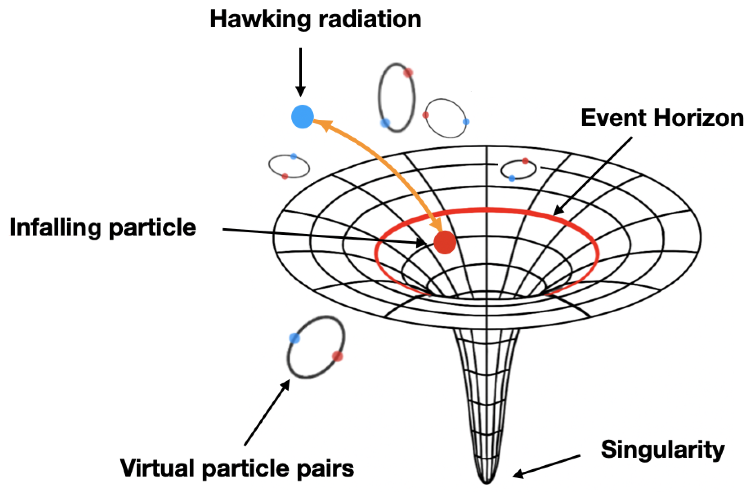
Figure 5.
Schwarzschild spacetime. Penrose–Carter diagram showing the causal structure of a black hole: singularity (wavy line), event horizon (dashed line), and infinities.
Figure 5.
Schwarzschild spacetime. Penrose–Carter diagram showing the causal structure of a black hole: singularity (wavy line), event horizon (dashed line), and infinities.
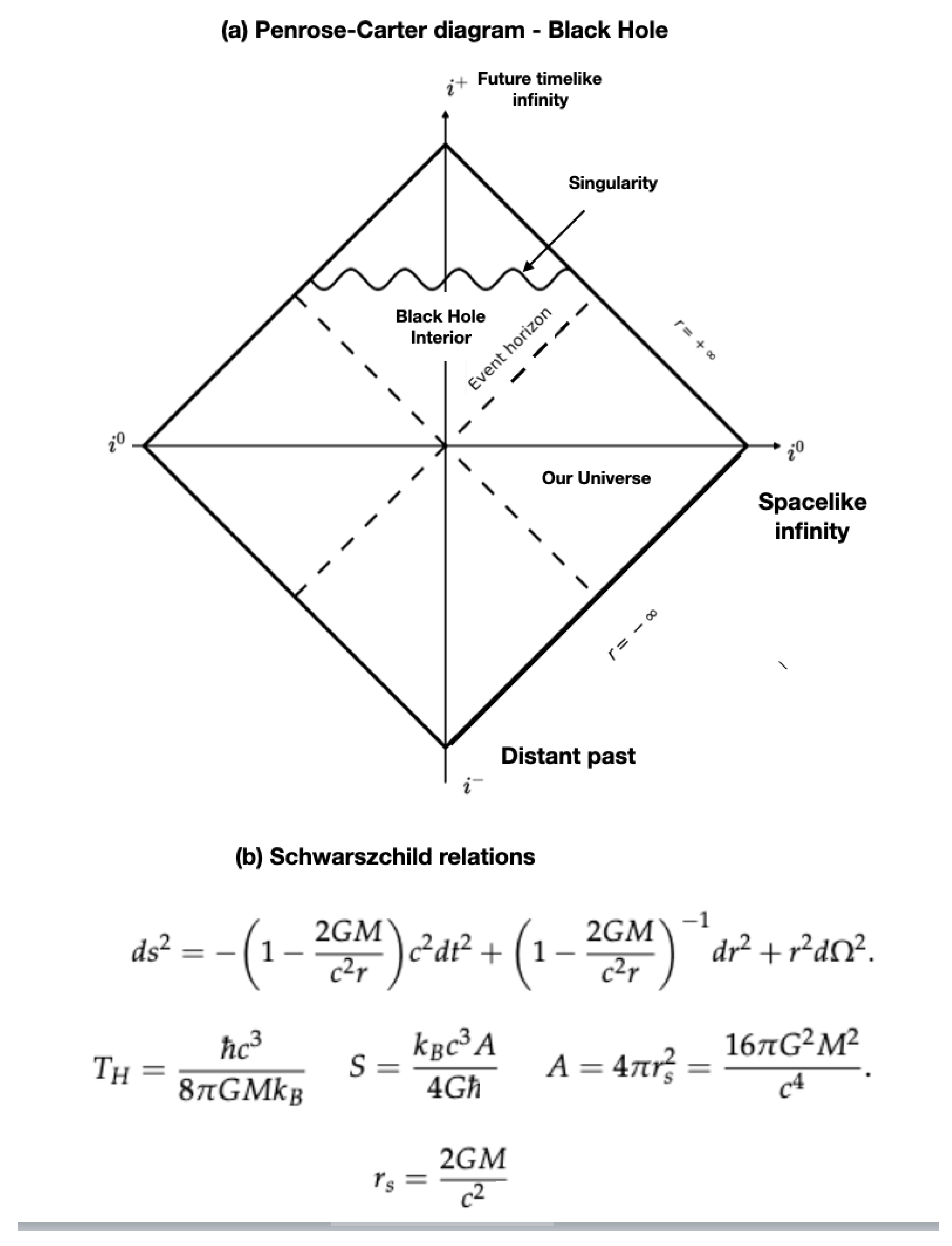
Figure 6.
de Sitter horizon. The causal diamond of a comoving observer defines the finite entropy accessible in an expanding universe, establishing a universal bound on information capacity. labels the (future) horizon; H is the Hubble rate. The de Sitter radius is .
Figure 6.
de Sitter horizon. The causal diamond of a comoving observer defines the finite entropy accessible in an expanding universe, establishing a universal bound on information capacity. labels the (future) horizon; H is the Hubble rate. The de Sitter radius is .
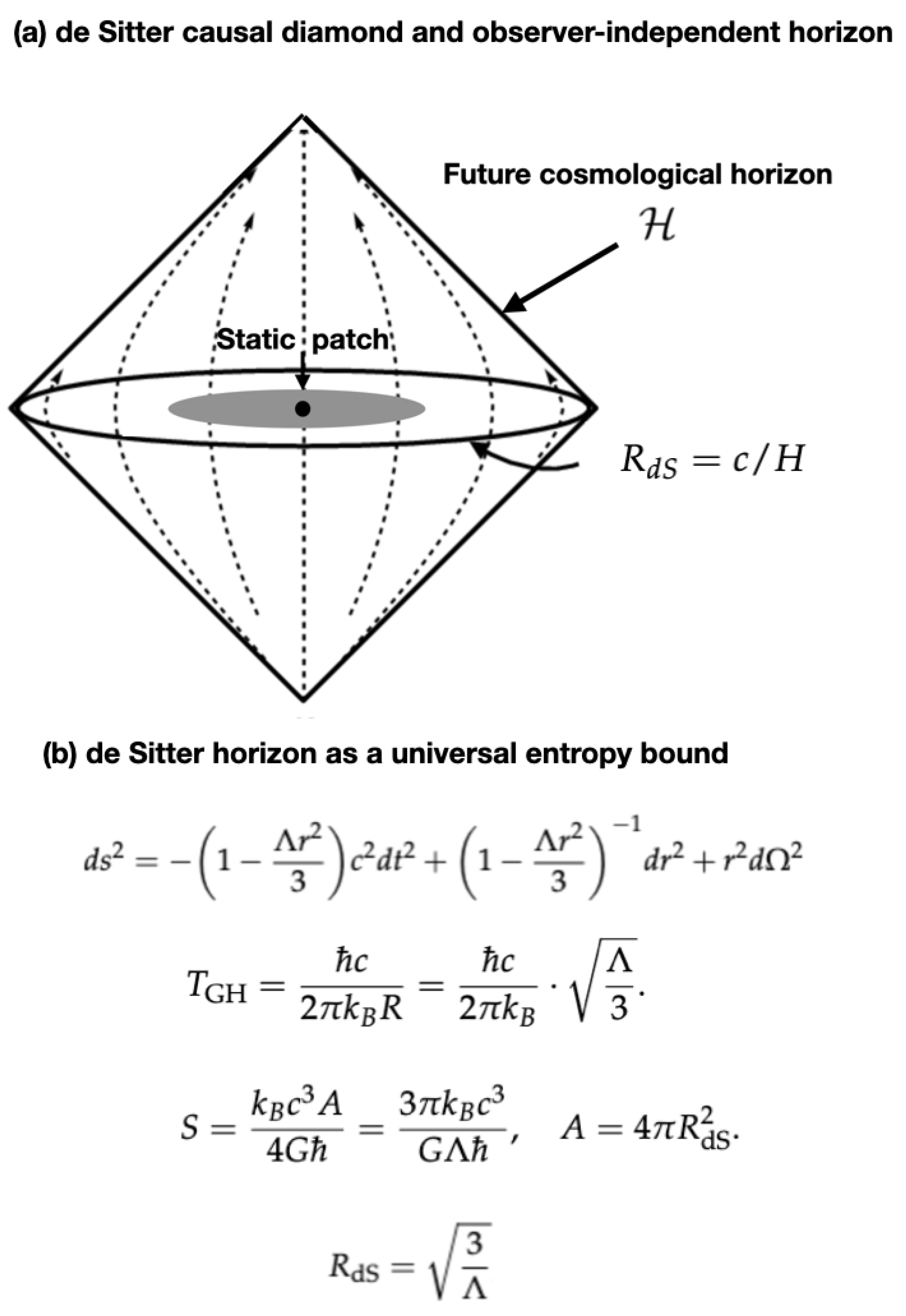
Figure 7.
An energy density in in base units will have the dimensions the result has exactly the dimensional form as the energy density of the vacuum that emerges in GR (without geometric normalisation), demonstrating the elegance and simplicity through which the vacuum catastrophe is abolished. The geometric factor arises only upon matching to the GR source term (horizon geometry / Einstein equations); see Section 8 and Appendix C. From the standpoint of the -scale the vacuum catastrophe is a physicist’s ghost.
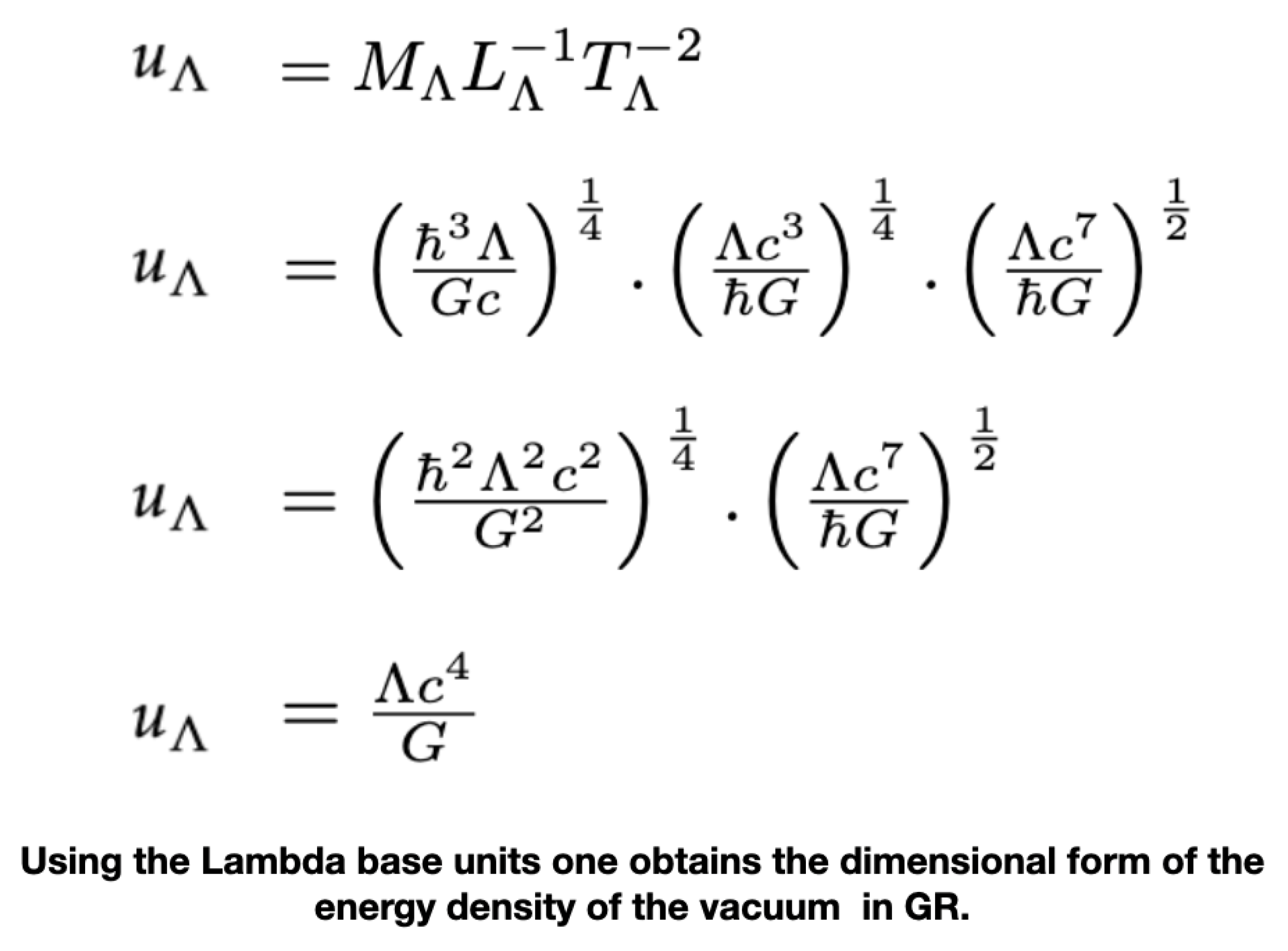
Figure 8.
Force scales in -units. The second row lists the base quantities required for each case: for inertia, for gravity, and for electromagnetism. Here is the electromagnetic fine-structure constant (FSC).
Figure 8.
Force scales in -units. The second row lists the base quantities required for each case: for inertia, for gravity, and for electromagnetism. Here is the electromagnetic fine-structure constant (FSC).
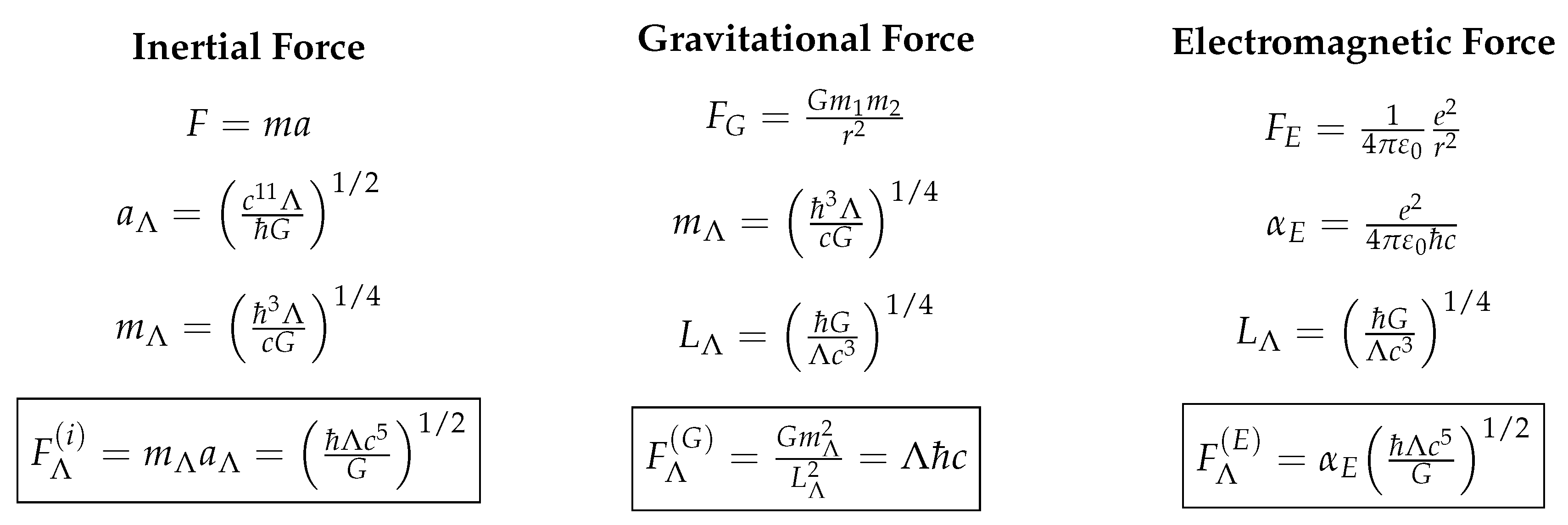
Figure 9.
The Casimir effect arises from the suppression of vacuum fluctuations between closely spaced plates, yielding a greater vacuum pressure outside the plates compared to that inside, resulting in a measurable attractive force. As a direct manifestation of zero-point energy, this phenomenon provides a laboratory probe into the structure of the vacuum — and when correctly interpreted, links directly to the cosmological constant .
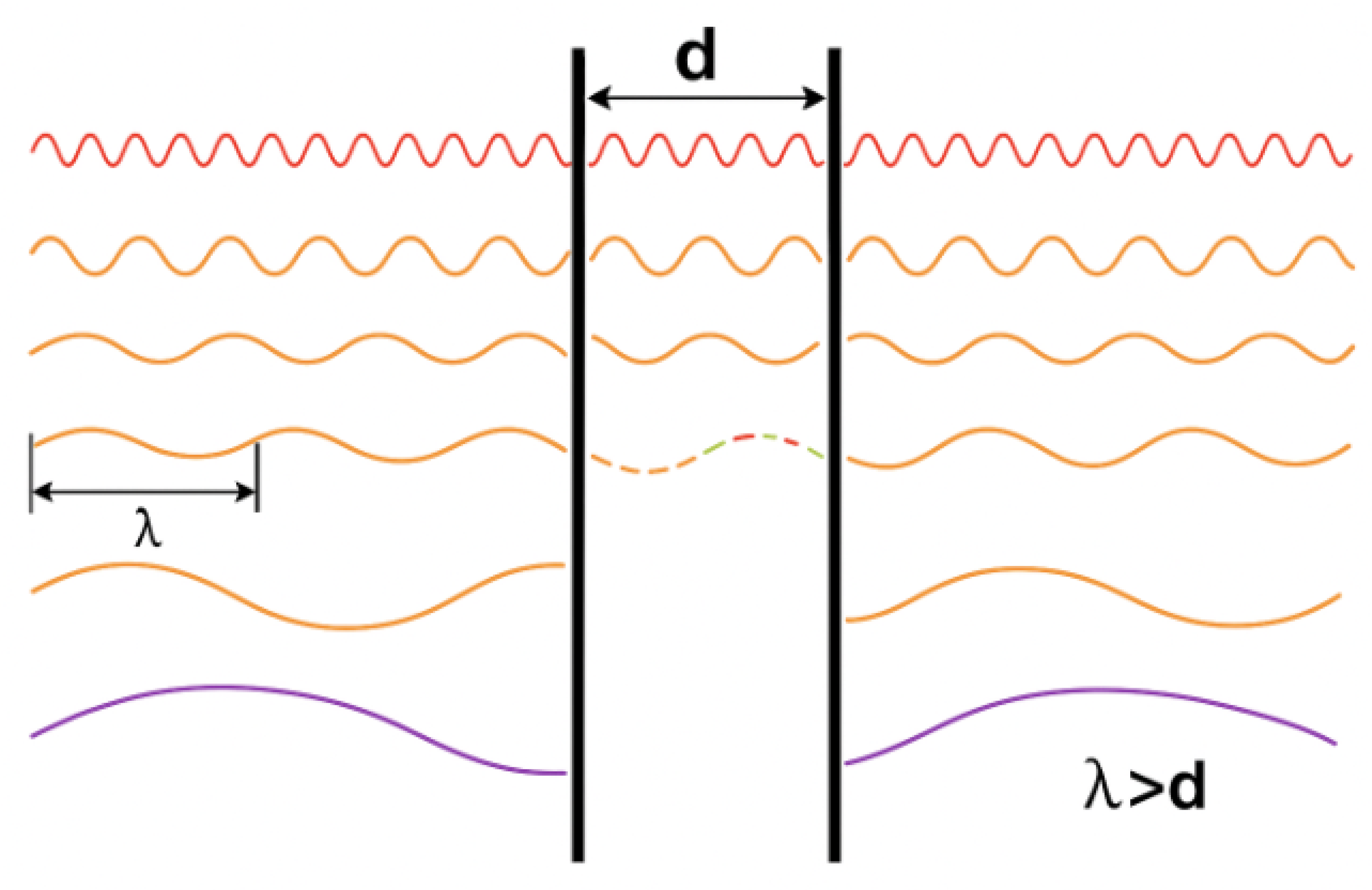
Figure 10.
Connecting the standard Casimir pressure with GR’s vacuum density. At the –length , Eq. 24 gives , i.e. the same negative pressure (tension) as the GR vacuum (). The -scale shows they are the same quantity up to a dimensionless factor of order unity, making the quantum vacuum and the cosmological vacuum one and the same in this framework.
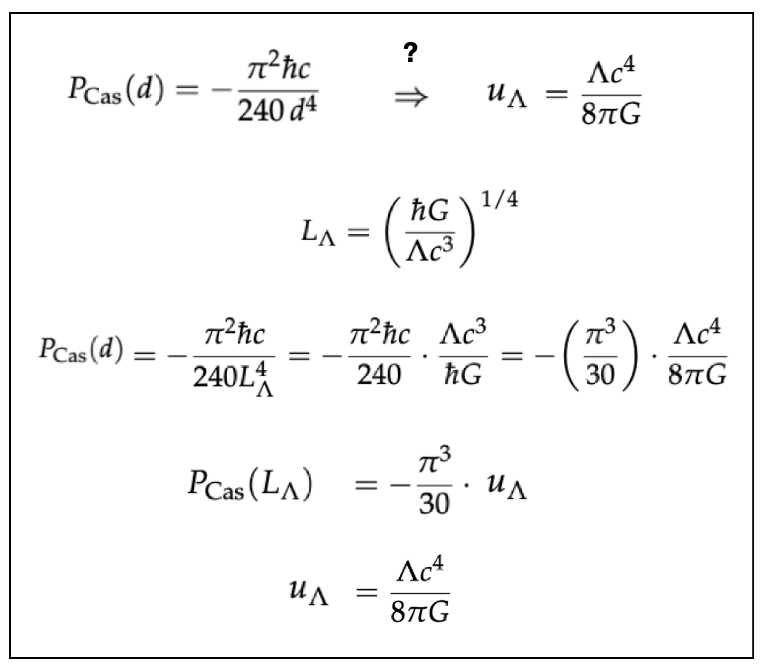
Figure 11.
Casimir pressure versus plate separation. The ideal law (black) meets the vacuum ceiling (red) at a crossover distance . Measuring determines the cosmological constant, . For ideal reflectors the crossover is with ; material/thermal corrections are handled in the Lifshitz framework.
Figure 11.
Casimir pressure versus plate separation. The ideal law (black) meets the vacuum ceiling (red) at a crossover distance . Measuring determines the cosmological constant, . For ideal reflectors the crossover is with ; material/thermal corrections are handled in the Lifshitz framework.
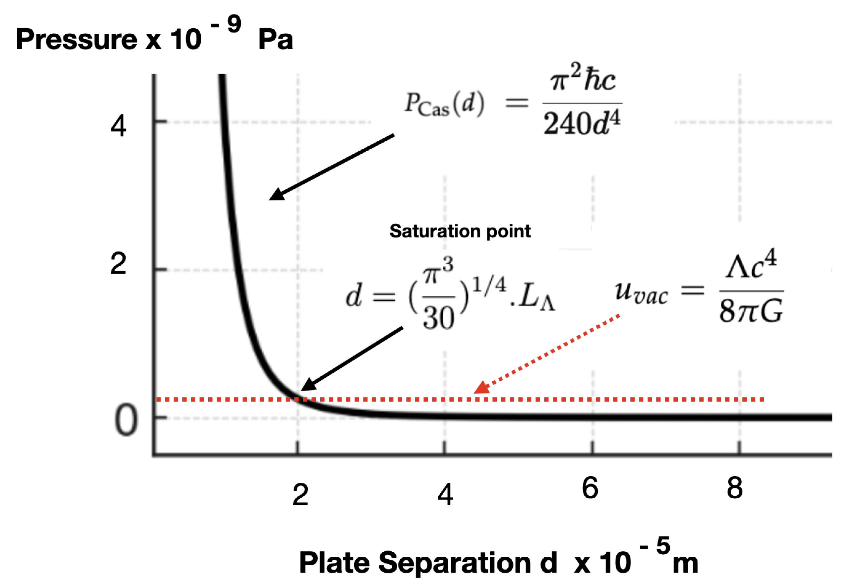
Figure 12.
Log–log view of vs. d. The black line shows the trend (slope ); the red line marks the vacuum ceiling. Their intersection defines , from which follows. Arrow indicates the micron–tens-of-microns crossover scale [31,35].
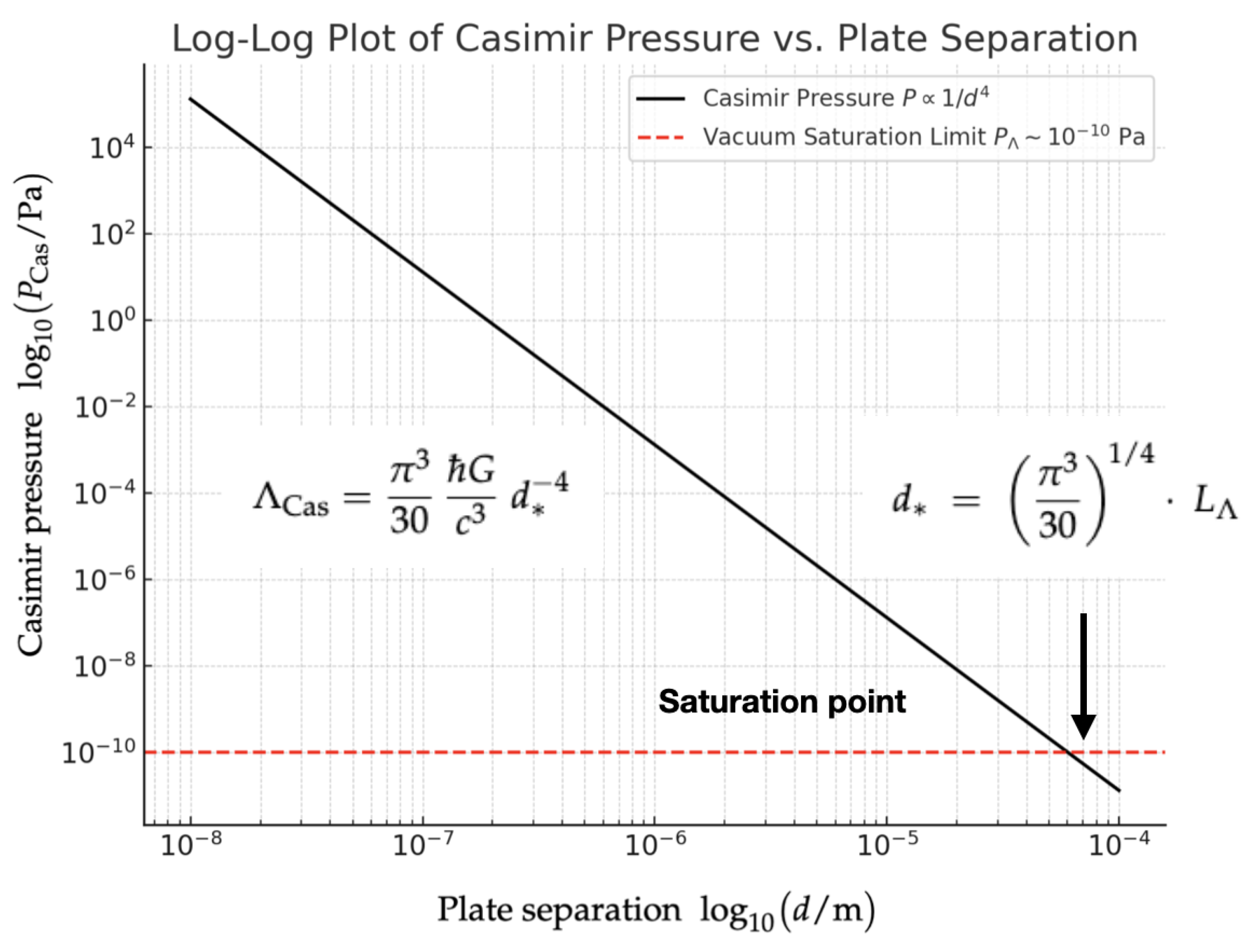
Figure 13.
Bosons (photons, ) and fermions (relic neutrinos, ) at the -temperature : , and at both become fixed fractions of ( shown).
Figure 13.
Bosons (photons, ) and fermions (relic neutrinos, ) at the -temperature : , and at both become fixed fractions of ( shown).
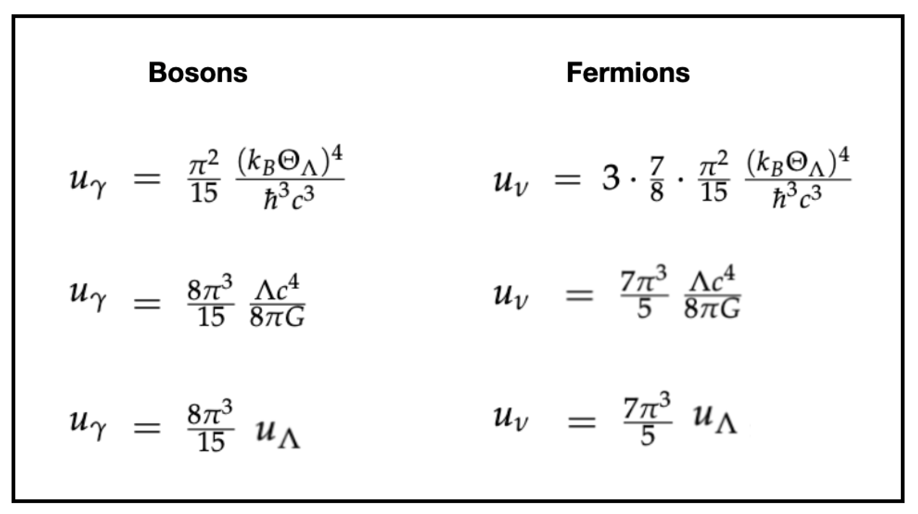
Figure 14.
Newton’s cosmological constant. (a) Newton showed that spherical symmetry permits two central force laws: an inverse–square attraction, , and a linear (harmonic) term . Both combine naturally into the general two–term form . (b) In general relativity, the second Friedmann equation in the weak–field dust limit yields the force law , which likewise reduces to the unified form . Note. The term is a Hooke-like tensional contribution (units: force/length, i.e. ). In GR with a cosmological constant it evaluates to , i.e. the linear repulsive force is set by the vacuum energy density. Thus what Einstein regarded as an “ugly addition” of two terms is in fact a structural feature common to both Newtonian and relativistic gravity.
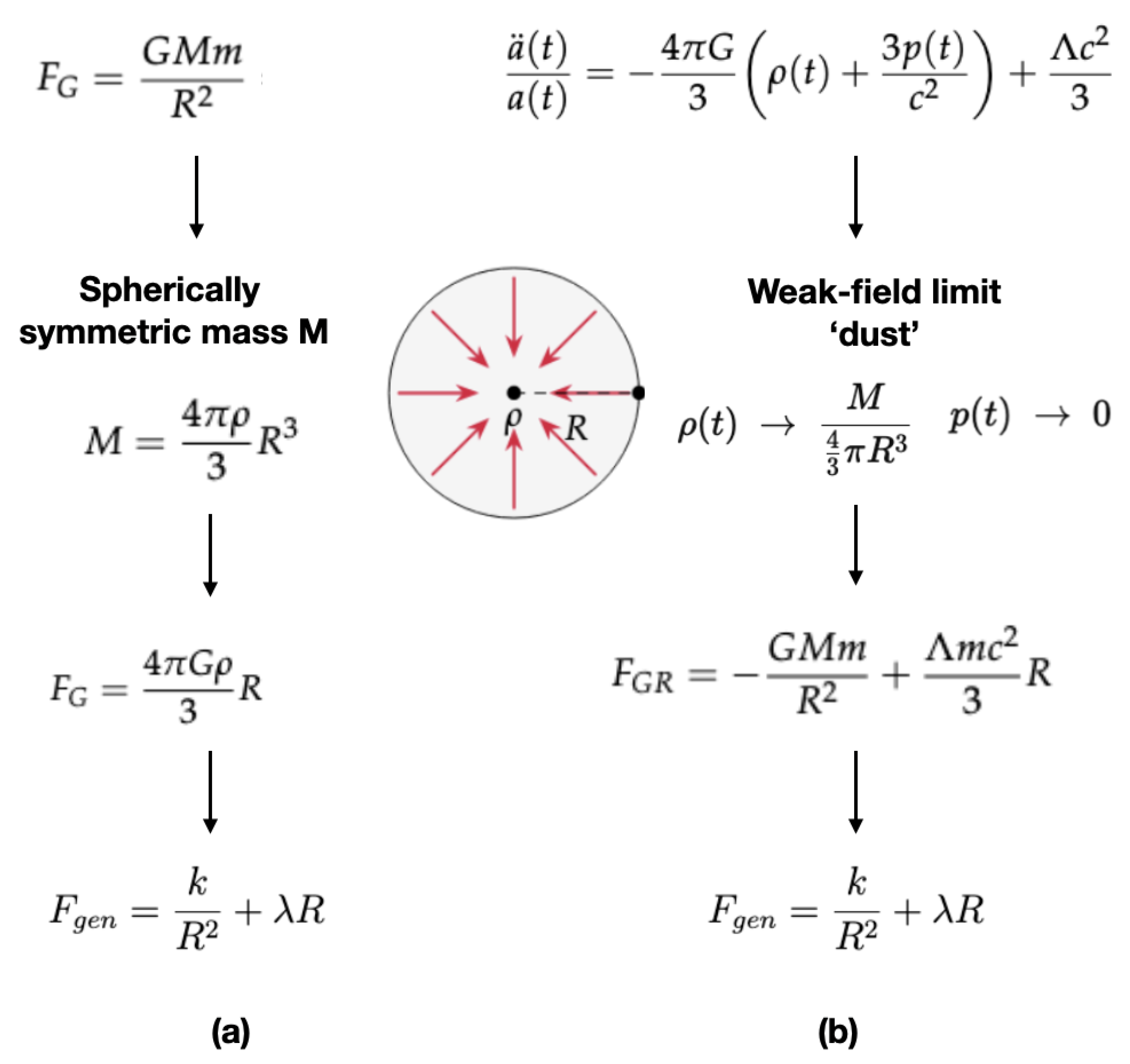
Table 1.
Thermodynamic properties of three causal horizons. All obey the universal relations and area. For the Rindler horizon we report entropy per unit transverse area (as in Figure 3); for Schwarzschild and de Sitter we use the total area A. They differ only in how the effective radius R is set: by proper acceleration (, Rindler), by mass (, Schwarzschild), or by the vacuum (, de Sitter).
| Spacetime | Horizon Type | Horizon Radius R | Temperature T | Entropy S |
|---|---|---|---|---|
| Rindler | Acceleration | observer-dependent | ||
| Schwarzschild | Event Horizon | |||
| de Sitter | Cosmological |
Table 2.
Comparison of force quanta in Stoney, Planck, and units. In the -framework, all force quanta are scaled relative to the entropy-bound limit.
Table 2.
Comparison of force quanta in Stoney, Planck, and units. In the -framework, all force quanta are scaled relative to the entropy-bound limit.
| Force Type | Stoney Units | Planck Units | Lambda Units |
|---|---|---|---|
| Inertial | |||
| Gravitational | |||
| Electromagnetic |
Table 3.
Comparison of Planck and natural unit systems. Planck units arise by heuristic dimensional analysis of , while -units are fixed by the thermodynamics of causal horizons (Bekenstein–Hawking, Gibbons–Hawking), embedding entropy intrinsically and uniquely reproducing the GR vacuum energy density.
| Feature | Planck System () | System () |
|---|---|---|
| Core base units | Length , Time , Mass . | Length , Time , Mass . |
| Method of derivation | Heuristic dimensional analysis of . Unique by construction but thermodynamically sterile. | Thermodynamics of causal horizons (Bekenstein–Hawking, Gibbons–Hawking). Vacuum energy density uniquely fixed, with entropy intrinsic. |
| Role of | Present in Planck’s original set but drops out of . Thermodynamics not built-in. Temperature only via a bolt-on Planck temperature. | Thermodynamics embedded in base units . The Bekenstein–Hawking relation gives a fundamental entropy unit . |
|
Entropy/ thermodynamics |
Absent from core units. No natural unit of entropy. Essentially a mechanical system. | Entropy is intrinsic. Causal horizons saturate a finite entropy bound, embedding thermodynamics at the foundation. |
| Cosmological constant | Assumes (relic of a non-accelerating cosmos). No scale associated with vacuum energy. | fundamental. Uniquely fixes the vacuum energy density , linking quantum and thermodynamic structure. |
Disclaimer/Publisher’s Note: The statements, opinions and data contained in all publications are solely those of the individual author(s) and contributor(s) and not of MDPI and/or the editor(s). MDPI and/or the editor(s) disclaim responsibility for any injury to people or property resulting from any ideas, methods, instructions or products referred to in the content. |
© 2025 by the authors. Licensee MDPI, Basel, Switzerland. This article is an open access article distributed under the terms and conditions of the Creative Commons Attribution (CC BY) license (http://creativecommons.org/licenses/by/4.0/).
Copyright: This open access article is published under a Creative Commons CC BY 4.0 license, which permit the free download, distribution, and reuse, provided that the author and preprint are cited in any reuse.


