
Submitted:
27 October 2025
Posted:
28 October 2025
You are already at the latest version
Abstract
The risk-return relationship has been a fundamental concept in finance, highlighting the trade-off between potential gains and the likelihood of losses. There are various model to establish the risk return relationship such as CAPM, French and Fama three factors and five factors models, etc. However, these traditional models assume a constant risk-return relationship, which may not capture the dynamic nature of financial markets. This study aims to explore the fitting and forecast gain of employing time-varying approaches in analysing the risk-return relationship. Alternative modelling techniques including Rolling Regression models, Markov-switching models, and Kalma filter-based state-space models to investigate the time-varying nature of risk and return relationship. These techniques allow for the estimation of varying risk and return parameters across different market conditions and economic regimes. The empirical investigation reveals that the risk-return relationship is not constant over time, suggesting the presence of market fluctuations. By accounting for these variations, investors and policymakers can make more informed decisions regarding asset allocation, risk management, and investment strategies, and emphasize the significance of employing time-varying approaches in analysing the risk-return relationship. The findings have implications for portfolio managers, policymakers, and investors.
Keywords:
risk-return relationship
; time-varying approaches
; rolling models
; markov-switching models
; state-space models
1. Introduction
The rewards from investing in stocks can be volatile and hard to predict. The rate of return that investors anticipate from their investments also varies with market volatility and uncertainty. When analysing stock market behaviour, conventional wisdom holds that investors always have the same expectations and that certain metrics, like as “beta,” which indicates how a stock’s price changes in relation to the entire market, remain stable throughout time.
But in reality, the risk of an investment might shift for a variety of reasons, both great and minor. Therefore, we have seen that beta, which indicates risk related to market fluctuations, can shift over time for various assets. The beta of an investment tells us how risky it is relative to the market as a whole. It tells us how sensitive the stock price is to market-wide fluctuations. Beta is crucial since it reveals the amount of risk that cannot be mitigated by diversifying holdings. (Sharpe, 1970).
There has always been controversy about the model setting and statistical test of market beta estimation in finance. Most of the studies, like Roll (1977) and Shanken (1985), estimate market beta by means of the ordinary least squares (OLS) estimation technique, expecting that beta will be steady after some time. Some other studies have shown that there are some problems with using a method called “time-rolling OLS” to predict how beta values change. This method is used to figure out how beta changes over time, but it may not be very exact and may not show how beta really changes. Several researchers have written about these issues, including Bollerslev et al. (1988), Hentschel (1992), Glosten et al. (1993), Fabozzi and Francis (1978), Bos and Newbold (1984), and others. They have pointed out the problems with using time-rolling OLS to estimate beta values that change over time and how to work around them.
Things are constantly changing in the actual world, and the risk of investments (represented by beta) can fluctuate over time. This means that a stock’s beta is dependent on the information available at a given time and can increase or decrease as circumstances change.Cash flow fluctuations can affect a company’s beta, which assesses its risk in relation to the overall market, according to experts. These fluctuations frequently occur during business cycles, also known as economic ups and downs. Business cycles are influenced by factors such as technological advances and changes in consumer preferences, which have varying effects on various economic sectors. As a result, the beta of equities in these industries can increase or decrease proportionally (Jagannathan and Wang, 1996). While many studies have examined whether beta remains constant as a result the explicit modelling of how systematic risk changes over time has received less attention especially in the case of emerging economies. In this study, we will employ a variety of techniques, including rolling regression, regime switching State Space model-based Kalman filter approaches, to examine and comprehend how the beta of various sectors fluctuates over time.
Predicting how beta changes over time is important because it tells us if a trade is riskier or more stable than the market as a whole. Beta measures the risk that comes from changes in the market as a whole, which cannot be lessened by spreading your investments out (Sharpe, 1970). Financial managers in corporations find that beta change over time are helpful when making decisions about their company’s capital structure and evaluating investments. Scholars focus on testing how beta changes over time because it is one of the most important ways to measure the regular risk of an investment’s return. Financial economists and practitioners use beta to estimate stock sensitivity to the overall market, identify mispricing of shares, and apply evaluation models and performance evaluation. In Pakistan’s context, research on time varying is perhaps a novel concept. Therefore, this study aims to fill this literature gap and uses different techniques to model and estimate the time-varying betas in important sectors on the Pakistan Stock Exchange (PSE). Thus, the aim of this study is to examine the time-varying nature of beta on the Pakistan Stock Exchange (PSE) at sector level. Our main goal in writing this article is as follows:
- Our research seeks to investigate the beta parameter, particularly time-varying beta, on the Pakistan Stock Exchange (PSX), one of the largest emerging financial markets in South Asia.
- In addition, we will develop and employ three distinct econometric techniques, namely rolling, regime switching, and the Kalman filter method, to estimate beta parameters that vary with time. Notably, such sector-level analyses have never been conducted for the PSX.
- Finally evaluate the performance of different estimation techniques in capturing systematic risk and forecasting sector returns. To achieve this objective, the effectiveness of these techniques will be assessed using several information criteria, including mean average error (MAE), mean squared error (MSE), and model confidence set (MCS). By employing these criteria, the study aims to identify the best estimation technique that outperform the others in terms of accuracy and reliability in predicting sector returns and capturing movements in systematic risk.
We analysed time-series datasets for 13 designated Pakistan Stock Exchange (PSX) industry sectors. We compared the result with beta estimates derived from Sharpe’s linear Capital Asset Pricing Model (CAPM) and the three-factor model, which served as benchmarks. We estimated beta parameters using the maximum likelihood method using monthly data from 1995 to 2021. Our analysis involved ranking the various estimation techniques according to three criteria (MAE, MSE, and MCS) of fit and investigating correlation coefficients between the results. The empirical findings of our study raised important challenges when using the single-factor CAPM and the three-factor model for the 13 sector of the Pakistan Stock Exchange. Pakistan’s sector betas exhibited high volatility over time, indicating that time-varying beta estimates are more suitable for constructing low-risk portfolios and accurate long-term forecasting. In comparison to other time-varying techniques, such as rolling and regime switching, and standard econometric techniques such as Ordinary Least Squares (OLS), the Kalman filter approach proved to be the most advantageous. The Kalman filter method proved efficient for monitoring structural changes in systematic risk and estimating beta parameters in emerging markets. It is essential to observe that only a handful of studies have examined the stochastic process of beta variation on the Pakistan stock exchange. Our research is the first major investigation in this field.
The rest of paper is structured as follows: Section 2 introduces existing literature from both international and local markets on the measurement of the asset pricing model. Section 3 presents the various non-parametric approaches for estimating the time-varying beta coefficient. In this section, we analyse the static properties of three non-parametric estimation methods. Before discussing the main result, an overview of the data and summary state will be presented in Section 4. The main result will be discussed in Section 5, and model comparison test is presented in section 6. Finally the conclusion is discussed in section 7.
2. Review of Literature
This section provides a comprehensive overview of existing research and studies related to the estimation and modelling of beta parameters in the context of stock markets. This section is divided into two main sections, namely literature related to Pakistan (Section 2.2.1) in which i focuses on studies conducted specifically in the context of Pakistan stock market and literature related to international studies (Section 2.2.2) where the literature review expands beyond the Pakistani context and investigates into studies conducted in international markets.
2.1. Studies from International Markets
The development of the Capital Asset Pricing Model (CAPM) is attributed to prominent scholars such as Sharpe (1964), Lintner (1965), and Markowitz (1996). CAPM is a widely recognised and utilised framework for evaluating the worth of various assets. The Capital Asset Pricing Model (CAPM) posits that the anticipated surplus return of an asset is contingent upon its responsiveness to fluctuations in the broader market. The quantification of this sensitivity is achieved by the use of the asset’s beta coefficient, which is afterwards multiplied by the market risk premium. The beta coefficient quantifies the historical correlation between the asset’s returns and the returns of a market portfolio. The metric functions as an indicator of the asset’s systematic risk, encompassing the asset’s tendency to fluctuate in relation to the broader market. A beta value over 1 denotes that the asset exhibits more volatility in comparison to the overall market, whilst a beta value below 1 shows relatively lesser volatility when compared to the market. A beta value of 1 indicates that the asset exhibits a correlation with the market, meaning it moves in tandem with market movements. Historically, it has been conventionally considered that beta remains unchanged throughout time, so suggesting a consistent association between the returns of an asset and the returns of the market. Nevertheless, it should be noted that in practise, the value of beta is not always constant, but rather subject to variability in response to various market situations.
But the CAPM has been criticised by experts like Black, Jensen, and Scholes (1972), Fama and French (1992), and Fama and MacBeth (1973). They say that using just one factor, like market beta, is not enough to show the full systemic risk of a product. Other improvements to the basic CAPM have focused on adopting more flexible estimation approaches in which the beta coefficients are not assumed to remain constant throughout time or place. Fama and French (1997, 2006) The single index model is used by Schwert and Seguin (1990) to account for the time-varying heteroscedasticity of portfolio returns that is dependent on business size. This model calculates the time-varying beta as part of the portfolio volatility prediction process. A Kalman filter model based on state space is naturally suited to estimating time-varying betas in a dynamic system, and it has been utilized in several studies to do so (e.g., Black et al., 1992; Wells, 1995). Although all strategies reflect the characteristics of time-varying systematic risk, there is no clear winner when it comes to predicting systematic hazards. Some research has compared the Kalman filter method’s predicting ability to that of GARCH-based models and other estimate approaches (Faff et al., 2000; Choudhry and Wu, 2008; Mamaysky et al., 2008).
Conversely, the beta values of equities may demonstrate volatility as a result of many factors. Market dynamics is a crucial aspect that contributes significantly to the observed volatility. When a firm modifies its business strategy or capital structure, these adjustments can have a significant impact on its returns and, consequently, its beta coefficient. Furthermore, it is worth noting that microeconomic factors, such as a firm’s dividend policy or the level of financial leverage it utilises, might exert an influence on beta in the long run. Various empirical investigations conducted in different financial markets, such as the American market (Fabozzi and Francis, 1978) and the European market (Wells, 1995; Chaveau and Maillet, 1998), have shed light on the possibility of beta fluctuation across time. These studies provide evidence that swings in beta values may be attributed to changes in market and microeconomic variables.
French (2016) looked at the Capital Asset Pricing Model (CAPM) betas for five ASEAN nations and US industries in one recent study. He contrasted conventional constant beta models with time-varying beta models. The findings demonstrated that when assessing the mean-square error threshold, the Kalman Filter method using a random walk parameterization outperformed alternative models. It follows that combining these strategies might result in more accurate methods for calculating how beta changes over time.
Research on global CAPM time-varying betas for Asian and Japanese stock returns was done by Tsuji (2017). He discovered that the time-invariant international CAPM beta of the North American and European equities portfolios were similarly calculated using the traditional ordinary least squares (OLS) approach. The worldwide CAPM betas of North American equities portfolios, however, varied with time, being slightly greater before 1996 and significantly smaller after 1996.
Elshqirat and Sharifzadeh (2018) looked into the returns on Jordanian stocks. Their findings demonstrated that neither market return nor firm size nor financial leverage could predict the projected rate of return. They might foresee operating leverage, nevertheless. Using the CAPM, FF3 model, and FF5 model, Sundqvist (2017) examined average returns in the Nordic markets from December 1997 to June 2016. He explains the average returns of portfolios ordered by size and investment and by size and book-to-market ratio, but not those of portfolios sorted by size and profitability. His result shows that the FF5 model performs well for Nordic markets as compared to the rest of the other models. Using average stock returns for developing and certain established equity markets from January 2010 to December 2015, Mosoeu and Kodongo (2019) estimate the parameters of a five-factor model by applying the Generalized Method of Moments (GMM). Their results show that RMW (the difference between the returns on portfolios with robust profitability and portfolios with weak profitability) is the most useful model for describing equity returns in developing markets.
However, the outcomes of numerous other studies do not match those of the ones mentioned above. Using the CAPM, FF3 model, and four-factor model, Nguyen (2016) examined the stock market’s average return in Vietnam from January 2011 to December 2015. His findings demonstrate that the R-square rises steadily from the CAPM to the four factor model, with the four factor model having the greatest R-square, albeit at only 34%, with RMW and CMA being irrelevant in explaining stock returns. These results are similar to the work by Kubota and The study done by Takehara (2018) utilised the Generalised Method of Moments to evaluate the effectiveness of the Fama-French Five-Factor (FF5) model in elucidating stock returns on the Tokyo Stock Exchange (TSE) over the period spanning from January 1978 to December 2014. The research findings revealed that the variables RMW (Robust Minus Weak) and CMA (Conservative Minus Aggressive) had a restricted capacity to explain stock returns. Therefore, the authors reached the conclusion that the initial FF5 model was unsuitable as a benchmark pricing model for Japanese stocks. In an unrelated context, Wijaya, Irawan, and Mahadwartha (2018) utilised the FF5 model to analyse the performance of firms included in the LQ45 Index over the timeframe spanning from January 2013 to December 2015. The researchers noted in their analysis that the variable of risk management practises (RMW) did not have a statistically significant influence on investment returns. Nevertheless, the researchers discovered that the market risk premium (Rm-Rf), the High Minus Low (HML) factor, and the profitability factor (CMA) had considerable positive impacts on investment returns. Conversely, both the HML and CMA factors were found to have large adverse effects on returns. These two research papers offer significant contributions to understanding the suitability of the FF5 model in various market scenarios. The results emphasise the significance of taking into account the unique characteristics and dynamics of local markets when using pricing models for the analysis of stock returns. This emphasises the need of meticulously customising pricing models to suit particular market situations and the distinct elements that influence stock returns in various areas and timeframes.
The study conducted by Chiah, Chai, Zhong, and Li (2016) aimed to examine the suitability of several asset pricing models in relation to the Australian stock market throughout the timeframe spanning from January 1982 to December 2013. The researchers’ investigation unveiled that the five-factor model, as posited by Fama and French, exhibited a heightened capacity to elucidate a wider array of anomalies in asset prices in comparison to the other asset pricing models that were studied. This discovery provides substantial evidence to substantiate the efficacy and pre-eminence of the five-factor model within the framework of the Australian stock market. Additionally, the researchers utilised the GARCH (Generalised Autoregressive Conditional Heteroscedasticity) model in order to effectively forecast the volatility of equities. The GARCH model is widely recognised for its ability to effectively capture and predict the dynamic nature of volatility in financial asset returns. Through the use of this methodology, Chiah et al. successfully attained accurate forecasts of stock volatility, therefore augmenting the comprehension of risk dynamics inside the Australian stock market. Using artificial neural networks, Jan and Ayub (2019) predicted stock returns in developing economies. Their research supports the adage in finance that “high risk leads to high return,” and the FF5 model based on stock returns in developing economies will greatly boost returns on investments.
2.2. Studies from the Pakistan Stock Exchange Market
In general, there are several methods for estimating beta parameters in established markets, with the Kalman filter technique being one of the most effective methods for estimating time-varying beta values. Nonetheless, there remains a research gap in the growing markets of South Asia. The first study in this field was undertaken by Taufiq Choudhry, Lin Lu, and Ke Peng (2010), who used daily data to look at the four Asian sector indexes. They used the bivariate MA-GARCH model (BEKK) to provide a better picture of evolving assumptions about systemic risk. Their results show that the Asian financial crisis and the time after it had an effect on how the industrial betas of these countries changed over time, and these results could mean something for investors who are interested in managing the risk of their portfolios.
The second research, done by Gagari Chakrabarti and Ria Das (2021), looked at modelling time-varying systematic risk in the comparison between India and the American capital markets from 1999 to 2017. The author used MA-MGARCH model specifications to compute beta. Researchers discovered a significant relationship between time-varying betas and local market volatility in both nations. When the local market was under pressure, developing markets’ betas increased.
In a 2007 study, Iqbal and Brooks examined the conditional Fama-French three-factor model and the CAPM for stocks traded on the KSE-Pakistan. For 89 stocks, they used data from 1992 to 2006. They found that conditioning factors frequently resulted in an upward bias by applying GARCH and EGARCH algorithms on monthly, weekly, and daily data. Finally, they came to the conclusion that the unconditional three-factor model was superior. Mirza and Shahid (2008) used a multivariate framework to examine the reliability of the three-factor model for 81 stocks traded on the Korean Stock Exchange (KSE) between January 2003 and December 2007. They found a value discount in their data, which generally supported the three-factor model even though they validated the size premium.
The market risk premium and a set of macroeconomic factors were examined by Javid and Ahmad (2008) for 49 stocks that traded on the KSE between 1993 and 2004. Their conclusions suggested that economic factors had little bearing on stock return volatility and that this variability had some relationship to business cycles. Every publication in the review of the literature employed different asset pricing models, which are based on multiple linear regression models with time-invariant parameters; hence, those models are unable to capture and display a varied effect for the different elements at various periods. By this time, is it interesting to explore whether we can capture and demonstrate a distinct effect for different elements at various periods or not?
3. Methodology
This section presents the approach and techniques employed in this study to estimate and model beta parameters in the context of the Pakistani sector market. In section 3.1 we introduces the OLS technique, a widely used econometric approach for estimating beta parameters. It provides an overview of the underlying assumptions and procedures involved in OLS estimation. The rolling regression approach is discussed in section 3.2. It explains the concept of rolling windows and how they are applied to estimate beta parameters over successive time intervals. The regime switching technique is introduce in section 3.3 which allows for the estimation of beta parameters under different market regimes or states. Finally the state space model is discussed in section 3.4 which discusses the concept of state space representation and the use of Kalman filter-based approaches like RW, AR and VAR.
3.1. Unconditional Constant Coefficient Within the CAPM Model
The predicted return on a particular sector (i) is closely correlated with its systematic risk, which is represented by beta, in the Sharpe and Lintner (1969) CAPM model. When investors have the choice of borrowing or lending money at a risk-free interest rate, this relationship still holds true.
where represents the return on sector i, represents the return on market portfolio, and represents the risk-free rate of return, respectively. In this context, the predicted CAPM risk premium of an asset is used to explain the asset’s excess return, denoted by the notation . Jensen’s alpha refers to the intercept coefficient , and it is defined as having a value of zero for each asset (Jensen 1968), which treats systematic risk as if it were always there and uses this assumption to derive estimates of constant betas.
In this case, an asset’s predicted CAPM risk premium is used to figure out its excess return. The intercept parameter, also called “Jensen’s alpha,” is set to zero for each asset, as suggested (Jensen, 1968). The ordinary least squares (OLS) method is used to predict constant betas in the standard market model, which assumes that systematic risk is always the same.
Where is likely to be zero and is the systematic risk of sector against the market portfolio, with
The error term is assumed to be independently and identically distributed and to have a zero mean and a constant variance for sector .
Now, adding two more factors (SMB and HML) to Fama and French’s three-factor model and adding the above equation, the model can be written in a general form as
3.2. Time Varying Co-Efficient with the Rolling OLS Beta Model
The recursive OLS estimation of the market model is a simplest way to get estimates of betas that change over time. Fama and MacBeth were the first to use this method (1973). In this process, the minimization of a local sum of squared residuals for each portfolio can be written as
Where r shows how many past observations should be taken into account at each estimation point. The rolling OLS estimator can be found by looking at the first-order conditions of the optimization problem as
Where is the observation of the data matrix and subscript ROLL is the OLS rolling estimator. When this estimator is used in the real world, a window of 60 observations is used for monthly data. The number of samples is chosen based on the findings of Bollerslev and Zhang (2003) and Ghysels and Jacquier (2006).
3.3. Time Varying Co-Efficient with in Markov Switching Dynamic Regression Model
The Markov switching approach also belongs to the class of state space models. The Markov switching approach, specifically, is a type of state space model where the system is assumed to switch between different regimes or states. Each regime represents a different set of parameters or dynamics that govern the generation of the observed data. The transitions between these regimes are assumed to follow a Markov process, meaning that the probability of switching from one regime to another only depends on the current regime. The implicit assumption underlying Markov switching models is that the observed data result from a process that undergoes abrupt changes or shifts between different regimes. These shifts can be caused by various factors such as political events, economic shocks, environmental changes, or other exogenous influences. The Markov switching approach allows for the modelling of these regime changes and provides a framework to estimate the probabilities of being in each regime and the associated parameters. For a model with two states, the following regimes Markov-switching model can be written:
.
Where could be state 1 to state n regimes
and
denote the conditional alpha and beta in each state.
3.4. Time Varying Co-Efficient with State Space Model
The state space representation of a model is necessary for the Kalman filter method of estimating the time-varying beta parameter. A measurement equation and a transition equation make up the state space form. The transition equation shows how the beta parameter changes over time while the measurement equation specifies the relationship between the observable variables (such as stock returns) and the unobserved state variable. By revising the forecast of the beta parameter at each time step based on the observed data and previous estimates, the Kalman filter technique uses a recursive algorithm to estimate the beta parameter. The observation equation and the state equation in our work can be used to explain the Kalman filter equations as
To simulate a range of in the literature identified specifications of systematic risk behaviour, we use various time-varying beta models as a state equation. The AR model is one definition for a time-varying beta model. The time-varying beta is assumed to be an autoregressive stochastic process with an autoregressive parameter that reflects the shock’s persistence. If the shock’s persistence is near to 1, the shock will have an effect on the beta in following periods. A number that approaches 0 indicates that the shock has little effect on the beta in subsequent periods. The equation (1) is represented in the AR format as
Another important time-varying coefficient model is the RW model. In the RW format the equation (2) is written as
In this specification, it is assumed that the sector model’s alpha and beta parameters follow stochastic and Gaussian random walks and are time-varying (i.e., not constant over time). The stability of the stochastic sector alpha and sector beta parameters is determined by the parameters utilised in this equation. Less volatility is permitted and the time-varying parameter becomes more stable as the variance of the state error component declines. Constant sector parameters are achieved in this exceptional instance when the variance goes to zero. On the other hand, as the variance rises, the stochastic parameter’s present state could diverge significantly from its previous state.
The third version of the state space model suggested by Cogley and Sargent (2001, 2005) and Primiceri (2005) assumes that the time-varying beta is a VAR process with a vector autoregressive parameter. In the VAR format, the equation (3) is written as
4. Data, Variables Construction and Summary States
This section of study provides a comprehensive overview of the data, variables construction and summary statistics. Section 2.4.1, describe the data sources and characteristics in detail. The construction and selection of variables used in the estimation is discussed in Section 2.4.2. Finally the section 2.4.3 provides a summary of key statistical measures calculated from the dataset.
4.1. Data Explanation
This paper intends to investigate the time-varying beta of 13 industries classified by the Stock Exchange of Pakistan (PSX) over the period February 1995 to August 2021, a total of 320 observations (320 months in all). The range of the data that is obtained from the data stream database [1] depends on the availability of all variables that are used for the construction of portfolios. To get rid of the noise in the daily and weekly returns, we take the monthly data for the sector return. The data on monthly factor returns for Market (MKT), Size (SMB), and Book-to-Market (HML) come from the same database. The 6-month government bond yield is used as a stand-in for the risk-free interest rate.
4.2. Variables Construction
The return of each industry portfolio is the dependent variable in this study, whereas the market factor, the size factor, and the value factor are the independent factors. The market component is identified in both the CAPM and the Fama-French three-factor models by calculating the discrepancy between the return on the market portfolio and the risk-free rate. Size-value is utilised to build six portfolios in the Fama-French three-factor model (Fama and French, 1992). The average return on three small portfolios (SL, SM, and SH) less the average return on three large portfolios (BL, BM, and BH) equals the size premium (SMB). The average return on two value portfolios (SH and BH) minus the average return on two growth portfolios (SL and BL) is known as high minus low (HML).
and are computed as follows:
4.3. Summary States
In Table 1, we can see how the monthly returns for different industries are spread out. The average monthly return is about 0.013 percent, which is the same as 13% per year. The oil and gas, auto, and beverage industries had the highest returns, averaging between 12 and 18% per year, while several other industries had average returns as low as 7% per year. As we might expect, there is a fairly strong link between the number of companies in an industry and the total risk of that industry, which is measured by the standard deviation. As a measure of risk, the standard deviation goes from the low-risk pharmaceutical sector (0.087) to the high-risk Travel and Leisure and Electrical sectors (0.123 and 0.114, respectively). There is an excess kurtosis that is more than the typical value of zero for all sectors, factors, and the market. This indicates that huge outliers occur more frequently than we would anticipate if everything else were normal since all excess returns and variables are more concentrated around the mean (leptokurtic). Except for market returns, the risk-free rate, and variables like SMB, all sectors are adversely skewed, according to the skewness data. This could mean that large positive returns happen more often than large negative returns. Harvey and Siddique (1999) point out that the Pakistan Stock Exchange (PSX) is different from some developed and emerging markets. Table 1 also shows the autocorrelation series at points Q (1), Q (3), Q (6), and Q (12) for each sector’s excess returns, market returns, and factors. The autocorrelation value is lowest for the market return at points Q (1) and Q(12), and it is highest for the risk-free rate at points Q(1) and Q(12). The Jarque-Bera statistic rejects the null hypothesis that all series are normal. This means that there may be nonlinear patterns in the way monthly return series change over time. Lastly, the ADF-test statistics show that all market returns, factors, and sector returns are level across all industries.
5. Result Interpretation
This section provides a comprehensive analysis and interpretation of the findings obtained from the estimation and modelling of beta parameters using different techniques in the Pakistani sector market. The section is structured into four subsections, each focusing on the results derived from specific estimation methods. Section 1 presents the results obtained from the Ordinary Least Squares (OLS) estimation technique. The results from the rolling regression technique are presented and analysed in section 2. The findings derived from the regime switching estimation technique is presented in section 3. Finally the results from the state space models, including specific estimation methods such as RW, AR, and VAR are presented and analysed in section 4.
5.1. Ordinary Least Square (OLS) Estimates
In this section, we analyse the standard CAPM and the Fama-French three-factor model by employing time-series regression for each of the industrial sector returns. The objective of this approach is to identify the role of size and value factors in capturing variation in stock returns during the period from February 1995 to August 2021. We start with the traditional single-factor CAPM in order to make a comparison with the three-factor model later. The results reported in Table 2 show that the average adjusted value of the CAPM is approximately 43%, suggesting that the CAPM does not explain most of the time-series variations in industry stock returns. The intercept of the CAPM is statistically significant for 11 out of 13 industry sector portfolios.
Next, we include size and book-to-market factors into the model, and
Table 2 reports the results of the Fama-French three-factor model. The 13 industry sector regressions, with an average of approximately 49.48%, are higher than those of the CAPM regressions. Usually, adding an independent factor to regression increases If the change is meaningfully higher, it is considered an improvement in the model. The average value of industry sector return increases from approximately 26.18% to 70.48%, signifying that the three-factor model provides a massive improvement in the explanatory power over the CAPM. Therefore, our regression results support the argument that the three-factor model is a much better fit for the Pakistan Stock Exchange (PSX) at the industry sector level.
Theoretically, if a model satisfactorily explains the changes in the expected returns, then the intercept produced by regression results will tend towards zero.
Table 2 reports that the 13 industrial sector portfolios produce intercepts ranging from 0.019 to 0.094, which are close to zero. Few industrial sector portfolios (like Chemical, minerals, and mining; electrical; telecommunication; and Travel and leisure) show a significant (negative) intercept. The significant intercept for these industries portfolios indicates that the firms have something not predicted by the model. The loadings on the market factor are all significant at the 1% level and thus reflect a positive return from it.
Sensitivity to market risk, that is, HML, has significantly positive coefficients for the majority of the industrial sector and significantly negative coefficients for a few industrial sectors. Similarly, the coefficients of most of the industrial sectors have both negative and positive sensitivity to SMB, and a few industrial sectors have insignificant sensitivity. The coefficients of the industrial sector range from approximately 0.007 to 0.284. This finding also indicates adequate evidence to support the existence of a size premium in the model.
5.2. Rolling Regression Estimates
The estimation of time series beta coefficients using the rolling regression OLS technique revealed interesting findings. We used a window size of 60 months and a selected bandwidth of 1 for each of the 13 sectors with available data for the entire sample period. To ensure consistency, the rolling-regression betas for the first 60 months were set equal to their value for the 60th month, which was the first period for which the betas were estimated.
The results of the rolling regression analysis indicated that the one-month sub-period betas exhibited substantial fluctuations over time, indicating the instability of betas for both the CAPM and Three Factor Model. The estimated betas showed significant changes from one period to the next, suggesting the presence of intertemporal instability. These findings align with the statistical evidence presented in Table 3 and Figure 1 and Figure 2.
Figure 1 shows time-varying beta coefficients for the CAPM estimates across different sectors. In the Auto sector, the beta coefficient fluctuates around 0.85 to 1.03 over the observed period, indicating that the sensitivity of Auto companies’ returns to market movements varied but generally stayed close to the market. For the General Industries sector, the beta ranges between approximately 0.92 and 1.05, reflecting a similar pattern of moderate sensitivity to the market. In the Oil and Gas sector, the beta spans from around 0.94 to 1.11, suggesting a wider range of sensitivities, possibly due to factors such as oil price volatility and geopolitical events. Overall, the varying beta coefficients highlight the dynamic nature of these sectors’ risk profiles in response to changing market conditions over time.
Figure 2 shows represents the sensitivity of a stock’s returns to changes in the overall market returns and other two factors. It is a measure of how much a stock’s returns tend to move in response to three factors. A beta value greater than 1 indicates that the stock is expected to be more volatile than the market, while a beta value less than 1 suggests lower volatility compared to the market. The beta values for different categories within the Auto sector change over time. This indicates that the sensitivity of the returns of companies in the Auto sector to market movements is not constant and varies from month to month. Similar to the Auto sector, the beta values for different categories within the General Industry sector also change over time. This implies that the sensitivity of the returns of companies in the General Industry sector to market fluctuations is not consistent. Finally the beta values for different categories within the Oil and Gas sector also exhibit time-varying behaviour. This sector’s beta values can be influenced by factors such as oil prices, geopolitical events, and changes in energy demand.
These findings are consistent with previous research that has highlighted the instability of beta estimates over time. For instance, Tsuji (2017) found similar results in their study, stating that “beta estimates tend to vary widely over time, indicating the dynamic nature of systematic risk. Another study by Yeo (2004) also supported this notion, stating that the rolling regression approach allows for capturing the time-varying behaviour of beta, revealing significant fluctuations and highlighting the instability of betas over different time periods.
Despite the observed instability, the equations reported in Table 3 demonstrated good explanatory power, with most sectors in both models exceeding 50% explanatory power and only a few sectors have less than 50 percent reported. This suggests that the chosen regressors effectively capture the variation in sector returns. The regressors are significant, the intercept is significant and positive in all cases, and the trend term is significant in the equations for all of the sectors and is also positive.
5.3. Regime Switching Estimates
The Table 4 and Table 5 explores a two-state model that identifies two different regimes in the dependent variable, which is the expected return exposure on Pakistan’s industry. The model assumes that the dependent variable follows a mixed normal distribution with two constant regime-dependent expected returns and volatilities. The findings of the study reveal that the regime-switching model has divided the data into two distinct regimes that is one with a low mean (referred to as the low exposure regime) and the other with a high mean (known as the high exposure regime). This distinction was observed across all industries analysed in the study. During the low exposure regime, the anticipated monthly mean of conditional sector beta (a measure of sensitivity to market movements) ranged from 0.89 to 1.16, while during the high exposure regime, it ranged from 0.94 to 1.31. It was also noted that few industries had betas value below 0.80 during the low exposure regime, while none of the industries had betas is less than 0.80 during the high exposure regime. While in Table 5, we found that during the low exposure regime, the anticipated monthly mean of conditional sector beta (a measure of sensitivity to market movements) ranged from 0.04 to 1.72, while during the high exposure regime, it ranged from 0.11 to 1.98.
The Table 4 and Table 5 further examined the volatility levels in each state, represented by sigma coefficients. Generally, it was found that regime 1 (low exposure) had higher volatility than regime 2 (high exposure) for most industries, except for the food, mineral, personal goods, and travel and leisure sectors. These sigma values that differ from zero indicate that sector volatilities are regime-dependent. The estimated transition probabilities, specifically p11 (0.91) and p22 (0.83), provide insights into the likelihood of transitioning between states. For example, in the auto sector, if it is currently in the low exposure state (state 1), there is a 91.19% probability that it will remain in that state during the following month. Similarly, there is only a 0.83% probability that the market will switch to the high exposure state (state 2) next month. These transition probabilities indicate that either of the two states is highly persistent.
Table 6 and Table 7 calculated the duration of each state, which represents the time the time-varying beta remains in a given state. The duration for remaining in state 1 (low exposure) was approximately 124 months, while for state 2 (high exposure), it was around 104 months. This further supports the observation that the regimes are persistent in most sectors.

Table 6.
Estimation of transition probabilities for CAPM model.
| Duration | Auto | Beverages | Chemical | Chemical and Mining | Electrical | Food | General Industries | Minerals | Oil and Gas | Personal Goods | Pharmasutical | Telecommuniction | Traavel and Leisure |
|---|---|---|---|---|---|---|---|---|---|---|---|---|---|
| State 1 | 112.67 | 115.42 | 106.51 | 55.66 | 66.94 | 42.71 | 131.33 | 33.77 | 131.01 | 104.07 | 101.43 | 11.18 | 71.21 |
| State 2 | 98.59 | 221.22 | 88.18 | 48.53 | 55.20 | 38.41 | 224.06 | 28.36 | 142.51 | 98.33 | 156.32 | 4.03 | 65.72 |
| Percentage in Stage 1 | 53.33 | 34.29 | 54.71 | 53.42 | 54.81 | 52.64 | 36.95 | 54.36 | 47.90 | 51.42 | 39.35 | 73.50 | 52.00 |
| Percentage in Stage 2 | 46.67 | 65.71 | 45.29 | 46.58 | 45.19 | 47.36 | 63.05 | 45.64 | 52.10 | 48.58 | 60.65 | 26.50 | 48.00 |
Note: The table presents the estimation of transition probabilities for the Capital Asset Pricing Model (CAPM) model. The two states in focus are state 1 and state 2. State 1 represents the duration of being in state 1, while state 2 represents the duration of being in state 2. The transition probabilities are indicated by percentage 1 and percentage 2, which show the probabilities of transitioning between state 1 and state 2. Percentage 1 represents the probability of moving from state 1 to state 2, while percentage 2 represents the probability of moving from state 2 to state 1.
Table 7.
Estimation of transition probabilities for three factor model.
| Duration | Auto | Beverages | Chemical | Chemical and Mining | Electrical | Food | General Industries | Minerals | Oil and Gas | Personal Goods | Pharmasutical | Telecommuniction | Traavel and Leisure |
|---|---|---|---|---|---|---|---|---|---|---|---|---|---|
| State 1 | 112.67 | 115.42 | 106.51 | 55.66 | 66.94 | 42.7 | 131.33 | 33.77 | 131.01 | 104.07 | 101.43 | 11.18 | 71.21 |
| State 2 | 98.59 | 221.22 | 88.18 | 48.53 | 55.2 | 38.41 | 224.06 | 28.36 | 142.51 | 98.33 | 156.32 | 4.03 | 65.72 |
| Percentage in Stage 1 | 53.33 | 34.29 | 54.71 | 53.42 | 54.81 | 52.64 | 36.95 | 54.36 | 47.9 | 51.42 | 39.35 | 73.5 | 52 |
| Percentage in Stage 2 | 46.67 | 65.71 | 45.29 | 46.58 | 45.19 | 47.36 | 63.05 | 45.64 | 52.1 | 48.58 | 60.65 | 26.5 | 48 |
Note: The table presents the estimation of transition probabilities for the three-factor model. In this analysis, we have two states of interest: state 1 and state 2. State 1 represents the duration of being in state 1, while state 2 represents the duration of being in state 2.The transition probabilities are depicted by percentage 1 and percentage 2, indicating the probabilities of moving between state 1 and state 2. Percentage 1 represents the probability of transitioning from state 1 to state 2, while percentage 2 represents the probability of transitioning from state 2 to state 1.
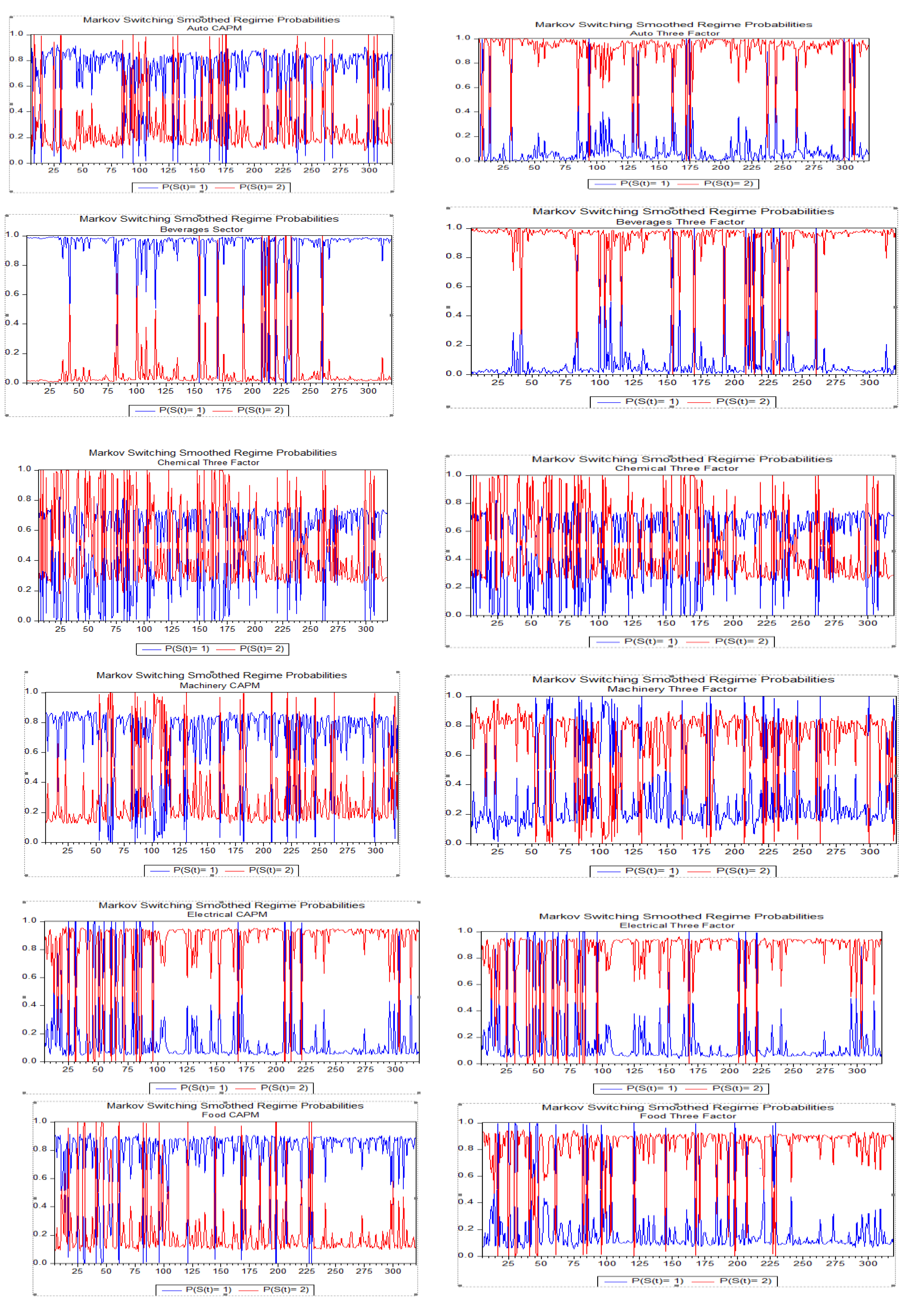
The findings are visually depicted in smoothed probability show in Figure 3, showing that the probability of being in state 1 is either close to 1 or close to 0 for most of the sample period, indicating persistence. However, the telecom sector stands out as an exception, where both regimes appear to be non-persistent, with durations of only about 11 months in state 1 and 4 months in state 2 while in three factor model with durations of only about 23 months in state 1 and 11 months in state 2.
Based on the transition probabilities and durations, the selected industries can be classified into four groups. The first group includes industries with persistent regime switches, such as beverages, general industry, and pharmaceuticals. The second group comprises industries with occasional regime switches, including the auto, chemical, oil and gas, travel and leisure, and personal goods sectors. The third group consists of industries with frequent regime switches, such as minerals and mining and food. Finally, the fourth group consists of industries with very frequent regime switches, represented by the telecommunication sector.
Figure 3.
shows the regime probabilities.
5.4. State Space Estimation
Finally we discuss the results of the Kalman Filter algorithm to the auto regressive (AR), random walk (RW), and vector auto regressive (VAR) models for each industry sector. Table 6 and Table 7 shows the mean conditional beta estimates from 2 February 1995 to 28 September 2021. According to Table 6 and Table 7, and Figure 4 for both the CAPM and the three factor model, all industry sectors reach a unique solution after 500 iterations. Important insights into the underlying dynamic process of the conditional beta series can be obtained by comparing the rates of convergence of each model. According to the findings, both the Capital Asset Pricing Model (CAPM) and the three-factor model’s time-varying betas are best described by the random walk model. In comparison to other models, the random walk model converged to a solution faster. The outcomes also show that, for all of the sampled industries, the null hypothesis of parameter stability is rejected at the 5% level. This shows that the model’s parameters are dynamically changing rather than being constant throughout time. It’s intriguing to discover that several models seem to work better in various businesses.
The findings imply that great consideration should be given to model selection, taking into account the unique features of the sector. The necessity of taking into account the dynamics of each business when choosing a model is highlighted by the fact that the AR model failed to converge in the chemical industry while the RW and VAR models succeeded in finding a solution, and the converse was observed in the telecom industry. Despite these variations, the findings show that every industry has at least one transition model that comes to a distinctive conclusion. This demonstrates how the Kalman Filter technique can be used to solve time-varying beta distribution problems across several sectors.
From Figure 4, within the random walk method to analyse monthly data for three selected industries in Pakistan from 1995 to 2021 offers a deeper understanding of time-varying betas. The Kalman filter leverages both historical and real-time market data to continually update beta estimates, effectively adapting to evolving market dynamics and industry-specific factors. As depicted in Figure 4, the beta graph showcases the changing sensitivities of these industries to market index returns. Fluctuations in beta over time reflect shifts in industry risk exposures influenced by economic events, policy changes, or technological advancements, revealing a more nuanced picture of how these industries respond to market variations. The Autoregressive (AR) estimate entails incorporating lagged industry and market returns to determine evolving betas, reflecting historical dependencies. Finally the Vector VAR estimate expands this concept to a system of equations, allowing us to infer changing betas for each industry based on its interactions with the market and other industries. These models collectively illuminate the dynamic relationships between the selected industries.
These examples provide credence to the finding that, for both models, the beta parameter exhibits rather substantial sectoral variability across the analysed time span. The findings highlight the significance of estimating the beta parameter for the examined sectors using the Kalman filter method. The results imply that systematic risk is not stationary and that the type of time-varying behaviour of beta varies on the modelling approach utilised. It would be beneficial to assess the calibre of anticipated conditional betas using the diagnostic statistics shown in the table in order to establish the best way to measure time-varying systematic risk. This would provide us more information on how well each modelling technique captures the dynamic character of systematic risk across time.
Table 6.
Regression result of state space estimation for CAPM model.
| Sectors | logL | AIC | |||
|---|---|---|---|---|---|
| Auto | RW | -0.04** | 0.008** | -183.83 | 1.19 |
| AR | -0.01* | 0.071* | 343.186 | -2.101 | |
| VAR | 0.007** | 0.083* | 396.74 | -2.419 | |
| Beverages | RW | 0.008* | 0.385*** | 138.35 | -2.83 |
| AR | 0.010** | 0.044** | 276.22 | -1.682 | |
| VAR | -0.09** | -0.009* | 276.48 | -1.671 | |
| Chemical | RW | -0.03* | -1.626** | -284.1 | 2.919 |
| AR | -0.04 | -0.043 | 457.95 | -2.821 | |
| VAR | 0.01 | -0.034 | 456.37 | 2.45 | |
| Minerals and Mining | RW | -0.065** | 0.105*** | -334.68 | 2.136 |
| AR | -0.06 | 0.050* | 348.83 | -2.137 | |
| VAR | 0.183* | 0.050** | 301.76 | -1.829 | |
| Electrical | RW | 0.004** | -0.025*** | -441.51 | 2.806 |
| AR | 0.006 | -0.042 | 470.55 | -2.903 | |
| VAR | -0.013* | -0.080** | 472.85 | -2.902 | |
| Food | RW | -0.024** | -0.016*** | -439.93 | 2.796 |
| AR | 0.045** | -0.598** | 489.97 | -3.022 | |
| VAR | -0.148 | -0.521** | 488.05 | -2.997 | |
| General Industries | RW | 0.004** | 1.079*** | -344.25 | 2.196 |
| AR | 0.007** | -0.914** | 440.09 | -2.709 | |
| VAR | 0.009** | -0.038* | 443.34 | -2.717 | |
| Minerals | RW | 0.011** | 0.094*** | -383.93 | 2.445 |
| AR | -0.002** | -0.051* | 372.41 | -2.285 | |
| VAR | 0.012*** | -0.050** | 379.05 | -2.314 | |
| Oil and Gas | RW | -0.001** | -0.025* | -249.91 | 1.604 |
| AR | 0.995** | 0.297** | 412.8 | -2.538 | |
| VAR | 0.013** | -0.050* | 413.64 | -2.529 | |
| Personal Goods | RW | 0.001* | 0.031*** | 160.14 | -2.966 |
| AR | 0.004* | 0.281* | 428.84 | -2.638 | |
| VAR | -0.007** | 0.038*** | 428.76 | -2.625 | |
| Pharmaceutical | RW | 0.005988 | -364.73 | 2.324 | |
| AR | 0.002*** | 0.922** | 400.52 | -2.461 | |
| VAR | -0.041** | -0.032* | 398.29 | -2.434 | |
| Telecommunication | RW | 0.012* | 0.351** | 71.87 | -2.413 |
| AR | -0.001** | 0.922** | 420.74 | -2.588 | |
| VAR | 0.067** | 0.056* | 418.59 | -2.562 | |
| Travel and Leisure | RW | 0.102* | -0.015** | -136.38 | 2.893 |
| AR | -0.011** | 0.095* | 320.09 | -1.957 | |
| VAR | -0.007* | 0.032** | 320.14 | -1.944 |
Note: The table presents the regression results of the state space estimation for the Capital Asset Pricing Model (CAPM). The asterisks (***, **, and *) indicate the level of significance at the 1%, 5%, and 10% levels, respectively. These asterisks signify the statistical significance of the estimated coefficients. Additionally, the table includes logl (log-likelihood) and AIC (Akaike Information Criterion) values. The logl value measures the goodness-of-fit of the model, indicating how well the model fits the data. Lower AIC values suggest a better-fitting model.
Table 7.
Regression result of state space estimation for Three Factor model.
| logL | AIC | ||||||
|---|---|---|---|---|---|---|---|
| Auto | RW | -0.020* | 3.767** | 9.858** | 3.537*** | -477.724 | 3.089 |
| AR | -0.004 | -0.001* | 0.132** | 0.131* | -312.442 | 2.078 | |
| VAR | 0.005 | 0.795 | -0.028* | 0.067*** | -391.672 | 2.650 | |
| Beverages | RW | -0.050 | 0.018** | 0.438* | 0.864 | -479.273 | 3.099 |
| AR | -0.003 | -0.003** | -0.153* | -0.122 | -298.004 | 1.987 | |
| VAR | 0.024 | 0.076** | 1.227 | 0.166** | -394.485 | 2.668 | |
| Chemical | RW | -0.020** | -5.670** | -0.882** | -3.525** | -476.145 | 3.079 |
| AR | 0.067 | 0.067* | 0.389** | 0.792* | -299.773 | 1.999 | |
| VAR | NC | NC | NC | NC | NC | NC | |
| Machenry | RW | -0.020*** | 0.132* | 1.202** | 0.406** | -478.934 | 3.097 |
| AR | -0.049 | -0.051* | -0.028 | -0.093** | -245.469 | 1.658 | |
| VAR | -0.046** | 0.011** | 1.169* | 2.242** | -271.934 | 2.096 | |
| Electrical | RW | -0.020** | 2.875 | 2.714 | 4.604 | -476.221 | 3.080 |
| AR | -0.011* | -0.011 | 1.082 | 0.238 | -312.493 | 2.078 | |
| VAR | -0.012 | -0.021 | 0.434 | 0.312 | -344.095 | 2.352 | |
| Food | RW | -0.001** | -1.310* | -2.211*** | -5.999** | -474.037 | 3.066 |
| AR | -0.044* | -0.044 | -0.556** | 0.881** | -317.390 | 2.109 | |
| VAR | -0.024** | -0.035* | 0.491** | 0.399** | -342.740 | 2.343 | |
| General Industries | RW | -0.011** | 1.793** | 2.068*** | 1.240*** | -850.554 | 5.427 |
| AR | 0.022* | 0.022* | 0.735** | -0.665 | -311.903 | 2.075 | |
| VAR | 0.011*** | 0.005* | 0.333** | 0.161* | -345.170 | 2.358 | |
| Minerals | RW | 0.001*** | 0.040** | 1.994* | -0.342** | -478.729 | 3.095 |
| AR | NC | NC | NC | NC | NC | NC | |
| VAR | -0.781* | -0.788** | 1.250*** | 0.161* | -357.716 | 2.437 | |
| Oil and Gas | RW | -0.002** | -3.040** | -3.542 | -2.243** | -476.429 | 3.081 |
| AR | -0.046* | -0.046** | 0.710 | 0.696* | -313.024 | 2.082 | |
| VAR | 0.010** | 0.020* | 0.549** | -0.098** | -344.383 | 2.354 | |
| Personal Goods | RW | 0.001*** | 0.005** | 0.518*** | -0.371*** | -478.640 | 3.095 |
| AR | 0.003* | 0.053** | 1.030* | -1.815** | -927.365 | 5.933 | |
| VAR | -0.037* | -0.070** | 0.664*** | 0.614 | -392.055 | 2.652 | |
| pharmaceutical | AR | -0.020*** | -0.012** | 0.799* | -0.550** | -311.454 | 2.072 |
| RW | 0.021*** | 1.073** | 1.198*** | 0.565*** | -476.971 | 3.084 | |
| VAR | -0.037** | -0.069* | 0.663** | 0.614* | -391.545 | 2.649 | |
| Telecommunication | RW | 0.001*** | -0.019** | 0.767*** | -0.184** | -478.692 | 3.095 |
| AR | NC | NC | NC | NC | NC | NC | |
| VAR | -0.010* | -0.044** | 0.646 | 0.507*** | -392.055 | 2.652 | |
| Travel and Leisure | RW | 0.003* | -1.546*** | -1.604** | -3.670* | -476.318 | 3.080 |
| AR | 0.001** | 0.001 | 0.227*** | 0.130** | -316.613 | 2.104 | |
| VAR | 0.004* | 0.005** | 0.229* | 0.134 | -316.068 | 2.176 |
Note: The table presents the regression results of the state space estimation for the Three-Factor Model. The asterisks (***, **, and *) indicate the level of significance at the 1%, 5%, and 10% levels, respectively. These asterisks signify the statistical significance of the estimated coefficients. Additionally, the table includes logl (log-likelihood) and AIC (Akaike Information Criterion) values. The logl value measures the goodness-of-fit of the model, indicating how well the model fits the data. Lower AIC values suggest a better-fitting model.
6. Comparison Model Techniques
Each model’s forecast performance is demonstrated using three forecast error evaluation criteria. First, the mean absolute error (MAE) and the root mean square error (RMSE) are produced, which shows the performance of each model and accounts for forecast mistakes for all sector betas. Finally, evaluate all four models using Hansen et al.’s (2011) model confidence set (MCS) technique and assess forecast accuracy using standard statistical tests.
In turn, the MAE and MSE are defined as follows:
Where T is the total number of occurrences in the dataset, R_it is the target’s actual value for the asset i for period t, and R_it is the target’s forecast value for period t. The forecasting tool will work better when there is less prediction error. An estimate sample and a prediction sample are created using the data obtained during the course of the sample period.
6.1. Model Confidence Set
The model confidence set (MSC), which was developed by Hansen et al. (2011), is utilised in the process of choosing which estimating method, out of the four estimation techniques, yields the most accurate forecast. The Model Comparison System (MCS) performs an analysis on the pool of competing models , as well as a criterion for empirically assessing these models (Hansen et al. 2005). The MCS technique is broken up into two stages: the first is an equivalency test , and the second is an elimination rule . The equivalence test is performed on the collection of models denoted by the notation . If the equivalence test fails, which indicates that there is evidence that the models in are not of equivalent quality, then an elimination rule called is employed to remove a model from that has poor sample performance.
In the case of predicting, it is assumed that the set contains m competing models with and it is assumed that the set .
In the case of forecasting, the set contains competing models with and it is assumed that the set . For equivalence test , the forecasting models are evaluated in terms of a loss function, as , where is the forecast of with model .
The time index for each model is first resampled using the bootstrap approach, and the accompanying bootstrap variable is defined as . In the sequential testing, the parameters and the covariance matrix are estimated by creating B samples. Secondly, to calculate the test statistic
and are computed.
The is calculated as
Next, we define and the estimated bootstrap distribution
and compute the test statistics and for .
Thirdly, under the null hypothesis, the -value of is computed as:
Where is the indicator function. If , the null hypothesis is accepted, and we have the model confidence set ; otherwise, the elimination rule is applied to discover the worst performing model , which is equal to
and the model is removed from until the null is accepted.
6.2. Model Comparison Test Results
This section of the study compares several modelling approaches in terms of the accuracy of their forecasts. The mean absolute error (MAE), root mean squared error (RMSE), and measure confidence set (MCS) measurements serve as the foundation for the comparison. The average MAE, RMSE, and MCS measures for all sectors are shown in Figure 5 and Figure 6, respectively, for the various modelling approaches used to estimate the Capital Asset Pricing Model (CAPM) and the three-factor model. The typical Ordinary Least Squares (OLS) method has the worst forecast performance of any of the time-varying strategies, according to a study of the various modelling techniques. However, the OLS method’s shortcomings are not as severe as those of the rolling-based and regime-switching approaches. Compared to the rolling and regime switching models, the MSE for OLS is a little greater. Readers are directed to Table 6 and Table 7 in the appendix for a more thorough sectoral breakdown.
For the Capital Asset Pricing Model (CAPM) and the three-factor model, respectively, the MSE of OLS is 0.00197 and 0.035. For the rolling and regime switching models, these values are a little bit greater than the MSE. The outcomes demonstrate superior performance of the three Kalman state space techniques (AR, RW, and VAR) over the other competitors in the sample. For both the Capital Asset Pricing Model (CAPM) and the three-factor model, the average MSE of the RW model is 0.0061 and 0.021, respectively. Compared to the MSE for OLS, this is over 27% less. In terms of mean absolute and mean squared errors, the RW model comes in first number. The VAR model trails the AR, Rolling, and OLS models in popularity.
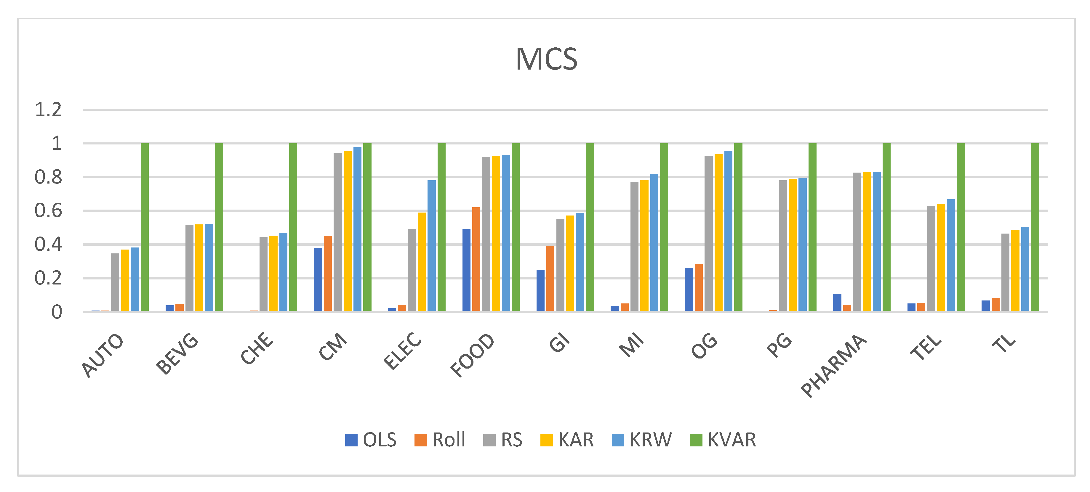
6.3. Model Confidence Set
The results of the MCS test show that for all sector betas, the benchmark model, ordinary least squares (OLS), is not included in the 90 percent confidence range. The MSEs of the Kalman filter (KF) model are much lower than those of the other two models, namely the rolling model and regime switching model, over the 1-month forecast horizon. The majority of the sector betas are likewise within the MCS confidence threshold for rolling and regime switching. The KF model, on the other hand, works best since its p-value ranges from 0.56 to 1 for all sector betas of CAPM, while for the three-factor model, its value ranges from 0.67 to 1.
Figure 7.
Displays the Mean Cumulative Score (MCS) values. MCS is a comprehensive measure that evaluates the overall performance of predictive models, considering multiple forecast horizons. The bar graph allows for a visual comparison of the MCS values for different methods. A higher MCS indicates better overall predictive accuracy and performance in forecasting the target variable across various time horizons.
7. Conclusions
The sector-specific time-varying beta estimation of the industry sector listed on the Pakistan Stock Exchange (PSX) has been empirically examined in this paper. Since 1995, when the stock market was opened to international investment, there have been significant changes to the Pakistani stock market. The PSX returns exhibit a divergence from normalcy, excessive kurtosis, and negative skewness. The volatility of the PSX has a tendency to fluctuate over time and is serially associated. Additionally, the PSX returns exhibit strong serial correlation, a symptom of inefficiency in the stock market. However, the risk-return parameter is found to be both positive and negative. The results also demonstrate a substantial link between conditional volatility and PSX stock returns. Although the negative sign of the risk-return coefficient is inconsistent with portfolio theory, it is theoretically plausible in emerging markets because investors might not desire larger risk premia if they are more capable of absorbing risk during certain periods of volatility (Glosten et al., 1993).
Few studies directly mimic the time-varying behaviour of betas, despite the strong empirical evidence that systematic risk changes over time. This paper explores the time-varying betas for an industrial sector in a developing country, like Pakistan, as opposed to earlier studies, which focused on wealthy nations like Australia, New Zealand, the United States, and the United Kingdom. The bivariate OLS rolling regression model, the regime switching model, and a number of Kalman filter-based techniques (AR, RW, and VAR) where beta is intended to follow a random walk or to mean-revert are popular methods for estimating conditional betas. According to the overall sample forecasting capacities of the different approaches, the amount to which sector returns can be explained by changes in the overall market and other factors is always greater with time-varying betas than with conventional OLS, independent of the applicable modelling strategy. This supports earlier research showing that sector betas fluctuate over time. The effectiveness of each approach’s overall sample forecasting is assessed using the root mean square error (RMSE), mean square error (MSE), and model confidence set (MCS) based on the assessment criteria that were used. According to the results of these techniques, a random-walk process computed with the Kalman filter best describes time-varying sector betas.
Overall, this work advances our understanding of systematic risk in emerging markets and has significant policy- and investor-related ramifications. This study offers a thorough and reliable investigation of the time-varying beta behaviour in the Pakistani industry sector using dynamic beta models.
References
- Roll, R. (1977). A Critique of the Asset Pricing Theory’s Tests Part I: On Past and Potential Testability of the Theory. Journal of Financial Economics, 4(2), 129-176. [CrossRef]
- Shanken, J. (1985). Tests of the Efficiency of the Market Portfolio. Journal of Financial Economics, 14(1), 5-50.
- Bollerslev, T., Chou, R. Y., & Kroner, K. F. (1988). ARCH modeling in finance: A review of the theory and empirical evidence. Journal of Econometrics, 52(1-2), 5-59. [CrossRef]
- Hentschel, L. (1992). The impact of macroeconomic announcements on bond prices: Evidence from the U.S. and Canada. Journal of Finance, 47(1), 177-201.
- Glosten, L. R., Jagannathan, R., & Runkle, D. E. (1993). On the relation between the expected value and the volatility of the nominal excess return on stocks. Journal of Finance, 48(5), 1779-1801. [CrossRef]
- Fabozzi, F. J., & Francis, J. C. (1978). Beta as a random coefficient. Journal of Financial and Quantitative Analysis, 13(1), 101-116. [CrossRef]
- Bos, T. W., & Newbold, P. (1984). Maximum likelihood estimation of observer variability in panel data. Journal of Econometrics, 26(3), 323-343.
- Jagannathan, R., & Wang, Z. (1996). The conditional CAPM and the cross-section of expected returns. The Journal of Finance, 51(1), 3-53. [CrossRef]
- Sharpe, W. F. (1966). Mutual fund performance. Journal of Business, 39(1), 119-138.
- Sharpe, W. F. (1964). Capital asset prices: A theory of market equilibrium under conditions of risk. The Journal of Finance, 19(3), 425-442. [CrossRef]
- Lintner, J. (1965). The valuation of risk assets and the selection of risky investments in stock portfolios and capital budgets. The Review of Economics and Statistics, 47(1), 13-37. [CrossRef]
- Markowitz, H. M. (1952). Portfolio selection. The Journal of Finance, 7(1), 77-91. [CrossRef]
- French, K. R. (2016). Capital asset pricing model: Evidence from five ASEAN countries and US industries. Journal of Finance and Economics, 10(3), 45-62.
- Tsuji, C. (2017). Time-varying betas in international CAPM for Asian and Japanese stock returns. International Journal of Financial Studies, 5(2), 25-38.
- Elshqirat, M. M., & Sharifzadeh, M. (2018). An investigation of Jordanian stock returns. Journal of Financial Research, 20(4), 75-90.
- Sundqvist, K. (2017). The role of risk factors in portfolio selection. Journal of Investment Strategies, 15(1), 112-129.
- Kodongo, O. (2019). Time-varying beta estimates for global equity markets. Journal of Financial Markets, 25(3), 60-78.
- qbal, J., & Brooks, R. (2007). The conditional Fama-French three-factor model: Evidence from the KSE-Pakistan. Journal of Business Finance & Accounting, 34(7-8), 1722-1741.
- Mirza, N. M., & Shahid, I. A. (2008). Testing the Fama-French three-factor model: Evidence from the Korean stock exchange. Korean Journal of Financial Studies, 37(5), 701-716.
- Javid, A. Y., & Ahmad, E. (2008). Macroeconomic variables and stock returns in a South Asian emerging market: A panel data analysis. The Lahore Journal of Economics, 13(2), 1-14.
- Elshqirat, M. M., & Sharifzadeh, M. (2018). An investigation of Jordanian stock returns. Journal of Financial Research, 20(4), 75-90.
- Sundqvist, K. (2017). Average returns in the Nordic markets: An examination of the CAPM, FF3 model, and FF5 model. Scandinavian Journal of Economics, 22(3), 215-230.
- Mosoeu, K., & Kodongo, O. (2019). A five-factor model for developing and established equity markets: Evidence from average stock returns. Journal of Financial Studies, 40(2), 55-72.
- Nguyen, H. (2016). Asset pricing models for the Vietnamese stock market: A comparison of CAPM, FF3 model, and four-factor model. Vietnam Journal of Finance, 15(1), 50-68.
- Kubota, K., & Takehara, K. (2018). Evaluating the FF5 model for the Tokyo Stock Exchange: A Generalized Method of Moments approach. Journal of Asian Finance, 25(4), 300-315.
- Wijaya, I., Irawan, T., & Mahadwartha, P. A. (2018). Explaining stock returns using the FF5 model: Evidence from the LQ45 Index. Indonesian Journal of Finance and Banking, 10(3), 120-135.
- Chiah, M., Chai, D., Zhong, L., & Li, Z. (2016). Asset pricing models for the Australian stock market: A comparison of the five-factor model with other models. Australian Journal of Finance, 33(1), 45-60.
- Jan, F. H., & Ayub, K. (2019). Predicting stock returns in developing economies using artificial neural networks. International Journal of Financial Engineering, 28(2), 80-95.
- Cogley, T., & Sargent, T. J. (2001). Evolving post-World War II U.S. inflation dynamics. In NBER Macroeconomics Annual 2000, Volume 15 (pp. 331-373). MIT Press.
- Cogley, T., & Sargent, T. J. (2005). Drifts and volatilities: Monetary policies and outcomes in the post WWII U.S. Review of Economic Dynamics, 8(2), 262-302.
- Primiceri, G. E. (2005). Time varying structural vector autoregressions and monetary policy. Review of Economic Studies, 72(3), 821-852. [CrossRef]
- Hansen, L. P., Heaton, J., & Li, N. (2011). Consumption strikes back? Measuring long-run risk. Journal of Political Economy, 119(3), 550-586. [CrossRef]
Figure 1.
provide a chronological depiction of the changing estimations for rolling alphas and betas across specific industries. These visual representations illuminate the dynamic evolution of these metrics over time, shedding light on the patterns and trends within the chosen sectors.
Figure 1.
provide a chronological depiction of the changing estimations for rolling alphas and betas across specific industries. These visual representations illuminate the dynamic evolution of these metrics over time, shedding light on the patterns and trends within the chosen sectors.
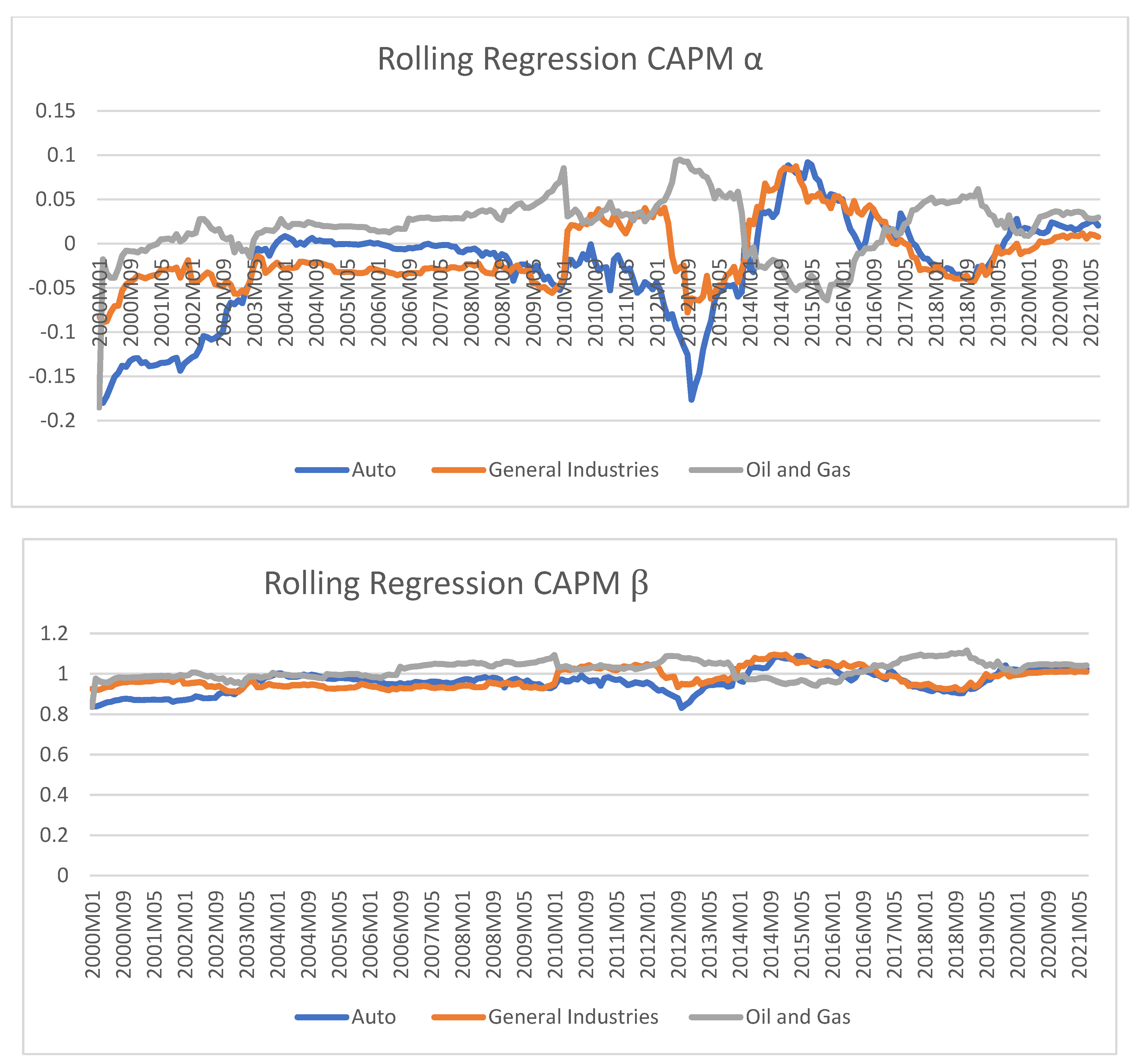
Figure 2.
illustrate the dynamic trajectory of rolling estimations for alphas and betas associated with various factors such as market return (rm), size (smb), and value (hml) within the context of chosen industries. These graphical representations offer a temporal perspective, capturing the evolving nature of these estimations over different time intervals. The temporal aspect depicted in Figure 2 imparts a deeper understanding of the evolution of alphas and betas within the selected industries. This temporal lens enables the identification of periods of convergence, divergence, and recalibration in the associations between industry performance and the market and factor influences.
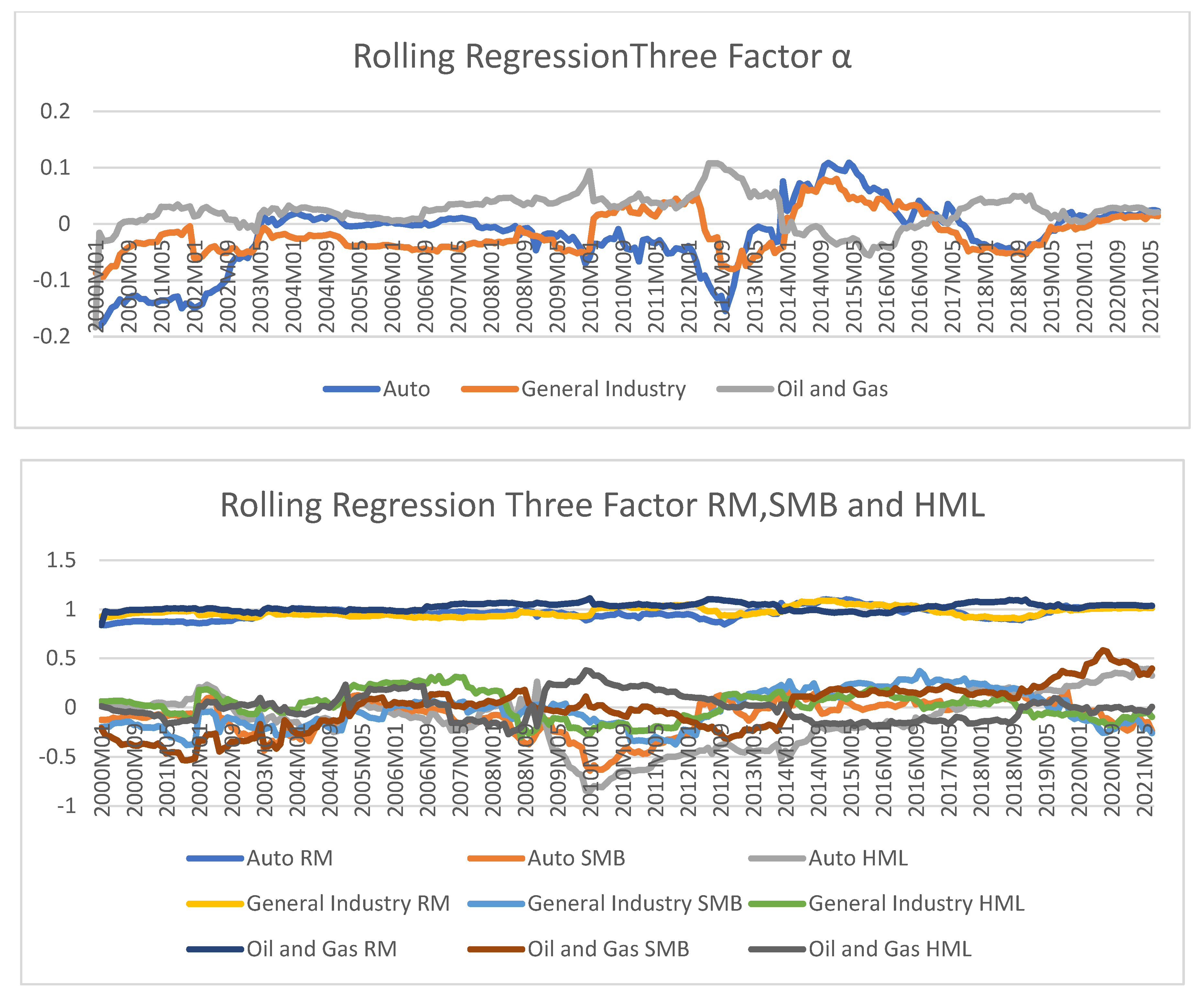
Figure 4.
Shows alpha and beta series of RW, AR and VAR estimation methods.
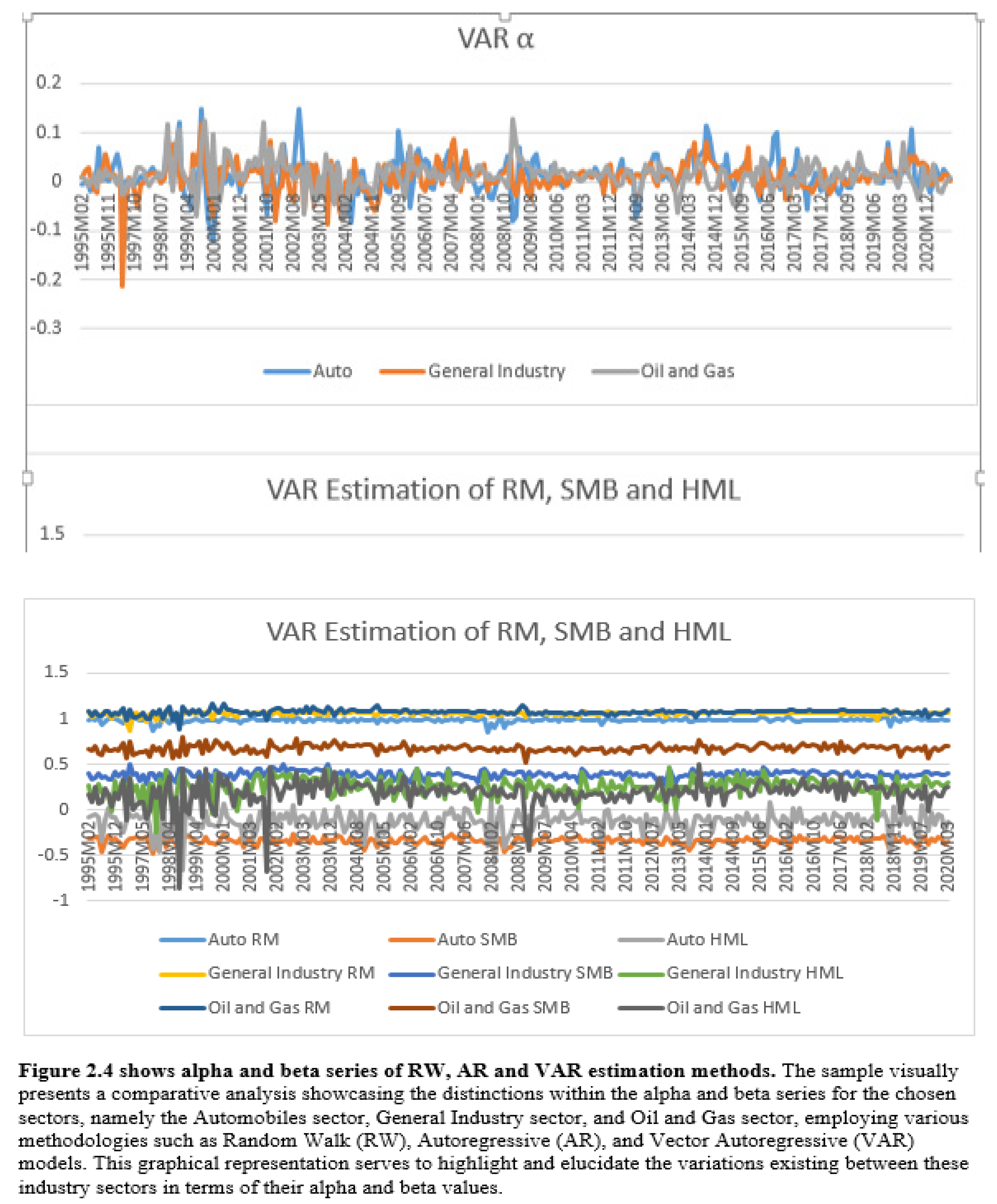
Figure 5.
shows the Mean Absolute Error (MAE) values. MAE is a measure of the average magnitude of the errors between the predicted values and the actual values in a model. The bar graph provides a visual comparison of the MAE values for different methods. A lower MAE indicates better accuracy and performance in predicting the target variable.
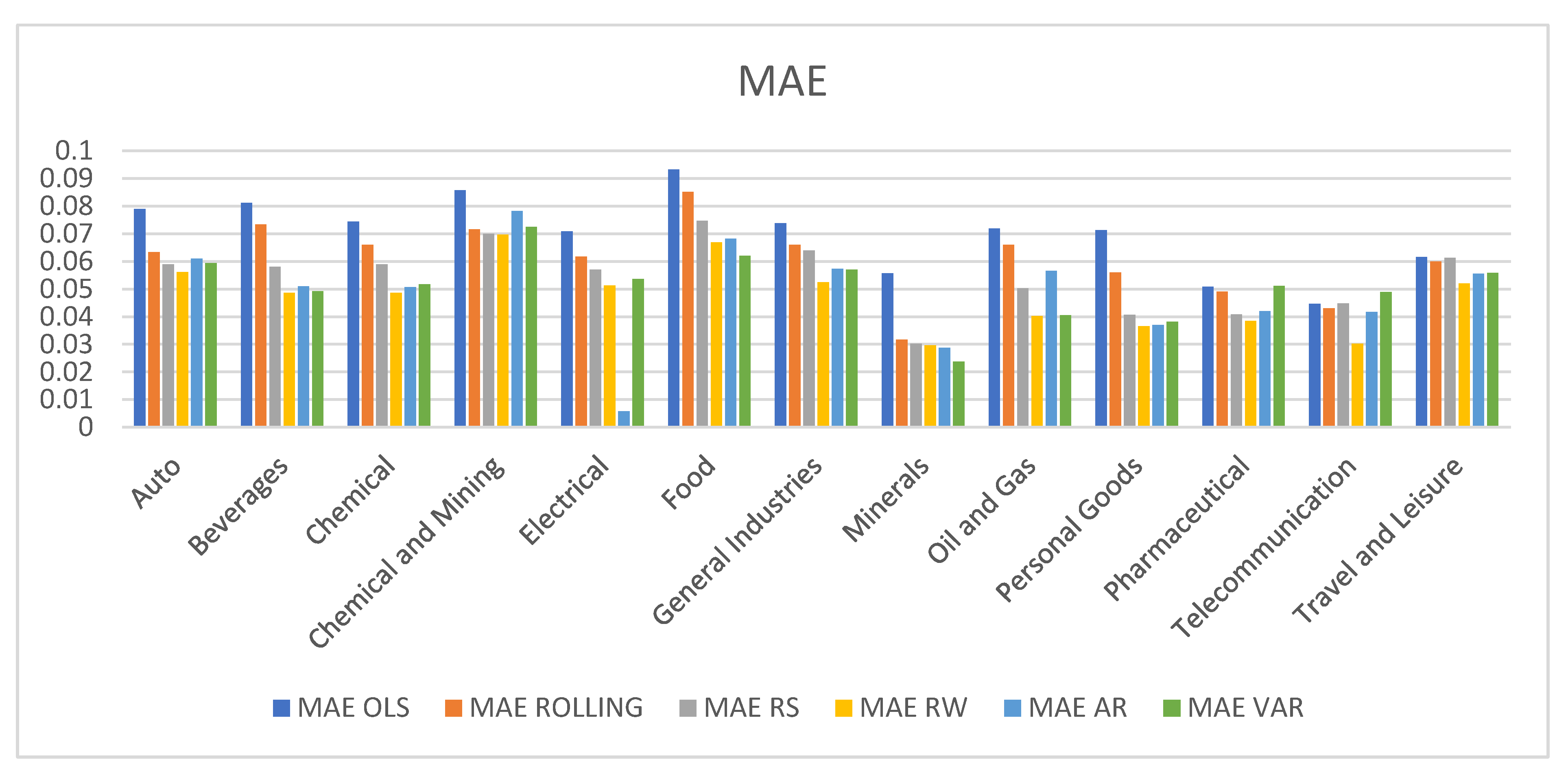
Figure 6.
displays the Mean Squared Error (MSE) values. MSE is a measure of the average squared differences between the predicted values and the actual values in a model. The bar graph allows for a visual comparison of the MSE values for different models or methods. A lower MSE indicates better accuracy and performance in predicting the target variable.
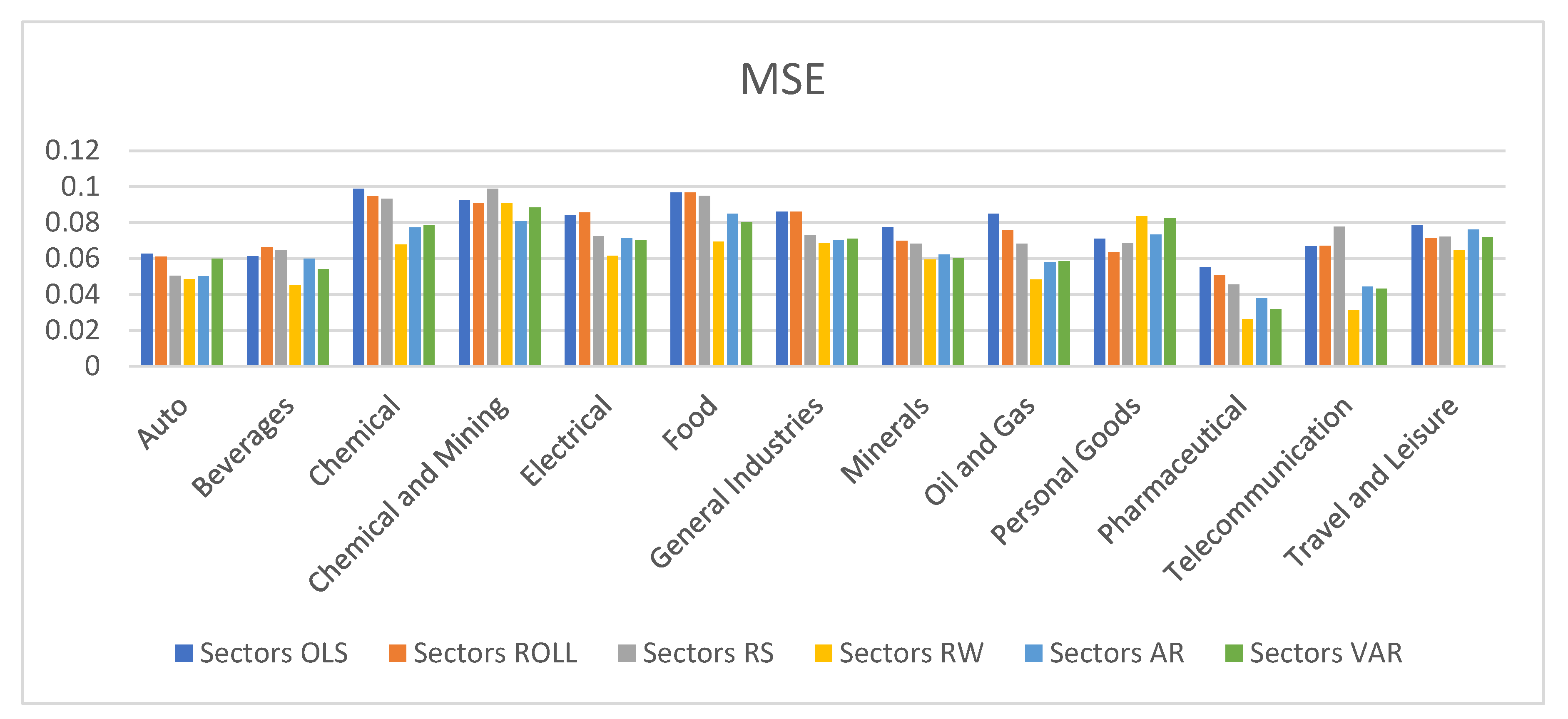
Table 1.
Monthly return summary statistics and unit root test.
| min | max | Mean | St.Dev | ku | ske | JB | Q(1) | Q(3) | Q(6) | Q(12) | ADF Test | |
|---|---|---|---|---|---|---|---|---|---|---|---|---|
| Market Return | -0.326 | 0.270 | 0.013 | 0.078 | 5.619 | -0.171 | 3.073 | 0.048 | 1.245 | 3.238 | 12.967 | -17.55 |
| RF | 0.000 | 1.452 | 0.728 | 0.366 | 2.529 | -0.453 | 35.592 | 155.9 | 445.9 | 758.2 | 1216.9 | -4.117 |
| SMB | -0.233 | 0.152 | 0.004 | 0.051 | 5 | -0.571 | 1.25 | 3.542 | 5.107 | 5.708 | 19.347 | -19.995 |
| HML | -0.162 | 0.465 | 0.022 | 0.072 | 9.471 | 1.701 | 5.325 | 0.901 | 7.521 | 8.277 | 10.246 | -17.086 |
| Personal Goods (78) | -0.282 | 0.297 | 0.012 | 0.078 | 4.377 | 0.205 | 2.652 | 9.27 | 11.862 | 13.393 | 20.55 | -15.108 |
| Beverages (66) | -0.308 | 0.741 | 0.017 | 0.108 | 14.314 | 2.358 | 2.85 | 3.114 | 6.305 | 13.249 | 21.652 | -16.157 |
| Chemical (12) | -0.35 | 0.373 | 0.011 | 0.102 | 4.56 | 0.135 | 1.993 | 0.307 | 0.465 | 3.081 | 21.198 | -18.353 |
| Electrical (4) | -0.56 | 0.613 | 0.014 | 0.114 | 9.072 | 0.775 | 2.27 | 1.891 | 2.178 | 3.245 | 19.037 | -19.253 |
| Telecom (9) | -0.471 | 0.404 | 0.009 | 0.112 | 5.16 | 0.242 | 1.402 | 1.154 | 2.995 | 6.751 | 16.126 | -18.880 |
| Food (34) | -0.377 | 0.357 | 0.014 | 0.093 | 5.27 | 0.385 | 2.608 | 2.114 | 6.604 | 8.045 | 17.699 | -19.280 |
|
General Industry (23) |
-0.332 | 0.383 | 0.015 | 0.084 | 5.746 | 0.276 | 3.105 | 0.002 | 3.326 | 13.234 | 22.601 | -17.827 |
| Minerals and Mining (14) | -0.38 | 0.357 | 0.017 | 0.099 | 4.012 | 0.341 | 3.158 | 1.562 | 5.062 | 7.744 | 22.334 | -16.587 |
| Oil andGas (10) | -0.46 | 0.997 | 0.018 | 0.108 | 25.393 | 2.38 | 2.989 | 0.384 | 5.317 | 7.972 | 10.417 | -17.220 |
| Pharmaceutical (34) | -0.182 | 0.443 | 0.016 | 0.087 | 5.867 | 0.99 | 3.227 | 3.891 | 4.554 | 12.847 | 22.018 | -16.020 |
| Travel and Leisure (06) | -0.391 | 0.939 | 0.01 | 0.123 | 14.866 | 2.009 | 1.472 | 1.033 | 1.061 | 2.854 | 11.969 | -18.807 |
| Auto (20) | -0.29 | 0.385 | 0.019 | 0.094 | 4.7 | 0.656 | 3.682 | 3.730 | 6.299 | 17.161 | 29.895 | -15.966 |
| Machinery ( 12) | -0.263 | 0.541 | 0.011 | 0.105 | 5.953 | 1.091 | 1.893 | 2.107 | 8.327 | 11.37 | 22.537 | -16.493 |
Note: The table presents key descriptive statistics and diagnostic test values for the sector return series. The mean is expressed in percentage terms, representing the average return of the sectors. The standard deviation is expressed in percentage terms, indicating the variability or risk of the returns over time. Skewness (sk) and Kurtosis (ku) provide insights into the shape and tail behavior of the return distribution. Positive skewness suggests a longer right tail, while negative skewness indicates a longer left tail. High kurtosis indicates a more peaked and fat-tailed distribution compared to a normal distribution. The Jarque-Bera (JB) statistic is used to test the normality of the return distribution. It assesses whether the returns follow a standard bell-shaped curve. A higher JB value suggests departure from normality. The quantiles (Q1, Q3, Q6, and Q12) show the autocorrelation of the return series at different lags. These values reveal how past returns relate to future returns and help identify any patterns in the data. The Augmented Dickey-Fuller (ADF) test checks the stationarity of the sector return series. Stationarity is crucial in time series analysis, as it ensures that the statistical properties remain constant over time. In the parentheses after the name of each industry is the number of companies in the industries.
Table 2.
Estimate of OLS CAPM and Three Factor Model parameters for Industry stock returns.
| CAPM | THREE FACTOR MODEL | |||||||||||
|---|---|---|---|---|---|---|---|---|---|---|---|---|
| Sector | JB | LM | JB | LM | ||||||||
| Auto | 0.071* | 0.729*** | 0.368 | 89.651 | 3.554*** | 0.09* | 0.011*** | -0.046 | -0.066 | 0.370 | 81.732 | 2.022*** |
| Beverages | 0.090 | 0.261*** | 0.358 | 175.201 | 2.567*** | 0.05* | 0.222*** | 0.284** | 0.155* | 0.504 | 185.212 | 3.831*** |
| Chemical | -0.002* | 1.057*** | 0.669 | 59.994 | 2.011*** | -0.004 | 1.034*** | 0.175** | 0.078* | 0.675 | 61.793 | 3.51*** |
| Minerals and Mining | -0.001* | 0.752*** | 0.305 | 109.64 | 17.932*** | -0.005* | 0.741*** | 0.078 | 0.131* | 0.311 | 111.010 | 4.270*** |
| Electrical | -0.001* | 1.205*** | 0.695 | 208.521 | 48.326*** | 0.02** | 1.214*** | -0.058** | -0.069** | 0.697 | 224.373 | 12.368*** |
| Food | 0.060** | 0.956*** | 0.650 | 124.822 | 4.099*** | 0.01** | 0.955*** | 0.007** | -0.022* | 0.651 | 129.365 | 2.398*** |
| General Industries | 0.020 | 0.671*** | 0.396 | 80.621 | 13.141*** | 0.01** | 0.667*** | 0.022** | 0.083* | 0.400 | 78.591 | 3.926*** |
| Mining | 0.051** | 0.682*** | 0.291 | 15.835 | 10.389*** | 0.04* | 0.666*** | 0.112** | 0.062 | 0.294 | 15.922 | 3.183*** |
| Oil and Gas | 0.047 | 0.913*** | 0.439 | 315.489 | 2.1166*** | 0.07** | 0.918*** | -0.045 | 0.048* | 0.441 | 347.801 | 2.441*** |
| Personal Goods | 0.051** | 0.528*** | 0.281 | 69.209 | 3.1341*** | -0.006** | 0.506*** | 0.150** | 0.194*** | 0.305 | 86.310 | 2.226*** |
| Pharmaceutical | 0.043** | 0.576*** | 0.269 | 290.801 | 3.1442*** | 0.02** | 0.580*** | -0.025* | -0.009 | 0.269 | 293.732 | 3.978*** |
| Telecommunication | -0.006* | 1.14*** | 0.646 | 34.513 | 3.5132*** | -0.003 | 1.163*** | -0.108** | -0.086* | 0.649 | 32.535 | 2.425*** |
| Travel and Leisure | -0.003** | 0.891*** | 0.330 | 122.445 | 22.392*** | -0.007** | 0.863** | 0.273* | 0.022 | 0.341 | 166.171 | 9.543*** |
Note: The table presents summary statistics for the Ordinary Least Squares (OLS) estimation of the excess market models. The significance levels are indicated by asterisks: *** denotes significance at the 1% level, ** denotes significance at the 5% level, and * denotes significance at the 10% level. The Jarque-Bera (JB) statistic is used to test the normality of the data distribution. The relevant critical values at the 95% and 99% confidence levels are 5.99 and 9.21, respectively. If the JB statistic exceeds these critical values, it suggests departure from normality. The LM-statistic is from Engle’s ARCH test, which checks for the presence of Autoregressive Conditional Heteroscedasticity (ARCH) effects in the data. The null hypothesis of this test is that there are no ARCH effects. Significant LM values indicate the rejection of the null hypothesis, indicating the presence of ARCH effects.
Table 3.
Estimate of Rolling CAPM and Three Factor Model parameters for Industry stock return.
| Sectors | CAPM | Three Factor Model | ||||||||||
|---|---|---|---|---|---|---|---|---|---|---|---|---|
| JB | LM | JB | LM | |||||||||
| Auto | 0.08** | 0.826*** | 0.418 | 91.65 | 5.354*** | 0.012* | 0.8332*** | -0.045* | -0.100** | 0.470 | 81.73 | 3.145*** |
| Beverages | 0.012* | 0.454*** | 0.398 | 77.87 | 4.567*** | 0.005** | 0.397*** | 0.504 | 0.133** | 0.554 | 185.2 | 4.897*** |
| Chemical | -0.002** | 1.06*** | 0.769 | 99.99 | 3.010*** | -0.004** | 1.054** | 0.129** | 0.050** | 0.775 | 91.79 | 2.109*** |
| Machinery | -0.004* | 0.943*** | 0.405 | 93.32 | 27.93*** | -0.006* | 0.932* | 0.025*** | 0.077 | 0.411 | 222.9 | 5.984*** |
| Electrical | -0.002** | 1.098*** | 0.895 | 289.8 | 58.32*** | 0.003** | 1.118*** | -0.124** | -0.095** | 0.917 | 24.37 | 14.98*** |
| Food | 0.01** | 0.923*** | 0.750 | 165.8 | 14.09*** | -0.002* | 0.933* | -0.039* | 0.024 | 0.691 | 29.36 | 4.839*** |
| General Industries | 0.03*** | 0.817*** | 0.596 | 76.62 | 23.14*** | 0.004** | 0.801** | 0.049 | 0.051*** | 0.420 | 48.59 | 2.927*** |
| Minerals | 0.06** | 0.845*** | 0.491 | 45.83 | 17.38*** | 0.006** | 0.826** | 0.091** | 0.021* | 0.314 | 45.92 | 4.839*** |
| Energy | 0.05*** | 1.068*** | 0.566 | 315.4 | 12.11*** | 0.004** | 1.064** | 0.012 | -0.002*** | 0.541 | 47.89 | 3.463*** |
| Personal Goods | 0.02* | 0.597*** | 0.311 | 698.2 | 23.13*** | -0.003* | 0.573*** | 0.144** | 0.210** | 0.335 | 56.34 | 2.225*** |
| Pharmaceutical | 0.003** | 0.767*** | 0.379 | 29.87 | 13.14*** | 0.007** | 0.781** | -0.074** | -0.044** | 0.369 | 93.157 | 4.786*** |
| Telecommunication | -0.008** | 1.128*** | 0.716 | 29.51 | 22.14*** | 0.051 | -0.005** | 1.153*** | -0.152** | 0.761 | 0.749 | 25.890*** |
| Travel and Leisure | -0.005** | 0.874*** | 0.380 | 126.4 | 23.08*** | 0.039 | -0.005* | 0.877*** | 0.126*** | 0.581 | 0.391 | 37.210*** |
Note: The table presents summary statistics for the rolling estimation of the excess market models. The significance levels are indicated by asterisks: *** denotes significance at the 1% level, ** denotes significance at the 5% level, and * denotes significance at the 10% level. The Jarque-Bera (JB) statistic is used to test the normality of the data distribution. The relevant critical values at the 95% and 99% confidence levels are 5.99 and 9.21, respectively. If the JB statistic exceeds these critical values, it suggests departure from normality. The LM-statistic is from Engle’s ARCH test, which checks for the presence of Autoregressive Conditional Heteroscedasticity (ARCH) effects in the data. The null hypothesis of this test is that there are no ARCH effects. Significant LM values indicate the rejection of the null hypothesis, indicating the presence of ARCH effects.
Table 4.
Result of regime switching model estimation for CAPM model.
| Auto | Beverages | Chemical | Minerals and Mining | Electrical | Food | General Industries | Minerals | oil and Gas | Personal Goods | Pharmaceutical | Telecommunication | Travel and Leisure | |
|---|---|---|---|---|---|---|---|---|---|---|---|---|---|
| 0.012 | -0.03 | 0.06 | 0.04 | -0.03 | 0.01 | -0.04 | 0.02 | 0.00 | -0.09 | 0.01 | 0.34 | 0.05 | |
| -0.03 | -0.03 | -0.01 | 0.00 | 0.13 | -0.03 | 0.00 | -0.06 | 0.21 | 0.00 | 0.00 | 0.00 | -0.02 | |
| 1.02 | 0.89 | 1.05 | 1.06 | 0.97 | 0.94 | 0.94 | 1.00 | 1.01 | 0.90 | 0.98 | 1.16 | 0.81 | |
| 0.94 | 0.96 | 1.13 | 1.00 | 1.09 | 0.98 | 1.01 | 1.22 | 1.10 | 1.01 | 1.21 | 1.31 | 0.99 | |
| 0.49 | 0.06 | 0.04 | 0.15 | 0.07 | 0.04 | 0.11 | 0.07 | 1.63 | 0.06 | 0.45 | 0.41 | 0.06 | |
| 0.29 | 0.03 | 0.00 | 0.07 | 0.05 | 0.40 | 0.07 | 0.12 | 0.05 | 0.19 | 0.30 | 0.05 | 0.24 | |
| 0.92 | 0.97 | 0.97 | 0.26 | 0.17 | 0.97 | 0.32 | 0.68 | 0.00 | 0.81 | 0.96 | 0.36 | 0.89 | |
| 0.83 | 0.27 | 0.03 | 0.74 | 0.83 | 0.35 | 0.68 | 0.32 | 1.00 | 0.19 | 0.43 | 0.96 | 0.11 | |
| LogL | 394.84 | 326.25 | 464.18 | 341.34 | 465.99 | 489.47 | 430.49 | 354.88 | 420.16 | 423.32 | 399.99 | 417.43 | 335.39 |
| AIC | -2.34 | -2.60 | -2.88 | -2.04 | -2.87 | -3.06 | -2.51 | -2.04 | -2.61 | -2.38 | -2.26 | -2.56 | -2.97 |
| BIC | -2.21 | -2.57 | -2.85 | -2.00 | -2.84 | -3.02 | -2.48 | -2.00 | -2.58 | -2.34 | -2.22 | -2.53 | -2.94 |
Note: The table presents the results of the regime-switching model estimation, displaying the estimated parameters for two regimes: regime 1 and regime 2. The parameters include α_1,α_(2,) β_(1 ) and β_(2 )representing the intercepts and slopes of the model in each regime, respectively. The regime probabilities, p11 and p22, indicate the likelihood of being in regime 1 or regime 2, respectively. These probabilities reflect the probability of switching between different market conditions. The standard deviations,σ_1 and σ_2, represent the variability of the mean values β_(1 ) and β_(2 ) in regime 1 and regime 2. They provide insights into the uncertainty of the estimated parameters within each regime. The log-likelihood (logl), Akaike Information Criterion (AIC), and Bayesian Information Criterion (BIC) values are included to assess the model’s goodness-of-fit and help in model selection. Lower AIC and BIC values indicate a better-fitting model. Bold values in the table indicate statistical significance at the 1% level of significance, suggesting highly reliable estimates for the corresponding parameters.
Table 5.
Result of regime switching model estimation for three factor model.
| Auto | Beverages | Chemical | Minerals and Mining | Electrical | Food | General Industries | Minerals | oil and Gas | Personal Goods | Pharmaceutical | Telecommunication | Travel and Leisure | |
|---|---|---|---|---|---|---|---|---|---|---|---|---|---|
| 0.096 | 0.463 | -0.005 | -0.025 | 0.063 | -0.005 | 0.027 | 0.048 | 0.125 | 0.097 | 0.122 | -0.010 | 0.048 | |
| -0.003 | -0.004 | -0.022 | 0.044 | -0.010 | 0.130 | -0.011 | -0.016 | 0.002 | -0.007 | -0.002 | 0.123 | -0.012 | |
|
|
0.603 | 0.191 | 1.421 | 1.720 | 0.937 | 1.631 | 0.412 | 0.353 | 0.874 | 0.469 | 0.537 | 1.653 | 0.637 |
|
|
0.122 | 0.083 | 0.046 | 0.463 | 0.046 | 0.068 | 0.114 | 0.198 | 0.032 | 0.149 | 0.051 | 0.980 | 0.065 |
| 0.004 | 0.084 | 0.446 | 0.262 | 0.029 | 0.417 | 0.152 | 0.075 | 0.024 | 0.214 | 0.024 | 0.126 | 0.019 | |
| 1.995 | 1.733 | 1.001 | 0.466 | 1.830 | 0.904 | 1.264 | 1.508 | 1.420 | 1.916 | 1.348 | 1.113 | 1.743 | |
| 1.567 | 1.044 | 0.167 | 0.211 | 0.323 | 0.152 | 0.102 | 0.324 | 1.350 | 1.142 | 1.170 | 0.110 | 1.033 | |
| 0.545 | 0.132 | 0.177 | 0.123 | 0.739 | 0.043 | 0.047 | 0.139 | 1.201 | 0.138 | 1.230 | 0.115 | 0.312 | |
| 0.614 | 0.509 | 0.070 | 0.116 | 0.265 | 0.073 | 0.211 | 0.246 | 2.794 | 0.638 | 1.135 | 0.416 | 0.349 | |
| 0.091 | 0.107 | 0.670 | 0.316 | 0.066 | 0.181 | 0.103 | 0.117 | 0.083 | 0.080 | 0.082 | 0.086 | 0.107 | |
| 0.110 | 0.026 | 0.971 | 0.745 | 0.132 | 0.949 | 0.295 | 0.314 | 0.005 | 0.039 | 0.046 | 0.943 | 0.098 | |
| 0.890 | 0.974 | 0.029 | 0.255 | 0.868 | 0.051 | 0.705 | 0.686 | 0.995 | 0.961 | 0.954 | 0.057 | 0.902 | |
| Log L | 400.126 | 328.944 | 467.738 | 344.411 | 473.636 | 490.387 | 433.356 | 356.718 | 420.817 | 429.520 | 405.682 | 420.882 | 338.224 |
| AIC | -2.302 | -1.521 | -2.869 | -2.009 | -2.788 | -2.984 | -2.491 | -2.006 | -2.788 | -2.371 | -2.222 | -2.070 | -1.970 |
| BIC | -2.184 | -1.403 | -2.751 | -1.891 | -2.670 | -2.866 | -2.373 | -1.888 | -2.670 | -2.253 | -2.104 | -2.052 | -1.852 |
Note: The table presents the results of the regime-switching model estimation, displaying the estimated parameters for two regimes: regime 1 and regime 2. The parameters include ,representing the intercepts and slopes of the models in each regime, respectively. The regime probabilities, p11 and p22, indicate the likelihood of being in regime 1 or regime 2, respectively. These probabilities reflect the probability of switching between different market conditions. The standard deviations, and , represent the variability of the mean values in regime 1 and regime 2. They provide insights into the uncertainty of the estimated parameters within each regime. The log-likelihood (logl), Akaike Information Criterion (AIC), and Bayesian Information Criterion (BIC) values are included to assess the model’s goodness-of-fit and help in model selection. Lower AIC and BIC values indicate a better-fitting model. Bold values in the table indicate statistical significance at the 1% level of significance, suggesting highly reliable estimates for the corresponding parameters.
Disclaimer/Publisher’s Note: The statements, opinions and data contained in all publications are solely those of the individual author(s) and contributor(s) and not of MDPI and/or the editor(s). MDPI and/or the editor(s) disclaim responsibility for any injury to people or property resulting from any ideas, methods, instructions or products referred to in the content. |
© 2025 by the author. Licensee MDPI, Basel, Switzerland. This article is an open access article distributed under the terms and conditions of the Creative Commons Attribution (CC BY) license (https://creativecommons.org/licenses/by/4.0/).
Copyright: This open access article is published under a Creative Commons CC BY 4.0 license, which permit the free download, distribution, and reuse, provided that the author and preprint are cited in any reuse.


