Railway Transition Curves Curvature for High-Speed Trains – Should It Be Smooth in the Extreme Points or Not, or Something Else?

1. Introduction

In the contemporary world, we observe a growing passenger flow in both road and railway transport. Over time, more and more countries construct modern road and railway infrastructure. In the field of railway infrastructure, the growing number of railway lines constructed for high-speed trains is observed, mainly in Europe and Asia. Railway infrastructure for such trains needs the proper line geometry. Here, the most essential characteristics are large circular arc radii and a suitable shape (and length) of transition curves (TCs), spanning between a straight track and the circular arc.

The modern railway infrastructure is a witness to new shapes of railway transition curves (TCs). In railway engineering, not only the 3^rd degree parabola (curve characterized by linear change of the curvature in the longitudinal coordinate x function and of the vehicle lateral acceleration, too) is used mainly by engineers-practitioners. Historically, the Bloss curve is a second crucial transition curve. The Bloss curve is, in fact, a polynomial transition curve of the 5^th degree.

The fundamental difference between the above-mentioned two curves is the shape of the curvature. The 3^rd degree parabola has bends at the extreme curve points (beginning and the end point of the curve), so it has the continuity of type G₀. Bloss curve is smooth in the extremities, so this curve has the continuity of G₁ type (a tangency in strictly mathematical reasoning).

2. The Main Aim of the Current Work

The general aim of this work is to answer questions about the desirable features of railway transition curves’ curvature, especially at the extreme points. The cause is the ambiguous results of the TC optimizations obtained by the authors, presented in [1,2]. They are twofold, different for the 5^th and 7^th degrees of polynomial TCs than for the 9^th and 11^th degrees. The obtained optimum curves of 5^th and 7^th degrees possess the bends at curvature extreme points (like for the parabola of the 3^rd degree). The curvatures of optimum TCs of the 9^th and 11^th degrees are close to smooth curves, with slight bends preserved. It happens despite the same quality functions for these cases, TC lengths adopted consequently for them according to engineering formulas (e.g. [3]), and starting TC shapes in the optimization are always adopted with perfectly smooth curvatures (no bends).

The above-mentioned discrepancy of curvatures, dependent on the TC’s degree, results in the main detailed aim of this work. It is to find the main factor that influences the existence of bends at the extreme points of the curvatures of optimum railway TCs. So, the authors mean here the existence of the continuity of the type of G₀ or G₁. For this purpose, a hypothesis that causes such a situation was formulated.

The mentioned hypothesis is as follows:

“The reason is time, more specifically, a large enough amount of time while negotiating the whole curve length. If the railway vehicle needs a long negotiation time, then vehicle dynamics can be smoother.” It is essential, as the present authors use a full dynamical model (as in railway dynamics studies) while calculating the quality functions, instead of the vehicle represented by a single point (as in civil engineering approaches to TCs assessment and design).

A long time of curve negotiation by the vehicle can be achieved in two ways:

-

very long length of the curve and “normal” velocity of the vehicle,

-

small vehicle velocity and “normal” length of the vehicle.

Under the concept of a “normal” length and velocity, the values of these parameters, calculated using the engineering formulas, should be understood here.

In the current work, its authors performed the optimization of railway transition curves, modelled by the polynomials of 5^th, 9^th, and 11^th degrees. For the 9^th and 11^th degrees, TCs’ feature of their great typical length was useful. The optimizations were also supplemented by the simulations of the single passage of the vehicle through a chosen railway curve to demonstrate the railway vehicle dynamics at the extreme points of the curve.

Previously, the authors tried to prove the analogous hypotheses, taking greater account of the influence of the TC’s initial and end zones, the quality function based on jerk in TC, and the higher values of the curve radius R. They turned out to be untrue.

3. Short Literature Survey

Many works relating to railway transition curves are currently published. Mainly, it is visible in the light of the geometry of the construction of new high-speed train lines. The important works relating to railway transition curves are represented, e.g., by Tari and Baykal, Hasslinger, Long et al., and Kufver.

Tari and Baykal, in [4], introduced kinematical parameter - lateral change of acceleration - of railway vehicle during the TC negotiating as the crucial criterion for passenger comfort assessment in this zone. The continuity of this parameter must be absolutely satisfied. The authors searched only for these curves, which fulfilled this criterion. Hasslinger, in [5], considered the trajectory of the centre of gravity of a railway vehicle, and got the shape of the curve called Wiener Bogen®. The milder railway vehicle dynamics during negotiating this curve was observed.

Long, Wei, and Zheng, in [6], suggested a new dynamical model of railway vehicle to study the movement characteristics of the common transition curves used in railway engineering. They examined the dynamical features, including accelerations of the vehicle body, forces in wheel-rail contact, to analyses the general properties of transition curves. A similar idea was also shown in [7,8,9,10,11,12,13].

In [14], Kufver adopted the European standard prepared and published by the European Committee for Standardization [15]. In this document, the share of passengers (seating but also standing) with discomfort reaction was defined with the use of a mathematical relationship. The values of the mentioned share were modelled using the quadratic parabola versus the curve length. Work [14] showed that it was possible to minimize the introduced passenger’s percentage and find a corresponding value of the curve length.

Mathematical features of transition curves were also studied [16,17,18,19]. In the listed works, the curve is regarded only theoretically and examined in terms of its geometrical properties, like flexibility. The works’ authors first of all are aimed to learn these mentioned properties.

Finally, there is a large group of works, where the general curve properties, like simply its shape or the curvature, or kinematical properties of both railway ([20,21,22,23,24,25,26,27,28,29,30,31,32,33,34]), and road ([35,36,37]) transition curves are investigated. New solutions dedicated to engineering practice are also proposed by the authors. The works relating to the use of transition curves, even in airport runway rapid exit taxiways, are also met today [38], even though standards don't currently specify these geometric elements in explicit form.

4. Method Adopted and the Railway Vehicle Model

4.1. Method Adopted

In this work, the railway transition curves optimization of 9^th and 11^th degrees (presented in Chapter 5.1) was made. Two polynomial transition curves of the declared degrees, serving as the initial curves in this process, were applied. General equations for these curves are represented by the y coordinate, and are as follows [1]:

$$y={\displaystyle \frac{1}{R}}\left(-{\displaystyle \frac{5}{18}}{\displaystyle \frac{l^9}{l_o^7}}+{\displaystyle \frac{5}{4}}{\displaystyle \frac{l^8}{l_o^6}}-2{\displaystyle \frac{l^7}{l_o^5}}+{\displaystyle \frac{7}{6}}{\displaystyle \frac{l^6}{l_o^4}}\right),$$

(1)

$$y={\displaystyle \frac{1}{R}}\left({\displaystyle \frac{7}{11}}{\displaystyle \frac{l^{11}}{l_0^9}}-{\displaystyle \frac{7}{2}}{\displaystyle \frac{l^{10}}{l_0^8}}+{\displaystyle \frac{15}{2}}{\displaystyle \frac{l^9}{l_0^7}}-{\displaystyle \frac{15}{2}}{\displaystyle \frac{l^8}{l_0^6}}+3{\displaystyle \frac{l^7}{l_0^5}}\right),$$

(2)

where:

• R—circular arc radius [m],
• l₀—current curve length [m].

The TCs of 9^th and 11^th degrees were chosen due to their flexibility, but first of all due to the great length adopted in the optimization process. The general equation for the optimized curve used is represented, as previuosly, by the y coordinate and is as follows:

$$y={\displaystyle \frac{1}{R}}\left({\displaystyle \frac{A_n{l}^n}{l_0^{n-2}}}+{\displaystyle \frac{A_{n-1}{l}^{n-1}}{l_0^{n-3}}}+{\displaystyle \frac{A_{n-2}{l}^{n-2}}{l_0^{n-4}}}+{\displaystyle \frac{A_{n-3}{l}^{n-3}}{l_0^{n-5}}}+\mathrm{.....}+{\displaystyle \frac{A_4{l}^4}{l_0^2}}+{\displaystyle \frac{A_3{l}^3}{l^0}}\right),$$

(3)

where n means the polynomial degree, here n=9 and 11.

In the work, the authors wanted to find optimum coefficients A_i from formula (3). One criterion (the quality (objective) function) for transition curve optimization and assessment was also applied. This was an integral (necessary normalized) of the vehicle body lateral acceleration along the route. Operating the formula, one can have:

$${\mathrm{QF}}_1={\mathrm{L}}_{\mathrm{C}}^{-1}{\displaystyle \underset{0}{\overset{{\mathrm{L}}_{\mathrm{C}}}{\int }}\left|{\ddot{\mathrm{y}}}_{\mathrm{b}}\right|\mathrm{dl}}$$

(4)

where:

• Lc—overall distance covered by vehicle (constant value) [m],
• l—length of the curve (independent variable) [m],
• ${\ddot{\mathrm{y}}}_{\mathrm{b}}$—vehicle body lateral acceleration [m/s²].

The book [3] showed the way, how the lengths l₀ of the curves should be calculated according to railway standards.

The criterion (4) can be treated as a base in railway dynamics, since vehicle dynamics improvement in such a situation is guaranteed in the optimization process. The betterment, however, depends on the case analysed.

4.2. Railway Vehicle Model

For the needs of the work, 2-axle real railway vehicle model was applied. Its structure consists of a body linked to two wheelsets with the use of system of spring-damping elements. The mentioned model has crucial significance in the work, since it was applied to make the optimization of the transition curves shape and to expand knowledge about the general curves properties in general.

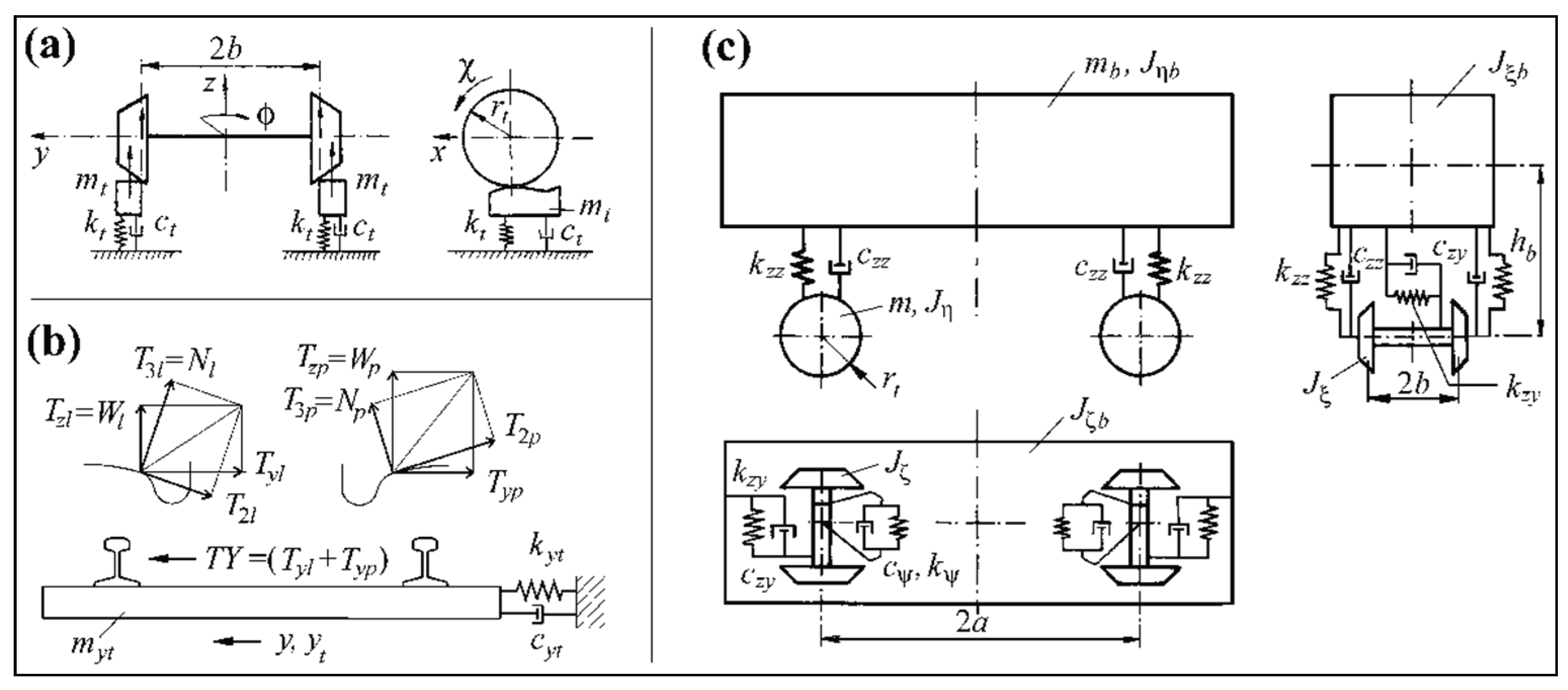
The track's models are presented in Figure 1a,b. The introduced nominal model of the vehicle is shown in Figure 1c. The full vehicle-track system has its origin in [7]. In this work, the numerical parameters of the vehicle are also presented and widely discussed.

In the proposed model, the complete dynamics of the vehicles are utilized to evaluate selected parameters of railway transitions. The behavior of a complete vehicle-track system, which needs a thorough understanding of how vehicles interact with the railway track, remains relatively uncommon even today. The concept of depicting the entire railway vehicle as a mathematical point is inadequate today. The straightforwardness of such a model renders a comprehensive analysis of vehicle dynamics unfeasible.

The complete vehicle-track model allows for the improved assignment of dynamical characteristics of railway track transitions to cargo or passenger trains. The outlined method will encompass methods for evaluating transitions beyond just the comfort of the passengers. For cargo trains, the crucial factor may be the deterioration at the wheel-rail interface.

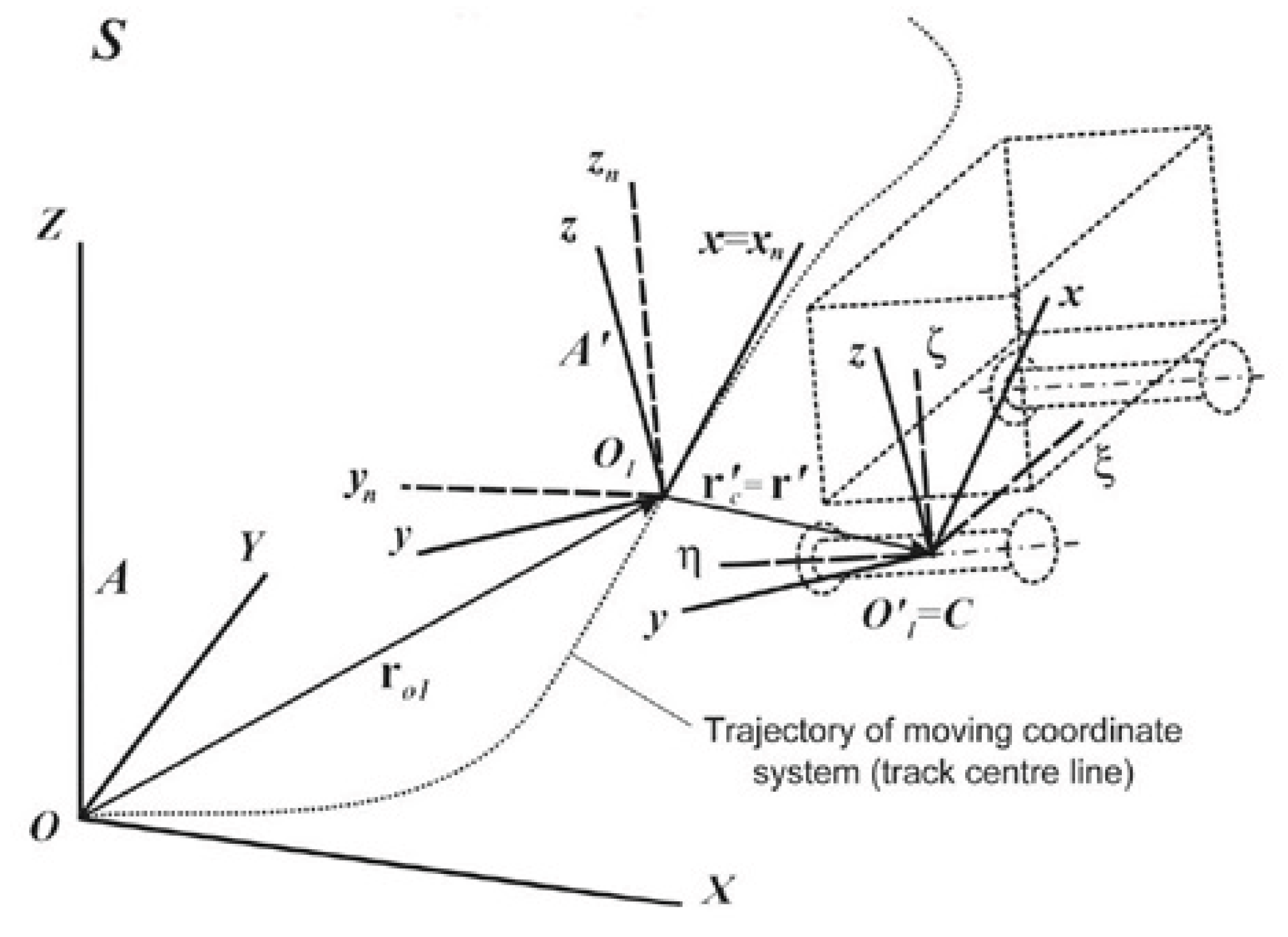
The TC shape modeling was widely described in [1]. Relative motion dynamics were a base in this approach. The vehicle dynamics was defined relative to the track-based reference frame 0₁xyz presented in Figure 2. Geometrically, model of the track was always considered laterally and vertically.

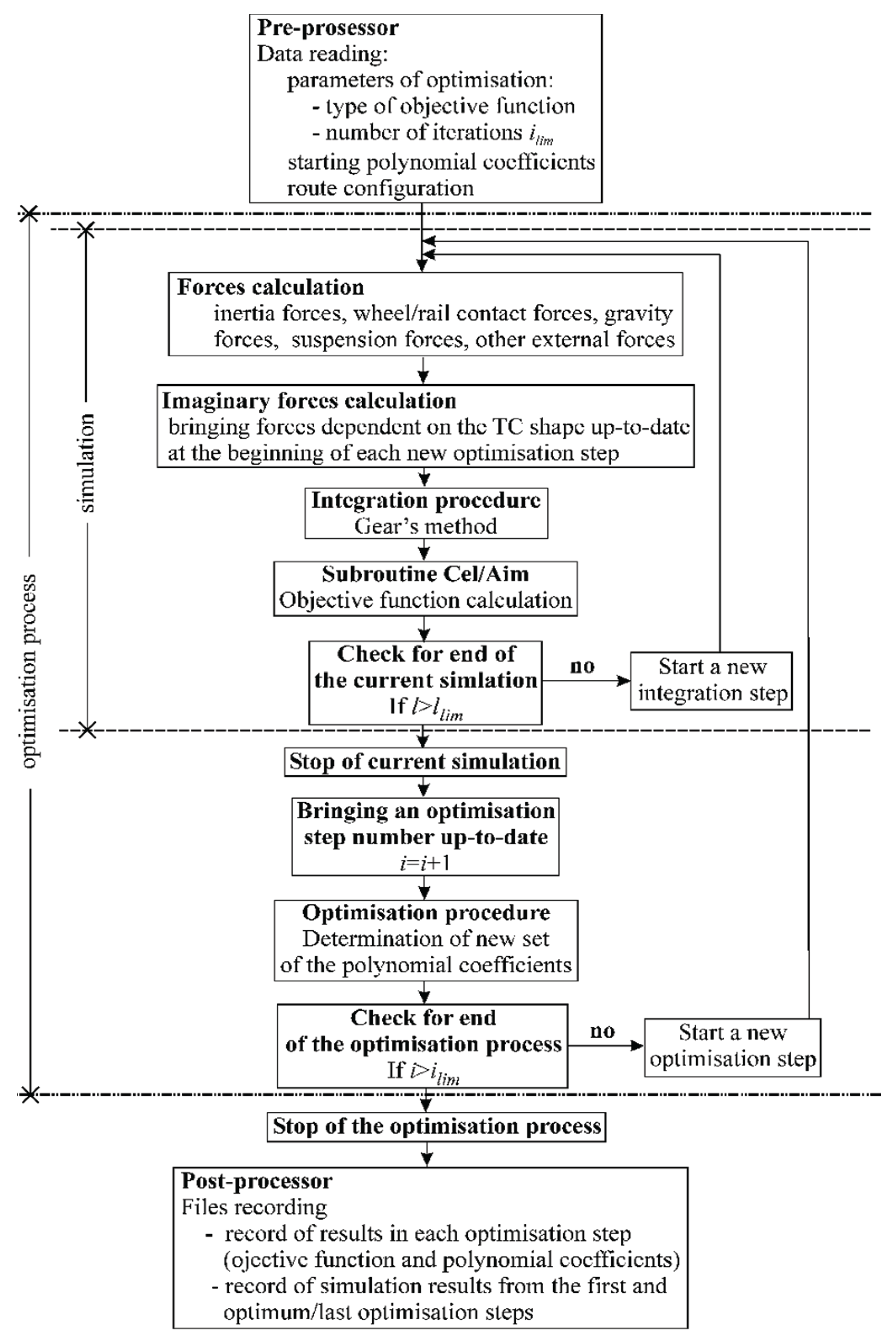
The algorithm used in the software has a relatively simple construction and is shown in Figure 3. In it, two iteration loops – integration and optimization – do their tasks, as assumed. The work of integration loop came to the end, when the vehicle model covered the declared value L_C. The optimization loop stopped working, when the value of the iterations reached the assumed limit value. The optimum solution, however, could be found earlier. Typically, such solutions were found in 50 to 250 iterations. The standard calculation time did not exceed one hour for the optimization with “normal” vehicle velocities, however, it lasted up to 2-3 days for the small velocities.

5. Results of the Simulation and Optimization

5.1. Optimization of Long Transition Curves

This chapter, as mentioned earlier, shows the results of the optimization of railway transition curves of the 9^th and 11^th degrees performed by the current work's authors. The final results were always composed of:

-

shapes of transition curves and corresponding curvatures,

-

image of railway vehicle dynamics represented by the full set of displacements, velocities, and accelerations of all main vehicle components with respect to all possible axes,

-

creepages occurring in a contact between wheel and rail.

In the optimizations performed, the routes L_c of the vehicle passage (used in formula (4)) always, as mentioned, composed of:

-

section of straight track ST, equaled to 50 m,

-

section of transition curve TC, spanned between straight and curved track,

-

section of circular arc (curved track) CA, equal to 100 m.

Table 1 shows track parameters, lengths of TCs, and velocities applied in optimization process for two analysed degrees of the polynomial—the 9^th and the 11^th. The mentioned track parameters were:

-

the radius of circular arc R [m],

-

the track cant H [mm].

Different values of R and H were applied, in general.

The 13 cases shown in Table 1 related only to those ones, when the curve length was greater than 110 m. In all these cases presented, the improvement of railway vehicle dynamics, as mirrored in smaller values of the QF₁, was a fact. The railway model negotiating the optimum transition curves had a chance to improve crucial dynamical features like body displacements and accelerations, both lateral, vertical, and angular. This statement can be fundamental for passenger comfort during the journey.

Analysing the optimizations performed, the new and practical outcomes may be defined. Firstly, the optimum transition curves obtained with smooth curvatures (condition G₁) are better than those with non-smooth curvatures (condition G₀) for the applied criterion QF₁. Therefore, the bends in the curvatures of long curves at the extreme points seem to have a negative impact on the dynamics of a vehicle travelling on such curves.

Secondly, for great TC lengths (above 120 m), the optimum polynomial TCs (for both conditions, the G₀ and G₁, and both degrees, the 9^th and 11^th) are significantly better than the cubic parabola. This can be explained just by not only greater lengths but also higher polynomial degrees (many A_i coefficients), making such curves more flexible.

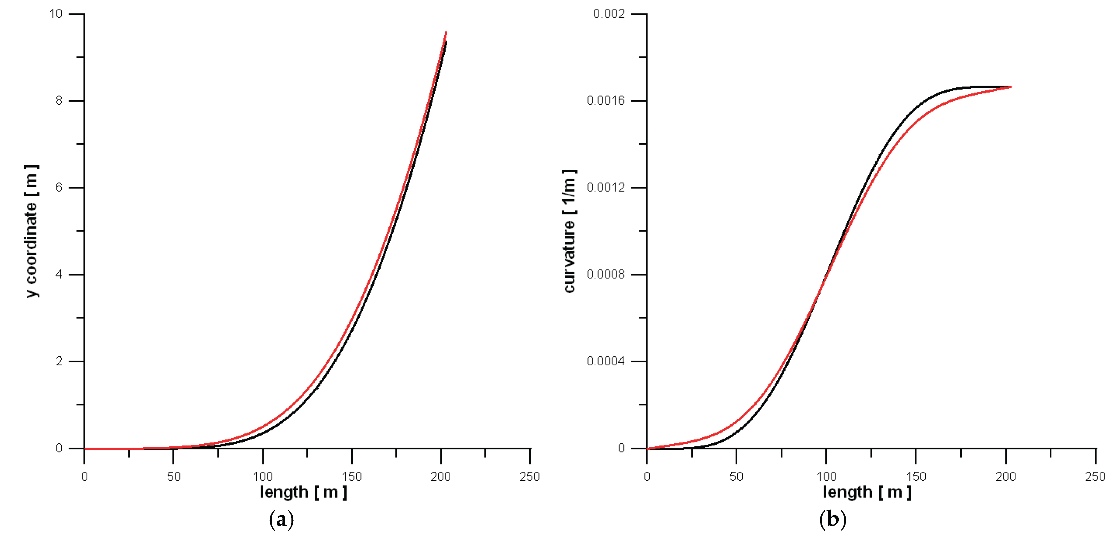
Case no. 8 from Table 2 was chosen to show the graphical results of the optimization. Figure 4a compares the TCs (represented by the y coordinate)—the starting (black), and the optimum (red), whereas Figure 4b shows the corresponding to them curvatures. It is obvious that the shape of the curvature of the newly found TC is rather closer to the standard TC of the 11^th degree (2) than to the linear curvature of cubic curve.

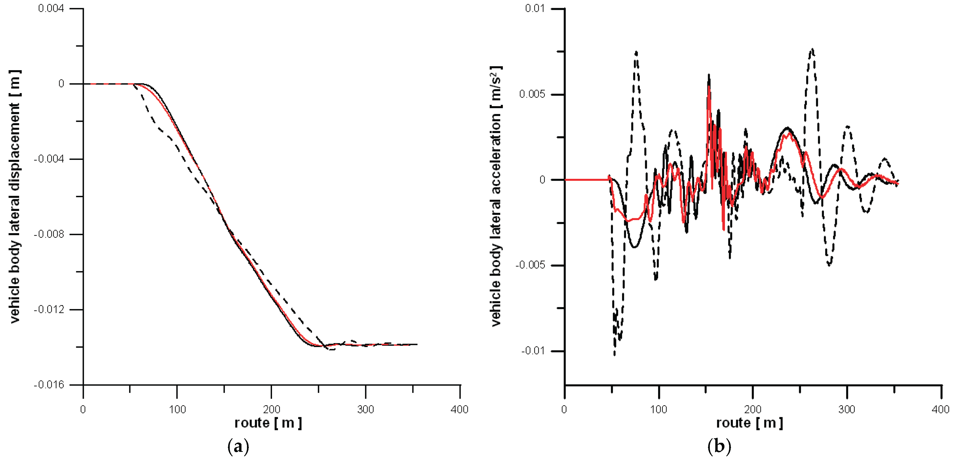
Figure 5 compares the lateral displacement and acceleration of the body mass centre for three curves:

-

initial one (black),

-

the 3^rd degree parabola (dashed), described in the further part,

-

the selected (optimum) curve (red).

Both the displacements (Figure 5a), and the accelerations (Figure 5b) prove the superiority of the newly found curve over the starting (1) and the cubic curve. In this light, what is worth noting, Figure 5b is more interesting. The unfavorable course for cubic curve clearly shows, why this curve should not be used.

Table 2 presents the numerical results of the simulations – the number of steps needed to identify the optimum curve, and the ratio of QF₁ for this optimum solution (curve) (OC) to the value of QF₁ for the starting curve (IC).

5.2. Simulation and Optimization for Small Vehicle Velocity

The present subsection aims to supplement the results from subchapter 5.1. Subchapter 5.2 presents the simulation results of the dynamics of the railway vehicle and optimization of the railway track transitions for the vehicle passing through the assumed route (ST, TC, CA) with a small velocity of 1 m/s. The 3^rd degree parabola and Bloss curve for a single passage were applied in this chapter. This was done since these curves have “normal” (not elongated) lengths. The formulas for the y coordinates of these TCs are:

$$y={\displaystyle \frac{l^3}{6R{l}_o}},$$

(5)

$$y={\displaystyle \frac{1}{R}}\left(-{\displaystyle \frac{l^5}{10l_0^3}}+{\displaystyle \frac{l^4}{4l_0^2}}\right)$$

(6)

Table 3 presents assumed parameters for the 3^rd and 5^th degrees.

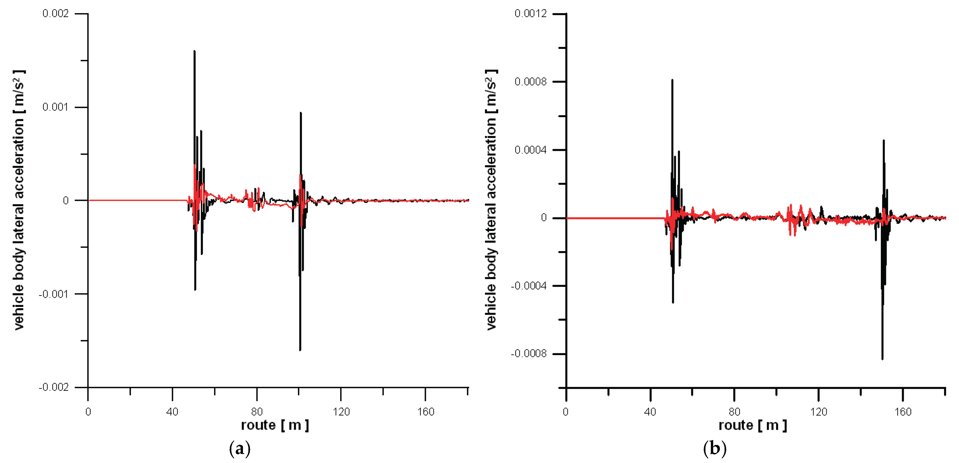
So, four simple cases - differentiated in terms of cant and curve length and represented by Figure 6 - were simulated in this part of the work.

Recalling Figure 6, one can see that the simulation results were restricted to the demonstration of the lateral accelerations of the body mass centre of the vehicle model negotiating the curves (5) and (6), earlier defined. Black line related to the 3^rd degree parabola, and red line to the Bloss curve (6).

The results of the analysis show explicitly that the Bloss curve was more favorable than the curve (3) for the considered cases. Milder transitions between the adjoining segments of the track are rather obvious. Significantly smaller peaks for the entry and exit zones (the extreme points) of the TCs are only confirmation of this observation.

Such promising results encouraged the authors to perform some optimization processes to check what transition curve of the 5^th degree can be obtained in cases, when the initial curve will be the 3^rd degree parabola. The aim of the second part of subchapter 5.2 was, therefore, to test whether the smooth curves would be found by the optimization procedure in this process.

Table 4 presents the values of the parameters of the example optimizations.

In Table 5, the numerical results of the optimization were presented.

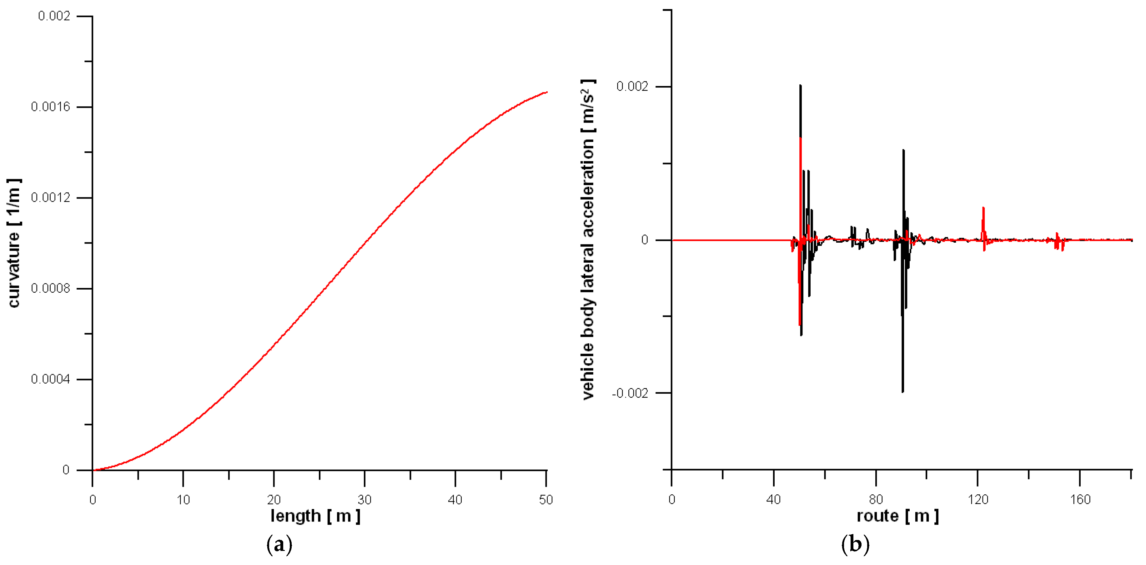
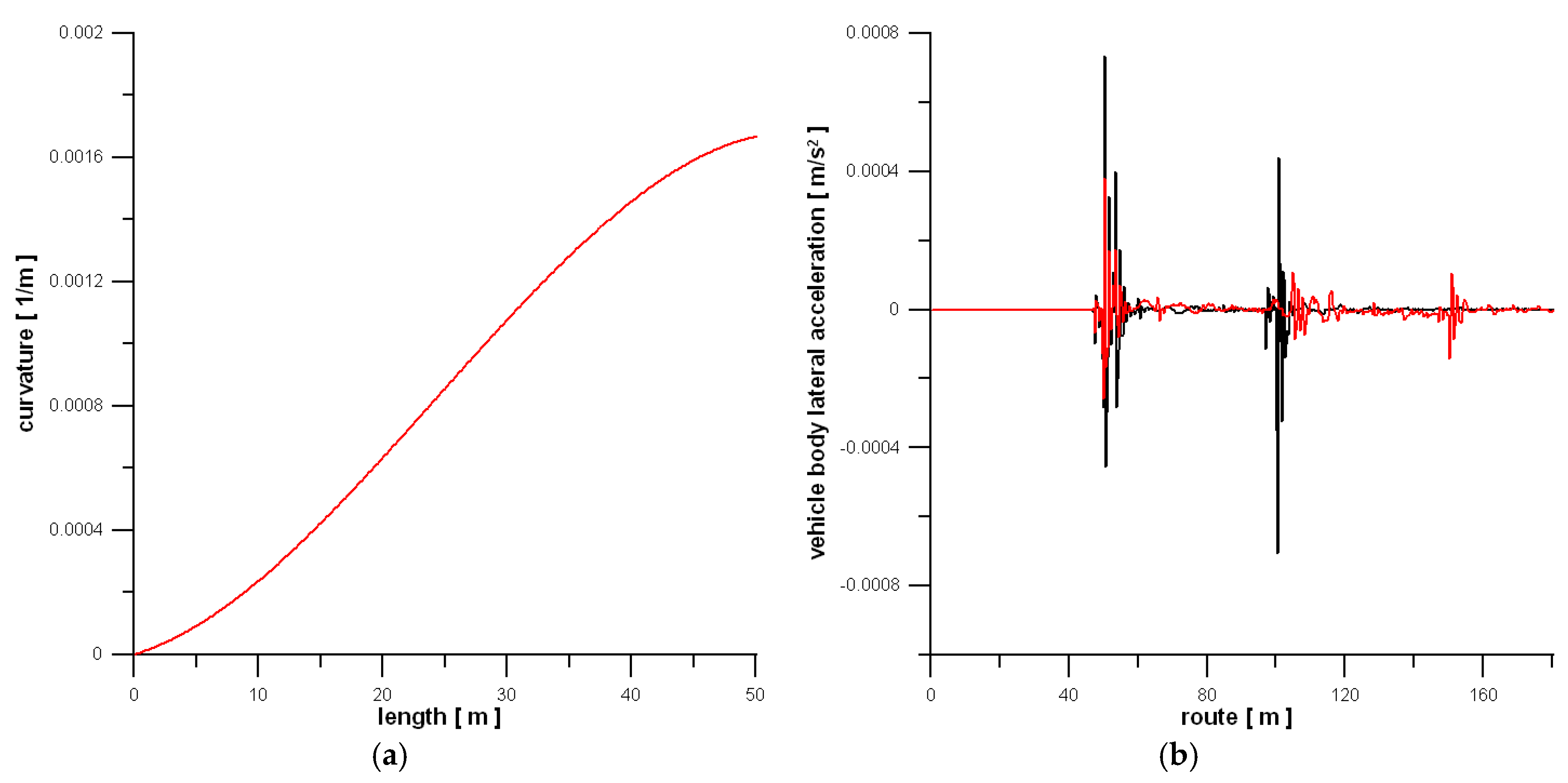
The cases (1) and (2) from Table 4 are presented visually in Figure 7 and Figure 8. The outcomes were restricted to the demonstration of the optimum curvatures and corresponding lateral accelerations of the body mass centre of the vehicle model. Peaks for the accelerations courses at the extreme curve points are visible for all cases, but these are significantly smaller, as previously, for the optimum curves (red line).

The addition to the results shown in the point 5.2, let be two Figures presenting decreases in the QF₁ values versus:

-

the iterations (steps) needed to find the optimum solution,

-

the current distance (route) covered by vehicle.

As the illustrative example, both cases from Table 5 were taken.

In the first case, the optimum solution has been found in the 98^th step, as indicated. Figure 9a shows the change in QF₁ versus the consecutive iterations (steps). A downward trend is visible, and the minimum QF₁ value was 0.0000274 [m/s²].

Figure 9b presents case no. 2 and the change in QF₁ versus the overall distance covered by the model. The last (141^st) step of the optimization is analysed, and a values decline is also visible. Since the accelerations of the vehicle become smaller and smaller in circular arc (see e.g. Figure 5b), the values of QF₁ approach relatively a fixed value. Thus, the QF₁ can be modelled by a hyperbolic function from this moment.

6. Conclusion

The work, in a simple way, verified the hypothesis concerning the bends of the curvatures of the railway transition curves in the extreme points of the curve. The authors of the work formulated the hypothesis that the time to negotiate the curve is the factor that influences the existence of the bends in the extreme points of TCs, mostly.

The results presented in the work, done with the use of a 2-axle railway vehicle, clearly showed that this hypothesis turned out to be true. It was shown that the new shapes of the optimum transition curves got for a specific arc and a long time while negotiating the curve are close to smooth curves, i.e., the bands at their extreme points are much lower than for cubic parabola and the optimum curves of the 5^th and 7^th degrees obtained in the earlier studies. So, a long negotiation time is a factor that can smooth the curvature at the extreme points. However, it is not specified how long the time must be to negotiate the whole curve.

The lack of bends (formally, the milder bends) at the curve's curvature extreme points resulted in milder courses mirrored first of all by displacements and accelerations of the vehicle body in the mentioned points. It was the most visible in the curve extremities, but also in the middle part of the curve.

It is also worth noting that the simulations and optimizations were possible even with such a small vehicle velocity equal to 1 m/s. The problem was, however, the long time needed to perform the optimizations, caused by the integration procedure. In such circumstances, the optimization calculations took approximately 2-3 days.

Since the case with small velocity could not be met in practice (trains do not operate at such speeds), the only possibility to use the railway transition curves with no curvature bends is in cases with great lengths. Such curves should be used mainly in railway lines dedicated to high-speed trains, where the curve lengths reach the greatest possible lengths.

To date, no works have shown in which situation non-smooth transition curves (having bends at curvature extreme points) are better than those with no bends. Many works focused on the TC’s shape optimization, but the need for the existence of smoothness at extreme points is still not fully explained. Thus, this work's novelty is that it possesses such an explanation. The results obtained might suggest that the use of the smooth TCs is reasonable and beneficial when their lengths are long enough, while their use for short TCs is not.

References

- Zboinski, K.; Woznica, P. Combined use of dynamical simulation and optimisation to form railway transition curves. Veh. Sys. Dyn. 2018, 56, 151–181. [Google Scholar] [CrossRef]
- Zboinski, K.; Woznica, P. Optimum railway transition curves – method of the assessment and results. Energies. 2021, 14. [Google Scholar] [CrossRef]
- Esveld, C. Modern Railway Track; MRT-Productions, 2001.
- Tari, E.; Baykal, O. A new transition curve with enhanced properties. Can. J. Civ. Eng. 2005, 32, 913–923. [Google Scholar] [CrossRef]
- Hasslinger, H. Measurement proof for the superiority of a new track alignment design element, the so-called "Viennese Curve". ZEVRail,.
- Long, X.Y.; Wei, Q.C.; Zheng, F.Y. Dynamic analysis of railway transition curves. Proc. IMechE Part F J. Rail Rap. Tr. 2010, 224, 1–14. [Google Scholar] [CrossRef]
- Zboinski, K. Dynamical investigation of railway vehicles on a curved track. Eur. J. Mech. A-Solids. 1998, 17, 1001–1020. [Google Scholar] [CrossRef]
- Zboinski, K. Numerical studies on railway vehicle response to transition curves with regard to their different shape. Arch. Civil. Eng. 1998, 44, 151–181. [Google Scholar]
- Zhang, J.Q.; Huang, Y.H.; Li, F. Influence of transition curves on dynamics performance of railway vehicle. J. Traff. Transp. Eng. 2010, 10, 39–44. [Google Scholar]
- Li, X.; Li, M.; Wang, H.; Bu, J.; Chen, M. Simulation on dynamic behaviour of railway transition curves. Proc. of ICCTP 2010, 3349–3357. [Google Scholar]
- Basak, A.; Nowak, E. Dynamics of railway vehicles movement on transition curves. Adv. In Sc. and Tech. Res J. 2021, 15, 21–29. [Google Scholar] [CrossRef]
- Xu, Y.L.; Wang, Z.L.; LI, G.Q.; Chen, S.; Yang, Y.B. High-speed running maglev trains interacting with elastic transitional viaducts. Eng. Struct. 2019, 183, 562–578. [Google Scholar] [CrossRef]
- Liu, X.; Shi, J.; Dai, J.; Wang, J.; Lu, C. Correspondence between alignment wavelength and vehicle response wavelength of high-speed rails. Int. J. of Str. Stab. and Dyn. 2025, 25. [Google Scholar] [CrossRef]
- Kufver, B. Optimisation of horizontal alignments for railway—Procedure involving evaluation of dynamic vehicle response. R. Inst. Technol. 2000. [Google Scholar]
- CEN Railway applications—ride comfort for passengers—measurement and evaluation. Brussels: ENV 12299, 2009.
- Sanchez-Reyes, J.; Chacon, J. Nonparametric Bezier representation of polynomial transition curves. J. Surv. Eng. 2018, 144. [Google Scholar] [CrossRef]
- Kobryn, A.; Stachera, P. S-shaped transition curves as an element of reverse curves in road design. The Balt. J. of Road and Bridge Eng. 2019, 14, 484–503. [Google Scholar] [CrossRef]
- Ziatdinov, R. Family of superspirals with completely monotonic curvature given in terms of Gauss hypergeometric function, Comp. Aid. Geom. Des. 2012, 29, 510–518. [Google Scholar] [CrossRef]
- Levent, A.; Sahin, B.; Habib, Z. Spiral transitions. Appl. Math. – A J. of Chin. Univ. 2018, 33, 468–490. [Google Scholar] [CrossRef]
- Pirti, A.; Yucel, M.A.; Ocalan, T. Transrapid and the transition curve as sinusoid. Teh. Vjesn. 2016, 23, 315–320. [Google Scholar]
- Shebl, S.A. Geometrical analysis of non-linear curvature transition curves of high speed railways. Asian J. Curr. Eng. Maths. 2016, 5, 52–58. [Google Scholar]
- Arslan, A.; Tari, E.; Ziatdinov, R.; Nabiyev, R. Transition curve modeling with kinematical properties: research on log-aesthetic curves. 11Comp-Aided Des and Appl. 2014, 11, 509–517. [Google Scholar] [CrossRef]
- Kobryn, A. New solutions for general transition curves. J. of Surv. Eng. 2014, 140, 12–21. [Google Scholar] [CrossRef]
- Kobryn, A. Universal solutions of transition curves. J. of Surv. Eng. 2016, 142. [Google Scholar] [CrossRef]
- Koc, W. Identification of transition curves in vehicular roads and railways. Log. and Trans. 2015, 28, 31–42. [Google Scholar]
- Koc, W. New transition curve adapted to railway operational requirements. J. Surv. Eng. 2019, 145, 145. [Google Scholar] [CrossRef]
- Koc, W. Transition curve with smoothed curvature at its ends for railway roads. Curr. J. Appl. Sci. Techn. 2017, 22, 1–10. [Google Scholar] [CrossRef]
- Fischer, S. Comparison of railway track transition curves types. Poll. Period. 2009, 4, 99–110. [Google Scholar]
- Barna, Z.; Kisgyorgy, L.J. Analysis of hyperbolic transition curve geometry. Period. Polytech. Civil. Eng. 2015, 59, 173–178. [Google Scholar] [CrossRef]
- Shen, T-I. ; Chang, C.H.; Chang, K.Y.; Lu, C.C. A numerical study of cubic parabolas on railway transition curves. J. Mar. Sc. Tech. 2013, 21, 191–197. [Google Scholar]
- Eliou, N.; Kaliabetsos, G. A new, simple and accurate transition curve type, for use in road and railway alignment design. Eur. Trans. Res. Rev. 2014, 6, 171–179. [Google Scholar] [CrossRef]
- Sadeghi., J.; Rabiee, S.; Khajehdezfuly, A.; Felekari, P. Sadeghi., J.; Rabiee, S.; Khajehdezfuly, A.; Felekari, P.: Investigation on optimum lengths of railway clothoid transition curves based on passenger ride comfort. Proc. IMechE Part F J. Rail Rap. Tr 2022, 237. [Google Scholar]
- Temirbekov, E.S.; Bostanov, B.O.; Dudkin, M.V.; Kaimov; S. T. Kaimov, A.T.: Combined trajectory of continuous curvature. Adv. In Ital. Mech. Sci. 2018, 12–19. [Google Scholar]
- Brustad, T.F.; Dalmo, R. : Railway transition curves: a review of the state-of-the-art and future research. Infrastr. 2020, 5. [Google Scholar] [CrossRef]
- Casal, G.; Santamarina, D.; Vazquez-Mendez, M. Optimization of horizontal alignment geometry in road design and reconstruction. Transp. Res. Part C: Emerg. Technol 2017, 74, 261–274. [Google Scholar] [CrossRef]
- Tasci, L.; Kuloglu, N. Investigation of a new transition curve. The Balt. J. of Road and Bridge Eng. 2011, 6, 23–29. [Google Scholar] [CrossRef]
- Ciampa, D.; Olita, S. : The use of Bloss curve in the exit lanes of road intersections. The Balt. J. of Road and Bridge Eng. 2020, 15. [Google Scholar] [CrossRef]
- Ciampa, D.; Diomedi, M.; Vouno, P.; Olita, S. : The use of transition curves in airport runway rapid exit taxiways (RETs). Adv. In Civ. Eng. 2024, 460968. [Google Scholar] [CrossRef]