
Submitted:
01 October 2025
Posted:
02 October 2025
You are already at the latest version
Abstract
This paper presents numerical simulation results on the nonlinear features of railway vehicles moving in transition curves at velocities close to the critical velocity. It examines six objects representing railway vehicles: three 2-axle bogies, two 2-axle freight cars, and a 4-axle passenger car. The paper aims to show how systematic variation of motion conditions, such as initial conditions, vehicle velocity, and curve radius, influences nonlinear features of the vehicle’s dynamics. Results indicate that initial conditions do not affect stable solutions, increasing velocity leads to more systematic patterns of behaviour across straight, circular, and transition curves, while increasing curve radius leads to a partly systematised picture of solutions. The findings also emphasise certain exceptions to these general trends.
Keywords:
nonlinear phenomena
; vehicle dynamics
; transition curve
; lateral stability
; raivay vehicle
; critical velocity
1. Introduction
The introduction should briefly place the study in a broad context and highlight why it is important. It should define the purpose of the work and its significance. The current state of the research field should be carefully reviewed and key publications cited. Please highlight controversial and diverging hypotheses when necessary. Finally, briefly mention the main aim of the work and highlight the principal conclusions. As far as possible, please keep the introduction comprehensible to scientists outside your particular field of research. References should be numbered in order of appearance and indicated by a numeral or numerals in square brackets—e.g., [1] or [2,3], or [4,5,6]. See the end of the document for further details on references.
The paper investigates the nonlinear dynamics of railway vehicles negotiating transition curves at velocities v around the nonlinear critical velocity vn, including velocities below and above. The primary focus is on the lateral dynamics of vehicles in transition curves (TC), with references to straight track (ST) and circular curve (CC) behaviour as comparative contexts. The study involves numerical simulations of vehicle-track system dynamics for six vehicle models representing different types of bogies and cars. Their closer profile is as follows: 25TN bogie of freight cars, the bogie with average parameters, bogie of MKIII passenger car, the unloaded 2-axle freight car of average parameters, the loaded 2-axle HSFV1 freight car, and the 4-axle MKIII passenger car of two bogies. Some models have counterparts among actual railway vehicles; nevertheless, all are treated as generic thanks to their simplicity.
The results come from the research project mentioned in the acknowledgements section of this paper. The project’s partial results for the unordered behaviours have already been published [35]. In this paper, the results recognised as ordered are of primary interest. The unordered and ordered results’ aspects were equally important in the authors’ earlier publications [6,7,35,54].
The main objective of the present paper is to continue to enlighten, highlight and expand the knowledge of practitioners and theoreticians on highly nonlinear features of railway vehicles in TCs and their vicinity at velocities close to the nonlinear critical velocity vn. Considering the present authors’ results and the sporadic publications on that topic by others, this knowledge is still low. The objective, as stated, is hard to achieve without publishing all the relevant results based on the 3,000 simulations, approximately. Only this can enlighten the audience about the nature and scale of the issue. It is hard to do in a single paper, so the need for the present paper is clear.
The authors focus on presenting the nonlinearities they found, regardless of the motion conditions. That is why the last ones are scattered and do not necessarily correspond to conditions in the real railway system. Also, the reasons or insights into the disclosed nonlinear phenomena are limited. Those unexplained would require hundreds of profiled simulations. Thus, the authors do not intend to provide clear guidance for the engineering industry at the present stage.
Instead, the new theory can be explicitly formulated for the first time in the present paper. It states that, considering the already tested six generic vehicles and three existing vehicles and the nonlinearities in TC and its vicinity at velocities close to vn found for all these objects, such a type of nonlinearities is the inherent feature for all the railway vehicles guided based on the wheel-rail (wheelset-track) contact.
The contribution of the present paper to the main objective is achieving a more detailed aim, referring to part of all the results obtained. It examines how systematic variations in motion conditions, such as initial conditions y(0), velocity v, and curve radius R, affect vehicle behaviour in TC, which is difficult to predict based on the behaviour in ST and CC. The completion results to be published next are those considering the influence of suspension parameters on the nonlinear behaviour for the generic vehicles and the unpublished results for the existing vehicles.
1.1. Supplementary Information
The topic relates to the bifurcation approach to lateral stability of rail vehicles. The relation is by the vn notion, and the simulation software, a numerical tool in such studies. One should be aware that stable periodic vibrations are possible for ST and CCs as constant motion conditions exist. It is not so for TC, where track curvature and superelevation change continuously. Thus, stable periodic or stationary solutions cannot be expected or searched for in TC, identically as the vn. Despite these, any non-stationary and non-periodic solution can be examined for its stability. However, such a formal examination for the stability of solutions in TC has never been seen so far. Such stability analyses for ST and CCs, by other and present authors, can be found in e.g. [18,19,20,21,22,23,24,41,48] and [25,35], respectively.
As mentioned, the reason for undertaking the topic is the low cognisance of rail vehicles’ strongly nonlinear behaviour in TC and its vicinity at v around vn. The knowledge gained would hopefully bring practical benefits to vehicle construction and motion safety. The findings connecting stability and safety can be an example. Valuable would be the comprehension when vibration amplitudes in TC are bigger than in ST and CCS, and when vibrations vanish in TC despite their existence in ST and CC. It could contribute to vehicle construction, to eliminate the first feature (undesired state) and ensure the second (desired state).
1.2. The Literature Survey
It is hard to find a more significant number of publications by others where the topic of interest is treated directly, e.g. [1,2,3,4,42]. Examples of the present authors’ publications are [7,8,35,54].
The motivational publications are [1,2,3,4,5], where the results for TCs were generated at the stability study in ST and CCs. Concerning vehicles, a 2-axle freight car [1,2], a 4-axle heavy-haul vehicle [3], a 4-axle passenger car [4], and two bogies and two 2-axle freight cars [5] were of interest. In [1,2], behaviour in TC is a logical passage from periodic vibrations in ST to those in CC. However, perturbations in regular behaviour in TC and CC exist, caused by the non-smoothness of dry friction in the suspension. In [3], the absence of vibrations in ST, their start and development in the middle of TC length, and then continuation in CC as a limit cycle are interesting. In [4], no vibrations appear in ST. They begin immediately in TC and continue as a limit cycle in CC. In [5], the behaviour in TC usually makes a logical passage from limit cycles in ST to those in CC. However, three intriguing cases were disclosed. The first is the entire disappearance of vibrations in TC, despite limit cycles in ST and CC. The second is no vibrations in ST and TC, and their appearance after entering CC, however, for the leading wheelset only. The third is the vibrations from fundamental change (amplitude and frequency) in the middle of TC. Common in [1,2,3,4,5] is no deliberate, systematic variation of the motion conditions or other parameters to study vehicles’ behaviour changes (nonlinear features). Some exceptions are [1,2], where results for two velocities are shown.
Considering rare publications strictly in line with the present topic, it is reasonable to indicate those where coordinate courses in TC above vn were either simulated but not published or could have been potentially obtained, e.g. [8,9,10,11,12,13,14,28,29,40]. Interesting are publications where the dynamics of the vehicle-track system is exploited to look for the proper, best, or optimum shape of TCs [15,16,17]; velocities are below vn, however. In [15], the length of parabolic TC of the 3rd order is optimised, with three dynamical criteria. In [16], six different TC are compared, while six dynamical criteria were of interest. In [17], the optimum shape of polynomial TCs of orders from 5th to 11th is searched for at eleven dynamical quality functions.
Despite dynamical, a more traditional approach remains. In [51], the new shape of smooth TC was proposed using analytical methods focused on the curve’s geometrical properties. The [52] describes a new method for designing vertical curves in the curved road/track sections. It applies a single curve connecting two STs, the so-called general TC. In [50], the result is a parametric approach to search for optimum lengths of the clothoid TC, considering passenger comfort in a curved track. In [46], an explicit interest in the presence of TC occurs. The CC radius R and TC length appeared to be key parameters, provided R ≥ 800 m and the lengths are small. The review paper [49] is impressive, discussing seventy publications about TCs. Its aspects are numerous, complete, and well-balanced. Three future research areas are defined, including the dynamical evaluation criteria with a discussion of [35], where the approach is as in the present paper.
The selected, recent publications on the stability are [36,37,38,39,41,42,43,44,45,47,48]. Luckily, the authors found at least one publication [42] by others where the vehicle dynamics on TC is shown at v>vn. A hunting motion of an electric locomotive’s car body is tested with measurements and simulations. The body and wheelset hunting appear in ST and disappear in CC. The variation in suspension parameters to overcome car body hunting is outlined. Despite jointly showing the results for TC, ST, and CCs, the authors missed the discussion for the TC entirely. Publication [36] performs the stability study of a high-speed railway (HSR) train. A new approach originating from the root loci method was effectively applied and tested. Publications [37,38] present and use nonlinear wheelset models undergoing the bifurcation analysis. In [37], the possibility of coexisting stable and unstable limit cycles is demonstrated and extended to the unfavourable behaviour of Chinese HSR trains. The [38] includes comparisons of results for linearised and nonlinear wheel-rail contact and different field-measured wheel profiles. Publication [39] introduces a method of identifying, instead of neglecting, the hunting of low amplitudes for HSR vehicles. In [41], several methods for determining vn are compared. The direct simulation, ramping, and continuation methods were of primary interest. The methods’ comparison of exciting the hunting was performed considering vn value. A novel measuring system to monitor the rail vehicles’ hunting motion is presented in [43]. The [44] is of great intellectual value. The existence of parametric vibrations in a wheelset-track system, caused by wheel load fluctuations, is disclosed and experimentally verified. Their coexistence with self-exciting vibrations can cause a resonance. In [45], a nonlinear model of wheel-rail hunting kinematics, extending Klingel’s linear model, is presented. It additionally takes account of high-order odd harmonic frequencies (HOHFs). Publication [47] is a literature review for the bogie and the car body hunting instabilities’ fault diagnosis, with the small (and moderate) amplitude hunting included. In [48], the review paper, the survey of linear and nonlinear methods of the lateral stability analysis of rail vehicles is presented and discussed (some aspects are missed, while the older ones are disproportionately widely discussed).
The above review confirms that rail vehicle dynamics in TCs at velocities close to vn is rarely undertaken. Not much has happened in recent years in this area beyond the works by the present authors. To intensify such studies, they have recently published an encouraging paper [54]..
2. Modelling Bases, Models of the Objects, and Software in the Study
2.1. The Modelling Principle
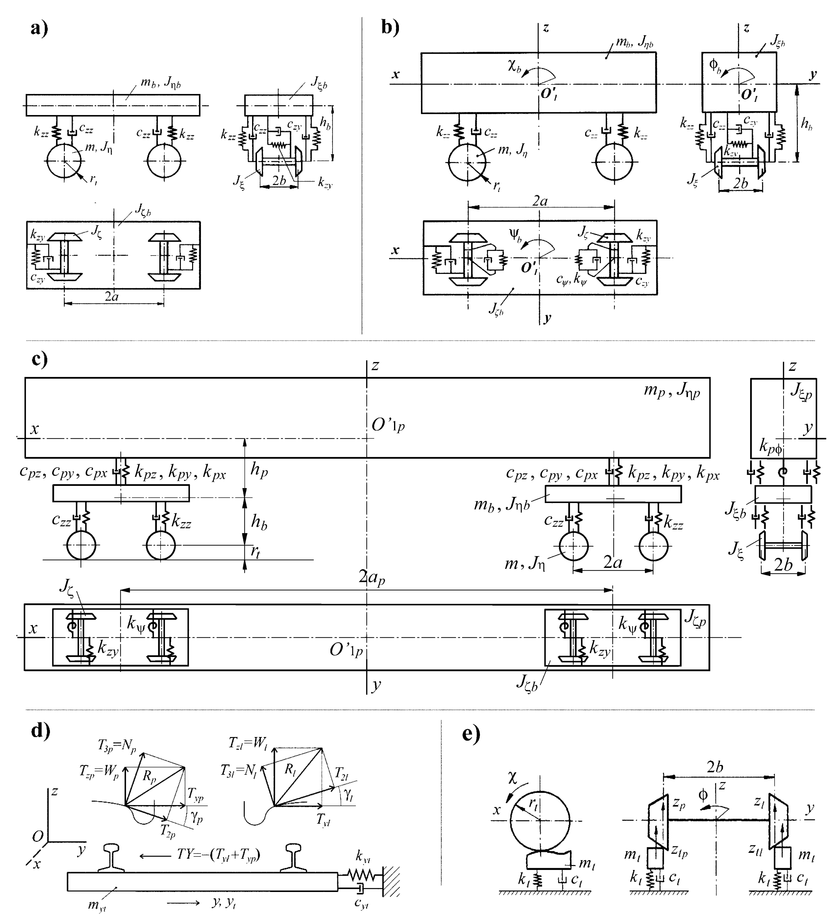
The method used for modelling the dynamics of rail vehicles is generalised, as discussed in [17,26,27,35]. The generalisation is in vehicle models, serving any motion conditions. Hence, the same equations of motion hold in TC of any type, CCs, and ST. The dynamics of relative motion, i.e. relative to track-oriented moving (non-inertial) reference systems, is applied. Hence, the explicit inertia terms (called imaginary or correction forces [30]) exist due to the moving systems. The linear and angular velocities and accelerations of transportation, i.e. of the moving systems, are the only ones needing introduction into these terms to represent the shape defined by parametric equations. The 3-D shape represents any TC with a superelevation ramp, while the 2-D and 1-D shapes represent CC and ST. Next generalisation is the validity of the modelling approach for any equations of motion. It covers equations traditionally derived and those numerically built with software for automatic generation of equations of motion (AGEM). The Lagrange equations of type II and Kane’s equations, adapted to the relative motion description, represent the above two cases in this paper.
2.2. The Objects’ Nominal Models
Each model of the six objects, supplemented with the same track models, is a set of rigid bodies, forming discrete vehicle-track systems.
The models’ structures of the laterally and vertically flexible track are shown in Figure 2d and Figure 2e, respectively. The structures of the 2-axle bogies are given in Figure 2a, while 2-axle cars are in Figure 2b. The structures of the bogie of the MKIII car, the bogie with average parameters and the 2-axle cars are identical. Their degrees of freedom (DoFs) number, incorporating the track, equals 18. The 25TN bogie-track model has 16 DoFs. The eliminated two DoFs block yaw rotations of wheelsets relative to the bogie frame. Thus, parameters kzx and czx for 25TN bogie in Table 1 remain undefined. The 4-axle passenger car structure is shown in Figure 2c. Its vehicle-track model has 38 DoFs.
Table 1 and Table 2 contain the parameters for 2-axle objects and for 4-axle car and the track, respectively. The parameters origin for the 25TN bogie, the bogie of MKIII passenger car, the freight cars HSFV1 and of average parameters, and the track is [5]. The source for the bogie with average parameters and the MKIII passenger car is [35]. Vertical load for the 25TN and average parameters bogies arises from half of the 4-axle vehicle body mass (12 300 kg). The respective mass for the bogie of MKIII car is given in Table 2.
2.3. The Simulation Software
Three proprietary programs enabled motion simulation for the tested objects. The first served: the bogie with average parameters, the bogie of the MKIII passenger car, the 2-axle freight car of average parameters, and the 2-axle HSFV1 freight car of the same DoFs number. The second served the 25TN bogie of freight cars, of different DoFs number. In the first and second programs, Lagrange formalism of type II has been used, while the equations were derived traditionally. The first use of these programs is [5]. The third AGEM-type program served the 4-axle MKIII passenger car, while Kane’s formalism has been used. It has been called ULYSSES in [36]. Its example applications for a 2-axle freight- and the MKIII cars are [35,36].
All programs exploited the same methods for wheel-rail contact. The FASTSIM program [32] generates the nonlinear tangential contact forces. The friction coefficient adopted was equal to 0.3. Nonlinear shapes of real wheel and rail profiles define the contact geometry. Contact parameters are generated by the RSGEO software [31]. The unworn (nominal) profiles S1002 and UIC60 of wheel and rail were adopted. The track gauge and rail inclination equal 1435 mm and 1:40, respectively.
The equations of motion were integrated with Gear’s method to solve stiff ordinary differential equations [33]. The integration procedure corrects the relative calculation error E automatically.
The modelling approach, models, and software are well verified. Their applications, going into the tens (e.g. [5,6,7,17,25,26,35,53,54]), made it possible to develop them for years. Many verification actions were undertaken. The accuracy of calculations was studied, e.g. in [25]. The results of the first and second, and the ULYSSES programs, were compared, and the programs were corrected until the results became the same. Verification was also a qualitative comparison of the ULYSSES and commercial VI-Rail code results for similar passenger cars [35].
3. Method of the Analysis and Characteristics of the Results
This section may be divided by subheadings. It should provide a concise and precise description of the experimental results, their interpretation, as well as the experimental conclusions that can be drawn.
The analysis method follows a straightforward four-step procedure. The first step involves simulating the vehicle’s nonlinear behaviour changes due to variations in motion conditions. The second step consists of presenting the obtained results in plots. The third step involves commenting on and explaining the results, and the fourth step is drawing conclusions.
A key element in the present study related to stability is the nonlinear critical velocity, vn. It originates from the bifurcation approach to nonlinear lateral stability of rail vehicles, being in use for many years (e.g., [21,23,34]). For rail vehicles’ systems (with many DoFs), vn can only be determined via numerical simulation. This contrasts with the linear critical velocity vc, which can also be determined analytically for systems with few DoFs. However, vc often overestimates the critical velocity, leading to an incorrect indication of the hunting onset for a higher velocity than the actual one. It reduces safety and eliminates vc as a useful measure, according to the present authors and many others. The vn. is the smallest velocity at which stable periodic solutions (hunting motion) can occur for the vehicle model (real object). The authors always refer to nonlinear critical velocity when using the term "critical velocity” and differentiate vn in ST and CCs of different radii (e.g., [6,25,26,35]).
The current paper does not present simulation results for determining vn, as this has already been described and published in [53] for all 2-axle objects and in [35] for a 4-axle vehicle. In [53], the authors classify the methods for determining vn as follows: 1) direct simulation method with limited accuracy; 2) direct simulation with high accuracy (extended method in [25]); 3) ramping method, where vn is determined in a single simulation at decreasing velocity; and 4) continuation methods, where simulations are carried out for different velocities, with the previous results used as initial conditions for the current simulation. The advantages and limitations of these methods are discussed in [53], where the authors justify their choice of method. They used both the first and second methods simultaneously, ensuring that jumps of solutions (bifurcations) and multiple solutions were correctly captured to determine vn.
Simulation results were obtained for successive sections of the route: ST, TC, and CC, separated in figures by vertical lines. The TC was a 3rd-degree parabolic curve, while superelevation h in CCs ensured the exact balance between gravity and centrifugal forces. When h exceeded the maximum allowed value of h=150 mm (in Poland), this maximum value was applied. Variation of the superelevation h is to be performed in further studies. At this stage, it would obscure the image of the results and make understanding the nature and reasons of particular nonlinearities harder.
Specific route data are provided in the figure captions. The suspension parameters variations, enhancing the features, are given as multiples of the nominal values in Table 1 and Table 2.
The results are time history plots of vehicle lateral dynamics coordinates, lateral displacements y and yaw angles , with additional indices b, l, and t, for bogie frame or vehicle body, front (leading) wheelset, and rear (trailing) wheelset (2-axle objects) and p, b1, b2, 1, 2, 3, and 4 for vehicle body, front bogie frame, rear bogie frame, and wheelsets (front and rear in the b1 and front and rear b2 bogies). At intensive parameters’ variations, the indices extensions referring to radii R, velocities v, and initial conditions y(0) (separated with a slash) are applied.
The initial conditions imposed concerned displacements y of all rigid bodies in the model with typical values yi(0)=0.0045 m and yj(0)=0.004 m for 2- and 4-axle objects, respectively.
4. The Impact of Initial Conditions
4.1. The 25TN Freight Car Bogie
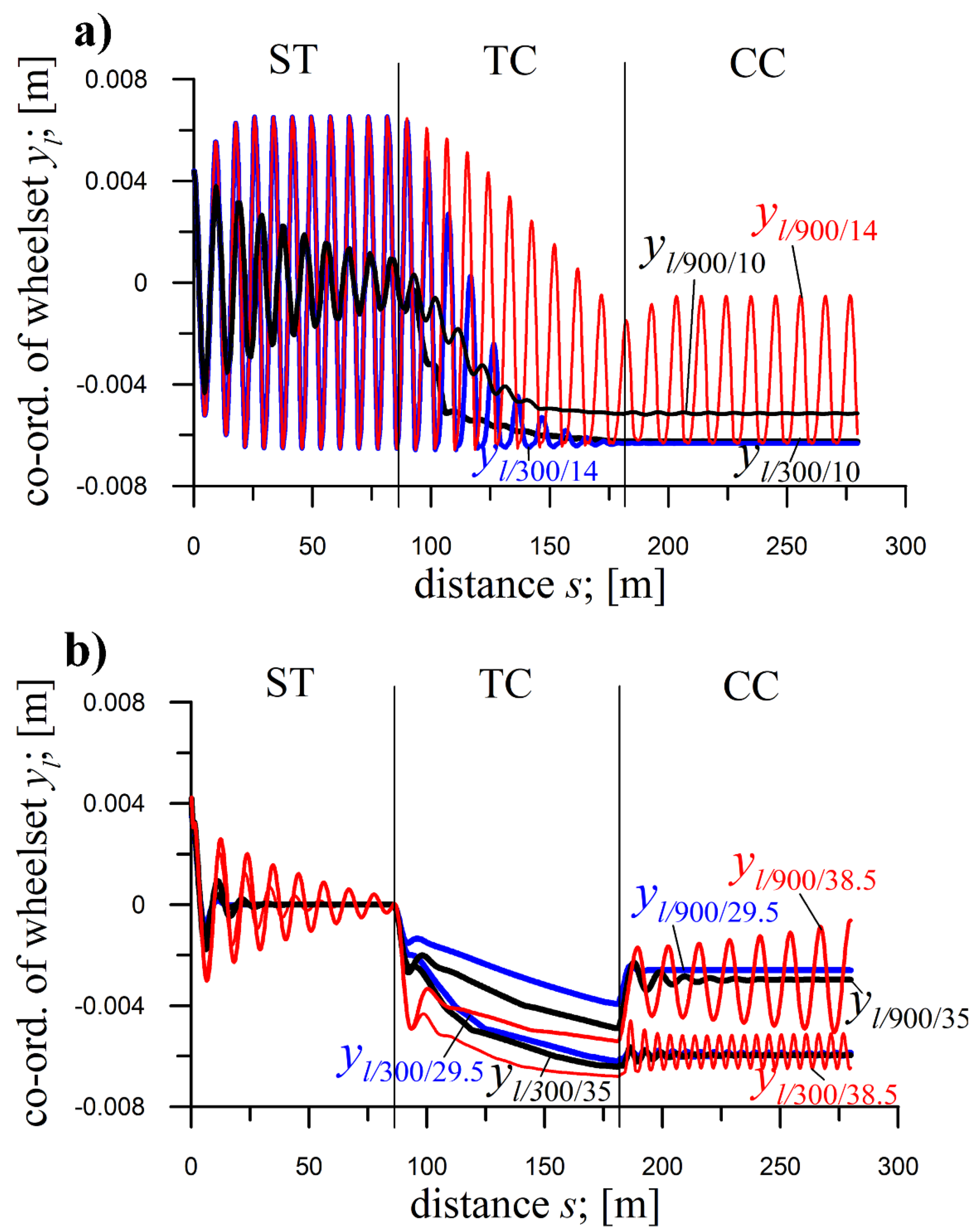
The impact of yi(0) on solutions for the 25TN bogie is illustrated in Figure 2, at integration relative error E=0.4.
At a curve radius R=900 m, comparing zero (yi(0)=0 m) and non-zero (yi(0)=0.0045 m) initial conditions reveals that the solutions in the circular curve (CC) remain unchanged. The identical periodic solutions for the front wheelset confirm that initial conditions in the straight track (ST) do not influence the behaviour in CC, aligning with the theoretical limit cycle concept.
Similarly, at R=2000 m, zero and non-zero initial conditions (yi(0)=0.0, yi(0)=0.002, and
Figure 2.
Coordinate of leading wheelset of 25TN bogie of a freight car at v=29.5 m/s and ST (l=76.6 m), TC (l=95 m), and CC (l=98 m); for: R=900 m; h=0,142 m; yi(0)=0 m and yi(0)=0.0045 m, and R=2000 m; h=0.064 m; yi(0)=0 m;yi(0)=0.002 m andyi(0)=0.0045 m yi(0)=0.0045 m) yield nearly identical solutions in CC, differing only in phase. Adjusting the length of the ST or transition curve (TC) could align these phases fully.
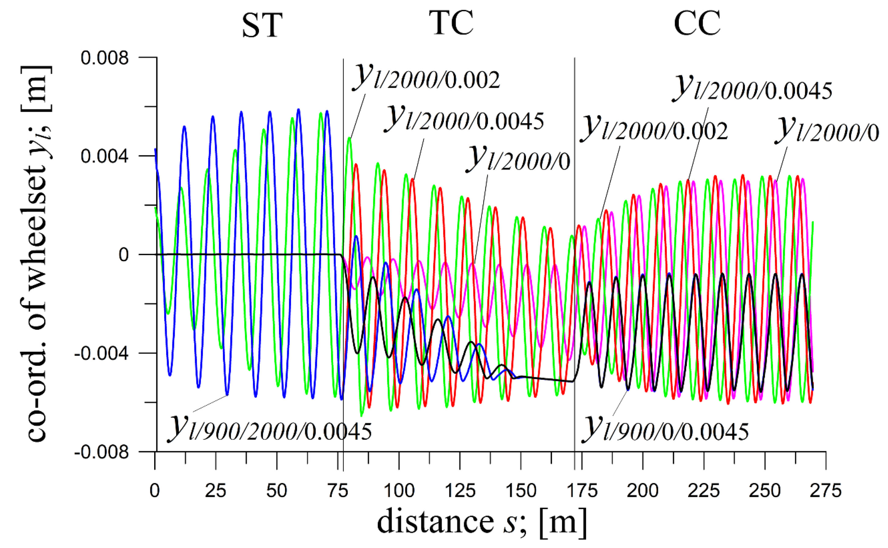
An unexpected result emerges when comparing behaviour at R=900 m and R=2000 m for zero initial conditions. At R=900 m, vibration amplitudes quickly rise in the TC, while at R=2000 m, amplitudes grow gradually. Interestingly, for non-zero initial conditions, the vibration amplitudes are higher at the start of the TC at R=2000 m than at R=900 m.
4.2. The 4-Axle MKIII Passenger Car (Initial Conditions)
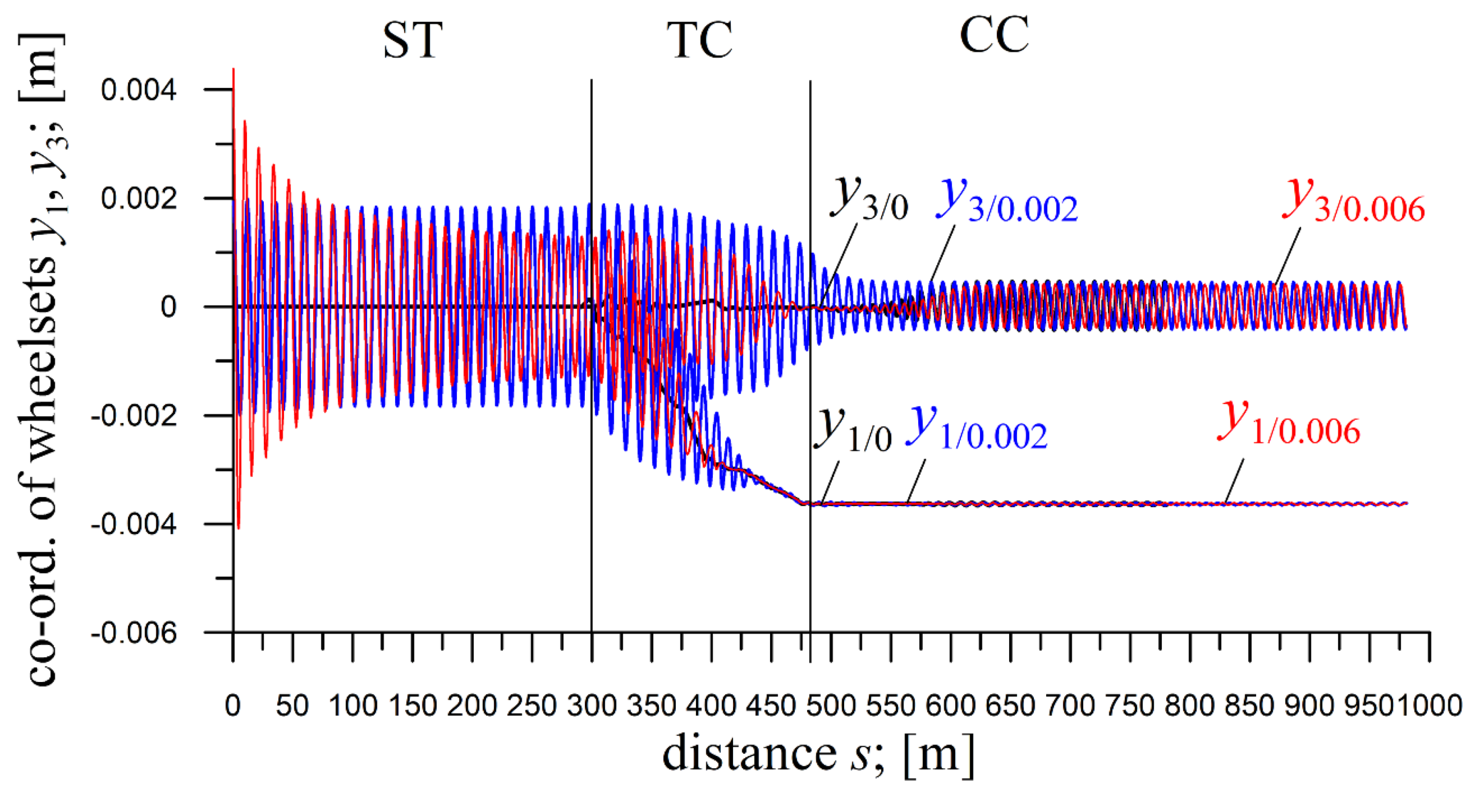
The impact of yi(0) on the solutions for the MKIII car is illustrated in Figure 3 and Figure 4, obtained at E=0.05.
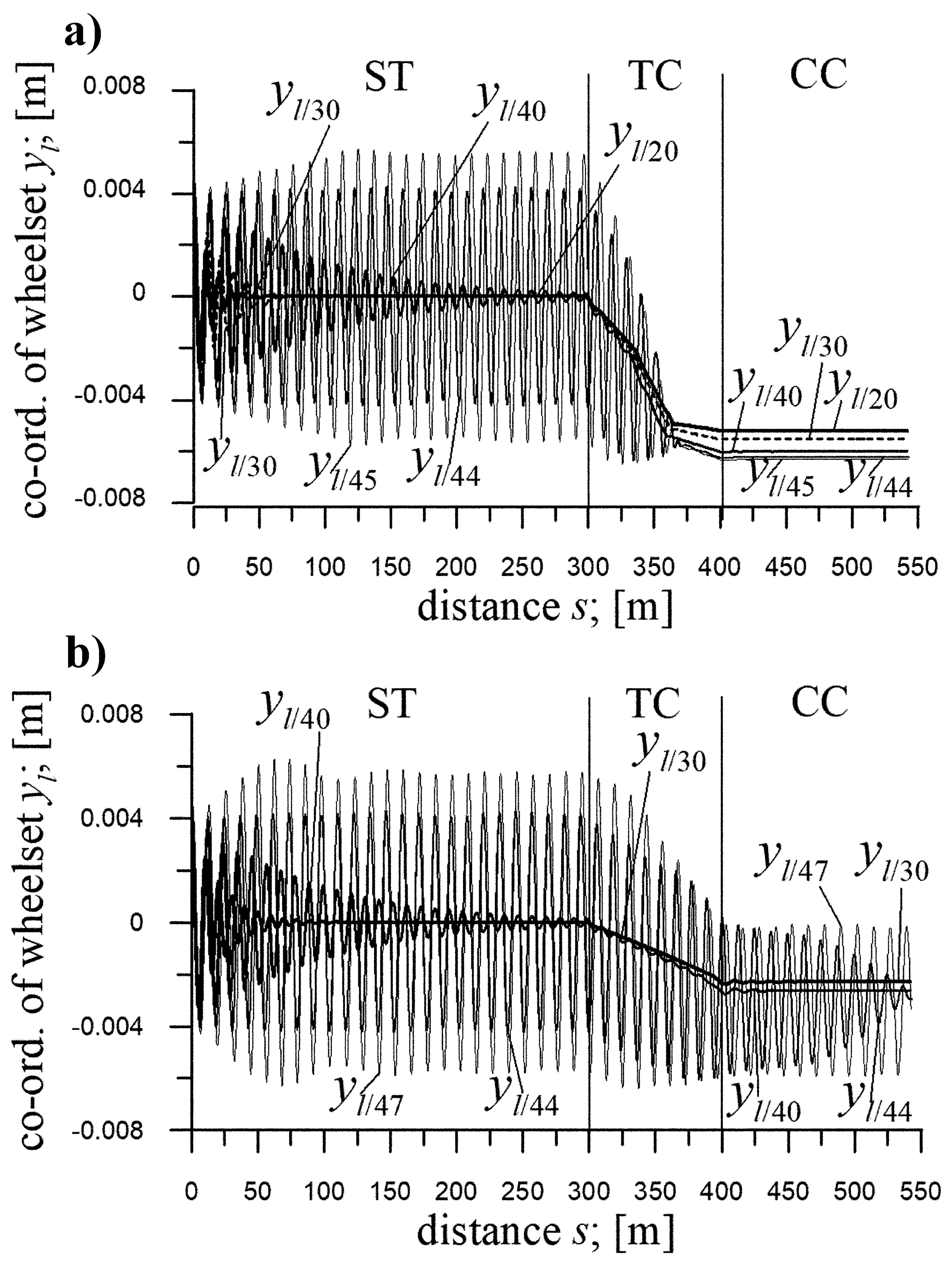
At R=600 m and velocity v=20 m/s (Figure 3), different yj(0) values (from their entire scope) do not affect the solutions in CC, which remain identical. Minor quantitative differences appear in the TC’s final part, but the qualitative behaviour is preserved. A notable feature in ST is that larger initial conditions lead to lower vibration amplitudes on entering the TC, suggesting multiple coexisting solutions – an effect previously identified in [35].
At R=600 m and v=35 m/s, and for R=1200 m at v=20 m/s (not illustrated), results follow the same pattern, with only increased leading wheelsets’ displacements in CC due to the larger v and R, respectively.
At R=2000 m and v=20 m/s (Figure 4), solutions in CC remain identical for all yj(0) values (from their entire scope), but multiple solutions in ST reappear, as at R=600 m. A peculiar observation is the delayed onset of vibrations in CC for yj(0)=0 and 0.006 m, though there are no vibrations in TC’s final part and CC’s beginning. Vibrations already exist at the CC's beginning for yj(0)=0.002 m (and not illustrated 0.004 m).
Figure 3.
Lateral displacements of wheelsets in the front bogie of passenger car MKIII for R=600 m; h=0,15 m; ST (l=150 m), TC (l=180.46 m), CC (l=100 m): at v=20 m/s; yj(0)=0 m, yj(0)=0.002 m and yj(0)=0.006 m, and at v=35 m/s; yj(0)=0 m and yj(0)=0.004 m.
Figure 3.
Lateral displacements of wheelsets in the front bogie of passenger car MKIII for R=600 m; h=0,15 m; ST (l=150 m), TC (l=180.46 m), CC (l=100 m): at v=20 m/s; yj(0)=0 m, yj(0)=0.002 m and yj(0)=0.006 m, and at v=35 m/s; yj(0)=0 m and yj(0)=0.004 m.
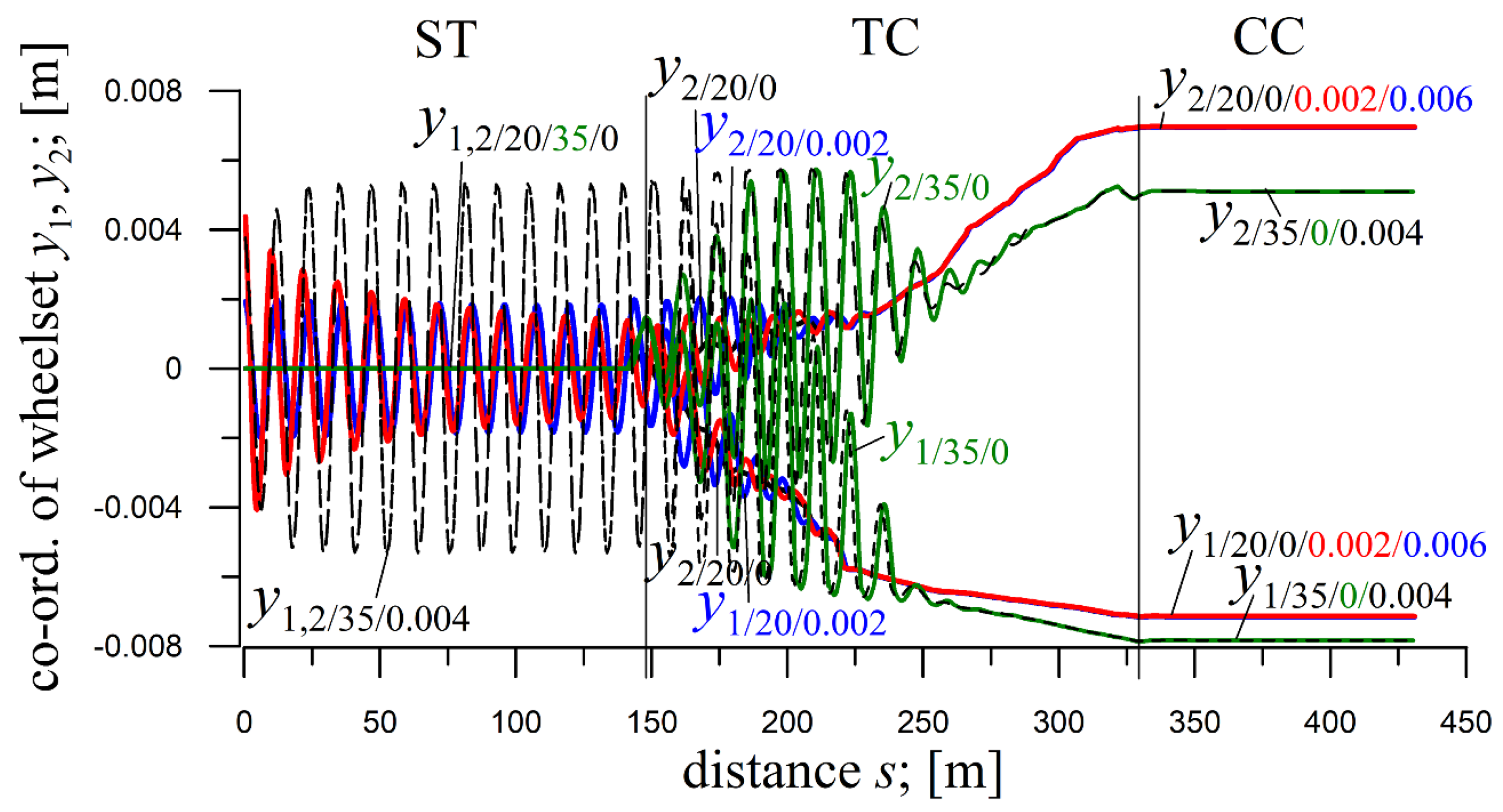
Figure 4.
Lateral displacements of front wheelsets in front and rear bogies of passenger car MKIII for R=2000 m; h=0.045 m; ST (l=300 m), TC (l=180.46 m), CC (l=500 m); v=20 m/s at yj(0)=0, 0.002, and 0.006 m.
Figure 4.
Lateral displacements of front wheelsets in front and rear bogies of passenger car MKIII for R=2000 m; h=0.045 m; ST (l=300 m), TC (l=180.46 m), CC (l=500 m); v=20 m/s at yj(0)=0, 0.002, and 0.006 m.
5. The Impact of Vehicle Velocity
5.1. The Bogie with Average Parameters
The influence of velocity v on solutions for the bogie with average parameters is presented in Figures 5a and 5b, obtained at E=0.01.
In Figure 5a, at v=30 and 34 m/s, vibrations in ST decay (approach stationary), indicating motion below vn in ST (actual vn values not determined). A limit cycle forms at v=36 m/s, indicating a stable periodic solution. Reducing the lateral stiffness kzy (0.4x multiple) lowers vn to below 36 m/s. Similar results occur in CC (at R=2000 m), with a limit cycle forming at v=36 m/s. Decreasing kzy lowers vn again (at nominal kzy and R=2000 m, vn=47.1 m/s [53]). The solutions in TC constitute a smooth transition from ST to CC for all mentioned v values.
In Figure 5b at v=60 m/s (and not illustrated v<60 m/s), vibrations in ST decay (approach stationary) and become stationary in CC. So, the motion in ST and CC of R=2000 m occurs below the respective vn. The solutions in TC constitute a smooth transition from the solutions in ST to those in CC.
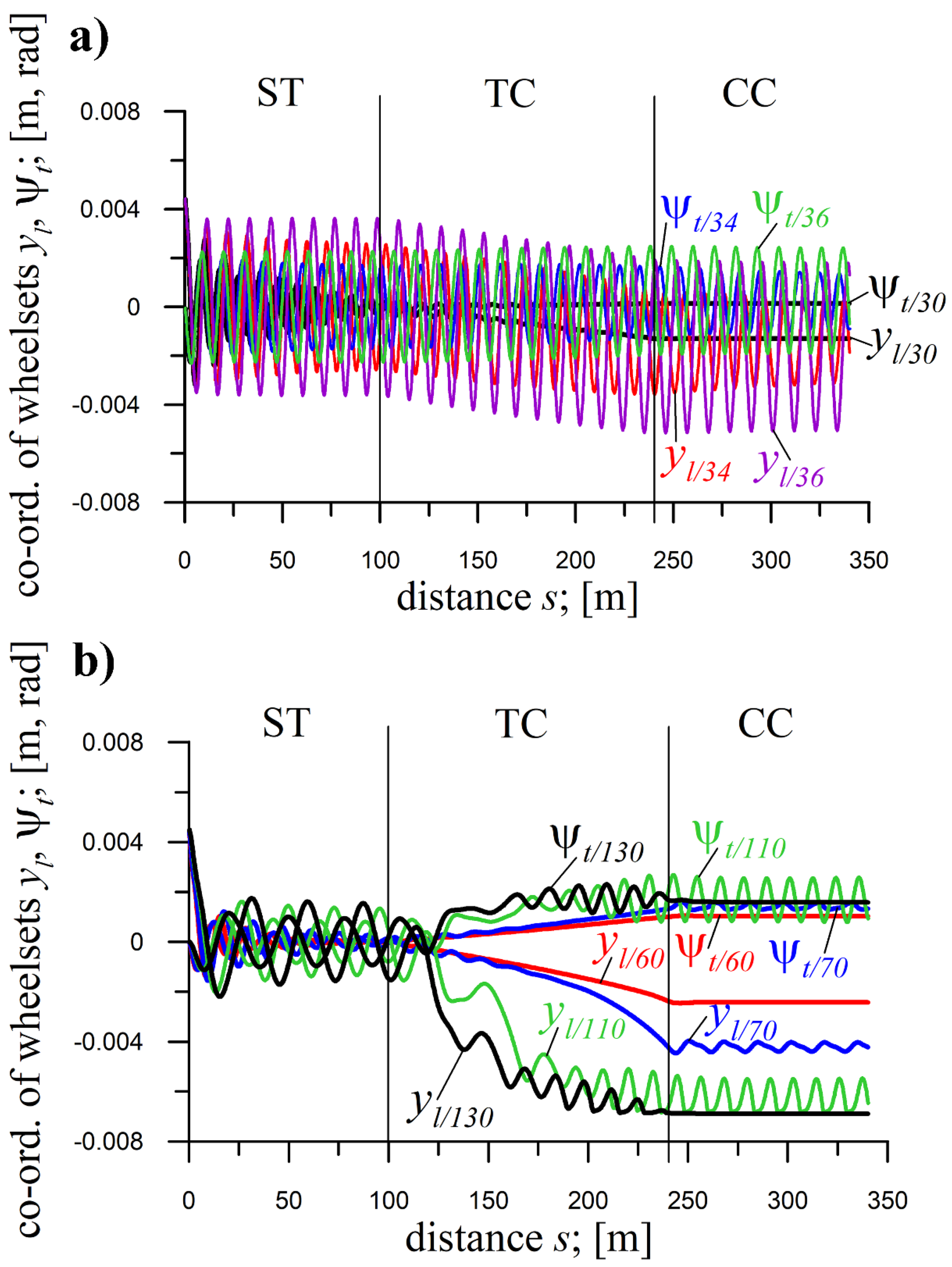
The results at v=70 m/s (Figure 5b) are still typical, but only for ST and TC. In ST, vibrations decay, while in TC, a smooth transition to CC exists. Periodic solutions in CC at v=70 m/s mean motion above vn (at R=2000 m). Decaying vibrations in ST at v=110 and 130 m/s, mean this vn is atypically much lower than in ST. 2-axle objects with nominal parameters (as in Table 1 and Table 2) show similar vn in ST and CCs [53]. In CC, at v=110 m/s, limit cycles still exist, although already initiated halfway through TC. Atypical change in solution type happens there, opposed to vibrations initiated only in the CC at v=70 m/s. In CC at v=130 m/s, solutions are stationary, thus atypical. Typically, solutions at higher v become periodic, whereas at the lower, they are stationary. In TC’s second half at v=130 m/s, solutions become atypical through specific vibrations that appear and then disappear at the TC’s end. The case of the bogie of MKIII car at R=300 m in Subsection 6.2 is similar.
Increasing kzx (40x multiple) leads to a significant rise in vn in ST and CC of R=2000 m (Figure 5b) to above 130 m/s and above 60 but below 70 m/s, respectively (at nominal kzx, the values are vn=45.8 and 41.7 m/s [53]). Unforeseenly, the 10x, 60x, 80x, and 100x multiples (not illustrated) result in solutions qualitatively and quantitatively similar to Figure 5b.
Figure 5.
Coordinates of wheelsets of the bogie with average parameters for R=2000 m; h=0.045 m; ST (l=100 m), TC (l=140 m), CC (l=100 m); yi(0)=0.0045 m at: a) kzy=1556 kN/m (0.4x) and v=30, 34, and 36 m/s, and b) kzx=104600 kN/m (40x) and v=60, 70, 110, and 130 m/s.
Figure 5.
Coordinates of wheelsets of the bogie with average parameters for R=2000 m; h=0.045 m; ST (l=100 m), TC (l=140 m), CC (l=100 m); yi(0)=0.0045 m at: a) kzy=1556 kN/m (0.4x) and v=30, 34, and 36 m/s, and b) kzx=104600 kN/m (40x) and v=60, 70, 110, and 130 m/s.
5.2. The Bogie of MKIII Passenger Car (Velocity)
The effect of v on the solutions for the bogie of MKIII passenger car is illustrated in Figures 6a and 6b, at E=0.4. Except for the v variants in these figures, v=10, 46, and 66 m/s were studied.
These results are systematised, but partly. In ST, they are for all v values. In CC, they are between v=10 and 46 m/s (Figure 6a). At v=54 m/s and larger (Figures 6a and 6b), nonlinear features manifest in unsystematised solutions along v increase.
In ST, at v=10, 36 and 41 m/s, decaying vibrations represent motion below vn for ST (v=36 m/s in Figure 6a). At v=46 m/s, a limit cycle establishes (Figure 6a), with motion above vn. It is also so at v=54, 62, 72 and 82 m/s (Figures 6a and 6b), with ST(l=100 m) too short to properly show it at v=54 and 62 m/s.
In CC, at v=10, 36 and 41 m/s (v=36 m/s in Figure 6a), the motion occurs below vn for CC of R=1200 m. At v=10 (not illustrated) and 36 m/s (Figure 6a), solutions are stationary, while at v=41 m/s (not illustrated), vibrations decay. At v=46 m/s, a limit cycle emerges in CC (Figure 6a), with motion above vn.
At v=54 m/s (Figure 6a), the solutions in CC remain periodic, with nonlinearities manifested through the loss of the symmetrical, quasi-harmonic character of displacements yl. Surprisingly, at v=62
Figure 6.
Coordinates of front and rear wheelsets of the bogie of MKIII passenger car for R=1200 m; h=0.075 m; ST (l=100 m), TC (l=140 m), CC (l=100 m); yi(0)=0.0045 m at: a) v=36, 46 and 54 m/s and b) v=62, 72, and 82 m/s m/s (Figure 6 b), the solutions in the CC approach a stationary (decaying vibrations). At v=66 m/s (not illustrated), the solutions become periodic again. However, losing the quasi-harmonic character of the yaw angle ψt reveals nonlinear features. At v=72 m/s (Figure 6b), the solutions are still periodic. However, the more distinct loss of quasi-harmonic character of yl and ψt exists. At v=82 m/s (Figure 6b), periodic solutions in CC continue, now with a much higher frequency than at smaller v. This frequency is also much higher than in ST and TC.
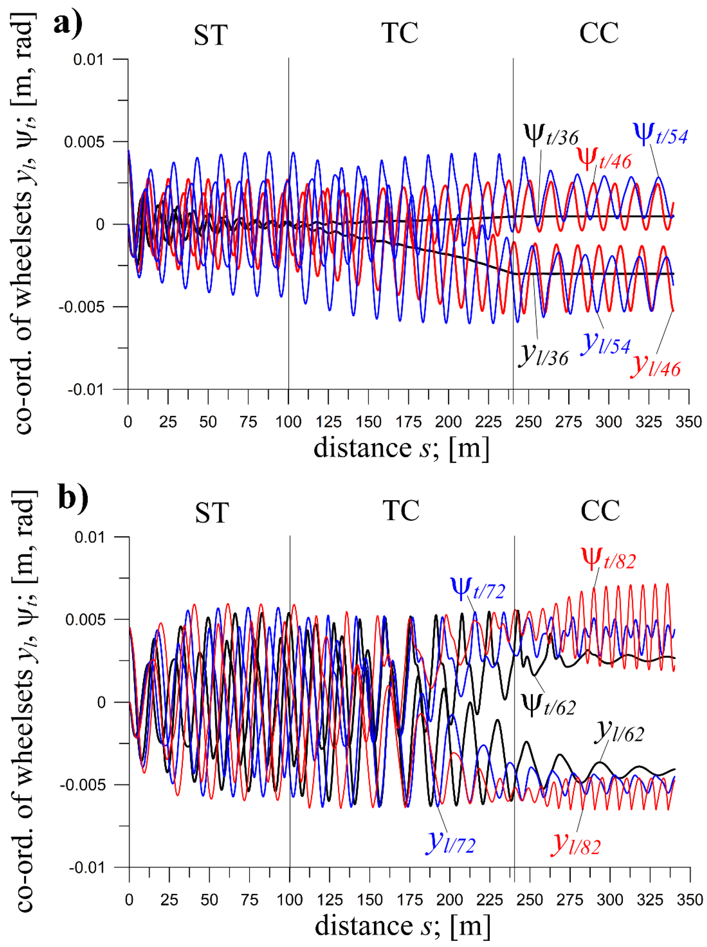
In TC, the transition from ST to CC is smooth. However, in TC’s second half, nonlinear features are noticeable at higher v=66, 72, and 82 m/s, preceding such features in CC (Figure 6b).
Nonlinear effects, particularly at higher velocities, presumably stem from the isolated bogie model lacking secondary suspension, relatively low mass, and base length, which amplify lateral displacements and make flange contact more probable.
5.3. The 2-Axle Empty Freight Car of Average Parameters (Velocity Impact)
The influence of v on solutions of the 2-axle empty freight car is shown in Figures 7a and 7b, at E=0.1. Except for R variants in these figures, the R=600 and 1200 m were tested.
These results are well systematised, showing typical behaviour around vn in ST and CC.
In ST, decaying vibrations or solutions approaching a stationary occur at v=20, 30, and 40 m/s, while limit cycles emerge at v=44 and 47 m/s, placing vn between 40 and 44 m/s.
In CC at R=450 m (Figure 7a), solutions remain stationary in the v range (20-45 m/s), indicating that the vn is higher than in ST. Besides, if the calculations were feasible, vn would be larger than the velocity vs of numerical derailment in CC of R=450 m (here vs>45 m/s).
At R=600 m (not illustrated), front wheelset displacements yl are stationary at v=30, 40, 44 and 47 m/s, while rear wheelset’s yt become periodic at v=44 and 47 m/s, marking vn as between 40 and 44 m/s, like in ST. This does not mean that vn in ST and CC at R=600 m are the same.
At R=1200 m (Figure 7b), stationary solutions at v=30 and 40 m/s exist, while periodic behaviour starts at v=44 m/s, again showing a similar range for vn (between 40-44 m/s). Again, it does not mean that the vn in ST and CCs at R=600 and 1200 m are identical.
At R=4000 m (not illustrated), responses qualitatively align with those at R=1200 m. Quantitatively, at R=4000 m, the amplitudes are larger, reduced asymmetry against the track centre line exists, similarity to the solutions in CC to those in ST appears, and the limit cycle at v=44 m/s starts from the CC’s very beginning.
Solutions in the TC transition smoothly from ST to CC, though at existing vibrations their behaviour varies by R. At R=450 m (Figure 7a), they disappear from the TC’s middle. At R=600 m (not illustrated), the yl vibrations (front wheelset) disappear at the TC’s end, while yt (rear wheelset) do not and continue in CC as a limit cycle. At R=1200 m and v=44 m/s (Figure 7b), the vibrations in TC’s end do not reach the amplitude as in CC. They do, at v=47 m/s (Figure 7b). At R=4000 m (not illustrated), the amplitudes in TC change insignificantly and have similar values as in ST and CC.
Figure 7.
Coordinate of leading wheelset of freight car of average parameters at ST (l=300 m), TC (l=102.4 m), CC (l=140 m); yi(0)=0.0045 m; and kzx=960 kN/m (1,2x); kzy=800 kN/m (1x); czx=71,4 kN⋅s/m (1,7x); czy=70,5 kN⋅s/m (1,5x): a) R=450 m; h=0.15m; v=20, 30, 40, 44 and 45 m/s, and b) R=1200 m; h=0.075 m; v=30, 40, 44 and 47 m/s.
5.4. The 2-Axle Loaded HSFV1 Freight Car (Velocity Impact)
The impact of v on solutions for the HSFV1 car is presented in Figure 8, at E=0.01. Except for v in Figure 8 (see figure caption), results for v=40, 45.3, and 48 m/s were studied.
The results in Figure 8 are naturally systematised.
In ST, stationary solutions or decaying vibrations occur at v=38, 40, and 42 m/s, while limit cycles occur at v=43 m/s and beyond, placing vn between 42 and 43 m/s (vn=42.8 m/s [53]).
In CC, solutions are stationary at v=38 m/s, while limit cycles start at v=40 m/s only for the front wheelset and with small amplitude, placing vn between 38 and 40 m/s (vn=40 m/s [53]). Starting from v=42 m/s, the limit cycle concerns both wheelsets, while amplitudes grow with v. They become considerable for v=43 and 49 m/s (also in ST). Small R=600 m in Figure 8 induces pronounced results asymmetry in CC compared to the symmetric ST responses.
In TC, the solutions transition smoothly from ST to CC in the entire v scope (between 38 and 49 m/s). From v=42 m/s, vibrations exist throughout TC, while from v=43 m/s, their amplitudes become significant.
Figure 8.
Coordinates of leading wheelset of HSFV1freight car; R=600 m; h=0.15 m; ST (l=150 m), TC (l=142 m), CC (l=150 m); yi(0)=0.0045 m; kzx=206,7 kN/m (0,1x) at v=38, 42, 43 and 49 m/s;.
Figure 8.
Coordinates of leading wheelset of HSFV1freight car; R=600 m; h=0.15 m; ST (l=150 m), TC (l=142 m), CC (l=150 m); yi(0)=0.0045 m; kzx=206,7 kN/m (0,1x) at v=38, 42, 43 and 49 m/s;.
5.5. The 4-Axle MKIII Passenger Car (Velocity Impact)
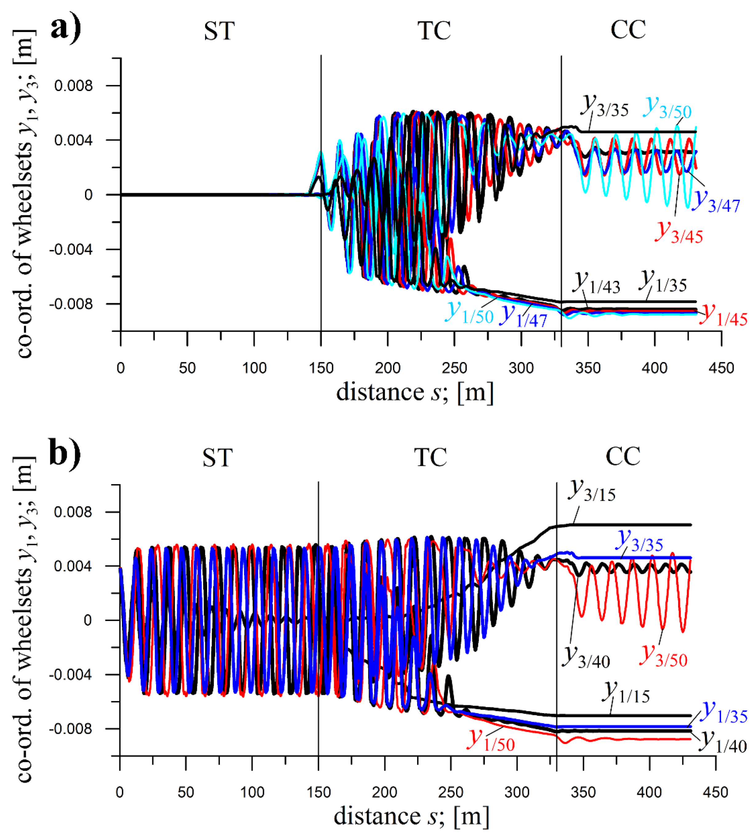
The impact of v on the solutions for the 4-axle MKIII car is shown in Figures 3 (Subsection 4.2), 9a, and 9b, at E=0.05. The impacts at zero (Figure 3 and Figure 9a) and non-zero (Figure 3 and Figure 9b) initial conditions yj(0) are considered.
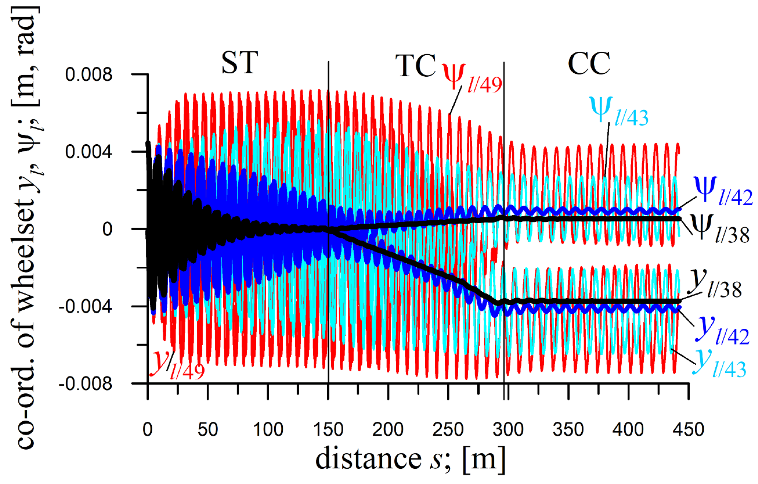
For yj(0)=0.0 m, solutions in ST are always stationary (Figure 3 and Figure 9a). For yj(0)=0.004 m, solutions shift from decaying (at v=15 m/s) to periodic (from v=20 to 50 m/s - Figure 3 and Figure 9b), setting vn between bordering values (vn=19.1 m/s [53]).
Results here confirm no influence of yj(0) applied in ST on solutions in CC (revealed in Section 4). So, solutions in CC at yj(0)=0.0 and 0.004 m are identical, and thus discussed jointly (see line pairs for different yj(0) at v=35 m/s in Figure 3 and at v=50 m/s in Figures 9a and 9b). In CC, solutions are stationary between v=15 and 35 m/s (Figures 3, 9a, and 9b), then between v=40 and 50 m/s become periodic (Figures 9a and 9b), but limited to the rear bogie (y3 coordinate). The y3 amplitudes are non-monotonic, varying irregularly with increasing v and highlighting strongly nonlinear features of the present vehicle. Specifically, they are greater at v=40 m/s than at v=43 m/s (Figure 9b); less at v=43 m/s (Figure 9b) than at v=45 m/s (Figure 9a); greater at v=45 m/s than at v=47 m/s (Figure 9a); and less at v=47 m/s than at v=50 m/s (Figures 9a and 9b).
In TC at yj(0)=0 m, and v=15 (not illustrated) and 20 m/s (Figure 3) vibrations resemble disturbances. At v=35 m/s and larger (Figure 3 and 9a), they become vibrations of high intensity. In TC at yj(0)=0.004 m and v=15 m/s (Figure 9b) solutions are identical as at yj(0)=0 m. At v=20 m/s and larger (Figures 3, 9a, and 9b), such identity (high similarity) only applies to the TC’s end, with vibration intensity rising with v growth. At any yj(0), the amplitudes are significantly bigger at the TC’s beginning than at its end.
Figure 9.
Lateral displacements of front wheelsets in front and rear bogies of passenger car MKIII; R=600 m; h=0,15 m; ST (l=150 m), TC (l=180.46 m), CC (l=100 m) for: a) yj(0)=0 m at v=35, 43, 45, 47 and 50 m/s and b) yj(0)=0.004 m at v=15, 35, 40 and 50 m/s.
Figure 9.
Lateral displacements of front wheelsets in front and rear bogies of passenger car MKIII; R=600 m; h=0,15 m; ST (l=150 m), TC (l=180.46 m), CC (l=100 m) for: a) yj(0)=0 m at v=35, 43, 45, 47 and 50 m/s and b) yj(0)=0.004 m at v=15, 35, 40 and 50 m/s.
6. The Impact of the Curve Radius
6.1. The 25TN Freight Car Bogie
The effect of radius R on the solutions for the 25TN bogie is represented in Figures 10a, 10b, and 2 (Subsection 4.1), at E=0.01. It is discussed by comparing R=300 and 900 m cases, but at individual v. It expands the study on the impact of v in Section 5.
In Figure 10a, for v=10 m/s, solutions in ST occur below the critical velocity vn, showing decaying vibrations. In CC at R=300 m, solutions are stationary, whereas at R=900 m, low-amplitude vibrations decay to a stationary state. In TC, slight vibrations disappear smoothly towards TC’s end. In CC and TC, front wheelset displacements yl are larger for R=300 m than R=900 m. Negative yl indicates the curve turns leftward, and the displacement is towards the curve’s outside.
In Figure 10a, as v increases to 14 m/s, the motion in ST is above vn (periodic vibrations). In CC at R=300 m, yl are stationary, while yt of the rear wheelset (not illustrated) are periodic, with very low amplitude. At R=900 m, yl and yt are periodic. In TC, solutions make smooth transitions to CCs, with vibrations decreasing for both R.
The v=12 m/s, also tested (not illustrated), appeared qualitatively the same as at v=14 m/s, but of lower amplitudes.
In Figure 10b, solutions (yl and not illustrated yt) in ST possess a similar nature at v=29.5, 35, and 38.5 m/s, and so do those in TCs. In ST, the solutions occur below vn. However, the higher v, the longer the initial vibrations disappear. In TCs, the solutions form a vibration-free smooth passage to CCs, for both R, with disturbances during the ST-TC and TC-CC transitions.
Figure 10.
Coordinates of front wheelsets of 25TN bogie of a freight car for ST (l=86.5 m), TC (l=95 m), CC (l=98 m); yi(0)=0.0045 m, R=300 m and h=0,15 m and R=900 m and h=0,142 m for a) kzy=389 kN/m (0.1x) at v=10 and 14 m/s and b) kzy=7780 kN/m (2x) at v=29.5, 35 and 38.5 m/s.
Figure 10.
Coordinates of front wheelsets of 25TN bogie of a freight car for ST (l=86.5 m), TC (l=95 m), CC (l=98 m); yi(0)=0.0045 m, R=300 m and h=0,15 m and R=900 m and h=0,142 m for a) kzy=389 kN/m (0.1x) at v=10 and 14 m/s and b) kzy=7780 kN/m (2x) at v=29.5, 35 and 38.5 m/s.
In Figure 10b, solutions (yl and not illustrated yt) in CC differ depending on v and R. At v=29.5 m/s, they are periodic (of low amplitude) at R=300 m and stationary at R=900 m. At v=35 m/s, they become stationary after some time at R=300 and 900 m; however, at a lower frequency for R=900 m. At v=38.5 m/s, they are periodic at R=300 and 900 m; however, for R=900 m, they have a lower frequency and longer time to establish (exceeding the CC’s length, l=98 m). Such unordered behaviours in CC disclose strong nonlinearities..
In Figure 10 b for CC and TC, at any v, the displacements towards the curve’s outside are larger at R=300 than at R=900 m, except yl, at v=38.5 m/s, in the TC’s second half, smaller.
Besides, the lowered kzy (0.1x – Figure 10a) decreased vn compared to the nominal kzy (Figure 2). Judging by Figure 10a, vn are between 10 and 12 m/s for ST, and CCs with R=300, and 900 m, while in [53], corresponding vn at nominal kzy equal 29.2, 29.1 and 29.2 m/s, respectively. The raised kzy (2x – Figure 10b) increased vn in ST and CC at R=900 m, compared to the nominal kzy (Figure 2). For R=300 m, vn seems close to that for the nominal kzy. Judging by Figure 10b, vn in ST is larger than 38.5 m/s, while in CC at R=900 m is between 35 and 38.5 m/s, which are higher than values from [53].
6.2. The MKIII Passenger Car Bogie (Curve Radius)
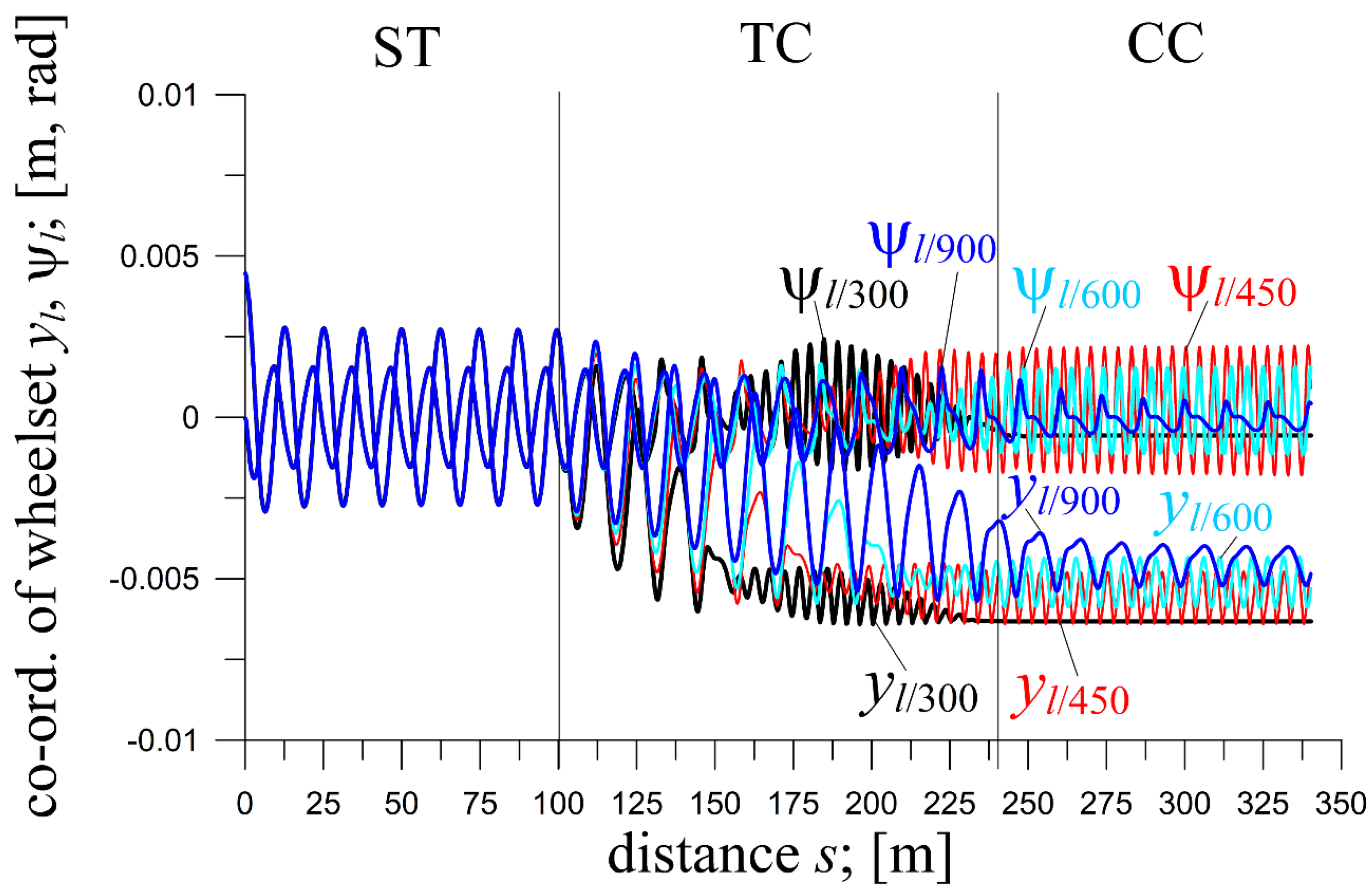
The impact of R on the bogie of MKIII passenger car is illustrated in Figure 11 and Figure 6a (Subsection 5.2), at E=0.4.
In ST, the motion is typical for v above vn, represented by limit cycles.
Contrarily, the results for TC and CC are atypical, due to strong nonlinearities.
The result in TC at R=300 m (Figure 11) is atypical. At about 2/5 of TC’s length, a change happens in the nature of vibrations, switching from lower to higher frequency, while at TC’s end, vibrations disappear. Such a phenomenon was identified, and the origin explained, in [35]. It reflects solutions the system takes in CC for R range that corresponds to the radii the TC in Figure 11 (for the CC of R=300 m) possesses in its middle part (here R between 450 and 700 m). In Figure 11, in CCs for R=450 and 600 m, periodic solutions of frequency and amplitudes identical to those in the TC for R=300 m can be seen.
The solutions in TCs at R=450 and 600 m (Figure 11) feature similar frequency switches as at R=300 m. They appear slightly behind 1/2 and about 3/4 of the TC's length. Differently, the vibrations do not disappear but increase at the TC’s end and continue in CC.
It is different in TCs at R=900 and 1200 m (Figure 11 and Figure 6a – v=46 m/s); smooth transitions from ST to CC happen. Vibration frequencies in ST, TCs, and CCs remain similar. Different are the amplitudes, larger at R=1200 m.
In CC, at R=300 m, the solution is stationary (motion below vn in CC at R=300 m), whereas at R=450 and 600 m the solutions are periodic (limit cycles – motion above vn in CCs at R=450 and 600 m); Figure 11. Atypical for R=450 and 600 m are the frequencies in CCs much higher than in ST. However, the amplitudes are somewhat lower at R=600 m. The results in CCs at R=900 and 1200 m (Figure 11 and Figure 6a – v=46 m/s) are periodic with frequencies close to that in ST, and the amplitudes are considerably lower. Regular quasi-harmonic picture of the solutions is spoiled at R=900 m, while at R=1200 m this is preserved.
Figure 11.
Coordinates of front wheelset of bogie of MKIII passenger car for v=46 m/s; ST (l=100 m), TC (l=140 m), CC (l=100 m); yi(0)=0.0045 m at R=300, 450 and 600 m; h=0.15 m, and R=900 m; h=0.1 m.
Figure 11.
Coordinates of front wheelset of bogie of MKIII passenger car for v=46 m/s; ST (l=100 m), TC (l=140 m), CC (l=100 m); yi(0)=0.0045 m at R=300, 450 and 600 m; h=0.15 m, and R=900 m; h=0.1 m.
6.3. The 2-Axle Loaded HSFV1 Freight Car (Curve Radius)
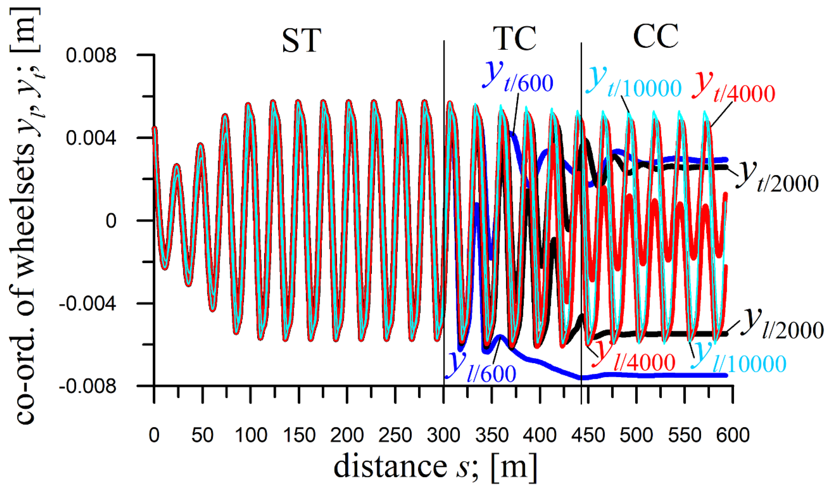
The R influence on the HSFV1 freight car is presented in Figure 12, at E=0.01. Except for longitudinal stiffness kzx in Figure 12, the nominal (Table 1) and reduced (206.7 kN/m – 0.1x) values were tested.
All these results are naturally systematised.
In Figure 12, for adopted v=45.3 m/s, solutions are periodic in ST and CCs at R=10000 and 4000 m (limit cycles – v>vn). The solutions are stationary (v<vn) in CCs of R=600 and 2000 m. The vibrations disappear in TC for R=600 m, while in CC at R=2000 m. At R=4000 m, the amplitudes in CC are smaller than in ST, while at R=1000 m, they are almost the same. Also, at R=4000 m, considerable solutions asymmetry against the track centre line exists, while at R=1000 m it is virtually invisible. Despite such different solutions in CCs, the solutions in TC make smooth transitions from the ST to CC.
For the 0.1x multiple and the nominal kzx, v=45.3 m/s proves higher than vn for CCs at any R and ST (limit cycle solutions). However, the smaller R, the smaller amplitudes, and the more considerable asymmetry of solutions against the track centre line in CCs. The bigger the R, the closer the amplitude values in CC and ST. In TC, the transition of solutions from the ST to CC is smooth for all tested R.
Confronting results for the 0.1x and 20x multiples shows that bigger kzx increases vn in CCs of medium R=600 and 2000 m and decreases vibration frequencies in ST, TC and CC at the same v.
Figure 12.
Lateral displacements of front and rear wheelsets of HSFV1freight car for v=45.3 m/s; ST (l=300 m), TC (l=142 m), CC (l=150 m); yi(0)=0.0045; kzx=41340 kN/m (20x) at R=600, 2000, 4000 and 10000 m and h=0.15, 0.045, 0.0225 and 0.009 m, respectively .
Figure 12.
Lateral displacements of front and rear wheelsets of HSFV1freight car for v=45.3 m/s; ST (l=300 m), TC (l=142 m), CC (l=150 m); yi(0)=0.0045; kzx=41340 kN/m (20x) at R=600, 2000, 4000 and 10000 m and h=0.15, 0.045, 0.0225 and 0.009 m, respectively .
7. Conclusions
7.1. The Detailed Conclusions
The significant results identified in the course of the presented study are:
The study reveals several important results related to the influence of initial conditions, velocity, and curve radius on the dynamic behaviour of different vehicle bogies, freight cars, and passenger car:
- Impact of initial conditions yj(0) and yi(0):
- For the 25TN freight car bogie, identical periodic solutions were found in CC for all initial conditions yj(0) (imposed in ST) at medium (R=900 m) and moderate (R=2000 m) radii. Sameness of vibration-free solutions in the final part of TC at R=900 m for all yj(0).
- For the MKIII passenger car bogie, periodic solutions in CC at small radius (R=600 m) and solutions, with increasing vibrations, in the TC’s final part (at that R) were disclosed as identical for all yi(0).
- The 4-axle MKIII passenger car showed in CC identical stationary solutions at small and medium radii (R=600 and 1200 m) and periodic at moderate R=2000 m for all yi(0). Sameness of vibration-free solutions in the TC’s final part (at R=600 m) for all yj(0). Besides, multiple solutions were observed [35] in ST for different yi(0) with their no-effect for solutions identity in CC at R=600, 1200, and 2000 m. Multiple solutions in CC existed at larger radii (R=4000, 6000, 10000 m).
- Impact of velocity v:
- For the bogie with average parameters, a systematic increase in v showed a gradual shift from stationary solutions to periodic (limit cycles) once v exceeded the critical velocity vn. In ST, at v<vn, a higher length was needed for vibration to fade, and in ST and CC, at v≥vn, the periodic solutions’ amplitude increased with v increases. In TC, at all v, a smooth passage from ST to CC existed. This systematised image experienced an exception in CC at R=2000 m and v=130 m/s, where solutions returned from periodic to stationary.
- The bogie of MKIII passenger car exhibited systematised solutions for ST, TC, and CC at smaller v. At v>vn, solutions’ unpredictability occurred in CC at R=1200 m (and R=900 m [35]) and v between 54 and 82 m/s.
- The 2-axle freight car of average parameters showed generally typical solutions, except at R=600 m, where front and rear wheelsets' solutions differ (stationary vs. periodic).
- The 2-axle HSFV1 freight car showed the systematised solutions for all R at any v.
- The 4-axle MKIII passenger car showed systematised solutions for ST, TC, and CC at smaller v. At v>vn in CC, solutions unpredictability occurred at R=600 m and v between 43 and 50 m/s.
- Impact of curve radius R:
- For the 25TN bogie, a typical solution pattern emerged with increasing R. At low velocities v, stationary solutions existed in ST and CC for all R. As v increased, periodic solutions emerged in ST and CC at higher radii. At the highest v, periodic solutions appeared in both ST and CC. At smaller R=300 to 900 m, atypical behaviours were observed, such as disappearing vibrations in TC (despite their existence in ST and CC) and switching between periodic and stationary solutions (and vice versa) in CC [35].
- For the bogie of MKIII passenger car, solutions are partially typical as R increases. Atypical higher vibration amplitudes in CC and single or multiple changes of solution type in TC occurred at smaller R.
- The 2-axle freight car showed a partly systematised picture of solutions for increasing R. Atypical behaviours included different solution types for front and rear wheelsets at R=600 m (and R=900 and 1200 m [35]).
- The 2-axle hsfv1 freight car displayed typical behaviour for increasing R at many suspension configurations (for the selected one, at R between 450 and 650 m, limit cycles occurred in CC, despite their absence in ST and no vibrations in TC (to be discussed in the planned following paper)).
7.2. The Very General Conclusions
From the systematic motion conditions’ variants, the study provides the following general conclusions:
- Initial conditions in ST did not affect the solutions in CC, except in cases where multiple solutions existed in ST and/or CC.
- A mostly systematised solutions pattern exists in ST, TC, and CC for increasing velocity, except for results unpredictability in CCs only, facilitated by high speeds.
- The solutions for gradually increasing curve radius showed a mostly systematic pattern. Its perturbations mainly concern small and medium R (300 to 1200 m). For the 4-axle vehicle, the perturbing multiple solutions also appear in CCs of moderate and large radii.
Author Contributions
Conceptualisation, K.Z.; methodology, K.Z.; software, K.Z.; validation, KZ. and M.G.-S.; formal analysis, K.Z.; investigation, M.G.-S., and K.Z.; resources, M.G.-S.; data curation, K.Z.; writing—original draft preparation, M.G.-S. and K.Z.; writing—review and editing, K.Z.; visualisation, M.G.-S.; supervision, K.Z.; project administration, K.Z.; funding acquisition, M.G.-S. and K.Z. All authors have read and agreed to the published version of the manuscript.
Funding
This work is a result of the research project financed by the National Science Centre, Poland, under the project no. 2014/15/N/ST8/02668.
Data Availability Statement
The original contributions presented in the study are included in the article; further inquiries can be directed to the corresponding author.
Conflicts of Interest
The authors declare no conflicts of interest.
References
- Hoffmann, M. Dynamics of European two-axle freight wagons. Ph.D. thesis, Technical University of Denmark, Informatics and Mathematical Modelling, Lyngby, 2006.
- Hoffmann, M.; True, H. The dynamics of two-axle freight wagons with UIC standard suspension, Proc. of the 10th VSDIA Conference, Budapest University of Technology and Economics, 2006, pp. 183-190. ISBN 978-963-420-968-3.
- Wang, K.; Liu, P. Lateral stability Analysis of Heavy-Haul Vehicle on Curved Track Based on Wheel/Rail Coupled Dynamics. Journal of Transportation Technologies 2, 150-157, 2012.
- Dusza, M. The study of track gauge influence on lateral stability of 4-axle rail vehicle model, Archives of Transport, 30(2), 7-20, 2014.
- Zboinski, K. Dynamical investigation of railway vehicles on a curved track, Eur. J. Mech. A-Solids 17(6), 1001-1020, 1998.
- Zboinski, K.; Golofit-Stawinska, M. Non-linear dynamics of railway vehicles in transition curves around critical velocity with focus on 2-axle cars, in M. Spiryagin, et al. (eds.),The Dynamics of Vehicles on Roads and Tracks – Proc. 24th IAVSD Symp., Rockhampton, Queensland, Australia, 2018, CRC Press, pp. 599-604. ISBN: 978-1-138-48263-0.
- Zboinski, K.; Golofit-Stawinska, M. 2018. [CrossRef]
- Zhai, W. M.; Wang, K.Y. s: interactions of trains and tracks on small radius curves, 2006. [CrossRef]
- Kurzeck, B.; Hecht, M. 2010. [CrossRef]
- Kondo, O.; Yamazaki, Y. Simulation Technology for Railway Vehicle Dynamics, Nippon Steel & Sumitomo Metal Technical Report No. 105 (December), 77-83, 2013.
- Prandi, D. Railway Bogie Stability Control From Secondary Yaw Actuators, M.Sc. thesis, Politecnico di Milano, Scuola di Ingegneria Industriale e dell'Informazione, 2014.
- Matsumoto, A.; Michitsuji, Y. Analysis of Flange-Climb Derailments of Freight Trains on Curved Tracks Due to Rolling, Proc. 10th International Conference on Railway Bogies and Running Gears, Scient. Soc. of Mech. Engineers, Budapest, pp. 91-100, 2016, ISBN 978-963-9058-38-5.
- Shaltout, R.; Baeza, L.; Ulianov, C. Development of a simulation tool for the dynamic analysis of railway vehicle-track interaction, Transp. Probl. 2015; 10. [Google Scholar] [CrossRef]
- Lau, A.; Kassa, E. Simulation of Vehicle-Track Interaction in Small Radius Curves and Switches and Crossings, in J. Pombo (ed.), Proc. of the Third Intl. Conf. on Railway Technology: Research, Development and Maintenance. Stirlingshire, UK. 2016. [Google Scholar] [CrossRef]
- Kufver, B. Optimisation of Horizontal Alignments for Railway – Procedure Involving Evaluation of Dynamic Vehicle Response. Ph.D. thesis, Royal Institute of Technology, Stockholm, 2000.
- Long, X.Y.; Wei, Q.C.; Zheng, F.Y. : Dynamical analysis of railway transition curves. Proc. IMechE part F Journal of Rail and Rapid Transit, 224(1), 1-14, 2010.
- Zboinski, K.; Woznica, P. Combined use of dynamical simulation and optimisation to form railway transition curves, Vehicle Syst. Dyn., 56(9), 1394- 1450, 2018. [Google Scholar] [CrossRef]
- Huilgol, R.R. . Hopf-Friedrichs bifurcation and the hunting of a railway axle. Quart. J. of Appl. Math. 36, 85-94, 1978.
- Gasch, R.; Moelle, D.; Knothe, K. The effect of non-linearities on the limit-cycles of railway vehicles, in: Hedrick, K. (ed.), Proc. 8th IAVSD Symposium, Cambridge, USA. Swets & Zeitlinger, Lisse, pp. 207-224, 1984.
- True, H.; Hansen, T.G.; Lundell, H. On the Quasi-Stationary Curving Dynamics of a Railroad Truck, Proc. ASME/IEEE/AREA Joint Railroad Conference, ASME-RTD 29, pp. 131-138, 2005.
- True, H. Recent advances in the fundamental understanding of railway vehicle dynamics, Int. J. Vehicle Des. 40(1/2/3), 251-264, 2006.
- Polach, O. Characteristic parameters of nonlinear wheel/rail contact geometry, Vehicle Syst. Dyn. 48(suppl.), 19-36, 2010.
- True, H. Multiple attractors and critical parameters and how to find them numerically: the right, the wrong and the gambling way, Vehicle System Dynamics, 51(3), 443-459, 2013. [CrossRef]
- Di Gialleonardo, E.; Bruni, S.; True, H. Analysis of the non-linear dynamics of a 2-axle freight wagon in curves. Vehicle Syst. Dyn. 2014. [Google Scholar] [CrossRef]
- Zboinski, K.; Dusza, M. Extended study of rail vehicle lateral stability in a curved track, Vehicle System Dynamics 49(5), 789-810, 2011.
- Zboinski, K.; Dusza, M. 2017. [CrossRef]
- Zboinski, K. Modelling dynamics of certain class of discrete multi-body systems based on direct method of the dynamics of relative motion. Meccanica 47(6), 1527- 1551, 2012, Springer, . [Google Scholar] [CrossRef]
- Kuba, T. ; Lugner. P. 2012. [Google Scholar] [CrossRef]
- Carballeira, J.; Baeza, L.; Rovira, A.; García, E. Technical characteristics and dynamic modelling of Talgo trains, Veh. Syst. 2008. [Google Scholar] [CrossRef]
- Lurie, A.I. Analytical Mechanics, Springer-Verlag, 1st ed. Berlin, Heidelberg, New York, 2002, 864 p. (originally: Lurie A.I., Analiticeskaja mechanika, FizMatGIZ, Moscow 1961. Russian).
- Kik, W. Comparison of the behaviour of different wheelset-track models, in: Sauvage, G. (ed.), Proc. 12th IAVSD Symp. on The Dynamics of Vehicles on Roads and on Tracks. Vehicle Syst.Dyn. 20(suppl.), 325-339, 1992.
- Kalker, J.J. A fast algorithm for the simplified theory of rolling contact. Vehicle Syst. Dyn. 11, 1-13, 1982.
- Hairer, E.; Wanner, G. Solving Ordinary Differential Equations, part II: Stiff and differential-algebraic problems, Springer, 1991.
- Xu, G.; Steindl, A.; Troger, H. Nonlinear stability analysis of a bogie of a low-platform wagon. Proc. 12th IAVSD Symp. on The Dynamics of Vehicles on Roads and on Tracks, Vehicle Syst. Dyn. 20(suppl.), 653-665, 1992.
- Zboinski, K.; Golofit-Stawinska, M. Investigation into nonlinear phenomena for various railway vehicles in transition curves at velocities close to critical one. Nonlinear Dynamics, 98(3), 1555- 1601, 2019. [Google Scholar] [CrossRef]
- Bustos, A.; Tomas-Rodriguez, M.; Rubio, H.; Castejon, C. On the nonlinear hunting stability of a high-speed train boogie, Nonlinear Dynamics 2023, 111, 2059–2078. [CrossRef]
- Ge, P.; Wie, X.; Liu, J.; Cao, H. Bifurcation of a modified railway wheelset model with nonlinear equivalent conicity and wheel–rail force, Nonlinear Dynamics 2020, 102, 79–100. [CrossRef]
- Guo, J.; Shi, H.; Luo, R.; Zeng, J. Bifurcation analysis of a railway wheelset with nonlinear wheel–rail contact, Nonlinear Dynamics 2021, 104, 989–1005. [CrossRef]
- Guo, J.; Zhang, G.; Shi, H.; Zeng, J. Small amplitude bogie hunting identification method for high-speed trains based on machine learning, Vehicle System Dynamics, Published online 19 Jun 2023. https://doi.org /10.1080/00423114.2023.2224906.
- Pandey, M.; Bhattacharya, B. Effect of bolster suspension parameters of three-piece freight bogie on the lateral frame force, International Journal of Rail Transportation 2020, 8(1), 45-65. [CrossRef]
- Skerman, D.; Colin Cole, C.; Spiryagin, M. Determining the critical speed for hunting of three-piece freight bogies: practice versus simulation approaches, Vehicle System Dynamics 2022, 60(10), 3314-3335. [CrossRef]
- Sun, J.; Chi, M.; Jin, X.; Liang, S.; Wang, J.; Li, W. Experimental and numerical study on carbody hunting of electric locomotive induced by low wheel–rail contact conicity, Vehicle System Dynamics 2021, 59(2), 203-223. https://doi.org /10.1080/00423114.2019.1674344.
- Sun, J.; Meli, E.; Song, X.; Chi, M.; Jiao, W.; Jiang, Y. A novel measuring system for high-speed railway vehicles hunting monitoring able to predict wheelset motion and wheel/rail contact characteristics, Vehicle System Dynamics 2023, 61(6), 1621-1643. [CrossRef]
- Umemoto, J.; Yabuno, H. Parametric and self-excited oscillation produced in railway wheelset due to mass imbalance and large wheel tread angle, Nonlinear Dynamics 2023, 111:4087–4106. [CrossRef]
- Wang, X.; Lu, Z.; Wen, J.; Wie, J.; Wang, Z. Kinematics modelling and numerical investigation on the hunting oscillation of wheel-rail nonlinear geometric contact system, Nonlinear Dynamics 2022, 107: 2075–2097. [CrossRef]
- Yang, C.; Huang, Y.; Li, F. Influence of Curve Geometric Parameters on Dynamic Interactions of Side-Frame Cross-Braced Bogie. Proceedings ICRT 2021, Second International Conference on Rail Transportation, 2022. [Google Scholar]
- Liang, J.; Sun, J.; Jiang, Y.; Pan, W.; Jiao, W. Advances and Challenges in the Hunting Instability Diagnosis of High-Speed Trains. Sensors 2024, 24, 5719. [Google Scholar] [CrossRef] [PubMed]
- Bhardawaj, S.; Sharma, R.C.; Sharma, S.K. Development in the modeling of rail vehicle system for the analysis of lateral stability. Materials Today: Proceedings 2020, 25, 610–619. [Google Scholar] [CrossRef]
- Brustad, T.F.; Dalmo, R. Railway Transition Curves: a Review of the State-of-the-Art and Future Research. Infrastructures 2020, 5, 43. [Google Scholar] [CrossRef]
- Sadeghi, J.; Rabiee, S.; Felekari1, P. , Khajehdezfuly A. Investigation on optimum lengths of railway clothoid transition curves based on passenger ride comfort. Proceedings of the Institution of Mechanical Engineers, Part F: Journal of Rail and Rapid Transit. [CrossRef]
- Koc, W. New Transition Curve Adapted to Railway Operational Requirements. Journal of Surveying Engineering. [CrossRef]
- Kobryń, A. Design of curvilinear sections in vertical alignment of roads and railways using general transition curves. Automation in Construction 2024, 163, 105423. [Google Scholar] [CrossRef]
- Zboinski, K.; Golofit-Stawinska, M. Determination and Comparative Analysis of Critical Velocity for Five Objects of Railway Vehicle Class. Sustainability 2022, 14, 6649. [Google Scholar] [CrossRef]
- Zboinski, K.; Golofit-Stawinska, M. Dynamics of a Rail Vehicle in a Transition Curve above the Critical Velocity with a Focus on Hunting Motion Considering a Review of the History of Stability Studies. Energies 2024, 17, 967. [Google Scholar] [CrossRef]

Table 1.
Parameters of models for the adopted 2-axle objects.
|
Nota-tion |
Description |
Unit |
Parameter value | ||||
| 25TN bogie | Bogie aver. param. | Bogie MKIII car | Freight car av. param. | HSFV1 freight car | |||
 |
vehicle body/bogie frame mass | kg | 1 600 | 1 600 | 2 707 | 10 000 | 30 000 |
| m | wheelset mass | kg | 1 400 | 1 400 | 1 375 | 2 400 | 2 392 |
 |
vehicle body/bogie frame moment of inertia; longitudinal axis | kgm2 | 790 | 790 | 1 800 | 5 830 | 51 000 |
 |
vehicle body /bogie frame moment of inertia; lateral axis | kgm2 | 1 000 | 1 000 | 3 500 | 61 700 | 240 000 |
 |
vehicle body /bogie frame moment of inertia; vertical axis | kgm2 | 1 090 | 1 090 | 3 500 | 61700 | 222 000 |
 |
wheelset moment of inertia; longitudinal axis | kgm2 | 747 | 747 | 790 | 1 700 | 1 662 |
 |
wheelset moment of inertia; lateral axis |
kgm2 | 131 | 131 | 100 | 200 | 50 |
 |
wheelset moment of inertia; vertical axis |
kgm2 | 747 | 747 | 790 | 1 700 | 1 662 |
 |
longitudinal stiffness of the primary suspension | kN/m | - | 2 615 | 880 | 800 | 2 067 |
| kzy | lateral stiffness of the primary suspension |
kN/m | 3 890 | 3 890 | 3 925 | 800 | 431 |
 |
vertical stiffness of the primary suspension | kN/m | 1 017 | 1 017 | 2 667 | 1 000 | 4 100 |
 |
longitudinal damping of the primary suspension | kNs/m | - | 52.2 | 0 | 42 | 0 |
| czy | lateral damping of the primary suspension | kNs/m | 42 | 42 | 0 | 47 | 56 |
 |
vertical damping of the primary suspension | kNs/m | 7 | 7 | 170 | 60 | 28 |
| a | semi-wheel base | m | 0.9 | 0.9 | 1.3 | 3.16 | 3.15 |
| hb | vertical distance wheelset and vehicle body/bogie frame mass centres | m | 0.25 | 0.25 | 0.303 | 1.04 | 1.175 |
 |
wheelset rolling radius | m | 0.46 | 0.46 | 0.457 | 0.46 | 0.375 |
Table 2.
Parameters of the model of 4-axle passenger (car except its bogie) and models of track.
| Notation | Description | Unit | Parameter value |
| mp | vehicle body mass | kg | 28 658 |
| Iξp | body moment of inertia; longitudinal axis | kg⋅m2 | 35 986 |
| Iηp | body moment of inertia; lateral axis | kg⋅m2 | 1 089 000 |
| Iζp | body moment of inertia; vertical axis | kg⋅m2 | 1 089 000 |
| kpx | longitudinal stiffness of the secondary suspension | kN/m | 20 |
| kpy | lateral stiffness of the secondary suspension | kN/m | 476 |
| kpz | vertical stiffness of the secondary suspension | kN/m | 828 |
| kpφ | bogie frame-car body secondary roll stiffness | kN⋅m/rad | 1 822 |
| cpx | longitudinal damping of secondary suspension | kN⋅s/m | 0.5 |
| cpy | lateral damping of secondary suspension | kN⋅s/m | 80 |
| cpz | vertical damping of secondary suspension | kN⋅s/m | 53 |
| ap | half of bogies pivot distance | m | 8 |
| hp | vertical distance between bogie frame and car body mass centres | m | 1.343 |
| mt | vertical mass of the rail | kg | 200 |
| kt | vertical stiffness of the rail | kN/m | 70 000 |
| ct | vertical damping of the rail | kNs/m | 200 |
| mty | lateral mass of the track | kg | 500 |
| kty | lateral stiffness of the track | kN/m | 25 000 |
| cty | lateral damping of the track | kNs/m | 500 |
Disclaimer/Publisher’s Note: The statements, opinions and data contained in all publications are solely those of the individual author(s) and contributor(s) and not of MDPI and/or the editor(s). MDPI and/or the editor(s) disclaim responsibility for any injury to people or property resulting from any ideas, methods, instructions or products referred to in the content. |
© 2025 by the authors. Licensee MDPI, Basel, Switzerland. This article is an open access article distributed under the terms and conditions of the Creative Commons Attribution (CC BY) license (http://creativecommons.org/licenses/by/4.0/).
Copyright: This open access article is published under a Creative Commons CC BY 4.0 license, which permit the free download, distribution, and reuse, provided that the author and preprint are cited in any reuse.


