
Submitted:
21 October 2025
Posted:
23 October 2025
You are already at the latest version
Abstract
Objective: Predicting driver fatigue states is crucial for traffic safety. This study develops a deep learning model based on electroencephalogaphy (EEG) signals and multi-time-step historical data to predict the next time-step fatigue indicator percentage of eyelid closure (PERCLOS), while exploring the impact of different EEG features on prediction performance. Approach: A CTL-ResFNet model integrating CNN, Transformer Encoder, LSTM, and residual connections is proposed. Its effectiveness is validated through two experimental paradigms: Leave-One-Out Cross-Validation (LOOCV) and pretraining-finetuning, with comparisons against baseline models. Additionally, the performance of four EEG features differential entropy, α/β band power ratio, wavelet entropy, and Hurst exponent—is evaluated, using RMSE and MAE as metrics. Main Results: The combined input of EEG and PERCLOS significantly outperforms using PERCLOS alone validated by LSTM, CTL-ResFNet surpasses baseline models under both experimental paradigms, In LOOCV experiments, the α/β band power ratio performs best, whereas differential entropy excels in pretraining-finetuning. Significance: This study provides a high-performance hybrid deep learning framework for fatigue state prediction and reveals the applicability differences of EEG features across experimental paradigms, offering guidance for feature selection and model deployment in practical applications.
Keywords:
electroencephalogram
; CTL-ResFNet
; driver fatigue prediction
; deep learning
; PERCLOS
1. Introduction
Fatigued driving is a condition in which a driver’s driving skills deteriorate after driving a vehicle for an extended period of time. Driver fatigue can be caused by poor sleep quality, prolonged driving of vehicles, single road conditions, and taking medications prohibited for driving vehicles. In the case of fatigue continue to drive the vehicle is very harmful, may lead to traffic accidents. Timely detection of the driver’s drowsiness can help prevent accidents caused by fatigue. Fatigue-related traffic accidents often lead to catastrophic outcomes, including multiple fatalities and injuries [1],and an analysis of rail accidents in the UK shows that about 21% of high-risk rail accidents are caused by driver fatigue [2].The above figures show that fatigue driving is not only common but also has serious consequences, thus demonstrating the importance of preventing fatigue driving.
Currently, research on fatigue driving detection primarily focuses on binary classification (fatigued or alert) or ternary classification (alert, fatigued, and drowsy) of the driver’s fatigue state [3,4,5,6,7,8].Such approaches exhibit significant limitations: First, classification models can only passively determine fatigue states that have already occurred, lacking the capability to dynamically predict the evolution of fatigue. Second, traditional methods often rely on single-modal signals, such as eye movements or facial features, making them inadequate to address individual differences and environmental interference in complex driving scenarios. To address these issues, this paper proposes a multimodal temporal prediction framework, CTL-ResFNet, which integrates multidimensional dynamic features such as eye state and EEG signals. This framework achieves a paradigm shift from state recognition to fatigue trend prediction, offering a novel technical pathway for proactive fatigue intervention.
The main contributions of this paper include:
(1) The CTL-ResFNet hybrid neural network is proposed, which for the first time organically integrates the local feature extraction capability of CNN, the global dependency modeling of Transformer, and the temporal dynamic capturing of LSTM through residual connections, addressing the representational limitations of traditional single models in cross-modal EEG-fatigue temporal prediction. Experiments demonstrate that this architecture significantly outperforms baseline models in both leave-one-out cross-validation(LOOCV) and transfer learning scenarios, providing a new paradigm for physiological signal temporal prediction.
(2) Through LOOCV, it was discovered that the spatiotemporal coupling of EEG differential entropy features and PERCLOS can improve prediction accuracy, revealing the complementary enhancement effect of physiological signals on subjective fatigue labels. Further research revealed that in LOOCV, the predictive performance of the band energy ratio significantly outperforms comparative features such as differential entropy and wavelet entropy, demonstrating its superior zero-shot cross-subject generalization ability and stronger robustness to individual differences.
(3) To validate the small-sample individual adaptation capability of CTL-ResFNet, this study established a pretraining-finetuning experimental framework. The results demonstrate that differential entropy features exhibit optimal performance in transfer learning scenarios. This finding provides methodological guidance for optimizing feature selection in practical fatigue monitoring system applications.
This study focuses on the prediction of driver fatigue states based on EEG signals. The paper is divided into five sections: Section 1 elaborates on the hazards of fatigued driving and the significance of the research, presenting the research questions. Section 2 systematically reviews existing fatigue detection methods and summarizes related work. Section 3 introduces the pro-posed CTL-ResFNet hybrid neural network architecture, which integrates the advantages of CNN, Transformer, and LSTM while incorporating residual connections. Section 4 presents the experimental validation, including a detailed description of the SEED-VIG dataset, experimental setup, evaluation metrics, and comparative experiments. Section 5 analyzes the results and discusses the effectiveness of different EEG features in predicting fatigue states.
2. Related Work
In the field of driver fatigue detection, numerous scholars have conducted extensive research based on EEG signals. Early studies primarily focused on the correlation be-tween EEG rhythmic waves and fatigue states. For in-stance, researchers observed that as fatigue levels in-creased, the power of and waves significantly rose [9,10],while the power of waves exhibited a declining trend [11].Subsequently, Jap et al. reported that the ratio showed the most pronounced increase at the end of driving tasks [12],which aligns with the conclusions of earlier studies. These findings laid a crucial foundation for subsequent research, prompting scholars to systematically explore the quantitative relationship between EEG activities in different frequency bands and fatigue levels.
With the advancement of machine learning techniques, researchers gradually shifted from traditional spectral analysis to more sophisticated feature extraction and pattern recognition methods. For example, Khushaba et al. employed wavelet packet transform based on fuzzy mutual information for feature extraction, achieving an average classification accuracy of 95%-–97% for driver fatigue states [13]. Zhao et al. utilized a multivariate autoregressive model to extract features from multi-channel EEG signals, combined with kernel principal component analysis and support vector machines, attaining an identification accuracy of 81.64% for three driving-related mental fatigue states [14].In addition, some scholars have explored fatigue detection by integrating multimodal physiological signals. For instance, Huo et al. fused EEG and frontal electrooculogram (EOG) signals and applied a discriminant graph regularized extreme learning machine to detect driver fatigue levels. Their results demonstrated that the fused modality outperformed single-modality signals in fatigue detection performance [15].
In recent years, the rise of deep learning methods has brought new breakthroughs in fatigue detection. For example, Chaabene et al. achieved a high accuracy of 90.42% in fatigue state classification based on EEG signals and a convolutional neural network architecture [16]. Cui et al. utilized separable convolutions to process spatiotemporal sequences of EEG signals, reporting an average accuracy of 78.35% in LOOCV across 11 participants [17]. In terms of feature engineering, some researchers have begun exploring the application of nonlinear dynamic features. Shi et al. proposed a novel EEG feature called differential entropy in their study [18], with experimental results demonstrating that differential entropy(DE) is the most accurate and stable EEG feature for reflecting vigilance changes. Notably, most existing fatigue detection methods focus on identifying fatigue after it has already occurred, lacking the capability for dynamic prediction of fatigue states, which provides a critical research opportunity for this study.
3. Methods
3.1. Overall Architecture
The proposed EEG-based fatigue prediction model consists of two core components: a feature extraction backbone network and a prediction regression head. The backbone network integrates CNN, Transformer encoder, LSTM, and residual networks, while the regression head comprises a fully connected layer with an output dimension of 1. The overall architecture is illustrated in Figure 1. To intuitively demonstrate the model’s working mechanism, we provide neural network visualizations using the Zetane Viewer tool.
Figure 1.
CTL-ResFNet Model overall structure.
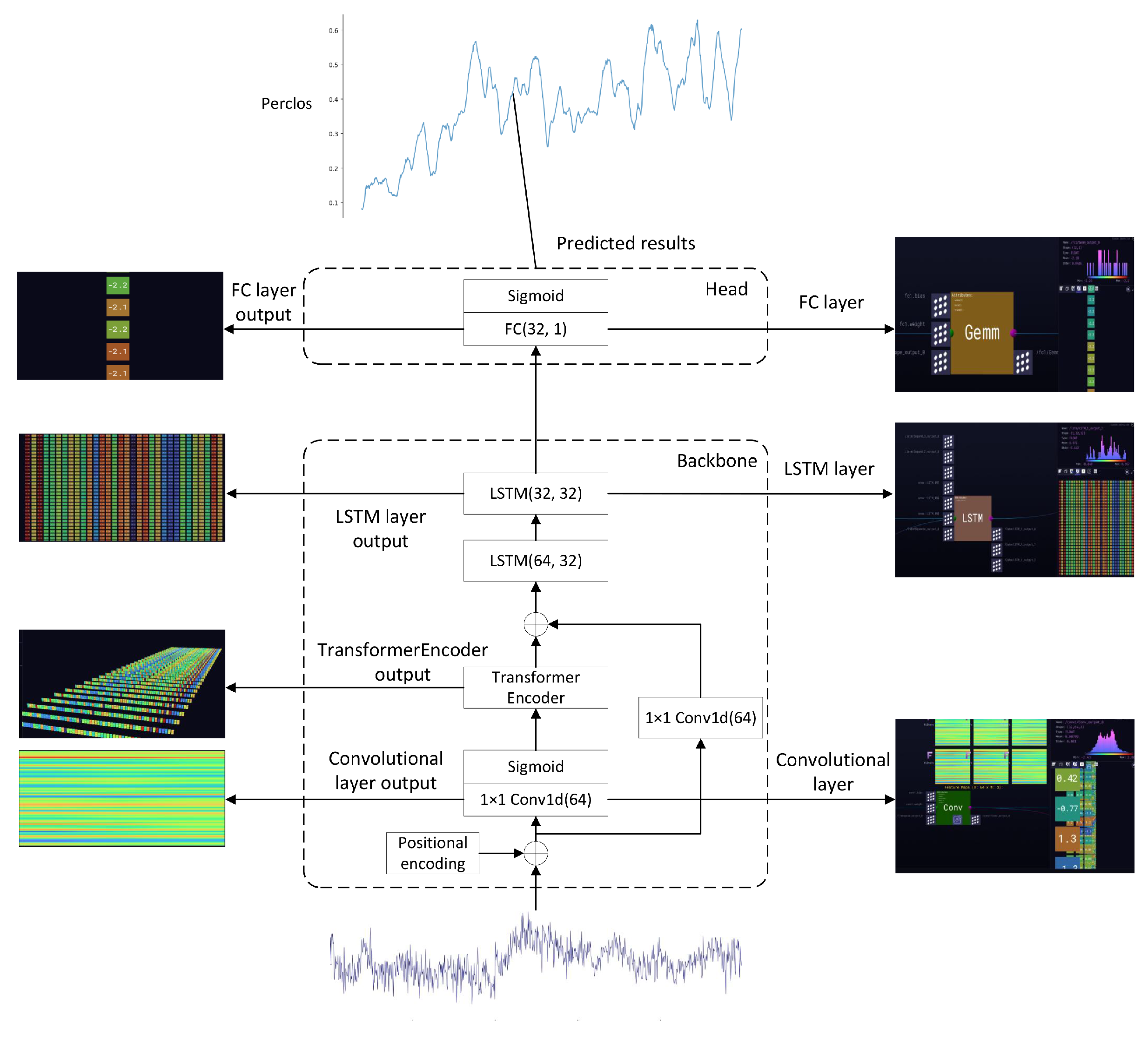
The model employs a CNN for dimensionality reduction of input data, utilizes the Transformer encoder architecture to capture diverse features and relationships within sequences, and subsequently feeds the extracted feature sequences into an LSTM network to extract temporal dependencies. Furthermore, residual connections are incorporated to enhance information flow and mitigate gradient vanishing issues. Finally, a fully connected layer performs regression prediction of fatigue states. The model parameters are shown in the following table.

Table 1.
CTL-ResFNet Parameter Information.
| Component | Parameters |
|---|---|
| PositionalEncoding | d_model=86 |
| Conv1d | input=86, output=64, kernel=1 |
| TransformerEncoderLayer | d_model=64, nhead=4, dim_feedforward=64 |
| TransformerEncoder | 1 layer |
| LSTM | input=64, hidden=32, layers=2 |
| FC | input=32, output=1 |
3.2. Position Encoding and Activation Function
Since the Transformer encoder does not inherently capture positional information, sinusoidal positional encoding is employed:
where denotes the input position, is the feature dimension, and i the feature index.
The model uses two nonlinear activation functions: ReLU and Sigmoid. ReLU is defined as
which maintains a gradient of 1 for positive inputs, mitigating gradient vanishing in deep networks.
The Sigmoid function,
outputs values in , making it suitable for probability prediction.
3.3. CNN Module
Convolutional Neural Networks (CNN) were first proposed by Yann LeCun et al. [19] in 1998, primarily for image processing. CNNs have since been extended to handle one-dimensional data, such as time series. In this study, we employ a one-dimensional CNN (1D CNN) architecture, where convolution kernels slide along the input sequence to compute dot products of local regions.
Figure 2 illustrates the convolutional kernel used in this study. It operates on individual elements of the input data, producing output with the same spatial dimensions but cannot capture relationships between adjacent elements. This operation is applied to multi-channel input for dimensionality reduction: as shown in Figure 3, a 1D convolution with size 1 transforms a 3-channel input into a 2-channel output without altering sequence length.
3.4. Transformer Encoder Module
In 2017, Vaswani et al. [20] introduced the Transformer architecture, consisting of an encoder and a decoder. In this study, only the Transformer encoder is employed, as shown in Figure 4.
The Transformer encoder is composed of n stacked layers ( in this study), each containing two sub-layers: a multi-head self-attention mechanism followed by layer normalization and residual connection, and a position-wise feed-forward network with similar normalization and residual structure.
The scaled dot-product attention is defined as:
where Q, K, and V are query, key, and value vectors, and is the key dimension.
Multi-head attention enables capturing diverse feature representations:
where are learnable weights.
The feed-forward network enhances model capacity:
Residual connections [21] mitigate vanishing/exploding gradients:
Layer normalization stabilizes training by reducing internal covariate shift, normalizing inputs across channels.
3.5. LSTM Module
Long Short-Term Memory (LSTM), proposed by Hochreiter and Schmidhuber in 1997 [22], is a variant of traditional RNNs with superior ability to capture long-range dependencies in sequential data. LSTM architectures have been successfully applied to fatigue detection tasks [23].
An LSTM unit relies on four key components: the forget gate, input gate, cell state, and output gate. Figure 5 illustrates the internal structure of a single LSTM unit. At timestep t, the unit receives the input and the previous hidden state , producing an updated cell state and hidden state , which are then propagated to the next timestep.
The forget gate decides which historical information to discard:
The input gate determines how much new information to store:
The cell state is updated as:
The output gate controls the hidden state output:
This simplified structure shows how LSTM selectively remembers or forgets information, enabling effective modeling of long-range dependencies in sequential data.
3.6. Regression Prediction Head
The hidden state output from the final timestep of the LSTM layer in the feature extraction backbone network is connected to the regression prediction head. The regression head consists of a fully connected (FC) layer with an input dimension of 32 and an output dimension of 1. Since the output values are constrained within the range (0,1), a sigmoid activation function is employed.
4. Experiments
4.1. SEED-VIG Dataset
EEG signals represent the scalp-recorded electrical potentials generated by synchronous discharges of neuronal populations, primarily originating from the synchronized synaptic activities of pyramidal cells in the cerebral cortex [24]. Specifically, the human brain contains tens of thousands of interconnected neurons. These neurons receive signals from other neurons and generate EEG signals when the received signals exceed a certain threshold. Essentially, brain waves represent the electrical signals produced by the collective activity of these neurons. Single-channel EEG signals provide limited information with poor determinacy, leading to random research outcomes, whereas multi-channel EEG signals can capture more comprehensive information and better reflect global brain activities. EEG signals possess inherent non-replicability as physiological characteristics. Relevant studies have demonstrated significant differences in EEG patterns between fatigue and non-fatigue states [25]. Among various physiological indicators for fatigue assessment, EEG signals are recognized as one of the most reliable biomarkers [26]. Researchers have made notable breakthroughs in monitoring fatigue levels by leveraging EEG signal analysis. [27,28,29].
The SEED-VIG database [30], a benchmark for driver fatigue studies, was adopted in this work. Developed by Shanghai Jiao Tong University’s Brain-Inspired Computing team, it includes data from 23 subjects (mean age: 23.3 years). Experiments were conducted in a virtual driving simulator with a projected road scene. The 118-minute experimental sessions were primarily scheduled in the afternoon to facilitate fatigue induction. Participants wore EEG caps for electrophysiological signal acquisition and SMI gaze-tracking apparatus to measure eye movements, with PERCLOS values calculated for fatigue-level annotation. EEG recordings in the SEED-VIG dataset were obtained at 1000 Hz sampling rate from 17 standard channels referenced to CPZ, covering frontal to occipital areas (FT7, FT8, T7, T8, TP7, TP8, CP1, CP2, P1, PZ, P2, PO3, POZ, PO4, O1, OZ, O2). Figure 6 illustrates the schematic configuration of these 17 electrode positions.
The amplitude of EEG signals is at the microvolt level, making them highly susceptible to interference from various noise sources [31]. Consequently, the acquired data consists of both EEG signals and diverse noise components, with all non-EEG signals collectively referred to as artifacts [32]. The EEG signals were initially processed using a 1-75 Hz bandpass filter for noise suppression, with the sampling rate subsequently de-creased to 200 Hz to optimize computational efficiency. During the feature extraction stage, power spectral density (PSD) and DE features were extracted from EEG sig-nals across five frequency bands (: 1–4 Hz, : 4–8 Hz, : 8–14 Hz, : 14–31 Hz, and : 31–50 Hz). These features were computed using short-time Fourier transform (STFT) with non-overlapping 8-second windows. Additionally, features were extracted across the entire 1-50 Hz frequency band with a 2 Hz resolution. PSD reflects the energy distribution of EEG signals across different frequency bands, which has been demonstrated to be highly correlated with fatigue and drowsiness [33,34,35]. DE, characterizing the complexity and uncertainty of EEG signals, can be regarded as a complexity feature. Studies have shown that various entropy-based and complexity measurement methods can effectively identify fatigue states [36]. Notably, empirical evidence suggests that differential entropy features outperform power spectral density in fatigue detection [15].
One of the most significant manifestations of fatigue is reflected in the eyes [37], where the PERCLOS demonstrates a robust association with fatigue levels. PERCLOS is measured as the duration during which the eyelids cover the pupils within a given period, providing an objective metric for fatigue assessment with its computational formula given in Equation 17.
where is the eyelid closure time within the given time window, and is the total observation time window.In the experiment, PERCLOS was computed over non-overlapping 8-second windows ( s), generating 885 time steps in total. The PERCLOS metric is bounded by 0 and 1, where elevated scores correspond to increased fatigue, which can be interpreted as the proba-bility of driver fatigue. Based on reference [30], the fatigue states were classified as: alert [0, 0.35], fatigued [0.35, 0.7], and drowsy [0.7, 1].
4.2. Evaluation Metrics
Model performance was evaluated using both RMSE and MAE metrics, calculated as follows:
In the above, is the true value, is the predicted value, and m is the number of samples.
The RMSE measures the square root of the average squared differences between predicted and actual values. It penalizes larger errors more heavily, making it particularly sensitive to outliers. Therefore, RMSE reflects the overall deviation magnitude of the model predictions.
The MAE represents the average of the absolute differences between predicted and actual values. It provides a more intuitive interpretation of prediction accuracy, as it directly reflects the average prediction deviation without disproportionately amplifying large errors.
In summary, MAE indicates the average level of prediction error, while RMSE emphasizes the influence of large errors. Using both metrics together provides a comprehensive evaluation of the prediction performance.
4.3. Implementation Details
4.3.1. LOOCV Experiment
The experiment employs LOOCV to evaluate the model’s generalization performance on new subjects. The core concept is that each time one subject is selected as the test set, while all remaining subjects form the training set. This process is repeated until every subject has served as the test set once, and finally, all test results are aggregated for comprehensive evaluation. Subject order is shuffled across participants during training, with within-subject temporal continuity strictly maintained.
4.3.2. Cross-Subject Pre-Training with Within-Subject Fine-Tuning Experiment
The experiment adopts a two-stage training strategy, consisting of a pre-training stage and a fine-tuning stage. This study falls within the scope of transfer learning, which has demonstrated exceptional cross-task and cross-domain adaptation capabilities across multiple fields including computer vision, natural language processing, and biomedical signal analysis, with its effectiveness being extensively validated [38,39,40,41,42,43].
During the pre-training stage, the training sets of all 23 samples are combined into a unified pre-training dataset, and the order of the training sets is randomly shuffled each epoch while preserving the internal temporal sequence of each sample. Early stopping is monitored simultaneously using the validation sets of all 23 samples during pre-training. In the fine-tuning stage, the pre-trained weights obtained from the pre-training stage are used to fine-tune the parameters for individual samples, with each sample’s training set utilized for fine-tuning. Early stopping is monitored using the respective sample’s validation set, and the final evaluation is performed on the sample’s test set. This cross-subject to within-subject hybrid design enables simultaneous learning of population-level common features and adaptation to individual variations.
This study constructs an EEG dataset by concatenating DE and eyelid closure degree at the feature level. Let the differential entropy matrix be , the eyelid closure vector be , and the concatenated dataset be . Subsequently, a sliding window is constructed for the dataset , using the previous three time steps to predict the next time step. Time step 3 is the optimal solution obtained through comparative experiments(Table 2). The 23 time-series data samples are split into training, validation, and test sets in an 8:1:1 ratio, without shuffling the temporal order. The training set is used for model training, the validation set for monitoring the training process in combination with an early-stopping strategy, and the test set for the final evaluation of model performance. For each i in the training, validation, and test sets:
To eliminate dimensional and scale differences while accelerating model convergence, this study processes the data using Z-score standardization, scaling the data to follow a standard normal distribution. The calculation formula is as follows:
corresponds to the mean, and to the standard deviation.
4.3.3. Additional Feature Extraction
To further explore the discriminative patterns in EEG signals, we extracted three additional features from the raw EEG data in the SEED-VIG dataset: the / band power ratio, wavelet entropy, and Hurst exponent. Prior to feature extraction, the raw EEG data underwent preprocessing involving 1-75Hz bandpass filtering and artifact removal through Independent Component Analysis (ICA). These procedures were implemented using the EEGLAB toolbox, a MATLAB toolkit specifically designed for EEG signal processing.
Filtering effectively extracts fatigue-related frequency bands while suppressing signal interference. As shown in Figure 7, the filtered power spectral density exhibits significant attenuation beyond 75 Hz.
ICA is an effective method for blind source separation [44], which enables the isolation of interference signals unrelated to fatigue, such as EOG and electromyographic (EMG) signals. As illus-trated in Figure 8, the ICA-derived results comprise 17 components, among which some represent genuine EEG signals while others constitute artifacts. For subsequent analysis, it is essential to remove these artifactual components while retaining the purified EEG signals.
A representative example of artifacts is shown in Figure 9, where EMG signals are illustrated-with the left panel displaying the topographic brain map and the right panel presenting the time-domain representation of EMG artifacts.
A comparison between the raw EEG signals and preprocessed EEG signals is shown in Figure 10, where the blue waveforms represent the original EEG data and the red waveforms denote the preprocessed EEG signals.
After preprocessing the raw EEG signals to obtain clean electrophysiological data, we subsequently extracted three key EEG features for analysis: the / band power ratio, wavelet entropy, and Hurst exponent. Below we provide a brief introduction to each of these features.
Band power ratio, a commonly used quantitative metric in EEG signal analysis, reflects the activity intensity of different frequency bands. Typically, EEG signals are divided into five frequency bands. The band is associated with relaxation and eye-closed states, while the band correlates with concentration and cognitive activities. A high ratio is commonly observed during relaxed or meditative states. An increased ratio indicates mental fatigue. This ratio is calculated as the power ratio between the and bands. In this study, the ratio was computed using STFT with non-overlapping 8-second windows. The formula for calculating the band power ratio is as follows:
Wavelet Entropy [45] is a signal analysis method that combines wavelet transform and information entropy to quantify signal complexity. The wavelet entropy value decreases when the EEG signal exhibits regular and ordered patterns, whereas it increases when the signal becomes complex and disordered. To compute wavelet entropy, the signal is first decomposed using wavelet transform to obtain wavelet coefficients at different scales. The energy at each scale j is then calculated, followed by the determination of relative energy . Finally, wavelet entropy is derived using Shannon’s entropy formula as follows:
This study employs non-overlapping 8-second windows for wavelet transformation using db4 (Daubechies 4) as the mother wavelet with a 5-level decomposition. The , , , , and frequency bands were extracted, and wavelet entropy was subsequently calculated based on these five frequency bands.
The Hurst exponent was originally proposed by hydrologist Harold Hurst [46] and has since been widely applied across various disciplines. This metric quantifies the long-range dependence or self-similarity of EEG signals, thereby reflecting the complexity of brain activity. During fatigue states, the complexity of neural activity decreases while the regularity of EEG signals increases—changes that can be effectively captured by the Hurst exponent. In this study, we performed 5-level decomposition using db4 wavelets for each 8-second non-overlapping window per channel. The reconstructed signals from each frequency band were subsequently analyzed using the rescaled range (R/S) analysis to compute their respective Hurst exponents. The calculation formula for the Hurst exponent is as follows:
The formula parameters are defined as follows: R represents the rescaled range, S denotes the standard deviation of the time series, T indicates the time span (number of data points) of the series, and H is the Hurst exponent whose value typically ranges between
4.4. Training Settings
4.4.1. LOOCV Experiment
The experiment was conducted using the PyTorch framework on an NVIDIA RTX 3050 GPU. During the training process, the MSE loss function was used, with the Adam [47] optimizer, an initial learning rate of 0.001, a batch size of 64, and a fixed number of 20 training epochs.
4.4.2. Cross-Subject Pre-Training with Within-Subject Fine-Tuning Experiment
In the pre-training phase, the Adam optimizer was used with an initial learning rate of 0.001, and the learning rate was dynamically adjusted—halved if the validation loss did not decrease for 5 epochs. The total number of training epochs was 150, and an early stopping mechanism was employed, terminating the training if the validation loss showed no improvement for 10 epochs. The batch size was set to 64. Using the MSE loss function. In the fine-tuning phase, the model was trained for 50 epochs with a learning rate of 0.0001, while all other training configurations remained consistent with those used in the pre-training phase.
4.5. Main Results
4.5.1. Window Length Experiment
From the average results (Avg), a window length of 3 performed the best (RMSE = 0.0598, MAE = 0.0509), with the lowest error. This indicates that for fatigue detection based on EEG (DE features) + PERCLOS, selecting an appropriate time window can significantly improve the model’s prediction accuracy.
Table 2.
Experimental Study on Window Length Selection Based on LSTM (LOOCV Experiment, EEG+PERCLOS).
Table 2.
Experimental Study on Window Length Selection Based on LSTM (LOOCV Experiment, EEG+PERCLOS).
| sub | Window length 1 | Window length 2 | Window length 3 | Window length 4 | Window length 5 | |||||
| RMSE | MAE | RMSE | MAE | RMSE | MAE | RMSE | MAE | RMSE | MAE | |
| 1 | 0.1154 | 0.1004 | 0.1131 | 0.0974 | 0.0768 | 0.0652 | 0.0793 | 0.0711 | 0.0733 | 0.0630 |
| 2 | 0.0493 | 0.0393 | 0.0481 | 0.0414 | 0.0356 | 0.0302 | 0.0830 | 0.0723 | 0.0283 | 0.0213 |
| 3 | 0.0861 | 0.0767 | 0.0778 | 0.0728 | 0.0469 | 0.0407 | 0.0523 | 0.0489 | 0.0935 | 0.0870 |
| 4 | 0.0531 | 0.0433 | 0.1000 | 0.0844 | 0.0443 | 0.0371 | 0.0508 | 0.0417 | 0.0754 | 0.0664 |
| 5 | 0.0572 | 0.0468 | 0.0636 | 0.0564 | 0.0730 | 0.0651 | 0.0710 | 0.0619 | 0.0817 | 0.0724 |
| 6 | 0.0888 | 0.0659 | 0.0615 | 0.0488 | 0.0582 | 0.0429 | 0.0625 | 0.0467 | 0.0741 | 0.0611 |
| 7 | 0.1650 | 0.1161 | 0.1764 | 0.1170 | 0.0526 | 0.0445 | 0.1352 | 0.1010 | 0.0910 | 0.0698 |
| 8 | 0.0580 | 0.0479 | 0.0305 | 0.0249 | 0.0672 | 0.0622 | 0.0463 | 0.0436 | 0.0524 | 0.0492 |
| 9 | 0.1202 | 0.1091 | 0.1809 | 0.1655 | 0.0566 | 0.0538 | 0.0378 | 0.0327 | 0.0549 | 0.0518 |
| 10 | 0.0343 | 0.0276 | 0.0413 | 0.0319 | 0.0545 | 0.0411 | 0.0351 | 0.0269 | 0.0377 | 0.0295 |
| 11 | 0.0235 | 0.0183 | 0.0418 | 0.0323 | 0.0365 | 0.0281 | 0.0474 | 0.0439 | 0.0498 | 0.0467 |
| 12 | 0.0486 | 0.0440 | 0.0438 | 0.0393 | 0.0451 | 0.0394 | 0.0474 | 0.0435 | 0.0482 | 0.0448 |
| 13 | 0.0321 | 0.0283 | 0.0384 | 0.0307 | 0.0707 | 0.0649 | 0.0622 | 0.0578 | 0.0822 | 0.0750 |
| 14 | 0.0828 | 0.0675 | 0.0843 | 0.0689 | 0.0692 | 0.0566 | 0.0635 | 0.0512 | 0.0637 | 0.0520 |
| 15 | 0.1075 | 0.0990 | 0.0575 | 0.0511 | 0.0706 | 0.0607 | 0.0499 | 0.0425 | 0.0684 | 0.0604 |
| 16 | 0.0677 | 0.0567 | 0.0719 | 0.0600 | 0.0497 | 0.0433 | 0.0464 | 0.0372 | 0.0591 | 0.0510 |
| 17 | 0.0555 | 0.0502 | 0.0442 | 0.0377 | 0.0483 | 0.0438 | 0.0547 | 0.0493 | 0.0466 | 0.0416 |
| 18 | 0.0600 | 0.0490 | 0.1009 | 0.0876 | 0.0789 | 0.0704 | 0.0687 | 0.0602 | 0.0698 | 0.0621 |
| 19 | 0.0573 | 0.0446 | 0.0573 | 0.0495 | 0.0709 | 0.0596 | 0.0627 | 0.0501 | 0.0668 | 0.0559 |
| 20 | 0.0918 | 0.0719 | 0.0927 | 0.0713 | 0.0827 | 0.0688 | 0.0619 | 0.0531 | 0.0569 | 0.0482 |
| 21 | 0.0365 | 0.0336 | 0.0436 | 0.0339 | 0.0581 | 0.0522 | 0.1008 | 0.0791 | 0.0389 | 0.0363 |
| 22 | 0.0759 | 0.0628 | 0.0719 | 0.0491 | 0.0528 | 0.0425 | 0.0553 | 0.0414 | 0.0746 | 0.0573 |
| 23 | 0.0821 | 0.0711 | 0.0605 | 0.0506 | 0.0764 | 0.0574 | 0.0495 | 0.0412 | 0.0559 | 0.0435 |
| Avg | 0.0717 | 0.0596 | 0.0740 | 0.0609 | 0.0598 | 0.0509 | 0.0619 | 0.0521 | 0.0627 | 0.0542 |
4.5.2. Comparison of Univariate and Multimodal Fatigue Prediction Based on LSTM
This study employs an LSTM model for fatigue state prediction and designs two comparative experiments based on a LOOCV paradigm: the first group uses univariate modeling based solely on PERCLOS (PERCLOS-only), while the second group employs multimodal fusion modeling combining EEG signals (DE features) and PERCLOS (EEG + PERCLOS). As shown in Table 3, the prediction performance of the multimodal fusion model (Avg RMSE = 0.0598) is significantly better than that of the univariate model (Avg RMSE = 0.0683), with a relative error reduction of 12.4%. These results confirm the effectiveness of multimodal physiological signal fusion in fatigue state recognition, demonstrating that EEG features and PERCLOS indicators exhibit complementarity, and their joint modeling can improve prediction accuracy.
4.5.3. Cross-Subject Generalization and Individual Adaptation Analysis
This study systematically validated the superior performance of the CTL-ResFNet model through LOOCV experiments and pretraining-finetuning comparison experiments. The experiments selected CNN, Transformer, LSTM, and CNN-Transformer as baseline models for comparative analysis. As shown in Table 4, in the LOOCV, CTL-ResFNet achieved an average RMSE of 0.0266 and an average MAE of 0.0215, significantly outperforming all comparative models. This result fully demonstrates the model’s exceptional generalization capability in zero-shot cross-subject scenarios, highlighting its unique architectural advantages. Further fine-tuning experimental results (Table 5) revealed that CTL-ResFNet (Avg RMSE = 0.0935) also exhibited significant advantages in individual adaptation ability, further validating the model’s strong transferability and adaptability.
4.5.4. Comparison of Feature Performance Between LOOCV and Fine-Tuning Experiments
This study further extracted three feature indicators from EEG signals: the / band power ratio, wavelet entropy, and Hurst exponent. Two experimental paradigms—LOOCV and pretraining-finetuning (based on the CTL-ResFNet framework)—were employed for validation. As shown in Table 6, under the LOOCV setting, the / band power ratio demonstrated the best predictive performance, achieving an average RMSE of 0.0190. In contrast, in the pretraining-finetuning experiments presented in Table 7, the DE feature performed the best, with an average RMSE of 0.0935. This comparative result indicates that the optimal feature selection varies significantly under different validation paradigms, suggesting that the most suitable feature indicators should be chosen based on the specific experimental design in practical applications.
5. Conclusions
This paper introduces CTL-ResFNet, a novel deep learning model that integrates CNN, TransformerEncoder, LSTM, and residual connections to predict driver fatigue using historical EEG signals and PERCLOS. By effectively capturing spatiotemporal dependencies in EEG data, the proposed model outperforms baseline approaches (CNN, Transformer, LSTM, and CNN-Transformer) in both LOOCV and pretraining-finetuning experiments, as reflected by lower RMSE and MAE values.
Results demonstrate that combining EEG-based DE features with PERCLOS substantially improves fatigue prediction accuracy compared to using PERCLOS alone, as confirmed through LSTM validation experiments. Comparative analysis of alternative EEG features—including the / band power ratio, wavelet entropy, and Hurst exponent—reveals that while the / ratio performs best in cross-validation, DE features exhibit superior effectiveness in pretraining-finetuning scenarios, highlighting the need for context-aware feature selection.
These findings emphasize the promise of multimodal deep learning for fatigue monitoring, with CTL-ResFNet providing a robust framework for real-world deployment. Future research directions could include enhancing model interpretability and incorporating additional physiological signals to further improve performance.
Author Contributions
Conceptualization, Zhanyang Wang and Xin Du; methodology, Zhanyang Wang; software, Zhanyang Wang; validation, Zhanyang Wang, Chengbin Jiang and Junyang Sun; formal analysis, Zhanyang Wang; investigation, Chengbin Jiang and Junyang Sun; resources, Xin Du; data curation, Zhanyang Wang; writing—original draft preparation, Zhanyang Wang; writing—review and editing, Xin Du; visualization, Zhanyang Wang; supervision, Xin Du; project administration, Xin Du. All authors have read and agreed to the published version of the manuscript.
Funding
This research received no external funding
Institutional Review Board Statement
Not applicable
Informed Consent Statement
Not applicable
Data Availability Statement
The data analyzed in this study were sourced from the SEED-VIG dataset provided by Shanghai Jiao Tong University, accessible at: https://bcmi.sjtu.edu.cn/home/seed/seed-vig.html. This dataset is subject to access restrictions and requires submitting an application to the data provider for approval prior to use.
Conflicts of Interest
The authors declare no conflicts of interest.
Appendix A
Appendix A.1
Figure A1.
Prediction performance of each model in the LOOCV experiment, with the horizontal axis representing the time steps (a total of 885 time steps, each separated by 8s) and the vertical axis representing PERCLOS.
Figure A1.
Prediction performance of each model in the LOOCV experiment, with the horizontal axis representing the time steps (a total of 885 time steps, each separated by 8s) and the vertical axis representing PERCLOS.
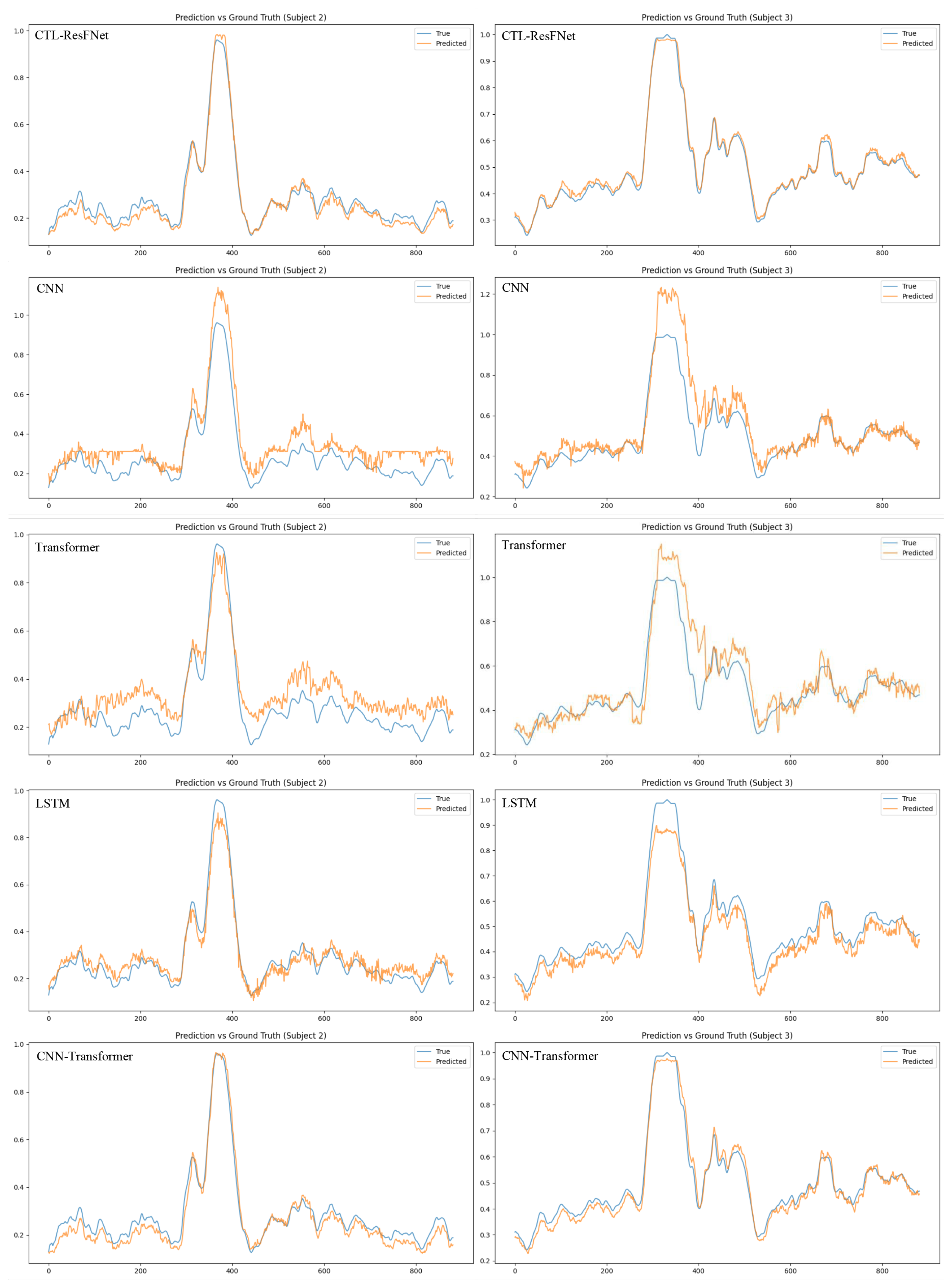
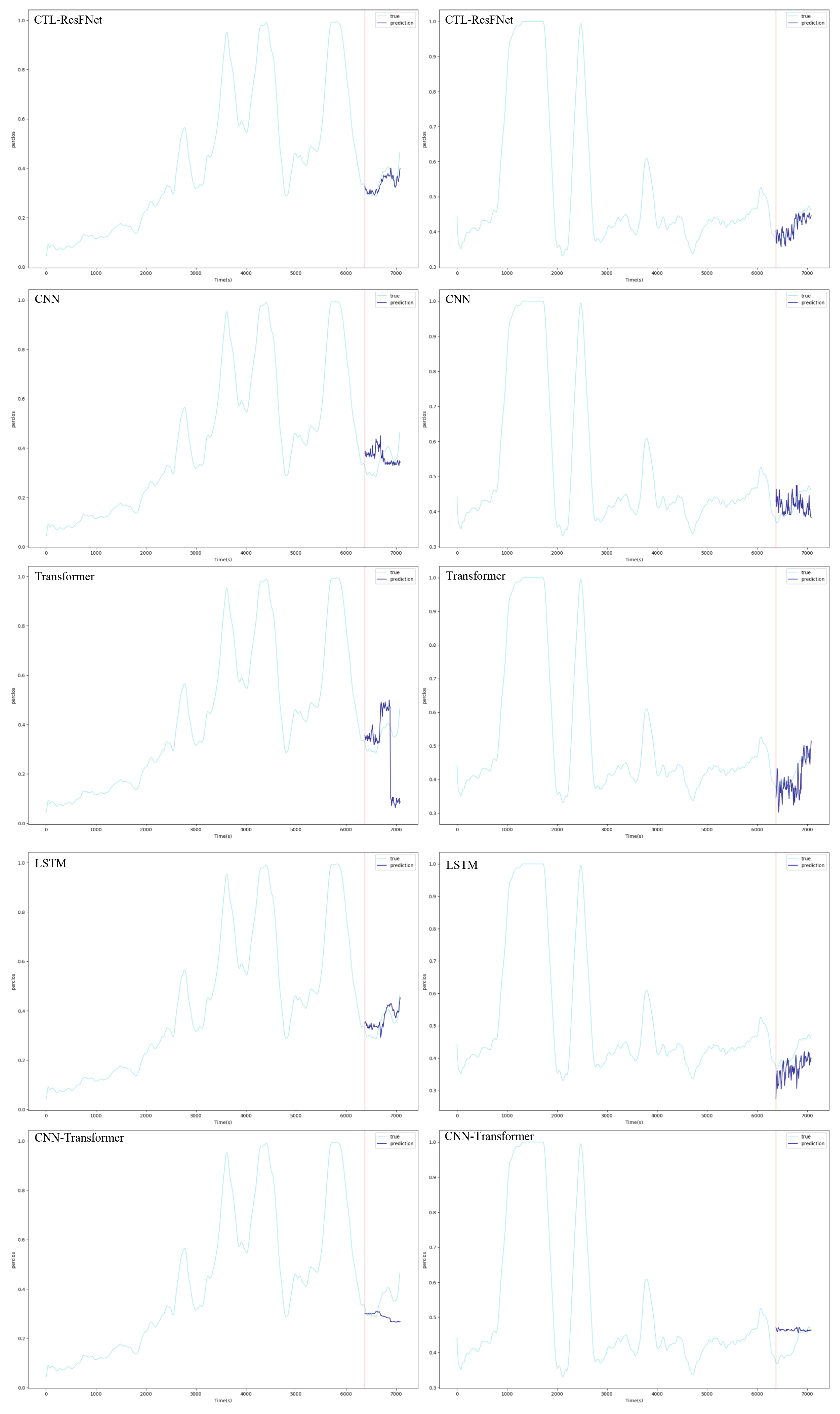
Figure A2.
Prediction results of each model in the pre-training and fine-tuning experiment, with the x-axis representing time in seconds (total 7080s) and the y-axis representing PERCLOS (Subject 7 left and Subject 19 right).
Figure A2.
Prediction results of each model in the pre-training and fine-tuning experiment, with the x-axis representing time in seconds (total 7080s) and the y-axis representing PERCLOS (Subject 7 left and Subject 19 right).
References
- Khunpisuth O, Chotchinasri T, Koschakosai V, et al. Driver drowsiness detection using eye-closeness detection [C]. In 2016 12th International Conference on Signal-Image Technology & Internet-Based Systems (SITIS), 2016: 661–668.
- Fan J, Smith A P. A preliminary review of fatigue among rail staff [J]. Frontiers in psychology, 2018, 9: 634. [CrossRef]
- Ahmed M, Masood S, Ahmad M, et al. Intelligent driver drowsiness detection for traffic safety based on multi CNN deep model and facial subsampling [J]. IEEE transactions on intelligent transportation systems, 2021, 23 (10): 19743–19752. [CrossRef]
- Yogarajan G, Singh R N, Nandhu S A, et al. Drowsiness detection system using deep learning based data fusion approach [J]. Multimedia Tools and Applications, 2024, 83 (12): 36081–36095. [CrossRef]
- Gao Z, Chen X, Xu J, et al. Semantically-Enhanced Feature Extraction with CLIP and Transformer Networks for Driver Fatigue Detection [J]. Sensors, 2024, 24 (24): 7948. [CrossRef]
- Ganguly B, Dey D, Munshi S. An Attention Deep Learning Framework-Based Drowsiness Detection Model for Intelligent Transportation System [J]. IEEE Transactions on Intelligent Transportation Systems, 2025. [CrossRef]
- Lyu X, Akbar M A, Manimurugan S, et al. Driver Fatigue Warning Based on Medical Physiological Signal Monitoring for Transportation Cyber-Physical Systems [J]. IEEE Transactions on Intelligent Transportation Systems, 2025.
- Wang K, Mao X, Song Y, et al. EEG-based fatigue state evaluation by combining complex network and frequency-spatial features [J]. Journal of neuroscience methods, 2025, 416: 110385. [CrossRef]
- Åkerstedt T, Torsvall L. Continuous Electrophysiological Recording [J]. Breakdown in Human Adaptation to ‘Stress’ Towards a multidisciplinary approach Volume I, 1984: 567–583.
- Åkerstedt T, Kecklund G, Knutsson A. Manifest sleepiness and the spectral content of the EEG during shift work [J]. Sleep, 1991, 14 (3): 221–225. [CrossRef]
- Eoh H J, Chung M K, Kim S-H. Electroencephalographic study of drowsiness in simulated driving with sleep deprivation [J]. International Journal of Industrial Ergonomics, 2005, 35 (4): 307–320. [CrossRef]
- Jap B T, Lal S, Fischer P, et al. Using EEG spectral components to assess algorithms for detecting fatigue [J]. Expert Systems with Applications, 2009, 36 (2): 2352–2359. [CrossRef]
- Khushaba R N, Kodagoda S, Lal S, et al. Driver drowsiness classification using fuzzy wavelet-packet-based feature-extraction algorithm [J]. IEEE transactions on biomedical engineering, 2010, 58 (1): 121–131. [CrossRef]
- Zhao C, Zheng C, Zhao M, et al. Multivariate autoregressive models and kernel learning algorithms for classifying driving mental fatigue based on electroencephalographic [J]. Expert Systems with Applications, 2011, 38 (3): 1859–1865. [CrossRef]
- Huo X-Q, Zheng W-L, Lu B-L. Driving fatigue detection with fusion of EEG and forehead EOG [C]. In 2016 international joint conference on neural networks (IJCNN), 2016: 897–904.
- Chaabene S, Bouaziz B, Boudaya A, et al. Convolutional neural network for drowsiness detection using EEG signals [J]. Sensors, 2021, 21 (5): 1734. [CrossRef]
- Cui J, Lan Z, Sourina O, et al. EEG-based cross-subject driver drowsiness recognition with an interpretable convolutional neural network [J]. IEEE Transactions on Neural Networks and Learning Systems, 2022, 34 (10): 7921–7933. [CrossRef]
- Shi L-C, Jiao Y-Y, Lu B-L. Differential entropy feature for EEG-based vigilance estimation [C]. In 2013 35th Annual International Conference of the IEEE Engineering in Medicine and Biology Society (EMBC), 2013: 6627–6630.
- LeCun Y, Bottou L, Bengio Y, et al. Gradient-based learning applied to document recognition [J]. Proceedings of the IEEE, 2002, 86 (11): 2278–2324. [CrossRef]
- Vaswani A, Shazeer N, Parmar N, et al. Attention is all you need [J]. Advances in neural information processing systems, 2017, 30.
- He K, Zhang X, Ren S, et al. Deep residual learning for image recognition [C]. In Proceedings of the IEEE conference on computer vision and pattern recognition, 2016: 770–778.
- Hochreiter S, Schmidhuber J. Long short-term memory [J]. Neural computation, 1997, 9 (8): 1735–1780.
- Jiao Y, Deng Y, Luo Y, et al. Driver sleepiness detection from EEG and EOG signals using GAN and LSTM networks [J]. Neurocomputing, 2020, 408: 100–111. [CrossRef]
- Avitan L, Teicher M, Abeles M. EEG generator—a model of potentials in a volume conductor [J]. Journal of neurophysiology, 2009, 102 (5): 3046–3059. [CrossRef]
- Gharagozlou F, Saraji G N, Mazloumi A, et al. Detecting driver mental fatigue based on EEG alpha power changes during simulated driving [J]. Iranian journal of public health, 2015, 44 (12): 1693.
- Panicker R C, Puthusserypady S, Sun Y. An asynchronous P300 BCI with SSVEP-based control state detection [J]. IEEE Transactions on Biomedical Engineering, 2011, 58 (6): 1781–1788. [CrossRef]
- Cui Y, Xu Y, Wu D. EEG-based driver drowsiness estimation using feature weighted episodic training [J]. IEEE transactions on neural systems and rehabilitation engineering, 2019, 27 (11): 2263–2273. [CrossRef]
- Gao Z, Wang X, Yang Y, et al. EEG-based spatio–temporal convolutional neural network for driver fatigue evaluation [J]. IEEE transactions on neural networks and learning systems, 2019, 30 (9): 2755–2763.
- Akin M, Kurt M B, Sezgin N, et al. Estimating vigilance level by using EEG and EMG signals [J]. Neural Computing and Applications, 2008, 17: 227–236. [CrossRef]
- Zheng W-L, Lu B-L. A multimodal approach to estimating vigilance using EEG and forehead EOG [J]. Journal of neural engineering, 2017, 14 (2): 026017. [CrossRef]
- Hu L, Zhang Z. EEG signal processing and feature extraction [M]. Springer, 2019.
- Luck S J. An introduction to the event-related potential technique [M]. MIT press, 2014.
- Wei C-S, Lin Y-P, Wang Y-T, et al. A subject-transfer framework for obviating inter-and intra-subject variability in EEG-based drowsiness detection [J]. NeuroImage, 2018, 174: 407–419. [CrossRef]
- Wei C-S, Wang Y-T, Lin C-T, et al. Toward drowsiness detection using non-hair-bearing EEG-based brain-computer interfaces [J]. IEEE transactions on neural systems and rehabilitation engineering, 2018, 26 (2): 400–406. [CrossRef]
- Liu Y, Lan Z, Cui J, et al. Inter-subject transfer learning for EEG-based mental fatigue recognition [J]. Advanced Engineering Informatics, 2020, 46: 101157.
- Zhang C, Wang H, Fu R. Automated detection of driver fatigue based on entropy and complexity measures [J]. IEEE Transactions on Intelligent Transportation Systems, 2013, 15 (1): 168–177. [CrossRef]
- Sigari M-H, Fathy M, Soryani M. A driver face monitoring system for fatigue and distraction detection [J]. International journal of vehicular technology, 2013, 2013 (1): 263983. [CrossRef]
- Dosovitskiy A, Beyer L, Kolesnikov A, et al. An image is worth 16x16 words: Transformers for image recognition at scale [J]. arXiv preprint arXiv:2010.11929, 2020.
- Panigrahi S, Nanda A, Swarnkar T. A survey on transfer learning [M] // Panigrahi S, Nanda A, Swarnkar T. Intelligent and Cloud Computing: Proceedings of ICICC 2019, Volume 1. Springer, 2020: 2020: 781–789.
- Devlin J, Chang M-W, Lee K, et al. Bert: Pre-training of deep bidirectional transformers for language understanding [C]. In Proceedings of the 2019 conference of the North American chapter of the association for computational linguistics: human language technologies, volume 1 (long and short papers), 2019: 4171–4186.
- Ruder S, Peters M E, Swayamdipta S, et al. Transfer learning in natural language processing [C]. In Proceedings of the 2019 conference of the North American chapter of the association for computational linguistics: Tutorials, 2019: 15–18.
- Maqsood M, Nazir F, Khan U, et al. Transfer learning assisted classification and detection of Alzheimer’s disease stages using 3D MRI scans [J]. Sensors, 2019, 19 (11): 2645. [CrossRef]
- Schweikert G, Rätsch G, Widmer C, et al. An empirical analysis of domain adaptation algorithms for genomic sequence analysis [J]. Advances in neural information processing systems, 2008, 21.
- Hyvärinen A, Oja E. Independent component analysis: algorithms and applications [J]. Neural networks, 2000, 13 (4-5): 411–430. [CrossRef]
- Särkelä M O, Ermes M J, van Gils M J, et al. Quantification of epileptiform electroencephalographic activity during sevoflurane mask induction [J]. Anesthesiology, 2007, 107 (6): 928–938.
- Hurst H. Long-term storage of reservoirs: an experimental study. Transactions of the American society of civil engineers [J], 1951.
- Kingma D P, Ba J. Adam: A method for stochastic optimization [J]. arXiv preprint arXiv:1412.6980, 2014.
Figure 2.
1D CNN(kernel_size=1).
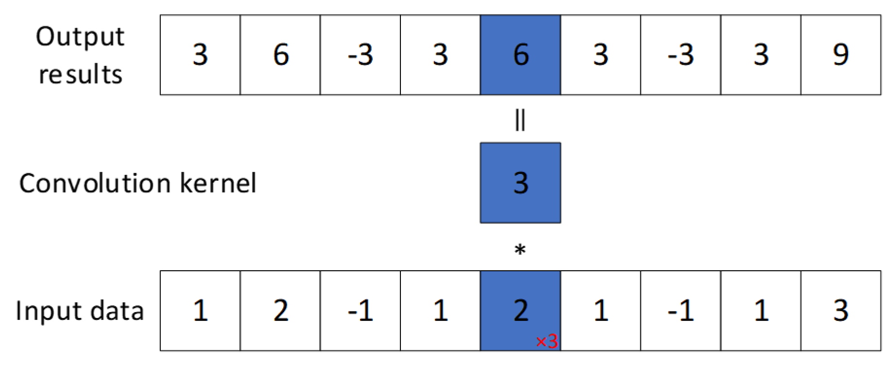
Figure 3.
1D CNN(kernel_size=1, in_channels=3, out_channels=2).
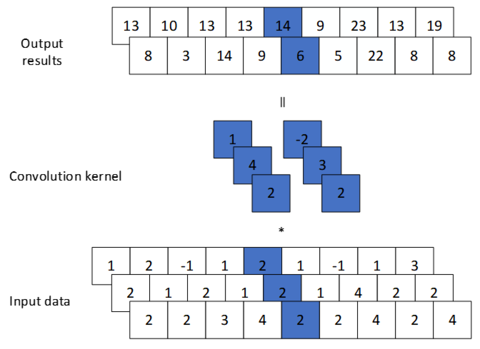
Figure 4.
Transformer Encoder.
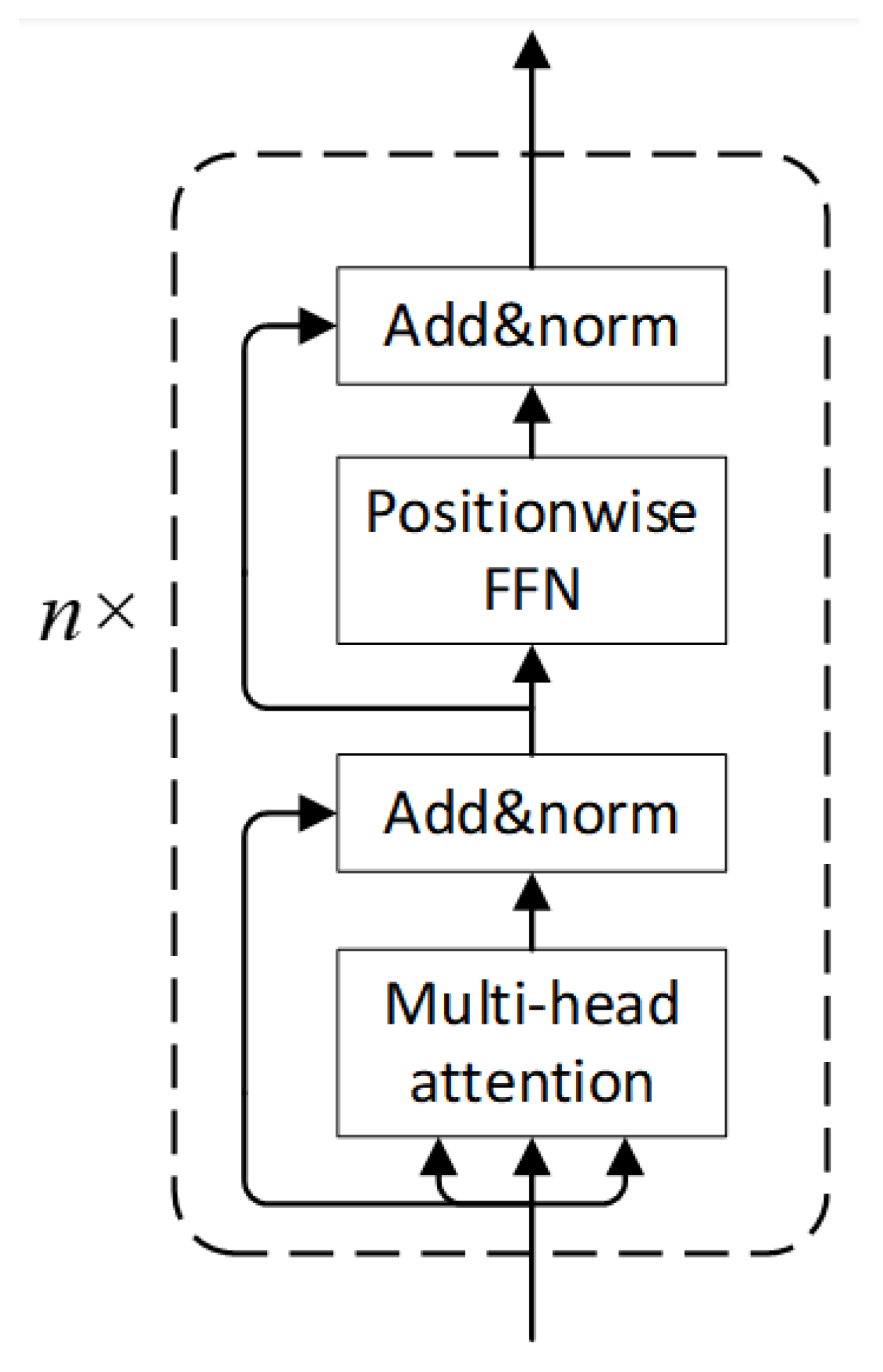
Figure 5.
LSTM structure.
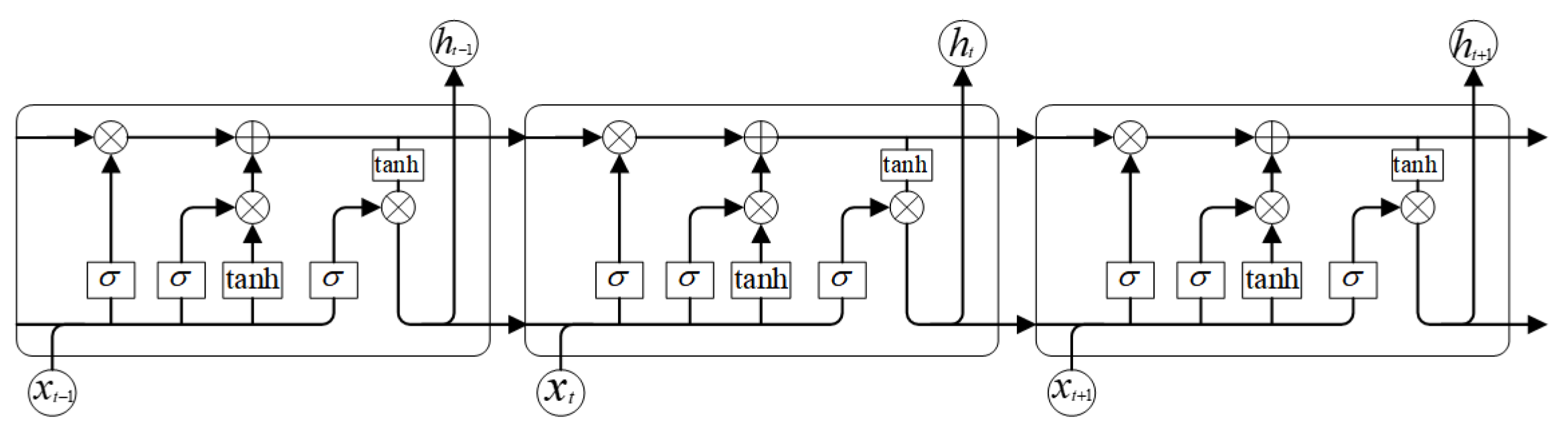
Figure 6.
Schematic diagram of electrode channel and EEG signal acquisition.
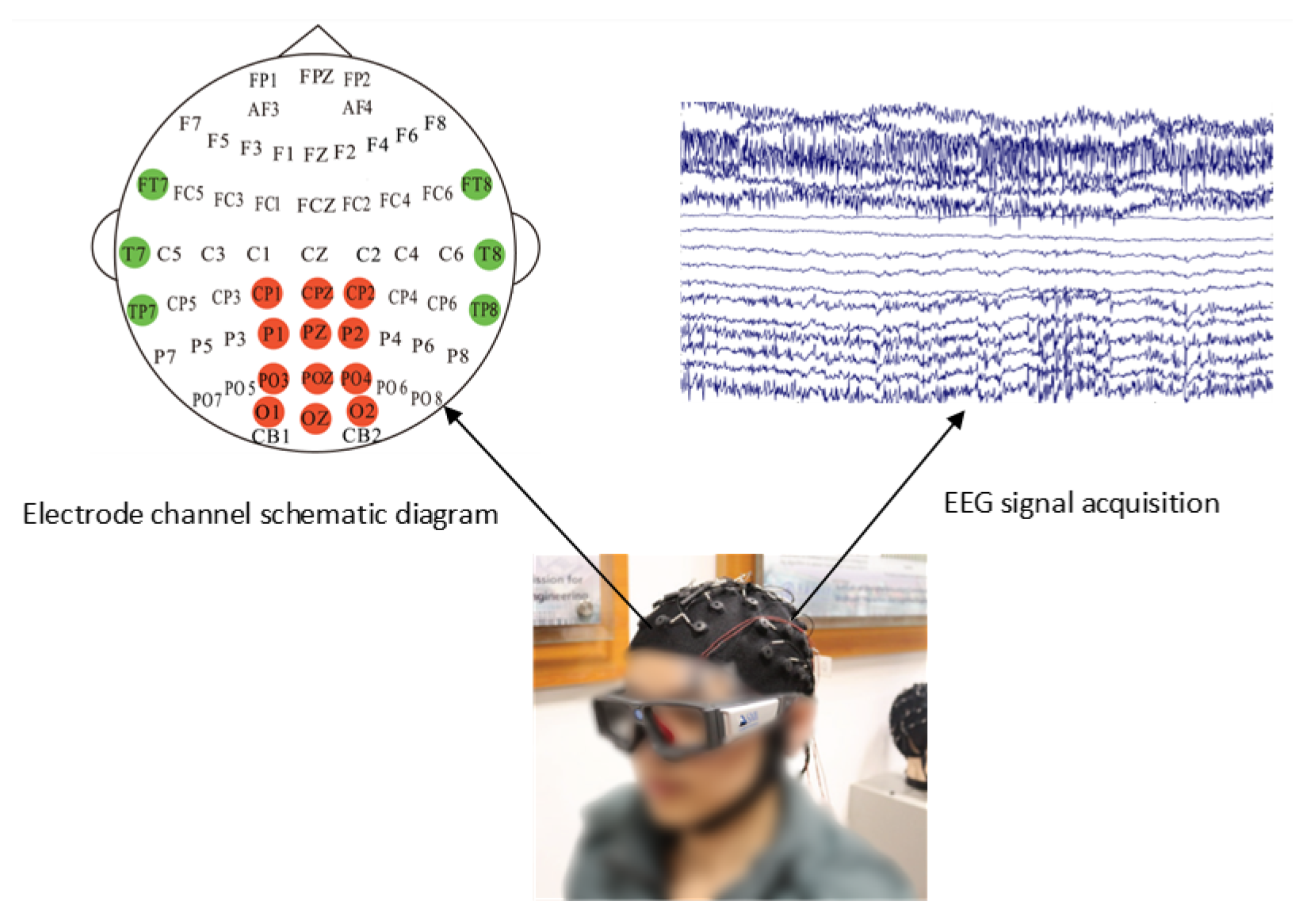
Figure 7.
Power spectral density after 1-75 Hz filtering.
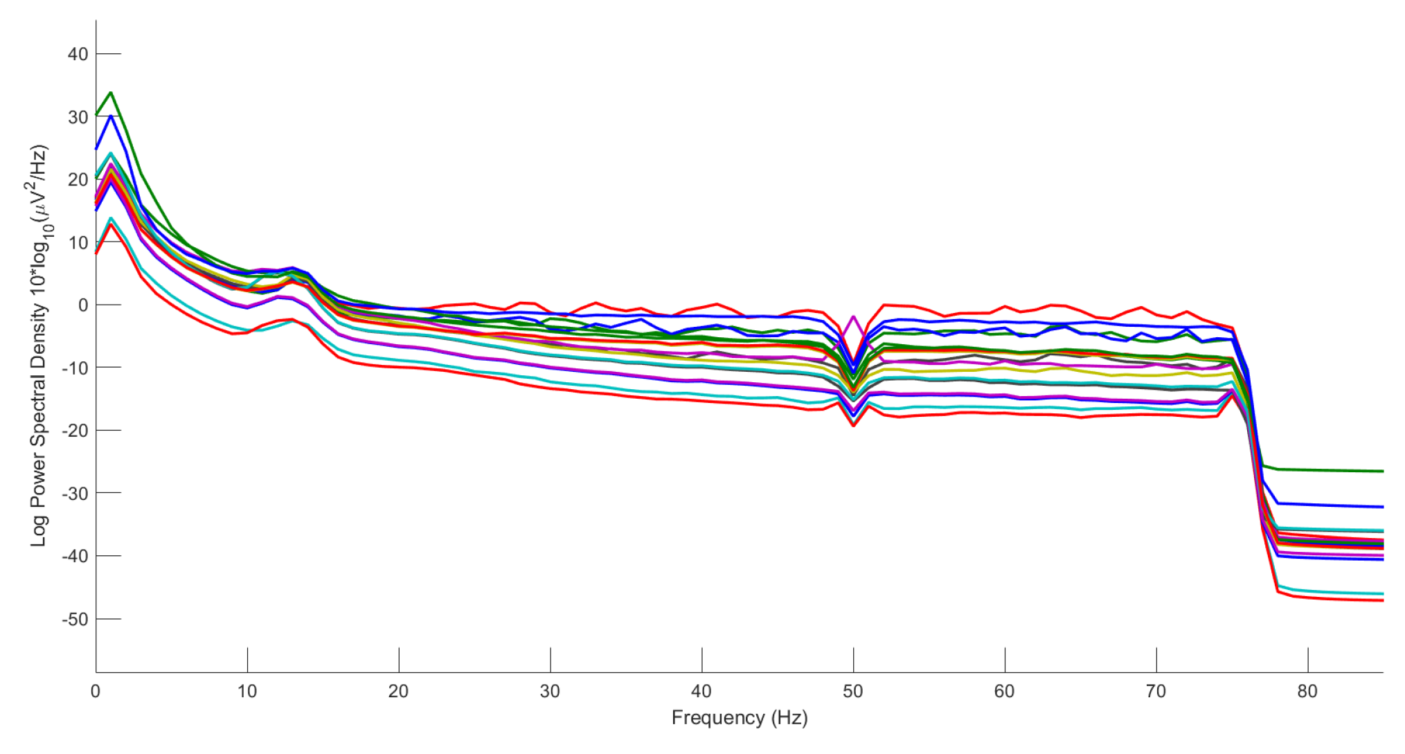
Figure 8.
17 ICA components
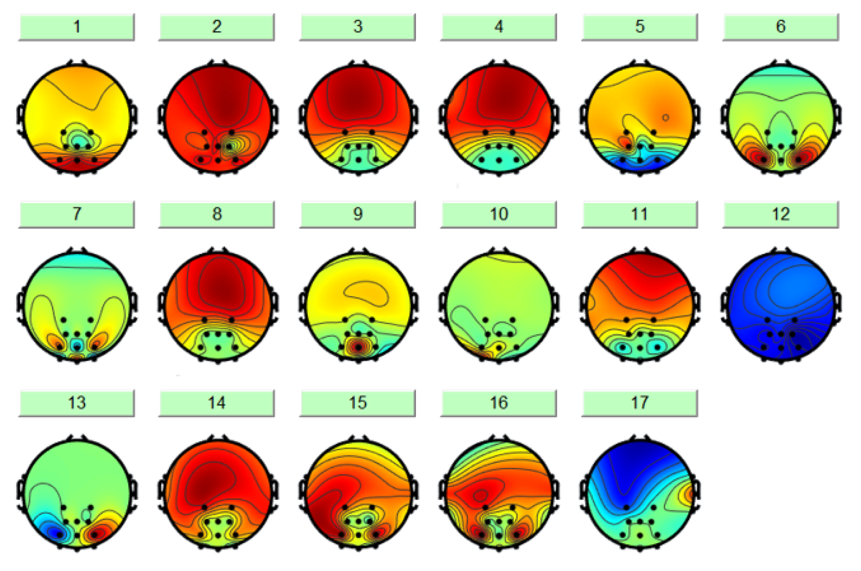
Figure 9.
EMG artifact-related components.
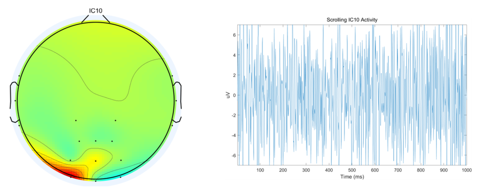
Figure 10.
Comparison of EEG signals before and after preprocessing After preprocessing the raw EEG signals to obtain.
Figure 10.
Comparison of EEG signals before and after preprocessing After preprocessing the raw EEG signals to obtain.
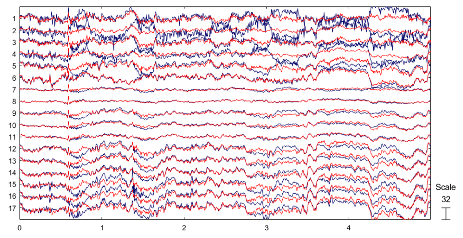
Table 3.
Experimental Comparison of LSTM-based EEG+PERCLOS and PERCLOS-only Approaches (LOOCV Experiment).
Table 3.
Experimental Comparison of LSTM-based EEG+PERCLOS and PERCLOS-only Approaches (LOOCV Experiment).
| sub | EEG+PERCLOS | PERCLOS-only | ||
| RMSE | MAE | RMSE | MAE | |
| 1 | 0.0768 | 0.0652 | 0.0842 | 0.0767 |
| 2 | 0.0356 | 0.0302 | 0.0399 | 0.0335 |
| 3 | 0.0469 | 0.0407 | 0.0595 | 0.0557 |
| 4 | 0.0443 | 0.0371 | 0.0465 | 0.0390 |
| 5 | 0.0730 | 0.0651 | 0.0672 | 0.0575 |
| 6 | 0.0582 | 0.0429 | 0.0852 | 0.0644 |
| 7 | 0.0526 | 0.0445 | 0.0564 | 0.0462 |
| 8 | 0.0672 | 0.0622 | 0.0491 | 0.0458 |
| 9 | 0.0566 | 0.0538 | 0.0520 | 0.0496 |
| 10 | 0.0545 | 0.0411 | 0.0592 | 0.0437 |
| 11 | 0.0365 | 0.0281 | 0.0537 | 0.0502 |
| 12 | 0.0451 | 0.0394 | 0.0542 | 0.0496 |
| 13 | 0.0707 | 0.0649 | 0.0698 | 0.0656 |
| 14 | 0.0692 | 0.0566 | 0.0866 | 0.0703 |
| 15 | 0.0706 | 0.0607 | 0.0861 | 0.0813 |
| 16 | 0.0497 | 0.0433 | 0.0640 | 0.0541 |
| 17 | 0.0483 | 0.0438 | 0.0464 | 0.0416 |
| 18 | 0.0789 | 0.0704 | 0.0802 | 0.0700 |
| 19 | 0.0709 | 0.0596 | 0.0853 | 0.0776 |
| 20 | 0.0827 | 0.0688 | 0.1028 | 0.0843 |
| 21 | 0.0581 | 0.0522 | 0.0706 | 0.0677 |
| 22 | 0.0528 | 0.0425 | 0.0786 | 0.0492 |
| 23 | 0.0764 | 0.0574 | 0.0941 | 0.0581 |
| Avg | 0.0598 | 0.0509 | 0.0683 | 0.0579 |
Table 4.
LOOCV Evaluation Results for Each Model.
| sub | CTL-ResFNet | CNN | Transformer | LSTM | CNN-Transformer | |||||
| RMSE | MAE | RMSE | MAE | RMSE | MAE | RMSE | MAE | RMSE | MAE | |
| 1 | 0.0411 | 0.0362 | 0.0405 | 0.0315 | 0.0589 | 0.0489 | 0.0768 | 0.0652 | 0.0453 | 0.0400 |
| 2 | 0.0257 | 0.0222 | 0.0830 | 0.0715 | 0.0789 | 0.0706 | 0.0356 | 0.0302 | 0.0331 | 0.0289 |
| 3 | 0.0136 | 0.0110 | 0.0873 | 0.0543 | 0.0793 | 0.0519 | 0.0469 | 0.0407 | 0.0239 | 0.0203 |
| 4 | 0.0401 | 0.0302 | 0.1599 | 0.0786 | 0.0792 | 0.0566 | 0.0443 | 0.0371 | 0.0267 | 0.0209 |
| 5 | 0.0256 | 0.0209 | 0.0770 | 0.0649 | 0.1258 | 0.1045 | 0.0730 | 0.0651 | 0.0420 | 0.0338 |
| 6 | 0.0332 | 0.0255 | 0.1426 | 0.1195 | 0.0752 | 0.0573 | 0.0582 | 0.0429 | 0.0337 | 0.0272 |
| 7 | 0.0261 | 0.0153 | 0.4533 | 0.3604 | 0.1719 | 0.1279 | 0.0526 | 0.0445 | 0.0460 | 0.0390 |
| 8 | 0.0231 | 0.0204 | 0.0444 | 0.0331 | 0.0570 | 0.0466 | 0.0672 | 0.0622 | 0.0337 | 0.0275 |
| 9 | 0.0215 | 0.0177 | 0.0260 | 0.0186 | 0.0613 | 0.0478 | 0.0566 | 0.0538 | 0.0559 | 0.0494 |
| 10 | 0.0194 | 0.0165 | 0.0594 | 0.0515 | 0.0846 | 0.0640 | 0.0545 | 0.0411 | 0.0311 | 0.0232 |
| 11 | 0.0415 | 0.0380 | 0.0658 | 0.0571 | 0.0663 | 0.0505 | 0.0365 | 0.0281 | 0.0334 | 0.0293 |
| 12 | 0.0158 | 0.0128 | 0.0609 | 0.0457 | 0.1105 | 0.0763 | 0.0451 | 0.0394 | 0.0327 | 0.0274 |
| 13 | 0.0160 | 0.0128 | 0.0933 | 0.0269 | 0.0974 | 0.0815 | 0.0707 | 0.0649 | 0.0402 | 0.0340 |
| 14 | 0.0283 | 0.0263 | 0.1164 | 0.0905 | 0.1113 | 0.0930 | 0.0692 | 0.0566 | 0.0414 | 0.0341 |
| 15 | 0.0224 | 0.0180 | 0.1121 | 0.0945 | 0.1085 | 0.0847 | 0.0706 | 0.0607 | 0.0421 | 0.0356 |
| 16 | 0.0355 | 0.0239 | 0.1100 | 0.0804 | 0.0656 | 0.0525 | 0.0497 | 0.0433 | 0.0398 | 0.0299 |
| 17 | 0.0224 | 0.0171 | 0.0516 | 0.0399 | 0.0717 | 0.0600 | 0.0483 | 0.0438 | 0.0234 | 0.0182 |
| 18 | 0.0204 | 0.0171 | 0.1077 | 0.0889 | 0.1352 | 0.1165 | 0.0789 | 0.0704 | 0.0385 | 0.0313 |
| 19 | 0.0191 | 0.0154 | 0.0476 | 0.0390 | 0.1430 | 0.1301 | 0.0709 | 0.0596 | 0.0339 | 0.0267 |
| 20 | 0.0426 | 0.0311 | 0.2137 | 0.1666 | 0.1186 | 0.1010 | 0.0827 | 0.0688 | 0.0429 | 0.0329 |
| 21 | 0.0113 | 0.0082 | 0.1304 | 0.0702 | 0.0702 | 0.0460 | 0.0581 | 0.0522 | 0.0354 | 0.0282 |
| 22 | 0.0139 | 0.0115 | 0.1097 | 0.0904 | 0.1143 | 0.1012 | 0.0528 | 0.0425 | 0.0386 | 0.0326 |
| 23 | 0.0549 | 0.0471 | 0.1052 | 0.0910 | 0.0772 | 0.0650 | 0.0764 | 0.0574 | 0.0631 | 0.0569 |
| Avg | 0.0266 | 0.0215 | 0.1062 | 0.0811 | 0.0940 | 0.0754 | 0.0598 | 0.0509 | 0.0381 | 0.0316 |
Table 5.
Fine-Tuning Results of Each Model.
| sub | CTL-ResFNet | CNN | Transformer | LSTM | CNN-Transformer | |||||
| RMSE | MAE | RMSE | MAE | RMSE | MAE | RMSE | MAE | RMSE | MAE | |
| 1 | 0.0614 | 0.0575 | 0.2610 | 0.2535 | 0.1310 | 0.1103 | 0.2582 | 0.2568 | 0.0222 | 0.0203 |
| 2 | 0.0562 | 0.0463 | 0.0811 | 0.0707 | 0.1869 | 0.1822 | 0.0442 | 0.0357 | 0.1210 | 0.1128 |
| 3 | 0.0273 | 0.0234 | 0.0432 | 0.0362 | 0.0684 | 0.0571 | 0.0970 | 0.0925 | 0.0506 | 0.0470 |
| 4 | 0.0248 | 0.0207 | 0.0702 | 0.0618 | 0.1581 | 0.1448 | 0.0372 | 0.0300 | 0.0783 | 0.0692 |
| 5 | 0.1746 | 0.1570 | 0.1398 | 0.1190 | 0.1230 | 0.1080 | 0.2056 | 0.1797 | 0.1779 | 0.1571 |
| 6 | 0.1457 | 0.1382 | 0.3041 | 0.2758 | 0.1021 | 0.0918 | 0.3290 | 0.2918 | 0.1325 | 0.1248 |
| 7 | 0.0214 | 0.0170 | 0.0695 | 0.0604 | 0.1633 | 0.1239 | 0.0531 | 0.0318 | 0.0809 | 0.0638 |
| 8 | 0.0665 | 0.0529 | 0.0353 | 0.0284 | 0.0394 | 0.0314 | 0.0389 | 0.0325 | 0.0704 | 0.0617 |
| 9 | 0.0519 | 0.0352 | 0.0462 | 0.0381 | 0.0656 | 0.0425 | 0.0429 | 0.0354 | 0.0763 | 0.0566 |
| 10 | 0.2650 | 0.2406 | 0.2357 | 0.2272 | 0.2391 | 0.2228 | 0.2003 | 0.1892 | 0.2902 | 0.2312 |
| 11 | 0.0337 | 0.0302 | 0.0389 | 0.0308 | 0.1015 | 0.0945 | 0.0530 | 0.0466 | 0.0641 | 0.0552 |
| 12 | 0.0920 | 0.0827 | 0.0968 | 0.0739 | 0.0939 | 0.0787 | 0.0495 | 0.0426 | 0.1488 | 0.1311 |
| 13 | 0.0468 | 0.0357 | 0.0660 | 0.0552 | 0.0657 | 0.0579 | 0.1504 | 0.1451 | 0.0650 | 0.0516 |
| 14 | 0.2876 | 0.2601 | 0.4093 | 0.3695 | 0.2025 | 0.1783 | 0.2420 | 0.2182 | 0.4397 | 0.3945 |
| 15 | 0.1545 | 0.1545 | 0.1620 | 0.1494 | 0.0755 | 0.0521 | 0.1659 | 0.1632 | 0.0124 | 0.0118 |
| 16 | 0.1401 | 0.1099 | 0.1397 | 0.1182 | 0.1243 | 0.0996 | 0.1584 | 0.1210 | 0.1969 | 0.1514 |
| 17 | 0.0465 | 0.0405 | 0.0573 | 0.0454 | 0.0975 | 0.0850 | 0.0571 | 0.0458 | 0.0794 | 0.0728 |
| 18 | 0.1168 | 0.1157 | 0.3279 | 0.3212 | 0.1627 | 0.1425 | 0.3749 | 0.3714 | 0.2220 | 0.1951 |
| 19 | 0.0191 | 0.0165 | 0.0445 | 0.0369 | 0.0419 | 0.0320 | 0.0572 | 0.0505 | 0.0577 | 0.0466 |
| 20 | 0.0461 | 0.0413 | 0.1481 | 0.1364 | 0.0932 | 0.0796 | 0.0599 | 0.0475 | 0.1290 | 0.1198 |
| 21 | 0.0528 | 0.0486 | 0.0395 | 0.0340 | 0.0484 | 0.0414 | 0.0808 | 0.0783 | 0.0577 | 0.0504 |
| 22 | 0.0624 | 0.0589 | 0.0940 | 0.0855 | 0.0629 | 0.0494 | 0.0398 | 0.0308 | 0.0493 | 0.0451 |
| 23 | 0.1574 | 0.1519 | 0.3042 | 0.2809 | 0.1172 | 0.0971 | 0.2366 | 0.2201 | 0.1871 | 0.1056 |
| Avg | 0.0935 | 0.0841 | 0.1398 | 0.1265 | 0.1115 | 0.0958 | 0.1310 | 0.1198 | 0.1221 | 0.1041 |
Table 6.
Experimental Results for Different Dimensional Features (CTL-ResFNet, LOOCV).
| sub | / ratio | Wavelet entropy | Hurst exponent | DE | ||||
| RMSE | MAE | RMSE | MAE | RMSE | MAE | RMSE | MAE | |
| 1 | 0.0156 | 0.0116 | 0.0167 | 0.0140 | 0.0218 | 0.0177 | 0.0411 | 0.0362 |
| 2 | 0.0118 | 0.0102 | 0.0174 | 0.0148 | 0.0222 | 0.0194 | 0.0257 | 0.0222 |
| 3 | 0.0191 | 0.0175 | 0.0161 | 0.0130 | 0.0171 | 0.0145 | 0.0136 | 0.0110 |
| 4 | 0.0125 | 0.0088 | 0.0116 | 0.0093 | 0.0128 | 0.0100 | 0.0401 | 0.0302 |
| 5 | 0.0307 | 0.0230 | 0.0280 | 0.0223 | 0.0337 | 0.0283 | 0.0256 | 0.0209 |
| 6 | 0.0195 | 0.0133 | 0.0241 | 0.0189 | 0.0312 | 0.0248 | 0.0332 | 0.0255 |
| 7 | 0.0124 | 0.0091 | 0.0169 | 0.0134 | 0.0109 | 0.0083 | 0.0261 | 0.0153 |
| 8 | 0.0101 | 0.0084 | 0.0419 | 0.0335 | 0.0172 | 0.0145 | 0.0231 | 0.0204 |
| 9 | 0.0084 | 0.0074 | 0.0771 | 0.0707 | 0.0400 | 0.0382 | 0.0215 | 0.0177 |
| 10 | 0.0152 | 0.0118 | 0.0163 | 0.0115 | 0.0177 | 0.0142 | 0.0194 | 0.0165 |
| 11 | 0.0234 | 0.0221 | 0.0203 | 0.0154 | 0.0128 | 0.0099 | 0.0415 | 0.0380 |
| 12 | 0.0154 | 0.0106 | 0.0239 | 0.0187 | 0.0199 | 0.0151 | 0.0158 | 0.0128 |
| 13 | 0.0109 | 0.0076 | 0.0149 | 0.0120 | 0.0126 | 0.0099 | 0.0160 | 0.0128 |
| 14 | 0.0212 | 0.0164 | 0.0240 | 0.0199 | 0.0214 | 0.0176 | 0.0283 | 0.0263 |
| 15 | 0.0274 | 0.0232 | 0.0144 | 0.0111 | 0.0166 | 0.0137 | 0.0224 | 0.0180 |
| 16 | 0.0171 | 0.0118 | 0.0166 | 0.0128 | 0.0136 | 0.0108 | 0.0355 | 0.0239 |
| 17 | 0.0209 | 0.0131 | 0.0270 | 0.0195 | 0.0099 | 0.0072 | 0.0224 | 0.0171 |
| 18 | 0.0210 | 0.0186 | 0.0148 | 0.0119 | 0.0277 | 0.0230 | 0.0204 | 0.0171 |
| 19 | 0.0163 | 0.0123 | 0.0182 | 0.0127 | 0.0247 | 0.0218 | 0.0191 | 0.0154 |
| 20 | 0.0196 | 0.0141 | 0.0196 | 0.0172 | 0.0244 | 0.0188 | 0.0426 | 0.0311 |
| 21 | 0.0080 | 0.0054 | 0.0106 | 0.0086 | 0.0123 | 0.0097 | 0.0113 | 0.0082 |
| 22 | 0.0429 | 0.0282 | 0.0156 | 0.0136 | 0.0134 | 0.0111 | 0.0139 | 0.0115 |
| 23 | 0.0379 | 0.0326 | 0.0400 | 0.0355 | 0.0336 | 0.0294 | 0.0549 | 0.0471 |
| Avg | 0.0190 | 0.0147 | 0.0229 | 0.0187 | 0.0203 | 0.0168 | 0.0266 | 0.0215 |
Table 7.
Experimental results for different dimensional features (based on CTL-ResFNet, pretraining-finetuning).
Table 7.
Experimental results for different dimensional features (based on CTL-ResFNet, pretraining-finetuning).
| sub | / band power ratio | Wavelet entropy | Hurst exponent | DE | ||||
| RMSE | MAE | RMSE | MAE | RMSE | MAE | RMSE | MAE | |
| 1 | 0.0847 | 0.0846 | 0.0645 | 0.0645 | 0.0816 | 0.0811 | 0.0614 | 0.0575 |
| 2 | 0.0513 | 0.0434 | 0.0546 | 0.0465 | 0.0485 | 0.0401 | 0.0562 | 0.0463 |
| 3 | 0.0536 | 0.0480 | 0.0595 | 0.0465 | 0.0655 | 0.0686 | 0.0273 | 0.0234 |
| 4 | 0.0494 | 0.0414 | 0.0728 | 0.0618 | 0.0487 | 0.0388 | 0.0248 | 0.0207 |
| 5 | 0.1519 | 0.1287 | 0.2120 | 0.1889 | 0.1995 | 0.1711 | 0.1746 | 0.1570 |
| 6 | 0.1093 | 0.1014 | 0.1068 | 0.0982 | 0.1379 | 0.1234 | 0.1457 | 0.1382 |
| 7 | 0.0402 | 0.0328 | 0.0614 | 0.0514 | 0.0617 | 0.0492 | 0.0214 | 0.0170 |
| 8 | 0.0706 | 0.0604 | 0.1020 | 0.0832 | 0.0692 | 0.0567 | 0.0665 | 0.0529 |
| 9 | 0.1024 | 0.0671 | 0.1454 | 0.1019 | 0.0974 | 0.0740 | 0.0519 | 0.0352 |
| 10 | 0.2422 | 0.2215 | 0.3099 | 0.2672 | 0.2181 | 0.1942 | 0.2650 | 0.2406 |
| 11 | 0.0348 | 0.0290 | 0.0178 | 0.0144 | 0.0662 | 0.0595 | 0.0337 | 0.0302 |
| 12 | 0.0732 | 0.0647 | 0.0856 | 0.0712 | 0.1069 | 0.0920 | 0.0920 | 0.0827 |
| 13 | 0.0487 | 0.0401 | 0.0670 | 0.0562 | 0.0760 | 0.0657 | 0.0468 | 0.0357 |
| 14 | 0.3335 | 0.3112 | 0.3606 | 0.3035 | 0.2892 | 0.2423 | 0.2876 | 0.2601 |
| 15 | 0.1313 | 0.1313 | 0.1138 | 0.1127 | 0.0898 | 0.0878 | 0.1545 | 0.1545 |
| 16 | 0.1614 | 0.1286 | 0.1717 | 0.1394 | 0.1786 | 0.1370 | 0.1401 | 0.1099 |
| 17 | 0.0536 | 0.0482 | 0.0223 | 0.0178 | 0.0462 | 0.0420 | 0.0465 | 0.0405 |
| 18 | 0.0922 | 0.0908 | 0.0833 | 0.0820 | 0.0663 | 0.0643 | 0.1168 | 0.1157 |
| 19 | 0.0245 | 0.0201 | 0.0602 | 0.0547 | 0.0409 | 0.0335 | 0.0191 | 0.0165 |
| 20 | 0.0493 | 0.0457 | 0.0506 | 0.0472 | 0.0617 | 0.0560 | 0.0461 | 0.0413 |
| 21 | 0.0485 | 0.0406 | 0.0639 | 0.0530 | 0.0539 | 0.0435 | 0.0528 | 0.0486 |
| 22 | 0.0603 | 0.0561 | 0.0649 | 0.0612 | 0.1720 | 0.1661 | 0.0624 | 0.0589 |
| 23 | 0.1459 | 0.1332 | 0.1778 | 0.1618 | 0.1649 | 0.1345 | 0.1574 | 0.1519 |
| Avg | 0.0971 | 0.0856 | 0.1099 | 0.0950 | 0.1061 | 0.0929 | 0.0935 | 0.0841 |
Disclaimer/Publisher’s Note: The statements, opinions and data contained in all publications are solely those of the individual author(s) and contributor(s) and not of MDPI and/or the editor(s). MDPI and/or the editor(s) disclaim responsibility for any injury to people or property resulting from any ideas, methods, instructions or products referred to in the content. |
© 2025 by the authors. Licensee MDPI, Basel, Switzerland. This article is an open access article distributed under the terms and conditions of the Creative Commons Attribution (CC BY) license (http://creativecommons.org/licenses/by/4.0/).
Copyright: This open access article is published under a Creative Commons CC BY 4.0 license, which permit the free download, distribution, and reuse, provided that the author and preprint are cited in any reuse.


