
Submitted:
23 May 2024
Posted:
24 May 2024
You are already at the latest version
Abstract
Drowsiness is a main factor for various costly defects, even fatal accidents in areas such as construction, transportation, industry and medicine, due to the lack of monitoring vigilance in the mentioned areas. The implementation of a drowsiness detection system can greatly help to reduce the defects and accident rates by alerting individuals when they enter a drowsy state. This research proposes an Electroencephalography (EEG) based approach for detecting drowsiness. EEG signals are passed through a preprocessing chain composed of artifact removal and segmentation to ensure accurate detection followed by different feature extraction methods to extract the different features related to drowsiness. This work explores the use of various machine learning algorithms such as Support Vector Machine (SVM) the K Nearest Neighbor (KNN) the Naive Bayes (NB) the Decision Tree (DT) and the Multilayer Perceptron (MLP) to analyze EEG signals sourced from the DROZY database, carefully labeled into two distinct states of alertness (awake, and drowsy). Segmentation into 10-second intervals ensures precise detection, while a relevant feature selection layer enhances accuracy and generalizability. The proposed approach achieves high accuracy rates of 99.84% and 96.4% for intra (subject by subject) and inter (cross-subject) modes, respectively. SVM emerges as the most effective model for drowsiness detection in the intra mode, while MLP demonstrates superior accuracy in the inter mode. This research offers a promising avenue for implementing proactive drowsiness detection systems to enhance occupational safety across various industries.
Keywords:
EEG signals
; feature selection
; machine learning
; drowsiness detection
1. Introduction
Vigilance is frequently defined as the ability to be aware of unpredictable changes in an environment over time [1]. More precisely, it reflects the state of activation of the central nervous system, thereby influencing information processing efficiency. Diminished alertness characterized by waning attention reduced responsiveness and compromised concentration maintenance can arise from factors such as drowsiness, stress or monotony, detrimentally affecting cognitive performance and decision-making processes.
The existing literature categorizes states of vigilance into four stages or classes [2]: (i) deep sleep, also known as paradoxical sleep, characterized by slow brain waves and significant amplitudes crucial for quality rest and memory consolidation; (ii) light sleep, marked by decreased brain activity; (iii) active awakening, denoting awareness of the environment, distinguished by open, mobile eyes, rapid gestures, heightened reflexes, and fast brain electrical activity measured by Electroencephalography (EEG); and (iv) drowsiness or passive wakefulness [3], a state of fatigue or near-sleep characterized by diminished alertness and a desire to relax, accompanied by regular but slower cortical electrical waves compared to active awakening.
Decreased vigilance is a complex and recurring issue in many professional fields, ranging from transportation [4] to industrial surveillance [5] and medical operations [6], where its repercussions span from simple mistakes to accidents with costly and potentially tragic outcomes. Various factors including sleep disorders, medication, inadequate sleep quality and prolonged work hours can precipitate decreased alertness [1,7]. Nevertheless, warning signs of drowsiness, such as difficulty in maintaining wakefulness, frequent yawning, concentration lapses, delayed reactions and erratic driving behaviors, often herald this decline.
Various approaches leverage signs indicative of diminished vigilance to identify declines in alertness, categorizing detection methods into three main types based on the signals utilized [8]: behavioral, contextual, and physiological.
Behavioral-based methods [9] entail analyzing facial expressions to discern signs of diminished alertness, which can be captured through cameras and motion sensors. These devices can be used to monitor blinking, yawning, changes in facial expression, and head movements. These data can then be analyzed using algorithms and prediction methods to detect warning signs of decreased alertness, thus alerting the individual or triggering preventive measures to avoid accidents. However, these methods are susceptible to lighting variations, even when using infrared cameras and may not promptly detect early signs of decreased alertness.
Conversely, vehicle-based approaches [10] leverage driving behaviors, such as steering wheel rotation angles and vehicle trajectory, to differentiate between alert and drowsy states. Driving models can be tailored to discern easily between the behaviors of a fatigued driver and those of a driver in a state of hypervigilance. Nonetheless, their accuracy may vary across drivers, vehicles and driving conditions, limiting their efficacy in accident anticipation.
Physiological measurements, the third category, encompass indicators like Electroencephalogram (EEG), Electrooculogram (EOG), Electromyogram (EMG), and Electrocardiogram (ECG), offering high accuracy and reliability in detecting diminished alertness [11]. This accuracy is explained by their ability to early detect, before the appearance of any physical sign, physiological changes that can occur in drowsiness.
EEG, specifically, records brain electrical activity and is widely utilized in neurophysiological diagnostics for identifying various conditions affecting the central nervous system, including epilepsy, brain tumors, encephalopathies, or sleep disorders [12]. The brain electrical activity is recorded using electrodes placed on the scalp. EEG measures the fluctuations in electrical potentials generated by brain neurons when they communicate with each other. Therefore, EEG signals may encompass distinctive patterns of brain waves corresponding to a progressive decline in vigilance, presenting an opportunity to forecast and mitigate the onset of decreased alertness before it reaches critical levels. Moreover, EEG facilitates the delineation of various stages of vigilance by discerning distinct frequencies and amplitudes of brain waves associated with each state. However, EEG signals are susceptible to physiological and non-physiological artifacts, necessitating meticulous artifact removal methods. Moreover, deploying EEG-based drowsiness detection systems in real-life settings is challenging due to the requirement for numerous electrodes.
Many drowsiness detection approaches [13] center on the frequency data of EEG signals, disregarding temporal details. Due to substantial variations in EEG information indicative of alertness among individuals, it is vital to consider all features, making it more efficient and adaptable. The effective selection of relevant features is then crucial for classification improvement. Despite the fact that techniques like independent component analysis [14], Principal Component Analysis (PCA) [15], and core PCA [16] primarily focus on dimensionality reduction, they may not prioritize the selection of characteristics based on their importance in decision-making processes. Recursive feature elimination [17] addresses this issue by effectively discerning EEG characteristics, as demonstrated by numerous studies [18].
This study focuses on EEG-based drowsiness detection, leveraging different EEG features (time, frequency, and time-frequency) to enhance classification performance and employing Recursive Feature Elimination (RFE) for feature selection. The primary objective is to develop an innovative architecture for generalized real-time drowsiness detection, adaptable to embedded devices and diverse environments such as transportation, industry, and healthcare facilities.
The contributions of this study encompass:
- Overcoming inter-subject variability by using different EEG characteristics (time, frequency, time-frequency).
- Identifying the most effective ML classification models in each classification mode (intra, inter).
- Evaluating the impact of feature selection methods on performance and accuracy.
- Reducing the number of electrodes for enhanced practicality.
The subsequent sections of this paper delineate related work (Section 2), drowsiness detection using EEG signals (Section 3), preprocessing methods and detection algorithms (Section 4), data and performance evaluation metrics (Section 5), and results and discussion (Section 6), while culminating in a comprehensive conclusion (Section 7).
2. Related Work
EEG plays a crucial role in detecting drowsiness within vigilance detection applications. These applications pursue a shared objective of identifying and understanding diminished alertness, employing diverse methodologies that range from advanced machine learning models to innovative signal processing techniques. Key features encompass the utilization of multiple EEG channels, integration of feature selection layers, and exploration of combined signals like EEG and ECG. These approaches not only contribute to safety standards in critical domains, such as driving, industrial surveillance, medical procedures or air traffic control, but also highlight the progressive evolution of neurotechnology research towards practical applications.
2.1. Literature
The landscape of research in EEG-based sleepiness detection encompasses a diverse array of methodologies and practical applications.
Sengul Dogan et al. [19] introduced a fatigue detection system for drivers, taking advantage of EEG signals and using 16 mother wavelet functions to extract the frequency bands. Their classification, using the K Nearest Neighbor (KNN), reached 82.08% accuracy. Similarly, Yao Wang et al. [20] focus on decreased alertness among construction workers, employing 10 EEG channels (Fp1, Fp2, F3, F4 T7, T8, Cp1, Cp2, TP9 and TP10) and a Google Net-based Convolutional Neural Network (CNN). Their method achieved binary (normal or fatigue states) classification accuracy of 88.85%. Sagila Gangadharan K et al. [21] offered a portable wireless EEG system for vigilance monitoring across diverse sectors, such as driving and air traffic control. Their approach involved extracting EEG features in both time and frequency domains, following preprocessing operations to detect vigilance states. Using Support Vector Machine (SVM) and four EEG frontal electrodes, they achieved a classification accuracy of 78.3%, accompanied by detailed performance metrics including sensitivity (78.95%), specificity (77.64%), precision (80.92%), a lack rate (21.05%), and an F1 score (76.51%).
Islam A. Fouad et al. [22] presented a software-based driver fatigue detection system using 32 EEG channels. Employing a preprocessing pipeline consisting of a band-pass filter [0.15-45] Hz and segmentation at 5-minute intervals, they evaluated various classifiers including KNN and SVM, giving 100% accuracy in the intra mode (per subject). Nevertheless, the ability of the system to adapt to real-world conditions might be limited by the intensive use of electrodes, which would pose a challenge in maintaining accuracy across different modes. Blanka Bencsik et al. [23] developed a sleepiness detector model based on EEG signals, utilizing 32 channels to extract Power Spectral Density (PSD) characteristics across different EEG bands. Incorporating an entity Feature Selection (FS) layer, they achieved a notable classification accuracy of 92.6%. Their preprocessing pipeline involved applying a 1Hz high-pass filter and a 50Hz low-pass filter to the raw EEG signals, followed by a 3-second segmentation.
Plinio M.S. Ramos et al. [24] focused on automatic sleepiness detection using a set of ML models (KNN, SVM, Random Forest (RF) and Multilayer Perceptron (MLP)) with five EEG channels. Utilizing Hjorth parameters (complexity and mobility) extracted from 14 subjects sourced from the DROZY database, their MLP classifier attained 90% accuracy in the intra mode using a single C4 electrode. Pranesh Krishnan et al. [25] proposed a system for EEG-based sleepiness detection employing relative band power and the Fourier transform. The system followed four key steps: firstly applying a Butterworth low-pass filter to refine the raw EEG signals, secondly segmenting the filtered EEG signals into 2-second intervals, thirdly utilizing Fast Fourier Transform (FFT) to compute PSDs across various EEG bands, and lastly employing KNN for classification. This integrated approach achieved an impressive maximum accuracy of 95.1% in the intra mode.
Sazali Yaacob et al. [26] presented a novel approach to sleepiness detection by combining EEG and ECG signals. They extracted Alpha and Delta bands from EEG and ECG peaks and computed PSDs and heart rate variability for each band. Employing KNN and SVM as binary classifiers, their system achieved impressive accuracy rates of 97.2% and 96.4% for the KNN and the SVM, respectively, in the intra mode. Abidi et al. [27] introduced a novel approach for drowsiness detection using 10-second segments. Their methodology involved applying the TQWT to extract two EEG sub-bands, Alpha and Theta, along with nine temporal features. Subsequently, they utilized kernel PCA (k-PCA) to reduce the characteristics extracted from EEG signals without compromising the system performance. For detecting reduced vigilance, they employed two different Machine Learning (ML) techniques: the KNN and the SVM. These classifiers were evaluated on laboratory subjects, achieving approximately 94% accuracy in the intra-subject mode and 83% in the inter-subject mode.
Notably, the majority of studies have concentrated on detecting drowsiness in the intra mode (subject by subject), neglecting the system generalizability and inter-subject variability. Hence, there is a critical need to develop a generalized drowsiness detection approach capable of consistently detecting decreased alertness across different individuals. Furthermore, in the feature selection phase, there is a tendency to prioritize dimensionality reduction without adequately considering the features' importance in influencing the ML model decision-making process. Therefore, it is advisable to explore methods that can assess feature importance effectively. Lastly, it is imperative to evaluate the performance of each ML model in both intra-subject and inter-subject modes during the classification phase to ensure robustness and adaptability across diverse contexts.
The filtering method has emerged as the most suitable approach for artifact elimination, preserving relevant EEG information pertinent to frequent drowsiness within the [0.1; 30] Hz range. Using low-pass filters shows promise in developing EEG-based drowsiness detection systems while retaining crucial EEG data associated with drowsiness. Additionally, the prevalent focus on frequency characteristics (PSD) across the reviewed work underscores the potential benefit of incorporating EEG characteristics from various domains (time and frequency) to enhance detection accuracy. It is also noteworthy that the majority of the discussed studies have emphasized drowsiness detection in the intra mode (subject by subject), often overlooking the system generalizability and inter-subject variability. Therefore, there is a critical need to develop a generalized drowsiness detection approach capable of consistently identifying decreased alertness across diverse individuals with equal accuracy. Furthermore, in the feature selection phase, there is a prevalent focus on dimensionality reduction without adequately considering the functional importance of features in guiding the decision-making process of the ML model. Hence, exploring methods that can effectively assess feature importance becomes imperative. Finally, it is essential to assess the performance of each ML model in both intra-subject and inter-subject modes during the classification phase to ensure robustness and adaptability across varying contexts.
3. Materials and Methods
3.1. EEG-Based Drowsiness Detection
As previously discussed, EEG signals have emerged as a valuable and precise tool for early drowsiness detection [12]. Characterized by their non-stationary and non-linear nature, EEG signals depict brain activity. Their non-invasive nature and low amplitude stand out as primary advantages. This section examines the various treatment techniques utilized for EEG-based drowsiness detection, shedding light on methods that enhance our understanding of this process.
Prior to leveraging EEG in studying diminished alertness, a series of treatments must be undertaken to extract relevant EEG characteristics, thereby facilitating drowsiness detection [28]. Figure 1 illustrates the typical EEG signal processing chain employed for drowsiness detection.
3.1.1. Artifact Removal
The continuous operation of the human brain is a complex phenomenon, characterized by biochemical exchanges among nerve cells that generate electrical activities. Capturing a single electrical signal between two neurons is a difficult task. However, when millions of neurons synchronize, their electrical activities can be measured from the scalp using EEG. Indeed, EEG signals undergo various disturbances as they traverse the tissue, bone and hair layers, directly impacting their amplitude and generating artifacts. The term "artifact" [29] encompasses all EEG components not directly originated from electrical brain activity. These artifacts may be due to physiological factors such as the eye, muscle or heart movements, as well as non-physiological elements including wire movements, incorrect reference placement, body motion, and electromagnetic interference generated by the acquisition system. Consequently, two categories of artifacts are distinguished [30]: physiological and non-physiological.
The need to preserve the integrity of EEG signals leads to the implementation of artifact elimination methods. Various approaches, such as the blind separation of sources [31] and sources decomposition [32], have been developed for this purpose. However, these methods inherently risk removing not only unwanted artifacts but also valuable EEG data. In this respect, the filtering method [33] is distinguished by its effectiveness, eliminating high frequencies irrelevant to the study of drowsiness. Thus, finding a delicate balance between removing unwanted artifacts and preserving pertinent EEG data remains a major challenge in brain signal analysis research.
3.1.2. Segmentation
EEG recordings are typically conducted over extended periods to capture various states of vigilance. However, for effective drowsiness analysis, EEG signals need to be segmented into shorter time intervals known as EEG epochs or periods [34]. The duration of these epochs is selected based on performance metrics.
3.1.3. Feature Extraction
In the process of EEG-based drowsiness detection, the features extraction is a crucial part of the classification of vigilance states. The quality of these extracted features directly impacts the accuracy of classification. Traditional research on decreased vigilance detection has often relied on artificial EEG features associated with drowsiness, such as power spectrum extraction from specific frequency bands and energy ratio calculation between different frequency bands. While this approach is straightforward, it has significant limitations. EEG analysts need in-depth experience and knowledge, where the diversity of features extracted is limited, generalizability is low, and classification accuracy cannot be significantly improved.
In recent years, several studies have introduced innovative methods for EEG signal feature extraction in drowsiness detection. These approaches frequently include Fourier rapid transformation (FFT), power spectral density (PSD), statistical methods, Wavelet Transformation (WT), Differential Entropy (DE), Sampling Entropy (SE), Wavelet Entropy (WE) and Empirical Decomposition (EMD). FFT [35] is often used to analyze the frequency composition of EEG signals, while PSD [36] is used to explore frequency energy distribution. Statistical methods offer analytical insights, whereas WT [37] provides enhanced temporal resolution. The use of DE [38], SE [39] and WE [40] offers innovative perspectives for quantifying EEG signal complexity, while EMD [41] is valuable for decomposing complex signals into intrinsic components. These advanced methods offer a broader range of potential features, allowing better discrimination of changes related to drowsiness. However, the challenge persists in the delicate balance between the sophistication of the approach and the need to maintain generalizability and robust applicability in various contexts of decreased vigilance detection.
In general, the extraction of EEG characteristics is mainly performed in the time domain, the frequency domain, and the Time-Frequency (TF) domain. This part will present the methods of analyzing EEG signals to detect drowsiness from three perspectives: time domain analysis, frequency domain analysis, and TF.
- Time analysis
Time domain analysis [42] has been used in the study of brain function for a long time. Commonly utilized time domain analysis methods encompass statistical characteristics, histogram analysis, Hjorth parameters, fractal dimension, event-related potentials, and more. These methods typically begin by examining the geometric properties of EEG signals, allowing EEG analysts to conduct precise and intuitive statistical analysis. Notably, time domain analysis preserves EEG signal information effectively. However, due to the complex waveform of EEG signals, there is no unified standard for analyzing the characteristics of the EEG time domain, so EEG analysts need to have rich experience and knowledge.
- Frequency analysis
Frequency domain analysis techniques [43] transform time-domain EEG signals to the frequency domains for analysis and feature extraction. Typically, the acquired spectrum is divided into several sub-bands and features like the PSD are derived.
- TF analysis
The Time-Frequency domain analysis method [44] combines information from both time and frequency domains, offering simultaneous localized analysis capabilities. EEG signal analysis in the TF domain ensures that information from the original signal's time domain is preserved, hence guaranteeing high-resolution analysis. Discrete Wavelet Transform (DWT) and short-time fourier transform are commonly utilized tools for extracting useful TF features. Several studies indicate that the DWT function is particularly well suited for investigating sleepiness within the TF domain.
3.1.4. Feature Selection
Feature selection methods [45] are techniques used in ML to select the most relevant subset of features from a data set. These methods aim to improve model performance by reducing dimensionality, improving interpretability, and mitigating overfitting. Common approaches include filtering methods [46], which evaluate characteristics independently of the learning algorithm; encapsulation methods [47], which use the performance of the learning algorithm as a feature selection criterion; and embedded methods [48], where feature selection is integrated into the model building process itself. Each method offers distinct advantages and trade-offs, depending on factors such as the size of the dataset, dimensionality, and computing resources. Several studies have shown that the encapsulation methods, particularly RFE [18], are the most efficient at the feature selection level, because these methods iteratively remove the least important features based on the performance of the ML model trained on the remaining features.
3.1.5. Classification
The classification process is a fundamental technique in supervised ML [49], aiming at accurately predicting the appropriate class of input data. This procedure includes several crucial steps, starting with model training using available training data. During this phase, the model learns the relationships between data characteristics and the classes to which they belong.
After the training phase, the model is evaluated using distinct data known as test data, which are not used during training. This evaluation step measures the performance of the model, evaluating its ability to generalize the knowledge acquired during training to novel data instances. Evaluation measures, such as accuracy, recall, and F1 score [11], among others, provide quantitative indicators of model quality.
Once the model demonstrates satisfactory performance on the test data, it is ready to be deployed to make predictions on new data. The whole process aims to create a model capable of generalizing to unknown situations, thus strengthening its ability to make precise decisions on previously unseen data. Classification plays a central role in many areas such as drowsiness detection, where the ability to effectively identify changes in a mental state from EEG signals can have important implications for safety and performance.
3.2. EEG Data (DROZY)
The database serves as a crucial component in the creation of drowsiness detection systems, yet many publicly available databases focus on falling asleep. In our case, our focus lies in identifying drowsiness. Therefore, we opt for utilizing the ULg Multimodality Drowsiness Database (DROZY) [50].
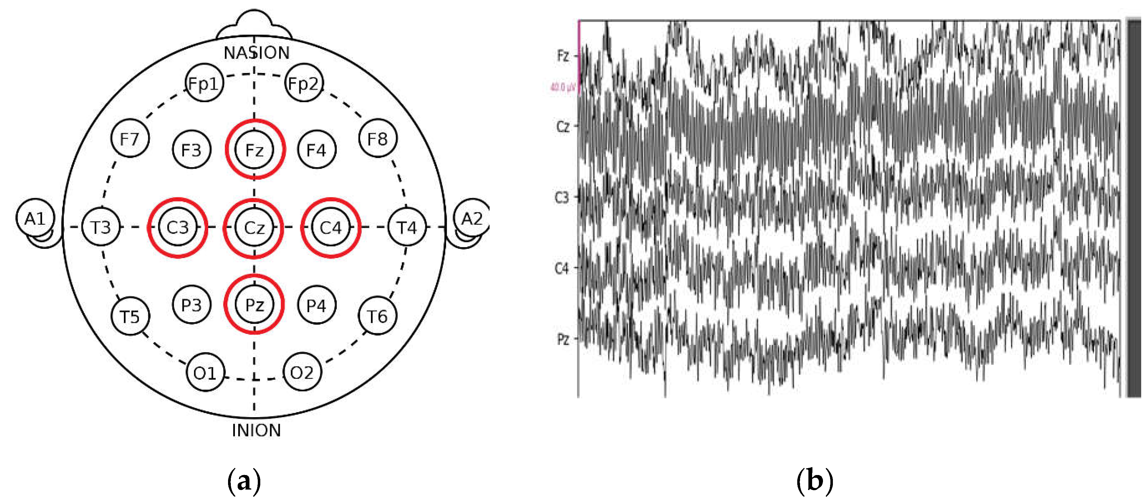
DROZY provides recordings for five EEG leads (Fz, Cz, C3, C4, and Pz) in the EDF format, with a sample rate equal to 512 Hz. The principle of this database is to study the states of alertness of 14 healthy subjects devoid of drug problems, alcohol consumption, or sleep disorders during a Psychomotor Vigilance Test (PVT). The data collection protocol requires subjects to repeat the PVT three times over two days without sleeping (totaling 28.30 hours without sleep) in order to identify the level of vigilance of each subject in the various periods of the day (morning, noon, night).
After each PVT, subjects are asked to specify their level of alertness using the Karolinska Sleepiness Scale (KSS). KSS is a scale composed of nine states of vigilance (1 = extremely alert, 2 = very alert, 3 = alert, 4 = sufficiently alert, 5 = neither alert nor drowsiness, 6 = some signs of drowsiness, 7 = drowsiness but no effort to remain vigilant, 8 = drowsiness with little effort to remain vigilant, 9 = very sleepy). In this work, we are interested in detecting drowsiness, without specifying the level of vigilance. For this reason, levels 1, 2, 3, 4, and 5 are considered stage 0 (alert), and levels 6, 7, 8, and 9 are considered stage 1 (drowsy).
Figure 2.
DROZY EEG signals [50]: (a) Location of EEG electrodes according to international system 10-20 (Fz, Cz, C3, C4, Pz); (b) EEG raw.
Figure 2.
DROZY EEG signals [50]: (a) Location of EEG electrodes according to international system 10-20 (Fz, Cz, C3, C4, Pz); (b) EEG raw.
4. Materials and Methods
The proposed approach is a binary method designed to distinguish between two states of vigilance: wakefulness and drowsiness.
The first step is to filter the raw EEG via a FIR bandpass filter ([0.1; 30] Hz) to eliminate high frequencies irrelevant to the study of drowsiness, such as artifacts from electrical and electromagnetic interference. Subsequently, the filtered EEG signals are segmented into segments of two sizes, 30 and 10 seconds respectively, to determine the most effective duration for drowsiness detection. These EEG segments are then normalized using the z-score method before feature extraction.
Feature extraction involves capturing both statistical time characteristics and frequency features, using the Welch method to compute the RPSD of each frequency wave. Time-Frequency (TF) analysis is conducted using the DWT, providing coefficients that depict the frequency evolution of the EEG signal over time. Thereafter, we will apply a standardization operation on all the characteristics. Subsequently, the Recursive Feature Elimination Cross-Validation (RFECV) is used to select the most significant features.
The selected features are fed into various classification algorithms to determine their class and accuracy of the different ML classification models tested in both intra and inter modes Figure 3 shows the general scheme of the proposed method. As detailed in the results section, all evaluations are performed using Python version 3 on an Intel(R) Core ™i5-8th Gen processor of 1.70 GHz with 8 GB of RAM.
4.1. EEG Features
- Statistical characteristics over time
The extraction of statistical features of EEG signals [11] does not focus on dynamic analysis, unlike signal processing-based methods. Nevertheless, it offers valuable features for drowsiness detection without necessitating extensive knowledge of EEG patterns associated to the states of vigilance of individuals. In this work, the temporal statistical features used are respectively Standard deviation (STD), asymmetry (Skew), and Kurtosis (Kurt). Equations (1), (2), and (3) represent each feature, denoted as follows:
Xi represents the data, which in our case is EEG data, i = 1…N, where N is the number of samples, and mean is the mean.
- Relative power spectral density
The PSD [26,27] algorithm quantifies the power distribution of EEG signals across predefined frequency bands, typically ranging from 0.1 to 30 Hz for hypovigilance studies.
Common methods for PSD calculation include Welch, FFT, and Brug. Among these, the Welch method has been identified as the most efficient for analyzing reduced vigilance. Consequently, we will utilize the Welch method in our study. If we denote P as the average power of a signal x(t), then the total power over a duration T is calculated as shown in equation (4):
If the output of the Welch transformation is denoted as (w), representing the frequency content of the x(t) signal, the PSD can be calculated as follows (5):
denotes the average or expected value operator. Here, it signifies the average of the squared magnitude of the inner product between vectors x and w. In essence, represents the averaged squared magnitude of the projection of one vector onto another. This notation is common in signal processing and statistics, particularly when dealing with stochastic processes or random variables.
The drowsiness detection via PSD can encounter significant variability among individuals and even with the same individual over time. This issue heightens inter-subject variability and hinders the development of a generalized drowsiness detection system. To avoid this problem and create a general system capable of consistent efficiency and accuracy across different individuals, we will use The Relative Power Spectrum Density (RPSD) [26]. The RPSD represents the ratio of the PSD within the frequency Band Of Interest (BOI) to the PSD across the entire frequency spectrum. The RPSD can be calculated as follows (6):
- Discrete Wavelet Transformation
The correlation between EEG signals and the wavelet function across different time intervals can be represented by the DWT coefficient. Moreover, DWT coefficients provide valuable information on the transient behavior of EEG signals.
For all these reasons, we will use the DWT coefficients as features for vigilance decline detection. Our approach employs the Daubechies wavelet function (“db4”) for coefficient extraction, as this wavelet function captures relevant information related to drowsiness [40]. The DWT coefficients are calculated as shown in (7),(8):
The two variables l and n represent the wavelet scale and the translation variables. The choice of two variables, l and n, is made on a dyadic scale, as explained in equation (8), to ensure orthogonality so that the original signal reconstruction can be performed. Variable l offers signal analysis in the frequency domain: The high-frequency components of the original signal are represented by the compressed version of the wavelet function, and the components of the low frequency are represented by the stretched version of the wavelet function. Variable n provides temporal analysis of the signal.
The output of DWT will consist of two types of coefficients as shown in Figure 4: Detail coefficients (cD) and Approximation coefficients (cA). These coefficients represent details (capturing high-frequency components) and approximation (capturing low-frequency components), respectively. For each coefficient type, energy (9), entropy (10), standard deviation (11), and mean (12) will be calculated.
4.2. Feature Selection
RFECV represents a sophisticated approach to feature selection that merges the advantages of RFE [17] with cross-validation. This technique is especially useful when the goal is to choose the most relevant features for a ML model, while simultaneously estimating the optimal number of features to consider. RFECV is distinguished by its focus on automating this complex process and determining the ideal number of features to maximize model performance.
The RFECV [51] starts with an initial ML model and a complete set of features. After evaluating the contribution of each feature to model performance. It iteratively removes the least important ones. Following each elimination, cross-validation is used to assess the performance of the model. This process repeats until a predefined criterion, such as model accuracy, reaches an optimum or an optimal number of features is identified.
Cross-validation is crucial in the RFECV process as it ensures that feature selection is robust and generalizable. By partitioning the data into subsets, cross-validation evaluates the performance of the model across various datasets, thus reducing the risk of over-fitting. Figure 5 explains how RFECV works.
5. Final Data, Classification and Validation
5.1. Final Data
In this work, we will assess the efficacy of our approach in two modes of drowsiness investigation: intra and inter modes. The objective is to mitigate EEG signal variability and validate the generalizability of our system.
For each DROZY subject [50], three EEG recordings are accessible, where each recording scored uses the KSS scale. This stage aims to extract the features of vigilance records and label them as stage '0' after the normalization operation. To ensure binary classification, we use the same process for the drowsiness state and label the features as stage '1'. DROZY EEG signals are recorded with five electrodes, and 16 features are extracted for each electrode, resulting in a total of 80 features.
The initial phase involves evaluating the performance of the approach in the intra mode, conducted separately for each subject. The input data were partitioned into 70% for training and 30% for testing purposes. The overall accuracy of the classification is determined by averaging the results across all subjects as shown in Figure 6.
The second phase aims to improve the ability to address inter-individual disparities. We test four data distribution protocols to identify the most effective one for training the ML model to accurately detect drowsiness across different subjects. Table 1 displays the distribution of subjects for each protocol:
- Cross-subject: In this data distribution mode, we employ a single subject as the test case in each iteration to evaluate the performance of the ML model trained on the remaining data.
- Combined-subject: In this mode, the characteristics of all subjects are combined and divided into 70% for training and 30% for validation games.
5.2. Classification Algorithms
After extracting the feature vectors and implementing the feature importance selection, we will move on to classify the vigilance states into two states (Awake, and Drowsy). There are several classifiers for automatic identification of drowsiness. ML models that can detect drowsiness and support the nonlinearity of EEG signals are listed below.
- SVM
SVMs [52] are ML algorithms used in machine learning to solve problems of classification, regression, or anomaly detection.
The main goal of the SVM is to separate data into classes using as simple a border as possible. The distance between the data sets and the boundary between them must be maximum. This distance is called margin, so SVMs are called wide margin separators. The data closest to the border is called carrier vectors. The SVM function is calculated as follows (13):
Where (xi,yi) represents the training dataset, which is 1<i<N. x represents the characteristic vector extracted from the EEG signals, y indicates the corresponding vigilance status labels, and N is the number of data. Moreover, K is the kernel function of the SVM, Si is the vector support, are the weights, and b is the bias.
- KNN
KNN [53] is an ML algorithm that is simply and easily used to implement supervised learning algorithms that can be utilized for solving classification and regression problems.
The purpose of the KNN algorithm is to use a database in which the data points are separated into several distinct classes to predict the classification of a new sample point.
KNN is one of the simplest supervised ML algorithms that applies the following steps on the database to predict the new point class:
Step 1 : Select the number K of neighbors.
Step 2 : Calculate the distance between the unclassified point and the other points.
Step 3 : Take the nearest K according to the calculated distance.
Step 4 : Count the number of points belonging to each category among these K neighbors.
Step 5 : Assign the new point to the most present category allowed by these K neighbors.
Most KNN classifiers use the Euclidean metric to measure differences between examples represented as vector inputs. Euclidean distance is defined as (14):
- Naive Bayes
The Naive Bayes (NB) classification represents a kind of simple probabilistic classification based on the Bayes theorem [54]. Simply put, the Bayesian model is a classifier that assumes that the existence of a characteristic for a class is independent of the existence of other characteristics. NB classifiers work in the context of supervised learning. Classifiers have several advantages such as their ability to support little training data to make the estimation of parameters necessary for classification.
- Decision tree
A Decision Tree (DT) is one of the most widely used decision tools. This tool provides a diagram of a tree that represents a set of choices [55]. The ends of the branches of the trees, also known as the leaves of the tree, show the different possible decisions that are made according to the decisions made at each stage. Several areas, such as safety and medicine use DT for their advantages in terms of readability and speed of execution. It is also a representation that can be calculated automatically by supervised ML algorithms.
- MLP
An MLP [56] represents a kind of direct-acting Artificial Neural Network (ANN). MLPs are typically composed of three layers of nodes which are an input layer, a hidden layer, and an output layer, respectively. Each input node represents a neuron that uses a non-linear activation function. The MLP uses a supervised learning technique based on a string rule called the reverse propagation mode or the automatic reverse differentiation to establish training. Its multiple layers and nonlinear activation distinguish the MLP from a linear perceptron; it can distinguish data that are not linearly separable.
5.3. Evaluation Metrics
For the evaluation of the performance of the different classifiers, we will use the binary confusion matrix presented in Figure 7.
True Positive (TP): prediction of drowsiness when the actual state is drowsiness.
False Positive (FP): prediction of drowsiness when the real state is alertness.
True Negative (TN): prediction of alertness when the real state is alertness.
False Negative (FN): prediction of alertness when the real state is drowsiness.
The performance measures used in this work are Accuracy (A), Precision (P), Sensitivity (S), and F1-score (F1). Equations (15), (16), (17) and (18) respectively represent the equation for each performance indicator:
6. Results and Discussion
In this part, we will present the results in both intra and inter-modes.
6.1. Intra Mode
This section showcases the outcomes of detection in the intra mode to emphasize the accuracy of this method in detecting drowsiness for every individual separately from others. Our initial step is to examine how accurate this approach is with two different segment sizes, 30 and 10 seconds, to determine which one is most effective for detecting drowsiness. The accuracy of the different classifiers for both sizes is shown in Figure 8.
By visualizing the graph, we can say that the 10-second segments offer more precision in detecting drowsiness. The following table represents the classification results of different classifiers with 10-second segments.

Table 2.
Different classifiers accuracy with 10-second segments in the intra mode.
| Subjects | NB (accuracy %) |
KNN (accuracy %) |
DT (accuracy %) |
MLP (accuracy %) |
SVM (accuracy %) |
|---|---|---|---|---|---|
| Subject 1 | 78 | 81.9 | 82 | 94 | 95.8 |
| Subject 2 | 81 | 86 | 81 | 94.4 | 98 |
| Subject 3 | 87.5 | 94.4 | 88.8 | 99 | 98.6 |
| Subject 4 | 99.6 | 98.95 | 95.8 | 99.9 | 99 |
| Subject 5 | 84.72 | 87.5 | 95.6 | 97.2 | 97.5 |
| Subject 6 | 94 | 94.4 | 94 | 98.6 | 98.8 |
| Subject 7 | 93 | 86 | 84.7 | 94 | 94 |
| Overall | 88.26 | 89.87 | 88.84 | 96.72 | 97.38 |
On the other hand, the use of five electrodes does not represent an adaptable method for certain real conditions. Several approaches use a single electrode to detect decreased alertness. However, it is not accurate because the system no longer works if the electrode turns off or comes into bad contact with the scalp.
To avoid this problem and create an adaptable system with the conditions of the embedded systems (energy consumption, size, etc.), we move on to determine the two most efficient deviations to minimize the number of electrodes and maintain accuracy. Table 3 represents the performance for each classifier with each deviation.
From these results, it can be inferred that C3 and C4 are the two most accurate leads for detecting drowsiness. To adapt to the embedded system's requirements and make the system more adaptable to real-life conditions, we reduce the number of electrodes in our approach to two (C3 and C4) for the remainder of the work.
On the other hand, the importance of features varies from one subject to another. To avoid this problem and to improve the accuracy of the approach we use a method of feature importance selection to reduce the number of features and keep only the most useful ones at the level of drowsiness detection for each individual (Figure 9). RFECV is the selection method employed in this work.
RFECV provides us with the most important features for each subject and eliminates the least important. Table 4 represents the number of most important characteristics for each subject.
Figure 10.
The number of features selected by RFECV with SVM.
The research shows that the SVM with the Radial Basis Function (RBF) kernel is the most exact classifier for detecting drowsiness in the intra mode, with just two C3-C4 derivations and seven features picked by RFECV, with an overall accuracy of 99.85%.
6.2. Inter Mode
In this section, we will work with three temporal characteristics, five frequencies, and eight TFs, which gives us 16 characteristics per electrode. For two electrodes, we have 2*16 = 32 characteristics. Our work consists in evaluating the performance of our approach with two EEG derivations in four different data distribution protocols. Moreover, comparing the results with the intra-mode to specify the most effective data distribution protocol to train a more generalist model that can eliminate and overcome the problem of EEG variability between subjects.
Subsequently, we move on to the use of the RFECV to select the most important features and eliminate the less decisive features in connection with the detection of drowsiness. This feature selection method will help us decrease the features on the one hand and increase the system accuracy on the other hand.
As in the intra mode, we start by identifying the two electrodes that have the highest accuracy in the inter mode for later use (Figure 11).
Table 5, Table 6, Table 7, Table 8 and Table 9 represent the classification results for the original data with only two EEG leads (C3 and C4) without the use of the feature significance selection method for four data distribution protocols.
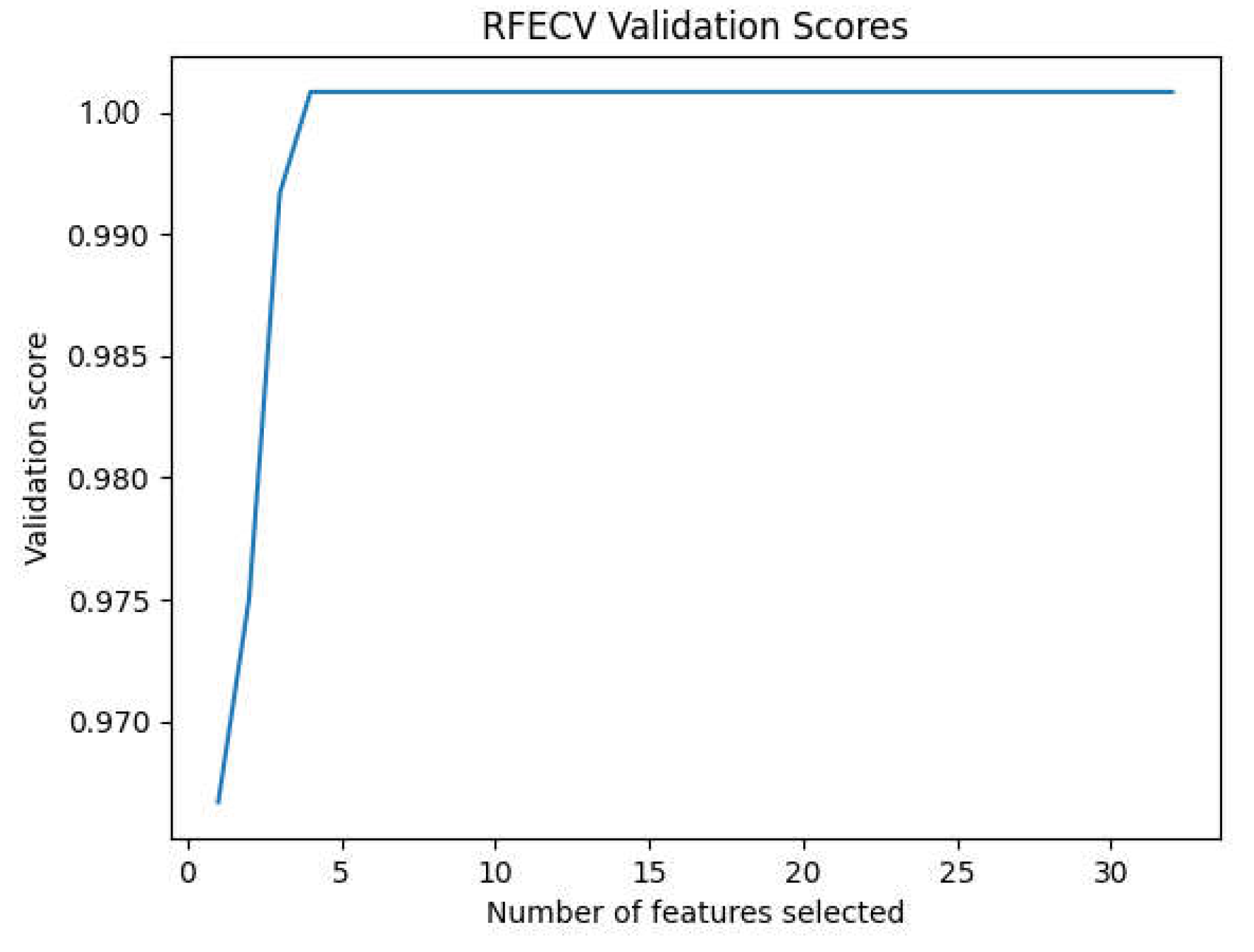
Based on the results, we can see that the C3-C4 represents the most accurate leads in the inter mode, but we can also see that the accuracy of the approach considerably decreases. For this reason, the next phase is to use a significant feature selection method known as RFECV to select the most important features concerning drowsiness to increase the accuracy of the approach. Figure 12 shows the evolution of the precision of the approach according to the number of characteristics selected by RFECV.
The maximum accuracy obtained after the use of the RFECV in the inter mode is that of MLP with a value of 96.4% with protocol P4 as shown in Table 10 with a number of characteristics selected by RFECV equal to nine features. As a result, we can see that the accuracy of the approach considerably decreases with the reduction in the number of tracks as well as in the features compared to the results of the intra-subject mode. On the other hand, we can see that the approach can overcome EEG variability with a high accuracy rate.
6.3. Comparison of RFECV with Other Feature Selection Methods
In this part, we compare the performance of the approach using other feature selection methods, k-PCA and PCA, to clarify the effect of the selection method on the performance of the approach. Figure 13 represents the results of the classification of the selection method proposed in this work with k-PCA and PCA with the data distribution of protocol P4.
Based on the results, we can clearly see that the RFECV is more effective as a feature selection method for drowsiness detection in comparison with k-PCA and PCA.
6.4. Discussion
The variability observed in EEG signals, both in individuals and in different subjects, poses significant obstacles to the advancement and practical application of drowsiness detection systems. The critical step in selecting appropriate characteristics to identify declines in vigilance is complicated by the considerations of the variability of EEG between subjects and adaptability to real conditions. In this work, alternative techniques such as statistical analysis, the Welch method, and DWT are used to extract the temporal, frequency and TF characteristics of the EEG signals. Subsequently, feature selection is applied to mitigate interpersonal variability while maintaining detection accuracy, resulting in an impressive accuracy rate of 96.4%. The integration of two EEG channels enriches the versatility of the system in various environments, making it better suited for real-time deployment. In addition, the simplification of the system through the removal of redundant features increases the efficiency and adaptability of the classification, resulting in an improvement in accuracy up to 94.8% when using all features (80 features), and an additional improvement to 96.4 when using only 9 features. Using the RFECV algorithm, classification accuracy is further improved to 96.4% while reducing system complexity by decreasing the number of features from 80 to 9. This study represents an important step towards the development of a drowsiness monitoring device based on EEG signals. Importantly, existing studies have explored EEG-based drowsiness detection. Moreover, we provide in Table 11 a comparative analysis of our approach versus common methodologies.
7. Conclusion
Decreased alertness, especially passive wakefulness (drowsiness), is a very dangerous condition in areas such as transportation, industry, and medicine. In this work, we have proposed an approach to drowsiness detection based on EEG features coming from two EEG leads (C3, C4). The suggested system uses the Welch method, the EEG statistical characteristics and the DWT to extract the different EEG characteristics in time, frequency and TF domains, respectively. The RFE technique has been used as a selection method to keep the most important features to ensure more accurate and generic drowsiness detection. The different ML models have been utilized to differentiate two states of vigilance (awake, drowsy). The proposed system is capable of detecting drowsiness with accuracy of 99.85% and 96.4%, respectively in intra and inter modes. The strengths of the suggested approach are represented by their ability to overcome the inter-subject problem and they offer a more generalized system with a high accuracy rate. In addition, the proposed drowsiness detection system uses a limited number of EEG electrodes, which makes it more adaptable to real-life conditions. As a perspective, we aim to incorporate facial expressions as well as other physiological signals, such as EOG and ECG, with the EEG signal to strengthen the reliability of the approach. In addition, the implementation of this approach on a programmable platform for the creation of an embedded drowsiness detection system represents a future topic.
Funding
This research received no external funding.
Institutional Review Board Statement
Not applicable.
Informed Consent Statement
Not applicable.
Data Availability Statement
Not applicable.
References
- VAN SCHIE, Mojca KM, LAMMERS, Gert Jan, FRONCZEK, Rolf, et al. Vigilance: discussion of related concepts and proposal for a definition. Sleep Medicine, 2021, vol. 83, p. 175-181. [CrossRef]
- GIBBINGS, A., RAY, L. B., BERBERIAN, N., et al. EEG and behavioural correlates of mild sleep deprivation and vigilance. Clinical Neurophysiology, 2021, vol. 132, no 1, p. 45-55.
- SLATER, Jeremy D. A definition of drowsiness: One purpose for sleep?. Medical Hypotheses, 2008, vol. 71, no 5, p. 641-644.
- WU, Yingzhang, ZHANG, Jie, LI, Wenbo, et al. Towards Human-Vehicle Interaction: Driving Risk Analysis Under Different Driver Vigilance States and Driving Risk Detection Method. Automotive Innovation, 2023, vol. 6, no 1, p. 32-47.
- WANG, Hanyu, CHEN, Dengkai, HUANG, Yuexin, et al. Assessment of vigilance level during work: fitting a hidden Markov model to heart rate variability. Brain sciences, 2023, vol. 13, no 4, p. 638.
- JING, Meng-Juan, LI, Hao, LI, Chun-Peng, et al. The Association between Working Hours with Vigilance and Executive Function of Intensive Care Unit Nurses. Journal of Nursing Management, 2023, vol. 2023.
- JAGANNATHAN, Sridhar R., BAREHAM, Corinne A., et BEKINSCHTEIN, Tristan A. Decreasing alertness modulates perceptual decision-making. Journal of neuroscience, 2022, vol. 42, no 3, p. 454-473.
- ALBADAWI, Yaman, TAKRURI, Maen, et AWAD, Mohammed. A review of recent developments in driver drowsiness detection systems. Sensors, 2022, vol. 22, no 5, p. 2069.
- ALBADAWI, Yaman, ALREDHAEI, Aneesa, et TAKRURI, Maen. Real-time machine learning-based driver drowsiness detection using visual features. Journal of imaging, 2023, vol. 9, no 5, p. 91.
- FRANÇOIS, Clémentine. Development and validation of algorithms for automatic and real-time characterization of drowsiness. 2018.
- LI, Gang et CHUNG, Wan-Young. Electroencephalogram-based approaches for driver drowsiness detection and management: A review. Sensors, 2022, vol. 22, no 3, p. 1100.
- FOUAD, Islam A. A robust and efficient EEG-based drowsiness detection system using different machine learning algorithms. Ain Shams engineering journal, 2023, vol. 14, no 3, p. 101895.
- BAJAJ, Jaspreet Singh, KUMAR, Naveen, KAUSHAL, Rajesh Kumar, et al. System and method for driver drowsiness detection using behavioral and sensor-based physiological measures. Sensors, 2023, vol. 23, no 3, p. 1292. [CrossRef]
- NAIK, Ganesh R. et KUMAR, Dinesh K. An overview of independent component analysis and its applications. Informatica, 2011, vol. 35, no 1.
- BHARADIYA, Jasmin Praful. A tutorial on principal component analysis for dimensionality reduction in machine learning. International Journal of Innovative Science and Research Technology, 2023, vol. 8, no 5, p. 2028-2032.
- SCHÖLKOPF, Bernhard, SMOLA, Alexander, et MÜLLER, Klaus-Robert. Kernel principal component analysis. In : International conference on artificial neural networks. Berlin, Heidelberg : Springer Berlin Heidelberg, 1997. p. 583-588.
- ZENG, Xiangyan, CHEN, Yen-Wei, et TAO, Caixia. Feature selection using recursive feature elimination for handwritten digit recognition. In : 2009 Fifth International Conference on Intelligent Information Hiding and Multimedia Signal Processing. IEEE, 2009. p. 1205-1208.
- KILMEN, Sevilay et BULUT, Okan. Scale abbreviation with recursive feature elimination and genetic algorithms: An illustration with the test emotions questionnaire. Information, 2023, vol. 14, no 2, p. 63. [CrossRef]
- DOGAN, Sengul, TUNCER, Ilknur, BAYGIN, Mehmet, et al. A new hand-modeled learning framework for driving fatigue detection using EEG signals. Neural Computing and Applications, 2023, vol. 35, no 20, p. 14837-14854. [CrossRef]
- WANG, Yao, HUANG, Yuecheng, GU, Botao, et al. Identifying mental fatigue of construction workers using EEG and deep learning. Automation in Construction, 2023, vol. 151, p. 104887. [CrossRef]
- GANGADHARAN, Sagila et VINOD, A. P. Drowsiness detection using portable wireless EEG. Computer Methods and Programs in Biomedicine, 2022, vol. 214, p. 106535.
- FOUAD, Islam A. A robust and efficient EEG-based drowsiness detection system using different machine learning algorithms. Ain Shams engineering journal, 2023, vol. 14, no 3, p. 101895.
- BENCSIK, Blanka, REMÉNYI, István, SZEMENYEI, Márton, et al. Designing an embedded feature selection algorithm for a drowsiness detector model based on electroencephalogram data. Sensors, 2023, vol. 23, no 4, p. 1874.
- RAMOS, Plínio MS, MAIOR, Caio BS, MOURA, Márcio C., et al. Automatic drowsiness detection for safety-critical operations using ensemble models and EEG signals. Process Safety and Environmental Protection, 2022, vol. 164, p. 566-581. [CrossRef]
- KRISHNAN, Pranesh, YAACOB, Sazali, KRISHNAN, Annapoorni Pranesh, et al. EEG based Drowsiness Detection using Relative Band Power and Short-time Fourier Transform. J. Robotics Netw. Artif. Life, 2020, vol. 7, no 3, p. 147-151.
- YAACOB, Sazali, AFFANDI, Nur Afrina Izzati, KRISHNAN, Pranesh, et al. Drowsiness detection using EEG and ECG signals. In : 2020 IEEE 2nd International Conference on Artificial Intelligence in Engineering and Technology (IICAIET). IEEE, 2020. p. 1-5.
- ABIDI, Afef, BEN KHALIFA, Khaled, BEN CHEIKH, Ridha, et al. Automatic detection of drowsiness in EEG records based on machine learning approaches. Neural Processing Letters, 2022, vol. 54, no 6, p. 5225-5249.
- SALEEM, Adil Ali, SIDDIQUI, Hafeez Ur Rehman, RAZA, Muhammad Amjad, et al. A systematic review of physiological signals based driver drowsiness detection systems. Cognitive Neurodynamics, 2023, vol. 17, no 5, p. 1229-1259.
- JIANG, Xiao, BIAN, Gui-Bin, et TIAN, Zean. Removal of artifacts from EEG signals: a review. Sensors, 2019, vol. 19, no 5, p. 987.
- MUMTAZ, Wajid, RASHEED, Suleman, et IRFAN, Alina. Review of challenges associated with the EEG artifact removal methods. Biomedical Signal Processing and Control, 2021, vol. 68, p. 102741.
- ILLE, Nicole, NAKAO, Yoshiaki, YANO, Shumpei, et al. Ongoing EEG artifact correction using blind source separation. Clinical Neurophysiology, 2024, vol. 158, p. 149-158.
- YU, Junjie, LI, Chenyi, LOU, Kexin, et al. Embedding decomposition for artifacts removal in EEG signals. Journal of Neural Engineering, 2022, vol. 19, no 2, p. 026052.
- SEN, Dipanwita, MISHRA, Bhupati Bhusan, et PATTNAIK, Prasant Kumar. A review of the filtering techniques used in EEG signal processing. In : 2023 7th International Conference on Trends in Electronics and Informatics (ICOEI). IEEE, 2023. p. 270-277.
- STANCIN, Igor, CIFREK, Mario, et JOVIC, Alan. A review of EEG signal features and their application in driver drowsiness detection systems. Sensors, 2021, vol. 21, no 11, p. 3786.
- WANG, Yinghao, NAHON, Rémi, TARTAGLIONE, Enzo, et al. Optimized preprocessing and tiny ml for attention state classification. In : 2023 IEEE Statistical Signal Processing Workshop (SSP). IEEE, 2023. p. 695-699.
- ARIF, Saad, MUNAWAR, Saba, et ALI, Hashim. Driving drowsiness detection using spectral signatures of EEG-based neurophysiology. Frontiers in physiology, 2023, vol. 14, p. 1153268.
- ZAYED, Aymen, KHALIFA, Khaled Ben, BELHADJ, Nidhameddine, et al. Discrete Wavelet Transform Coefficients for Drowsiness Detection from EEG Signals. In : 2023 IEEE International Conference on Design, Test and Technology of Integrated Systems (DTTIS). IEEE, 2023. p. 1-6.
- ZHANG, Yuhao, GUO, Hanying, ZHOU, Yongjiang, et al. Recognising drivers’ mental fatigue based on EEG multi-dimensional feature selection and fusion. Biomedical Signal Processing and Control, 2023, vol. 79, p. 104237. [CrossRef]
- ESPINOSA, Ricardo, TALERO, Jesica, et WEINSTEIN, Alejandro. Effects of tau and sampling frequency on the regularity analysis of ecg and eeg signals using apen and sampen entropy estimators. Entropy, 2020, vol. 22, no 11, p. 1298.
- PENG, Yufan, WONG, Chi Man, WANG, Ze, et al. Fatigue detection in SSVEP-BCIs based on wavelet entropy of EEG. IEEE Access, 2021, vol. 9, p. 114905-114913.
- ZOU, Shuli, QIU, Taorong, HUANG, Peifan, et al. Constructing multi-scale entropy based on the empirical mode decomposition (EMD) and its application in recognizing driving fatigue. Journal of neuroscience methods, 2020, vol. 341, p. 108691.
- WANG, Fei, WAN, Yinxing, LI, Man, et al. Recent Advances in Fatigue Detection Algorithm Based on EEG. Intelligent Automation & Soft Computing, 2023, vol. 35, no 3.
- STANCIN, Igor, FRID, Nikolina, CIFREK, Mario, et al. EEG signal multichannel frequency-domain ratio indices for drowsiness detection based on multicriteria optimization. Sensors, 2021, vol. 21, no 20, p. 6932.
- SINGH, Anupreet Kaur et KRISHNAN, Sridhar. Trends in EEG signal feature extraction applications. Frontiers in Artificial Intelligence, 2023, vol. 5, p. 1072801.
- CHADDAD, Ahmad, WU, Yihang, KATEB, Reem, et al. Electroencephalography signal processing: A comprehensive review and analysis of methods and techniques. Sensors, 2023, vol. 23, no 14, p. 6434.
- BOMMERT, Andrea, SUN, Xudong, BISCHL, Bernd, et al. Benchmark for filter methods for feature selection in high-dimensional classification data. Computational Statistics & Data Analysis, 2020, vol. 143, p. 106839.
- MERA-GAONA, Maritza, LÓPEZ, Diego M., et VARGAS-CANAS, Rubiel. An ensemble feature selection approach to identify relevant features from EEG signals. Applied Sciences, 2021, vol. 11, no 15, p. 6983.
- DRUNGILAS, Darius, KURMIS, Mindaugas, LUKOSIUS, Zydrunas, et al. An adaptive method for inspecting illumination of color intensity in transparent polyethylene terephthalate preforms. IEEE Access, 2020, vol. 8, p. 83189-83198.
- EL-NABI, Samy Abd, EL-SHAFAI, Walid, EL-RABAIE, El-Sayed M., et al. Machine learning and deep learning techniques for driver fatigue and drowsiness detection: a review. Multimedia Tools and Applications, 2024, vol. 83, no 3, p. 9441-9477.
- MASSOZ, Quentin, LANGOHR, Thomas, FRANÇOIS, Clémentine, et al. The ULg multimodality drowsiness database (called DROZY) and examples of use. In : 2016 IEEE Winter Conference on Applications of Computer Vision (WACV). IEEE, 2016. p. 1-7.
- TRUJILLO, Leonardo, HERNANDEZ, Daniel E., RODRIGUEZ, Adrian, et al. Effects of feature reduction on emotion recogni-tion using EEG signals and machine learning. Expert Systems, p. e13577.
- ROY, Atin et CHAKRABORTY, Subrata. Support vector machine in structural reliability analysis: A review. Reliability Engi-neering & System Safety, 2023, vol. 233, p. 109126.
- ZHANG, Shichao. Challenges in KNN classification. IEEE Transactions on Knowledge and Data Engineering, 2021, vol. 34, no 10, p. 4663-4675.
- HASHIM, Keenan Ariqul, SIBARONI, Yuliant, et PRASETYOWATI, Sri Suryani. The Effectiveness of the Ensemble Naive Bayes in Analyzing Review Sentiment of the Lazada Application on Google Play. In : 2024 ASU International Conference in Emerging Technologies for Sustainability and Intelligent Systems (ICETSIS). IEEE, 2024. p. 1-5.
- ISSAH, Iddrisu, APPIAH, Obed, APPIAHENE, Peter, et al. A systematic review of the literature on machine learning applica-tion of determining the attributes influencing academic performance. Decision analytics journal, 2023, p. 100204.
- ABD-ELAZIEM, Ayman H. et SOLIMAN, Tamer HM. A Multi-Layer Perceptron (MLP) Neural Networks for Stellar Classifi-cation: A Review of Methods and Results‖. International Journal of Advances in Applied Computational Intelligence, vol. 3, no 10.54216.
- Cui, J. EEG Driver Drowsiness Dataset. 2021. Available online: https://figshare.com/articles/dataset/EEG_driver_drowsiness_ dataset/14273687/3 (accessed on 20 October 2022).
Figure 1.
Drowsiness detection with EEG signals general processing chain.
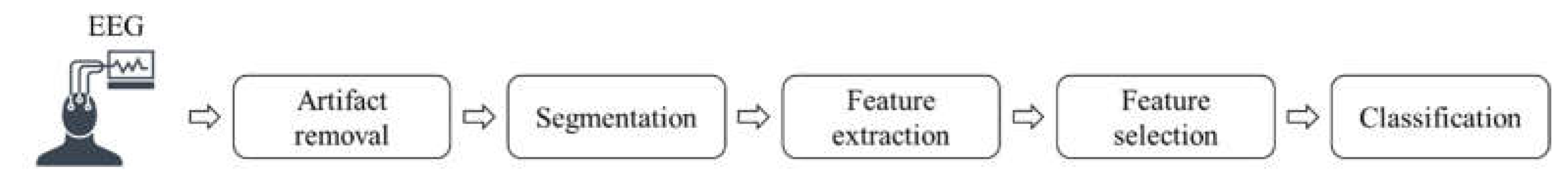
Figure 3.
The general scheme of the proposed method.
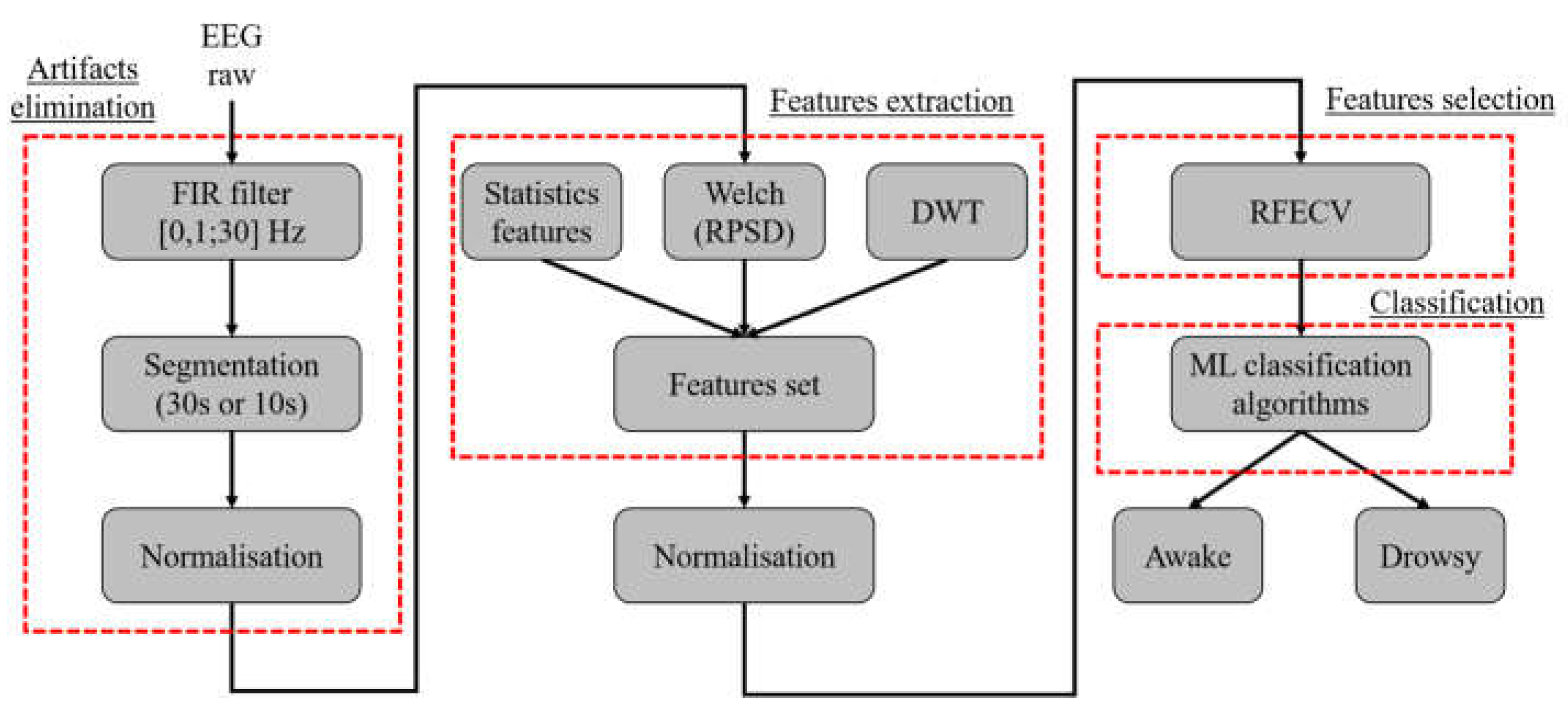
Figure 4.
EEG signal decomposition by the wavelet function [37].
Figure 4.
EEG signal decomposition by the wavelet function [37].
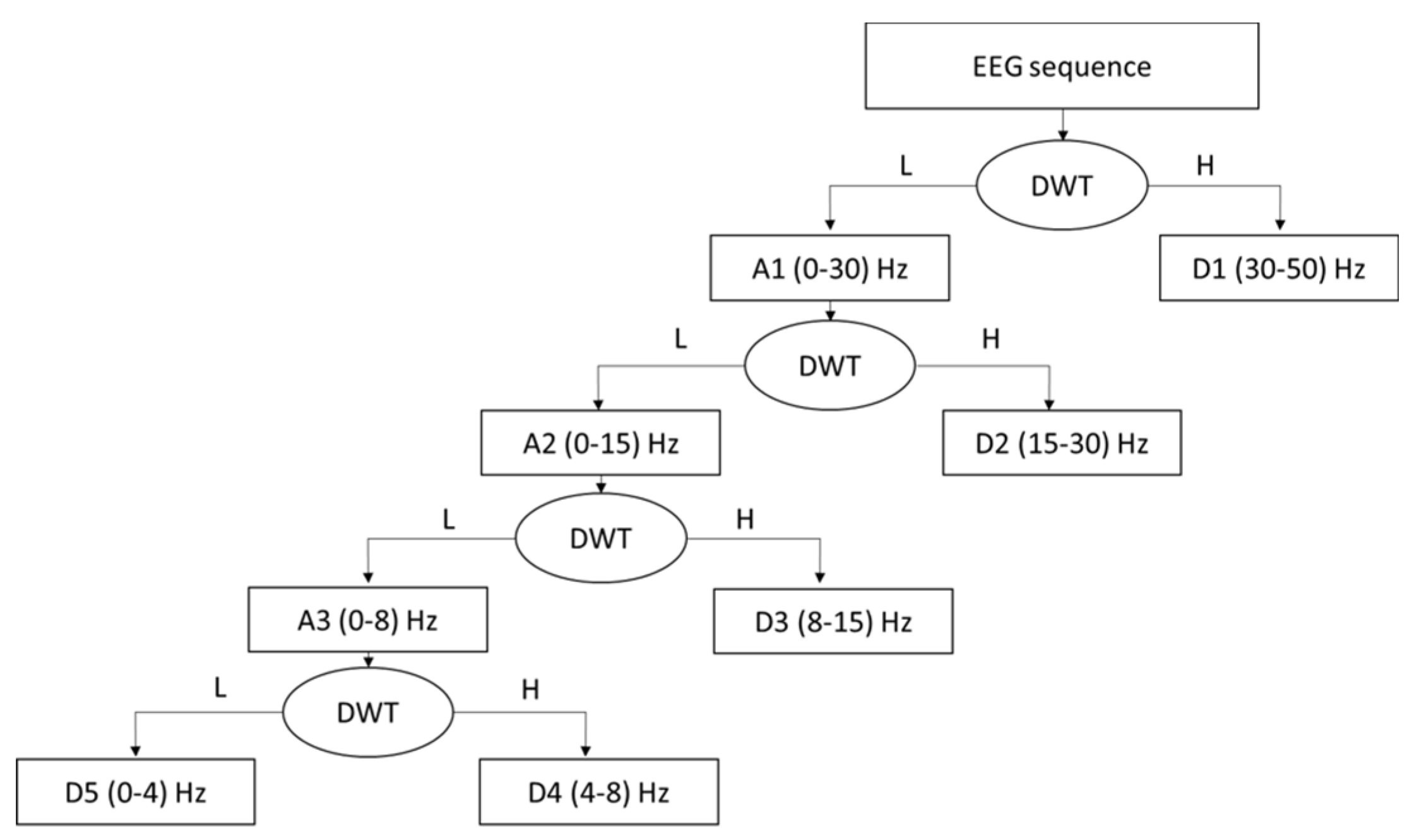
Figure 5.
Principle of operation of the RFECV.
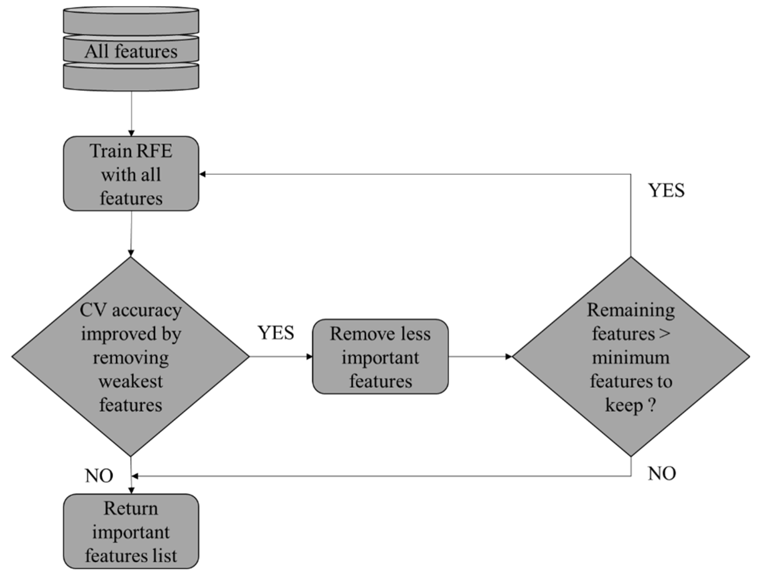
Figure 6.
Data distribution for the train and test sets in the intra mode.
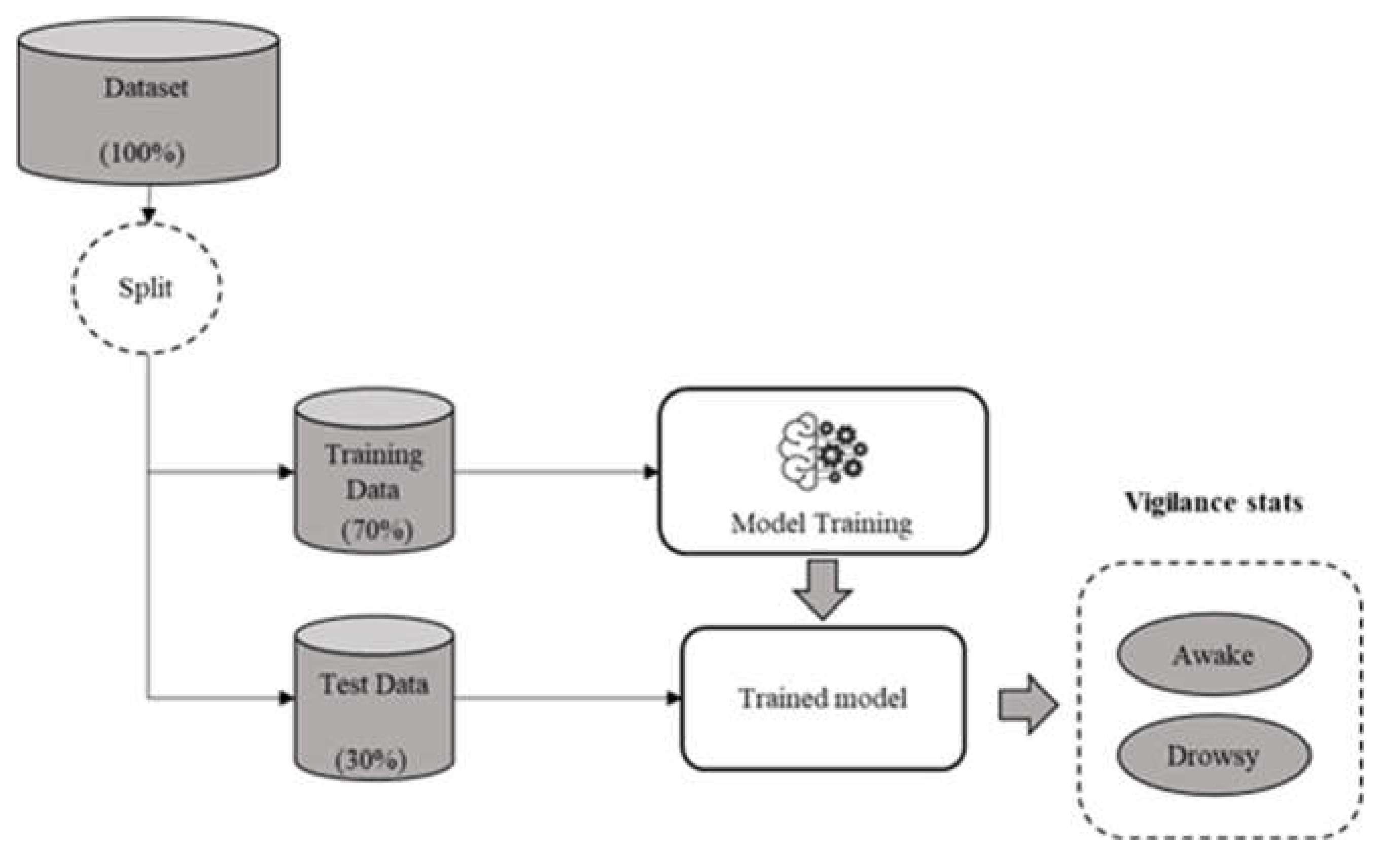
Figure 7.
Confusion matrix.

Figure 8.
Classification accuracy with 30 and 10 second segments.
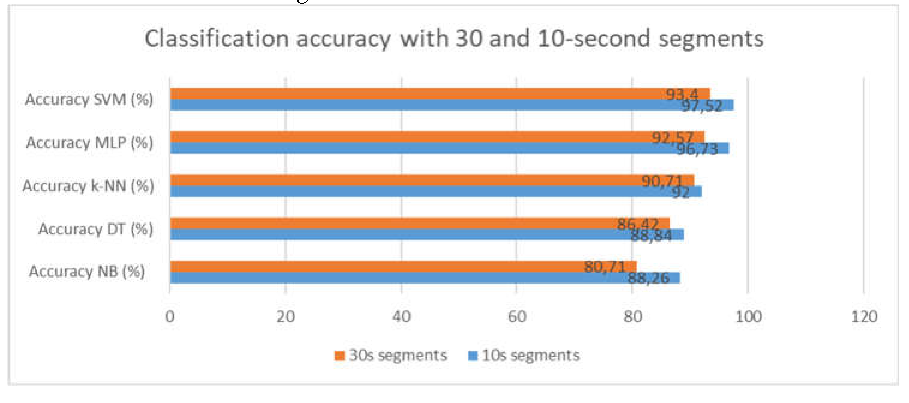
Figure 9.
Different classifiers accuracy after RFECV.
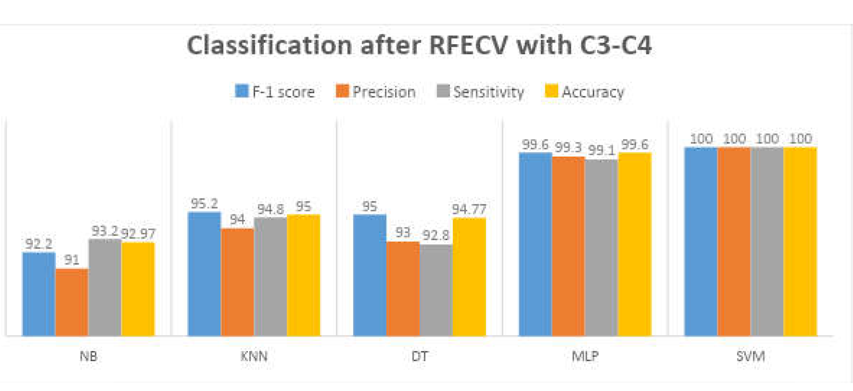
Figure 11.
Different classifiers accuracy with different EEG deviation in the inter mode.
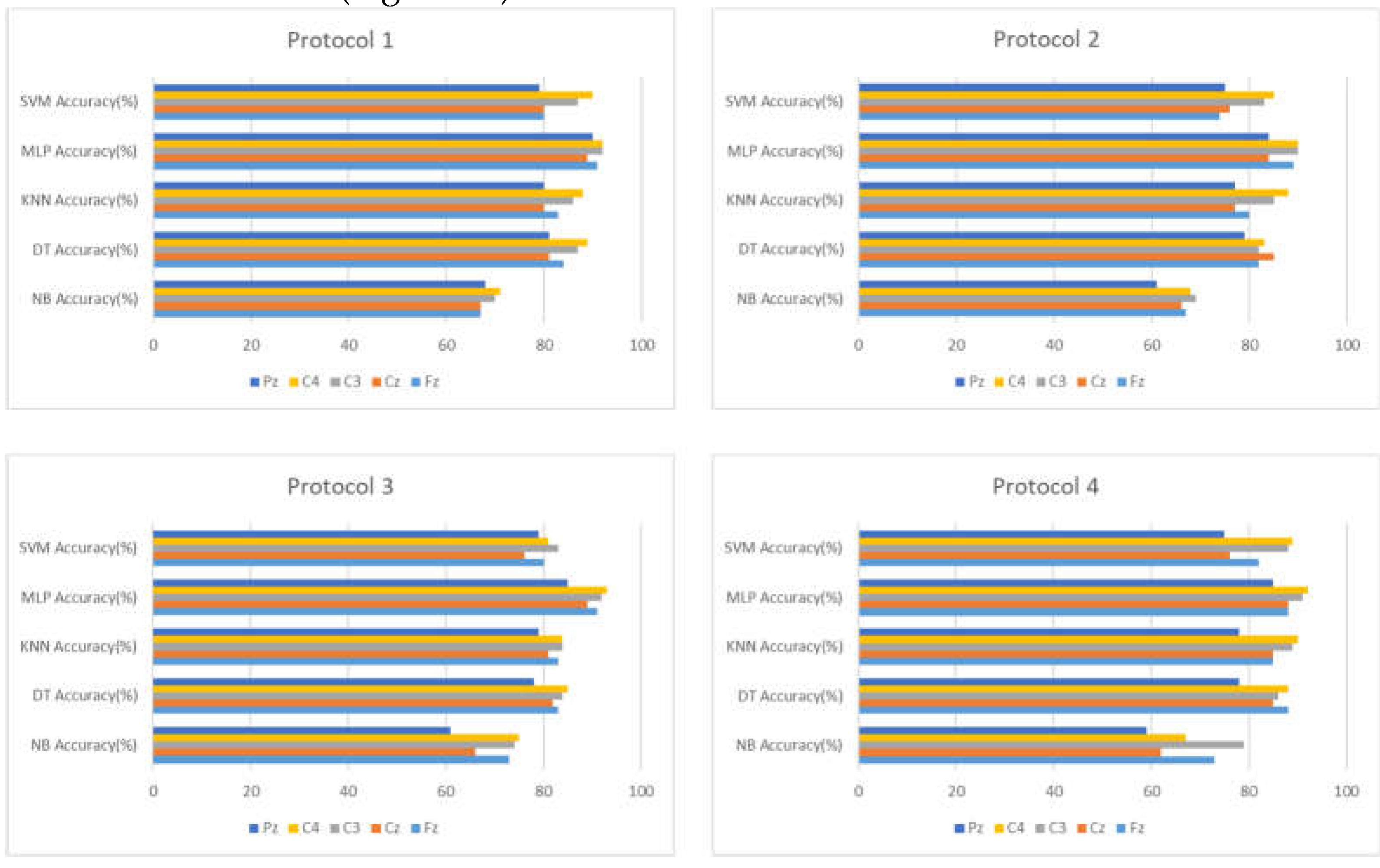
Figure 12.
The number of features selected by RFECV with MLP.
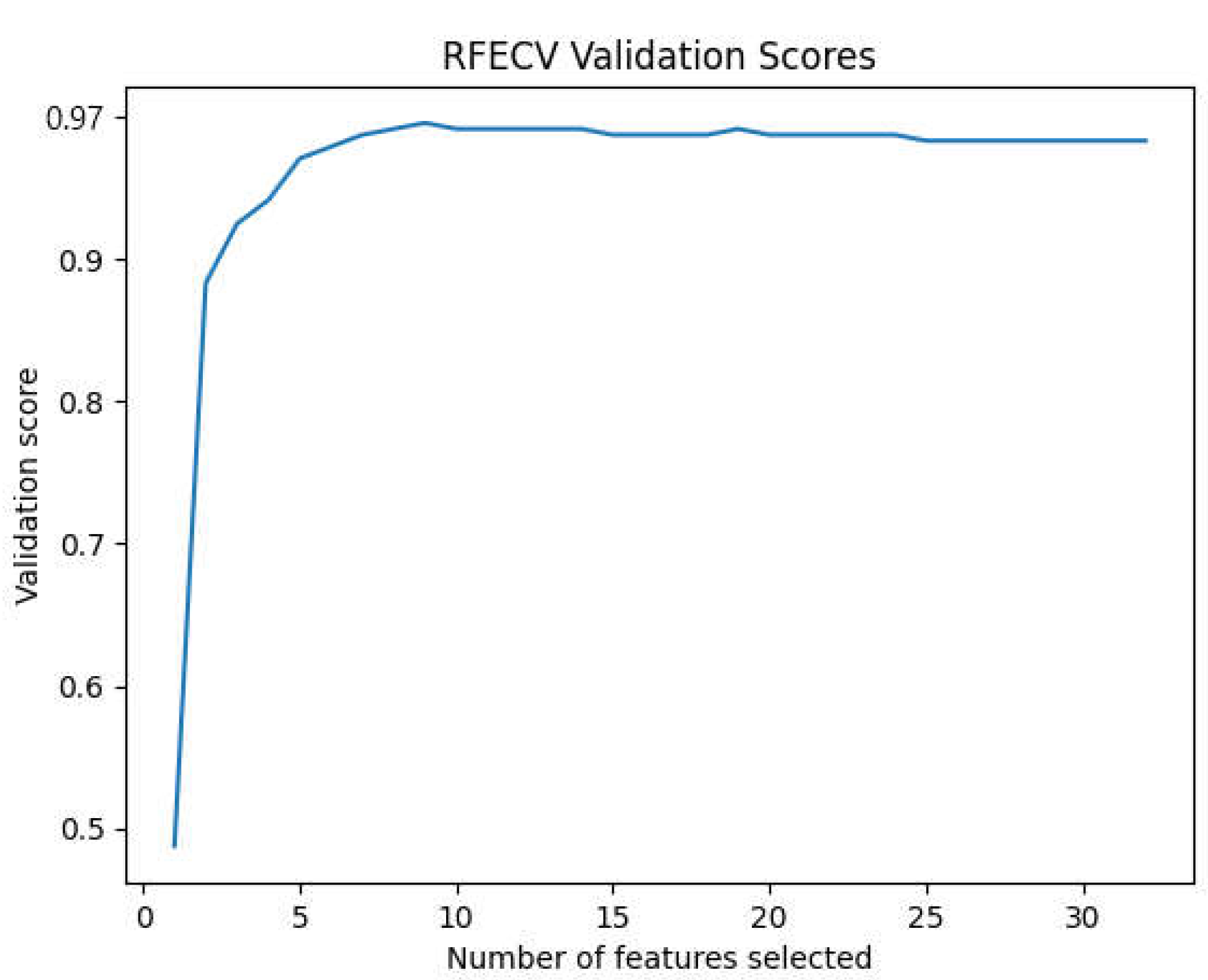
Figure 13.
The effect of the feature selection method on the accuracy of the approach.
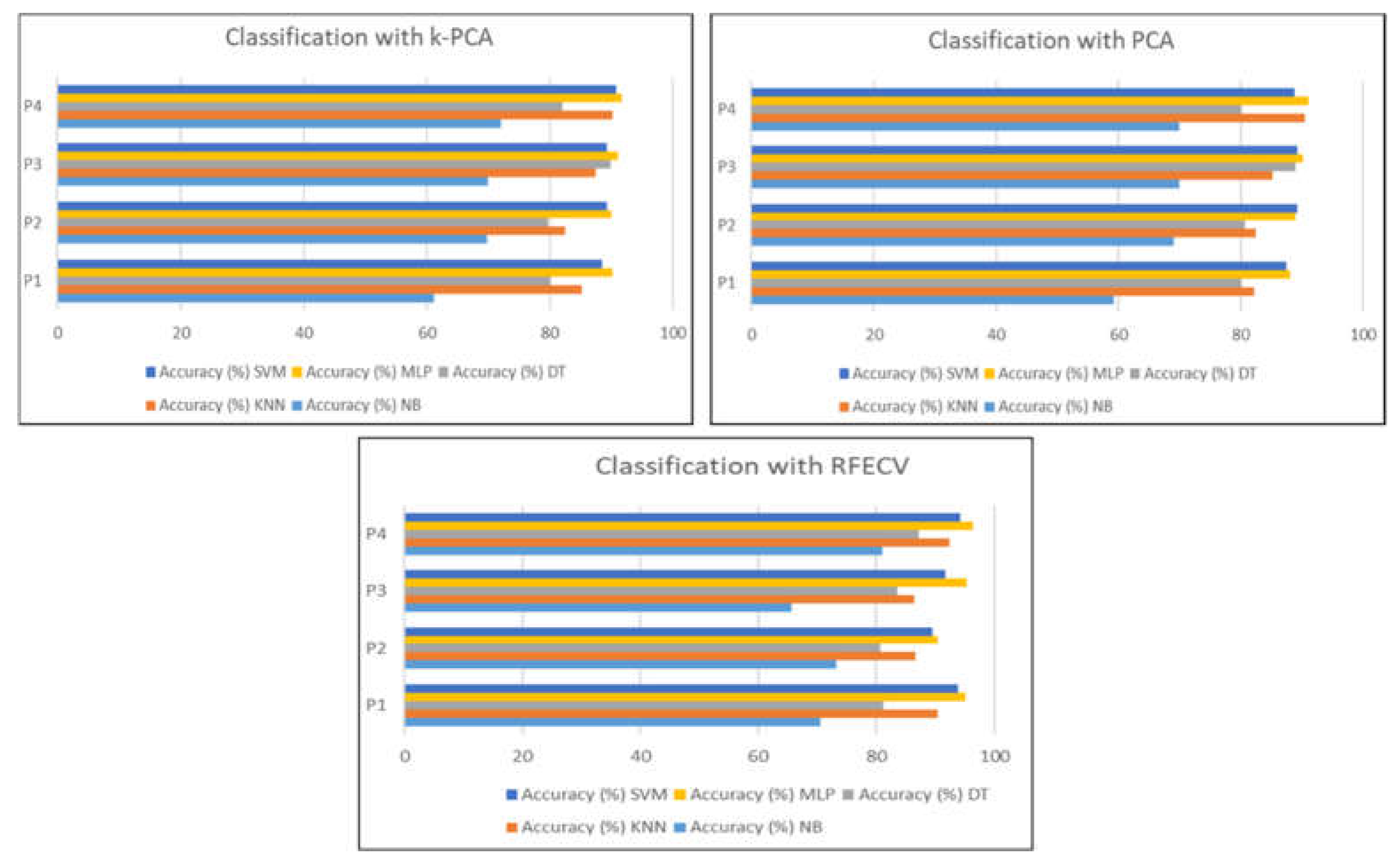
Table 1.
Data distribution protocols in the inter mode.
| Protocol names | Train data | Test data |
|---|---|---|
| P1 (combined-subject) | 70% of all features | 30% of all features |
| P2 (cross-subject) | Six subjects | One subject |
| P3 (cross-subject) | ||
| Five subjects | Two subjects | |
| P4 (cross-subject) | ||
| Four subjects | Three subjects |
Table 3.
Different classifiers accuracy with different EEG deviation in the intra mode.
| Derivation | NB (accuracy %) |
DT (accuracy %) |
KNN (accuracy %) |
MLP (accuracy %) |
SVM (accuracy %) |
|---|---|---|---|---|---|
| Fz | 82.8 | 67.52 | 79.92 | 71.2 | 75.5 |
| Cz | 83 | 79.2 | 79.1 | 75 | 83.5 |
| C3 | 87.8 | 88.1 | 85.6 | 90.2 | 91.8 |
| C4 | 88.5 | 88.8 | 83.2 | 92.1 | 94.8 |
| Pz | 62.2 | 65 | 75.8 | 80.2 | 83 |
Table 4.
The number of the important EEG features selected by RFECV for each subject.
| Subjects | Number of features |
Name of features |
|---|---|---|
| S1 | 7 | Skewness (C3) / Standard deviation of details coefficients (c4) /Delta RPSD (c3) / Beta RPSD (c3) / Beta RPSD (c4) / Gamma RPSD (c3) / Gamma RPSD (c4) |
| S2 | 9 | Standard deviation (c4) / Kurtosis (c4) / Energy of details coefficients (c4) /Theta RPSD (c4) /Alpha RPSD (c4) / Beta RPSD (c3) /Beta RPSD (c4) / Gamma RPSD (c3) / Gamma RPSD (c4) |
| S3 | 7 | Standard deviation (c4) / Kurtosis (c4) / Standard deviation of details coefficients (c4) / Alpha RPSD (c4) / Beta RPSD (c4) / Beta RPSD (c3) / Gamma RPSD(c4) |
| S4 | 4 | Delta RPSD (c4) / Theta RPSD (c4) / Beta RPSD (c3) / Gamma RPSD (c4) |
| S5 | 8 | Standard deviation (c3) / Standard deviation (c4) / Skewness (C3) / Skewness (C4) / Kurtosis(c4) / Energy of details coefficients (c3) / Energy of details coefficients (c4) / Energy of approximation coefficients (c4) |
| S6 | 9 | Energy of details coefficients (c3) / Energy of details coefficients (c4) / Energy of approximation coefficients (c4) / Energy of approximation coefficients (c3) / Entropy of details coefficients (c4) / standard deviation (c4) / Skewness (C3) /Mean of details coefficients (c4) / standard deviation of approximation coefficients (c4) |
| S7 | 19 | Entropy of details coefficients (c4) / Entropy of details coefficients (c3) / Energy of details coefficients (c3) / Energy of details coefficients (c4) / Energy of approximation coefficients (c4) / Energy of approximation coefficients (c3) / Skewness (C3) / Skewness (C4) / Theta RPSD (c3) / Alpha RPSD (c4) / Alpha RPSD (c3) / Beta RPSD (c3) / Beta RPSD (c4) / Gamma RPSD (c3) / Gamma RPSD (c4) / Standard deviation (c4) / Kurtosis(c4) / Standard deviation (c3) / Kurtosis(c3) |
Table 5.
NB accuracy with only C3 and C4.
| Protocols | NB | |||
|---|---|---|---|---|
| P (%) | S (%) | F1 (%) | A (%) | |
| P1 | 66.1 | 65.2 | 65 | 65.7 |
| P2 | 71.5 | 71.1 | 72.1 | 71.2 |
| P3 | 63.1 | 61.5 | 62.8 | 62.65 |
| P4 | 79 | 77.8 | 78.5 | 78.2 |
Table 6.
KNN accuracy with only C3 and C4.
| Protocols | KNN | |||
|---|---|---|---|---|
| P (%) | S (%) | F1 (%) | A (%) | |
| P1 | 86.5 | 84.8 | 85.6 | 85.2 |
| P2 | 84.5 | 84.5 | 85.2 | 84.63 |
| P3 | 84.8 | 84.3 | 87.1 | 85.5 |
| P4 | 88.1 | 87.5 | 89.1 | 88.3 |
Table 7.
DT accuracy with only C3 and C4.
| Protocols | DT | |||
|---|---|---|---|---|
| P (%) | S (%) | F1 (%) | A (%) | |
| P1 | 78.1 | 78.7 | 79.9 | 79.5 |
| P2 | 79.5 | 78.2 | 80.9 | 79.7 |
| P3 | 82.3 | 82.1 | 83 | 81.89 |
| P4 | 86.3 | 85 | 86.1 | 85.2 |
Table 8.
MLP accuracy with only C3 and C4.
| Protocols | MLP | |||
|---|---|---|---|---|
| P (%) | S (%) | F1 (%) | A (%) | |
| P1 | 92.5 | 94 | 93.2 | 93.8 |
| P2 | 88.7 | 88.5 | 90 | 88.99 |
| P3 | 94 | 94 | 94 | 94 |
| P4 | 92.9 | 94.8 | 95.2 | 94.8 |
Table 9.
SVM accuracy with only C3 and C4.
| Protocols | SVM | |||
|---|---|---|---|---|
| P (%) | S (%) | F1 (%) | A (%) | |
| P1 | 88 | 88 | 88.1 | 88 |
| P2 | 81.3 | 80.5 | 79.89 | 80.2 |
| P3 | 85.5 | 84.2 | 86.2 | 85.3 |
| P4 | 89.5 | 89.1 | 89.7 | 88.97 |
Table 10.
Different classifiers accuracy after RFECV in the inter mode.
| Protocols | NB (accuracy %) |
DT (accuracy %) |
KNN (accuracy %) |
MLP (accuracy %) |
SVM (accuracy %) |
|---|---|---|---|---|---|
| P1 | 70.6 | 90.5 | 81.2 | 95.18 | 93.85 |
| P2 | 73.2 | 86.63 | 80.7 | 90.5 | 89.51 |
| P3 | 65.65 | 86.5 | 83.5 | 95.3 | 91.8 |
| P4 | 81 | 92.4 | 87.2 | 96.4 | 95.2 |
Table 11.
Comparative analysis of the proposed method versus other systems.
| Ref | Feature extraction method | Classifier |
Database | Electrodes number |
A(%) | P(%) |
S(%) | F1(%) | |
|---|---|---|---|---|---|---|---|---|---|
| [19] | WT | KNN | Private | 32 | 82.08 | 78.84 | 87.71 | 83.27 | |
| [21] | FFT | SVM | Private | 4 | 78.3 | 80.92 | 78.95 | 76.51 | |
| [23] | PSD | Neural network | EEG driver drowsiness dataset [57] | 32 | 92.6 | 92.7 |
- | 92.7 | |
| [24] | Hjorth Parameters |
MLP | DROZY | 1 | 90 | - |
- |
- |
|
| [26] | PSD | SVM | DROZY | 5 | 96.4 | ||||
| [28] | TQWT | SVM | Sahloul University Hopital | 1 | 94 | - |
94.08 | - | |
| Proposed methods | Statics / RPSD / DWT |
SVM |
DROZY |
2 | 99.85 | 99.87 |
99.8 | 99.5 | |
Disclaimer/Publisher’s Note: The statements, opinions and data contained in all publications are solely those of the individual author(s) and contributor(s) and not of MDPI and/or the editor(s). MDPI and/or the editor(s) disclaim responsibility for any injury to people or property resulting from any ideas, methods, instructions or products referred to in the content. |
© 2024 by the authors. Licensee MDPI, Basel, Switzerland. This article is an open access article distributed under the terms and conditions of the Creative Commons Attribution (CC BY) license (http://creativecommons.org/licenses/by/4.0/).
Copyright: This open access article is published under a Creative Commons CC BY 4.0 license, which permit the free download, distribution, and reuse, provided that the author and preprint are cited in any reuse.


