
Submitted:
22 October 2025
Posted:
23 October 2025
You are already at the latest version
Abstract
The inverter is the key element that converts the intermittent DC power of the PV array into a quality AC flow to the grid and simultaneously performs functions such as power factor control, reactive services and grid code compliance. Therefore, the detailed operating pro-file of the inverter, how the power, dynamics, power quality and efficiency evolve over time, is critical for both the scientific understanding of the system and the daily operation (O&M). Monitoring only aggregated energy indicators or single KPIs (e.g. PR) is often in-sufficient: it does not distinguish weather-related variations from technical limitations (clipping, curtailment), does not show dynamic loads (ramp-rate) and does not provide confidence in the quality of the injected energy (PF, P–Q behavior). These deficiencies motivate research that simultaneously covers the physical side of the conversion, the operational dynamics and the climatic reference of the resource.
Keywords:
photovoltaic systems
; DC/AC inverter
; inverter operating profile
; power quality assessment
; inverter efficiency
; SCADA monitoring
; climate-normalized performance ratio
1. Introduction
Photovoltaic (PV) systems are a leading component in the transition to a low-carbon energy system and sustainable power generation. Their gradual penetration into the power grid, both in large-scale ground-based parks and in decentralized rooftop installations, places increasingly high demands on the reliability, efficiency and controllability of their components. Among them, the DC/AC inverter plays a central role, as it is not only a converter of electrical energy from direct to alternating current, but also actively participates in the network behavior of the installation, including through power factor management, reactive services, ramp-rate limitations and compatibility with standards such as IEEE 1547, EN 50530 and Network Code RfG.
Traditional approaches to PV system evaluation rely primarily on aggregated energy metrics, such as power output over time, capacity factor, or performance ratio. These metrics do not adequately capture the dynamic processes occurring in the system in real time despite their usefulness in long-term performance evaluation. Such processes include power limitations due to inverter limits, partial shading losses, unstable MPPT behavior, reactive interference, or short-term shutdowns and restarts.
Furthermore, aggregate indicators do not allow a reliable distinction between losses caused by adverse climatic conditions (e.g., low light or high temperature) and those resulting from technical reasons, such as configuration errors, component degradation or inverter operation errors. This creates a need to introduce a deeper and structured approach to inverter operation analysis that takes into account both temporal changes in system behavior and the climatic context.
In this sense, this study introduces and applies the concept of "inverter operating profile", which represents the time trajectory of the main electrical and energy parameters, including active and reactive power, voltages and currents on the DC and AC sides, power factor, conversion efficiency, ramp-rate, as well as indicators related to power quality, such as harmonic distortion and frequency stability.
The construction of such a working profile aims to provide a more detailed and quantitative assessment of the inverter's condition and behavior in real-world operation. For this purpose, real operational data recorded by the SCADA system of a Photovoltaic Power Plant in Bulgaria, with high time resolution (5-minute interval), covering a significant period of the winter and spring season, are used. The data include complete information from both the DC side (voltage, current, instantaneous power) and the AC side (output active and reactive power, , efficiency), and are combined with climatic reference data provided by open sources such as PVGIS, PECD and NASA POWER.
The methodology proposed in this study is based on an integrated approach that combines several basic steps:
- Physically based recovery of the instantaneous active power, which takes into account the real efficiency of the inverter at any time, without relying on indirect metrics such as power factor, which are often unstable at high loads.
- Construction of an internal median of the hourly power, used as a reference profile to identify deviations, losses and atypical behavior. This allows objective detection of deficiencies compared to the typical behavior of the installation without the need for external reference data.
- Comparison with climatically conditioned reference profiles, based on long-term climate models that take into account solar radiation, temperature and other meteorological factors valid for the specific location of the installation. Through them, the real efficiency factor is calculated and cases of technical, not climatic, energy deficit are identified.
- Analysis of the dynamic behavior of the inverter, including load, power changes over time (ramp-rate), reactive intervention and compliance with regulatory limits. In addition, a spectral analysis of the quality of electricity is performed, including harmonic content and the presence of DC in the output.
The combination of these approaches leads to the construction of a unified, structured and reproducible analysis framework that is applicable both for operational needs (including maintenance planning, production optimization and early diagnostics) and for scientific evaluation of the efficiency of PV systems in different climatic and operating conditions.
Furthermore, the methodology is applicable not only at the individual inverter level, but also in the context of analysis, where multiple sites are simultaneously compared on the same scale of efficiency and stability. This opens up opportunities for automated monitoring, site classification, predictive maintenance and prioritization of interventions by operators and owners.
The study presents results based on data from a real 1 MW PV plant located in Southeastern Europe. The SCADA platform used provides a 5-minute resolution, which allows for reliable analysis of transients, dynamic loads and power quality parameters. The constructed operating profile was used to assess a number of key indicators – including load, response to changing lighting, reactive interference, frequency stability, as well as overall system resilience under changing climatic and grid factors.
In conclusion, this study aims to offer an alternative to traditional KPIs by presenting a multi-layered, dynamic and climate-normalized analysis based on real operational data and physically based calculations. The following sections of the article discuss the theoretical basis of the PV-inverter architecture, the rationale and objectives of the analysis, the methodology used for data processing and evaluation, the results of the application to the real system, as well as conclusions and recommendations for optimizing the operation of the inverters under real operating conditions.
2. Literature Review
The DC input operating profile of a grid-connected photovoltaic (PV) inverter is the result of interacting factors: conversion models and algorithms (DC/AC), MPPT algorithms and their response to dynamic changes in irradiance and temperature, filter and control strategies, grid synchronization, as well as regulatory requirements for power quality and disturbance behavior. This review summarizes leading standards, key publications, and established methodologies for modeling and evaluating the operating profile, with a systematic focus on AC/DC efficiency, MPP tracking, harmonics, reactive power control, ramp-rate limitation, and performance assessment (PR/PI) metrics applicable to the conditions in Europe and the SEE region.
Inverters in distributed generation are subject to connection and interoperability requirements defined by IEEE 1547-2018 [1] and the European Network Code RfG (EU 2016/631) [3]. These regulate functions such as LVRT/HVRT, power factor control and Volt/VAR/Volt/Watt modes, as well as requirements for detection and management of network anomalies. Limitations on harmonics and intermediate frequencies are covered by IEEE 519-2014 [2] and relevant IEC/EN standards (e.g., IEC 61000-3-12 for products >16 A to 75 A [5]). Reference is made to EN 50530:2010+A1:2013 [6] for the specific behavior of PV inverters during MPPT and overall efficiency testing. The monitoring and reporting of operational KPIs is standardized by IEC 61724-1:2021 [7] and IEC TS 61724-3:2016 [8]. The UL 1741 certification in North America (including the SA supplement for “advanced inverter” functions) specifies tests for network services and safety [4].
A generalized model of the converter and associated losses is critical to predicting the DC operating profile. The Sandia Inverter Model [17] and its companion paper SAND2007-5036 (King, Gonzalez, Galbraith, Boyson) [15,16] provide a parametric description of the efficiency versus DC voltage, load, and “quasi-static” conditions. The model allows the calculation of the expected AC power, DC requirements (including clipping and PS0 losses), and the corresponding DC current/voltage operating envelope in combination with array models (SAPM/PVWatts).
Performance Ratio (PR) and Performance Index (PI) are widely used for operational evaluation. PR normalizes energy to reference radiation and installed power (IEC 61724-1) [7], while PI compares measured energy to model predicted energy and is less sensitive to seasonal temperature variations [18,19]. PR/PI in practice are analyzed together to detect degradation, system losses or MPPT regression.
Comparative studies by Esram & Chapman [20] and later reviews [21,22,23] define a palette of MPPT methods—from classical P&O and IncCond to stochastic and intelligent (PSO/GA/ANN). In the context of the inverter “operation profile”, the most important are:
- the ability to quickly track rapid changes in irradiance (clouds, wind gusts),
- stability and low oscillation around the MPP in partial shading,
- the interaction with DC bus limits and quasi-steady-state efficiency of the converter (avoiding frequent transitions to low-efficiency modes and clipping).
The standard EN 50530 [6] specifies tests for dynamic MPPT scenarios, allowing inter-inverter comparison.
The choice of LCL filter and current/voltage regulators determines the power quality, losses and robustness to grid variations. The classic work by Liserre, Blaabjerg & Hansen [9] provides a procedural design of an LCL filter and shows the trade-off between ripple attenuation and robustness. Advanced active damping approaches (Peña-Alzola et al.) [10] increase robustness to grid inductance variations and parallel inverters. The proportional-resonant (PR) controller in a steady-state frame [11] avoids the need for transformations and gives zero static error at 50 Hz, while also allowing selective harmonic compensation—key to meeting IEEE/IEC limits without excessive losses.
Synchronization is crucial for stability and accurate P/Q exchange. The structures SOGI-PLL/DSOGI-PLL [12,13,14] provide good filtering and fast adaptation to distortions and imbalances, maintaining stable inverter operation under disturbances. This directly affects the DC operating profile through dynamic loading of the DC bus and transient currents.
Investors and operators require limiting AC output fluctuations to reduce the impact on the grid. Studies by Marcos et al. [24,25] show that the minimum energy buffer required to meet a certain ramp-rate limit depends on the spectrum of irradiance fluctuations and the system configuration (fixed/tracking). This has a direct impact on the DC load profile of the inverter and on the choice of DC-link/battery.
Reliable radiation and temperature time series are the foundation for DC/AC profile modelling and normalised KPIs. PVGIS in Europe and its parent databases (Huld et al.) [26,27,28,29] are widely used, as is NASA POWER for global/regional applications [30,31]. ENTSO-E/C3S Pan-European Climate Database (PECD) for system adequacy analyses and climate scenarios provides homogenized solar generation time series valid for ERAA/planning [32,33,34]. The IEA PVPS Task 13 guidelines in operation [35]–[39] provide good practices for monitoring, O&M and uncertainty assessment—useful for interpreting PR/PI and for diagnosing changes in the DC operating profile (fouling, degradation, thermal hotspots, PID, etc.).
Discussion and implications for design and operation:
- Grid Compatibility: IEEE 1547/RfG requirements impose functions that change the current and reactive power setting and indirectly model the DC load. Enabled Volt/VAR/Volt/Watt control affects the MPP position under AC side constraints.
- Modeling and Verification: Sandia Inverter Model parameterization, validated against EN 50530, provides a robust relationship between DC conditions and AC output. PI is suitable for fleet comparisons and early regression detection.
- Control and Filters: LCL + PR/active damping minimizes current harmonics and losses, improving efficiency over a wide range of load conditions, which is critical at low DC voltages/clouds.
- Data and climate: Climate variability (fast cloudiness, dust episodes) for SEE (incl. Bulgaria) requires a valid hourly (or finer) resource from PVGIS/NASA POWER and, if necessary, climate normalization with PECD.
3. Description and Objectives of the Study
The modern PV inverter DC input operating profile is a product of standardized grid functions, dynamic MPPT algorithms, robust filter and PLL solutions, and quality climate data. The integration of these elements, according to the cited experience, increases production predictability, reduces degradation-induced PR/PI regressions, and facilitates grid compliance.
In this context, the present work proposes an integrated, physically informed approach for the analysis and evaluation of the operating profile of a DC/AC inverter in a real PV installation. The core of the approach is the recovery of the active AC power by the physical relationship , which avoids numerical instabilities at and provides a reliable input for all subsequent metrics - percentile load levels (, , ), ramp-rate distribution, PF/PQ dissipation and efficiency curve . An operational internal basis (hourly median power) is built above this layer, which serves as an early indication of “deficits compared to a typical day” without mixing with the contractual interpretation of curtailment. The profile is supplemented for official KPIs (PR and climate-consistent curtailment) with a climate reference obtained from PVGIS/PECD or NASA POWER regression.
The empirical basis is SCADA data with 5-minute resolution for the period January 25th –March 15th 2025 (local time), including DC side measurements (string voltages/currents, ), AC quality quantities (, ) and instantaneous inverter efficiency . The data are time-scaled, day/night filtered and synchronized for reliable energy integrals, dynamic estimates and checks against -capability constraints. The climate time series are brought to the local time zone and interpolated to 5 minutes, with the capacity calibrated robustly (percentile scale/Huber) to achieve comparability between observation and potential.
The objectives of the study are threefold:
- to build a detailed inverter operating profile - energy, load, dynamics, and , on physically recovered active power;
- to introduce an operational indicator for deficit relative to the internal median and to clearly distinguish it from curtailment;
- to integrate a climate basis for reporting (daily and total) and climate-adjusted energy deficit .
The contribution lies in the unification of physical recovery, robust time statistics, and climate matching into a reproducible analytical chain that is directly applicable to O&M diagnostics.
The structure of the described study aims for both technical rigor and operational utility, so that inverter profiling is transparent, comparable, and suitable for decision-making at the plant and grid operator level.
4. Notations
5. Theoretical Foundation
The architecture of the PV-inverter system includes a PV generator (panel array), modeled as a nonlinear current source; a DC/DC stage with MPPT (step-up/step-down) to a DC link with capacitance ; a three-phase DC/AC inverter with Space-Vector PWM, connected to the grid through an L or LCL filter and a synchronization system (PLL) and a cascade of regulators in coordinates.
The target values for monitoring/evaluation are:
- DC voltage ;
- DC current ;
- AC phase voltages/currents ;
- active/reactive power ,;
- power factor ;
- inverter efficiency ;
- internal temperature
The PV generator model is expressed by the current-voltage characteristic of the PV cell/string at illuminance and temperature :
where:
- the photocurrent (proportional to );
- reverse saturation current;
, – series/shunt resistance;
– ideality;
– electron charge;
– Boltzmann's constant.
The power of the PV generator is:
The energy balance and dynamics of the DC link is expressed by the average DC bus power:
and the charge of the capacitor guarantees a short-term buffer:
where:
- the current from DC/DC to the bus;
– the current to the inverter (averaged over one PWM period);
– losses (ESR, auxiliary loads).
The averaging model of the inverter and modulation is represented by averaging the PWM/Space-Vector PWM voltage at the output of an idealized full bridge (in phase):
where is the modulation signal.
A vector form in is:
The filter and the grid connection are implemented using Clarke–Park transformations. The inverter is connected to the grid with phase voltages through an inductance (or ). A -filter with active losses is used for simplicity.
Clarke transformation is:
Park transformation (synchronous frame with angle from PLL) is:
The dynamics of currents in is:
where:
- the grid corner frequency from the PLL;
, – mains voltage in .
The instantaneous powers in αβ are:
In steady-state mode with synchronized (PLL aligns along the d-axis, ):
The power factor is:
The energy for an interval is:
Closed loop control is defined by a typical cascade including:
- PLL: estimates , from through a PI controller on .
- Outer loop – one of two strategies:
- maintaining (or output active power );
- MPPT of DC/DC, which sets a reference power/current to the inverter.
- Inner current loop in :
PI controllers with decoupling terms generated , , which are converted into modulations by SVM.
The total losses are:
The efficiency of the inverter is:
The simplified thermal RC- grid model is:
where:
- crystal temperature;
– ambient temperature;
- total thermal resistance.
The limitations and permissible operating range are:
- Current limitation:
- Voltage/modulation limitation:
- PQ-capabilities:
- Harmonic norms:
The operating profile is defined as the time trajectory of the operating points:
collected with a step ∆t. This profile is used for:
- energy balances ;
- efficiency assessment/MPPT-use;
- verification of compliance with restrictions (current, PF, THD);
- correlations to external factors (illuminance, temperature, market regimes).
This theoretical framework sets the mathematical basis for subsequent methods for profile analysis and evaluation (identification, optimization, statistical testing), as well as for calculating the key indicators , , , , , .
Explicit temperature/illuminance corrections and an MPPT criterion for the PV source are used to estimate expected MPP points for real changes in , , such as:
- The photo part is:
- The open voltage is:
- MPPT “incremental conductivity” (algorithmic criterion) is:
The quantitative estimates of the filtering and the required for the DC/DC stage are implemented through static connections and ripples, such that:
The ideal converters (on average) are:
The pulsations from the commutation are:
The double-frequency ripple of a DC-link (from power exchange with the grid) is:
Modulation is the relationship “module index → fundamental RMS” and is:
and allows to directly expect the output voltage at a given ( depends on SPWM/SVPWM).
The expanded definition of with a distortion factor, i.e., decomposed into “displacement” and “distortion” parts, is:
The metrics for the profile section in the discrete case are the following efficiencies:
The measurable harmonic power quality indicators are:
- THD (from FFT/DFT):
- TDD and DC component:
The automated check is done using PQ-capabilities and constraints through explicit formulas:
- “Ellipse” of the work area:
- Limit on required minimum PF:
The time series indicators (statistics and dynamics) are key to assessing a "profile-in-time", such as:
- Means and variance:
- Ramp-rate (rate of change):
- Capacity factor и PR:
The normative metrics are used to provide a quantitative assessment of time outside the permissible limits:
6. Methods and Algorithms for Analysis and Evaluation
The used methods for analysis and evaluation are described sequentially as follows:
First, data preparation is performed: the individual channels (DC voltage and current, AC voltages and currents, phase/, possibly illuminance and temperature) are translated to the same time grid, for example every minutes. If there is haven latency between the channels, it is compensated by aligning with maximum cross-correlation, so that short-term changes in and coincided. Small gaps are interpolated (linearly or with a spline), and longer ones are marked and excluded from the integral estimates. Noisy measurements and spikes are smoothed with a moving median or Savitzky–Golay filter; if waveforms , are available, Kalman filter is given clean estimates for the fundamental components and the phase. Next comes the natural "day/night" mask by threshold or illumination to avoid contaminating efficiency and MPPT metrics with night points.
The primary features are extracted from each time point once the data is cleaned: instantaneous active and reactive power and (from the fundamental , , ), power factor , inverter efficiency , and rate of change . The harmonics , and from them , and are given where there are a sufficient sample of waveforms, spectral analysis using FFT. All powers are normalized in per-unit relative to , so that they can be compared across days, seasons, and different objects on the same scale.
The time analysis is performed at several levels. The average, variations and empirical distribution of the ramp-rate are estimated in moving windows (hour, day), which shows how well the inverter “follows” the dynamics of the input and the grid without excessive excitability. The detection of changes (e.g., CUSUM or PELT) is captured structural transitions: clouds, clipping when reaching DC/AC limits, cuttailment on operator command or restart. Clusterization (e.g., -means or DBSCAN) is applied on vectors to recognize typical operating modes: this way “normal operation”, “reactive maintenance”, “limit operation”, “grid limitation”, “switching off/on”, etc. are separated.
The frequency view is complementary: in short windows of 10–12 network periods, the FFT is given the amplitudes of the low odd harmonics (5th, 7th…), the total and the DC component. These are compared with the permissible limits; “time outside the norm” and a relative share are accumulated, which later became one of the key KPIs for power quality.
The actual quantitative assessment also requires model identification. An efficiency map is constructed from the data which is usually a smooth polynomial or spline surface, estimated with robust methods (Huber, RANSAC), and the reliability is checked with cross-validation and bootstrap confidence intervals. Separately, a simple loss model is calibrated as a function of current and switching, e.g., , by nonlinear least squares (Levenberg–Marquardt). There are enough points along the “envelope” during the day, which allowed calibration and construction of the single-diode PV model. This is allowed estimating and hence MPPT efficiency . The parameters are tracked online (RLS/EKF) for long time series to capture degradation or changes in settings.
The evaluation in the -plane is geometrically straightforward: the density of points is visualized and it is checked what proportion of the time remains inside the permissible region (the ellipse of possibilities) and above the minimum required power factor. If the inverter follows a static characteristic (droop), the regression and the errors against the given curve indicate the quality of the reactive service.
Rules and machine learning are combined for events and anomalies. Clipping is recognized by a plateau of close to 1 at high and stable by a persistent shift under normal DC conditions and/or active or commands; tripping – by a sharp drop in and . Algorithms such as Isolation Forest or LOF are marked rare, multidimensional deviations. The duration and energy effect for each event are calculated against an appropriate counterfactual basis (e.g., or the expected from a model).
Forecasting also helped the evaluation: short-term ARIMA/SARIMAX models (with illumination and temperature as exogenous variables) or nonlinear methods such as gradient boosting and neural networks are given an “expected profile.” Large systematic residuals (RMSE, MAE, Theil’s ) are signaled degradation, contamination or incorrect settings.
Finally, each KPI is come with a reliability measure. Bootstrapping by days gave 95% intervals for , , , etc., and the standard error distribution (e.g., ) is translated the sensor accuracy classes into performance uncertainties. The results are presented in easy-to-read diagrams: density maps in , heat maps of , timelines with marked events, histograms of ramp-rate and spectral “combs” of harmonics. Thus, the entire path, from data cleaning to regulatory compliance and diagnosis, is remained transparent and reproducible, and the inverter’s operating profile is evaluated not only numerically, but also contextually in relation to the plant mode and grid conditions.
The inverter is started by searching for the maximum power of the PV array. The simplest and most widely accepted approach is “Perturb & Observe”: the controller slightly is changed the set voltage or current of the array and it is watched how the output power changes. If the change is in the “right” direction, it is continued; if not, it is reversed course. The step is made adaptive in order not to oscillate unnecessarily around the maximum, i.e., larger when it is far from the MPP (to quickly catch up), and small when it is already close (for low oscillation losses). A more precise option, known as “incremental conductance”, is does not only looked at the direction of change, but also is compared the slope of the IV-curve at the moment with that at the maximum itself. There, the slope is satisfied a simple relationship between current and voltage; if the measurements are shown that this is to the left of this point, the controller is increased the voltage, if this is to the right – it is decreased it. The intelligent variants such as fuzzy logic and small neural networks are performed even better when conditions are changed abruptly (clouds, strong wind): they are connected the “error” and “rate of change” with smooth control actions and they are can “guess” the good reference directly from illumination and temperature. The so-called "extreme search" is used in applications where one does not want to rely on models: a low-amplitude sine wave is superimposed on the reference, and from the power response, through demodulation and filtration, the direction towards the maximum is extracted without losing stability.
The inverter must “lock” phase and frequency to properly match the grid. This is done by a PLL (phase locked loop) in a synchronous frame: the measured three-phase voltage is rotated in coordinates, with the regulator forcing the “quadrature” component to zero, i.e., that a sign that the rotation is synchronized with the grid. Narrowband (notch) filters or double synchronous frames are added for distorted or unbalanced voltages to suppress parasitic components around twice the grid frequency and to avoid “swinging” of the estimated phase.
Above the synchronization is the “outer” loop, the one that determines how much active and reactive power the inverter should deliver. It is maintained in one mode a constant DC voltage on the bus and it is converted the deviation from the set value into a target active power. The MPPT module is dictated in the other mode (more typical for PV) the desired active power, and dispatcher requirements or agreed settings are determined the reactive power. Reference currents are formed from these two targets in the synchronous frame: the active component is flowed along the –axis, and the reactive component is flowed along the –axis. The active power command is passed through a ramp-rate limiter that it is prevented sudden jumps in order to avoid unnecessary stress on the equipment and the grid.
The “inner” current loop is the fastest and keeps the real currents tightly around their references. The mathematics in the framework is shown cross-connections between the axes, so decoupling terms are added to the control laws, which “reset” them, and the main problem is left to ordinary PI regulators. Predictive options are used when even faster dynamics are pursued or switching is reduced: it is calculated with a discrete model from one sample ahead what voltage needs to be applied now to get the current exactly where it is needed in the next clock cycle. This is a “deadbeat” idea, and in a more general form – model-predictive control, in which the error and the number of switching are minimized.
The voltage commands are sent to the power section via PWM. Comparison with a triangular carrier in classical sine wave modulation is given good results, and adding a third harmonic is extended the linear range. Vector modulation (SVPWM) is used the geometry of the six power vectors of the inverter and it is distributed the time of the active and zero states so as to recreate the desired “voltage” vector with a minimum number of switching and about 15% higher effective range.
There is a filter between the inverter and the grid, often of the LCL type, which is smoothed out high-frequency harmonics. However, it is carried its own resonance. Active damping (which heat up) is more elegant instead of putting in large passive dampers: The current or voltage of the filter capacitor is measured and fed back with a small coefficient to the control signal, which "killed" the resonance without additional losses.
The quality of the current to the grid is often adjusted with regulators sensitive to sinusoidal references, the so-called PR controllers. They are operated in the stationary frame and they are haven a resonance exactly at the grid frequency (and optionally – at the 5th, 7th, etc. harmonics), so that they maintain zero static error for pure sinusoids and suppress specific harmonic pollution.
All of these loops are relied on measurements, and they are come with noise and gaps. This is where estimators are come in: a discrete Kalman filter is extracted fundamental amplitudes and phase from noisy waveforms, and recursive least squares or extended Kalman are used to “online” estimate parameters – inductances, DC link capacitances, even PV model parameters. This is allowed the control to adapt to aging, temperature drifts, and real-world changes in the system.
Forecasts and event detection on the analytical side are complemented operational management. Classic seasonal ARIMA models with exogenous variables (illuminance, temperature) are provided an expected active power profile for the next hours, while more flexible methods such as gradient boosting and small neural networks are captured nonlinearities and interactions. The difference between the actual and expected behavior (residuals) is monitored; accumulated systematic offset is suggested panel contamination or non-ideal settings. Events are captured both with simple rules (clipping when limit is reached, curtailment on operator command, shutdown/restart) and with statistical tests for change and “anomaly analysis” (Isolation Forest, LOF), which are signaled rare and potentially critical deviations.
The and commands are “designed” into the permissible range since the inverter is operated under regulatory and hardware constraints – the nominal apartment power, minimum power factor, ramping limits. This is a small real-time optimization problem that it is ensured that the following reference currents are feasible and compliant with the norms. Above all, there is thermal protection: a simple but reliable RC-modeling of the temperature of the power elements is allowed to smoothly reduce the active power when the temperature approaches a critical one, and to restore it with hysteresis to avoid “chattering”.
In practice, the settings are made hierarchically: the fastest is the current loop, above it is the PLL, and the slowest is the external power or DC voltage loop. The filters on the measurements are selected to attenuate noise above the operating frequencies of the loops, without introducing delays that would destabilize them. The inverter is extracted the maximum possible energy from the PV array when all these “layers” work in concert, it is maintained a stable and quality injection into the grid, and it is reacted predictably to changes and anomalies. This is what is called a well-evaluated and well-managed "operating profile".
7. Numerical Realization
7.1. Input Data and Their Processing
The numerical realization is based on data from a SCADA file (Figure 1) with a constant 5-minute resolution (median of ∆t≈300s) and a time range of January 25th 2025 13:25h – April 15th 2025 11:20h (local time). The time axis is taken from the #Time column (parsed as date time and sorted).
Available electrical channels include:
-
DC input to the inverter:
- () – instantaneous DC power [];
- and - string/MPPT voltages and currents (average DC voltage is also used as an indicator of illumination).
-
AC side and power quality:
- reactive power [];
- power factor (dimensionless, sign not significant for analysis).
-
Conversion efficiency:
- instantaneous inverter efficiency (in %) – normalized to .
These channels form the leading input for all energy/power calculations – the active AC power:
Indicative active power is also calculated from AC quality parameters for control and validation:
but does not participate in the main KPIs due to sensitivity at .
Day/night filter for all statistics and histograms: and average DC voltage of . Thus, , ramp-rate and daily integrals are based on real illuminated intervals.
An internal baseline is constructed for a quick operational reference – median of by hour of the day over the entire window. It serves as input to several auxiliary calculations:
- Operational by day (median of 5-min for the respective day);
- Deficit intervals (marked for );
- Energy balance versus .
Three standard climate inputs (hourly) are provided in the numerical implementation, all brought to the location of the studied PV Plant and interpolated linearly up to 5 min to match SCADA for the purpose of an absolute reference bar for and curtailment:
-
PVGIS/seriescalc (ERA5 or SARAH-2) [28] – expected PV power [] per hour for the given geometry and losses at location coordinates.
- If is unknown, a request is made with (resulting in the form ) and calibrated with machine towards clear noons/high percentiles:
- The input to the model is after interpolation to a 5-min step.
- Copernicus C3S SIS Energy – PECD (PV Capacity Factor) [32] – hourly for the region and the numerical input is:where is calibrated robustly to the observed peaks/energy (e.g., with 99th percentile or Huber regression without a free term).
-
NASA POWER (hourly) [30]– hourly meteorological/solar covariates that are used as input to a regression model for :
- ALLSKY_SFC_SW_DWN () [],
- T2M [], WS10M [], (by choice RH2M [%]).
After interpolation to 5 min and anomaly removal, is trained as a robust linear/quantile regression or GBDT (monotonic in ) on “pure” lunchtime intervals without restarts/restrictions:
The hourly values are interpolated to 5 minutes and are synchronized by time index with SCADA in all three databases.
General rules for preparation and validation of climate inputs are:
- Time zone and DST: all hourly climate series are transferred to the location of the studied PV Plant (winter/summer time) to match local SCADA times.
- Resampling: 60→5 min linear interpolation is performed, as well as a check for jumps at hourly boundaries.
- Low resource filter: windows with of capacity or are ignored (to avoid twilights and artificial zeros) for estimation.
- Capacity calibration: Percentile scaling or Huber regression on clear noons is used where there is no nameplate for peak power.
- control: TRIP/RESTART (rapid drop to ≈0 and recovery) and intervals with obvious network limitation are trimmed during calibration/training.
These inputs are entered into the numerical indicators in the following way:
- Energies and powers from SCADA: Daily energy ; distributions , , ramp-rate , diagrams,
- PR (climatically coordinated):where (preferred), or (NASA)
- Curtailment (climatically coordinated):with low resource filters.
- Diagnostics with residues:as a function of time of day, temperature, wind.
In short, the implemented model includes:
- SCADA core: #Time (5 min), (), →; for illumination; (), cos() for and control.
- Internal basis: (median per hour) – only for operational comparisons (, deficit intervals, energy balance).
-
Climatic basis:
- PVGIS → [, per hour],
- PECD → ,
- NASA POWER → covariates (, , ) for .
All are brought to the respective location,
interpolated to 5 min and calibrated/validated against SCADA.
The inputs thus prepared allowed a single 5-minute numerical implementation, in which energies/powers, and climate-consistent curtailment are
calculated, as well as all figures and KPIs included in the operating profile.
The numerical realization is done in Python
programming environments.
7.2. Results
The numerical results are presented graphically in Figure 2, Figure 3, Figure 4, Figure 5, Figure 6, Figure 7, Figure 8, Figure 9, Figure 10, Figure 11, Figure 12.
The operating profile of the inverter is made from the
obtained numerical results, expressed in Figure 2, Figure 3, Figure 4, Figure 5, Figure 6, Figure 7, Figure 8, Figure 9, Figure 10, Figure 11, Figure 12,
and described as follows:
The site in terms of energy is accumulated a total of for the considered window. The average daily production is , and the dissipation is typical for the winter → spring transition: under unfavorable conditions and under good ones. The strongest reported day is April 8th, 2025 with approximately , while the weakest is March 30th, 2025 with about ; this contrast is well illustrated the
weather dependence of production at the end of winter.
The 5th percentile characteristics of the instantaneous power are stable for “day” by load level: is shown the typical upper range under partly clear conditions, is marked the rare high peaks near the noon windows, and the observed maximum is reached . The diurnal course is followed the
classic PV “bell”: a smooth rise in the morning, a high and relatively flat
noon belt, and a uniform decline in the evening; the interquartile range (IQR
25–75%) is widened in the ramps where cloudiness has the greatest impact.
The dynamics of the changes, measured as the rate of change in over a 5-min step, is moderate. The 95th percentile level is , which is a “soft” behavior for a PV installation, and the absolute maximum | is observed during a fast cloud front or a
short restart. The distribution is right-tailed: the majority of changes are
smooth, and high values are rare and short-lived.
The power quality is very good. The average absolute value of the power factor is , and ; the fraction of time with is only ∼0.10%., The point cloud in the plane is lied around with a slight inductive shift at higher loads, which is consistent with a policy and moderate reactive corrections.
The inverter efficiency as a function of load is shown
the expected shape: a rapid rise from low loads and a plateau of
∼0.97–0.98 in the nominal area. The
dissipation around the curve is explained by
module/ambient temperature, MPPT differences and measurement noise; the
efficiency is droped at very low loads, which is
typical for power electronics.
The 186 intervals ≥15 min, compared to an internal baseline (median of by hour of the day; only hours with are analyzed), are identified during which the real power is below 0.6 . The total energy deficit compared to this internal (weather-sensitive) baseline is . The 9 short TRIP/RESTART episodes (rapid drop to ≈0 and recovery) are also identified. It is important to emphasize that a “deficit relative to median” is not identical to network ; it marks a “weaker than typical” day/hour, but for a contractual interpretation of losses a climatic base is required (PVGIS/PECD/NASA).
Summary: for the window January 25th, 2025–March 15th, 2025 the inverter demonstrates a stable and predictable operating profile with high electrical quality and moderate dynamics. The energy profile is given in total and on average; the instantaneous powers are covered , and ; the dynamic indicator is favorable; with a negligible share below 0.95; and the operational diagnostics is reported 186 “weak” segments relative to the internal median (total deficit) and 9 short restarts. All these
numbers are extracted directly from the SCADA set at 5-min resolution.
7.3. Discussion of the Obtained Results
Some conclusions based on the obtained inverter
profile can be drawn as follows:
- Predictable daily movement (stable “PV bell”). The hourly median is smooth and the IQR is narrow around noon → easy planning and more accurate forecasts; less operational risk from sudden surprises in the peak area.
- Continuity and high availability. Cumulative energy grows without long “platforms” → no long shutdowns. The nine TRIP/RESTARTs are short, indicating good overall system health.
- Excellent power quality. and ~0.10% time below 0.95; cloud is around → consistent mode , minimal reactive deviations and high compatibility with grid code.
- "Soft" power dynamics. ; rare high ramps are short and associated with clouds/restarts → less need for aggressive ramp-rate limits and low probability of flicker/voltage stresses.
- High efficiency in the operating area. at nominal loads → low conversion losses and good match between DC resource and AC output.
- Lack of systematic clipping. The observed , and do not form a wide plateau at the ceiling → the inverter/sizing is adequate for the available solar resource in the window under consideration.
- Operational observability and early warning of deviations. Internal “hourly median” gives a quick indicator when the day is below typical (186 short “deficits”) → easy targeting of O&M attention without complex external models.
- Good data quality. Uniform 5-min resolution (median ), consistent channels (, , , ) → reliable KPIs and robust statistics.
- Engineering flexibility towards KPI. The profile is ready for direct addition with climate base (PVGIS/PECD/NASA) → quick transition to "official" PR and climate-aligned without reworking the entire pipeline.
All this means: lower dispatching and balancing costs thanks to a predictable lunch belt; high compatibility with the grid (, “soft” ramps); efficient resource
utilization (no visible system clipping) and clear operational indicators for
timely maintenance.
Some practical conclusions and recommendations can be
made:
- The profile is operationally robust and compatible with grid practice: no systematic clipping, , moderate ramp-rate values.
- If the aim is an official report (), integrating PVGIS/PECD for the same window will give an absolute “bar” and will turn operational “deficits” into a quantitative loss compared to the potential.
- It is advisable to monitor dynamic tails () — although rare, they are markers for “stressful” meteorological events; in future smoothing requirements, these cases are a target for local management.
- TRIP/RESTART are few and short, but correlation with alarm events is useful to confirm that they do not have a common recurring cause.
Summary: Keep the current inverter settings (, no additional smoothing), build a mild climate reference line for daily , monitor dynamic “tails” and rare restarts
as signals, and invest efforts in DC-health (purity, MPPT-balance, shading).
This gives the highest return given the already good performance profile shown
by the numerical implementation and the resulting performance profile [40,41].
8. Conclusions
The study built a complete “operating profile” of the inverter for the site with a specific location on the territory of the Republic of Bulgaria on 5-minute SCADA data (January 25th, 2025–March 15th, 2025), using physically based reconstruction of the active power and consecutive statistical and operational analyses. The results confirm a stable and predictable daily course with a clear midday plateau, total production around and an average of , without traces of system AC-clipping. The
load dynamics are “soft”, which reduces the need for aggressive smoothing. The
power quality is very high, and the inverter efficiency reaches a plateau of
~0.97–0.98 in the nominal zone. The cumulative energy grows smoothly, the nine
TRIP/RESTART events are short and energy-limited. The comparison to the
internal hourly median identifies 186 “deficient” segments, which are treated
as an operational indicator, and not evidence of a grid constraint. An external
climate base (PVGIS/PECD/NASA) is required for contractual KPIs (PR and
climate-aligned curtailment).
The scientific contribution of this study is expressed
in the following:
- Physically-informed recovery of from SCADA via and , which avoids numerical instabilities at and provides reliable input for all subsequent KPIs.
-
A unified method for inverter profiling at 5-min resolution that combines:
- diurnal median profile with IQR (robust description of the "typical day"),
- percentile load indicators (, , ),
- formalized ramp-rate distribution with as a grid-relevant KPI,
- analysis as an injection quality index,
- curve for estimating conversion losses.
- An operational referent (internal hourly median) and a formal “shortfall” detector, defined as segments of minimum duration, which provides an automated “below typical” indicator without external meteorological inputs. A clear distinction is shown between this indicator and the notion of .
-
Climate-friendly production coordination: a two-tier framework for external bases is proposed:
- direct PV base (PVGIS, PECD) with stable capacity calibration via percentile scale () or robust regression (Huber, no free term), and
- explanatory base (NASA POWER) via robust regression with “clean interval” filter rules.
This framework makes it possible to correctly calculate () and climate-consistent .
- 5.
- Reproducible analytical chain with clearly defined inputs, filters, aggregations and figures (A–K), exported KPI tables and graphs.
- 6.
- A diagnostic matrix for O&M, in which the residuals can be mapped by hour/temperature/wind for detection of shading, thermal effects, etc. - a proposal that links scientific analysis with direct operational actions.
The study has some limitations. The results are for the winter→spring window and may vary seasonally; validating the capacity calibration against nameplate power would further reduce the uncertainty. Extension with full climate series (PVGIS/PECD/NASA) and adding residual analysis by temperature/wind regimes would allow reporting of official and quantitative separation of curtailment
from meteo-variations in all seasons.
In conclusion, the combination of physically informed
reconstruction, robust statistics, and climate matching offers a
methodologically clean and practically efficient approach to inverter
profiling. This is directly applicable to daily O&M control and
decision-making.
Author Contributions
S.B.,
I.H. and P.S. were involved in the full process of producing this paper,
including conceptualization, methodology, modeling, validation, visualization,
and preparing the manuscript. All authors have read and agreed to the published
version of the manuscript.
Funding
This work was supported by the European Regional Development Fund under the “Research In-novation and Digitization for Smart Transformation” program 2021–2027 under Project BG16RFPR002-1.014-0006 “National Centre of Excellence Mechatronics and Clean Technologies”, and the APC was funded by Project BG16RFPR002-1.014-0006.
Data Availability Statement
The original contributions presented in this study are
included in the article. Further inquiries can be directed to the corresponding
author.
Acknowledgments
The present research has been carried out under the
project BG16RFPR002-1.014-0006 “National Centre of Excellence Mechatronics and
Clean Technologies”, funded by the Operational Programme Science and Education
for Smart Growth. The obtained results have been processed and analyzed within
the framework of the project BG-RRP-2.004-0005 “Improving the research capacity
and quality to achieve international recognition and resilience of TU-Sofia
(IDEAS)”, funded by the National Recovery and Resilience Plan of the Republic
of Bulgaria.
Conflicts of Interest
The authors declare no conflicts of interest.
References
- IEEE Standards Association. (2018). IEEE standard for interconnection and interoperability of distributed energy resources with associated electric power systems interfaces (IEEE Std 1547-2018). IEEE. [CrossRef]
- IEEE Standards Association. (2014). IEEE recommended practice and requirements for harmonic control in electric power systems (IEEE Std 519-2014). IEEE. [CrossRef]
- European Commission. (2016). Commission Regulation (EU) 2016/631 establishing a network code on requirements for grid connection of generators (RfG). Official Journal of the European Union, L 112, 1–68. (CELEX: 32016R0631). URL: https://eur-lex.europa.eu/eli/reg/2016/631/oj.
- Underwriters Laboratories. (2016). UL 1741: Inverters, converters, controllers and interconnection system equipment for use with distributed energy resources (incl. Supplement SA). UL.
- International Electrotechnical Commission. (2011/2021). IEC 61000-3-12: Electromagnetic compatibility (EMC) — Part 3-12: Limits — Limits for harmonic currents produced by equipment with rated current > 16 A and ≤ 75 A per phase (Consolidated version incl. A1:2021). IEC.
- CENELEC. (2010/2013). EN 50530: Overall efficiency of grid connected photovoltaic inverters (Amendment A1:2013). CENELEC.
- International Electrotechnical Commission. (2021). IEC 61724-1: Photovoltaic system performance — Part 1: Monitoring. IEC.
- International Electrotechnical Commission. (2016). IEC TS 61724-3: Photovoltaic system performance — Part 3: Energy evaluation method. IEC.
- Liserre, M., Blaabjerg, F., & Hansen, S. (2005). Design and control of an LCL-filter-based three-phase active rectifier. IEEE Transactions on Industry Applications, 41(5), 1281–1291. [CrossRef]
- Peña-Alzola, R., Liserre, M., Blaabjerg, F., Ordóñez, M., & Yang, Y. (2014). LCL-filter design for robust active damping in grid-connected converters. IEEE Transactions on Industrial Informatics, 10(4), 2192–2203. [CrossRef]
- Teodorescu, R., Blaabjerg, F., Liserre, M., & Loh, P. C. (2006). Proportional-resonant controllers and filters for grid-connected voltage-source converters. IEE Proceedings—Electric Power Applications, 153(5), 750–762. [CrossRef]
- Ciobotaru, M., Teodorescu, R., & Blaabjerg, F. (2006). A new single-phase PLL structure based on second order generalized integrator. Proceedings of the 37th IEEE Power Electronics Specialists Conference (PESC 2006). [CrossRef]
- Rodríguez, P., Luna, A., Candela, I., Teodorescu, R., & Blaabjerg, F. (2008). Grid synchronization of power converters using multiple second order generalized integrators (MSOGI). Proceedings of the 34th Annual Conference of the IEEE Industrial Electronics Society (IECON 2008), 755–760. [CrossRef]
- Golestan, S., Monfared, M., Freijedo, F. D., & Guerrero, J. M. (2013). Dynamics assessment of advanced single-phase PLL structures. IEEE Transactions on Industrial Electronics, 60(6), 2167–2177. [CrossRef]
- King, D., Gonzalez, S., Galbraith, G., & Boyson, W. (2007). Performance model for grid-connected photovoltaic inverters (SAND2007-5036). Sandia National Laboratories. [CrossRef]
- Stein, J. S. (2009). Models used to assess the performance of photovoltaic systems (SAND2009-8258). Sandia National Laboratories. [CrossRef]
- PV Performance Modeling Collaborative (PVPMC). (n.d.). Sandia inverter model — Modeling guide. Retrieved August 29, 2025, from https://pvpmc.sandia.gov/modeling-guide/dc-to-ac-conversion/sandia-inverter-model/.
- PV Performance Modeling Collaborative (PVPMC). (n.d.). Performance ratio. Retrieved August 29, 2025, from https://pvpmc.sandia.gov/modeling-guide/5-ac-system-output/pv-performance-metrics/performance-ratio/.
- PV Performance Modeling Collaborative (PVPMC). (n.d.). Performance index. Retrieved August 29, 2025, from https://pvpmc.sandia.gov/modeling-guide/5-ac-system-output/pv-performance-metrics/performance-index/.
- Esram, T., & Chapman, P. L. (2007). Comparison of photovoltaic array maximum power point tracking techniques. IEEE Transactions on Energy Conversion, 22(2), 439–449. [CrossRef]
- Ahmed, J., & Salam, Z. (2015). A critical evaluation on maximum power point tracking methods for partial shading in PV systems. Renewable and Sustainable Energy Reviews, 47, 933–953. [CrossRef]
- Kamarzaman, N. A., & Tan, C. W. (2014). A comprehensive review of maximum power point tracking algorithms for photovoltaic systems. Renewable and Sustainable Energy Reviews, 37, 585–598. [CrossRef]
- Hadji, S., Gaubert, J.-P., & Krim, F. (2018). Real-time genetic algorithms-based MPPT: Study and comparison (theoretical and experimental) with conventional methods. Energies, 11(2), 459. [CrossRef]
- Marcos, J., Marroyo, L., Lorenzo, E., Alvira, D., & Izco, E. (2011). Power output fluctuations in large-scale PV plants: One-year observations with one-second resolution and a derived analytic model. Progress in Photovoltaics: Research and Applications, 19(2), 218–227. [CrossRef]
- Marcos, J., Storkël, O., Marroyo, L., Garcia, M., & Lorenzo, E. (2014). Storage requirements for PV power ramp-rate control. Solar Energy, 99, 28–35. [CrossRef]
- Huld, T., Müller, R., & Gambardella, A. (2012). A new solar radiation database for estimating PV performance in Europe and Africa. Solar Energy, 86(6), 1803–1815. [CrossRef]
- Gracia Amillo, A. G., Huld, T., & Müller, R. (2014). A new database of global and direct solar radiation using the Eastern Meteosat satellite: Models and validation. Remote Sensing, 6(9), 8165–8189. [CrossRef]
- European Commission, Joint Research Centre (JRC). (n.d.). PVGIS — Photovoltaic Geographical Information System. Retrieved August 29, 2025, from https://re.jrc.ec.europa.eu/pvg_tools/en/.
- Huld, T., & Gracia Amillo, A. M. (2015). Estimating PV module performance over large geographical regions: The role of irradiance, air temperature, wind speed and solar spectrum. Energies, 8(6), 5159–5181. [CrossRef]
- National Aeronautics and Space Administration (NASA). (n.d.). POWER — Prediction of Worldwide Energy Resources. Retrieved August 29, 2025, from https://power.larc.nasa.gov/.
- Sparks, A. H. (2018). nasapower: A NASA POWER global meteorology, surface solar energy and climatology data client for R. Journal of Open Source Software, 3(30), 1035. [CrossRef]
- Copernicus Climate Change Service (C3S) / ECMWF. (2024–2025). Pan-European Climate Database (PECD) v4.x — Climate and energy variables from reanalysis and projections [Documentation]. Retrieved August 29, 2025, from https://cds.climate.copernicus.eu/datasets/sis-energy-pecd.
- ENTSO-E. (2024). European Resource Adequacy Assessment (ERAA) 2023 — Annex 2: Methodology (v2). ENTSO-E. URL: https://www.entsoe.eu/eraa/2023/report/ERAA_2023_Annex_2_Methodology.pdf.
- Marsh, K. (2025, June 24). New PECD version 4.2 co-developed with ENTSO-E now available on the CDS. C3S Announcements. Retrieved August 29, 2025, from https://forum.ecmwf.int/t/new-pecd-version-4-2-co-developed-with-entso-e-now-available-on-the-cds/13497.
- IEA PVPS Task 13. (2022). Guidelines for operation and maintenance of photovoltaic power plants in different climates (Report T13-25:2022). International Energy Agency PVPS.
- IEA PVPS Task 13. (2020). Uncertainties in yield assessments and PV LCOE (Report T13-18:2020). International Energy Agency PVPS.
- IEA PVPS Task 13. (2017/2021). Performance of new photovoltaic system designs. International Energy Agency PVPS.
- IEA PVPS Task 13. (2017). Assessment of photovoltaic module failures in the field (Report T13-09:2017). International Energy Agency PVPS.
- IEA PVPS Task 13. (2025). Degradation and failure modes in new photovoltaic cell and module technologies (Report T13-30:2025). International Energy Agency PVPS.
- Todorov, G.; Kralov, I.; Koprev, I.; Vasilev, H.; Naydenova, I. Coal Share Reduction Options for Power Generation during the Energy Transition: A Bulgarian Perspective. Energies 2024, 17, 929. [Google Scholar] [CrossRef]
- Hinov, N. Smart Energy Systems Based on Next-Generation Power Electronic Devices. Technologies 2024, 12, 78. [Google Scholar] [CrossRef]
Figure 1.
Part of the input data from a SCADA file.
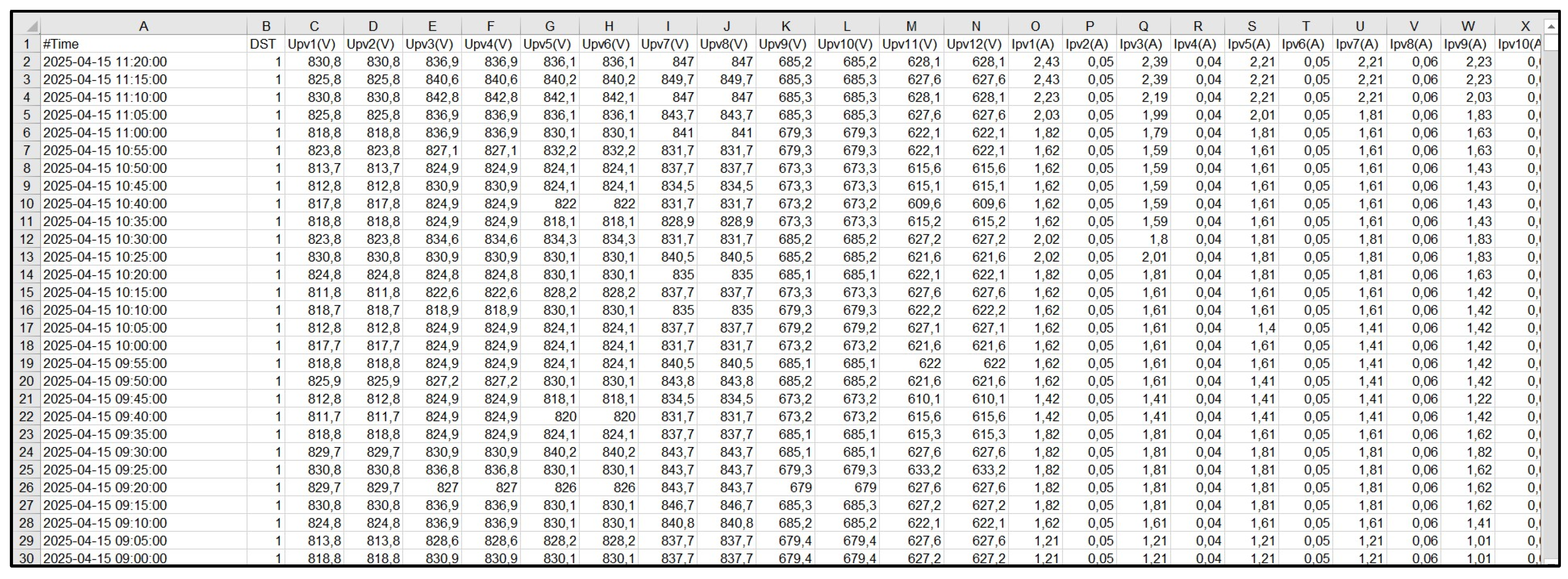
Figure 2.
Diurnal profile: Median & IQR.
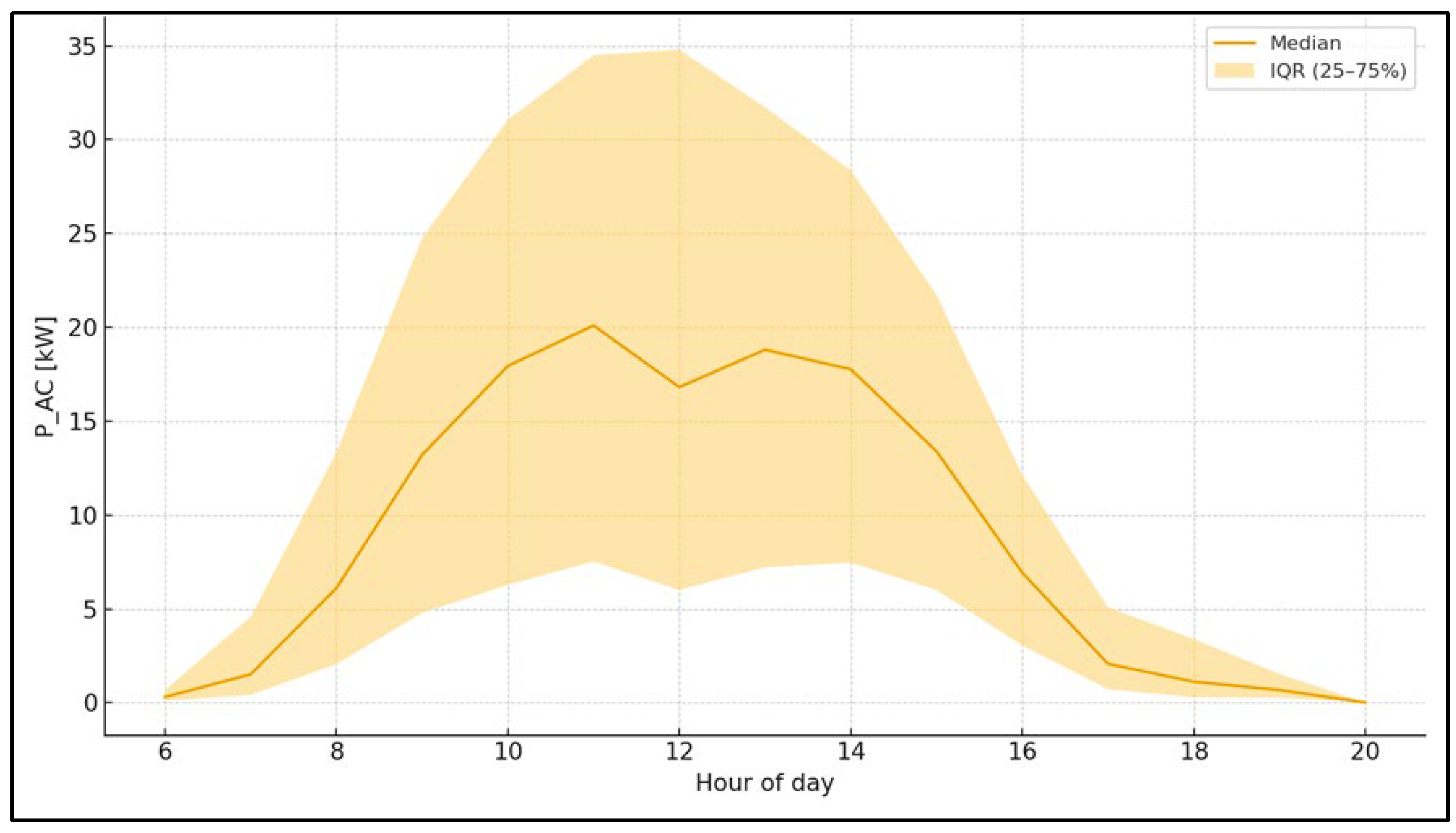
Figure 3.
Histogram of (daylight).
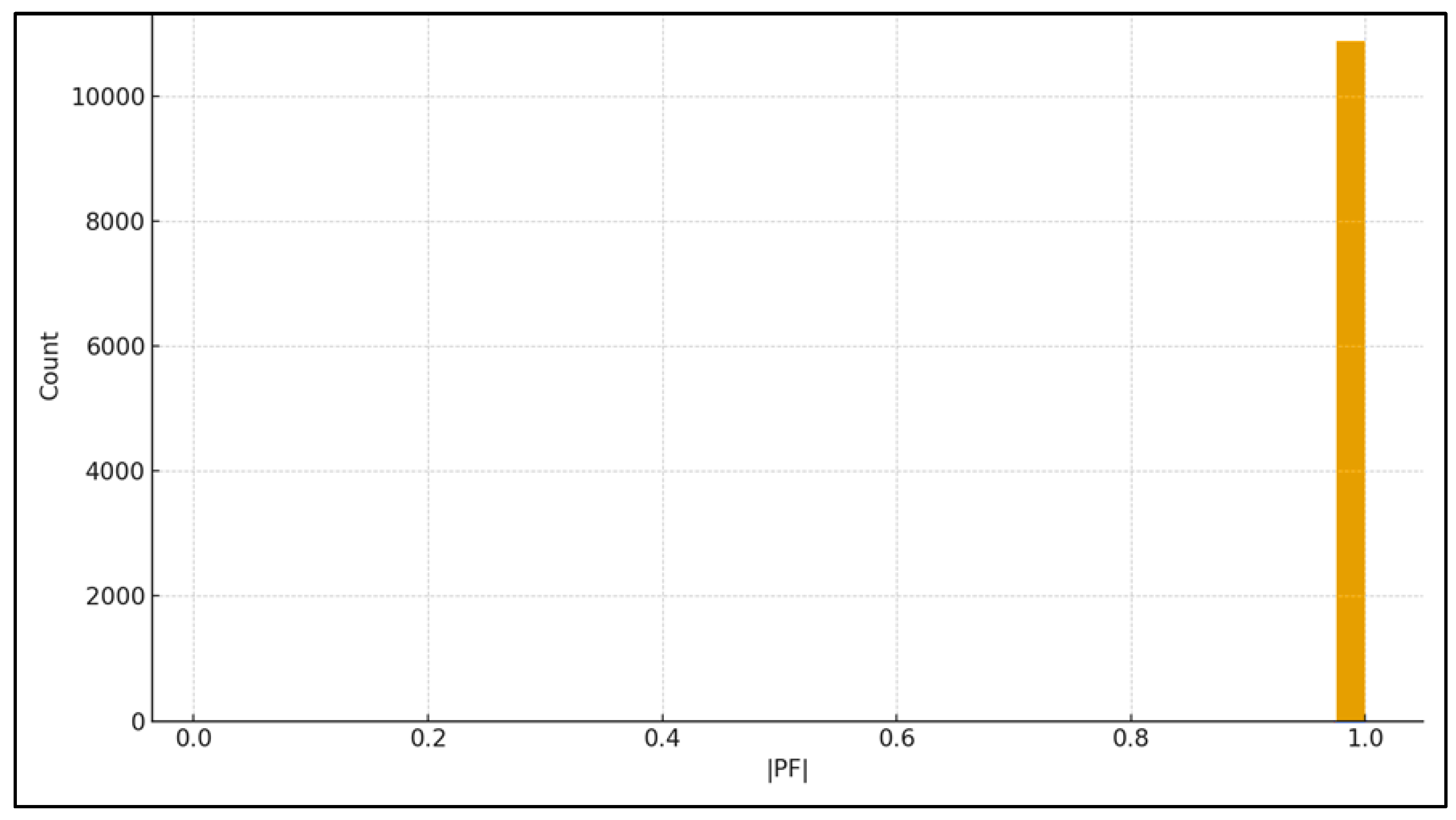
Figure 4.
Ramp-rate distribution.
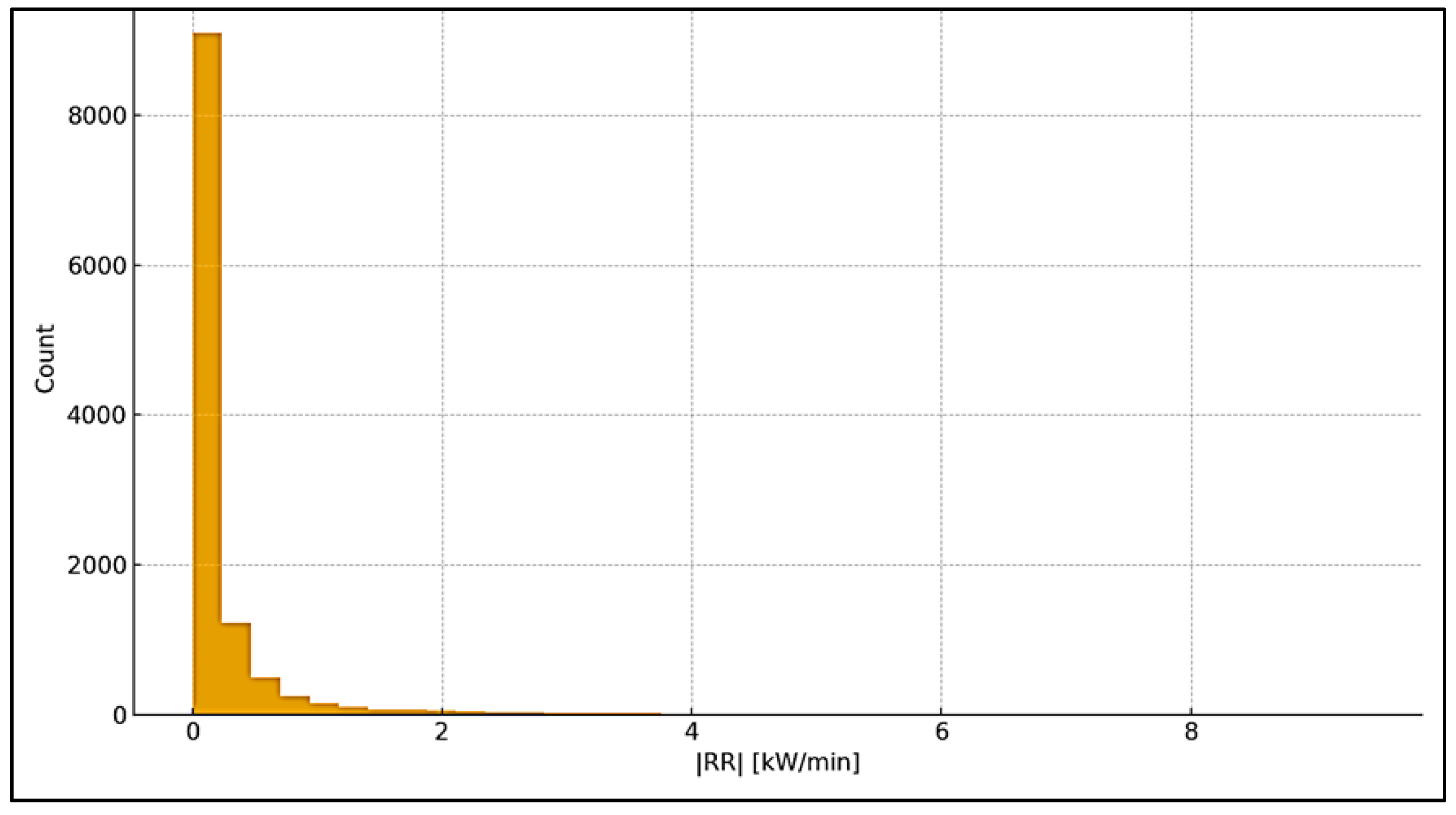
Figure 5.
scatter (daylight).
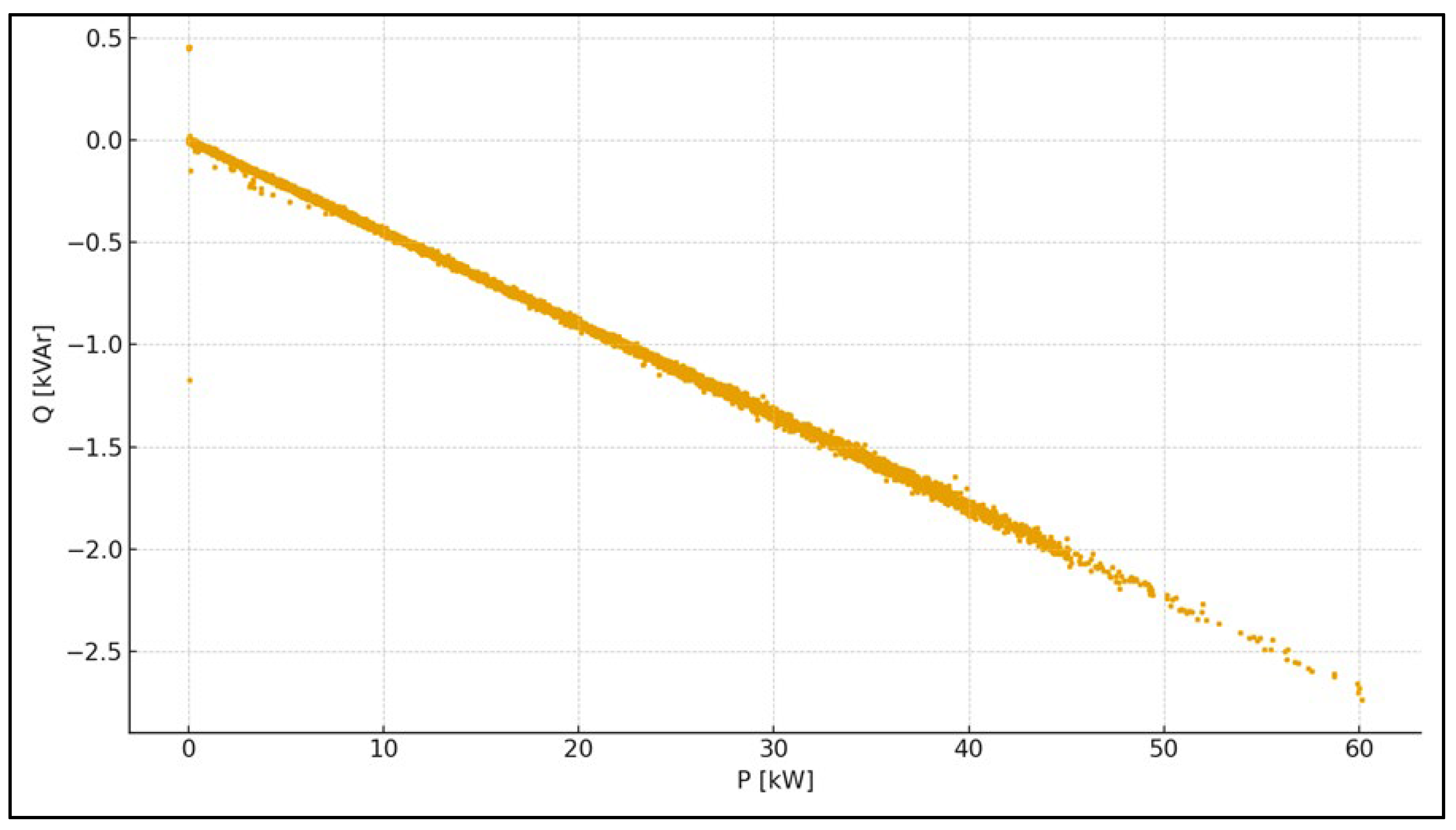
Figure 6.
Inverter efficiency vs .
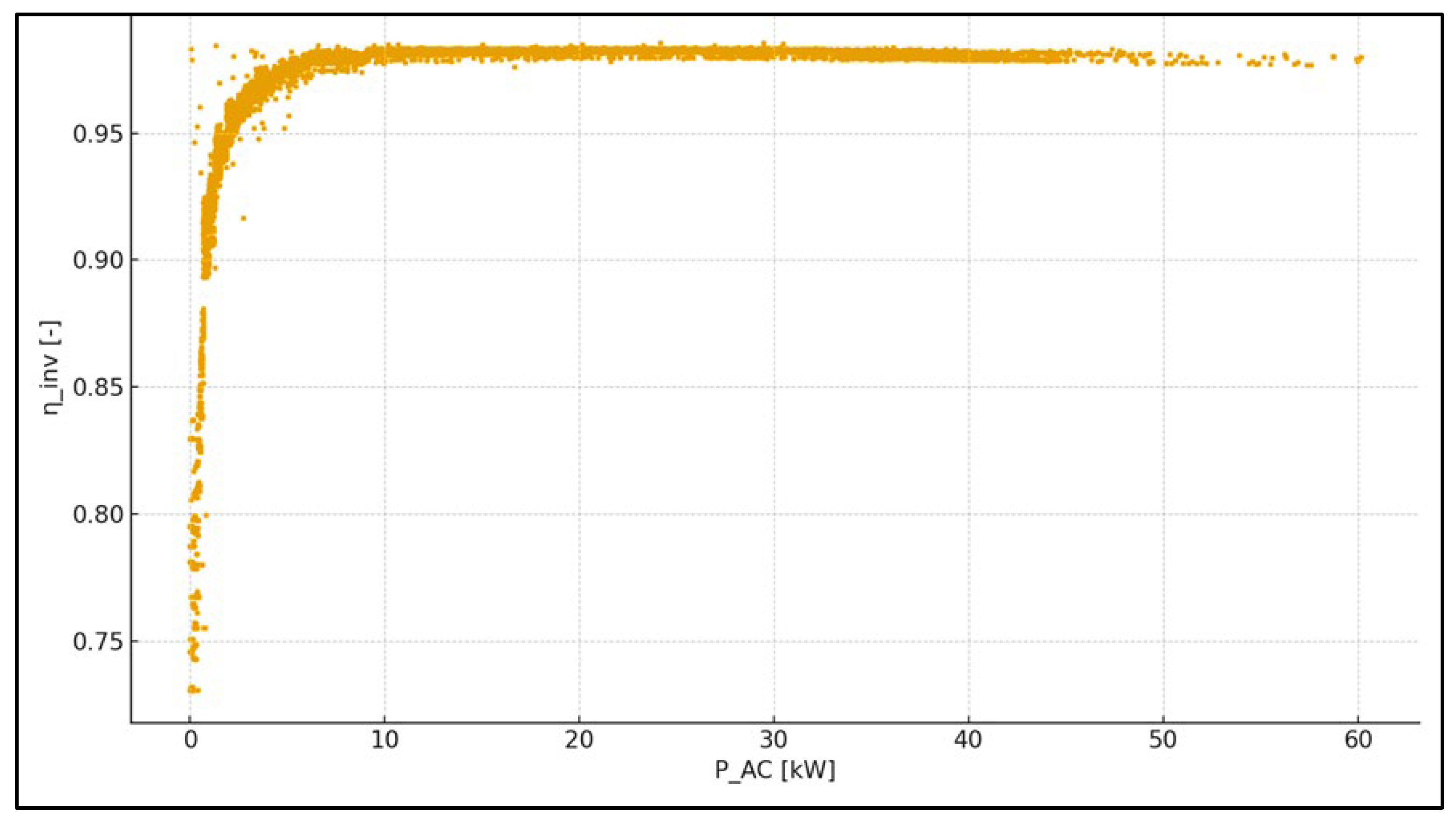
Figure 7.
Best vs worst day.
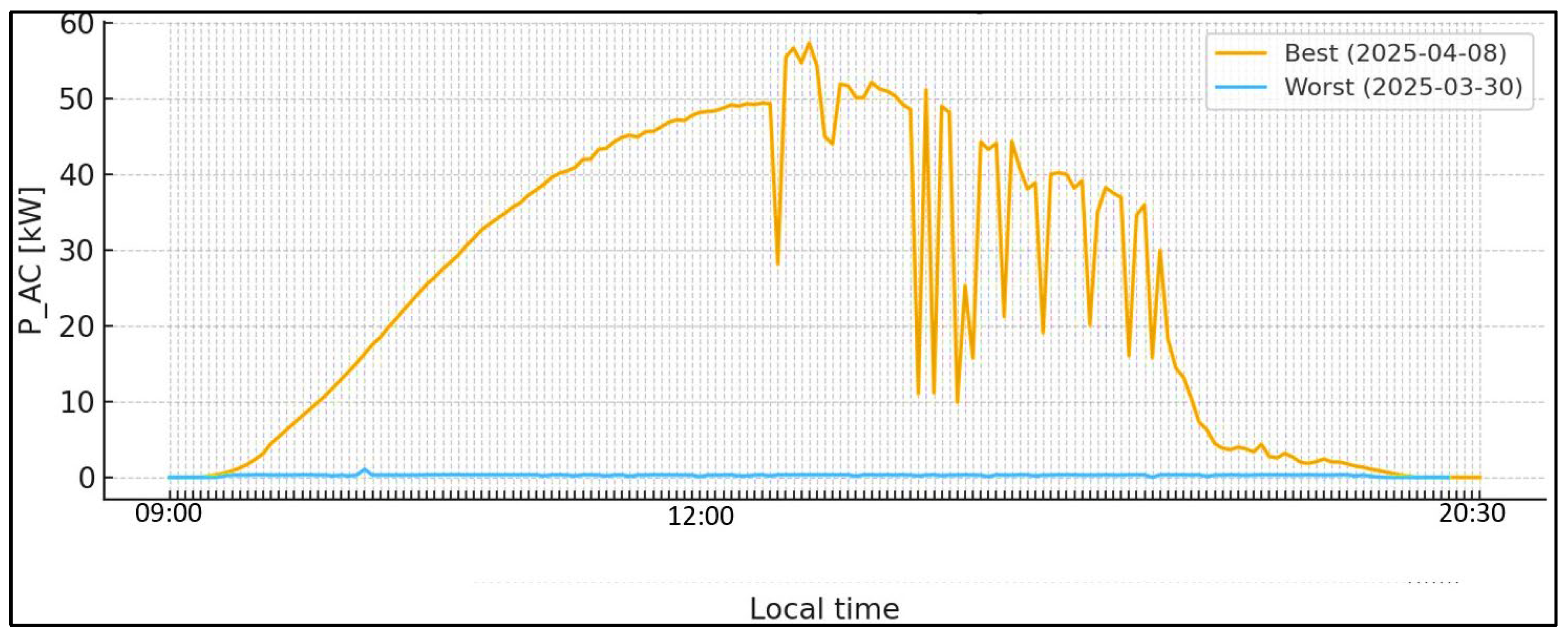
Figure 8.
Cumulative AC energy.
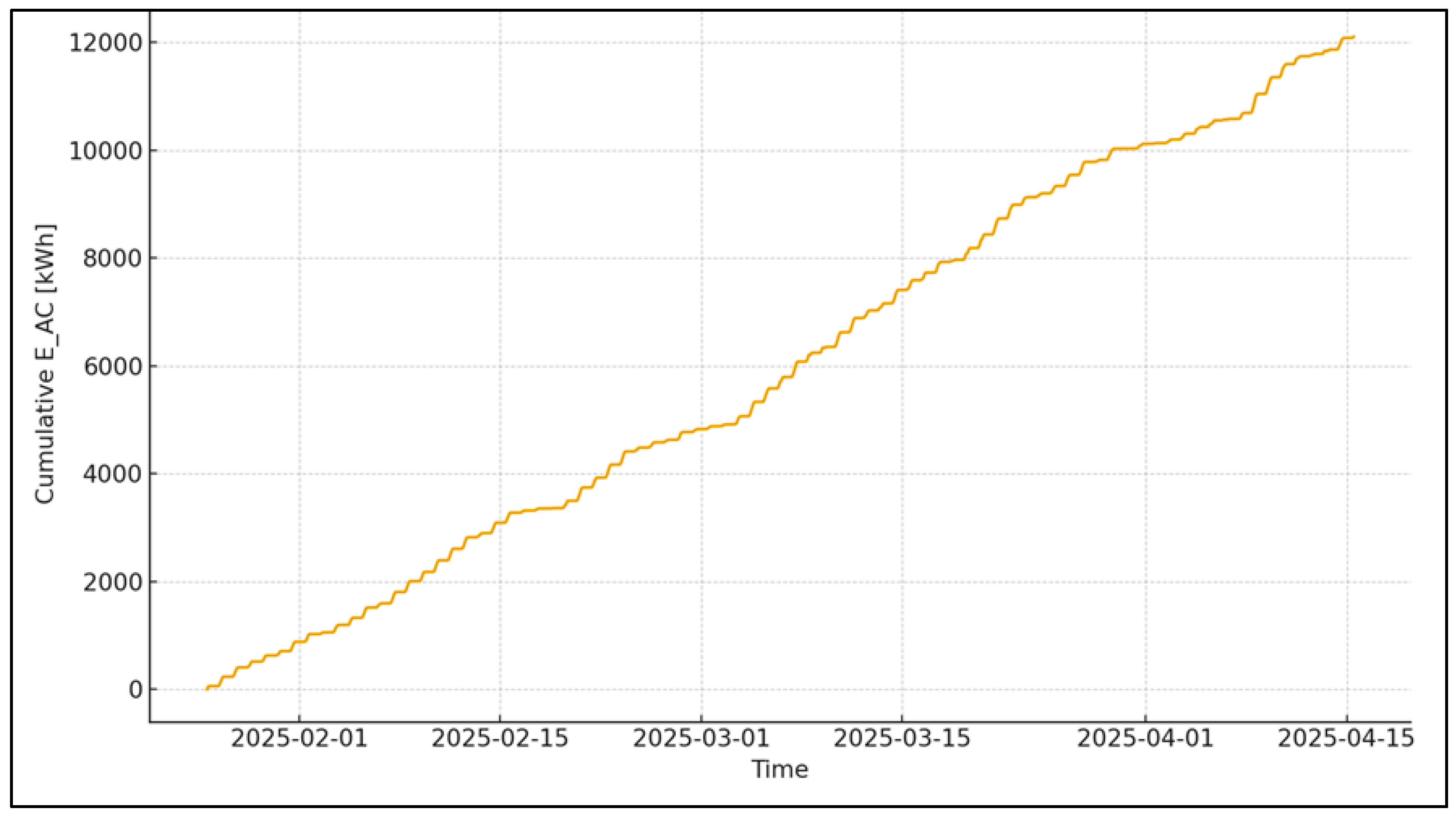
Figure 9.
Daily deficit vs hour-median baseline.
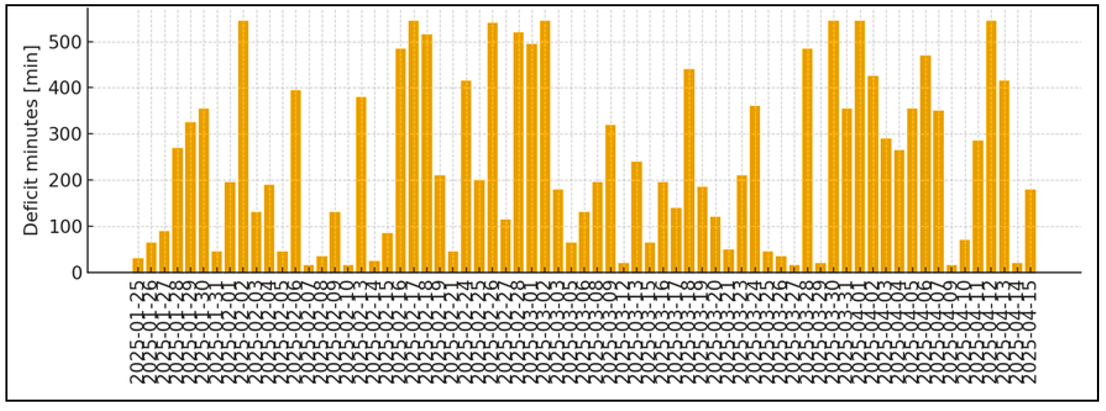
Figure 10.
vs hour-median baseline (sample window).
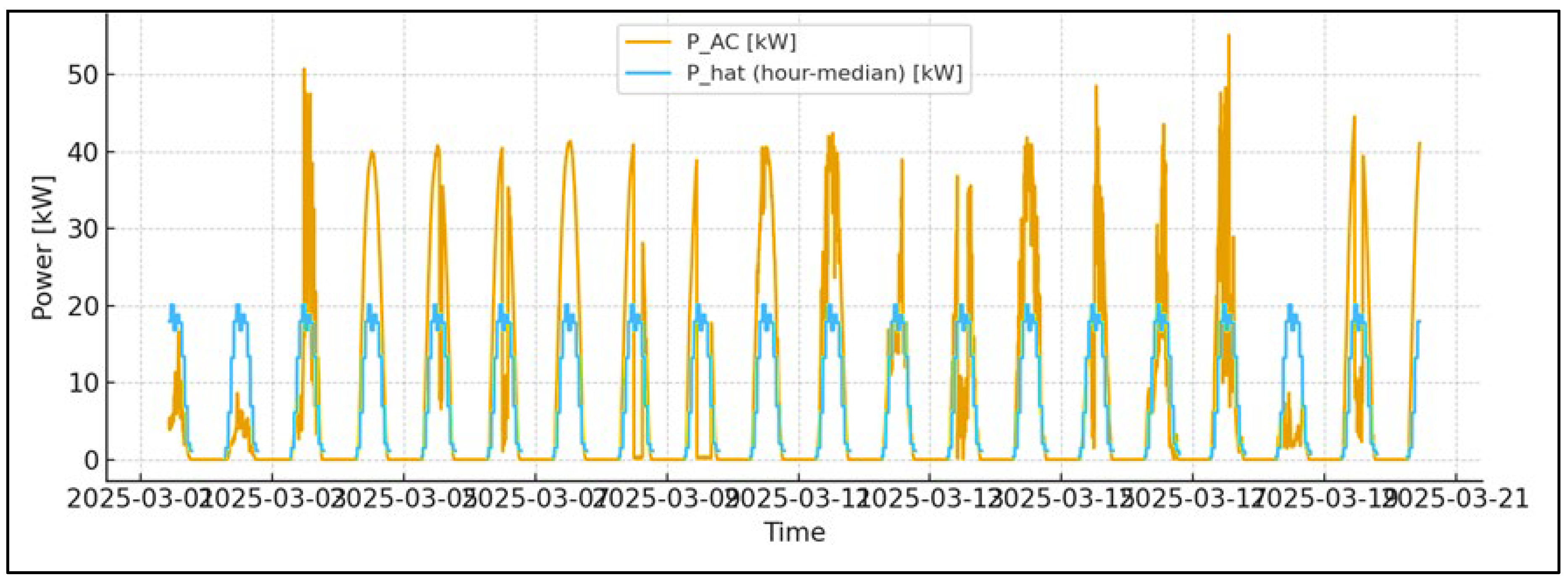
Figure 11.
Daily vs hour-median baseline.
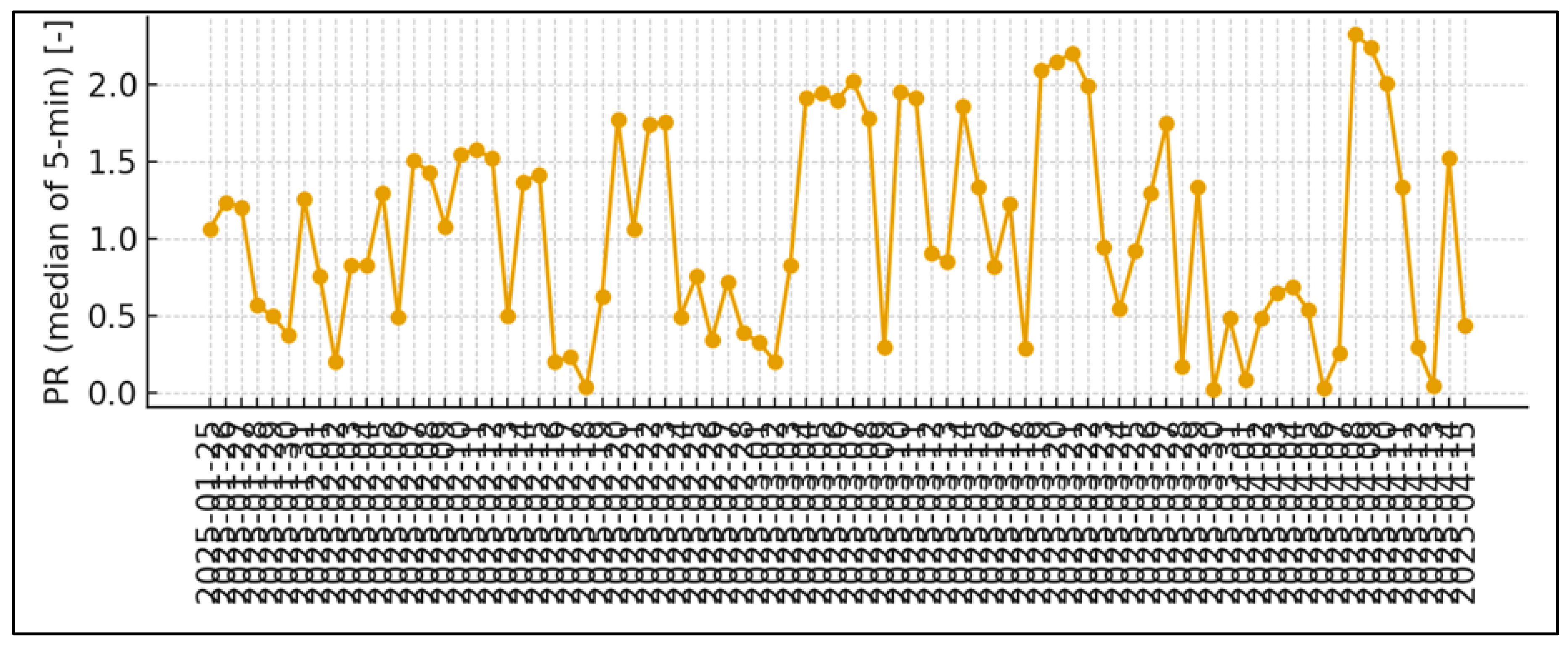
Figure 12.
Cumulative energy – vs hour-median baseline.
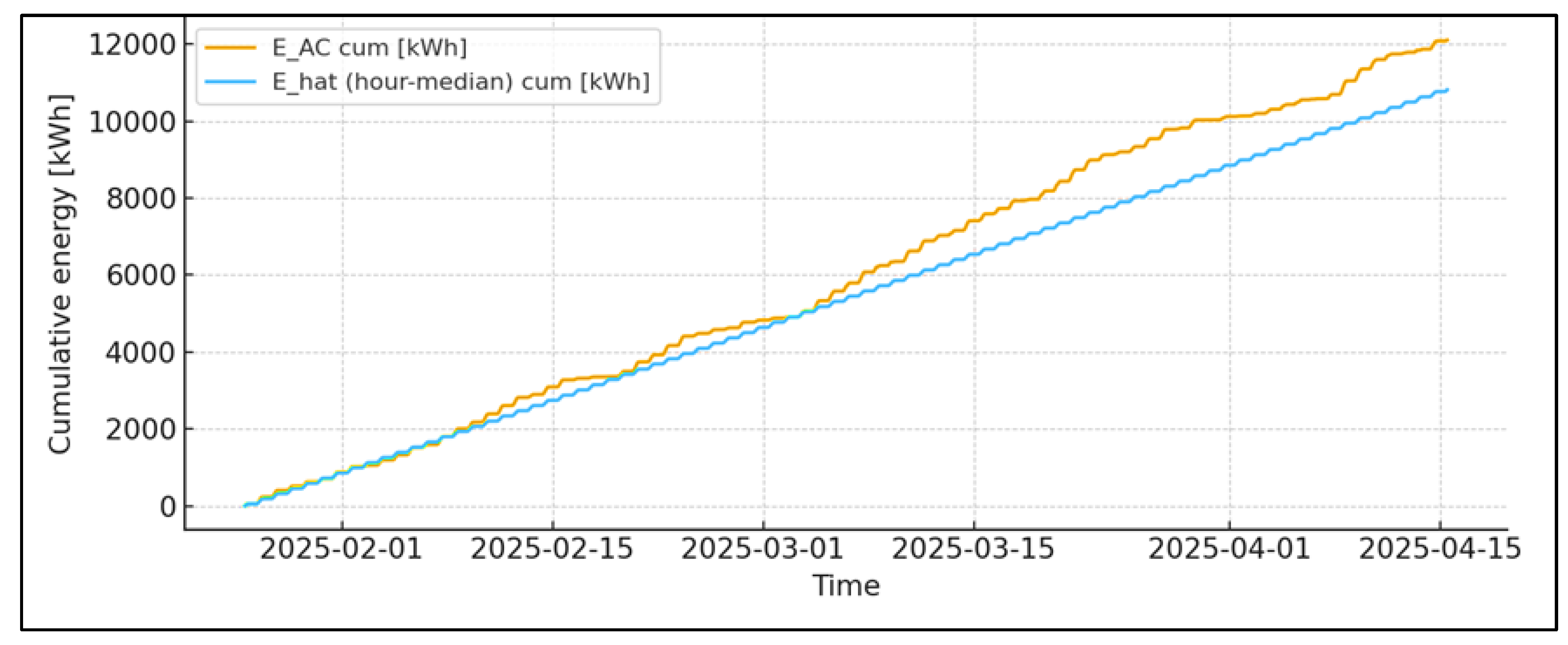

Table 1.
Time, indices, and operators.
| Symbol | Designation | Units | Range / Note |
|---|---|---|---|
| Time Moment (Time index) |
— | Discretization 5 min (Median ) |
|
| Time Step | |||
| Hour of Day | |||
| Calendar Date | — | Local Time (Europe) | |
| Sum of Times | — | For Energies/Units | |
| Median | — | Sustainable Statistics | |
| -percentile (quantile) | — | e.g., , | |
| IQR | Inter-Quartile Range | — | |
| Positive Part | — | ||
| ( | \cdot | ) | Absolute Value |
Table 2.
SCADA measurements (main channels).
| Symbol | Designation | Units | Range / Note |
|---|---|---|---|
| DC Power to Inverter | From | ||
| Inverter Efficiency | — | From | |
| AC Active Power | Restored: | ||
| Reactive Power | From | ||
| Power Factor (Sign) | — | From | |
| ( | \mathrm{PF} | (t)) | Absolute |
| Aggregated DC Voltage | Average of | ||
| Aggregated DC Currents | A | Average of |
Table 3.
Derived quantities and energies.
| Symbol | Designation | Units | Range / Note |
|---|---|---|---|
| Total Produced Energy | |||
| Daily Energy | |||
| Ramp-Rate | over 5 min | ||
| ( | _{95}) | 95th percentile of ( | |
| , | Percentile Levels | For "upper" levels | |
| Observed Maximum | No clipping if no plateau |
Table 4.
Internal (operational) bases and indicators.
| Symbol | Designation | Units | Range / Note |
|---|---|---|---|
| Internal Hourly Median Power | "Typical Day" (Weather-Sensitive) |
||
| Cumulative Energy on an Internal Basis | |||
| Operational Relative to | — | Median of per day | |
| "Deficit" Intervals | — | Segments | |
| Total Deficit Relative to |
Table 5.
Climate references and models.
| Symbol | Designation | Units | Range / Note |
|---|---|---|---|
| Climate Reference Power (Total) |
PVGIS/PECD/NASA model | ||
| Expected PV Power from PVGIS | By geometry/losses | ||
| PVGIS Power Normalized (per 1 ) |
For scale calibration | ||
| Scale to Real Capacity | |||
| Capacity Factor (PECD) |
— | 0…1 | |
| Scale to | |||
| Regressive (NASA) |
|||
| Global Radiation at Horizon | NASA POWER: hourly | ||
| Temperature at 2 m | NASA POWER | ||
| Wind at 10 m | m/s | NASA POWER |
Table 6.
KPI against climate base.
| Symbol | Designation | Units | Range / Note |
|---|---|---|---|
| Daily | — | ||
| Overall | — | ||
| Climate-Friendly "Deficit" (Curtailment) |
|||
| Residual against |
Table 7.
Geometry/design parameters.
| Symbol | Designation | Units | Range / Note |
|---|---|---|---|
| Zenith Angle of the Sun | ° | in Geometric Base | |
| Exponent in Geometric Base | — | ||
| Inclination of the Modules | ° | PVGIS parameter | |
| Azimuth (0°= South) | ° | PVGIS parameter | |
| ILR | DC:AC coefficient (Inverter Loading Ratio) |
— | Design parameter |
Table 8.
Energy quality and limits.
| Symbol | Designation | Units | Range / Note |
|---|---|---|---|
| Point in Plane | |||
| ( | \mathrm{PF} | <0.95) | Deviation Indicator |
| TRIP/RESTART | Shutdown/Restart Events | — | Number and Times of Events |
Table 9.
Energy quality and limits.
| Symbol | Designation | Units | Range / Note |
|---|---|---|---|
| Weight in Regression/Calibration | — | Larger on clear afternoons | |
| Set of "Pure" Intervals | — | For calibration | |
| Indicator Function | — | Optionally in Algorithms |
Disclaimer/Publisher’s Note: The statements, opinions and data contained in all publications are solely those of the individual author(s) and contributor(s) and not of MDPI and/or the editor(s). MDPI and/or the editor(s) disclaim responsibility for any injury to people or property resulting from any ideas, methods, instructions or products referred to in the content. |
© 2025 by the authors. Licensee MDPI, Basel, Switzerland. This article is an open access article distributed under the terms and conditions of the Creative Commons Attribution (CC BY) license (http://creativecommons.org/licenses/by/4.0/).
Copyright: This open access article is published under a Creative Commons CC BY 4.0 license, which permit the free download, distribution, and reuse, provided that the author and preprint are cited in any reuse.


