Submitted:
20 November 2024
Posted:
22 November 2024
You are already at the latest version
Abstract
With the global energy mix transformation, new energy resources, particularly luminous energy, have garnered increasing attention, along with a gradual increase in their proportion in the electric power sector. However, challenges in new energy resource consumption and system planning persist. This study develops a power supply planning model that improves the consumptive ability of new energy resources. Specifically, this study presents a power supply planning model based on a photovoltaic (PV) microgrid system. System modeling and simulation analysis were conducted using MATLAB/Simulink, analyzing the output characteristics of PV microgrid system optimization. Initially, models for PV power and direct current load were established, and the effects of different parameters on the power curve were analyzed. The results demonstrate that the mathematical models are effective in simulating the output characteristics of PV microgrid systems. Additionally, the model optimized the power supply, supporting the sustainable development of the power system. Adjusting the model’s parameters significantly influences the system output, which is valuable for designing and optimizing PV power generation systems.
Keywords:
photovoltaic DC microgrid
; power output
; simulation model
; output characteristics
1. Introduction
With the rapid depletion of fossil fuels, there has been growing interest in the development of renewable energy sources. New energy resources, such as solar, wind, hydro, geothermal, and bioenergy are garnering significant attention [1,2]. Among these luminous energy is a critical component owing to its minimal environmental impact. The energy conversion process produces almost no pollutants and requires no additional resources compared with traditional fossil fuels, making it environmental friendly [3,4]. With advancement in photovoltaic (PV) technology, the construction and operation of PV power generation systems have become significant drivers of economic growth. In the late 20th century, scientific researchers discovered the phenomenon of the PV effect, where sunlight illuminating the surface of semiconductor materials generates an induced current [5,6]. Technological advancement have led to the successful development of monocrystalline Si solar cells, making a breakthrough in solar-to-energy conversion [7].
In traditional energy systems, distribution networks primarily use alternating current (AC) [8]. Recently, researchers have proposed a direct current (DC) microgrid to reduce energy conversion loss in transmission systems. This approach reduces the power conversion and DC load conversion losses, enhancing economic efficiency. It also avoids synchronization with large AC power grids [9,10]. For security, the bus voltage remains stable during power outages or voltage drops owing to the high energy storage capacity of the DC capacitor and converter voltage control [11,12]. This study presents a power-plan mathematical model based on a PV microgrid.
2. Simulation Construction of Photovoltaic Microgrid
The primary modules of PV microgrid include a PV cell, boost converter, and DC load. This system forms a compact microgrid model, as illustrated in Figure 1.
2.1. Photovoltaic Cell Modeling
The current in the system is determined by the output power of the PV array. The output current of the solar cell is calculated using Equation (1):
where I denotes the output current; Iph is the photocurrent; Is is the reverse saturation current; q is the elementary charge; V is the voltage; n represents the reverse saturation current coefficient; k is Boltzmann’s constant; and T denotes temperature. This equation is commonly used to calculate the PV cell output current. However, the accurate value of , , are difficult to obtain [13]. To accurately calculate the output current, relevant parameters can be adjusted to simplify Equation (1), as shown in Equation (2):
For simplicity, Equation (2) can be replaced by Equation (3), where B represents the battery capacity:
To simplify the calculation at room temperature, the value of exceeds one, as shown in Equation (4):
To precisely represent the state of the electric circuit, we obtain Equation (5):
When significantly exceeds one, the battery capacity is given by Equation (6):
Equations 2 to 6 can be incorporated into a simulation model, from which the voltage–current(U-I) characteristic curve of the PV power can be obtained.
After obtaining the U-I characteristics, the values of light intensity and system temperature variation are calculated [14]. Subsequently, these values are substituted into Eq. 7 and used in the simulation:
The simulation model of the PV power is developed using the MATLAB/Simulink simulation software, as shown in Figure 2.
The packaged simulation model of PV power is illustrated in Figure 3.
2.2. DC Load Modeling
Compared with PV power, establishing a DC load model is more convenient. The RLC load is selected using the Simscape module, as shown in Figure 4.
2.3. DC Microgrid Modeling and Parameters Setting
After modeling each module, a DC microgrid simulation model is built using Simulink, as depicted in Figure 6. The elapsed time is set as 3 s, while the discrete step is set at 5×10⁻⁷ s.
The simulation environment is set as a discrete state, and the ode23tb simulation algorithm is used. Other simulation parameter settings, including the maximum and minimum step sizes, are illustrated in Figure 7.
The important parameters of each simulation components are presented in Table 1.
3. System Simulation Results and Analysis
3.1. Output Characteristic Analysis of Photovoltaic Cell
The power–voltage (P-V) characteristics of the PV array are shown in Figure 8. When the operating voltage of the generator is lower than the maximum voltage Vmax, the output voltage of the array increases [16,17,18]. However, when the operating voltage exceeds Vmax, the output voltage gradually decreases, leading to a reduced output power of the array [19,20]. From the curve graph, the PV array performance can be optimized automatically using maximum power point tracking (MPPT) technology [21]. According to the voltage regulation on the console, the output power of the PV array can be adjusted under varying temperatures and lighting conditions, which improves efficiency.
Studies have demonstrated that fluctuations in temperature and light intensity continuously affect the output power, no-load voltage, and short-circuit current of PV arrays. These environmental changes alters the system’s equilibrium points reducing efficiency and impacting the rate of energy conversion [22,23,24]. Therefore, the adaptability of the system to environmental changes must be improved. Power variation under different situations must be constantly monitored to maintain maximum power output (MPO). Therefore, a detailed system-control strategy must be explored. Consequently, the output characteristics of PV cell are analyzed.
(1) I/U and P/U characteristic curves under constant temperature and light intensity
The operating temperature of PV unit is set at constant 25 ℃, with simulations of the effects of different light intensities on PV array shown in Figure 9.
From Figure 9a, under a constant ambient temperature (25 ℃), battery current increases with increasing light intensity. Additionally, the open-circuit voltage (VOC) slightly increases, but its growth rate is lower than that of the electric current. This indicates that electric voltage is less sensitive to changes in illumination [25,26]. A single parabolic peak is observed in the P-U characteristic diagram. At 25 ℃, the battery output power positively correlates with light intensity, but beyond the maximum power point, system power decreases despite an increase in voltage. In Figure 9b, the maximum power point is also positively correlated with light intensity. Therefore, under constant ambient temperature, the output power of the PV module positively correlates with light intensity.
(2)I/U and P/U characteristic curves for the same light intensity and temperature
After the light intensity of the PV unit is set to 1000 W/m2, the effects of different temperatures on the PV array are simulated, as shown in Figure 10.
As shown in Figure 10a, with increasing temperature, the electric voltage decreases as electric current also increases. This change is more significant at different temperatures. Figure 10b shows that the temperature increases with decreasing output power, which explains the inverse proportionality between maximum power and temperature. Consequently, under constant light conditions, an increase in temperature causes the output photovoltaic (OPV) device voltage to decrease while increasing the current, ultimately reducing output power. By contrast, when the temperature decreases, the property parameters of the PV device exhibit a reverse trend.
According to these two simulation experimental results, the effects of ambient temperature and light intensity on the output characteristics of the PV device can be explored. Among these factors, light intensity has a more significant effect on the device’s properties. Additionally, the output current of PV device is directly proportional to the light intensity, while the output voltage of the PV device is inversely proportional to the temperature. Therefore, the sensitivity of the PV device to the light intensity is higher than that to the temperature.
3.2. Calculation Process of Maximum Power Algorithm
The maximum power algorithm significantly affects output characteristics. Variations in temperature and light intensity can affect the maximum power point of a PV cell, as well as its output voltage and current. To improve the PV cell properties for practical applications and increase the energy-conversion efficiency, a boost inverter is used to adjust the PV cell. This adjustment, which involves changes in the battery power, is an effective control method, as illustrated in Figure 11. Owing to the maximum power control structure, a PV cell can approach or reach the MPO in different environments.
The Incremental Conductance Method(INC) was used for MPPT control. Instantaneous conductivity changes in PV array can be monitored, and the MPPT can be defined. Photovoltaic cell conductivity changes with MPPT. The MPPT corresponds to the point at which the conductivity changes significantly. In this study, the MPPT realization by incremental conductance followed these steps.
(1) The voltage(U) and power(P) of PV cell were measured.
(2) The rate of change in the conductivity(G) was calculated as dG/dV.
(3) The maximum power point is confirmed when dG/dV=0.
With this method, additional sensors and complicated mathematical models are not required. MPPT can be found only with voltage and current measurements. Additionally, the incremental conductance algorithm is robust to the nonideal characteristics of PV cells and environmental changes.
As illustrated in Figure 12, the operating points are continuously adjusted using the incremental conductance algorithm. The PV cell always operates around the MPPT. This method can significantly improve the energy utilization of PV systems, from which solar energy can be maximally used. Based on accurate control and optimization, MPPT technology plays an important role in the field of PV power generation.
The control process of incremental conductance algorithm is shown in Figure 13.
In Figure 13, the duty cycle variation isΔD. MPPT is defined as the change in dG/dV. In MPPT, the value of dG/dV changed from positive to negative. The duty cycle was adjusted to search for MPPT. This is a function of tracking control. In Figure 13, V(k) and I(k) represent the latest detected voltages and currents, respectively. V(k-1)、I(k-1) are previous detected voltage and current. the D-values of the latest and previously detected values were calculated. K is a variable coefficient with a value is 5-10.
4. Simulation of Different Influence Factors on Output Power Situation
Based on the output characteristics of PV cell, the maximum output power of PV array was affected by the MPPT algorithm, light intensity, and temperature. Therefore, a wide-range and fast-response incremental conductance algorithm was used as the MPPT control algorithm. The simulation module is illustrated in Figure 14.
In Figure 14, U and I are the first inputs. Subsequently, the rate of signal change is calculated. MPPT is obtained using dV=0. The step length is set at -0.01.
The control structure of duty cycle is shown in Figure 15.
4.1. Effect of Different Light Intensity on Output Power Situation
The constant temperature and initial light intensity are set at 25 ℃ and 1000 W/m2, respectively. The light intensity at 1 s fluctuates at 500 W/m2 and increases to 800 W/m2 after 2 s. The PV panel parameters and light intensity change curves are listed in Table 2.
The light intensity variation curve is shown in Figure 16.
The effects of different lighting conditions on PV array output results are shown in Figure 17, which shows the actual output voltage and current of PV array.
As shown in Figure 17a, the PV output voltage fluctuates at approximately 34.5V within 0.12 s,. Although the light intensity changed, the voltage fluctuation remains small. As shown in Figure 17b, during the initial stage of the simulation, the output current rapidly reaches 7.5A, which aligns with the initial PV panel setup parameters. The current waveform can be clearly observed according to the partial enlargement of the oscilloscope. However, with changes in light intensity, the fluctuation becomes more pronounced. According to the PV output curve shown in Figure 17c, the incremental conductance is flexibly adjusted. Within 0.12 s, the MPPT is rapidly tracked, which outputs power. With changes in light intensity, the control algorithm continues to adjust, identifying the maximum output point.
4.2. Effect of Different Temperatures on Power Output
The light intensity is set to 1000 W/m2, and the initial temperature to 25 ℃. The temperature rises to 35 ℃ in 1 s and decline to 30 ℃ in 1.5 s thereafter. In 2.5 s, the temperature declines again to 25 ℃. The PV panel parameters are listed in table 2, and the temperature curves are shown in Figure 18.
The effects of different temperatures on the power output of the PV array are shown in Figure 19, along with the actual output voltages and currents.
From Figure 19a, in 0.16 s, the PV output voltage fluctuates by approximately 34.5 V. Although the temperature changes, the voltage fluctuation is minimal.
As shown in Figure 19b, in the initial stage of the simulation, the output current quickly reaches 7.5 A, which aligns with the initial PV panel setup parameters. The current waveform can be clearly observed according to the partial enlargement of the oscilloscope. However, with changes in temperature, the current change is insignificant. According to the PV output curve shown in Figure 19c, the incremental conductance is flexibly adjusted. In 0.16 s, the MPPT is quickly tracked, which outputs power. The maximum power output did not change with changes in temperature.
Overall, the primary factors affecting the maximum power output are light intensity changes and the MPPT algorithm, with the effect of light intensity being the most significant. According to the controlled experiment, the power prediction trend conformed to the output characteristics of the PV cell.
5. Conclusions
With rapid socioeconomic development, traditional energy-supplying modes cannot meet the demand for overall growth. PV energy, a renewable and clean energy source, holds wide application prospects. According to the deployment analysis of the PV power generation theory, the following conclusions can be drawn:
(1) The working characteristics and principles of the PV supply were analyzed, exploring the characteristics and advantages of the PV supply. According to an analysis of PV microgrid construction object, the incremental conductance was used for power planning.
(2) PV cells in the microgrid were modeled using the PV cell module in Simulink, and the DC load module was modeled using the RLC load in an electrical storehouse. Subsequently, the simulation parameters were defined.
(3) The output characteristics of the PV power supply and output were simulated. Test results showed that with increasing temperature, system output power and voltage declined, and vice vera. Thus, temperature changes are inversely proportional to the output characteristics of PV power generation, although, the effect was minimal.
(4) The effect of light intensity on the PV power generation output characteristics was significant. When light intensity significantly changed (from 1000 w/m2 to 600 w/m2), the output power of the PV system became unstable. This observation suggested that the performance of the PV system was poor under weak light intensities. Thus, a DC boost circuit can improve output stability.
Author Contributions
Conceptualization, Y.C. and G.Y.; methodology, G.Y.; software, Y.C.; validation, G.Y.; formal analysis, G.Y.; investigation, Y.C.; resources, Y.C.; data curation, G.Y.; writing—original draft preparation, G.Y.; writing—review and editing, G.Y.; visualization, Y.C.; supervision, Y.C.; project administration, Y.C.; funding acquisition, Y.C. All authors have read and agreed to the published version of the manuscript.
Funding
This research was aided by the key area campaign of regular universities in Guangdong province, No. 2021ZDZX1058. The Feature Innovation project of regular universities in Guangdong province, No. 2022KTSCX194. The offshore wind power joint funding project in Guangdong province, No. 2023A1515240063. The key area campaign of regular universities in Guangdong province, No. 2024ZDZX4074.
Institutional Review Board Statement
Not applicable.
Informed Consent Statement
Not applicable.
Data Availability Statement
Data is contained within the article.
Conflicts of Interest
There are no conflicts of interest.
References
- Souilem, M.; Zgolli, N.; Cunha, T.R.; Dghais, W.; Belgacem, H. Signal and Power Integrity IO Buffer Modeling Under Separate Power and Ground Supply Voltage Variation of the Input and Output Stages. IEEE Transactions on very Large Scale Integration (VLSI) Systems 2023, 31, 874–886. [Google Scholar] [CrossRef]
- Liu, W.; Zhang, H. Ripple-Responce Modeling and Design-Oriented Analysis of Output Common Power Flow Regulation in Bipolar SIDO DCDC Converters. IEEE Transactions on Industrial Electronics 2024, 71, 473–483. [Google Scholar] [CrossRef]
- Zhang, Y.L.; Zhang, J.G.; Chen, Y.J. An optimal capacity allocation method for integrated energy systems considering uncertainty. AIP Advances 2023, 13, 085325. [Google Scholar] [CrossRef]
- Yang, J.J.; Guenter, S.; Buticchi, G.; Gu, C.Y.; Liserre, M.; Wheeler, P. On the Impedance and Stability Analysis of Dual-Active-Bridge-Based Input-Series Output-Parallel Converters in DC Systems. IEEE Transactions on Power Electronics 2023, 38, 10344–10358. [Google Scholar] [CrossRef]
- Li, Z.W.; Li, H.Y.; Sun, S.H. Virtual Model Predictive Control for Inverters to Achieve Flexible Output Impedance. Shaping in Harmonic Interactions with Weak Grids. IEEE Transactions on Power Electronics 2024, 39, 10754–10767. [Google Scholar] [CrossRef]
- Wei, J.; Yang, W.J.; Li, X.D.; Wang, J.S. Data-Driven Modeling for Photovoltaic Power Output of Small-Scale Distributed Plants at the 1-s Time Scale. IEEE Access 2024, 12, 117560–117571. [Google Scholar] [CrossRef]
- Xu, F.; Guo, Y.J.; Zhang, X. An Enhanced Quasi-CC Output Model of LCC-P Compensated Inductive-Power-Transfer Converters. IEEE Transactions on Power Electronics 2023, 38, 15126–15130. [Google Scholar] [CrossRef]
- Yang, H.J.; Niu, W.Q.; Wang, X.T.; Gu, W. ; Wind turbine output power forecasting based on temporal convolutional neural and complete ensemble empirical mode decomposition with adaptive noise. International Journal of Green Energy 2023, 20, 1612–1627. [Google Scholar] [CrossRef]
- Meng, X.Y.; Liu, Z.G.; Liu, Y.M.; Zhou, H.; Tasiu, I.A.; Lu, B.; Gou, J.; Liu, J.W. Conversion and SISO Equivalence of Impedance Model of Single-Phase Converter in Electric Multiple Units. IEEE Trnsactions on Transportation Electrification 2023, 9, 1363–1378. [Google Scholar] [CrossRef]
- Wang, X.S.; Jiang, C.Q.; Zhou, J.Y.; Mo, L.P.; Wang, Y.B. Enhanced Modeling of Wireless Power Transfer System with Battery Load. IEEE Transactions on Power Electronics 2024, 39, 6574–6579. [Google Scholar] [CrossRef]
- Ma, D.C.; Xie, R.Y.; Pan, G.B.; Zuo, Z.X.; Chu, L.D.; Ouyang, J. Photovoltaic Power Output Prediction Based on Tabnet for Regional Distributed Photovoltaic Stations Group. Energies 2023, 16, 5649. [Google Scholar] [CrossRef]
- Tang, J.; Liu, J.F.; Wu, J.H.; Jin, G.F.; Kang, H.R.; Zhang, Z.; Huang, N.T. RAC-GAN-Based Scenario Generation for Newly Built Wind Farm. Energies 2023, 16, 2447. [Google Scholar] [CrossRef]
- Alvarez-Arroyo, C.; Vergine, S.; de la Nieta, A.S.; Alvarado-Barrios, L.; D’Amico, G. Optimising microgrid energy management: Leveraging flexible storage systems and full integration of renewable energy sources. Renewable Energy 2024, 229, 120701. [Google Scholar] [CrossRef]
- Wang, S.M.; Yuan, X.H.; Huang, Q.; Chen, A.Q.; Ma, H.B.; Xu, X. Daily consumption monitoring method of photovoltaic microgrid based on genetic wavelet neural network. International Journal of Low-Carbon Technologies 2023, 18, 167–174. [Google Scholar] [CrossRef]
- Wang, W.J.; Li, C.; He, Y.; Bai, H.N.; Jia, K.Q.; Kong, Z. Enhancement of household photovoltaic consumption potential in village microgrid considering electric vehicles scheduling and energy storage system configuration. Energy 2024, 311, 133330. [Google Scholar] [CrossRef]
- Lou, J.W.; Cao, H.; Meng, X.; Wang, Y.X.; Wang, J.F.; Chen, L.Q.; Sun, L.; Wang, M.X. Power load analysis and configuration optimization of solar thermal-PV hybrid microgrid based on building. Energy 2024, 289, 129963. [Google Scholar] [CrossRef]
- Tang, Y.Z.; Xun, Q.; Liserre, M.; Yang, H.Z. Energy management of electric-hydrogen hybrid energy storage systems in photovoltaic microgrids. International Journal of Hydrogen Energy 2024, 80, 1–10. [Google Scholar] [CrossRef]
- Alipour, E.; Dejamkhooy, A.; Hosseinpour, M.; Vahidnia, A. Enhanced frequency control of a hybrid microgrid using RANFIS for partially shaded photovoltaic systems under uncertainties. Scientific Reports 2024, 14, 22846. [Google Scholar] [CrossRef]
- Raza, M.K.; Alghassab, M.; Altamimi, A.; Khan, Z.A.; Kazmi, S.A.A.; Ali, M.; Diala, U. Integration of very small modular reactors and renewable energy resources in the microgrid. Frontiers in Energy Research 2024, 12, 1447781. [Google Scholar] [CrossRef]
- Wang, H.P.; Wu, X.W.; Sun, K.; Du, X.D.; He, Y.L.; Li, K.W. Economic Dispatch Optimization of a Microgrid with Wind-Photovoltaic-Load-Storage in Multiple Scenarios. Energies 2023, 16, 3955. [Google Scholar] [CrossRef]
- Lou, J.W.; Wang, Y.X.; Wang, H.Y.; Wang, J.F.; Chen, L.Q.; Zhang, J.Y.; Istam, M.R.; Chua, K.J. Operation characteristics analysis and optimal dispatch of solar thermal-photovoltaic hybrid microgrid for building. Energy and Buildings 2024, 315, 114340. [Google Scholar] [CrossRef]
- Qalyum, S.; Margala, M.; Kshirsagar, P.R.; Chakrabarti, P.; Irshad, K. Energy Performance Analysis of Photovoltaic Integrated with Microgrid Data Analysis Using Deep Learning Feature Selection and Classification Techniques. Sustainability 2023, 15, 11081. [Google Scholar] [CrossRef]
- Pei, X.G.; Zhao, X.H.; Jia, H.Y.; Wang, H.; Liu, J.P. Fuzzy sliding mode control with adaptive exponential reaching law for inverters in the photovoltaic microgrid. Frontiers in Energy Research 2024, 12, 1416863. [Google Scholar] [CrossRef]
- Szilagyi, E.; Petreus, D.; Paulescu, M.; Patarau, T.; Hategan, S.M.; Sarbu, N.A. Cost-effective energy management of an islanded microgrid. Energu Reports 2023, 10, 4516–4537. [Google Scholar] [CrossRef]
- Stanchev, P.; Vacheva, G.; Hinov, N. Evaluation of Voltage Stability in Microgrid-Tied Photovoltaic systems. Energies 2023, 16, 4895. [Google Scholar] [CrossRef]
- Bo, Y.L.; Xia, Y.H.; Wei, W.; Li, Z.C.; Zhao, B.; Lv, Z.Y. Hyperfine optimal dispatch for integrated energy microgrid considering uncertainty. Applied Energy 2023, 334, 120637. [Google Scholar] [CrossRef]
Figure 1.
Photovoltaic microgrid structure diagram.
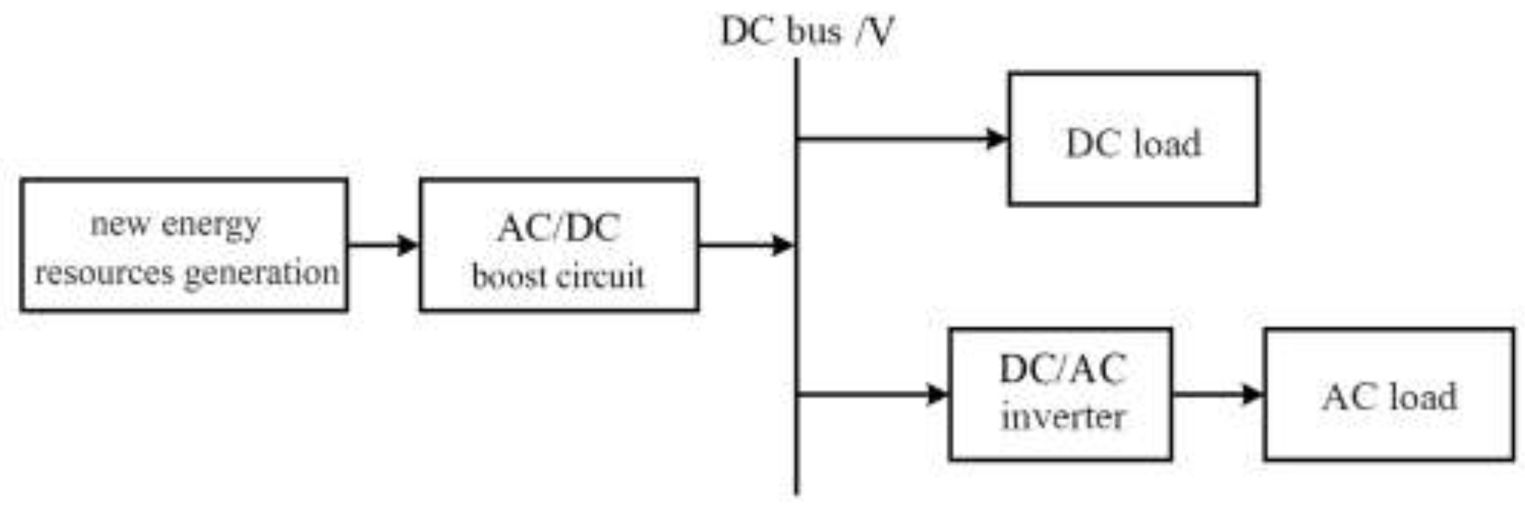
Figure 2.
Photovoltaic cell simulation model.
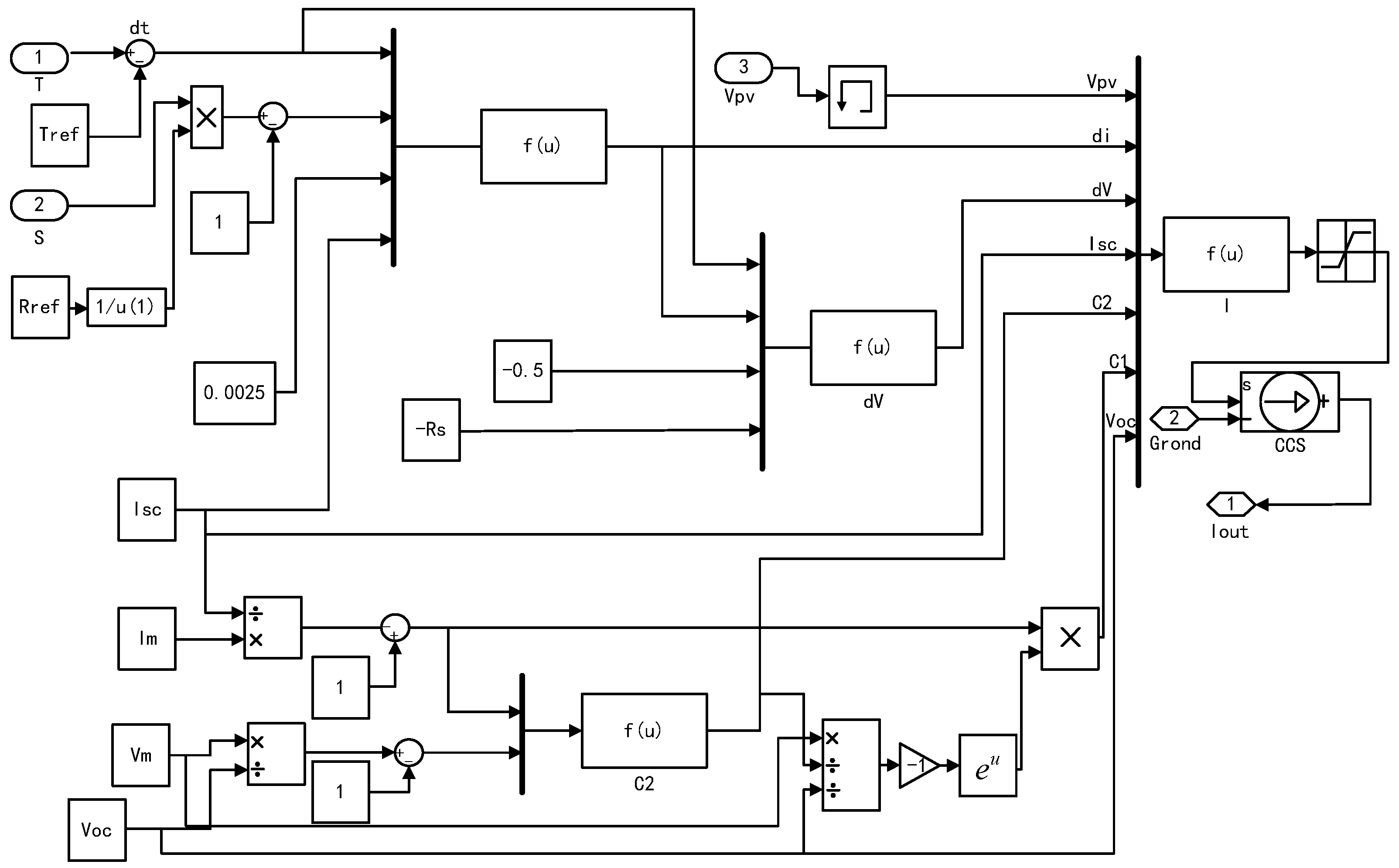
Figure 3.
Photovoltaic cell packaging diagram.
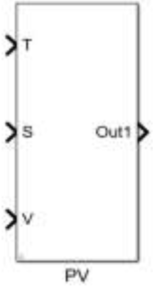
Figure 4.
DC load element.
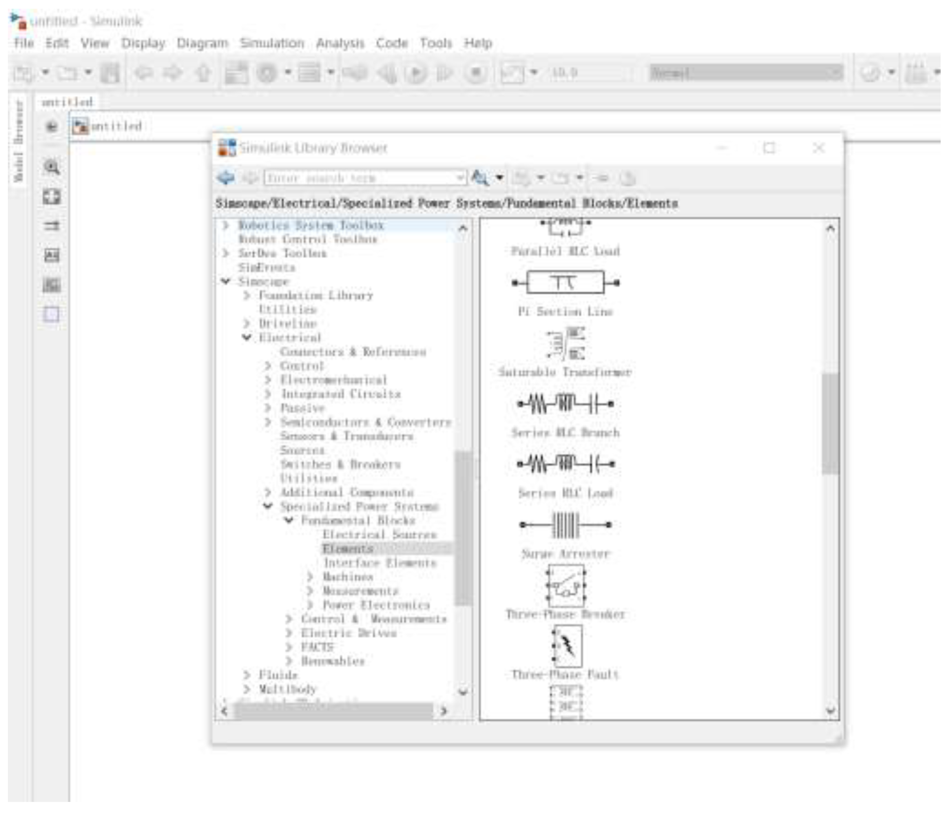
Figure 5.
DC load system.
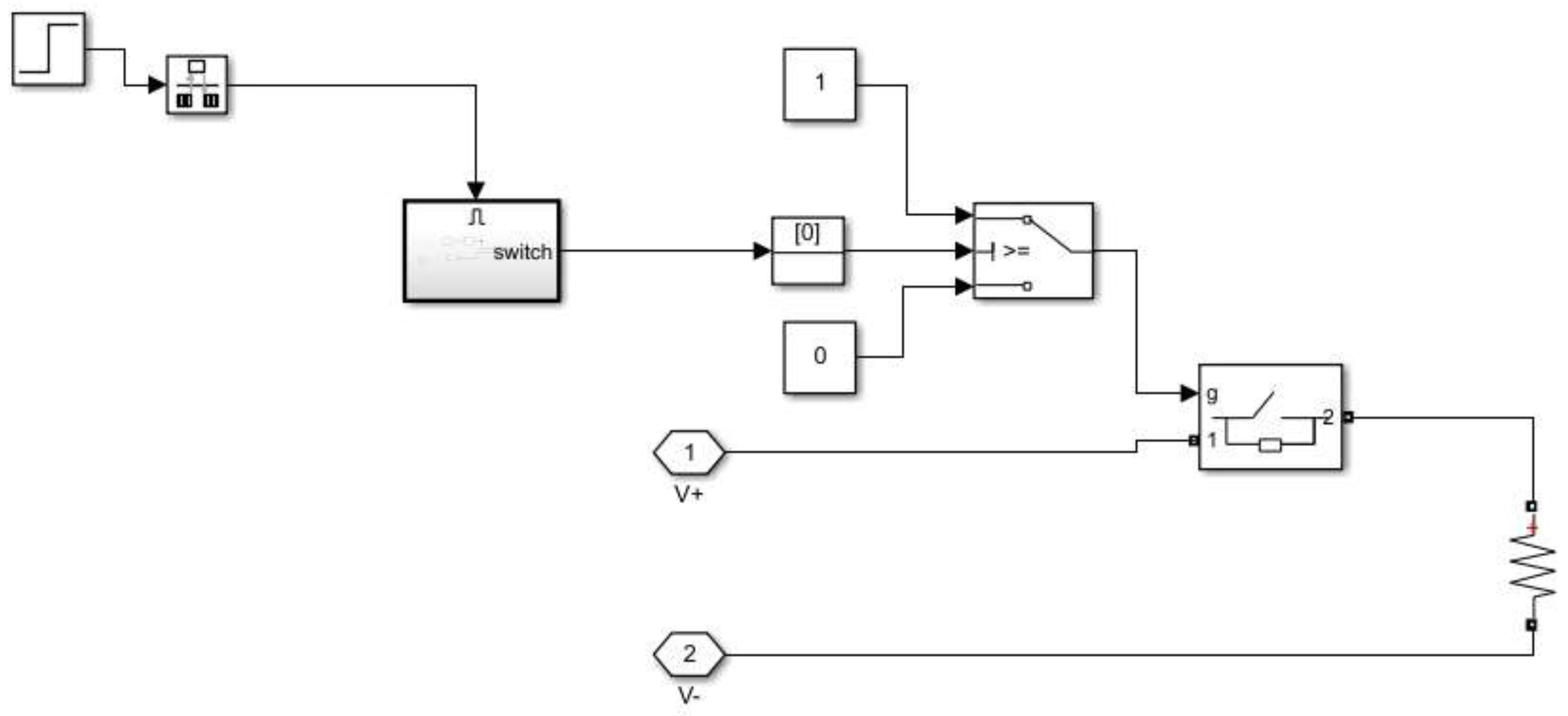
Figure 6.
Photovoltaic microgrid simulation model.
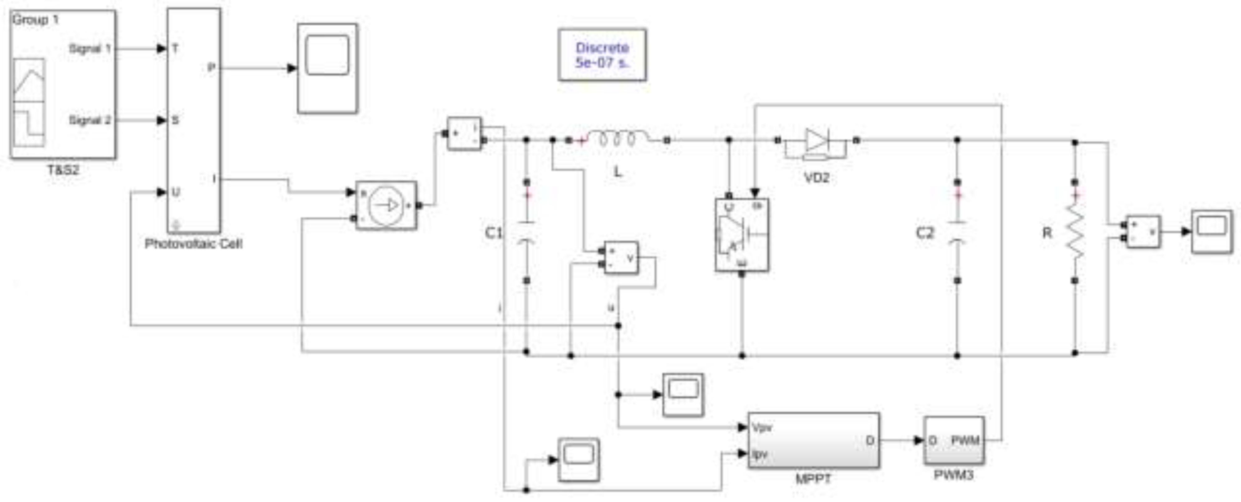
Figure 7.
Simulation environment parameters.
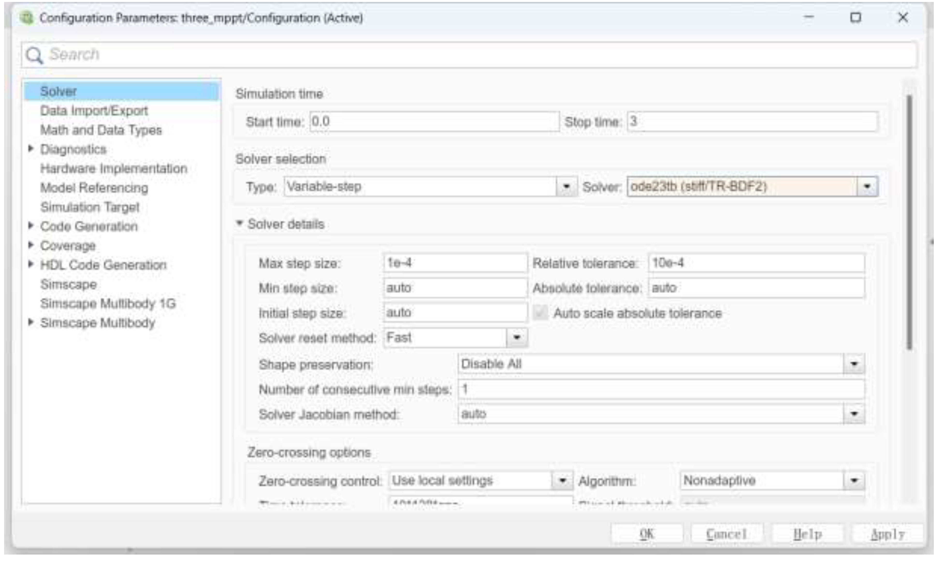
Figure 8.
P-V characteristic curve of photovoltaic array.
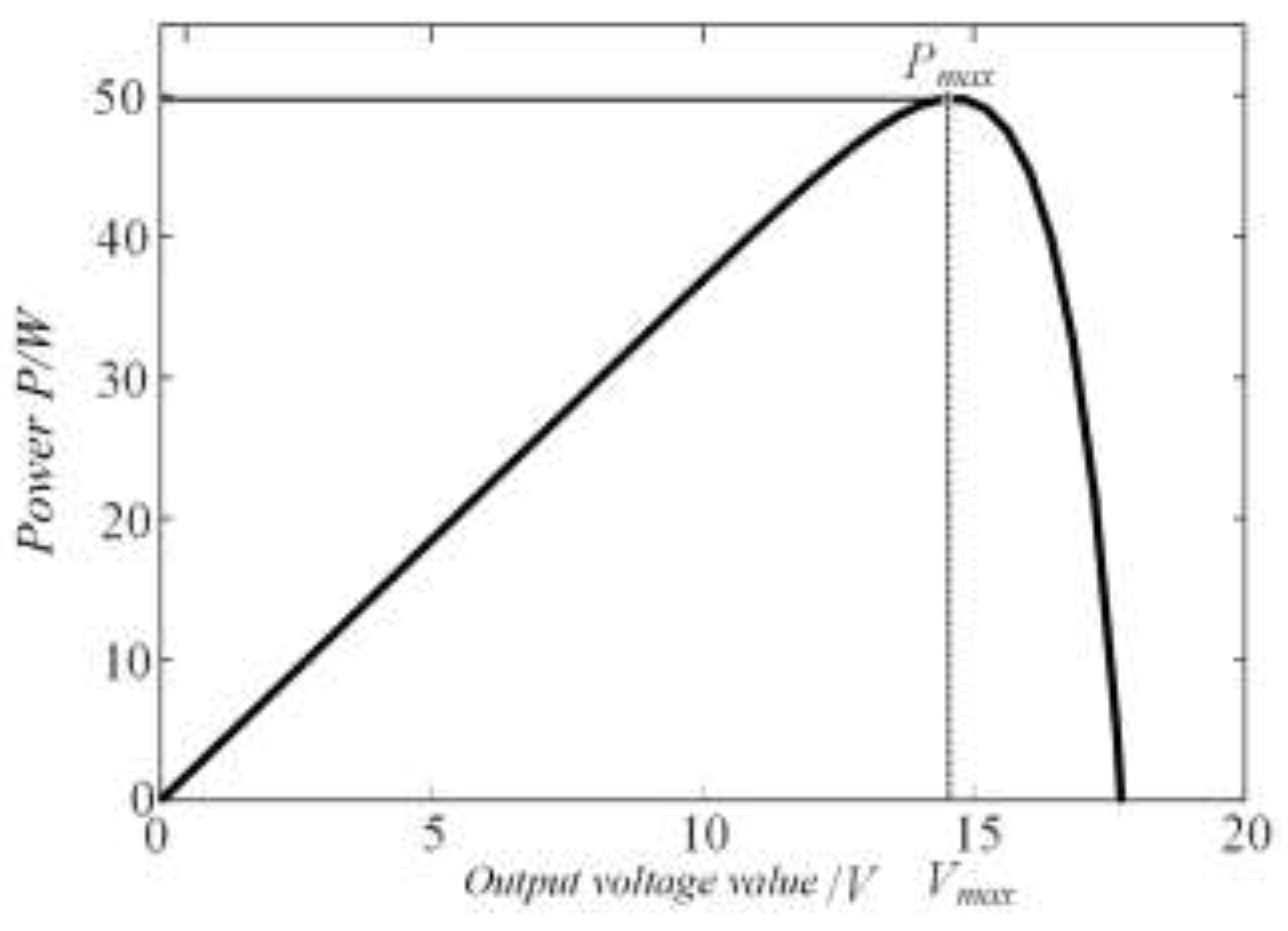
Figure 9.
I/U and P/U characteristic curves of different light intensities at the same temperature.
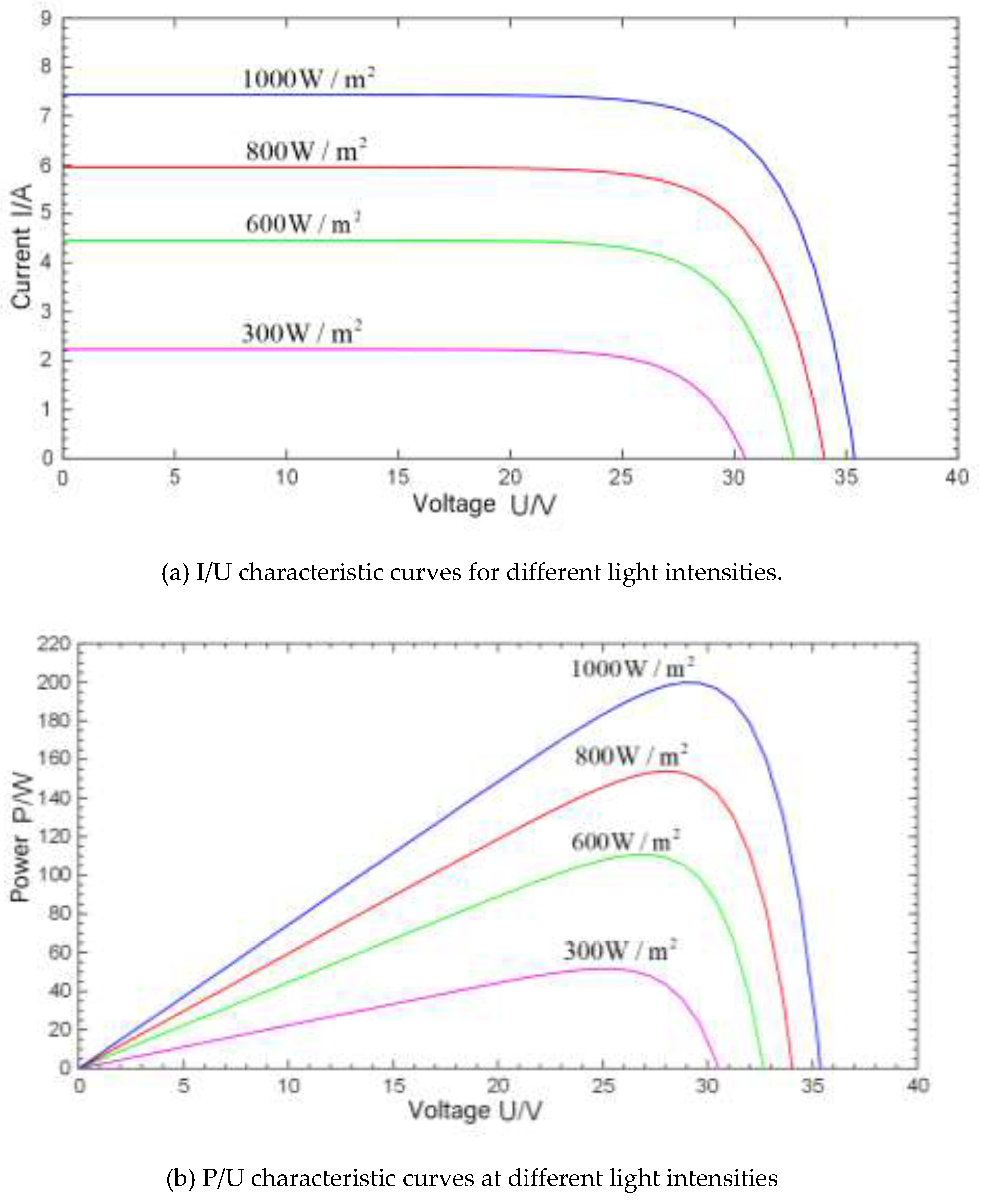
Figure 10.
I/U and P/U characteristic curves of different light intensities at the same temperature.
Figure 10.
I/U and P/U characteristic curves of different light intensities at the same temperature.
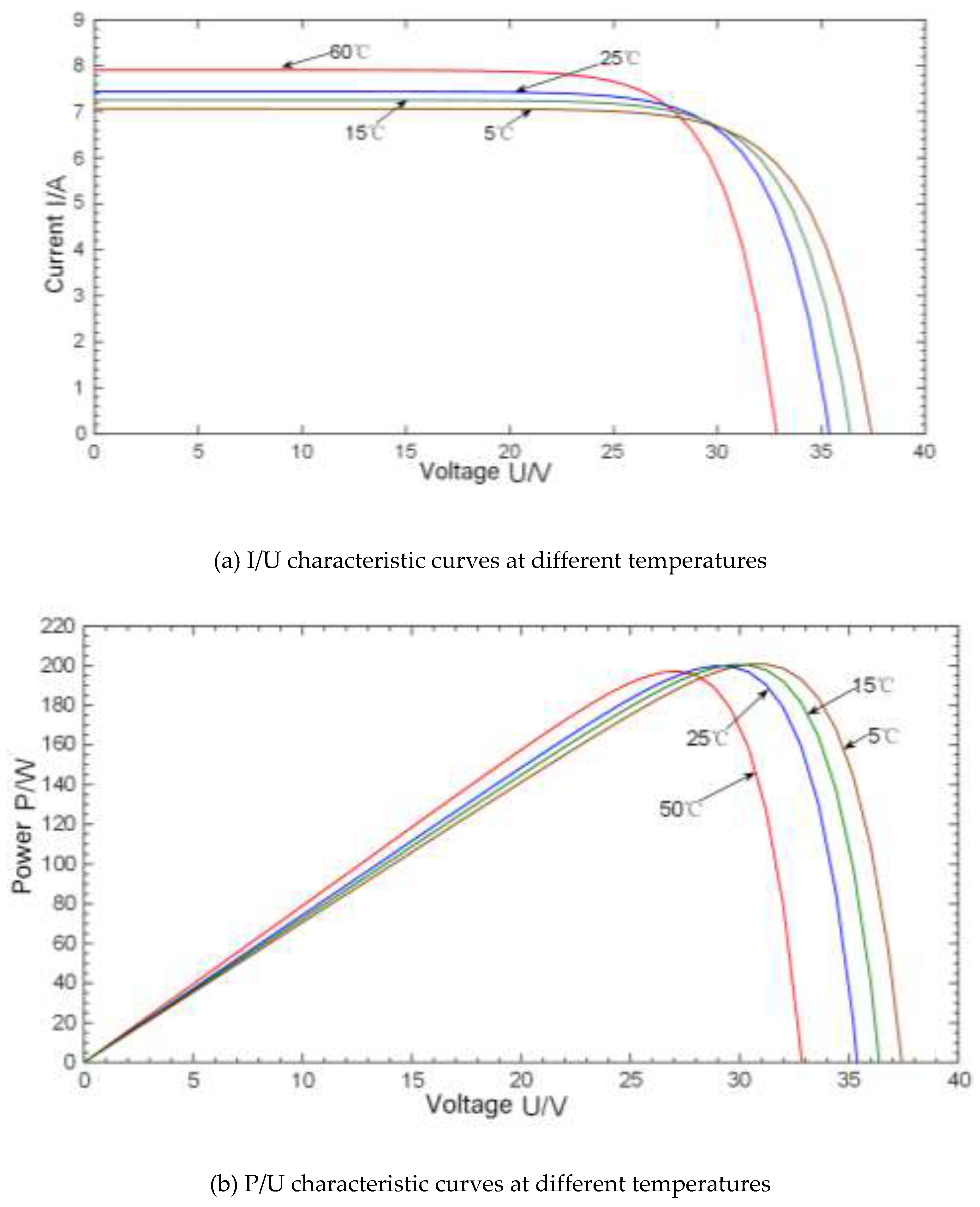
Figure 11.
Maximum output algorithm control structure.
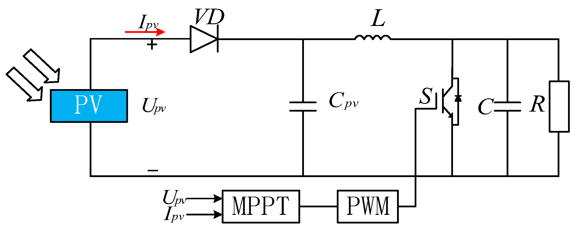
Figure 12.
Operation principle of incremental conductance method.
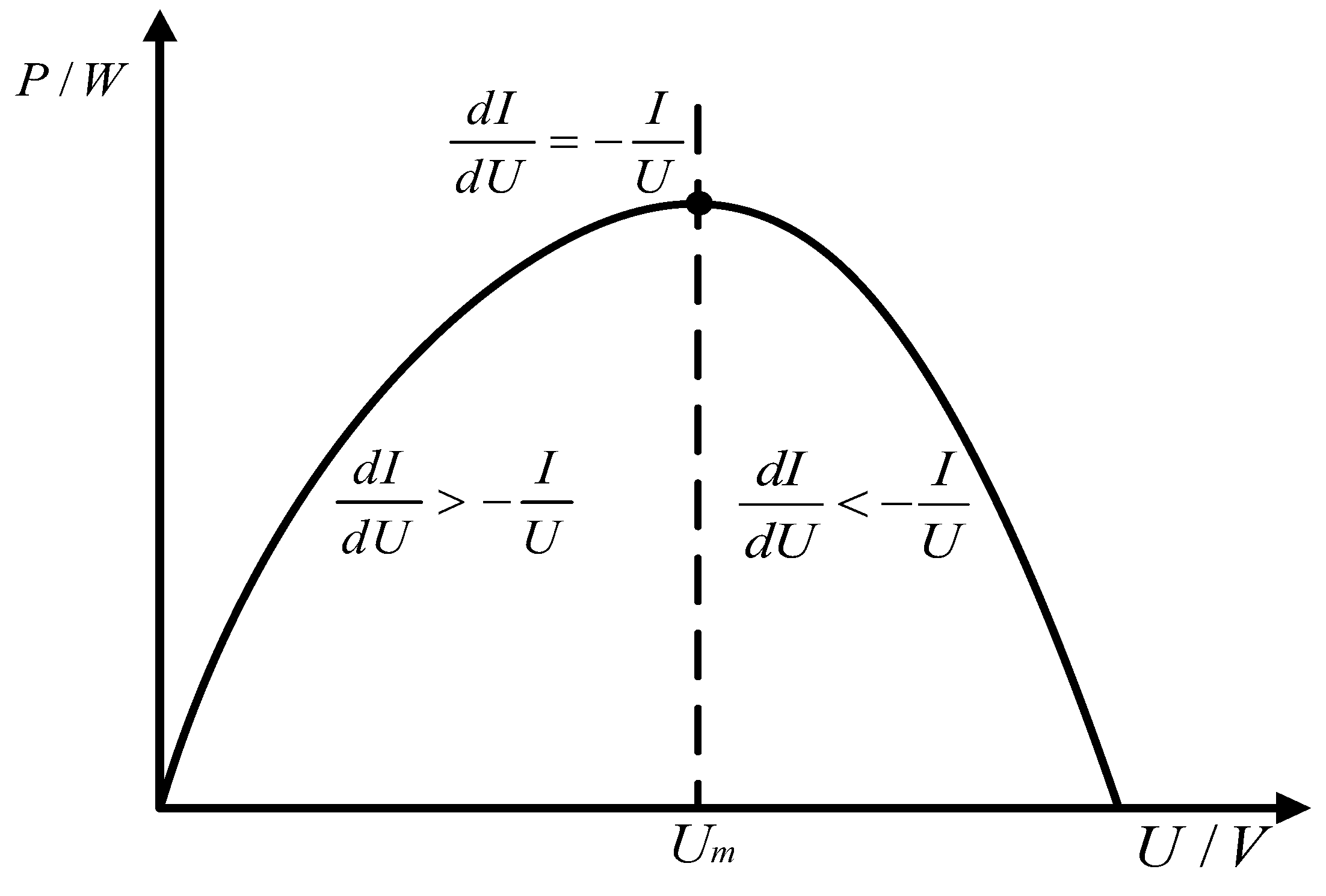
Figure 13.
Incremental conductance control flow.
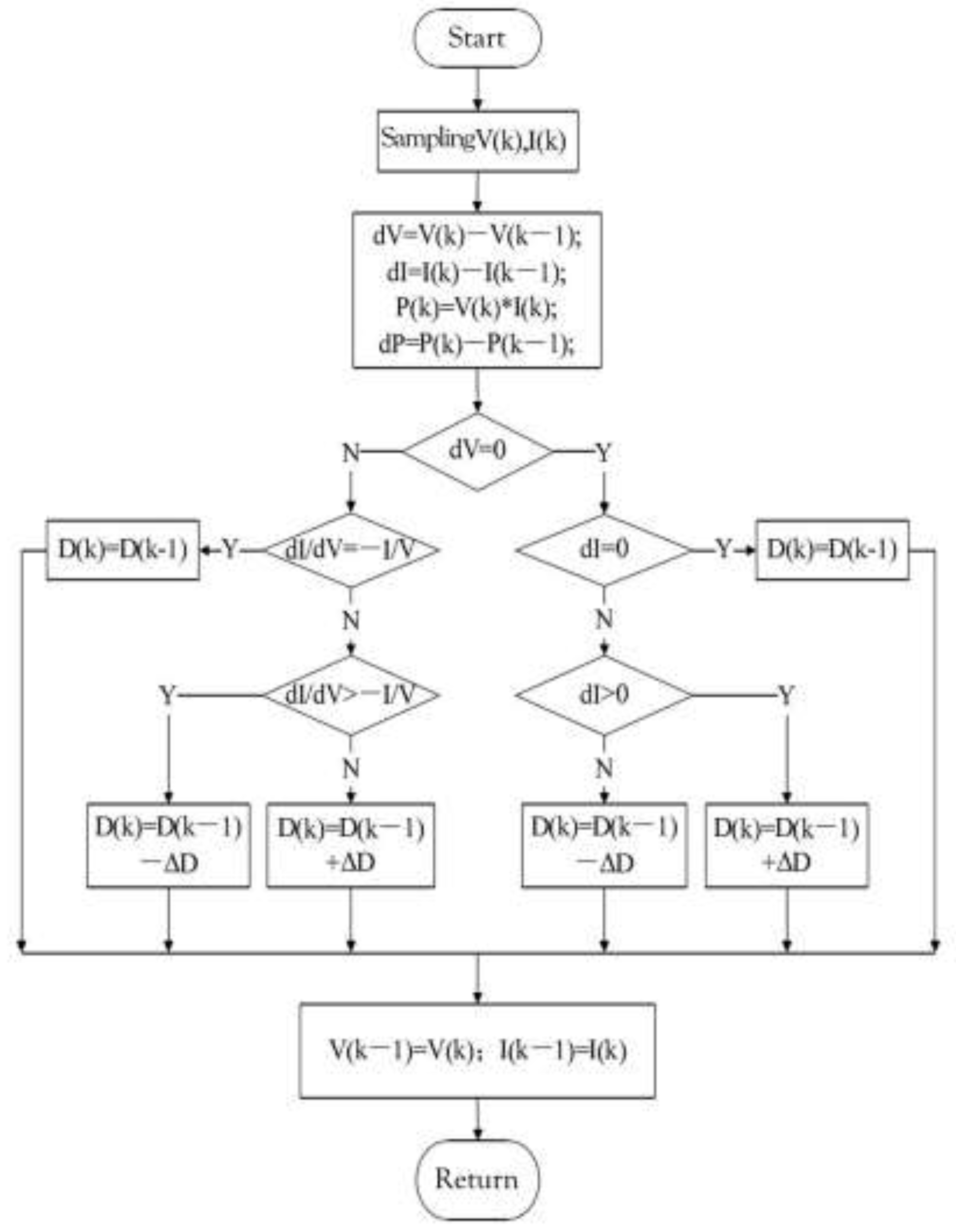
Figure 14.
Incremental conductance simulation module.
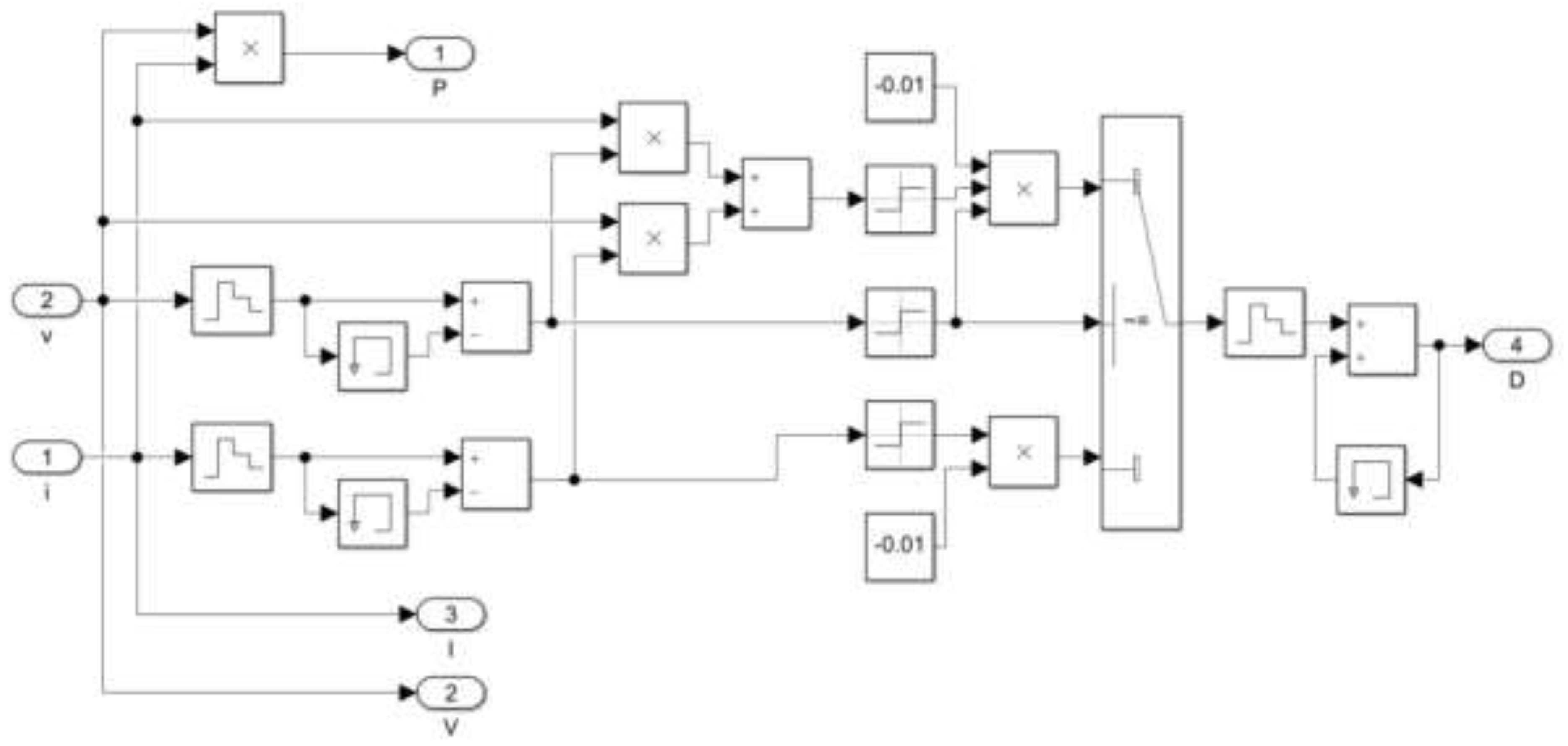
Figure 15.
Duty cycle control structure.
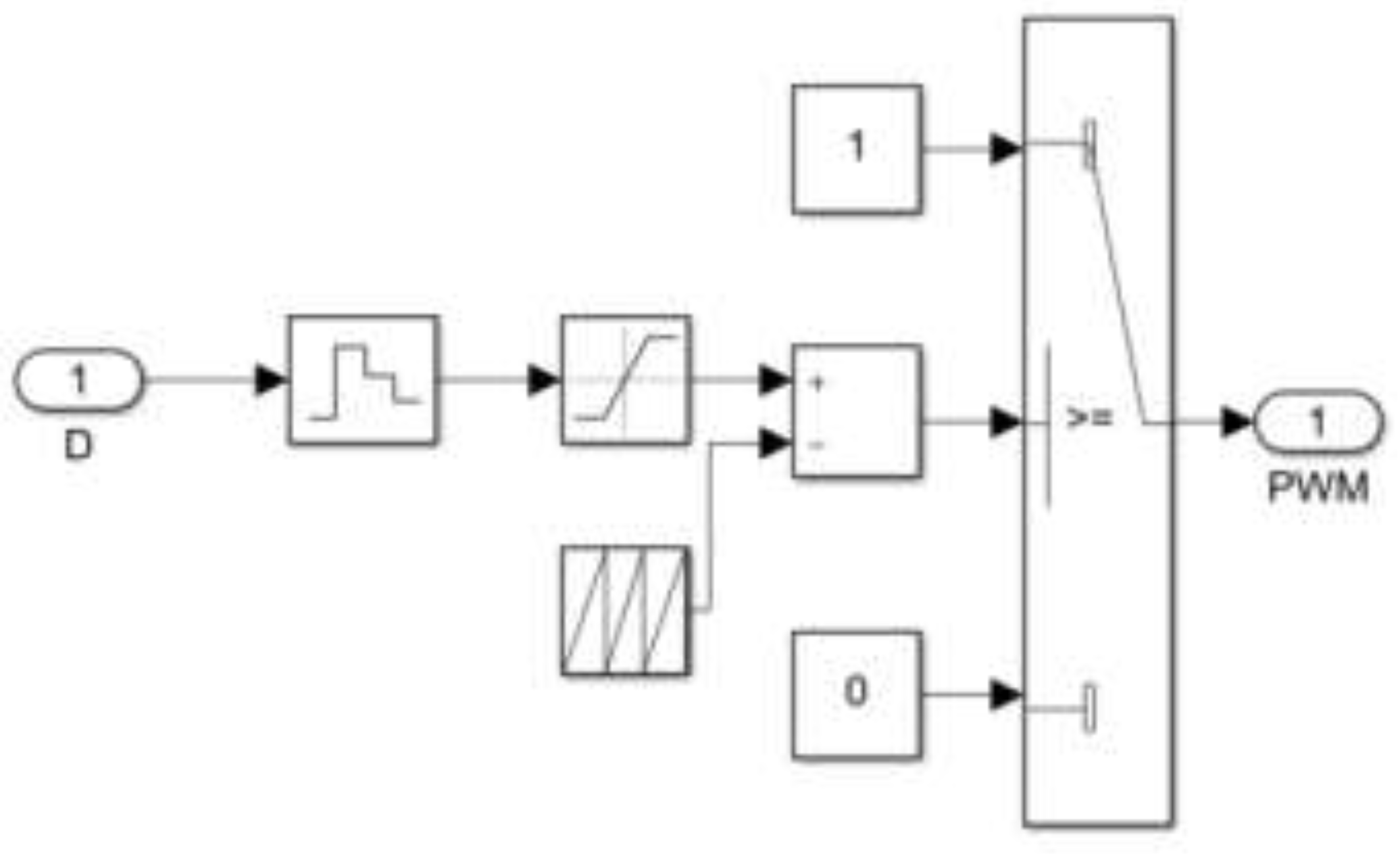
Figure 16.
Light intensity curve.
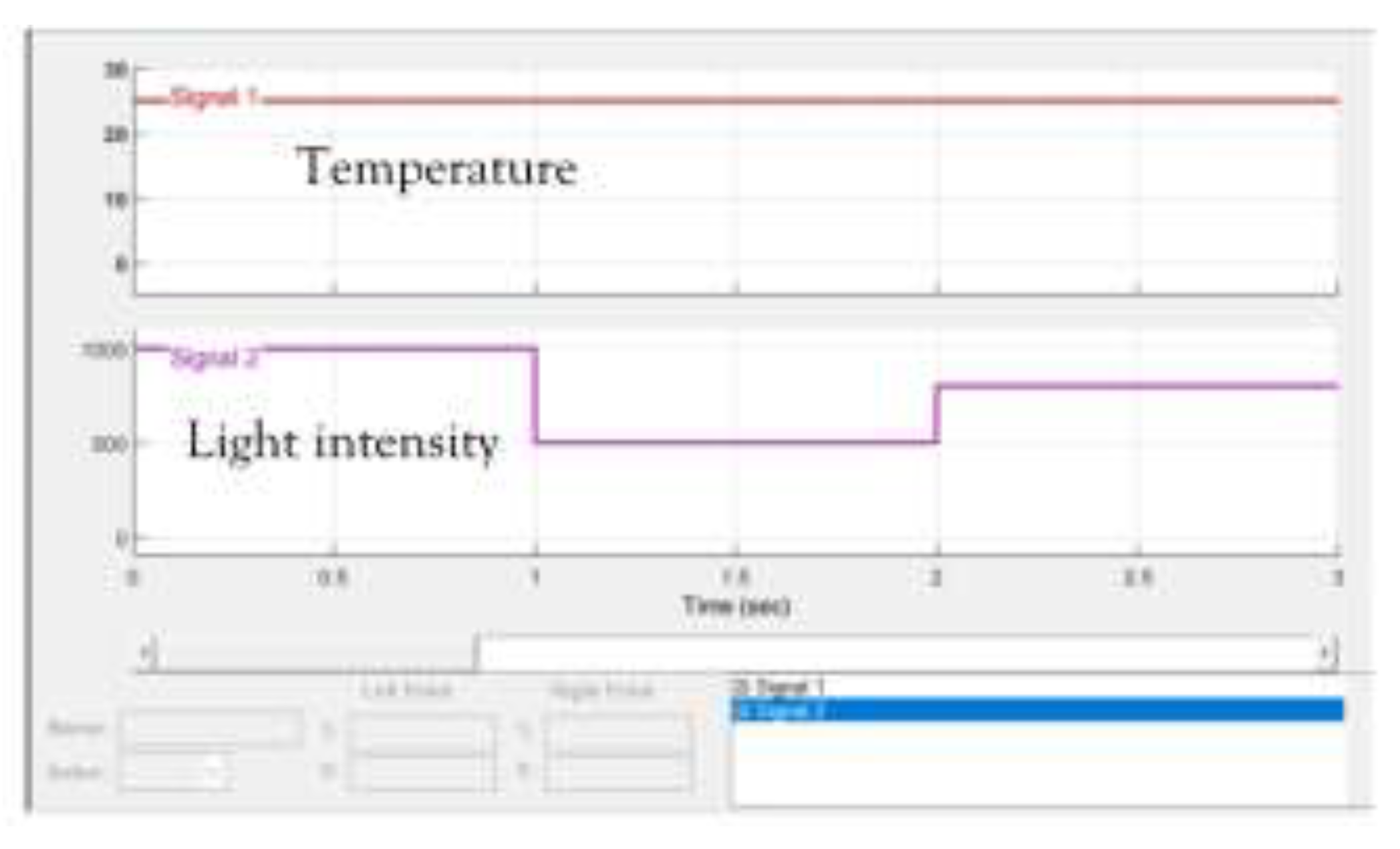
Figure 17.
PV array output curve under different light intensities.
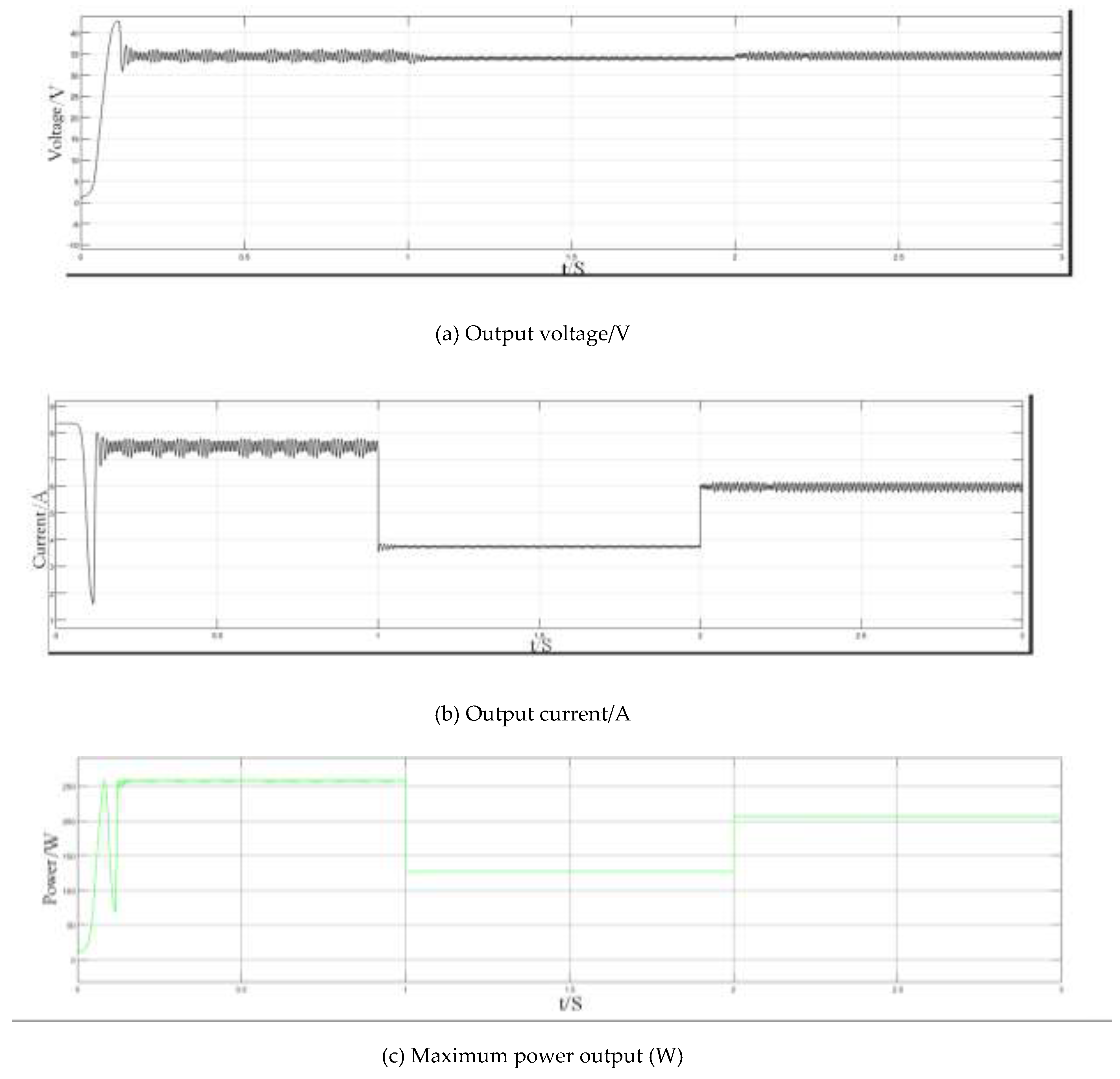
Figure 18.
Light intensity curve.
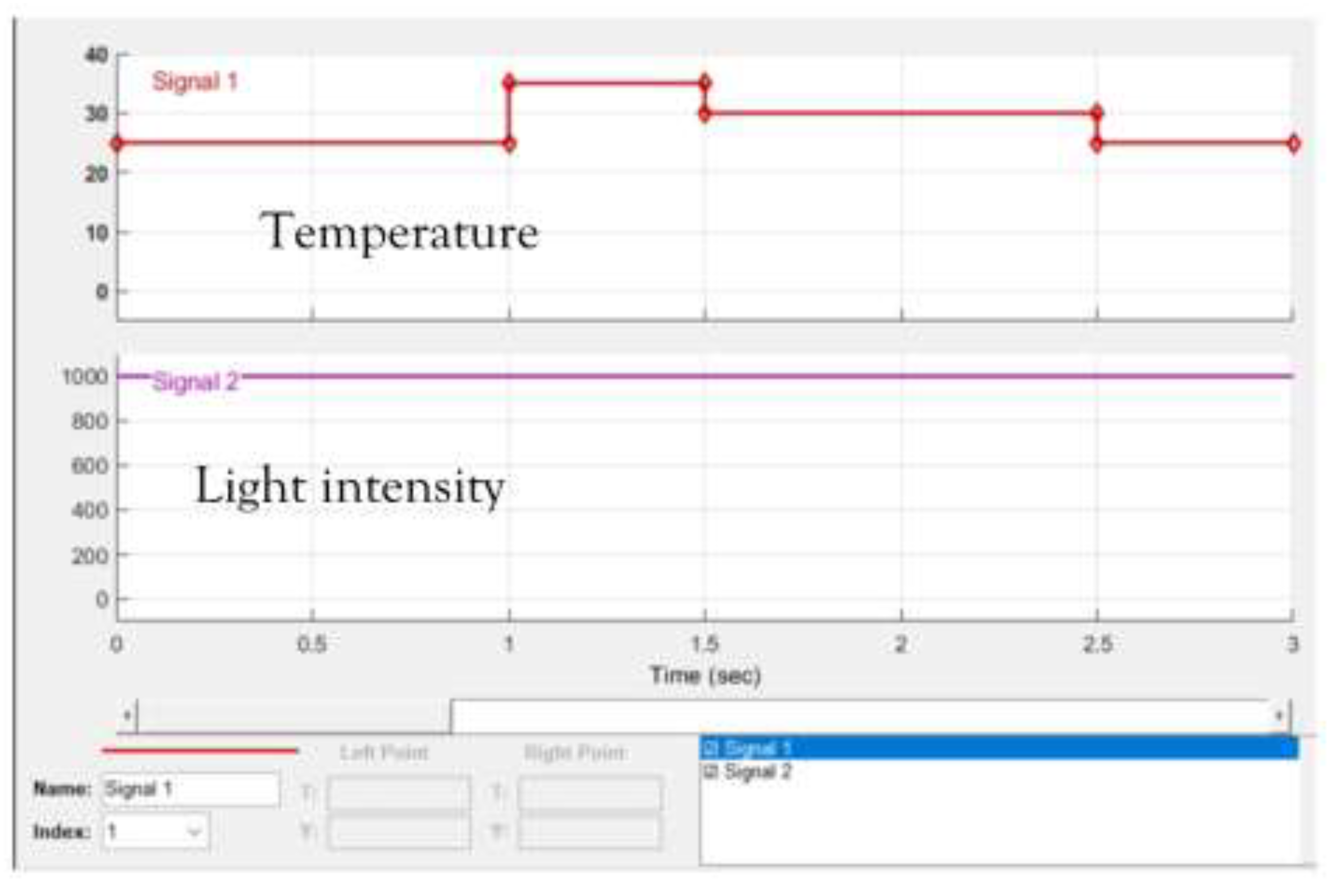
Figure 19.
PV array output curve under different light intensities.
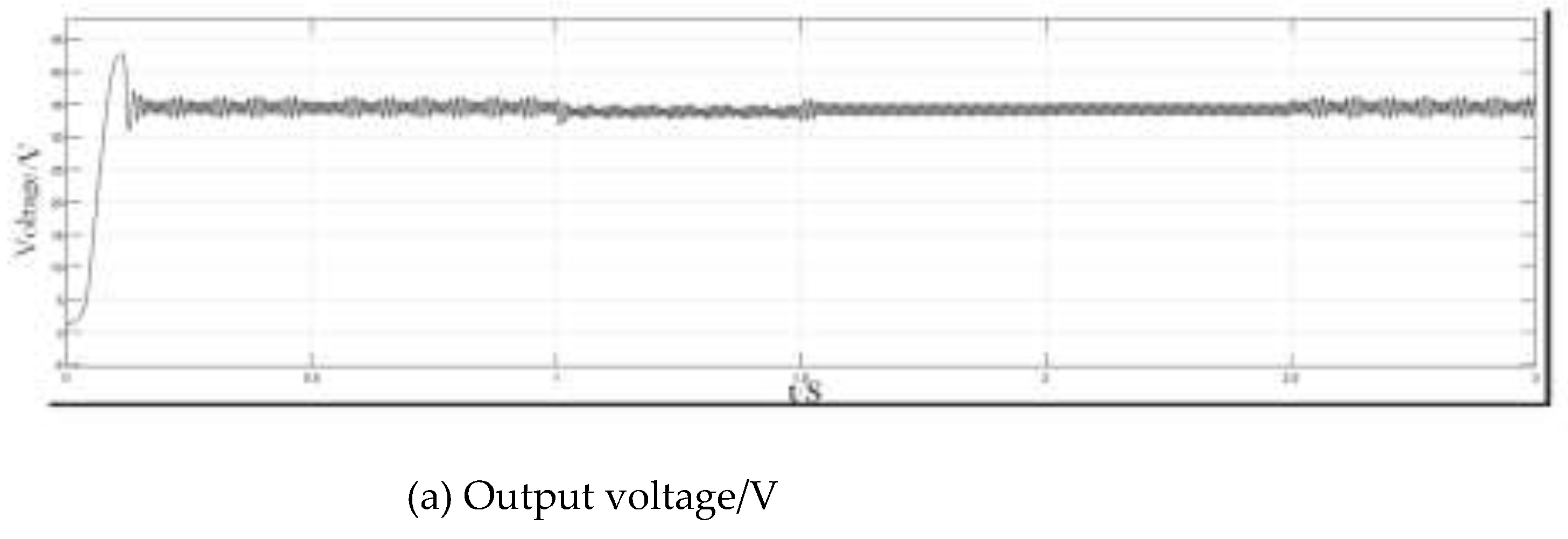
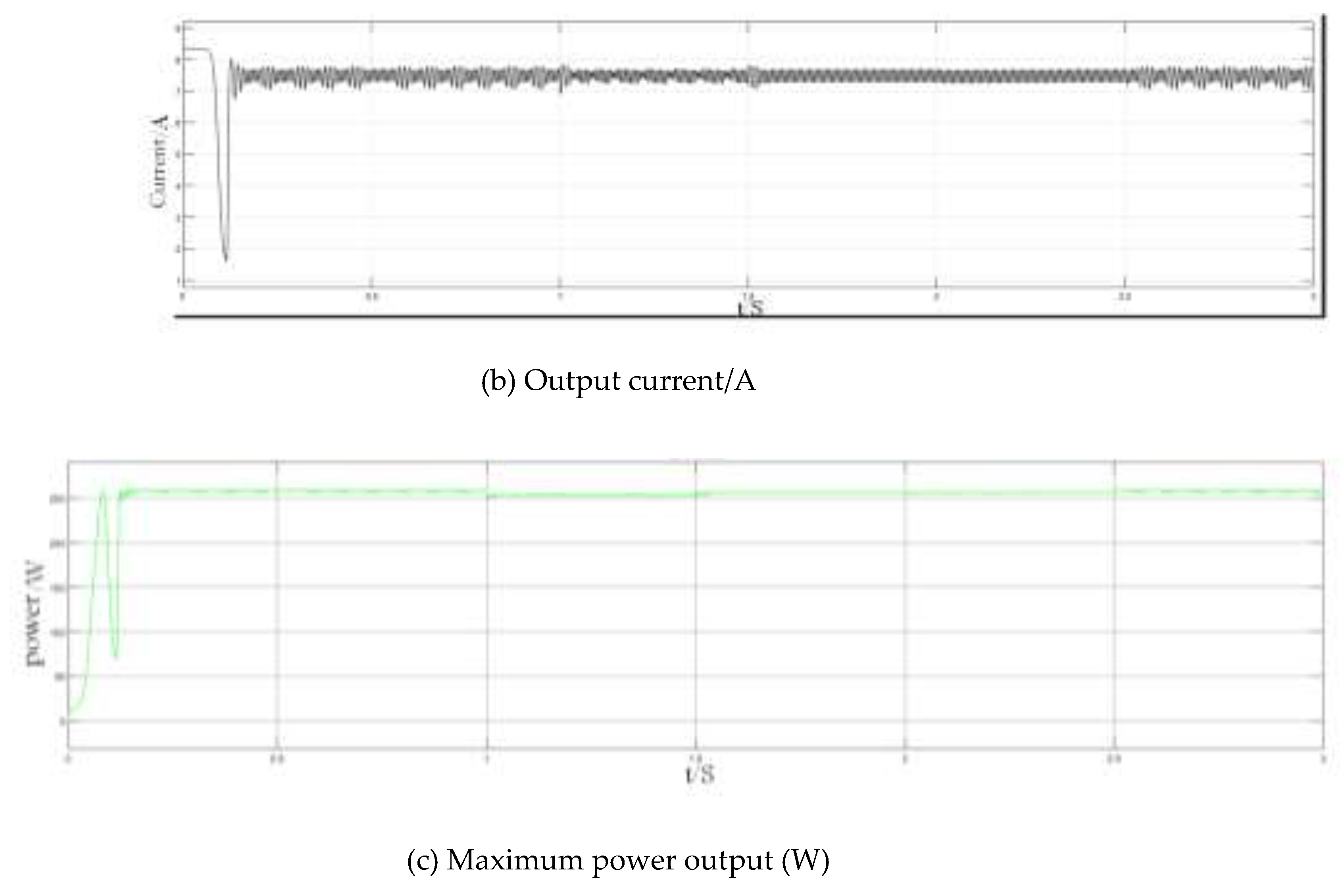

Table 1.
Model parameter.
| Name | Numerical Value |
|---|---|
| Stabilivolt capacitor in photovoltaic side/F | 20e-5 |
| Filter inductance in photovoltaic side/H | 300e-6 |
| DC load/Ω | 30 |
| Capacitor in load side/F | 100e-6 |
Table 2.
PV panel parameters.
| Name | Values |
|---|---|
| Short-circuit current/Isc | 8.35A |
| Open circuit voltage/Usc | 43.6V |
| Maximum power point voltage/Um | 34.5V |
| Maximum power point current/Im | 7.5A |
| Maximum power point power/Pm | 258.75W |
Disclaimer/Publisher’s Note: The statements, opinions and data contained in all publications are solely those of the individual author(s) and contributor(s) and not of MDPI and/or the editor(s). MDPI and/or the editor(s) disclaim responsibility for any injury to people or property resulting from any ideas, methods, instructions or products referred to in the content. |
© 2024 by the authors. Licensee MDPI, Basel, Switzerland. This article is an open access article distributed under the terms and conditions of the Creative Commons Attribution (CC BY) license (http://creativecommons.org/licenses/by/4.0/).
Copyright: This open access article is published under a Creative Commons CC BY 4.0 license, which permit the free download, distribution, and reuse, provided that the author and preprint are cited in any reuse.


