
Submitted:
21 October 2025
Posted:
22 October 2025
You are already at the latest version
Abstract
Accumulation of salts in irrigated soils can be detrimental not only to growing crops but also to groundwater quality. Soil salinity should be monitored reg-ularly and appropriate irrigation with the required leaching rate should be applied to avoid excessive salt accumulation in the root zone, thereby im-proving soil fertility and crop production. We combined two frequency domain electromagnetic induction (FD-EMI) mono-channel sensors (EM31 and EM38) and operated them at different heights and with different coil orientations to monitor the vertical distribution of soil salinity in a salt-affected irrigated area in Kairouan (central Tunisia). Multiple measurement heights and coil orientations were used to enhance depth sensitivity and thereby improve salinity predictions from this type of proximal sensors. The resulting mul-ti-configuration FD-EMI datasets were used to derive soil salinity information using inverse modeling based on a recently developed in-house laterally constrained inversion (LCI) approach. The collected apparent electrical con-ductivity (ECa) data were inverted to predict the spatial and temporal distri-bution of soil salinity. The results highlight several findings about the distri-bution of salinity in relation to different irrigation systems using brackish water, both in the short and long term. The expected transfer of salinity from the surface to deeper layers was systematically observed by our FD-EMI surveys. However, the intensity and spatial distribution of soil salinity varied between different crops, depending on the frequency and amount of drip or sprinkler irrigation. Furthermore, our results show that the vertical transfer of salinity is also influenced by the wet or dry season. The study provides in-sights into the effectiveness of combining two different FD-EMI sensors EM31 and EM38 for the monitoring of soil salinity in agricultural areas, contributing to the sustainability of irrigated agricultural production. The inversion ap-proach provides a more detailed representation of the of soil salinity distri-bution over spatial and temporal scales across different depths and irrigation systems compared to the classical method based on soil samples and labora-tory analysis which is a point-scale measurement. It provides a more extensive assessment of soil conditions at depths up to 4 m with different irrigation systems. For example, the influence of local drip irrigation was imaged and the history of a non-irrigated plot was evaluated, confirming the potential of this method.
Keywords:
soil salinity
; electromagnetic induction
; inverse modeling
; geophysical survey design
; Tunisia
1. Introduction
Approximately 833 million hectares of land worldwide are considered to be affected by salinization [1]. These affected areas are located in arid and semi-arid regions, which are characterized by high evaporation and water scarcity. Soil salinization is a threat to agricultural productivity and food security. In Tunisia, soils affected by salt are around 1.5 million hectares, which correspond to about 10% of the country area [2]. Tunisia's total agricultural production has already decreased by 12% between 2000 and 2017 due to the effects of climate change, namely drought and water scarcity [3]. In addition, high temperatures exacerbate soil degradation by increasing erosion rates and reducing soil moisture, which can lead to reduced crop yields and food availability. This problem is expected to intensify due to several factors, including low rainfall, high evaporation rates and the use of saline water in irrigation [4].
In arid and semi-arid regions, climate change increases the occurrence of extreme weather events, such as floods and droughts. These events not only disturb the natural water cycle but also increase the risks of soil and groundwater salinization, which is a significant concern for agricultural systems and water quality. Imaizumi et al. [5] highlighted the link between salt movement and groundwater flow, with salts being leached away during the rainy season. However, this salt leaching is being increasingly disrupted by the combined effects of climate change and human activities. When groundwater is withdrawn excessively, aquifers become depleted, leading to higher salt concentrations creating a feedback loop: water over-extraction contributes to soil salinization, which in turn reduces water availability and fertility. This poses a serious threat to the sustainability of agricultural practices. Soil salinity has a major impact on the environment through increased erosion of the ecosystem including reduction of vegetation cover, decrease in soil fertility, decrease in organic matter and organic carbon stock, increase in pH value, reduction of crop yield [6,7].
Salts are highly soluble and can be transported by surface water and groundwater. There are two types of salinity, those that occur naturally in soils and those that are caused by human activities. The latter is a growing concern because its spatial and temporal variability makes it difficult to manage [8]. Modern irrigation, such as drip irrigation, has added complexity to how salinity is distributed in the root zone [9]. In this case, long-term salinity management is therefore becoming more difficult [10]. In this context, accurate spatial data on salinity levels in the root zone is crucial. This information helps optimizing water resources, manage salinity, and assess the impact of climate change on soil and water quality [10]. Traditional soil mapping methods, which rely on field surveys and sample collection, are not always sufficient to provide timely the information needed to manage salinity [11,12]. These methods, while valuable, are costly and time-consuming. Moreover, they cannot provide the high spatial and temporal resolution required on a large scale [13]. As a result, there is a growing need for more efficient and accurate methods.
One promising solution is the use of efficient non-invasive geophysical methods, which have been applied to various agricultural problematic [14,15,16,17]. The frequency domain electromagnetic induction (FD-EMI) method can provide details about soil electrical conductivity profiles from the surface to different depths. FD-EMI instruments are particularly useful for mapping variations in soil properties across different spatial scales due to their reliability, speed, and non-destructive nature [18,19]. Multi-frequency or multi-coil FD-EMI instruments allow for simultaneous sampling at multiple depths, enabling both vertical and horizontal distributions of soil conductivity to be assessed [20,21,22]. This technique also allows creating detailed maps of soil properties such as texture, moisture content, cation exchange capacity, and salinity [23,24,25]. By sensing the electrical conductivity distribution in the subsurface, FD-EMI sensors can detect spatial salinity patterns [26]. However, interpreting the data can be challenging, as electrical conductivity is controlled by several soil properties, including porosity, pore fluid composition, and soil matrix components [27]. Factors like FD-EMI transmitter frequency, coil separation, and soil conductivity influence the depth of penetration and the accuracy of the data [28,29]. By being sensitive to the pore fluid conductivity, which increases with salt concentration, these tools offer relatively accurate and timely salinity data, which can support precision agriculture and sustainable land management.
Procedures to estimate the vertical distribution of soil salinity are based on the inverse modeling of FD-EMI data [30]. This technique uses algorithms to convert observed FD-EMI apparent electrical conductivity (ECa) data as defined in McNeil [31] into heterogeneous subsurface models of electrical conductivity, allowing for the creation of multi-dimensional maps of salinity distribution (1D, 2D, 3D). This provides insights into soil salinity and its distribution in the root zone. In addition, quantitative interpretation with inversion software can provide detailed salinity maps at various depths [32]. Selim et al. [33] inverted multi-height ECa data acquired with a single channel FD-EMI sensor (CMD2) in a salt-affected irrigated area located in Egypt. Their inversion procedure generated electrical conductivity images up to a depth of 90 cm to predict the temporal and spatial soil salinity distribution. Similarly, De Carlo and Farzamian al. [34] used ECa data collected from a multi-configuration sensor (CMD-Mini-Explorer) in a cultivated crop in southern Italy in order to produce a detailed soil salinity distribution up to a depth of 1m. In another study, Farzamian et al. [35] employed ECa data collected from a single channel sensor (EM38) sensor placed at several heights above ground and operated with several orientations across an agricultural area of Fatnassa Saharan oasis (southern Tunisia) using a spatially constrained 1D layered medium inversion algorithm (pseudo-3D) to characterize the spatial distribution of soil salinity. In our study, we combined ECa data from two single channel sensors (EM38 and EM31). Each of them was operated at different heights and with different coil orientations to generate 50 m profiles of soil salinity to a depth of 4 m. A pseudo-2D inversion approach based on laterally constrained 1D inversion (1D LCI) was applied to this 50 m profiles in order to characterize the lateral and vertical distribution of soil salinity and to assess the transfer of salt into deeper soil layers.
This study was conducted at 5 sites along a 4 km transect in the Merguelil irrigated perimeter in the Kairouan governorate, in the central region of Tunisia. The Merguelil site is an example of a regional scale salinity assessment due to its elevated soil salinity. The study area is characterized by a semi-arid climate where irrigation and climate change have led to increased salinity. The objectives of the study were to:
- Determine the transfer of salts from the topsoil to deeper layers by coupling the measurements of two different FD-EMI sensors (EM38 and EM31, Geonics Ltd).
- Assess the capabilities and reliability of these two devices for the detection and characterization of soil salinity by interpreting the multi-depth ECa datasets with quantitative inverse modeling methods.
- Evaluate the effect of irrigation systems (e.g., drip and sprinkler) and type of crop on the soil salinity.
- Reveal temporal variation in soil salinity using time-lapse FD-EMI surveys.
2. Materials and Methods
2.1. Study Area
The Kairouan Plain is located in central Tunisia. This basin is filled with over 700 meters of Pliocene-Quaternary detrital sediments that were carried down from the Tunisian Mountains by numerous rivers. The most important of these rivers are the Zeroud and the Merguellil. The region has a semi-arid climate, with an average annual rainfall of 300 millimeters. The average temperature is 19.6°C, and the Penman potential evapotranspiration rate is nearly 1,600 mm per year. The groundwater table of the Kairouan Plain is the largest in central Tunisia. It is notable for its 3,000 km² extent. For over 50 years, the plain has been subject to heavy human intervention and overexploitation for irrigation and drinking water needs. Significant human interventions include the construction of large dams on the Zeroud River in 1982 and the Merguellil River in 1989. The soils have variable textures and consist of alternating layers of sandy clay, gravel, and detrital elements with varying clay content. The present study was performed at five different parcels along the transect T4 from which is located in the irrigated perimeter of Merguelil (Figure 1). The Merguelil irrigated perimeter span across a surface of 2000 hectares and is located 7 km downstream from the dam at an altitude of 170 meters.
These five different plots were identified to represent the overall variability in crop type in term of plant species and irrigation status (see Figure 1). At the plot level, six profile lines of 50 m length were selected by maximizing their distance from potential sources of disturbance for the FD-EMI measurements (e.g., metallic objects).Although the main initial goal was to estimate the depth distribution of soil salinity, we nevertheless perform densely sampled (1 m station spacing) FD-EMI profiles to detect lateral variations, which may be critical for our interpretation. The two first profiles (S1 and S2) are located in the plot A (Figure 1), which covers 1.5 ha and contain 165 olive trees with 10 m x10 m spacing. This plot has a rectangular shape in the southern part and a trapezoidal shape in the northern part, where there are 21 almond trees between the olive trees. The olive trees are 23 years old, and the almond trees are 10 years old. Surface irrigation in plot A consists in supplementary drip irrigation with a rate of 1-3 times per month depending on the dryness condition, which is typically the most severe in August. The total irrigation volume in plot A ranges between 500 m3 and 1000 m3, depending on climatic conditions. No irrigation occurs in November because of harvesting activities.
The third profile (S3) is located in the plot B, which covers 1.7 ha. Plot B was left fallow from 2019 until the start of our investigation in November 2023 (4 years). At the time of our survey, this plot appeared to be homogeneous and uniform. However, historical aerial photography indicates that this profile crossed two distinct parcels. The first parcel corresponds to a non-irrigated area while the second parcel was subjected to residual irrigation (sometimes ploughed and cropped). The fourth profile (S4) was performed on plot C (1.7 ha), which is used for cereal culture. It is irrigated by sprinkler every 10 to 18 days for 18 hours (421 m³ per ha). Nineteen sprinklers, spaced approximately 10 m apart, were used for this irrigation. Two additional profiles (S5 and S6) were performed on Plot D and E, respectively. S5 one was placed in plot D between rows of young almond trees (1.5 years old) spaced with a distance of 6 m x4 m over an area of 1.25 ha with a total of 500 trees. These young almond trees are watered twice a week by drip irrigation. It should be noted that this plot was used for annual crops before it was planted with almonds.S6 was laid between rows of young olive trees (1.5 years old) at 6 m x4 m spacing for an area of 1.25 ha, with a total of 500 trees. These young olive trees are watered twice a week by drip irrigation.
2.2. Devices Used for ECa Measurements
We used loop-loop FD-EMI instruments to sense the electrical conductivity of the subsurface. The loop-loop FD-EMI method consists in generating a time-varying “primary” magnetic field with the transmitter coil, which interacts with the nearby conductive subsurface by causing eddy current. This subsurface eddy currentis in turn associated to a secondary magnetic field to be measured by the receiver coil(s). The intensity and dynamics of the eddy current (and thereby its secondary magnetic field) is controlled by the distribution of electrical conductivity within the subsurface. Loop-loop FD-EMI data are typically provided in term of ratio of the primary field (H_p) to the secondary field (H_s), which can be converted into an apparent electrical conductivity (ECa) using the method provided by McNeill [31] although the robustness of this linear transformation is affected by the coil spacing, orientation, device height, frequency and magnetic susceptibility [36,37].
Among the wide variety of loop-loop FD-EMI devices, the EM38 sensor (Geonics Ltd) is particularly useful for agricultural studies because its sensing depth is aligned with the root zone (1.0 m to 1.5 m), allowing for the assessment of variations in soil salinity near the surface that affect crops [28,38]. The EM38 sensor is relatively easy to handle due to its small size (1 m) making it suitable to efficient hand-held surveying. It is designed with a transmitter and receiver coil placed 1.0 m apart at each end of a non-conducting rod and operates with a monochromatic 14.5 kHz transmitter coil.
The EM31 sensor (also from Geonics Ltd) operates with a monochromatic transmitter signal of9.8 kHz and has a coil spacing of 3.66 m, giving an apparent electrical conductivity measurement averaging up to a depth of approximately 6.0 m with horizontal co-planar (HCP) coil geometry and 3.0 m with vertical co-planar (VCP) geometry [39]. Both devices provide a low induction number apparent conductivity LIN ECa [31], which have been computed from the magnetic field ratio assuming a zero height, a homogenous medium, and a low frequency setting (i.e., skin depth of the eddy current much larger than the coil distance). Because both devices are single-channel sensors (one transmitter frequency and one receiver coil), the only way to measure with varying depth of investigation is to combine their data, and/or to change the height above ground, and/or to change the orientation of the coils.
Accordingly, we combine measurements from the EM38 and EM31 at different height and in both HCP and VCP geometries in order to perform multi-depth FD-EMI soundings (Figure 2). In theory, this approach can improve the resolution and robustness of the inverse modeling, which is used to image the vertical distribution of soil salinity.
2.3. Procedure of Data Acquisition
LIN ECa data were collected along each of the six 50-meter profiles in November 2023 (dry season). This survey was repeated only for S1 (adult olives) in April 2024 (wet season) in order to determine the influence of adult olives on ECa, as olive crops are generally of primary importance in Tunisia. The EM38 and EM31 were placed at different heights from the ground and kept in the same direction. This procedure was carried out using a plastic container (Figure 2). Care was taken to ensure that no metal parts were present in the lateral footprint of the FD-EMI soundings (i.e., within a distance of 6 m from the profiles. For each profile, 51 points spaced 1 m apart were determined, at which the ECa measurements were collected in both horizontal and vertical modes and at different heights above ground (Figure 2).
This systematic approach allows for tracking changes in soil salinity characteristics across the different sites, while maintaining a uniform methodology for each profile. The high density of data points provides robust insights into the vertical and lateral distribution of soil salinity.
Number of Measurements Recovered
For the six profiles, ECa measurements were performed at three heights (0 m, 0.3 m, and 0.9 m) above the ground for both HCP and VCP modes. The total number of measurements was calculated as follows:
Total Measurements=6(profiles) ×50 (positions in the profile length) ×2 (coil modes) ×3 (heights) = 1800 data (corresponding to 300 measurements per profiles)
2.4. Soil Sampling
Nineteen sampling sites have been identified because of their relatively high ECa in the six profiles, with 2 to 6 boreholes per profile. At each borehole location, six soil samples were collected from the superficial layer to depths of 120 cm using hand auger. The following levels of soil layers were topsoil (0–20 cm), subsurface (20–40 m), and the subsoils (40–60 cm), (60-80cm), (80-100 cm) and (100-120 cm). Another borehole was drilled in the adult olive plot, with samples collected at 30 cm intervals from the surface to a depth of 600 cm.
2.4.1. Particle Size Analysis
The particle size of the soil was done using the Robinson pipette method [41] to determine the granulometric proportion of each component (clay, loam and sand).
2.4.2. Soil Moisture
Soil moisture was assessed using the gravimetric method. Soil samples brought back from the study area were weighed and then placed in the oven for 24 hours. The difference between the dry and wet weights was used to calculate soil moisture:
θ_p= 100×(W_w-W_D)/W_D
With θ_(p=): soil moisture content in %, W_w: sample wet weight and W_D: sample dry weight.
2.4.3. Electrical Conductivity of the Paste Soil Extract (ECe)
Samples taken from the six segments to a depth of 120 cm were used to extract the soil saturated paste to determine the electrical conductivity (ECe) in the laboratory. These samples were air dried, then crushed and passed through a 2 mm mesh sieve. A quantity of 250 g was taken from each sample and brought to saturation by the gradual addition of distilled water. The soil solution extracted from each sample was used to determine ECe using a conductivity meter (VWR pHenomenal ® CO 3100L) to quantify the total concentration of soluble salts [42].
2.5. Irrigation Water
Irrigation water is pumped by boreholes from a deep aquifer located around 400 m away. This aquifer is fed by the underground infiltration of water from the El Houareb dam built in 1989, which is located on a fault that does not allow water stacking. A network of pipes carries the water to the plots, which are served by valves at the irrigation hydrants. The water salinity has increased from 1.7 dS/m in 2014 to 2.56 dS/m in 2024 and reached the last three years (2022-2025) 3.53 dS/m. Between 2014 and 2025, the chemical composition of the water shows a notable deterioration marked by a general increase in major ion concentrations, notably chloride (Cl-), sodium (Na⁺), calcium (Ca²⁺) and magnesium (Mg²⁺). Electrical conductivity (EC) has doubled, reflecting the increasing mineralization of the water. The pH is alkaline around 7.5.
2.6. Quantitative Interpretation of FD-EMI Apparent Conductivity Data
The LIN ECa readings of the EM38 and EM31 instruments are internally computed from the magnetic field measured by the receiver coil following an incomplete theory [31]. This conversion provides reliable ECa data only for certain limited conditions like a relatively low electrical conductivity setting (< 0.05 S/m) and for instruments lying on the ground surface (as discussed above, the theory does not account for an air layer between the sensor and the subsurface). Accordingly, this theory is limited for our experiment, which involves multi-height measurements (hence requiring the modeling of the height), and which was performed above a relatively conductive medium. In order to compute robust ECa, from the instruments’ reading, we used the method discussed in Guillemoteau et al. [36], which consists in converting the readings back to magnetic field data computing the ECa using the full theory of a homogeneous half-space, i.e., which is valid for the full range of electrical conductivity and which allows the modeling of the instrument height above ground.
In Figure 3, we show one example of LIN and robust ECa vertical sounding curves for the 6 sites that are considered in this study. By comparing both approaches, we see that the LIN theory systematically underestimates the apparent conductivity for the deepest channels (i.e., the ones recorded with EM 31 sensor). We also see that the LIN theory provides different trend toward depths. This is due to a strong artefact for the channel corresponding to the VCP collected at a height of 0.9 above ground. In this case, the air layer critically affects the LIN ECa reading due to a severe decrease of the secondary magnetic field with height for this coil geometry in particular. This result clearly shows that the LIN ECa reading of the instrument would bias the interpretation of our experimental multi-height and multi-configuration FD-EMI data. As a consequence, the robust ECa value will be considered in the following.
In addition to the analysis of the ECa data, we estimated the true vertical distribution of electrical conductivity through a 1D layered medium inverse modeling of the vertical sounding curves following the LCI approach described in Klose et al. [43]. This approach is particularly relevant for our densely sampled profiles as it uses information of adjacent soundings for stabilizing the ambiguous inverse problem. The principle of this pseudo-2D electrical conductivity imaging approach is illustrated in Figure 4.
For inverting our data, the number of layers Nl in the model space was set to 20 with increasing thickness towards deeper layers up to a depth of 5 m.
3. Results
3.1. Results of Soil Sampling
Soil texture, moisture and salinity were studied as these factors influence FD-EMI measurements. Overall, the results show variability in texture, ranging from a silty clay material between 0 and 60 cm, which lies over a siltier to silty-sandy material between 60 and 120 cm. The material becomes silty clay again between 120 and 360 cm, then transitions to silty-sandy to silty-sandy-clay between 360 cm and 600 cm.
The average moisture content of the soils was around 11% (fresh moisture), with a median close to 10% and an average coefficient of variation of 32% (Table 1). However, there were drier sites (moisture below 10%) when uncultivated and wetter sites (moisture above 15%) when cultivated and irrigated. These low soil moisture values suggest that it could not have a determining effect on the apparent salinity measurements. The mean of ECe was 3.99 dS/m with a median of 3.75 dS/m and a coefficient of variation (CV) of 38% (Table 1). Extreme values ranged from a minimum of 1.71 dS/m to a maximum of 8.92 dS/m. The lower values were found in the surface layers, while the higher values were observed in the deeper layers beyond 60 cm.
A highly significant relationship was established between average ECe and ECa-VCPEM38:
ECe (0-1.2 m) = (0.073* ECa- VCPEM38) + 0.97 with R² = 0.8361
This relatively simple relationship enabled us to define a salinity scale for the shallowest ECa measurements, which we can be used to estimate the salinity in the soil layer between 0 a 0.8 m below surface measurements (Table 2).
3.2. Variability by Land Use and Irrigation Management
In this step, the data analysis was realized for each profile by grouping them by irrigation system management and crops, in order to describe their salinity variation trend (Table 3).
Robuste ECa values vary across the six profiles (S1 to S6) with different land use and water irrigation management systems (Figure 5). For S1 and S2, which correspond to adult olive trees irrigated with a low-frequency drip system at a rate of once or twice per month, the ECa values are lowest (below 0.05 S/m), indicating relatively low salinity levels. In contrast, ECa values increase progressively from S3 to S6. S3 shows more pronounced spatial variability between the non-irrigated area and the residual irrigation area. In the non-irrigated area (the fallow part from 0 m to 20 m), robust ECa values are low to intermediate(less than 0.07 S/m). However, in the residual irrigation area (from x > 20 m in S3), robust ECa values are higher, reaching a maximum of 0.1 S/m. These findings demonstrate the strong influence of irrigation on subsurface salinity dynamics. S4 and S5 correspond to young olive and almond tree plantations with a high-frequency drip system that operates twice per week. The robust ECa values in these areas range from 0.05 to 0.15 S/m, which is higher than the robust ECa values recorded in S1 and S2, where low-frequency drip irrigation is used. The highest ECa values, exceeding 0.18 S/m, were recorded in cereals under frequent sprinkler irrigation, corresponding to segment S6. These high salinity levels can be attributed to irrigation practices.
In Figure 5, we additonnaly show bar plots comparing the mean robust ECa values of EM38 and EM31 sensors in vertical (VCP) and horizontal (HCP) coplanar configurations. In the vertical configuration, VCPEM31 consistently yields higher conductivity values than VCPEM38. For example, in the case of S6, the VCPEM31 represents a mean robust ECa close to 0.14 S/m, whereas the VCPEM38 represents a mean of 0.07 S/m. Additionally, the VCPEM31 in S4 and S5 represents values greater than 0.1 S/m, whereas the VCPEM38 values are less than 0.05 S/m. Similar trends are observed in the horizontal configuration, where HCPEM31 values are higher than HCPEM38 values. HCPEM31 values at S6 reach approximately 0.18 S/m, nearly double the HCPEM38 value of 0.09 S/m. To sum up, robust ECa values of the EM31 sensors in both the vertical coplanar (VCP) and horizontal coplanar (HCP) configurations are higher than those of the EM38 sensors. Even in low-salinity areas, such as S1 and S2, the EM31 sensors show higher mean robust ECa values than the EM38 sensors. Across all sites and in all configurations, the EM31 sensor consistently reports higher conductivity values than the EM38 sensor, reflecting an increase in electrical conductivity with depth and thereby indicating a transfer of salt at deeper depths.
In a second step, we measured the electrical conductivity of the paste extract (ECe) on samples collected seven depths between 0 m and 1.2 m below surface at several locations along each profile. In Figure 6, we show the average of such vertical ECe soundings computed for each case in order to analyze how soil salinity is redistributed according to depth and irrigation management system. These soundings show the increase of salinity with depth, which is observed in FD-EMI ECa data and unveil the transfer of soil salinity to deeper layers up to 4m. It is expected that such transfer of salts takes place under irrigation and continues afterward, driven by leaching processes associated with rainfall events.
3.3. Modeling by Inversion EMI Data
The transfer of salts imported with the irrigation saline water and carried to depth by excess irrigation dose and by rainfall, particularly heavy rainfall, is deduced from surface geophysical measurements using EM 38 and depth measurements using EM 31. We inverted the 6-channels FD-EMI ECa data profiles in order to obtain a more realistic pseudo-2D image of electrical conductivity, which we use to evaluate the salinity distributions in three different scenarios (Figure 7). The first scenario is long-term soil salinity spatial variation under a low-frequency (LF) drip irrigation system (S1 and S2). The second scenario is short-term soil salinity spatial variation under a high-frequency (HF) drip (S4 and S5) or sprinkler (S6) irrigation system. The third is residual (Res) soil salinity variation from previous irrigation history (S3).
3.3.1. Long-Term Irrigation
The inversion of FD-EMI data at the profile S1 show an increase of electrical conductivity with depth (Figure 7). It should be noted that the presence of two almond trees located at x = 20 m and x = 35m (Figure 8) resulted in a local increase in salinity at shallow depth (< 1m). These small-scale positive variations of salinity are likely caused by the drip irrigation near the almond trees. The inversion of ECa for the profile S2 in the same crop of adult olives also indicates a lower conductivity in the upper layers compared to the deeper soil layers. A notable increase in conductivity is observed at approximately 20 m, specifically in the shallow layers, coinciding with the location of an almond tree watered with drip irrigation. This increase in conductivity at x = 20 m suggests again the local increase in soil salinity due to drip irrigation influence. This effect is likely attributable to the lateral influence of the local drip irrigation near the almond tree, which appears to impact soil salinity in the shallow layers at this location. The results obtained at S2 confirm the findings from S1, highlighting the impact of the drip irrigation, particularly near almond trees, in shaping soil salinity spatial distribution in the shallow soil layers.
Additionally, a significant conductive anomaly was detected at x = 5m in profile S1. This anomaly is located in a square where an infiltration test was carried out in 2022 in order to saturate the soil with irrigation water. To confirm the results expressed in Figure 8, an additional study on mapping ECa with EM38 only was undertaken. The mapping showed an increase in conductivity at the locations, x = 5 m, x= 20 m and x = 35 m (Figure 9).
3.3.2. Short-Term Irrigation Variation
Short-term soil salinity variation is analyzed in two cases: olive and almond plantations, under high frequency drip irrigation crops and annual cereal crops under high-frequency sprinkler irrigated few months from late autumn to late spring.
For permanent irrigated crops, data for S4 were collected between rows of almond young trees (1.5 years old) which were watered frequently (twice a week) via drip irrigation. The inversion of the data shows differences in electrical conductivity between the topsoil and the subsoil, indicating the presence of three entities (Figure 10a). A less conductive entity in the topsoil (0.01 S/m) of 0.8 m thick, followed by a transition entity of 0.3 m thick (0.05 S/m), then the entity with the highest ECa (0.1 S/m) located below 1.1 m. The inversion model shows the same trend throughout the profile, i.e. these three entities are superimposed in a continuous and in parallel manner. The salinity of the shallow layers shows barely any lateral variation in salinity along the profile. In profileS5, we investigate of the case of a young olives (1.5 years old) plot watered also twice a week by drip irrigation. The data of the inversion model points out a low conductivity (0.01 S/m) between 1 m and 2 m depth. From 2.5 m depth onwards, the conductivity increases (0.1 S/m) progressively up to 4 m. Here we found two entities of low and high conductivity (Figure 10b). Profile S6 was collected in a plot used for annual irrigated crop (cereal) using the sprinkler method. The ECa variation deduced from the inversion model indicates an average electrical conductivity of 0.05 S/m in the top soil reflecting higher conductivity compared to S4 and S5. The conductivity below a depth of 1 m gradually increases, reaching up to 0.1 S/m (Figure 10c). The interface between these two conductivity entities is irregular.
Overall, the inversion and mean curve plots results indicate that soil salinity varies significantly with the irrigation methods used, drip irrigation (S4 and S5)and sprinkler irrigation(S6)particularly in the upper 2 meters (0-2 m) of the salinity profiles. These findings showed a different response of salinity under these irrigation systems and demonstrate how irrigation practices influence the spatial distribution and accumulation of salts in the shallow layers. Drip-irrigated olive (S4) and almond (S5) plantations indicate lower conductivity values suggesting less salinity accumulation, compared to the sprinkler-irrigated cereal crop (S6) which showed higher conductivity values indicating more salinity accumulation.
3.3.3. Response of Soil Salinity Under Low Frequency Drip Irrigation Vs High Frequency Drip Irrigation
The inversion results, as well as the curve plots of mean ECa values, revealed a gap and significant differences between S1 and S2 versus S4 and S5 (Figure 11). Although all sites used drip irrigation, they differed in application frequency. S1 and S2 correspond to adult olive trees irrigated at a low frequency of once or twice per month. In contrast, S4 and S5 were irrigated at a high frequency, at a rate of twice per week. Our findings demonstrate a linear relationship between frequency of irrigation and soil salinity. The higher the irrigation frequency, the higher the salinity levels is observed. This is proven by our inversion results. The inversion model of S1 and S2, which were irrigated with low frequency, is dominated by brown tones, especially on the near surface and throughout the profile, indicating a low ECa range between 0.01 and 0.05 S/m (Figure 11a,b). The inversion model of S4 and S5, which were irrigated with a high frequency, showed a dispersion of blue tones in the upper two meters. This indicates higher conductivity values (up to 0.1 S/m) and suggests greater salt accumulation in the shallowest layers from a depth of 1 meter (Figure 11c,d).
3.3.4. Residual Soil Salinity
The inversion model in the fallow segment indicates that in the shallowest part (from x=0 m to x=20 m), there is a body of low conductivity of around 0.01 S/m (Figure 12). Although the electrical conductivity values were low in the topsoil, an increase of electrical conductivity is shown in the deeper layers reaching 0.1 S/m. The transition between these two entities of low and high conductivity is located at a depth of around 3 m. Between the positions x= 22 m and x= 24 m, an abrupt increase in electrical conductivity of 0.1 S/m was observed and then the interface layer became at a depth of 1 m. Towards the right side from x=25m to x=50 m, such interface was located at a depth of 1.5 m. This variation in electrical conductivity along the profile across different layers should cover up a different cultivation history. To do so, we retrace the crop rotation of this plot using satellite imagery for previous years. Along this profile, the satellite image shows different soil occupations. The fallow part (x0-20) coincides well with the shallow low conductivity body as a non-irrigated area. The second half of the profile (x25-50) with a relatively high conductivity body was corresponding to an area, which was frequently ploughed and cropped in the past years.
The land use and crop rotation of this plot, deduced from satellite images (Google earth) of previous years, reveals three distinct situations. For the first half, the electrical conductivity is low on the surface and rises to a depth of 3 m, corresponding to an uncultivated area. For the second half, the rise in electrical conductivity towards 1.5 m depth is the result of a recent irrigated antecedent.
3.3.5. Modeling of Seasonal Soil Salinity Variation
The geophysical survey was carried out to characterize soil salinity at two different seasons corresponding to distinct saline water management and cropping situations on the profile S1 (olive crop). The aim was to follow the temporal variation of the soil salinity distribution during a wet period (November) and a dry period in May. The inversion shows the above-mentioned increase in conductivity with depth and local positive anomalies below drip irrigation sources in both periods, which indicate a relatively stable spatial distribution in shape over the entire year. Nevertheless, we can see that the profile shows relatively lower conductivity values in November (Figure 13). The least conductive unit is separated from the most conductive unit by an interface between 1- and 3-meters depths in November 2023. This interface varies between 1 m and 2.5 m (May 2024). Irrigation and rainfall could explain this difference in the location of the interface between the two periods.
4. Discussion
For long-term complementary irrigation, significant variations in soil salinity were observed in the first profile of the adult olive trees (S1) primarily in the shallow part of the inversion model. This increase appears to be influenced by the proximity of irrigated vegetation, particularly almond trees. Similar trends were recorded in the second profile of adult olives. Thus, the main increase in electrical conductivity in the top layer corresponds to the localized irrigation near almond trees. Our results suggest a localized increase in salinity around the root zone. In these particular areas, the vigor of different crops could be significantly reduced due to the continuous accumulation of soil salts in the root zone as discussed for agricultural fields in Xinjiang (China) [44,45]. This phenomenon emphasizes the role of irrigation in the distribution of salts in the soil, especially in irrigated environments. The results are consistent with previous studies which indicate that agricultural activities had a more significant influence on topsoil salinity which leads to stronger variation than soil salinity at deep layers [46]. Moreover, Jantaravikorn and Ongsomwang [47] found a higher variation of soil salinity at the topsoil than at the subsoil relying it to agricultural activities, such as paddy fields and field crops.
For permanent crops such as young trees of almonds and olives (1.5 years old) and annual crops like cereals, which have relatively short irrigation periods (up to 18 months), salinity variations appear influenced by the irrigation system and regime. The results of the inversion profiles for young almond trees show that the conductivity was relatively low at the upper soil level, but increase to 0.1 S/m from 1.1 m depth. For young olive trees, the inversion model shows a low conductivity of 0.01 S/m between 1 and 2 m depth, which increases thereafter. Under intensive, frequent drip irrigation, both soil segments exhibit low apparent electrical conductivity (ECa) in the topsoil, with a progressive increase from a depth of 1 m onward. A similar result was reported by Yang et al. [45] that drip irrigation, characterized by high frequency has the potential to leach salts into lower soil layers in the short term. This pattern suggests that salinization may become a problem for perennial crops with deep root systems. Therefore, attention should be paid to the distribution characteristics and dynamics of salinity throughout the root zone [48].
Average electrical conductivity depth curves and inversion models revealed significant salinity variations depending on the type and frequency of irrigation. Olive and almond plantations, for example, that used drip irrigation generally had low conductivity values in the topsoil compared to cereal crops irrigated with sprinklers, which had significantly higher salinity in the upper soil layers. These results underscore the critical impact of irrigation methods on soil salinity dynamics, especially in the upper layers. Drip irrigation results in less salinity accumulation than sprinkler irrigation in annual cereals. These findings align with those of Karimzadeh et al. [49], who found that drip irrigation was the most effective method for preventing secondary salinization and that sprinkler irrigation was the least effective. Their results demonstrate that furrow and drip irrigation systems perform better than sprinkler systems in terms of salt management.
Inversion results for young trees with high-frequency drip irrigation and mature olive trees with low-frequency drip irrigation indicate a significant effect of irrigation frequency on the spatial variability of soil salinity in the surface layers. Adult olive trees with low-frequency drip irrigation showed lower conductivity values in the upper layers than young olive trees with high-frequency drip irrigation. This is consistent with the findings of Karimzadeh et al. [49], who explain that high-frequency (HF) sprinkler irrigation reduces the soil's ability to absorb precipitation due to the presence of irrigation water. This leads to salt accumulation in the root zone. They also found that, with low-frequency (LF) sprinkler irrigation, the soil could be drier than with high-frequency (HF) sprinkler irrigation. Therefore, drier soil had a greater capacity to retain water before reaching its field capacity in the event of rainfall. These findings suggest that, in this context, the type of irrigation system (drip or sprinkler) and the frequency of irrigation (high or low) can affect salinity in topsoils.
Proper irrigation management can mitigate the adverse effects of salinization on crop productivity. This spatial variation of electrical conductivity was also observed in the fallow segment, mainly in the topsoil. Thus, a body of 20 m length with low electrical conductivity was observed, followed by an abrupt increase of 2 m length. The rest of the section then had relatively high electrical conductivity. This variation in electrical conductivity along the profile should be related to the history of cultivation/irrigation. According to satellite images (Google Earth) derived from previous years, the land use and crop rotation of this plot shows different situations. In the first part, electrical conductivity was low due to an uncultivated area. For the last part, the increase in electrical conductivity should be the result of previous irrigation. Here, crops and irrigation are absent; the spatial variation is then explained with the help of satellite images showing a persistent effect of previous irrigation on salinity increase. It is worth noting that others have used satellite information. For example, Casterad et al. [50], used satellite data, soil sampling and a proximal electromagnetic induction technique to assess the spatial distribution of soil salinity along a previously irrigated field.
The lasting effect of irrigation on soil salinity was also observed in an area where an infiltration test was done in 2022 which is clearly revealed later in the mapping and inversion model. Such result suggests that even a single instance of irrigation can affect soil salinity for several months or years. In addition to spatial variation, soil salinity could express a temporal variation. This was emphasized in an area analyzed in a wet (November) and a dry (May) period. The inversion profile shows relatively lower conductivity in November 2023 compared to May 2024. Irrigation and rainfall could explain this seasonal variation in soil salinity. This is consistent with Eltarabily et al. [51], who attribute variations in soil salinity at different times to shifts in irrigation water salinity due to, among others, winter rainfall events.
The inversion approach provides a better and more reliable reconstruction of the subsurface electrical conductivity distribution than the classical method based on the calculated ECa average. Our results demonstrate that the pseudo-2D inversion approach helps in finding a reliable reconstruction of the subsurface electrical conductivity distribution. For example, the Pseudo 2-D inversion image of drip irrigation for young trees showed different response compared to sprinkler irrigation for cereals, as well as the effect of drip irrigation near the almond trees in adult olive segments. The inversion results made it possible to know the history of the plot. It is the case of the fallow segment and the infiltration test carried out in 2022. Also, the inversion result has allowed tracking the temporal variation of the soil salinity during a wet and a dry period. Our results of pseudo-2D inversion demonstrate the ability to detect variations in soil salinity at different depths and provides a clearer understanding of how agricultural practices, such as irrigation frequency and system as well as crop type, influence soil salinity at different depths. As previously reported, the advantage of these methods using FD-EMI sensors is that multiple ECa measurements can be easily converted using inversion procedure to infer soil salinity at different depths and generate detailed images of the soil salinity profile with high accuracy [30,52,53].
The lithotypes of the sedimentary layers are constituted of Loam mixed with particles of fine silt and inclusions of clay. Stratification of such texture enables water infiltration and salt transfer. Our inversion results show a similar pattern, consisting of a shallow low conductive layer and a deeper high conductive layer, showing an increase in conductivity and salt transfer with depth. The salinity of irrigation water has increased. In fact, excess salts may be removed by winter rainfall and pushed into the vadose zone up to the aquifer, leading to over salinity of the water as a resource [54]. The tendency to accumulate salts during the irrigation season can have negative effects not only on soil health but also on groundwater quality [55].
In the context of groundwater management, these findings should be considered in order to balance water demand and consumption, thereby increasing water savings and protecting the soil. The less saline water required, the less salt will accumulate while maintaining crop yields.
By combining our data from the two FD-EMI sensors, a complete profile of soil salinity to a depth of 4 m was obtained. Our results are consistent with others [56,57] that sensor data fusion can provide many possible benefits, such as less imaging ambiguity, expanded attribute utility, and complementary information on specific soil properties.
The aim of raising the apparatus (EM38 and EM31) above ground level is to introduce others ECa measurement between initial data enabling to improve the vertical resolution of “1D inversion” imagery and this by avoiding certain gaps that appears between layers. When the EM38 and EM31 are placed on the surface of the ground (i.e. at zero height), the theoretical investigation depths of EM38 (ECa-VCP and ECa-HCP) are up to 0.75 m and 1.2 m respectively, while those of the EM31 (ECa-VCP and ECa-HCP) are 3 m and 6 m respectively. However, when these instruments are placed at 30, 35, 90 and 95 cm above the ground, the depth of investigation is modified, which provide additional information to constraint the 1D electrical conductivity imaging/inversion problem. This is consistent with the suggestion of Heil and Schmidhalter [57] and Selim et al. [33] that for single channel FD-EMI instruments, it is possible to detect layering with measurements at different heights above ground.
5. Conclusions
Both qualitative and quantitative (inversion) interpretation of our ECabased on the EM38 and EM31 sensors highlight several conclusions about the distribution of salinity in relation to different irrigation systems in the short and long term. A transfer of salinity from the surface to deeper layers was systematically observed in all the six profiles considered in this study. Depth of this salt transfer was influenced by the frequency and amount of drip or sprinkler irrigation, supplemental irrigation and by the wet or dry season. FD-EMI ECa data inversion demonstrates the ability to detect variations in soil salinity at different depths, offering a clearer image than classical soil sampling methods. The influence of irrigation was imaged and the history of a non-irrigated plot was evaluated, confirming the potential of FD-EMI Eca data inversion to characterize soil salinity. Accumulation of salts can be detrimental not only to growing crops but also to groundwater quality. Soil salinity should be monitored regularly and appropriate irrigation with the required leaching rate should be applied to avoid excessive salt accumulation in the root zone, thereby improving soil fertility and crop production.
Author Contributions
D.A. (Dorsaf Allagui); Conceptualization, Methodology, Software, formal analysis, investigation, resources, data curation, writing—original draft preparation, writing—review and editing, visualization, M.H. (Mohamed Hachicha); Conceptualization, methodology, validation, formal analysis, writing—review and editing, visualization, supervision, project administration, funding acquisition, J.G. (Julien Guillemoteau); conceptualization, methodology, software, validation, formal analysis, writing—review and editing, visualization, supervision.
Funding
This research was funded by the Ministry of Higher Education and Scientific Research of Tunisia, by the Institut National de Recherches en Génie Rural, Eaux et Forêts-INRGREF, El Menzah IV, Tunisia and by The Institut für Geowissenschaften Universität Potsdam, Germany.
Institutional Review Board Statement
Not applicable.
Informed Consent Statement
Not applicable.
Data Availability Statement
Data are contained within the article.
Acknowledgments
Special thanks are given to the Research Laboratory ‘Valorization of the Non-Conventional Waters’ in the National Institute of Research in Rural Engineering, Water and Forests (INRGREF, Tunisia) for facilitating the experiments and the analysis. We gratefully acknowledge the Applied Geophysics Laboratory at the University of Potsdam's Institute of Geosciences in Germany, for his support during the internships. We would like to thank the Department of Geology, Faculty of Sciences of Tunis, University of Tunis El Manar for their financial support.
Conflicts of Interest
The authors declare no conflicts of interest. The funders had no role in the design of the study; in the collection, analyses, or interpretation of data; in the writing of the manuscript; or in the decision to publish the results.
References
- FAO. The State of the World’s Land and Water Resources for Food and Agriculture – Systems at breaking point. Main report. Rome, Italy, 2022. https://www.fao.org/3/cb9910en/cb9910en.pdf. (Accessed on 10 January 2025).
- Hachicha, M. Les sols salés et leur mise en valeur en Tunisie. Sécheresse 2007, 18(1), 45-50.
- FAO. Tunisia country report on the state of plant resources for food and agriculture. Rome, Italy 2019. http://www.fao.org/3/ca5345en/ca5345en.pdf. (Accessed on 10 January 2025).
- Weil, R.; Brady, N. The nature and properties of soils, 2016. 15th ed., Edited by: Fox, D. D.
- Imaizumi, M.; Sukchan, S.; Wichaidit, P.; Srisuk, K.; Kaneko, F. Hydrological and geochemical behavior of saline groundwater in Phra Yun, Northeast Thailand, 7-14. In Development of sustainable agricultural system in northeast Thailand through local resource utilization and technology improvement, Khon Kaen, Thailand, 6-7 February 2002. Ed O. Ito, N. Matsumoto.
- Shrivastava, P.; Kumar, R. Soil salinity: a serious environmental issue and plant growth promoting bacteria as one of the tools for its alleviation. Saudi J Biol Sci 2015, 22, 123–131. [CrossRef]
- Ondrasek, G. ; Rengel, Z.; Veres, S. Soil salinisation and salt stress in crop production. Abiotic stress in plants-Mechanisms and adaptations 2011, 1, pp.171-190.
- Corwin, D. L.; Lesch, S. M. A simplified regional-scale electromagnetic induction—Salinity calibration model using ANOCOVA modeling techniques. Geoderma 2014, 230, 288-295. [CrossRef]
- Pozdnyakova, L. A.; Trubin, A. Y.; Orunbaev, S.; Mansteind, Y. A.; Umarova, A. B. In-field Assessment of Soil Salinity and Water Content with Electrical Geophysics. Moscow University Soil Science Bulletin 2023, 78(5), 451-460. [CrossRef]
- Corwin, D. L.; Scudiero, E. Review of soil salinity assessment for agriculture across multiple scales using proximal and/or remote sensors. Advances in agronomy 2019, 158, 1-130.
- McBratney, A. B.; Santos, M. M.; Minasny, B. On digital soil mapping. Geoderma 2003, 117(1-2), 3-52.
- Webster, R. Digital Soil Mapping: An Introductory Perspective-Edited by P. Lagacherie, AB McBratney & M. Voltz. 2007, 1217-1218.
- Zhang, G.L.; Feng, L.I.U. Recent progress and future prospect of digital soil mapping: A review. Journal of integrative agriculture 2017, 16(12), 2871-2885.
- Dabas, M.; Tabbagh, A. A comparison of EMI and DC methods used in soil mapping-theoretical considerations for precision agriculture. In Precision agriculture 2003 , 121-127. Wageningen Academic.
- Sudduth, K.A.; Kitchen, N.R.; Bollero, G.A.; Bullock, D.G.; Wiebold, W.J. Comparison of electromagnetic induction and direct sensing of soil electrical conductivity. Agronomy Journal 2003, 95(3), 472-482.
- Garré, S.; Hyndman, D.; Mary, B.; Werban, U. Geophysics conquering new territories: The rise of “agrogeophysics”. Vadose Zone Journal 2021, 20(4), e20115.
- Becker, S.M.; Franz, T.E.; Ge, Y.; Luck, J.D.; Heeren, D. M. Geophysical tools for agricultural management: Trends, challenges, and opportunities. Vadose Zone Journal 2025, 24(4), e70029. [CrossRef]
- Abdu, H.; Robinson, D. A.; Jones, S. B. Comparing bulk soil electrical conductivity determination using the DUALEM-1S and EM38-DD electromagnetic induction instruments. Soil Science Society of America Journal 2007, 71(1), 189-196. [CrossRef]
- De Benedetto, D.; Castrignanò, A.; Rinaldi, M.; Ruggieri, S.; Santoro, F.; Figorito, B.; Tamborrino, R. An approach for delineating homogeneous zones by using multi-sensor data. Geoderma 2013, 199, 117-127. [CrossRef]
- Guillemoteau, J.; Tronicke, J. Evaluation of a rapid hybrid spectral-spatial domain 3D forward-modeling approach for loop-loop electromagnetic induction quadrature data acquired in low-induction-number environments. Geophysics 2016, 81(6), E447-E458. [CrossRef]
- Boaga, J. The use of FDEM in hydrogeophysics: A review. Journal of Applied Geophysics 2017, 139, 36-46. [CrossRef]
- O’Leary, D.; Brogi, C.; Brown, C.; Tuohy, P.; Daly, E. Linking electromagnetic induction data to soil properties at field scale aided by neural network clustering. Frontiers in Soil Science 2024, 4, 1346028. [CrossRef]
- Brogi, C.; Huisman, J. A.; Pätzold, S.; Von Hebel, C.; Weihermüller, L.; Kaufmann, M. S.; Vereecken, H. Large-scale soil mapping using multi-configuration EMI and supervised image classification. Geoderma 2019, 335, 133-148. [CrossRef]
- Zhao, D.; Li, N.; Zare, E.; Wang, J.; Triantafilis, J. Mapping cation exchange capacity using a quasi-3d joint inversion of EM38 and EM31 data. Soil and Tillage Research 2020, 200, 104618. [CrossRef]
- Lück, E.; Guillemoteau, J.; Tronicke, J.; Klose, J.; Trost, B. Geophysical sensors for mapping soil layers–a comparative case study using different electrical and electromagnetic sensors. In Information and communication technologies for agriculture—theme I: sensors 2022, pp. 267-287. Cham: Springer International Publishing.
- Martin, L.; Metcalfe, J. Assessing the causes, impacts, costs and management of dryland salinity, 1998. Canberra, Australia: Land and Water Resources Research and Development Corporation.
- Binley, A.; Hubbard, S. S.; Huisman, J. A.; Revil, A.; Robinson, D. A.; Singha, K.; Slater, L. D. The emergence of hydrogeophysics for improved understanding of subsurface processes over multiple scales. Water resources research 2015, 51(6), 3837-3866. [CrossRef]
- Doolittle, J. A.; Brevik, E. C. The use of electromagnetic induction techniques in soils studies. Geoderma 2014, 223, 33-45. [CrossRef]
- Garré, S.; Blanchy, G.; Caterina, D.; De Smedt, P.; Romero-Ruiz, A.; Simon, N. Geophysical methods for soil applications. Encyclopedia of soils in the environment, 2nd edn. Elsevier, Oxford. 2022 Jan 1.
- Farzamian, M.; Paz, M. C.; Paz, A. M.; Castanheira, N. L.; Gonçalves, M. C.; Monteiro Santos, F. A.,; Triantafilis, J. Mapping soil salinity using electromagnetic conductivity imaging—A comparison of regional and location-specific calibrations. Land Degradation & Development 2019, 30(12), 1393-1406. [CrossRef]
- McNeill, J.D. Electromagnetic Terrain Conductivity Measurements at Low Induction Numbers; Technical Note 6; Geonics Limited: Mississauga, ON, Canada, 1980.
- Huang, J. ; Prochazka, M. J. ; Triantafilis, J. Irrigation salinity hazard assessment and risk mapping in the lower Macintyre Valley, Australia. Science of the Total Environment 2016, 551, 460-473. [CrossRef]
- Selim, T.; Amer, A.; Farzamian, M.; Bouksila, F.; Elkiki, M.; Eltarabily, M. G. Prediction of temporal and spatial soil salinity distributions using electromagnetic conductivity imaging and regional calibration. Irrigation Science 2025, 1-19. [CrossRef]
- De Carlo, L.; Farzamian, M. Assessing the Impact of Brackish Water on Soil Salinization Using Time-Lapse Electromagnetic Induction Inversion. Preprints 2024, 2024040843. [CrossRef]
- Farzamian, M.; Bouksila, F.; Paz, A. M. ; Santos, F. M. ; Zemni, N. ; Slama, F. ; Triantafilis, J. Landscape-scale mapping of soil salinity with multi-height electromagnetic induction and quasi-3d inversion in Saharan Oasis, Tunisia. Agricultural Water Management 2023, 284, 108330. [CrossRef]
- Guillemoteau, J.; Simon, F.X.; Lück, E. ; Tronicke, J. 1D sequential inversion of portable multi-configuration electromagnetic induction data. Near Surface Geophysics 2016, 14(5), pp.423-432. [CrossRef]
- Hanssens, D.; Delefortrie, S.; Bobe, C.; Hermans, T.; De Smedt, P. Improving the reliability of soil EC-mapping: Robust apparent electrical conductivity (rECa) estimation in ground-based frequency domain electromagnetics. Geoderma 2019, 337, pp.1155-1163. [CrossRef]
- Bennett, D. L.; George, R.; Ryder, A. Soil salinity assessment using the EM38: Field operating instructions and data interpretation 1995.
- McNeill, J.D. Rapid, accuratee mapping of soil salinity using electromagnetic ground conductivity meters. Technical Note TN-18. Geonics Limited, Ontario, 1986.
- Hanssens, D.; Delefortrie, S.; De Pue, J.; Van Meirvenne, M. ; De Smedt, P. Frequency-domain electromagnetic forward and sensitivity modeling: Practical aspects of modeling a magnetic dipole in a multilayered half-space. IEEE Geoscience and Remote Sensing Magazine 2019, 7(1), 74-85.
- Robinson, G.W. A new method for the mechanical analysis of soils and other dispersions. J. Agric. Sci., 12, 1922. [CrossRef]
- Staff, U. S. L. Diagnosis and improvement of saline and alkali soils. Agriculture handbook 1954, 60, 83-100.
- Klose, T.; Guillemoteau, J.; Vignoli, G.; Tronicke, J. Laterally constrained inversion (LCI) of multi-configuration EMI data with tunable sharpness. Journal of Applied Geophysics 2022, 196, 104519. [CrossRef]
- Du, Y.; Liu, X.; Zhang, L.; Zhou, W. Drip irrigation in agricultural saline-alkali land controls soil salinity and improves crop yield: Evidence from a global meta-analysis. Science of the Total Environment 2023, 880, 163226. [CrossRef]
- Yang, G.; Qiao, X.; Zuo, Q.; Shi, J.; Wu, X.; Liu, L.; Ben-Gal, A. Remotely sensed estimation of root-zone salinity in salinized farmland based on soil-crop water relations. Science of Remote Sensing 2023, 8, 100104. [CrossRef]
- Yao, R.; Yang, J. Quantitative evaluation of soil salinity and its spatial distribution using electromagnetic induction method. Agricultural Water Management 2010, 97(12), 1961-1970. [CrossRef]
- Jantaravikorn, Y.; Ongsomwang, S. Soil Salinity Prediction and Its Severity Mapping Using a Suitable Interpolation Method on Data Collected by Electromagnetic Induction Method. Applied Sciences 2022, 12(20), 10550. [CrossRef]
- Hopmans, J. W.; Qureshi, A. S.; Kisekka, I., Munns, R.; Grattan, S. R.; Rengasamy, P.; Taleisnik, E. Critical knowledge gaps and research priorities in global soil salinity. Advances in agronomy 2021, 169, 1-191.
- Karimzadeh, S.; Hartman, S.; Chiarelli, D. D.; Rulli, M. C.; D'Odorico, P. The tradeoff between water savings and salinization prevention in dryland irrigation. Advances in Water Resources 2024, 183, 104604. [CrossRef]
- Casterad, M. A.; Herrero, J.; Betrán, J. A.; Ritchie, G. Sensor-based assessment of soil salinity during the first years of transition from flood to sprinkler irrigation. Sensors 2018, 18(2), 616. [CrossRef]
- Eltarabily, M. G.; Amer, A.; Farzamian, M.; Bouksila, F.; Elkiki, M.; Selim, T. Time-Lapse Electromagnetic Conductivity Imaging for Soil Salinity Monitoring in Salt-Affected Agricultural Regions. Land 2024, 13(2), 225. [CrossRef]
- Dakak, H.; Huang, J.; Zouahri, A.; Douaik, A.; Triantafilis, J. Mapping soil salinity in 3-dimensions using an EM38 and EM4Soil inversion modelling at the reconnaissance scale in central Morocco. Soil Use and Management 2017, 33(4), 553-567. [CrossRef]
- Khongnawang, T.; Zare, E.; Srihabun, P.; Khunthong, I.; Triantafilis, J. Digital soil mapping of soil salinity using EM38 and quasi-3d modeling software (EM4Soil). Soil Use and Management 2022, 38(1):277–291. [CrossRef]
- Greene, R.; Timms, W.; Rengasamy, P.; Arshad, M.; Cresswell, R. Soil and Aquifer Salinization: Toward an Integrated Approach for Salinity Management of Groundwater. In Integrated Groundwater Management; Jakeman, A.J., Barreteau, O., Hunt, R.J., Rinaudo, J.D., Ross, A., Eds.; Springer: Cham, Switzerland, 2016; pp. 377–412.
- De Carlo, L.; Farzamian, M. Assessing the Impact of Brackish Water on Soil Salinization with Time-Lapse Inversion of Electromagnetic Induction Data. Land 2024, 13, 961. [CrossRef]
- Triantafilis, J.; Santos, F. M. Resolving the spatial distribution of the true electrical conductivity with depth using EM38 and EM31 signal data and a laterally constrained inversion model. Soil Research 2010, 48(5), 434-446. [CrossRef]
- Heil, K.; Schmidhalter, U. Theory and Guidelines for the Application of the Geophysical Sensor EM38. Sensors 2019, 19(19), 4293. [CrossRef]
Figure 1.
Location (left) and description (right) of the parcels where the 50-meter profiles have been performed.
Figure 1.
Location (left) and description (right) of the parcels where the 50-meter profiles have been performed.
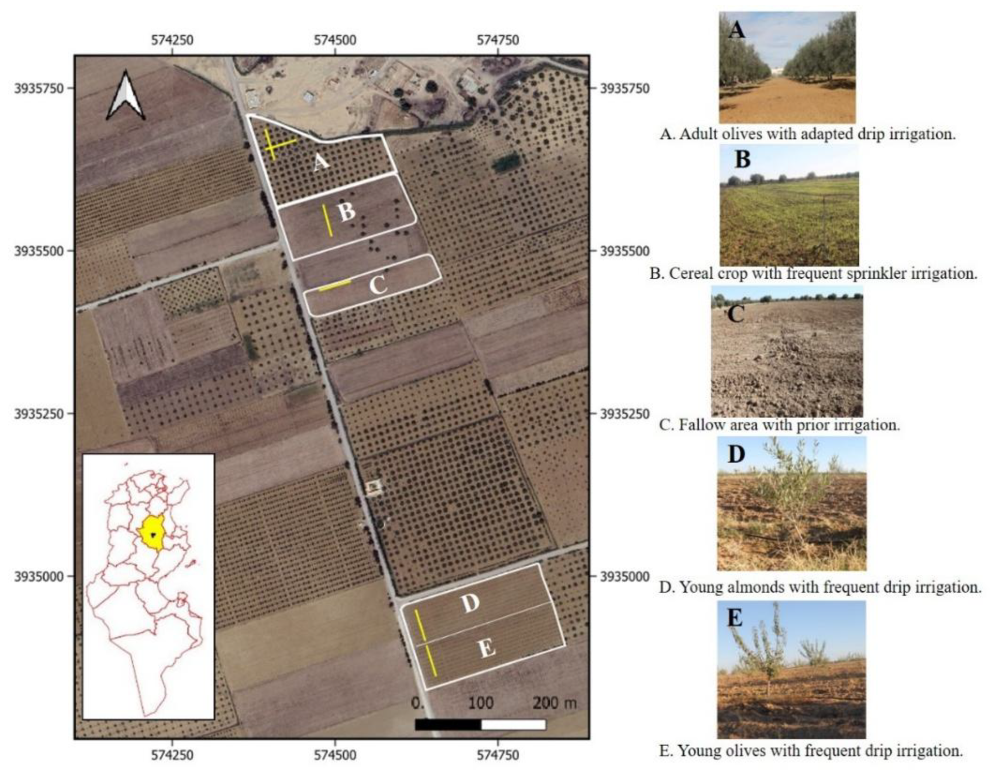
Figure 2.
Each sounding consists in positioning the EM38 and EM31 instruments at different heights from the ground (h = 0 to 95 cm) in both HCP and VCP configurations (right). The 6 geometries allow for sensing at 6 different depths as illustrated by the corresponding 1D sensitivity functions (left), which we computed using the thin layer perturbation approach [36,40].
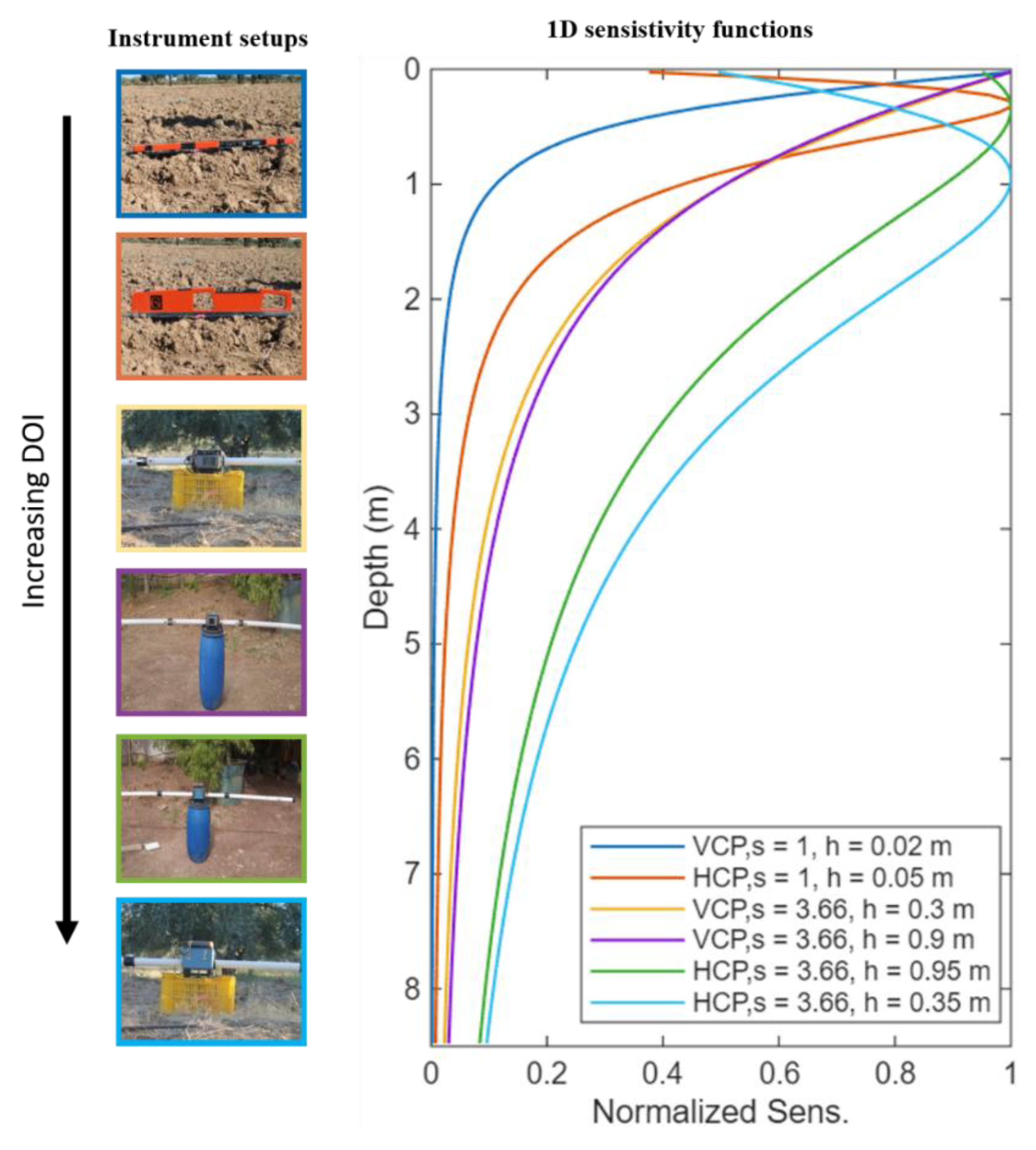
Figure 3.
LIN and robust (full theory) apparent conductivity data for six soundings, each being representative of the six profiles, which are considered in this study. For each sounding, the six channels’ points are shown from top to bottom following increased depths of investigation, which were derived from the analysis of the vertical sensitivity computation (Figure 2).
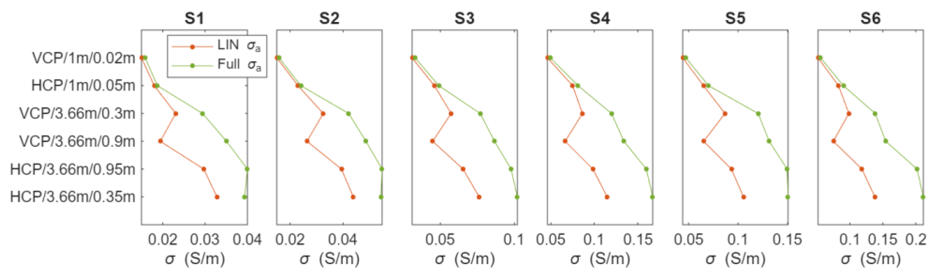
Figure 4.
Principle of the laterally constrained inverse modeling used to interpret the profile of multi-channel FD-EMI ECa data. The 6 channels correspond to the different instrument geometries, which are described in Figure 2. All the profiles contain N_s=51 soundings and were inverted by considering stitched subsurface layered media composed of N_l=20 layers distributed between 0 and 5 m below ground surface.
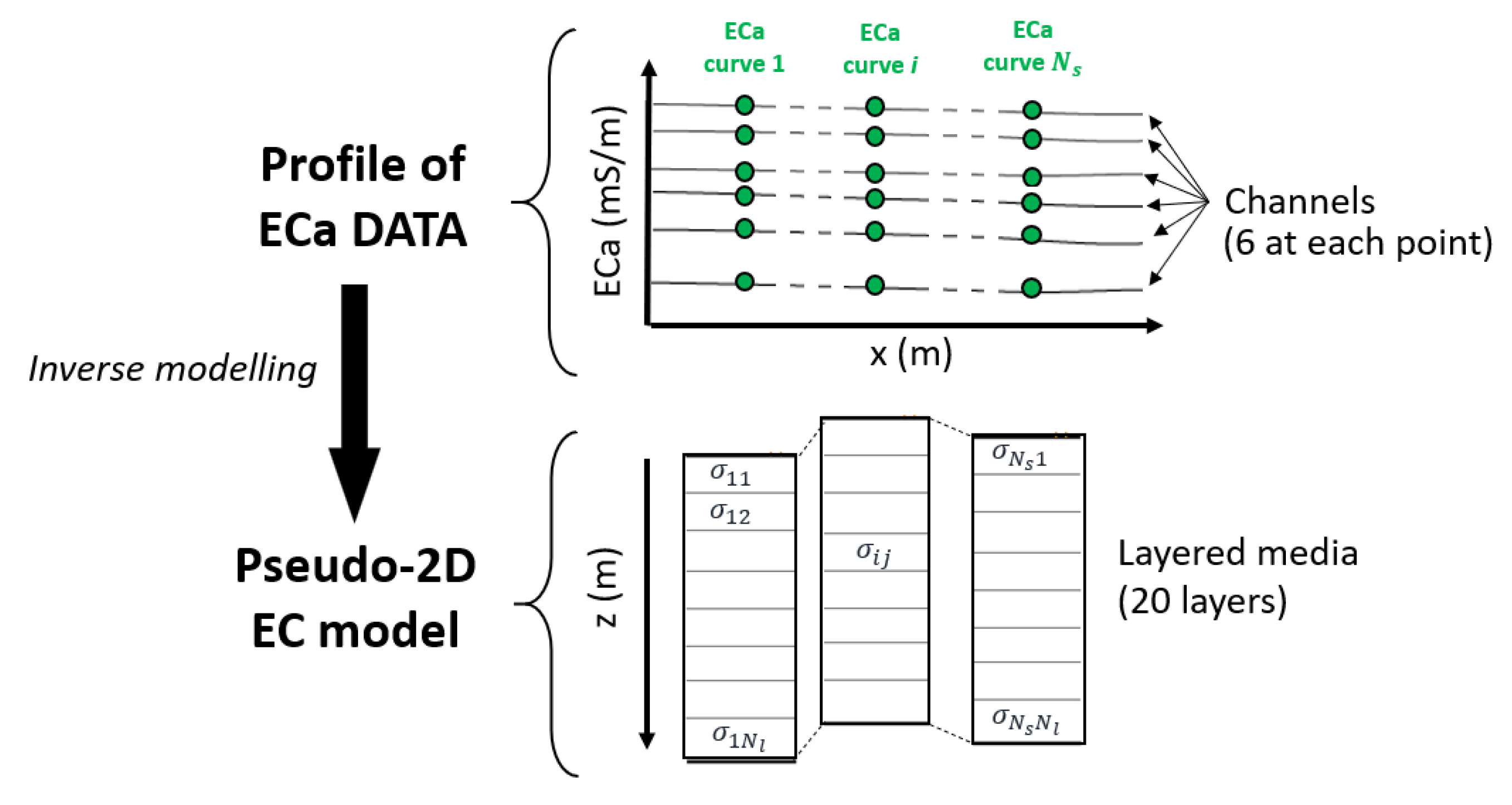
Figure 5.
The distribution of robust ECa data measured along the six different segments and comparison of the average apparent conductivity determined by VCPEM38 Vs VCPEM31 and VCPEM38 Vs VCPEM31 as a function of the segments. Intervals are standard deviations. Abbrev. S1&S2: Adult olives with low frequency adapted irrigation system, S3 (NI): Fallow area non-irrigated, S3 (Res): Fallow area with residual irrigation S4&S5: Young olives and almonds with high frequency drip irrigation, S6: Cereals with high frequency sprinkler irrigation.
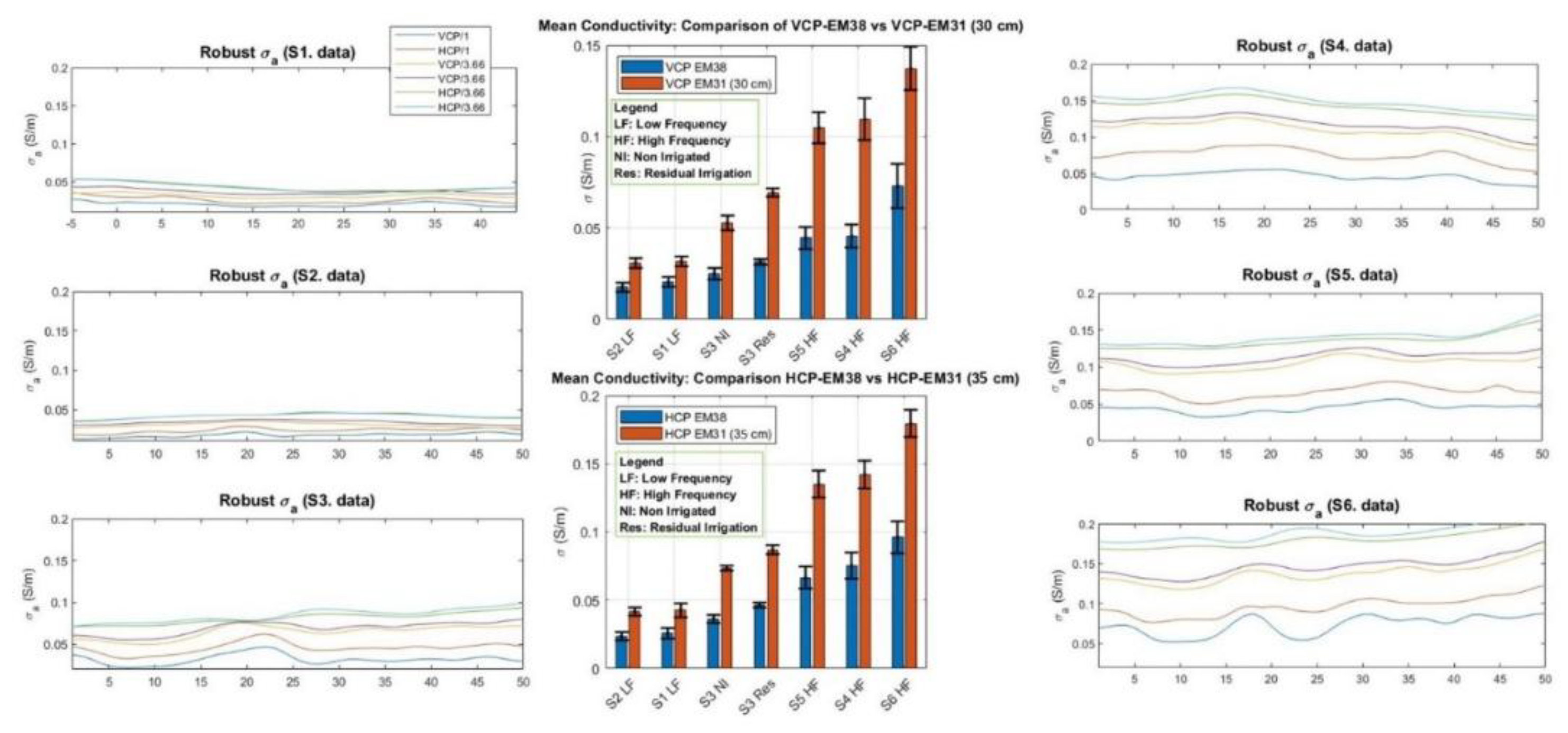
Figure 6.
Distribution of soil salinity according to depth and irrigation regime.
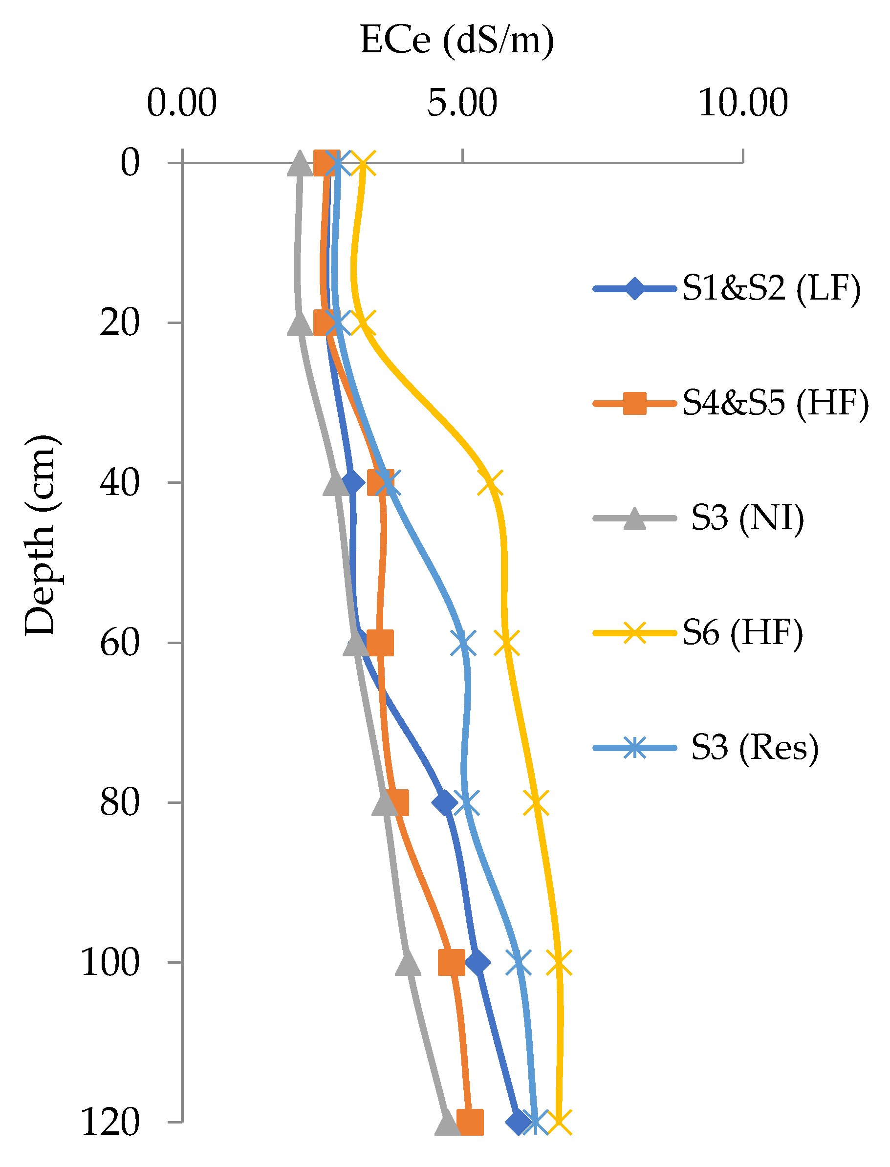
Figure 7.
Pseudo 2-D inversion of apparent conductivity data for the six profiless under different irrigation management regime and their average versus depth (center graphic). Abbrev. S1, S2: Adult olives with low frequency drip irrigation system, S3 Fallow area with residual irrigation, S4, S5: Young olives and almonds with high frequency drip irrigation, S6: Cereals with high frequency sprinkler irrigation.
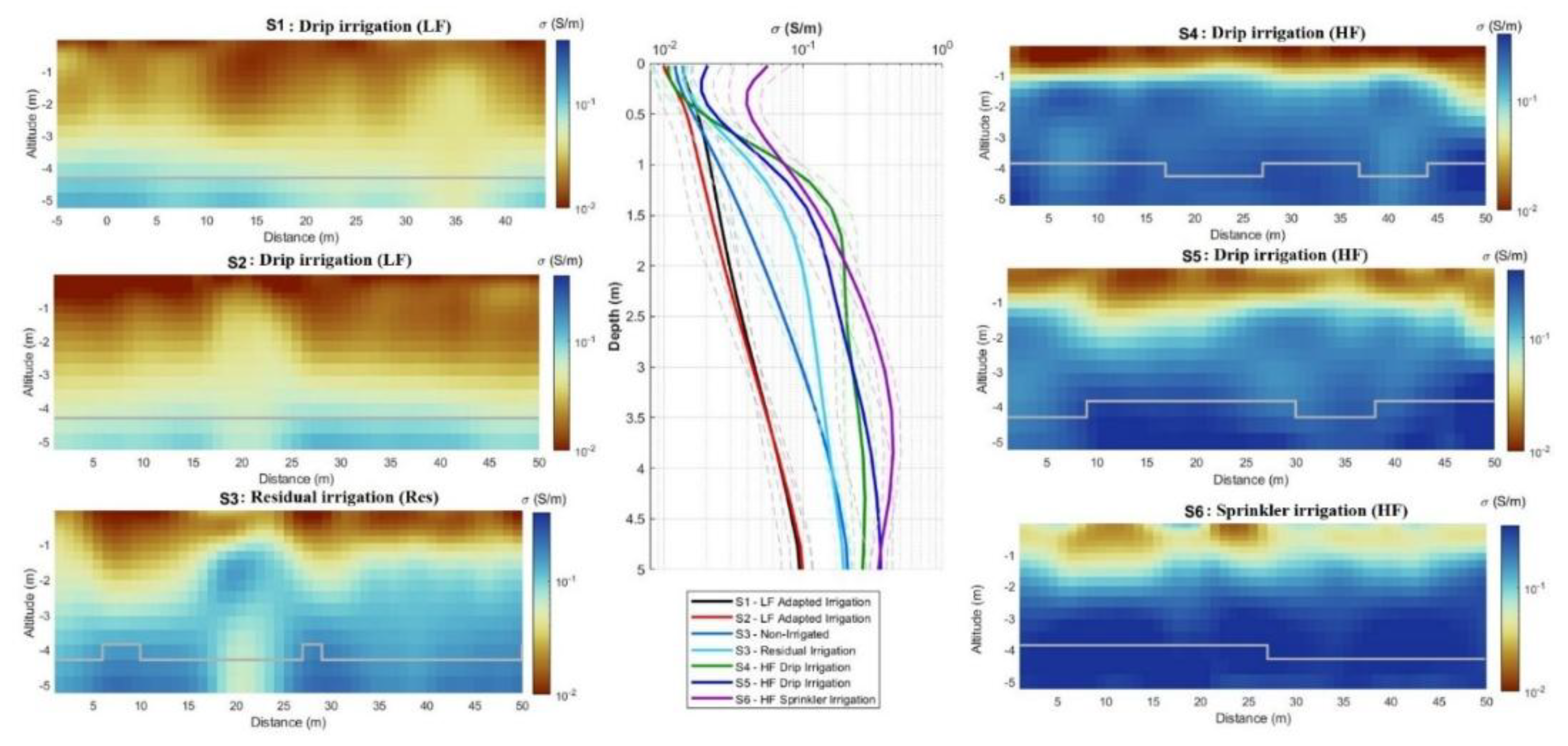
Figure 8.
The inverted ECa data measured along the segments of adult olives S1 and S2 and the effect of trees. Abbrev. S1, S2: Adult olives with low frequency drip irrigation system.
Figure 8.
The inverted ECa data measured along the segments of adult olives S1 and S2 and the effect of trees. Abbrev. S1, S2: Adult olives with low frequency drip irrigation system.
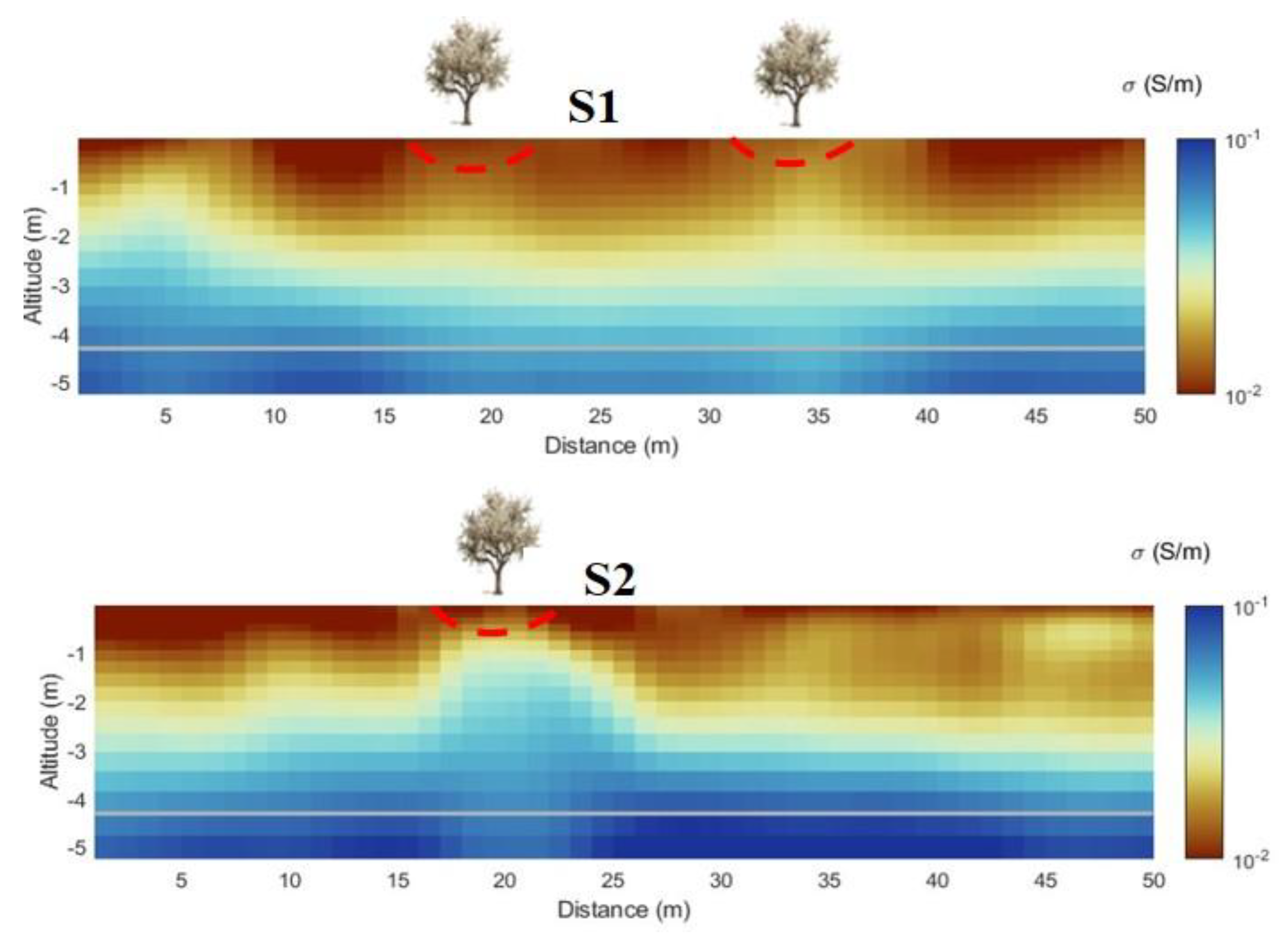
Figure 9.
Mapping of measured ECa in both horizontal and vertical operation modes, at measurement heights of 2 cm, 5 cm, 35 cm, 32 cm, and 35 cm (May 2024), shows an increase in ECa at x = 5 m, x = 20 m, and x = 35 m.
Figure 9.
Mapping of measured ECa in both horizontal and vertical operation modes, at measurement heights of 2 cm, 5 cm, 35 cm, 32 cm, and 35 cm (May 2024), shows an increase in ECa at x = 5 m, x = 20 m, and x = 35 m.
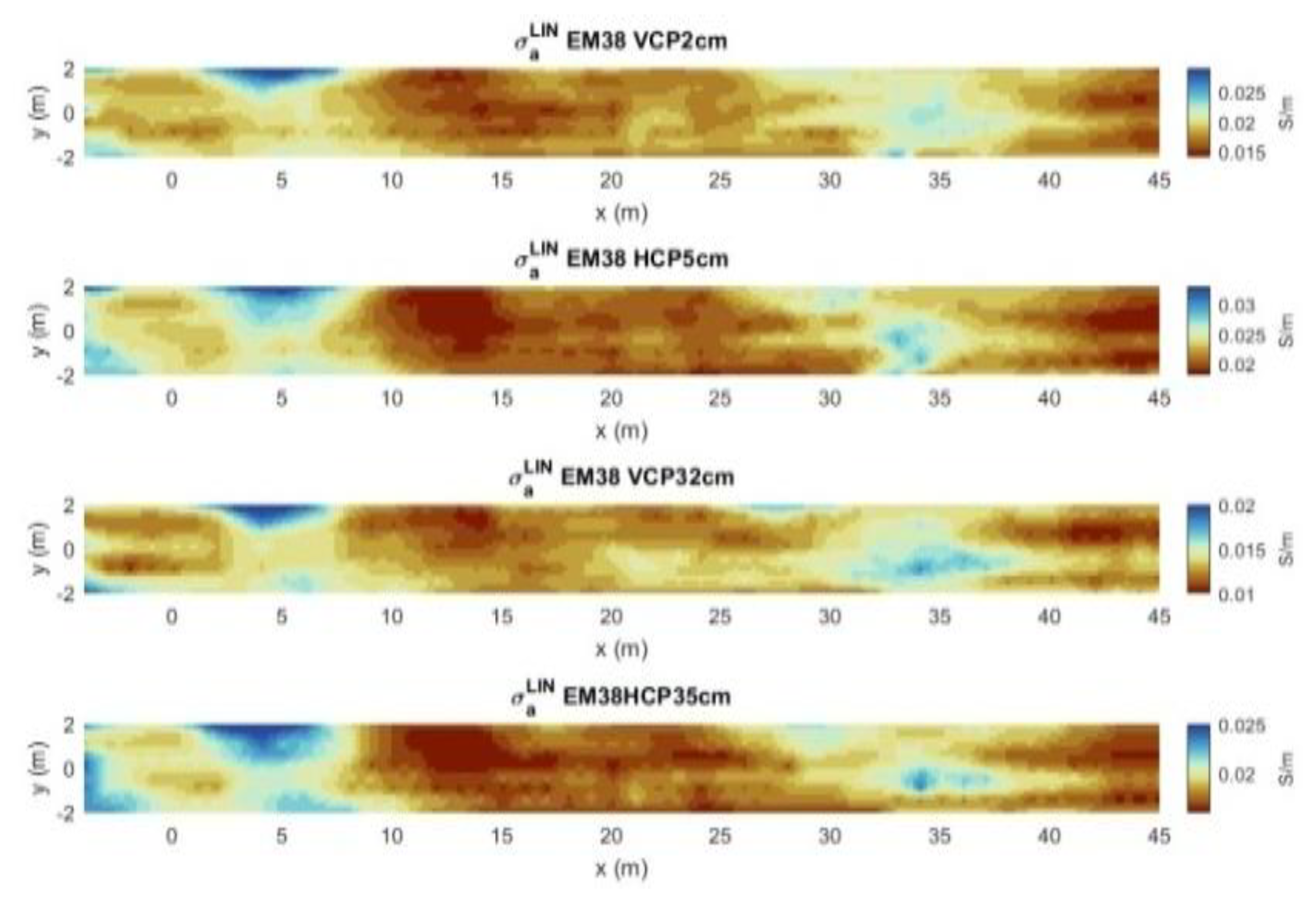
Figure 10.
Inversion results varied between the drip and sprinkler irrigation systems. (a) Segment of young almonds (b) Segment of young olives with high frequency (HF) drip irrigation (c) Segment of cereals with high frequency (HF) sprinkler irrigation (d) Corresponding mean results and their standard deviation for each pseudo-2D model layer.
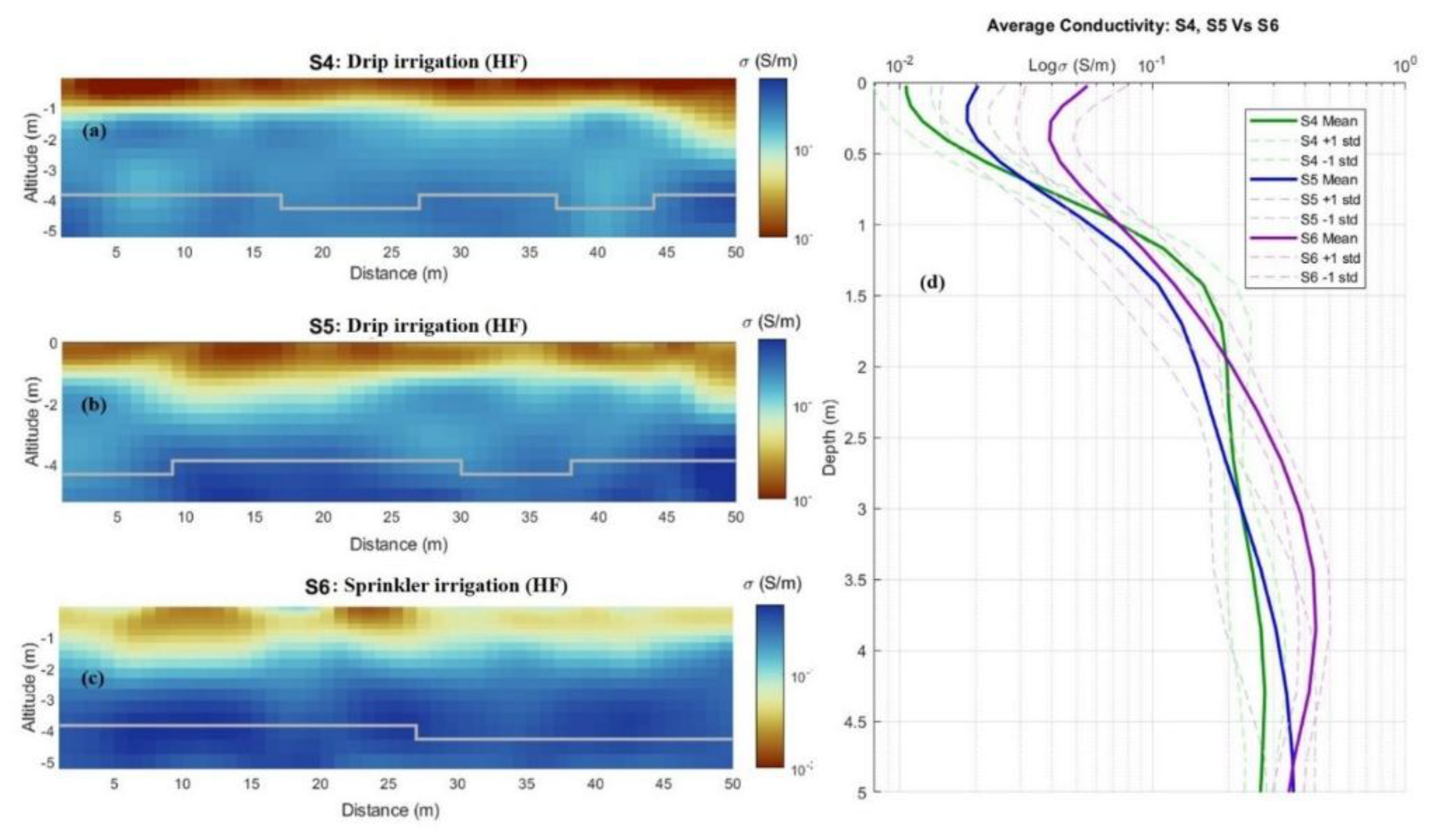
Figure 11.
Inversion results varied depending on the frequency of the drip irrigation system (low or high). (a) First segment of adult olives irrigated with low frequency irrigation (LF). (b) Second segment of adult olives irrigated with low frequency irrigation (LF). (c) Segment young almonds with high frequency irrigation (HF). (d) Segment of olives with high frequency irrigation (HF). (e) Corresponding mean results and their standard deviation for each pseudo-2D model layer.
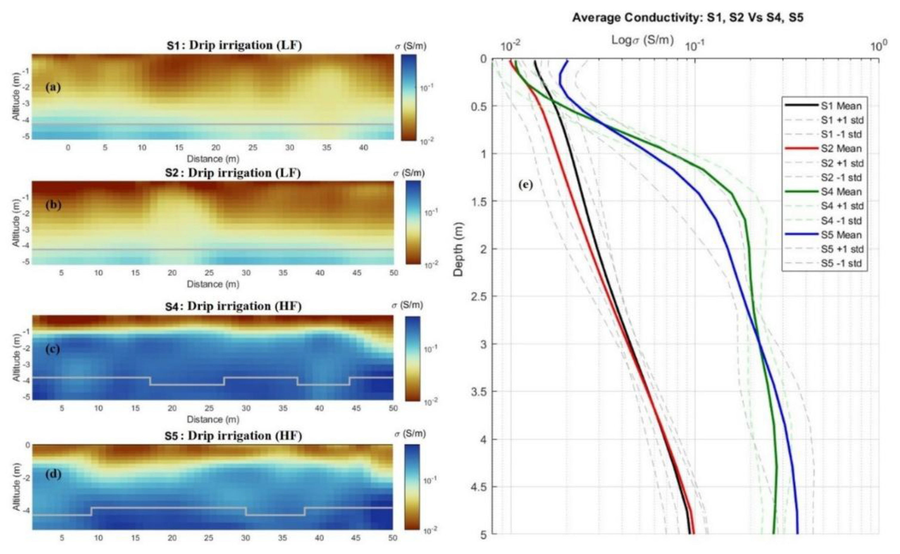
Figure 12.
Inversion results along a fallow area S3 (a) and Corresponding mean results and their standard deviation for each pseudo-2D model layer (b).
Figure 12.
Inversion results along a fallow area S3 (a) and Corresponding mean results and their standard deviation for each pseudo-2D model layer (b).
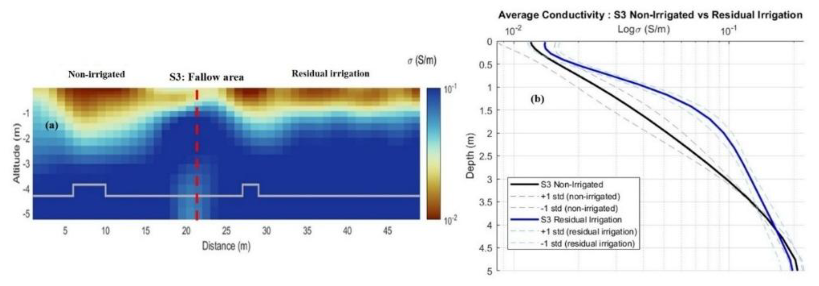
Figure 13.
Inversion results in both periods (a) May 2024 (b) November 2023 and corresponding mean results and their standard deviation for each pseudo-2D model layer (c).
Figure 13.
Inversion results in both periods (a) May 2024 (b) November 2023 and corresponding mean results and their standard deviation for each pseudo-2D model layer (c).
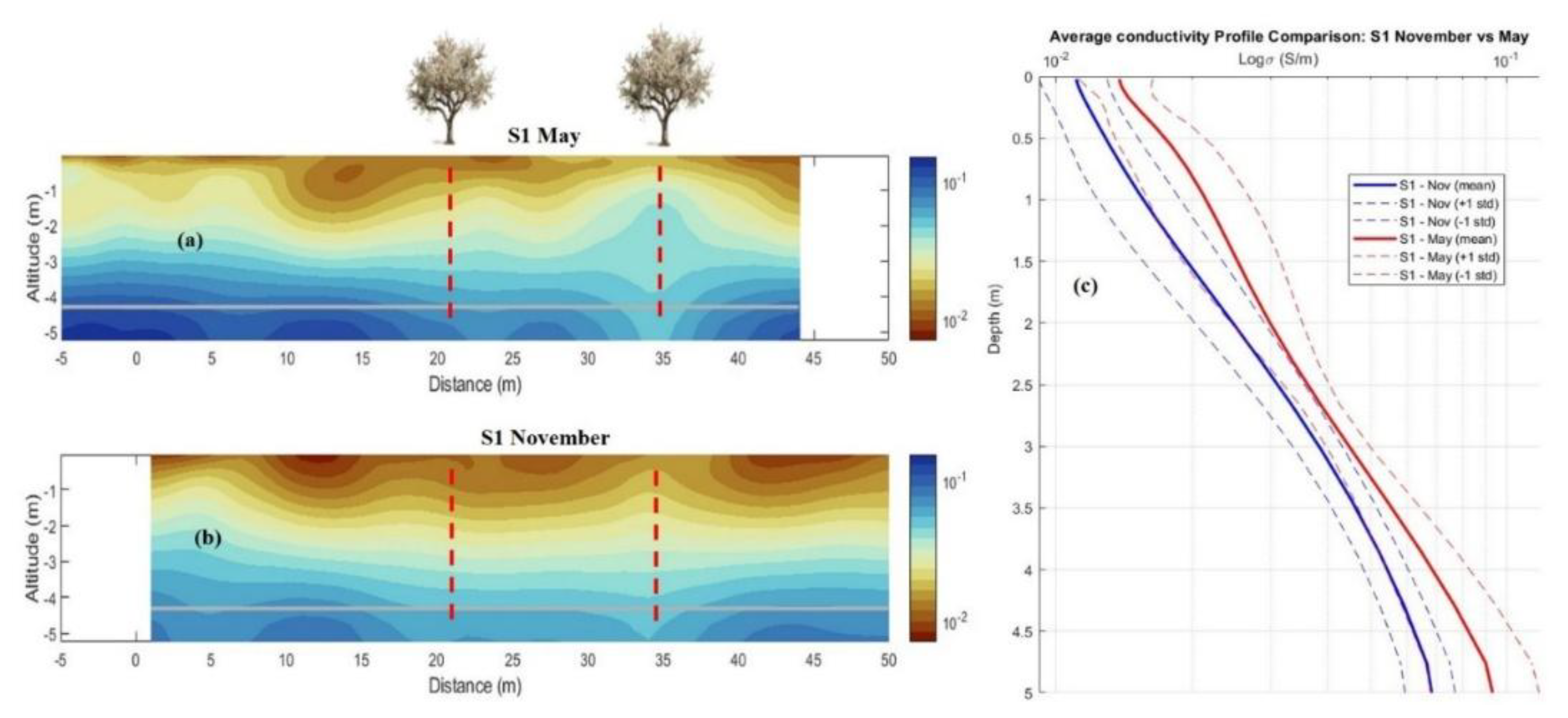

Table 1.
Average moisture content (%) and ECe (dS/m) (N=133).
| Parameters | Moisture content (%) | ECe (dS/m) |
|---|---|---|
| Mean | 11 | 3.99 |
| Median | 10 | 3.75 |
| Min. | 5 | 1.71 |
| Max. | 17 | 8.92 |
| CV (%) | 32 | 38 |
Table 2.
Adopted salinity scale.
| Salinity | ECe | ECa(rounded values) |
|---|---|---|
| Low | <2 | <40 |
| Medium | 2-4 | 40-60 |
| High | >4 | >60 |
Table 3.
Grouping of segments by land use and irrigation system management.
| Segments | Land use | Irrigation system management |
|---|---|---|
| S1 and S2 | Adult trees(Mature olive trees) | Adapted drip irrigation |
| S4 and S5 | Young trees(Young almond and olive trees) | Frequent drip irrigation |
| S6 | Irrigated Cereal (wheat) | Frequent sprinkler irrigation |
| S3 | Fallow land with irrigated antecedent | Irrigation stopped from 2019 |
Disclaimer/Publisher’s Note: The statements, opinions and data contained in all publications are solely those of the individual author(s) and contributor(s) and not of MDPI and/or the editor(s). MDPI and/or the editor(s) disclaim responsibility for any injury to people or property resulting from any ideas, methods, instructions or products referred to in the content. |
© 2025 by the authors. Licensee MDPI, Basel, Switzerland. This article is an open access article distributed under the terms and conditions of the Creative Commons Attribution (CC BY) license (http://creativecommons.org/licenses/by/4.0/).
Copyright: This open access article is published under a Creative Commons CC BY 4.0 license, which permit the free download, distribution, and reuse, provided that the author and preprint are cited in any reuse.


