
Submitted:
12 April 2024
Posted:
12 April 2024
You are already at the latest version
Abstract
In the last decade Electromagnetic Induction (EMI) measurements have been increasingly used for investigating the soil salinization caused by the use of brackish or saline water as irrigation source. EMI measurements proved to be a powerful tool for providing spatial information of the investigated soil because of the strict correlation between the output geophysical parameter, i.e. the electrical conductivity, to soil moisture and salinity. In addition, their non-invasive nature and their capability to collect a high number of data over broad areas and in relatively short time, makes these measurements attractive for monitoring flow and transport dynamics, otherwise undetectable with conventional measurements. In an experimental field, EMI measurements were collected during the growth season of the tomato, irrigated with three different irrigation strategies. The data were collected over three months in a time-lapse mode in order to visualize changes in electrical conductivity to be associated with soil salinity. A rigorous time-lapse inversion procedure has been set for modeling the soil salinization induced by brackish irrigation water.
Keywords:
soil salinization
; apparent electrical conductivity
; electromagnetic induction measurements
; time-lapse inversion
1. Introduction
Soil salinization has become one of the major environmental and socioeconomic issues globally and this is expected to be exacerbated further with projected climatic change. Salinity is one of the main soil threats that reduce soil fertility and affect the crop production. salinity can decrease plant growth and water quality resulting in lower crop yields and degraded stock water supplies. Soil salinization increases when brackish or saline water is often used as irrigation source. In such conditions it’s crucial to develop soil monitoring systems able to capture spatial and temporal dynamics with a high degree of accuracy.
Sensors typically used for agricultural purposes are installed in few sparse points at no more than two-three previously defined depths. In the last decade apparent electrical conductivity, defined as ECa, has been increasingly used for investigating soil properties because it is influenced by a huge range of soil properties, mainly soil moisture and salinity.
Geospatial ECa measurements are reliable and very easy to be collected because they don’t require ground contact and, for this reason, they allow a huge spatial coverage at different depths in limited time. In addition, repeating over time data collection in the same area, i.e. in time-lapse mode, allows for detecting temporal variations of the ECa to be correlated with soil properties that changes during time. Over time this parameter has been widely used as proxy for investigating soil salinity, as recent studies confirm. Corwin et al. [1] improved guidelines broaden the scope of application of ECa-directed soil sampling to map field-scale salinity on orchards under drip irrigation. Vanderlinden et al. [2] highlighted the potential of ECa to perform salinity monitoring at the field or farm scale. Emmanuel et al. [3] validated the potential of extending EMI for characterizing wetland soil properties, such as salinity, improving sampling plans, and interpolating soil property estimates to unsampled regions. Scudiero et al. [4] performed ECa survey to identify locations that can be repeatedly sampled to infer the frequency distribution of soil salinity. Rodrıguez-Perez et al. [5] evaluated the usefulness of apparent electrical conductivity (ECa) data to identify variations in soil chemical and physical properties and moisture content. Lesch et al. [6] documented the spatial salinity mapping using EM survey data. Herrero and Hudnall [7] proved the value of the electromagnetic induction (EMI) to map the salinity of the rootable layer.
When ECa is used for agronomical issues question marks arise. What does ECa means? Is really representative of the soil properties? Can ECa be effectively related to ECe?
ECa is a depth-weighted parameter and gives limited information about the variation of the conductivity with depth. In fact, ECa does not provide a rigorous correlation between earth conductivity structure and measured responses, being affected from several factors such as coil distance and orientation, sensitivity and data error.
In the last few years, an inversion procedure has been implemented in order to produce a reliable soil EC model. The use of inversion codes has grown rapidly as the need for an effective EC distribution in the subsoil has become crucial. Several inversion methods [8,9,10] and software tools ([11,12] have been created for estimating the distribution of soil EC from measured ECa data. These codes solve the complex equations of Maxwell’s electromagnetism to generate forward models used to minimize an objective function and derive models from apparent raw data.
Jadoon et al. [13] identified a quantitative distribution pattern of soil salinity by the joint inversion of multicomponent EMI measurements. Paz et al. [14] highlighted time-lapse EMI as a reliable tool for evaluating the risk of soil salinization and supporting the evaluation and adoption of proper agricultural management strategies. Farzamian et al. [15] inverted ECa data to model the salinity of an oasis in Tunisia which may affect agricultural productivity and the sustainability of crop production. Dakak et al. [16] produced soil salinity maps at various depths through EMI inversion. Shaukat et al. [17] used EMI inversion as a robust and effective method for risk assessment of new shrub plantations. A benefit of the inversion technique lies in its capacity to predict the depth-wise distribution of EC. This facilitates linking laboratory soil samples obtained from different depths at specific sites with the corresponding EC values at those depths. As emphasized by [15], this method permits the incorporation of all soil samples into a single calibration/validation procedure, leading to a more accurate calibration at any chosen depth. Furthermore, employing a larger number of soil samples for calibration and validation enhances the reliability of the outcomes.
In the proposed case study, a time-lapse inversion approach was tested on ECa data collected on an experimental field in the South of Italy where different irrigation strategies have been applied during the growing season of the tomato. The primary objective of time-lapse inversion is to accurately detect variations in conductivity at specific locations across different time intervals. While independent data inversions can be conducted individually, providing insight into changes in modeling results over time through the subtraction of pixel-by-pixel values from a reference dataset, it's important to recognize that temporal changes in conductivity values may not exclusively reflect actual changes in subsurface resistivity depending on data noise level and inversion artifacts. This is particularly true without considering the reference model and prior information [18].
Raw ECa maps, as well as detailed on the experimental set up and soil properties, were already published [19]. In this paper we focused on the inversion of ECa data, both as single snapshot and time-lapse imaging. For the proposed case study, a 2D reference transect was extracted from three different plots subjected to different irrigation strategies (irrigation with freshwater and agro-industrial treated wastewater).
The aim of the paper was: a) to highlight the capability of the inversion tool to produce a detailed 2D EC soil distribution; b) to image the spatio-temporal EC evolution distribution over an irrigation season; c) to assess the impact of brackish water on soil salinization in the short term.
2. Materials and Methods
2.1. Basics of ECa Parameter
ECa is a sensor-based indirect measurement strictly affected to some physical and chemical properties, such as soil salinity, soil moisture, clay content, cation exchange capacity (CEC). Archie [20] and Rhoades et al. [21] developed a theoretical basis for the relationship between ECa and soil properties, such as soil water content, the electrical conductivity of the soil water, soil bulk density, and the electrical conductivity of the soil particles.
According to these premises, over the last decades ECa has been widely used as soil quality indicator [22,23,24].
Over time, several devices have been manufactured both in the time and frequency domain for measuring ECa, according to the Electromagnetic Induction (EMI) theory. An EMI sensor is made of two coils, a transmitter and a receiver. An alternate current is generated by the transmitter coil, spreading into the subsurface and traveling through different materials. According to the electromagnetic induction principles, eddy currents are generated and induce secondary EM fields. A receiver coil records a signal that is the sum of the primary and secondary field.
Figure 1.
Basics of ECa measurements.
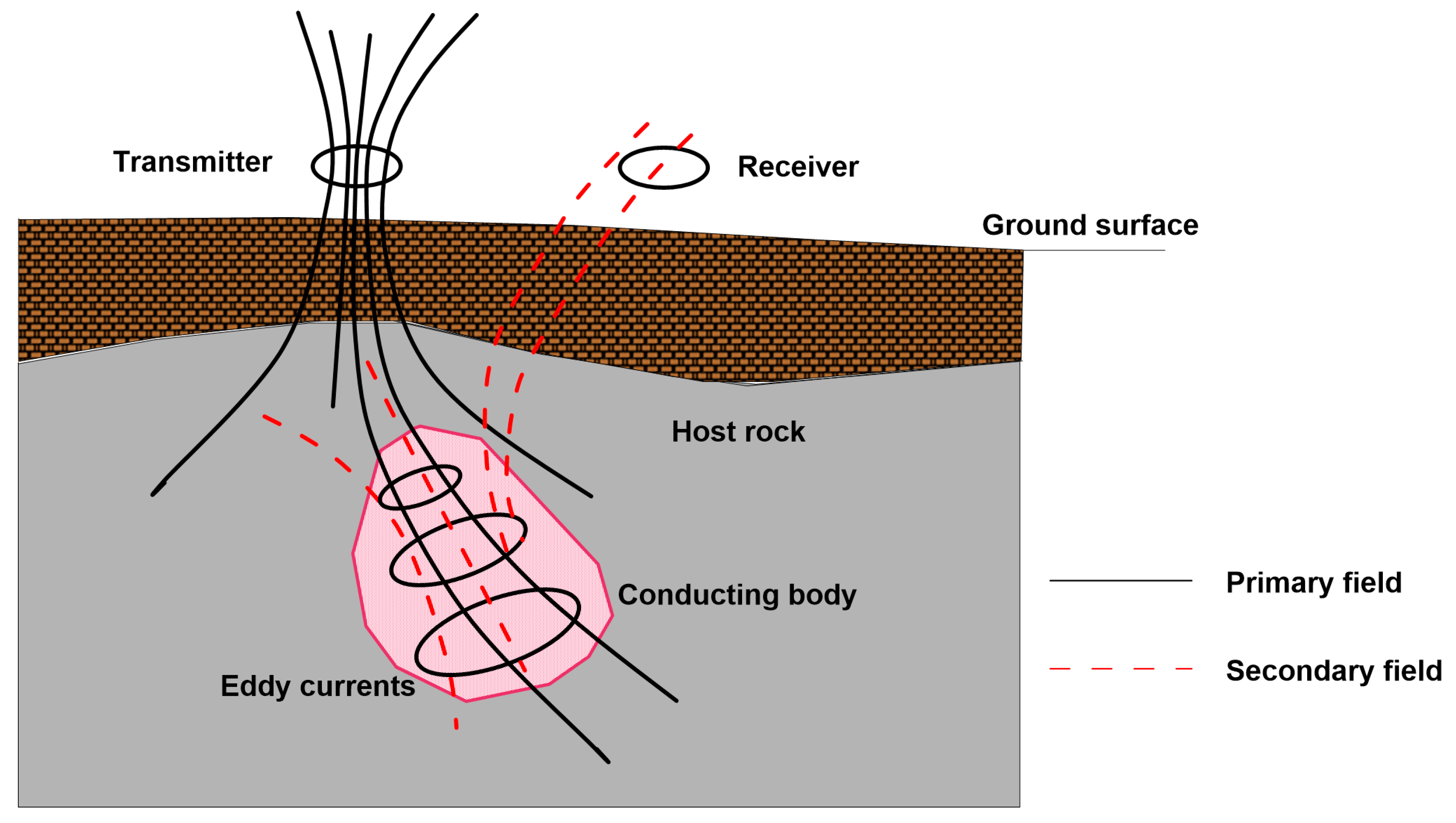
The measured resulting field has an imaginary part of the signal, also called out-of-phase or quadrature (Q) and in-phase (Ph) component. Under simplified conditions, typically defined as Low Induction Number (LIN), the EMI sensors provide directly the subsurface conductivity through Eq.1 [25]:
where f is the frequency (Hz), s is the coil separation (m), μ0 is the magnetic permeability of free space (4π10−7 H/m) and (Hs/Hp) Qu is the Qu component of the secondary Hs to primary Hp magnetic field coupling ratio.
Conversely, the real part, or the in-phase component, of the measured signal is mainly affected by the magnetic permeability of the subsoil.
For the sake of clarity, the ground response depends not only from the soil electrical conductivity but also from instrumental factors such as coil distance, coil orientation and frequency. Particularly, coil distance and orientation affect the depth of penetration of the electromagnetic signal. Placing the coil in vertical position (VCP coil configuration) the top soil layers are investigated, while rotating 90° the coil along the main axis (HCP coil configuration), the signal investigates deeper layers.
Therefore, an ECa value recorded in a point can be defined as an equivalent electrical conductivity of a homogeneous half-space that produces the same measured response to the instrument in a single configuration in that point. This seems quite clear from the analysis of the cumulative sensitivity (CS) function of a measuring device, defined by the ratio between the variation of the output and the variation of the input [26]. The sensitivity function quantifies how much the complex electromagnetic response recorded by the device is affected by a variation in the conductivity and/or permeability of a particular point (area or section) of the subsurface.
Figure 2a,b plots the CS distribution against depth as a function of coil and orientation distances for the CMD-MiniExplorer (GF Instrument s.r.o, Brno), that is the EMI sensor used for collecting field data, made of a cylindrical tube 1.3 m long, with a 30-kHz transmitter coil and three receiver coils with 0.32 m, 0.71 m and 1.18 m offsets, respectively. As clearly observed, the sensitivity changes significantly for three different coil distances and coil orientation.
According to [25], given a specific configuration and under LIN conditions, the effective penetration depth of an EMI sensor corresponds to CS=0.3. Therefore, ECa-derived depths are purely indicative because they depend not only from soil properties but also from instrumental factors.
On the basis of the aforementioned considerations, the assumption that ECa cannot be used to provide quantitative information about the soil properties confirms the need of inverting raw data in order to get a reliable EC distribution in the subsoil.
2.2. Time-Lapse ECa Dataset
The dataset used for time-lapse inversion was collected during the growing season of a tomato crop belonging to a farm located in the South of Italy. The experimental field was randomized with three different irrigation treatments: a) plot A and plot B irrigated with brackish water; b) plot C irrigated with fresh water and conventional fertigation. The EC of the irrigation water is about 2000-2500 µS/cm for plot A and B, 500 µS/cm for plot C.
ECa data were collected in five time points, with the initial measurement taken before the start of the irrigation season (26th June) served as reference time for recording the conductivity changes. Other four datasets were collected with time interval of about 2 weeks (10th July, 24th July, 6th August, 31st August) during the irrigation season. The data were collected in continuous measurement mode by selecting time of measurement equal to 1 s, meaning that the conductivity and in-phase values are measured as average of the values measured during the selected measuring period.
During the last EMI campaign, on 31st August, six soil samples were collected in three points, each belonging to a single plot, at two different depths, 0-0.2 m and 0.2-0.4 m from ground surface in order to provide the ground truth for soil salinity. Details of the sampling procedure and soil analysis are widely described in [19]. In this paper, only the ECe values were extracted in order to provide a correlation function with the inverted EC. In order to test the inversion procedure and compare the findings, nine different 2D EMI transects, corresponding to the locations of soil sampling (see Figure 3) were extrapolated from the three plots.
2.3. Time-Lapse Inversion Procedure
The time-lapse inversion procedure is aimed to estimate the electrical conductivity variations over time along the reference transects. The EM4Soil v4.5 software package [11], based on Occam’s regularization [27], was used to invert the ECa data. The code uses a quasi 2D inversion, by assuming that below each measured location, a 1-dimensional variation of calculated soil conductivity (EC, mS/m) is constrained by variation under neighboring locations [8].
In the time-lapse inversion procedure, the choice of some parameters is crucial for providing accurate inversion models: a) the starting model for solving the inverse problem; b) the inversion algorithm to be used; c) the spatial damping factor (λ) and d) the temporal damping factor (α) [28].
Two inversion algorithms, S1 and S2 [29], provide a different level of constrain to the model parameters. In the S1 algorithm, the corrections to the model parameters at each iteration are calculated by solving the system of equations:
where δp is the vector comprising corrections of the parameters (logarithm of conductivities, pj) of an initial model; b is the vector containing the differences between the logarithm of the observed and calculated apparent conductivities. J is the Jacobian matrix and λ is aforementioned damping factor.
Conversely, the S2 option has one more constrain (Eq.3) and would produce smoother results than S1.
where p0 refers to a reference model.
The spatial smoothing or damping factor λ [30] determines the amplitude of the parameter corrections in the space domain which controls the balance between data fit and model roughness. The selection of λ is determined either through the "L curve" method [31] or through trial and error to determine the value that most accurately represents the expert expectations based on the study site and data fit. A smaller damping factor tends to refine more detailed model parameters, especially in areas with larger expected spatial variability [32]. The temporal damping factor α is a regularization factor that gives the weight for minimizing the temporal changes in the conductivity along the time [28]. As the α value increases, the resulting reference models from the inversion become more similar. A value of zero indicates that no temporal constraints are applied, resembling a traditional independent inversion.
A linear solution, based on the ECa cumulative response (CF) was used for forward calculations in order to convert depth-profile EC to ECa [25]. In our study case, both S1 and S2 algorithms were tested and no substantial differences were observed in the model output. The outputs obtained with S2 algorithm are shown in the section Results. A uniform starting model considering the average ECa value for each plot (EC=100 mS/m for plot A and B, EC=60 mS/m for plot C) was considered for solving the inversion problem, while λ and α parameters were set to 0.07 and 0.05, respectively. These parameter sets were selected after conducting several tests and comparing the results in terms of inversion misfit.
In the pre-processing stage, a single dataset containing all the ECa readings obtained over space and time was defined as input for EM4SOIL code.
3. Results
The inversion was performed for the nine selected EMI transects. As the findings of the inversion results are consistent for the plots subjected to the same irrigation strategies, for simplicity we show a single time-lapse EMI inversion for plot A, B and C.
The inversion results are visualized as static 2D EC images and normalized time-lapse EC differences. For a clear comparison of the soil response to different irrigation strategies, both results are scaled with the same color range.
Figure 4 shows the inverted EC for transect corresponding to plot A, irrigated with brackish water, at five different time points.
At the reference time t1 (26th June) a two layers’ model was identified: a) low conductive top layer (EC<60 mS/m at z < 0.5 m from ground surface); b) high conductive bottom layer (200<EC<60 mS/m). During the irrigation season, the top resistive layer became conductive, while the bottom conductive layer experienced a decrease in conductivity.
Variations in EC over time are clearly observed in Figure 5. After two weeks from the start of irrigation (Figure 5a), slight changes can be observed with the positive changes in yellow area and negative changes in green area. Over time, EC increasing in the top soil layer and decreasing in the bottom layer become more prevalent, as observed in Figure 5b. This trend intensifies in Figure 5c, which corresponds to the EC distribution after 41 days from the start of irrigation, and persists until the end of the irrigation season (Figure 5d,e).
To evaluate the accuracy of the inverted model, the observed vs calculated fit was visualized for each coil configuration at every observation point. (Figure 6). The RMSE between calculated and observed data provides the error model. Generally, the datasets align along the fit line, although some misfit is evident. This trend is not surprising, given the level of accuracy of the ECa data. In fact, the estimated RMSE is 15 mS/m, roughly equivalent to about 16%, when expressed as the ratio between the RMSE in mS/m and the average value of the observations.
Similar trends are recorded in the transect belonging to the plot B. Figure 7 and Figure 8 correspond to the static 2D images and normalized time-lapse EC differences, respectively. Small differences are visualized in the bottom layer, where less marked decreasing are recorded. In addition, the main increase in EC in the top layer occurs in Figure 7d, corresponding to the EC distribution after 66 days, hence later compared to the plot A.
According to the same procedure used for plot A, the RMSE has been estimated through the misfit between observed and calculated data, corresponding roughly to about 16%.
On the other hand, a different soil response is observed in plot C, irrigated with freshwater. Figure 9 and Figure 10 show less marked variations in EC, both positive and negative. Given the poor salinity in the freshwater used for irrigation, the surficial increase is attributed solely to the increase in moisture content into the soil during the irrigation season, while the decreasing in EC observed in the cross section can be attributed to the root water uptake.
The estimated RMSE for plot C is 9 mS/m, corresponding to about 17%.
4. Discussion
The study has been conducted on tomato plant, moderately tolerant to salinity. Nevertheless, different levels of salts in soil or in the irrigation water can induce changes in plant morphology and physiology and address severe consequences on crop yield [33,34,35]. In addition, the trend of accumulating salts during irrigation season may cause negative implications not only on soil health but also on groundwater quality. In fact, excess salts can be leached by winter rainfalls and pushed in the vadose zone until reaching the aquifer, causing an oversalinization of the water resource [36]. With these premises, the implementation of effective tools able to monitor the salinization dynamics into the soil plays a crucial role.
Two weeks after the start of the irrigation, slight changes in EC are observed (Figure 5a-8a-11a). The positive changes identify soil wetting effects caused by the increase in soil moisture. Conversely, decreases in EC observed below the top layer can be correlated to the root water uptake, which causes a negative conductivity changes, as observed in previous works [37,38,39,40].
The changes in EC emphasize the soil-plant-water interaction during the irrigation season, as Figure 5, Figure 8 and Figure 10 highlight. In particular, at the end of the irrigation season, the inversion of the ECa data well distinguished the salt accumulation in the top soil layer in plots irrigated with brackish water (plots A and B) and the root water uptake in the bottom layer of the three plots (Figure 11). The higher EC differences observed in plots A and B compared with the observations in plot C those irrigated with fresh water (plot C) reflect a reduced root water uptake activity due to the high osmotic pressure that inhibits the water flow from the soil to the plant, as observed in [41,42,43,44]. In the context of saline or brackish groundwater management, these evidences should be taken into account in order to balance water requirement and consumption and, hence, to increase water saving and protect the soil. The lower the salt water required, the lower the accumulation of salts, while preserving the crop yield.
For the sake of clarity, a certain level of noise has been recorded in the raw and inverted data. This is a critical aspect about the processing of ECa data. ECa maps produce a rapid and fast visualization of the soil properties but, at the same time, they don’t provide information about systematic or random errors, above all when the ECa data are collected in the most commonly “continuous mode” of measurement, i.e. when the instrument moves in the field and the displayed ECa value is the average value measured during the set measuring period. Conversely, inverting data allows to estimate a model error, remove data or noisy channels and invert again the filtered datasets.
In addition, the use of ECa data could lead to misleading when a calibration function EC vs ECe is required for converting geophysical data into hydrological properties. In fact, as ECa is a depth-weighted parameter, their practical application could lead to incorrect estimations, due to the different resolution, depth of investigation and sensitivity. Moreover, when data are collected both with HCP and VCP coil configurations, at least two depth-specific calibration functions should be developed, considering that the upper soil layer (0-0.50m) is potentially investigated with three ECa measurements (VCP0.32m, VCP0.71m and HCP0.32m).
On the other hand, using the inverted EC data allows for plotting a single EC vs ECe calibration function because the inverted model provides an estimation of EC distribution at different depths. This is essential when a limited number of soil samples are available as “ground truth” because all inverted EC data can be used in a single calibration function, as the proposed case study.
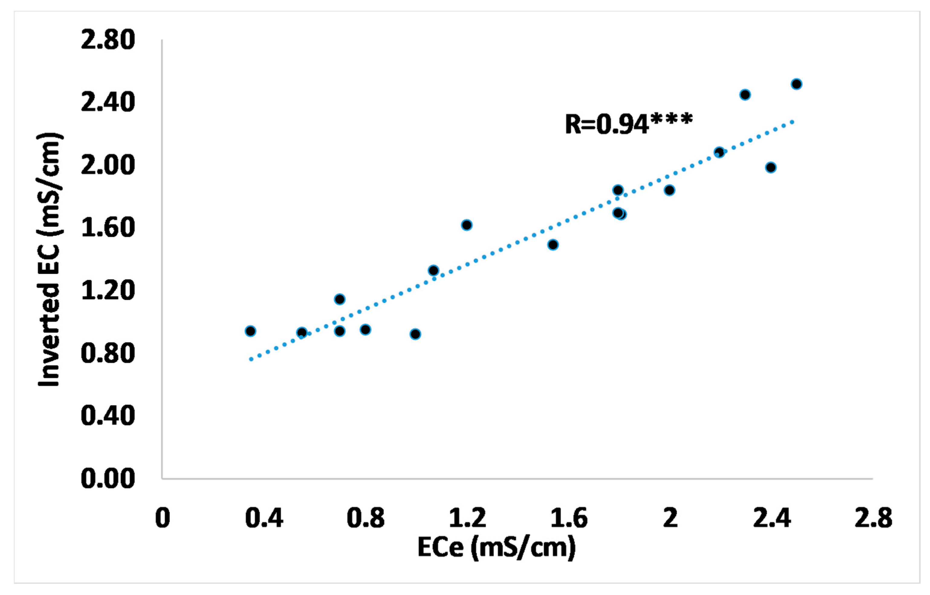
Figure 12 shows the calibration function inverted EC vs ECe, whose values are derived from [19]. For plotting this graph, we have extracted the inverted EMI values for all nine EMI transects. Only one ECe point was removed from the dataset due to an unexplained huge drift from the general trend, probably for an error in soil sampling analysis.
The trend is clear, confirming the assumption that the inversion process improves the soil modeling.
5. Conclusions
In this study, EMI has proven to be an appropriate approach for providing essential information on the soil properties.
This study made use of ECa data collected in time-lapse mode to assess the impact of brackish water used as irrigation source during the tomato growth season. In three plots where different irrigation strategies were used, repeated ECa data were collected at five time points. This approach provided promising answers to the research questions highlighted in the aims of the study. The findings have highlighted how inverted EC allowed to accurately identify soil properties when different irrigation strategies are used.
In fact, a clear soil response to different irrigation water, brackish and freshwater, was observed.
Compared with the traditional raw ECa visualization, the processing of the data through time-lapse inversion allowed for visualizing a higher level of detail of the soil properties. Although this study was conducted in the short term of a single irrigation season, a significant increase in EC in the upper layer could have strong implications in terms of accumulation of salt. At the same time, the activity of water uptake from the roots was imaged, confirming the versatility of the geophysical tool in the agronomic investigation. The inversion of the ECa allowed for defining a single correlation function EC vs ECe, although based on few points, by merging all the data collected at different depths. Depending on the extension of the area to be investigated, a significant number of data points can strengthen the calibration function in order to accurately convert the geophysical outcome into hydrological properties of interest.
The capability of producing an accurate correlation function through the inverted model represents an added value respect to the use of the ECa, that is a depth-weighted parameter and could address meaningless correlations with point scale measurements.
As the electromagnetic data are increasingly widespread in the scientific landscape, it is strongly recommended that the inversion procedure can be routinely used in the comprehension of the soil properties and dynamics.
Author Contributions
Conceptualization, L.D.C and M.F.; methodology, L.D.C. and M.F.; validation, M.F.; formal analysis, L.D.C.; investigation, L.D.C.; resources, L.D.C.; data curation, L.D.C.; writing—original draft preparation, L.D.C.; writing—review and editing, M.F.; visualization, M.F.; supervision, L.D.C. and M.F.; All authors have read and agreed to the published version of the manuscript.
Funding
This research was co-funded by the Regione Puglia as the project “Sistema innovativo di monitoraggio e trattamento delle acque reflue per il miglioramento della compatibilità ambientale ai fini di un’agricoltura sostenibile” – SMARTWATER (No. 5ABY6PO) through the INNONETWORK CALL 2017.
Data Availability Statement
Dataset available on request from the authors.
Acknowledgments
The authors wish to thank Fiordelisi Farm for making the experimental plot facility available to carry out the field experimental activities. A special mention to Giovanni Berardi for his support in field activities and Domenico Bellifemine for his contribution in the technical aspects.
Conflicts of Interest
The authors declare no conflicts of interest.
References
- Corwin, D.L.; Scudiero, E.; Zaccaria, D. Modified ECa – ECe protocols for mapping soil salinity under micro-irrigation. Agric Water Manag, 2022; 269, 107640. [Google Scholar] [CrossRef]
- Vanderlinden, K.; Martínez, G.; Ramos, M.; Laguna, A.; Vanwalleghem, T.; Peña, A.; Carbonell, R.; Ordóñez, R.; Giráldez, J.V. Soil Salinity Patterns in an Olive Grove Irrigated with Reclaimed Table Olive Processing Wastewater. Water 2022, 14, 3049. [Google Scholar] [CrossRef]
- Emmanuel, E.D.; Lenhart, C.F.; Weintraub, M.N.; Doro, K.O. Estimating Soil Properties Distribution at a Restored Wetland Using Electromagnetic Imaging and Limited Soil Core Samples. Wetlands 2023, 43, 39. [Google Scholar] [CrossRef]
- Scudiero, E.; Skaggs, T.H.; Corwin, D.L. Simplifying field-scale assessment of spatiotemporal changes of soil salinity. Sci Total Environ 2017, 587–588, 273–281. [Google Scholar] [CrossRef]
- Rodríguez-Pérez, J.R.; Plant, R.E.; Lambert, J.J.; Smart D., R. Using apparent soil electrical conductivity (ECa) to characterize vineyard soils of high clay content. Precision Agric 2011, 12, 775–794. [Google Scholar] [CrossRef]
- Lesch, S.M.; Corwin, D.L.; Robinson, D.A. Apparent soil electrical conductivity mapping as an agricultural management tool in arid zone soils. Comput Electron Agric 2005, 46, 351–378. [Google Scholar] [CrossRef]
- Herrero, J.; Hudnall, W.H. Measurement of soil salinity using electromagnetic induction in a paddy with a densic pan and shallow water table. Paddy Water Environ 2014, 2014 12, 263–274. [Google Scholar] [CrossRef]
- Monteiro Santos, F.A. 1D laterally constrained inversion of EM34 profiling data. J Appl Geophys 2004, 56, 123–134. [Google Scholar] [CrossRef]
- Moghadas, D. Probabilistic Inversion of Multiconfiguration Electromagnetic Induction Data Using Dimensionality Reduction Technique: A Numerical Study. Vadose Zone J 2019, 18, 180183. [Google Scholar] [CrossRef]
- Narciso, J.; Bobe, C.; Azevedo, L.; Van De Vijver, E. A Comparison between Kalman Ensemble Generator and Geostatistical Frequency-Domain Electromagnetic Inversion: The Impacts on near-Surface Characterization. Geophys 2022, 87, E335–E346. [Google Scholar] [CrossRef]
- Triantafilis, J.; Terhune IV, C.H.; Monteiro Santos, F.A. An inversion approach to generate electromagnetic conductivity images from signal data. Environ Model Softw 2013, 43, 88–95. [Google Scholar] [CrossRef]
- McLachlan, P.; Blanchy, G.; Binley, A. EMagPy: Open-source standalone software for processing, forward modeling and inversion of electromagnetic induction data. Comput and Geosci 2021, 146, 104561. [Google Scholar] [CrossRef]
- Jadoon, K.Z.; Moghadas, D. , Jadoon, A., Missimer, T. M.; Al-Mashharawi, S. K.; McCabe, M. F. Estimation of soil salinity in a drip irrigation system by using joint inversion of multicoil electromagnetic induction measurements. Water Resour Res 2015, 51, 3490–3504. [Google Scholar] [CrossRef]
- Paz, M.C.; Farzamian, M.; Paz, A.M.; Castanheira, N.L.; Gonçalves, M.C. , Monteiro Santos, F. Assessing soil salinity dynamics using time-lapse electromagnetic conductivity imaging. Soil, 2020, 6, 499–511. [Google Scholar] [CrossRef]
- Farzamian, M.; Bouksila, F.; Paz, A.M.; Monteiro Santos, F.; Zemni, N.; Slama, F. Slimane, A.B.; Selim, T.; Triantafilis, J. Landscape-scale mapping of soil salinity with multi-height electromagnetic induction and quasi-3d inversion in Saharan Oasis, Tunisia. Agric Water Manag 2023, 284, 108330. [Google Scholar] [CrossRef]
- Dakak, H.; Huang, J.; Zouahri, A.; Douaik, A.; Triantafilis, J. Mapping soil salinity in 3-dimensions using an EM38 and EM4Soil inversion modelling at the reconnaissance scale in central Morocco. Soil Use Manag 2017, 33, 553–567. [Google Scholar] [CrossRef]
- Shaukat, H.; Flower, K.C.; Leopold, M. Soil Mapping Using Electromagnetic Induction to Assess the Suitability of Land for Growing Leptospermum nitens in Western Australia. Front Environ Sci 2022, 10, 883533. [Google Scholar] [CrossRef]
- Deiana, R.; Cassiani, G.; Kemna, A.; Villa, A.; Bruno, V.; Bagliani, A. An experiment of non-invasive characterization of the vadose zone via water injection and cross-hole time lapse geophysical monitoring. Near Surf Geophys 2007, 2007 5, 183–194. [Google Scholar] [CrossRef]
- De Carlo, L.; Vivaldi, G.A.; Caputo, M.C. Electromagnetic Induction Measurements for Investigating Soil Salinization Caused by Saline Reclaimed Water. Atmosphere 2022, 13, 73. [Google Scholar] [CrossRef]
- Archie, G.E. The Electrical Resistivity Log as an Aid in Determining Some Reservoir Characteristics. Trans Am Inst Min 1942, 146, 54–62. [Google Scholar] [CrossRef]
- Rhoades, J.D.; Manteghi, N.A.; Shrouse, P.J.; Alves, W.J. Soil electrical conductivity and soil salinity: new formulations and calibrations. Soil Sci Soc Am 1989, 53, 433–439. [Google Scholar] [CrossRef]
- Corwin, D.L.; Lesch, S.M.; Oster, J.D.; Kaffka, S.R. Monitoring management-induced spatio–temporal changes in soil quality through soil sampling directed by apparent electrical conductivity. Geoderma, 2006, 131, 369–387. [Google Scholar] [CrossRef]
- Triantafilis, J.; Lesch, S.M. Mapping clay content variation using electromagnetic techniques. Comp Electron Agric 2005, 46, 203. [Google Scholar] [CrossRef]
- Atwell, M.A.; Wuddivira, M.N. Electromagnetic-induction and spatial analysis for assessing variability in soil properties as a function of land use in tropical savanna ecosystems. SN Appl Sci 2019, 1, 856. [Google Scholar] [CrossRef]
- McNeill, J. D. Electromagnetic terrain conductivity measurement at low induction numbers. Mississauga, Canada. 1980. Geonics Limited. http://www.geonics.com/pdfs/technicalnotes/tn6. (accessed on 1 November 2017).
- Deidda, G.P.; Díaz de Alba, P.; Pes, F.; Rodriguez, G. Forward Electromagnetic Induction Modelling in a Multilayered Half-Space: An Open-Source Software Tool. Remote Sens 2023, 15, 1772. [Google Scholar] [CrossRef]
- Sasaki, Y. Two-dimensional joint-inversion of magnetotelluric and dipole–dipole resistivity data. Geophysics 1989, 54, 254–262. [Google Scholar] [CrossRef]
- Farzamian, M.; Autovino, D.; Basile, A.; De Mascellis, R.; Dragonetti, G.; Monteiro Santos, F.; Binley, A.; Coppola, A. Assessing the dynamics of soil salinity with time-lapse inversion of electromagnetic data guided by hydrological modelling. Hydrol Earth Syst Sci, 2021, 25, 1509–1527. [Google Scholar] [CrossRef]
- Sasaki, Y. Full 3-D inversion of electromagnetic data on PC. J Appl Geophys 2001, 46, 45–54. [Google Scholar] [CrossRef]
- Triantafilis, J.; Monteiro Santos, F.A. Electromagnetic conductivity imaging (EMCI) of soil using a DUALEM-421 and inversion modelling software (EM4Soil). Geoderma 2013, 211-212, 28–38. [Google Scholar] [CrossRef]
- Hansen, P.C. Rank-Deficient and Discrete Ill-Posed Problems: Numerical Aspects of Linear Inversion; Society for Industrial and Applied Mathematics (SIAM): Philadelphia, PA, USA, 1998. [Google Scholar] [CrossRef]
- Farzamian, M.; Ribeiro, J.A.; Khalil, M.A.; Monteiro Santos, F.A.; Kashkouli, M.F.; Bortolozo, C. A.; Mendonça, J. L. Application of Transient Electromagnetic and Audio-Magnetotelluric Methods for Imaging the Monte Real Aquifer in Portugal. Pure Appl Geophys 2019, 176, 719–735. [Google Scholar] [CrossRef]
- Roșca, M.; Mihalache, G.; Stoleru, V. Tomato responses to salinity stress: From morphological traits to genetic changes. Front Plant Sci 2023, 14, 1118383. [Google Scholar] [CrossRef]
- Al-Daej, M.I. Salt tolerance of some tomato (Solanum lycoversicum L.) cultivars for salinity under controlled conditions. Am J Plant Physiol 2018, 13, 58–64. [Google Scholar] [CrossRef]
- Zaki, H.E.M.; Yokoi, S. A comparative in vitro study of salt tolerance in cultivated tomato and related wild species. Plant Biotechnol 2016, 33, 361–372. [Google Scholar] [CrossRef] [PubMed]
- Greene, R.; Timms, W.; Rengasamy, P.; Arshad, M.; Cresswell, R. Soil and Aquifer Salinization: Toward an Integrated Approach for Salinity Management of Groundwater. In: Integrated Groundwater Management. Jakeman, A.J., Barreteau, O., Hunt, R.J., Rinaudo, JD., Ross, A. Eds.; Publisher: Springer, Cham, Switzerland, 2016; pp.377-412. [CrossRef]
- Srayeddin, I.; Doussan, C. Estimation of the spatial variability of root water uptake of maize and sorghum at the field scale by electrical resistivity tomography. Plant Soil 2009, 319, 185–207. [Google Scholar] [CrossRef]
- Ursino, N.; Cassiani, G.; Deiana, R.; Vignoli, G.; Boaga, J. Measuring and modelling water related soil–vegetation feedbacks in a fallow plot. Hydrol Earth Syst Sci 2013, 18, 1105–1118. [Google Scholar] [CrossRef]
- Cassiani, G.; Boaga, J.; Rossi, M.; Putti, M.; Fadda, G.; Majone, B.; Bellin, A. Soil–plant interaction monitoring: small scale example of an apple orchard in Trentino, North-Eastern Italy. Sci Total Environ 2016, 543, 851–861. [Google Scholar] [CrossRef]
- De Carlo, L.; Battilani, A.; Solimando, D.; Caputo, M.C. Application of time-lapse ERT to determine the impact of using brackish wastewater for maize irrigation. J Hydrol 2019, 582, 124465. [Google Scholar] [CrossRef]
- Wang, L.; Ning, S.; Chen, X.; Li, Y.; Guo, W.; Ben-Gal, A. Modeling tomato root water uptake influenced by soil salinity under drip irrigation with an inverse method. Agric Water Manag 2021, 255, 106975. [Google Scholar] [CrossRef]
- Chaali, N.; Comegna, A.; Dragonetti, G.; Todorovic, M.; Albrizio, R.; Hijazeen, D.; Lamaddalena, N.; Coppola, A. Monitoring and Modeling Root-uptake Salinity Reduction Factors of a Tomato Crop under Non-uniform Soil Salinity Distribution. Procedia Environ. Sci. 2013, 19, 643–653. [Google Scholar] [CrossRef]
- Steudle, E. Water uptake by plant roots: an integration of views. Plant and Soil 2000, 226, 45–56. [Google Scholar] [CrossRef]
- Lu, Y.; Fricke, W. Salt Stress—Regulation of Root Water Uptake in a Whole-Plant and Diurnal Context. Int J Mol Sci 2023, 24, 8070. [Google Scholar] [CrossRef]
Figure 2.
Normalized cumulative sensitivity (CS) for the three Mini-Explorer sensors S1, S2 and S3: a) VCP configuration and b) HCP coil configuration.
Figure 2.
Normalized cumulative sensitivity (CS) for the three Mini-Explorer sensors S1, S2 and S3: a) VCP configuration and b) HCP coil configuration.
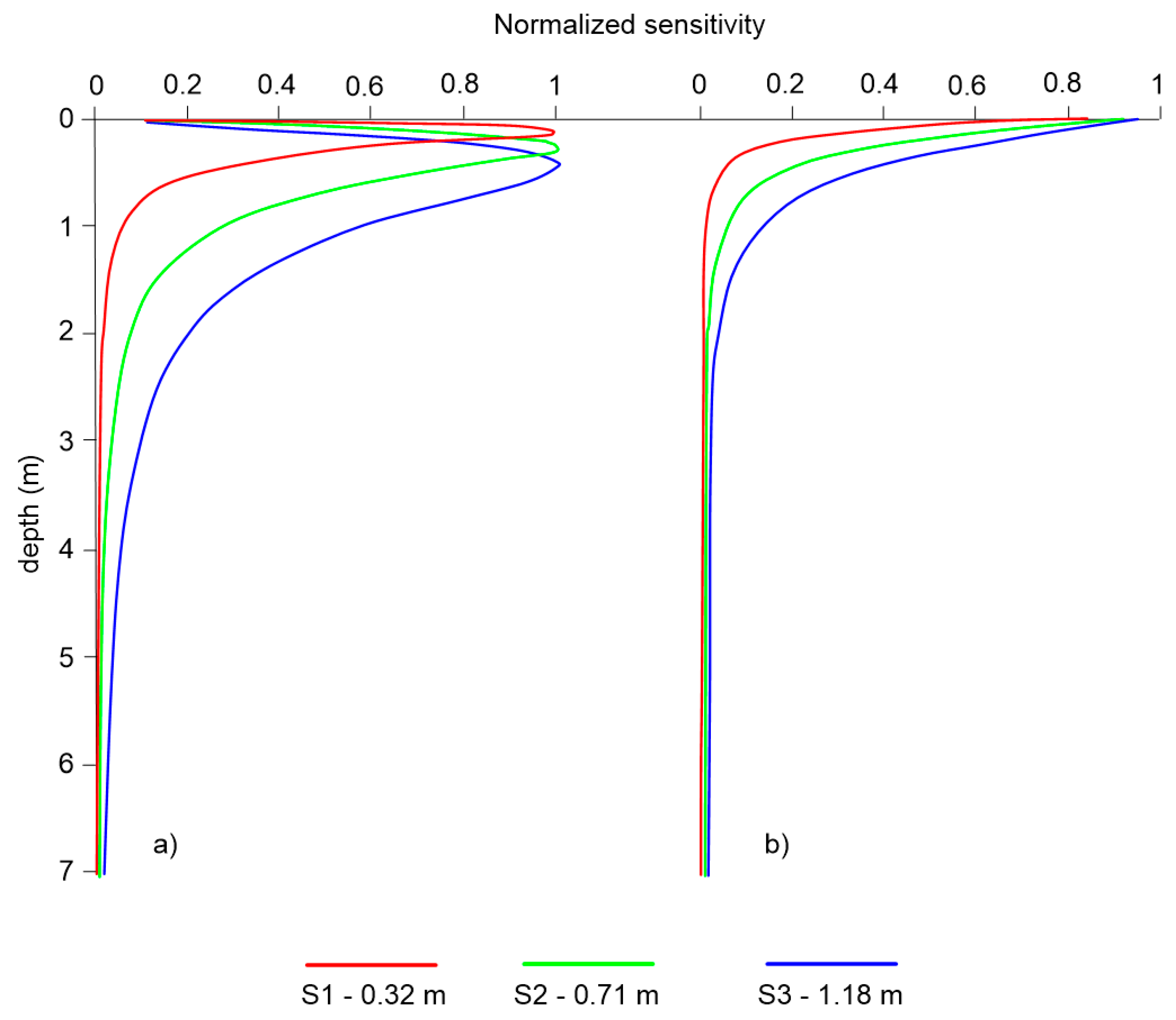
Figure 3.
Distribution of ECa data collected in the experimental field.
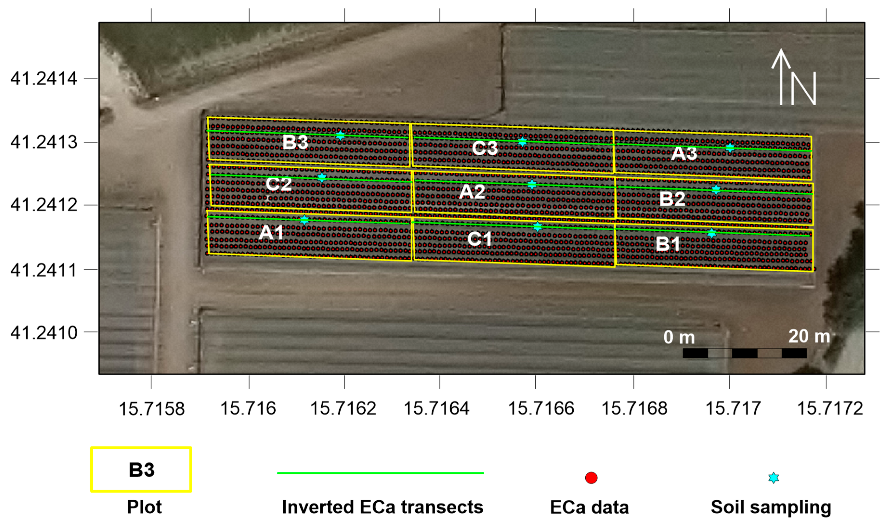
Figure 4.
Inverted EC for transect corresponding to plot A at five different time points: a) 26th June; b) 10th July; c) 24th July; d) 6th August; e) 31st August.
Figure 4.
Inverted EC for transect corresponding to plot A at five different time points: a) 26th June; b) 10th July; c) 24th July; d) 6th August; e) 31st August.
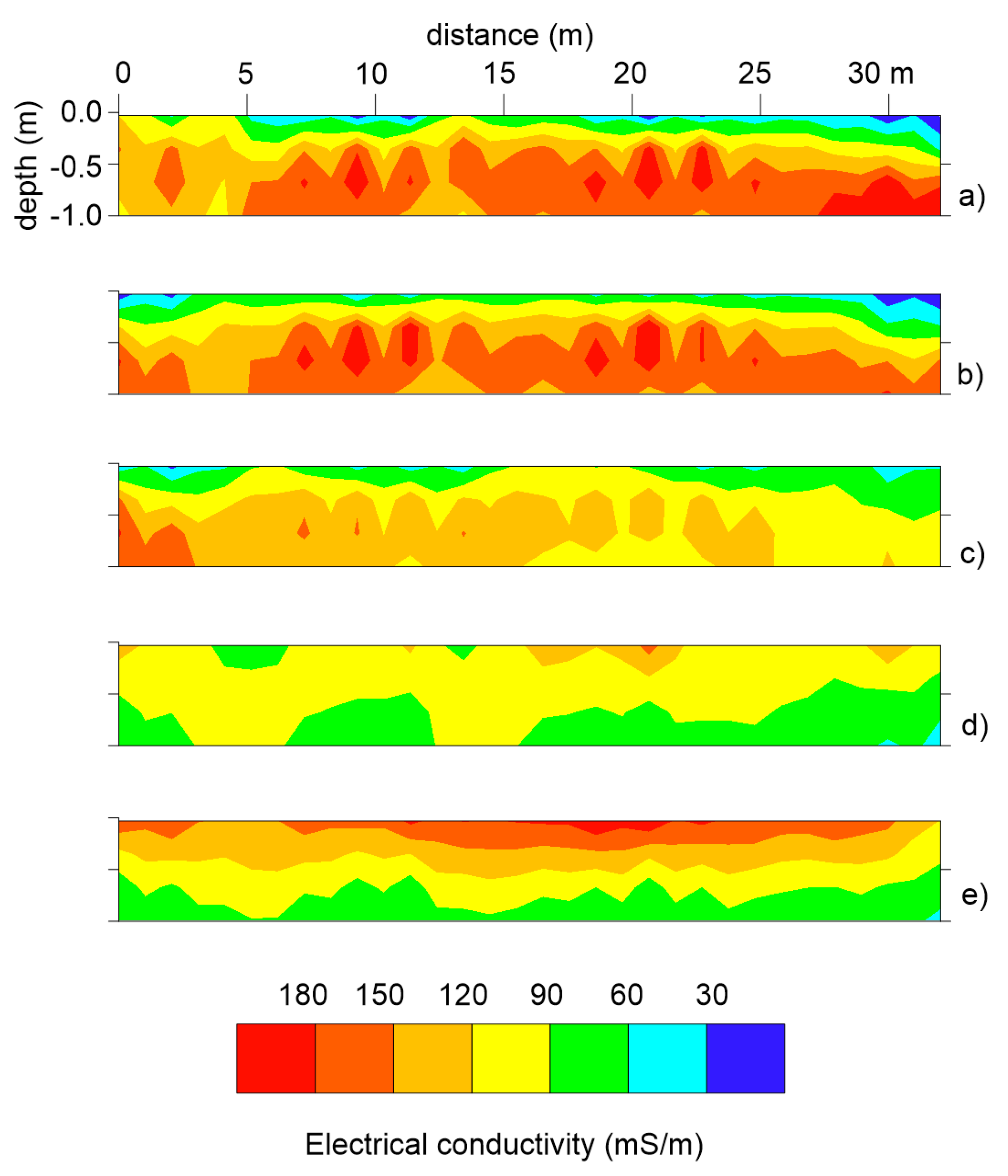
Figure 5.
Normalized EC differences over time for plot A after: a) 14 days; b) 28 days; c) 41 days; d) 66 days.
Figure 5.
Normalized EC differences over time for plot A after: a) 14 days; b) 28 days; c) 41 days; d) 66 days.
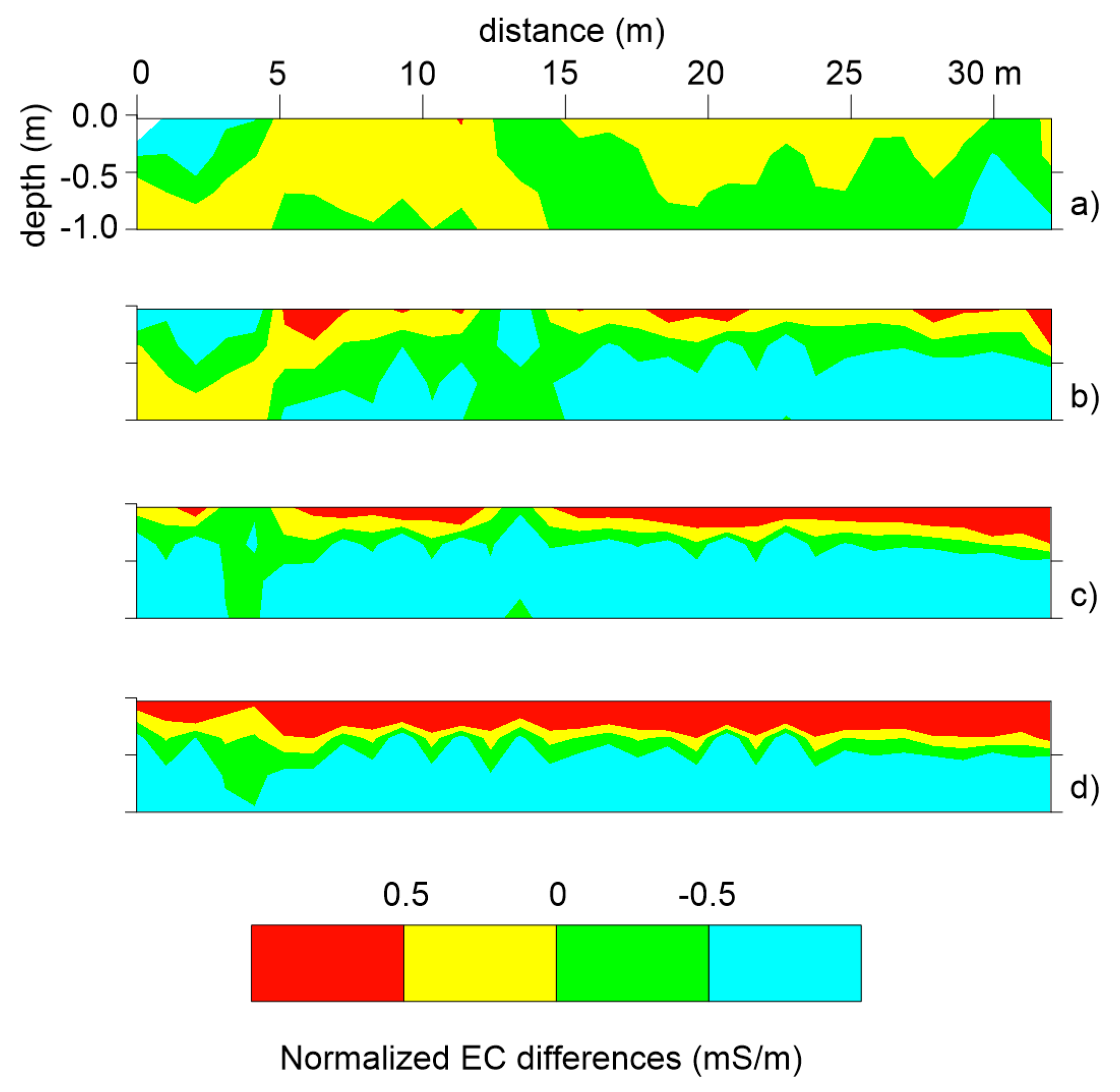
Figure 6.
Observed vs calculated data for each time point observation for plot A: a) 26th June; b) 10th July; c) 24th July; d) 6th August; e) 31st August.
Figure 6.
Observed vs calculated data for each time point observation for plot A: a) 26th June; b) 10th July; c) 24th July; d) 6th August; e) 31st August.
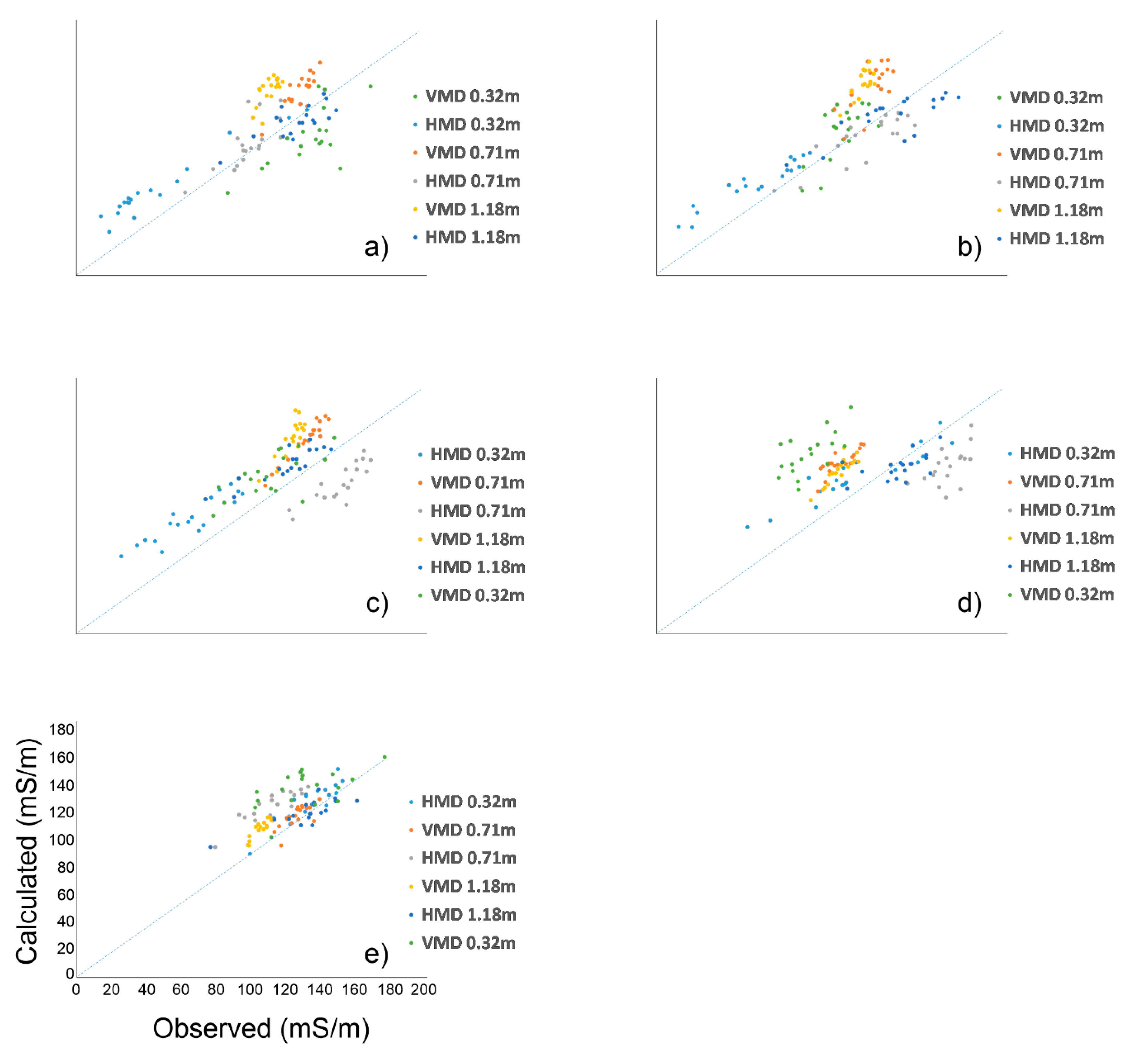
Figure 7.
Inverted EC for transect corresponding to plot B at five different time points: a) 26th June; b) 10th July; c) 24th July; d) 6th August; e) 31st August.
Figure 7.
Inverted EC for transect corresponding to plot B at five different time points: a) 26th June; b) 10th July; c) 24th July; d) 6th August; e) 31st August.
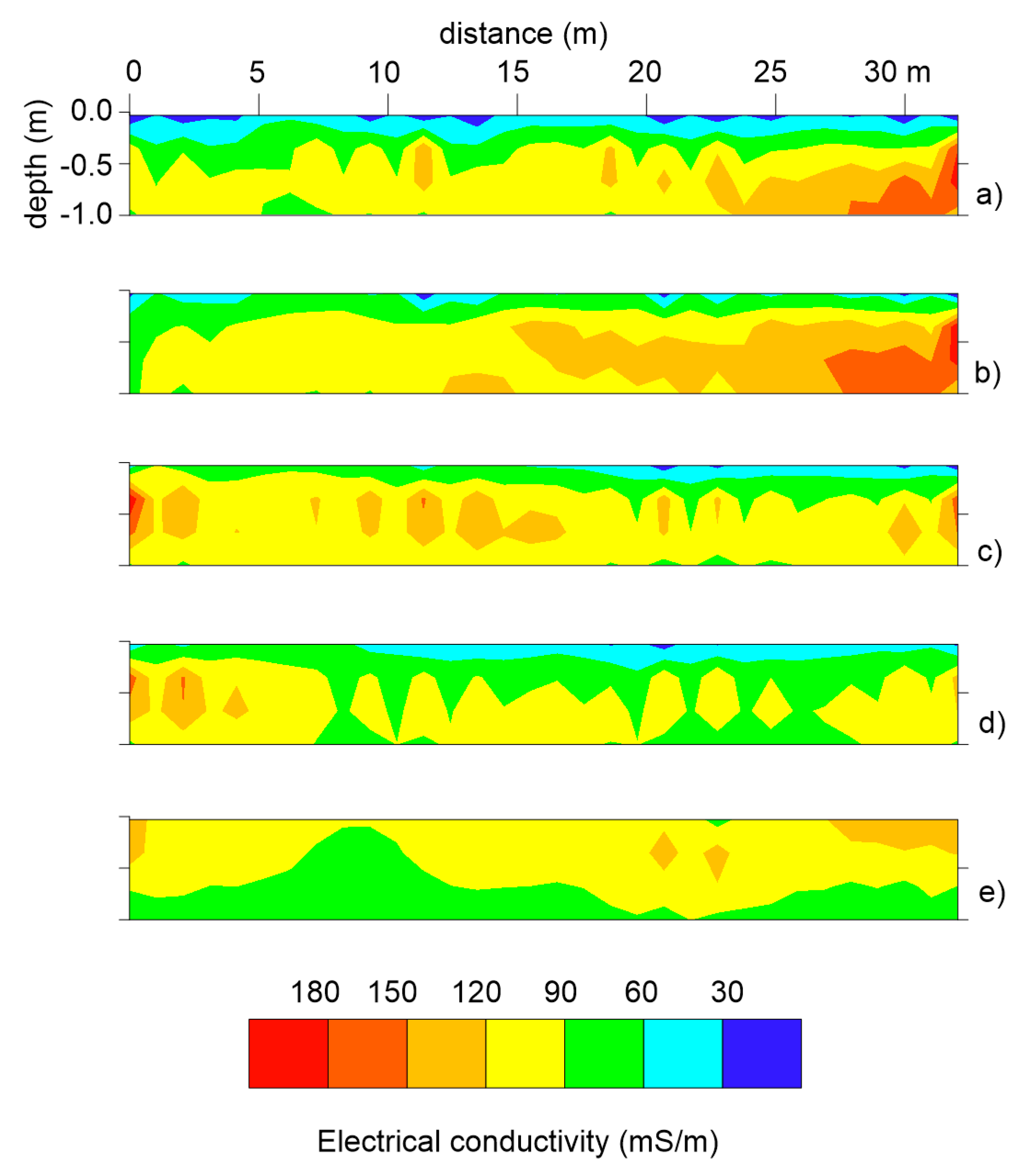
Figure 8.
Normalized EC differences over time for plot B after: a) 14 days; b) 28 days; c) 41 days; d) 66 days.
Figure 8.
Normalized EC differences over time for plot B after: a) 14 days; b) 28 days; c) 41 days; d) 66 days.
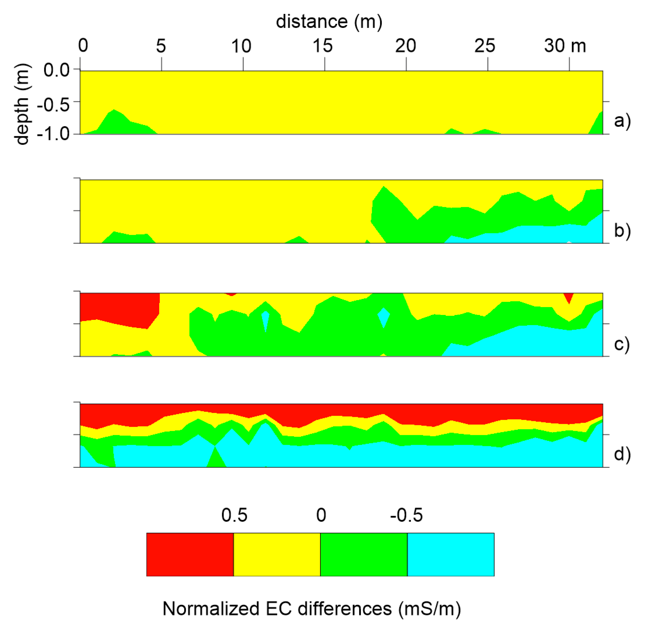
Figure 9.
Inverted EC for transect belonging to plot C at five different time points: a) 26th June; b) 10th July; c) 24th July; d) 6th August; e) 31st August.
Figure 9.
Inverted EC for transect belonging to plot C at five different time points: a) 26th June; b) 10th July; c) 24th July; d) 6th August; e) 31st August.
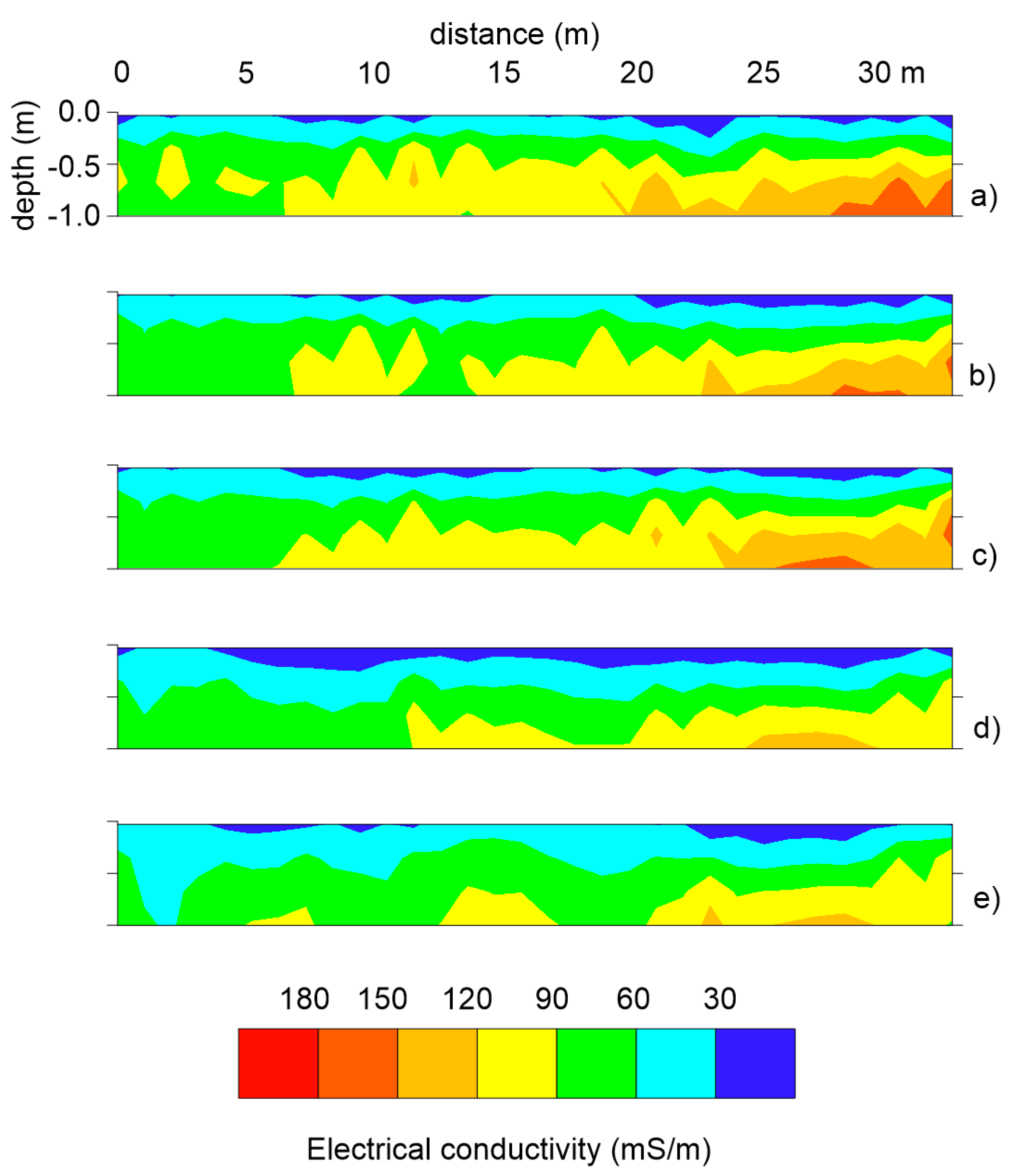
Figure 10.
Normalized EC differences over time for plot C after: a) 14 days; b) 28 days; c) 41 days; d) 66 days.
Figure 10.
Normalized EC differences over time for plot C after: a) 14 days; b) 28 days; c) 41 days; d) 66 days.
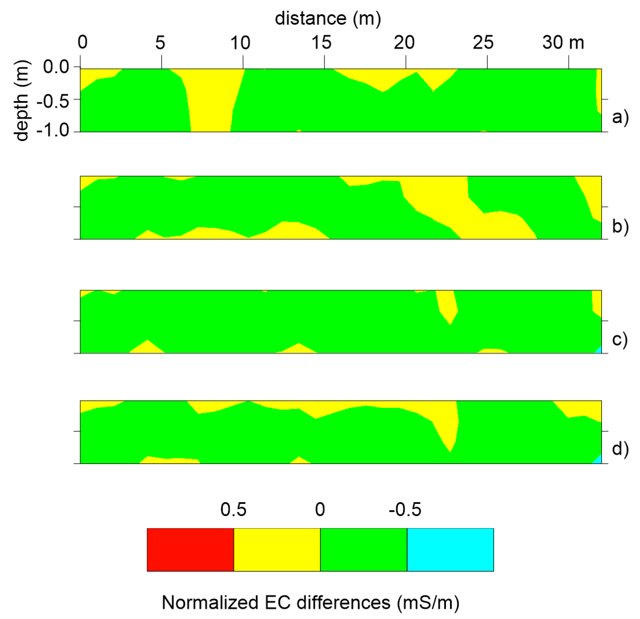
Figure 11.
Changes in EC at the end of the irrigation season for a: plot A; b) plot B; c) plot C. .
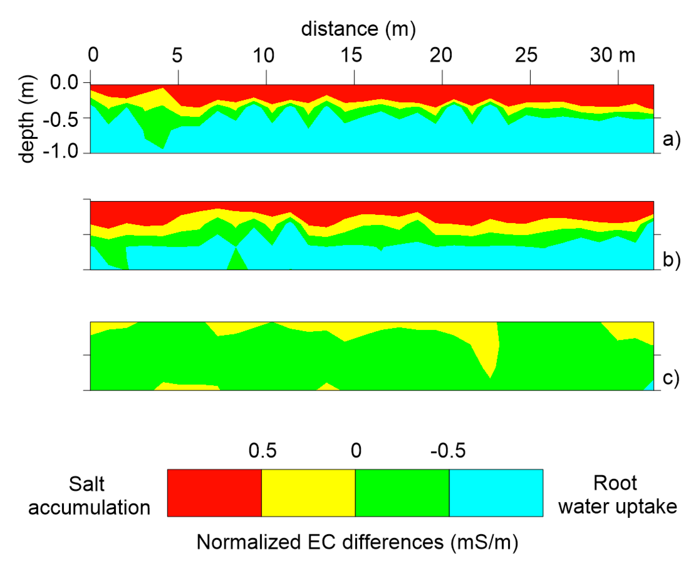
Figure 12.
Inverted EC vs ECe calibration function.
Disclaimer/Publisher’s Note: The statements, opinions and data contained in all publications are solely those of the individual author(s) and contributor(s) and not of MDPI and/or the editor(s). MDPI and/or the editor(s) disclaim responsibility for any injury to people or property resulting from any ideas, methods, instructions or products referred to in the content. |
© 2024 by the authors. Licensee MDPI, Basel, Switzerland. This article is an open access article distributed under the terms and conditions of the Creative Commons Attribution (CC BY) license (http://creativecommons.org/licenses/by/4.0/).
Copyright: This open access article is published under a Creative Commons CC BY 4.0 license, which permit the free download, distribution, and reuse, provided that the author and preprint are cited in any reuse.


